A Primer on Bayesian Neural Networks: Review and Debates

mystyle [0][][]0

a

A Primer on Bayesian Neural Networks:
Review and Debates

Julyan Arbel¹, Konstantinos Pitas¹, Mariia Vladimirova², Vincent Fortuin³

¹Centre Inria de l’Université Grenoble Alpes, France
²Criteo AI Lab, Paris, France
³Helmholtz AI, Munich, Gremany

1 Introduction

Motivation. Technological advancements have sparked an increased interest in the development of models capable of acquiring knowledge and performing tasks that resemble human abilities. These include tasks such as object recognition and scene segmentation in images, speech recognition in audio signals, and natural language understanding. They are commonly referred to as artificial intelligence (AI) tasks. AI systems possess the remarkable ability to mimic human thinking and behavior.

Machine learning, a subset of artificial intelligence, encompasses a fundamental aspect of AI—learning the underlying relationships within data and making decisions without explicit instructions. Machine learning algorithms autonomously learn and enhance their performance by leveraging their output. These algorithms do not rely on explicit instructions to generate desired outcomes; instead, they learn by analyzing accessible datasets and comparing them with examples of the desired output.

Deep learning, a specialized field within machine learning, focuses on algorithms inspired by the structure and functioning of the human brain, known as (artificial) neural networks. Deep learning concepts enable machines to acquire human-like skills. Through deep learning, computer models can be trained to perform classification tasks using inputs such as images, text, or sound. Deep learning has gained popularity due to its ability to achieve state-of-the-art performance. The training of these models involves utilizing large labeled datasets in conjunction with neural network architectures.

Neural networks, or NNs, are particularly effective deep learning models that can solve a wide range of problems. They are now widely employed across various domains. For instance, they can facilitate translation between languages, guide users in banking applications, or even generate artwork in the style of famous artists based on simple photographs. However, neural networks are often regarded as black boxes due to the lack of intuitive interpretations that would allow us to trace the flow of information from input to output.

In certain industries, the acceptance of AI algorithms necessitates explanations. This requirement may stem from regulations encompassed in the concept of AI safety or from human factors. In the field of medical diagnosis and treatment, decisions based on AI algorithms can have life-changing consequences. While AI algorithms excel at detecting various health conditions by identifying minute details imperceptible to the human eye, doctors may hesitate to rely on this technology if they cannot explain the rationale behind its outcomes.

In the realm of finance, AI algorithms can assist in tasks such as assigning credit scores, evaluating insurance claims, and optimizing investment portfolios, among other applications. However, if these algorithms produce biased outputs, it can cause reputational damage and even legal implications. Consequently, there is a pressing need for interpretability, robustness, and uncertainty estimation in AI systems.

The exceptional performance of deep learning models has fueled research efforts aimed at comprehending the mechanisms that drive their effectiveness. Nevertheless, these models remain highly opaque, as they lack the ability to provide human-understandable accounts of their reasoning processes or explanations. Understanding neural networks can significantly contribute to the development of safe and explainable AI algorithms that could be widely deployed to improve people’s lives. The Bayesian perspective is often viewed as a pathway toward trustworthy AI. It employs probabilistic theory and approximation methods to express and quantify uncertainties inherent in the models. However, the practical implementation of Bayesian approaches for uncertainty quantification in deep learning models often incurs significant computational costs and necessitates the use of improved approximation techniques.

Objectives and outline. The recent surge of research interest in Bayesian deep learning has spawned several notable review articles that contribute valuable insights to the field. For instance, Jospin et al., (2022) present a useful contribution by offering practical implementations in Python, enhancing the accessibility of Bayesian deep learning methodologies. Another significant review by Abdar et al., (2021) provides a comprehensive assessment of uncertainty quantification techniques in deep learning, encompassing both frequentist and Bayesian approaches. This thorough examination serves as an essential resource for researchers seeking to grasp the breadth of available methods. While existing literature delves into various aspects of Bayesian neural networks, Goan and Fookes, (2020) specifically focuses on inference algorithms within BNNs. However, the comprehensive coverage of prior modeling, a critical component of BNNs, is not addressed in this review. Conversely, Fortuin, (2022) presents a meticulous examination of priors utilized in diverse Bayesian deep learning models, encompassing BNNs, deep Gaussian processes, and variational auto-encoders (VAEs). This review offers valuable insights into the selection and impact of priors across different Bayesian modeling paradigms.

In contrast to these works, our objective is to offer an accessible and comprehensive guide to Bayesian neural networks, catering to both statisticians and machine learning practitioners. The target audience comprises statisticians with a potential background in Bayesian methods but lacking deep learning expertise, as well as machine learners proficient in deep neural networks but with limited exposure to Bayesian statistics. Assuming no prior familiarity with either deep learning or Bayesian statistics, we provide succinct explanations of both domains in Section 2 and Section 3, respectively. These sections serve as concise reminders, enabling readers to grasp the foundations of each field. Subsequently, in Section 4, we delve into Bayesian neural networks, elucidating their core concepts, with a specific emphasis on frequently employed priors and inference techniques. By addressing these fundamental aspects, we equip the reader with a solid understanding of BNNs and their associated methodologies. Furthermore, in Section 5, we analyze the principal challenges encountered by contemporary Bayesian neural networks. This exploration provides readers with a comprehensive overview of the obstacles inherent to this field, highlighting areas for further investigation and improvement. Ultimately, Section 6 concludes our guide, summarizing the key points and emphasizing the significance of Bayesian neural networks. By offering this cohesive resource, our goal is to empower statisticians and machine learners alike, fostering a deeper understanding of BNNs and facilitating their broader application in practice.

2 Neural networks and statistical learning theory

The inception of neural network models can be traced back to 1955 when the first model, known as the perceptron, was constructed (Rosenblatt,, 1958). Subsequently, significant advancements have taken place in this field, notably the discovery of the backpropagation algorithm in the 1980s (Rumelhart et al.,, 1986). This algorithm revolutionized neural networks by enabling efficient training through gradient-descent-based methods. However, the current era of profound progress in deep learning commenced in 2012 with a notable milestone: convolutional neural networks, when trained on graphics processing units (GPUs) for the first time, achieved exceptional performance on the ImageNet task (Krizhevsky et al.,, 2012). This breakthrough marked a significant turning point and propelled the rapid advancement of deep learning methodologies.

Definition and notations. Neural networks are hierarchical models made of layers: an input, several hidden layers, and an output, see Figure 1. The number of hidden layers $L$ is called depth. Each layer following the input layer consists of units which are linear combinations of previous layer units transformed by a nonlinear function, often referred to as the nonlinearity or activation function denoted by $\phi:\mathbb{R}\to\mathbb{R}$. Given an input $\bm{x}\in\mathbb{R}^{N}$ (for instance an image made of $N$ pixels), the $\ell$-th hidden layer consists of two vectors whose size is called the width of layer, denoted by $H_{\ell}$, where $\ell=1,\dots,L$. The vector of units before application of the non-linearity is called pre-nonlinearity (or pre-activation), and is denoted by $\bm{g}^{(\ell)}=\bm{g}^{(\ell)}(\bm{x})$, while the vector obtained after element-wise application of $\phi$ is called post-nonlinearity (or post-activation) and is denoted by $\bm{h}^{(\ell)}=\bm{h}^{(\ell)}(\bm{x})$. More specifically, these vectors are defined as

$$\bm{g}^{(\ell)}(\bm{x})=\bm{w}^{(\ell)}\bm{h}^{(\ell-1)}(\bm{x}),\quad\bm{h}^{(\ell)}(\bm{x})=\phi(\bm{g}^{(\ell)}(\bm{x})),$$ (1)

where $\bm{w}^{(\ell)}$ is a weight matrix of dimension $H_{\ell}\times H_{\ell-1}$ including a bias vector, with the convention that $H_{0}=N$, the input dimension.

Figure 1: Simple fully-connected neural network architecture.

Supervised learning. We denote the learning sample $(X,Y)=\{(\bm{x}_{i},\bm{y}_{i})\}^{n}_{i=1}\in(\mathcal{X}\times\mathcal{Y})^{n}$, which contains $n$ input-output pairs. Observations $(X,Y)$ are assumed to be randomly sampled from a distribution $\mathfrak{D}$. Thus, we denote $(X,Y)\sim\mathfrak{D}^{n}$ the i.i.d observation of $n$ elements. We define the test set $(X_{\mathrm{test}},Y_{\mathrm{test}})$ of $n_{\mathrm{test}}$ samples in a similar way to that of the learning sample. We consider some loss function $\mathcal{L}:\mathcal{F}\times\mathcal{X}\times\mathcal{Y}\rightarrow\mathbb{R}$, where $\mathcal{F}$ is a set of predictors $f:\mathcal{X}\rightarrow\mathcal{Y}$. We also denote the empirical risk $\mathcal{R}^{\mathcal{L}}_{n}(f)=(1/n)\sum_{i}\mathcal{L}(f(\bm{x}_{i}),\bm{y}_{i})$ and the risk

$$\mathcal{R}^{\mathcal{L}}_{\mathfrak{D}}(f)=\bm{\mathrm{E}}_{(\bm{x},\bm{y})\sim\mathfrak{D}}\,\mathcal{L}(f(\bm{x}),\bm{y}).$$ (2)

The minimizer of $\mathcal{R}^{\mathcal{L}}_{\mathfrak{D}}$ is called Bayes optimal predictor $f^{*}=\operatorname*{arg\,min}_{f:\mathcal{X}\to\mathcal{Y}}\mathcal{R}^{\mathcal{L}}_{\mathfrak{D}}(f)$. The minimal risk $\mathcal{R}^{\mathcal{L}}(f^{*})$, called Bayes risk, is achieved by the Bayes optimal predictor $f^{*}$.

Returning to neural networks, we denote their vectorized weights by $\bm{w}\in\mathbb{R}^{d}$ with $d=\sum_{\ell=1}^{L}H_{\ell-1}H_{\ell}$, such that $f(\bm{x})=f_{\bm{w}}(\bm{x})$. The goal is to find the optimal weights such that the neural network output $\bm{y}_{i}^{*}$ for input $\bm{x}_{i}$ is the closest to the given label $\bm{y}_{i}$, which is estimated by a loss function $\mathcal{L}$. In the regression problem, for example, the loss function $\mathcal{L}$ could be the mean-squared error $\|\bm{y}_{i}^{*}-\bm{y}_{i}\|^{2}$. The optimization problem is then to minimize the empirical risk:

$$\hat{\bm{w}}=\operatorname*{arg\,min}_{\bm{w}}\mathcal{R}^{\mathcal{L}}_{n}(f_{\bm{w}}).$$

With optimal weights $\hat{\bm{w}}$, the empirical risk $\mathcal{R}^{\mathcal{L}}_{n}(\hat{f})$ is small and should be close to the Bayes risk $\mathcal{R}^{\mathcal{L}}(f^{*})$.

Training. The main workhorse of neural network training is gradient-based optimization:

$$\bm{w}\leftarrow\bm{w}-\eta\,\nabla_{\bm{w}}\mathcal{R}^{\mathcal{L}}_{n}(f_{\bm{w}}),$$ (3)

where $\eta>0$ is a step size, or learning rate, and the gradients are computed as products of gradients between each layer from right to left, a procedure called backpropagation (Rumelhart et al.,, 1986), thus making use of the chain rule and efficient implementations for matrix-vector products. For large datasets, this optimization is often replaced by stochastic gradient descent (SGD), where gradients are approximated on some randomly chosen subsets called batches (Robbins and Monro,, 1951). In this case, it requires a careful choice of the learning rate parameter. For a survey on different optimization methods, see, for example, Sun et al., 2019a . For the optimization procedure, another important aspect is how to choose the weight initialization; we discuss this in detail in Section 5.1.1.

2.1 Choice of architecture

With the progress in deep learning, different neural network architectures have been introduced to better adapt to different learning problems. Knowledge about the data allows encoding specific properties into the architecture. Depending on the architecture, this results (among other benefits) in better feature extraction, a reduced number of parameters, invariance or equivariance to certain transformations, robustness to distribution shifts and more numerically stable optimization procedures. We shortly review some important models and refer the reader to Sarker, (2021) for a more in-depth overview of recent techniques.

Convolutional neural networks (CNNs) are widely used in computer vision. Image data has spatial features that refer to the arrangement of pixels and their relationship. For example, we can easily identify a human’s face by looking at specific features like eyes, nose, mouth, etc. CNNs were introduced to capture spatial features by using convolutional layers, a particular case of the fully-connected layers described above, where certain sets of parameters are shared (LeCun et al.,, 1989; Krizhevsky et al.,, 2012). Convolutional layers perform a dot product of a convolution kernel with the layer’s input matrix. As the convolution kernel slides along the input matrix for the layer, the convolution operation generates a feature map of smaller dimension which serves as an input to the next layer. It introduces the concept of parameter sharing where the same kernel, or filter, is applied across different input parts to extract the relevant features from the input.

Recurrent neural networks (RNNs) are designed to save the output of a layer by adding it back to the input (Rumelhart et al.,, 1986; Hochreiter and Schmidhuber,, 1997). During training, the recurrent layer has some information from the previous time-step. Such neural networks are advantageous for sequential data where each sample can be assumed to be dependent on preceding ones.

Residual neural networks (ResNets) have residual blocks which add the output from the previous layer to the output of the current layer, a so-called skip-connection (He et al., 2016a, ). It allows training very deep neural networks by ensuring that deeper layers in the model will perform at least as well as layers preceding them. (He et al., 2016b, ).

Transformers are a type of neural network architecture that is almost entirely based on the attention mechanism (Vaswani et al.,, 2017). The idea behind attention is to find and focus on small, but important, parts of the input data. Transformers show better results than convolutional or residual networks on some tasks with big datasets such as image classification with JFT-300M (300M images), or English-French machine translation with WMT-2014 (36M sentences, split into a 32000 token vocabulary).

An open question in deep learning is why deep neural networks (NNs) achieve state-of-the-art performance in a significant number of applications. The common belief is that neural networks’ complexity and over-parametrization result in tremendous expressive power, beneficial inductive bias, flexibility to avoid overfitting and, therefore, the ability to generalize well. Yet, the high dimensionalities of the data and parameter spaces of these models make them challenging to understand theoretically. In the following, we review these open topics of research as well as the current scientific consensus on them.

2.2 Expressiveness

The expressive power describes neural networks’ ability to approximate functions. In the late 1980s, a line of works established a universal approximation theorem, stating that one-hidden-layer neural networks with a suitable activation function could approximate any continuous function on a compact domain, that is $f:[0,1]^{N}\to\mathbb{R}$, to any desired accuracy (Cybenko,, 1989; Funahashi,, 1989; Hornik et al.,, 1989; Barron,, 1994). The obstacle is that the size of such networks may be exponential in the input dimension $N$, which makes them highly prone to overfitting as well as impractical, since adding extra layers in the model is often a cheaper way to increase the representational power of the neural network. More recently, Telgarsky, (2016) studied which functions neural networks could represent by focusing on the choice of the architecture and showed that deeper models are more expressive. Chatziafratis et al., 2020b ; Chatziafratis et al., 2020a extended this result by obtaining width-depth trade-offs.

Another approach is to analyze the finite-sample expressiveness of neural networks. Zhang et al., 2017a state that as soon as the number of parameters of a network is greater than the input sample size, even a simple two-layer neural network can represent any function of the input sample. Though neural networks are theoretically expressive, the core of the learning problem lies in their complexity, and research focuses on obtaining complexity bounds.

In general, the ability to approximate or to express specific functions can be considered as explicit inductive bias which we discuss in detail in the next section.

2.3 Inductive bias

By choosing a design and a training procedure for a model assigned to a given problem, we make some assumptions on the problem structure. These assumptions are summed in the term inductive bias, i.e., prior preferences for specific models and problems.

Examples. For instance, the linear regression model is built on the assumption of a linear relationship between the target variable and the features. The knowledge that the data is of a linear nature is embedded into the model. Because of this limitation of the linearity of the model, linear regression is bound to perform poorly for data in where the target variable does not linearly depend on features, see the left plot of Figure 2. This assumption of a linear relationship between the target and the features is the inductive bias of linear regression. In the $k$-nearest neighbours model, the inductive bias is that the answer for any object should be calculated only on the basis of what values of the answers were in the elements of the training sample closest to this object, see the right plot of Figure 2. In the non-linear regression, the assumption is some non-linear function.

linear regression                                 $k$-nearest neighbours

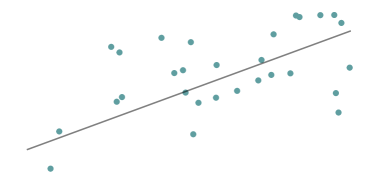
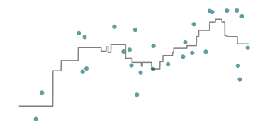
Figure 2: Example of using the linear regression (left) and $k$-nearest neighbours regression (right) models on simulated data points.

Importance. The goal of a machine learning model is to derive a general rule for all elements of a domain based on a limited number of observations. In other words, we want the model to generalize to data it has not seen before. Such generalization is impossible without the presence of inductive bias in the model because the training sample is always finite. From a finite set of observations, without making any additional assumptions about the data, a general rule can be deduced in an infinite number of ways. Inductive bias is additional information about the nature of the data for the model; a way to show models which way to think. It allows the model to prioritize one generalization method over another. Thus, when choosing a model for training to solve a specific problem, one needs to choose a model whose inductive bias better matches the nature of the data and better allows to solve this problem. The introduction of any inductive bias into a machine learning model relies on certain characteristics of the model architecture, training algorithm and manipulations on training data.

Inductive bias and training data. One can also consider inductive bias through training data. The fewer data, the more likely the model chooses a poor generalization method. If the training sample is small, models such as neural networks are often overfitted. For example, when solving the problem of classifying images of cats and dogs, sometimes attention is paid to the background and not to the animals themselves. But people, unlike neural networks, can quickly learn on the problem of classifying cats and dogs, having only a dozen pictures in the training set. This is because people have additional inductive bias: we know that there is a background in the picture, and there is an object, and during the classification of pictures, you need to pay attention only to the object itself. And the neural network before training does not know about any “backgrounds” and “objects”—it is simply given different pictures and asked to learn how to distinguish them. Thus, the smaller the training sample and the more complex the problem, the stronger inductive bias is required to be invested in the model device for successful model training.

Conversely, the more extensive and more diverse the training set, the more knowledge about the nature of the data the model receives during training. This means that the less likely the model is to choose a “bad” generalization method that will work poorly on data outside the training set. Thus, the more data you have, the better the model will train.

One of the tricks to increase the dataset is to artificially augment the training set by introducing distortions into the inputs, a procedure known as data augmentation. Suppose we are trying to classify images of objects or handwritten digits. Each time we visit a training example, we can randomly distort it, for instance, by shifting it by a few pixels, adding noise, rotating it slightly, or applying some sort of warping. This can increase the effective size of the training set and make it more likely that any given test example has a closely related training example. The data augmentation procedure is a sort of inductive bias because it requires the knowledge of how to construct additional data points, such as if the object or part of the object can be rotated, zoomed in, etc.

Inductive bias and simplicity. The no free lunch theorem states that no single learning algorithm can succeed on all possible problems (Wolpert,, 1996). It is, thus, essential to enforce a form of simplicity in the algorithm, typically by restricting the class of models to be learned, which may reflect prior knowledge about the problem being tackled. This is associated with inductive bias which should encode the prior knowledge to seek for efficiency. In the context of neural networks, one form of simplicity is in the choice of architecture, such as using convolutional neural networks (LeCun et al.,, 1989) when learning from image data. Another example is sparsity, which may seek models that only rely on a few relevant variables out of many available ones and can be achieved through some regularization methods (Tibshirani,, 1996).

Inductive bias of neural network architecture. A number of deep neural network architectures have been designed with the aim of improving the inductive bias of the corresponding predictor. Here we review two popular neural network architectures that encode useful inductive biases.

Convolutional neural networks (CNNs). The inductive bias of convolutional layers (LeCun et al.,, 1989) is the assumption of compactness and translation invariance. The convolution filter is designed in such a way that at one time it captures a compact part of the entire image (for example, a $3\times 3$ pixels square), regardless of the distant pixels of the image. Also in the convolutional layer, the same filter is used to process the entire image (the same filter processes all $3\times 3$ pixels square). It turns out that the convolutional layer is designed in such a way that its inductive bias correlates well with the nature of images and objects on them, which is why convolutional neural networks are so efficient at processing images (Krizhevsky et al.,, 2012). This is an example of the desired, or explicit inductive bias. What makes data efficiently learnable by fitting a huge neural network with a specific algorithm? Is there implicit inductive bias? Ulyanov et al., (2018) demonstrate that the output of a convolutional neural network with randomly initialized weights corresponds to a deep image prior, i.e. non-trivial image properties, before training. It means that how convolutional neural networks are designed, their architecture itself, helps to encode the information from images. Geirhos et al., (2019) show that convolutional neural networks have implicit inductive bias concerning the texture of images: it turns out that convolutional networks are designed in such a way that when processing images, they pay more attention to textures rather than to the shapes of objects. To get rid of this undesirable behavior, the images from the training dataset are augmented so that the dataset contains more images of the same shape, but with different types of textures (Li et al.,, 2021). Despite the popularity of the topic, the implicit inductive bias in neural networks is still an open question due to the complexity of the models.

Visual transformers (Dosovitskiy et al.,, 2021) are a type of neural network architecture that shows better results than convolutional networks on some tasks, including, for example, classification of images from the JFT-300M dataset. This dataset consists of 300 million images, while Imagenet has 1.2 million images. The visual transformer is almost entirely based on the attention mechanism (Vaswani et al.,, 2017), so the model has the inductive bias that attention has which consists in a shift towards simpler functions. But like convolutions, transformers also have the implicit inductive bias of neural networks (Morrison et al.,, 2021). Though there is still a lot of ongoing research on transformers, the inductive bias of transformers is much simpler than that of convolutional neural networks, as the former models impose fewer restrictions than the latter models. Here we see confirmation that the larger dataset we have at our disposal, the less inductive bias is required, and the better the model can learn for the task. Therefore, transformers have simple inductive bias and show state-of-the-art results in image processing, but they require a lot of data. On the contrary, convolutional neural networks have a strong inductive bias, and they perform well on smaller datasets. Recently, d’Ascoli et al., (2021) combined the transformer and convolutional neural network architectures, introducing the CONVIT model. This model is able to process images almost as well as transformers, while requiring less training data.

2.4 Generalization and overfitting

When we train a machine learning model, we do not just want it to learn to model the training data. We want it to generalize to data it has not seen before. Fortunately, there is a way to measure an algorithm’s generalization performance: we measure its performance on a held-out test set, consisting of examples it has not seen before. If an algorithm works well on the training set but fails to generalize, we say it suffers from overfitting. Modern machine learning systems based on deep neural networks are usually over-parameterized, i.e., the number of parameters in the model is much larger than the size of the training data, which makes these systems prone to overfitting.

Classical regime. Let us randomly divide the original dataset into a train, validation and test set. The model is trained by optimizing the training error computed on the train set, then its performance is checked by computing the validation error on the validation set. After tuning any existing hyperparameters by checking the validation error, the model (or models) are then evaluated on final time on the test set.

During the training procedure, the model can suffer from overfitting and underfitting (see Figure 3 for an illustration), which can be described in terms of training and testing errors.

Overfitting is a negative phenomenon that occurs when a learning algorithm generates predictions that fit too closely or exactly to a particular dataset and are therefore not suitable for applying the algorithm to additional data or future observations. In this case, the training error is low but the error computed on a test set is high. The model finds dependencies in the train set which does not hold in the test set. As a result, the model has high variance, a problem caused by being highly sensitive to small deviations in the training set.

The opposite of overfitting is underfitting, in which the learning algorithm does not provide a sufficiently small average error on the training set. Underfitting occurs when insufficiently complex models are used or the training is stopped too early. In this case, the error is high for both train and test sets. As a result, the model has high bias, an error of incorrect assumptions in the learning algorithm.

The goal is to find the best strategy to reduce overfitting and improve the generalization, or, in other words, reduce the trained model’s bias and variance. Ensembles can be used to eliminate high variance and high bias. For example, the boosting procedure of several models with high bias can get a model with a reduced bias. In another case, when bagging, several low-bias models are connected, and the resulting model can reduce the variance. But in general, reducing one of the adverse effects leads to an increase in the other. This conflict in an attempt to simultaneously minimize bias and variance is called the bias-variance trade-off. This trade-off is achieved in the minimum of the test error, see the classical regime region on Figure 3.

Figure 3: Examples of underfitting, optimum solution, and overfitting in a toy classification problem. The green dots and violet squares represent two classes. The lines represent different models that classify the data. The left plot shows the result of using a model that is too simple or underfitted for the presented dataset, while the right plot shows an overfitted model.

Modern regime. In the past few years, it was shown that when increasing the model size beyond the number of training examples, the model’s test error can start decreasing again after reaching the interpolation peak, see Figure 4. This phenomenon is called double-descent by Belkin et al., (2019) who demonstrated it for several machine learning models, including a two-layer neural network. Nakkiran et al., (2021) extensively study this double-descent phenomenon for deep neural network models and show the double-descent phenomenon occurs when varying the width of the model or the number of iterations during the optimization. Moreover, the double-descent phenomenon can be observed as a function of dataset size, where more data sometimes lead to worse test performance. It is not fully understood yet why this phenomenon occurs in machine learning models and which inductive biases are responsible for it. However, it is important to take this aspect into account while choosing strategies to improve generalization.

Figure 4: Illustration of the double-descent phenomenon.

Strategies. One reason for overfitting is the lack of training data, making the learned distribution not mirror the real underlying distribution. Collecting data arising from all possible parts of the domain to train machine learning models is prohibitively expensive and even impossible. Therefore, enhancing the generalization ability of models is vital in both industry and academic fields. Data augmentation methods, which are discussed above in the context of inductive bias, extract more information from the original dataset through augmentations, thus, help to improve the generalization.

Many strategies for increasing generalization performance focus on the model’s architecture itself. Regularization methods are used to encourage a lower complexity of a model. Functional solutions such as dropout regularization (Srivastava et al.,, 2014), batch normalization (Ioffe and Szegedy,, 2015), transfer learning (Weiss et al.,, 2016), and pretraining (Erhan et al.,, 2010) have been developed to try to adapt deep learning to applications on smaller datasets. Another approach is to treat the number of training epochs as a hyperparameter and to stop training if the performance of the model on the test dataset starts to degrade, e.g., loss begins to increase or accuracy begins to decrease. This procedure is called early stopping.

Though explicit regularization techniques are known to improve generalization, their absence does not imply poor generalization performance for deep learning models. Indeed, Zhang et al., 2017a argue that neural networks have implicit regularizations; for instance, stochastic gradient descent tends to converge to small norm solutions. The early stopping procedure can also be viewed as implicit regularization method as it implicitly forces to use a smaller network with less capacity (Zhang et al., 2017a, ; Zhang et al.,, 2021).

Generalization bounds. We are often interested in making the discussion on training, validation, and testing sets formal, so as to ensure that our neural network will work well on new data with high probability. We are thus often interested in finding a bound on risk $\mathcal{R}^{\mathcal{L}}_{\mathfrak{D}}(f)=\bm{\mathrm{E}}_{(\bm{x},\bm{y})\sim\mathfrak{D}}\,\mathcal{L}(f(\bm{x}),\bm{y})$ with high probability.

The most common way of bounding the above in the context of deep neural networks is by use of a test set (Langford,, 2005; Kääriäinen and Langford,, 2005). One first trains a predictor $f$ using a training set $\mathcal{D}_{\mathrm{train}}$, and then computes a test risk $\mathcal{R}^{\mathcal{L}}_{\mathcal{D}_{\mathrm{test}}}(f)$. For $n_{\mathrm{test}}$ test samples, and in the classification setting, this can be readily turned into a bound on the risk $\mathcal{R}^{\mathcal{L}}_{\mathfrak{D}}(f)$, using a tail bound on the corresponding binomial distribution (Langford,, 2005). However, this approach has some shortcomings. For one it requires a significant number of samples $n_{\text{test}}$. This can be a problem in that these samples cannot be used for training, possibly hindering the performance of the deep network. At the same time, for a number of fields such as healthcare, the cost of obtaining test samples can be prohibitively high (Davenport and Kalakota,, 2019). Finally, even though we can prove that the true risk will be low, we do not get any information about the reason why the classifier performs well in the first place.

As such, researchers often use the empirical risk (on the training set) together with the complexity (Mohri et al.,, 2018) of the classifier to derive bounds roughly of the form

$$\mathcal{R}^{\mathcal{L}}_{\mathfrak{D}}(f)\leq\mathcal{R}^{\mathcal{L}}_{\mathcal{D}_{\mathrm{train}}}(f)+\mathrm{complexity}.$$

Intuitively, the more complex the classifier, the more it is prone to simply memorize the training data, and to learn any discriminative patterns. This leads to high true risk. Traditional data-independent complexity measures such as Rademacher complexity (Mohri et al.,, 2018) and VC-dimension (Blumer et al.,, 1989) are loose for deep neural networks. This is because they intuitively make a single complexity estimate for the neural network for all possible input datasets. Thus they are pessimistic, as a neural network could memorize one dataset (which is difficult) but learn patterns that generalize on another dataset (which might be easy).

Based on the above results, researchers focused on complexity measures which are data-dependent (Golowich et al.,, 2017; Arora et al.,, 2018; Neyshabur et al.,, 2017; Sokolić et al.,, 2016; Bartlett et al.,, 2017; Dziugaite and Roy,, 2017). This means that they assess the complexity of a deep neural network based on the specific instantiation of the weights that we inferred for a given dataset. The tightest data-dependent generalization bounds are currently PAC-Bayes generalization bounds (McAllester,, 1999; Germain et al.,, 2016; Dziugaite and Roy,, 2017; Dziugaite et al.,, 2021). Contrary to the VC-dimension or the Rademacher complexity, these bounds work for stochastic neural networks (which are also the topic of this review). They can be roughly seen as bounding the mutual information between the training set and the deep neural network weights. The main complexity quantity of interest is typically the Kullback–Leibler (KL) divergence between a prior and a posterior distribution over the deep neural network weights (Dziugaite and Roy,, 2017; McAllester,, 1999).

2.5 Limitations of the frequentist approach to deep learning

Although deep learning models have been largely used in many research areas, such as image analysis  (Krizhevsky et al.,, 2012), signal processing (Graves et al.,, 2013), or reinforcement learning (Silver et al.,, 2016), their safety-critical real-world applications remain limited. Here we identify a number of limitations of the frequentist approach to deep learning:

• miscalibrated and/or overconfident uncertainty estimates (Minderer et al.,, 2021);

• non-robustness to out-of-distribution samples (Lee et al., 2018b, ; Mitros and Mac Namee,, 2019; Hein et al.,, 2019; Ashukha et al.,, 2020), and sensitivity to domain shifts (Ovadia et al.,, 2019);

• sensitivity to adversarial attacks by malicious actors (Moosavi-Dezfooli et al.,, 2016, 2017; Wilson et al.,, 2016);

• poor interpretability of a deep neural networks’ inference model (Sundararajan et al.,, 2017; Selvaraju et al.,, 2017; Lim et al.,, 2021; Koh and Liang,, 2017);

• poor understanding of generalization, over-reliance on validation sets (McAllester,, 1999; Dziugaite and Roy,, 2017).

Uncertainty estimates. We typically distinguish between two types of uncertainty (Der Kiureghian and Ditlevsen,, 2009). Data (aleatoric) uncertainty captures noise inherent in the observations. This could be for example sensor noise or motion noise, resulting in uncertainty that cannot be reduced even if more data were to be collected. Model (epistemic) uncertainty derives from the uncertainty on the model parameters, i.e., the weights in case of a neural network (Blundell et al.,, 2015). This uncertainty captures our ignorance about which model generated our collected data. While aleatoric uncertainty remains even for an infinite number of samples, model uncertainty can be explained away given enough data. For an overview on methods for estimating the uncertainty in deep neural networks see Gal, (2016); Gawlikowski et al., (2021).

While NNs often achieve high train and test accuracy, the uncertainty of their predictions is miscalibrated (Guo et al.,, 2017). In particular, in the classification setting, interpreting softmax outputs as per-class probabilities is not well-founded from a statistical perspective. The Bayesian paradigm, by contrast, provides well-founded and well-calibrated uncertainty estimates (Kristiadi et al.,, 2020), by dealing with stochastic predictors and applying Bayes’ rule consistently.

Distribution shift. Traditional machine learning methods are generally built on the iid assumption that training and testing data are independent and identically distributed. However, the iid assumption can hardly be satisfied in real scenarios, resulting in uncertainty problems with in-domain, out-of-domain samples, and domain shifts. In-domain uncertainty is measured on data taken from the training data distribution, i.e. data from the same domain. Out-of-domain uncertainty of the model is measured on data that does not follow the same distribution as the training dataset. Out-of-domain data can include data naturally corrupted with noise or relevant transformations, as well as data corrupted adversarially. Under corruption, the test domain and the training domain differ significantly. However, the model should still not be overconfident in its predictions.

Hein et al., (2019) demonstrate that rectified linear unit (ReLU) networks are always overconfident on out-of-distribution examples: scaling a training point $\bm{x}\in\mathbb{R}^{N}$ with a scalar $a$ yields predictions of arbitrarily high confidence in the limit $a\to\infty$. Modas et al., (2021); Fawzi et al., (2016) discuss that neural networks in the case of classification can suffer from reduced accuracy in the presence of common corruptions. A common remedy is training on appropriately designed data transformations (Modas et al.,, 2021). However, the Bayesian paradigm should again be beneficial. It is expected that the resulting Bayesian neural networks will give more uncertainty in regions far from the training data, thus degrading as images become gradually more corrupted, and diverging from the training data.

Adversarial robustness. As previously mentioned, modern image classifiers achieve high accuracy on iid test sets but are not robust to small, adversarially-chosen perturbations of their inputs. Given an image $\bm{x}$ correctly classified by a neural network, an adversary can usually engineer an adversarial perturbation $\bm{\delta}$ so small that $\bm{x}+\bm{\delta}$ looks just like $\bm{x}$ to the human eye, yet the network classifies $\bm{x}+\bm{\delta}$ as a different, incorrect class. Bayesian neural networks with distributions placed over their weights and biases enable principled quantification of their predictions’ uncertainty. Intuitively, the latter can be used to provide a natural protection against adversarial examples, making BNNs particularly appealing for safety-critical scenarios, in which the safety of the system must be provably guaranteed.

Interpretability. Deep neural networks are highly opaque because they cannot produce human-understandable accounts of their reasoning processes or explanations. There is a clear need for deep learning models that offer explanations that users can understand and act upon (Lipton,, 2018). Some models are designed explicitly with interpretability in mind (Montavon et al.,, 2018; Selvaraju et al.,, 2017). At the same time, a number of techniques have been developed to interpret neural network predictions, including among others gradient-based methods (Sundararajan et al.,, 2017; Selvaraju et al.,, 2017) which create “heatmaps” of the most important features, as well as influence-function-based approaches (Koh and Liang,, 2017). The Bayesian paradigm allows for an elegant treatment of interpretability. Defining a prior is central to the Bayesian paradigm, and selecting it helps analyze which tasks are similar to the current task, how to model the task noise, etc. (see Fortuin et al.,, 2021; Fortuin,, 2022). Furthermore, the Bayesian paradigm incorporates a function-space view of predictors (Khan et al.,, 2019). Compared to the weight-space view, this can result in more interpretable architectures.

Generalization bounds. It is well known that traditional approaches to proving generalization using generalization bounds fail for deterministic deep neural networks. Such generalization bounds are very useful for cases where we have little training data. In such cases, we might not be able to both train the predictor sufficiently and keep a large enough additional set for validation and testing. Therefore, a generalization bound could ensure that we both train on the full data available while at the same time proving generalization. For example, Zhang et al., 2017b ; Golowich et al., (2017) generalization bounds based on Rademacher complexity and the VC dimension provide vacuous bounds on the true error rate (they provide upper bounds larger than 100%). On the contrary, the Bayesian paradigm currently results in the tightest generalization bounds for deep neural networks, in conjunction with a frequentist approach termed PAC-Bayes (Dziugaite and Roy,, 2017). Thus following the Bayesian paradigm is a promising direction for tasks with difficult-to-obtain data.

We introduce the Bayesian paradigm in Section 3 and then review its application to neural networks in Section 4.

3 Bayesian machine learning

Achieving a simultaneous design of adaptive and robust systems presents a significant challenge. In their work, Khan and Rue, (2021) propose that effective algorithms that strike a balance between robustness and adaptivity often exhibit a Bayesian nature, as they can be viewed as approximations of Bayesian inference. The Bayesian approach has long been recognized as a well-established paradigm for working with probabilistic models and addressing uncertainty, particularly in the field of machine learning (Ghahramani,, 2015). In this section, we will outline the key aspects of the Bayesian paradigm, aiming to provide the necessary technical foundation for the application of Bayesian neural networks.

3.1 Bayesian paradigm

The fundamental idea behind the Bayesian approach is to quantify the uncertainty in the inference by using probability distributions. Considering parameters as random variables is in contrast to non-Bayesian approaches, also referred to as frequentist or classic, where parameters are assumed to be deterministic quantities. A Bayesian acts by updating their beliefs as data are gathered according to Bayes’ rule, an inductive learning process called Bayesian inference. The choice of resorting to Bayes’ rule instead of any other has mathematical justifications dating back to works by Cox and by Savage (Cox,, 1961; Savage,, 1972).

Recall the following notations: let a dataset $\mathcal{D}=\{(\bm{x}_{1},\bm{y}_{1}),\dots,(\bm{x}_{n},\bm{y}_{n})\}$, modeled with a data generating process characterized by a sampling model or likelihood $p(\mathcal{D}|\bm{w})$. Let parameters $\bm{w}$ belong to some parameter space denoted by $\bm{\mathcal{W}}$, usually a subset of the Euclidean space $\mathbb{R}^{d}$. A prior distribution $p(\bm{w})$ represents our prior beliefs about the distribution of the parameters $\bm{w}$ (more details in Section 3.2). Note that simultaneously specifying a prior $p(\bm{w})$ and a sampling model $p(\mathcal{D}|\bm{w})$ amounts to describing the joint distribution between parameters $\bm{w}$ and data $\mathcal{D}$, in the form of the product rule of probability $p(\bm{w},\mathcal{D})=p(\bm{w})p(\mathcal{D}|\bm{w})$. The prior and the model are combined with Bayes’ rule to yield the posterior distribution $p(\bm{w}|\mathcal{D})$ as follows:

$$p(\bm{w}|\mathcal{D})=\frac{p(\bm{w})p(\mathcal{D}|\bm{w})}{p(\mathcal{D})}.$$ (4)

The normalizing constant $p(\mathcal{D})$ in Bayes’ rule is called the model evidence or marginal likelihood. This normalizing constant is irrelevant to the posterior since it does not depend on the parameter $\bm{w}$, which is why Bayes’ rule is often written in the form

$$\text{posterior}\propto\text{prior}\times\text{likelihood}.$$

Nevertheless, the model evidence remains critical in model comparison and model selection, notably through Bayes factors. See for example Chapter 28 in MacKay, (2003), and Lotfi et al., (2022) for a detailed exposition in Bayesian deep learning. It can be computed by integrating over all possible values of $\bm{w}$:

$$p(\mathcal{D})=\int p(\mathcal{D}|\bm{w})p(\bm{w})\mathrm{d}\bm{w}.$$ (5)

Using a Bayesian approach, all information conveyed by the data is encoded in the posterior distribution. Often statisticians are asked to communicate scalar summaries in the form of point estimates of the parameters or quantities of interest. A convenient way to proceed for Bayesians is to compute the posterior mean of some quantity of interest $f(\bm{w})$ of the parameters. The problem therefore comes down to numerical computation of the integral

$$\mathbb{E}[f(\bm{w})|\mathcal{D}]=\int f(\bm{w})p(\bm{w}|\mathcal{D})\mathrm{d}\bm{w}.$$ (6)

This includes the posterior mean if $f(\bm{w})=\bm{w}$, as well as predictive distributions. More specifically, let $\bm{y}^{*}$ be a new observation associated to some input $\bm{x}^{*}$ in a regression or classification task; then the prior and posterior predictive distributions are respectively

$$p(\bm{y}^{*}|\bm{x}^{*}) =\mathbb{E}[p(\bm{y}^{*}|\bm{x}^{*},\bm{w})]$$

$$=\int p(\bm{y}^{*}|\bm{x}^{*},\bm{w})p(\bm{w})\mathrm{d}\bm{w},$$

$$\text{and}\quad p(\bm{y}^{*}|\bm{x}^{*},\mathcal{D}) =\mathbb{E}[p(\bm{y}^{*}|\bm{x}^{*},\bm{w})|\mathcal{D}]$$

$$=\int p(\bm{y}^{*}|\bm{x}^{*},\bm{w})p(\bm{w}|\mathcal{D})\mathrm{d}\bm{w}.$$

The posterior predictive distribution is typically used in order to assess model fit to the data, by performing posterior predictive checks. More generally, it allows us to account for model uncertainty, or epistemic uncertainty, in a principled way, by averaging the sampling distribution $p(\bm{y}^{*}|\bm{x}^{*},\bm{w})$ over the posterior distribution $p(\bm{w}|\mathcal{D})$. This model uncertainty is in contrast to the uncertainty associated with data measurement, also called aleatoric uncertainty (see Section 2.5).

3.2 Priors

Bayes’ rule (4) tells us how to update our beliefs, but it does not provide any hint about what those beliefs should be. Often the choice of a prior may be dictated by computational convenience. Let us mention the case of conjugacy: a prior is said to be conjugate to a sampling model if the posterior remains in the same parametric family. Classic examples of such conjugate pairs of [prior, model] include the [Gaussian, Gaussian], [beta, binomial], [gamma, Poisson], among others. These three pairs have in common the fact that their model belongs to the exponential family. More generally, any model from the exponential family possesses some conjugate prior. However, the existence of conjugate priors is not a distinguishing feature of the exponential family (for example, the Pareto distribution is a conjugate prior for the uniform model on the interval $[0,\bm{w}]$, for a positive scalar parameter $\bm{w}$).

Discussing the choice of a prior often comes with the question of how much information it conveys? with the distinction of objective priors as opposed to subjective priors. For example, Jeffreys’ prior, defined as being proportional to the square root of the determinant of the Fisher information matrix, is considered an objective prior in the sense that it is invariant to parameterization changes. Uninformative priors often have the troublesome oddity of being improper, in the sense of having a density that does not integrate to a finite value (for example, a uniform distribution on an unbounded parameter space). As surprising as it may seem, such priors are commonplace in Bayesian inference and are considered valid ones as soon as they yield a proper posterior, from which one can draw practical conclusions. However, note that an improper prior hinders the use of the prior predictive (which is de facto improper, too), as well as Bayes factors. Somehow in the opposite direction to objective priors, subjective priors lie at the roots of the Bayesian approach, where one’s beliefs are encoded through a prior. Eliciting a prior distribution is a delicate issue, see for instance Mikkola et al., (2023) for a recent review.

Critically, encoding prior beliefs becomes more and more difficult with more complex models, where parameters may not have a direct interpretation, and with higher-dimensional parameter spaces, where the design of a prior that adequately covers the space gets intricate. In this case, direct computation of the posterior distribution may become intractable. If exact Bayesian inference is intractable for a model, its performance hinges critically on the form of approximations made due to computational constraints and the nature of the prior distribution over parameters.

3.3 Computational methods

Posterior computation involves three terms: the prior $p(\bm{w})$, likelihood $p(\mathcal{D}|\bm{w})$, and evidence $p(\mathcal{D})$. The evidence integral (5) is typically not available in closed form and becomes intractable for high-dimensional problems. The impossibility to obtain a precise posterior as a closed-form solution has led to the development of different approximation methods. The inference can be made by considering sampling strategies like Markov chain Monte Carlo (MCMC) procedures, or approximation methods based on optimization approaches like variational inference and the Laplace method.

In recent years, the development of probabilistic programming languages allowed to simplify the implementation of Bayesian models in numerous programming environments: we can mention Stan (Carpenter et al.,, 2017), PyMC3 (Salvatier et al.,, 2016), Nimble (de Valpine et al.,, 2017), but also some probabilistic extensions of deep learning libraries like TensorFlow Probability (Dillon et al.,, 2017) and Pyro (Bingham et al.,, 2019), among others. Nevertheless, there are still many options to be tuned and challenges for each step of a Bayesian model, which we briefly summarize in the following sections. We refer to Gelman et al., (2020) for a detailed overview of the Bayesian workflow.

3.3.1 Variational inference

Variational inference (Jordan et al.,, 1999; Blei et al.,, 2017) approximates the true posterior $p(\bm{w}|\mathcal{D})$ with a more tractable distribution $q(\bm{w})$ called variational posterior distribution. More specifically, variational inference hypothesizes an approximation (or variational) family of simple distributions $q$, e.g., isotropic Gaussians, to approximate the posterior: $p(\bm{w}|\mathcal{D})\approx q(\bm{w}|\theta)$.

Variational inference seeks the distribution parameter $\theta$ in this family by minimizing the KL divergence between approximate posteriors and the true posterior. The KL divergence from $q(\cdot|\theta)$ (denoted simply $q$ hereafter) to $p(\cdot|\mathcal{D})$ is defined as

$$\mathrm{KL}(q||p(\cdot|\mathcal{D}))=\int q(\bm{w})\log\frac{q(\bm{w})}{p(\bm{w}|\mathcal{D})}\mathrm{d}\bm{w}.$$

Then, Bayesian inference is performed with the intractable posterior $p(\bm{w}|\mathcal{D})$ replaced by the tractable variational posterior approximation $q(\bm{w})$. It is easy to see that

$$\mathrm{KL}(q||p(\cdot|\mathcal{D}))=-\int q(\bm{w})\log\frac{p(\bm{w})p(\mathcal{D}|\bm{w})}{q(\bm{w})}\mathrm{d}\bm{w}+\log p(\mathcal{D}).$$

Since the log evidence does not depend on the choice of the approximate posterior $q$, minimizing the KL is equivalent to maximizing the so-called evidence lower bound (ELBO):

$$\mathrm{ELBO}(q) =\int q(\bm{w})\log\frac{p(\bm{w})p(\mathcal{D}|\bm{w})}{q(\bm{w})}\mathrm{d}\bm{w}$$

$$=-\mathrm{KL}(q||p)+\int q(\bm{w})\log p(\mathcal{D}|\bm{w})\mathrm{d}\bm{w}.$$

To illustrate how to optimize the above objective, let us take the common approach where the prior $p(\bm{w})$ and posterior $q(\bm{w})$ are modeled as Gaussians: $p(\bm{w})=\mathcal{N}(\bm{w}|\bm{w}_{p},\bm{\Sigma}_{p})$ and $q(\bm{w})=\mathcal{N}(\bm{w}|\bm{w}_{q},\bm{\Sigma}_{q})$, respectively. Then the first term in the ELBO can be computed in closed-form by noting that $2\mathrm{KL}(q||p)$ is equal to

$$\mathrm{tr}(\bm{\Sigma}_{p}^{-1}\bm{\Sigma}_{p})-d+(\bm{w}_{p}-\bm{w}_{q})^{\top}\bm{\Sigma}_{p}^{-1}(\bm{w}_{p}-\bm{w}_{q})+\log\left(\frac{\det\bm{\Sigma}_{p}}{\det\bm{\Sigma}_{q}}\right),$$

where $d$ is the dimension of $\bm{w}$. The second term can be approximated through Monte Carlo sampling as

$$\int q(\bm{w})\log p(\mathcal{D}|\bm{w})\mathrm{d}\bm{w}\approx\sum_{i=1}^{S}\log p(\mathcal{D}|\bm{w}_{i}),$$

where $\bm{w}_{i}\sim q(\bm{w})$, $i=1,\ldots,S$ are Monte Carlo samples. The resulting objective can be typically optimized by gradient descent, by using the reparametrization trick for Gaussians (Kingma et al.,, 2015).

3.3.2 Laplace approximation

Another popular method is Laplace approximation that uses a normal approximation centered at the maximum of the posterior distribution, or maximum a posteriori (MAP). Let us illustrate the Laplace method for approximating a distribution $g$ (typically a posterior distribution) known up to a constant, $g(\bm{w})=f(\bm{x})/Z$, defined over a $d$-dimensional space $\bm{\mathcal{W}}$. At a stationary point $\bm{w}_{0}$, the gradient $\nabla f(\bm{w})$ vanishes. Expanding around this stationary point yields

$$\log f(\bm{w})\simeq\log f(\bm{w}_{0})-\frac{1}{2}(\bm{w}-\bm{w}_{0})^{\top}\bm{\mathrm{A}}(\bm{w}-\bm{w}_{0}),$$

where the Hessian matrix $\bm{\mathrm{A}}\in\mathbb{R}^{d\times d}$ is defined by

$$\bm{\mathrm{A}}=-\nabla\nabla\log f(\bm{w})|_{\bm{w}=\bm{w}_{0}},$$

and $\nabla$ is the gradient operator. Taking the exponential of both sides we obtain

$$f(\bm{w})\simeq f(\bm{w}_{0})\exp\left\{-\frac{1}{2}(\bm{w}-\bm{w}_{0})^{\top}\bm{\mathrm{A}}(\bm{w}-\bm{w}_{0})\right\}.$$

The distribution $g(\bm{w})$ is proportional to $f(\bm{w})$ and the appropriate normalization coefficient can be found by inspection, giving

$$g(\bm{w}) =\frac{|\bm{\mathrm{A}}|^{1/2}}{(2\pi)^{d/2}}\exp\left\{-\frac{1}{2}(\bm{w}-\bm{w}_{0})^{\top}\bm{\mathrm{A}}(\bm{w}-\bm{w}_{0})\right\}$$

$$=\mathcal{N}(\bm{w}|\bm{w}_{0},\bm{\mathrm{A}}^{-1}),$$

where $|\bm{\mathrm{A}}|$ denotes the determinant of $\bm{\mathrm{A}}$. This Gaussian distribution is well-defined provided its precision matrix $\bm{\mathrm{A}}$ is positive-definite, which implies that the stationary point $\bm{w}_{0}$ must be a local maximum, not a minimum or a saddle point. Identifying $f(\bm{w})=p(\mathcal{D}|\bm{w})p(\bm{w})$ and $Z=p(\mathcal{D})$ and applying the above formula results in the typical Laplace approximation to the posterior. To find a maximum $\bm{w}_{0}$, one can simply run a gradient descent algorithm on $\log f(\bm{w})=\log p(\mathcal{D}|\bm{w})+\log p(\bm{w})$.

3.3.3 Sampling methods

Sampling methods refer to classes of algorithms that use sampling from probability distributions. They are also referred to as Monte Carlo (MC) methods when used in order to approximate integrals and have become fundamental in data analysis. In simple cases, rejection sampling or adaptive rejection sampling can be implemented to return independent samples from a distribution. For more complex distributions, typically multidimensional ones, one can resort to Markov chain Monte Carlo (MCMC) methods which have become ubiquitous in Bayesian inference (Robert and Casella,, 2004). This class of methods consists in devising a Markov chain whose equilibrium distribution is the target posterior distribution. Recording the chain samples, after an exploration phase known as the burn-in period, provides a sample approximately distributed according to the posterior.

The Metropolis–Hastings (MH) method uses some proposal kernel that depends on the previous sample of the chain. MH proposes an acceptance/rejection rule for the generated samples. The choice of kernel defines different types of MH. For example, random walk MH uses a Gaussian kernel with mean at the previous sample and some heuristic variance. In the multidimensional case, Gibbs sampling is a particular case of MH when the full-conditional distributions are available. Gibbs sampling is appealing in the sense that samples from the full-conditional distributions are never rejected. However, full-conditional distributions are not always available in closed-form. Another drawback is that the use of full-conditional distributions often results in highly correlated iterations. Many extensions adjust the method to reduce these correlations. Metropolis-Adjusted Langevin Algorithm (MALA) is another special case of MH algorithm that proposes new states according to so-called Langevin dynamics. Langevin dynamics evaluate the gradient of the target distribution in such a way that proposed states in MALA are more likely to fall in high-probability density regions.

Hamiltonian Monte Carlo (HMC) is an improvement over the MH algorithm, where the chain’s trajectory is based on the Hamiltonian dynamic equations. In Hamilton’s equations, there are two parameters that should be computed: a random variable distribution and its moment. Therefore, the exploration space of a given posterior is expended with its moment. After generating a sample from a given posterior and computing its moment, the stationary principle of Hamilton’s equations gives level sets of solutions. HMC parameters –a step size and a number of steps for a numerical integrator –define how far one should slide the level sets from one space point to the next one in order to generate the next sample. The No-U-Turn Sampler (NUTS) is a modification of the original HMC which has a criterion to stop the numerical integration. This makes NUTS a more automatic algorithm than plain HMC because it avoids the need to set the step size and the number of steps.

The main advantage of sampling methods is that they are asymptotically exact: when the number of iterations increases, the Markov chain distribution converges to the (target) posterior distribution. However, constructing efficient sampling procedures with good guarantees of convergence and satisfactory exploration of the sample parameter space can be prohibitively expensive, especially in the case of high dimensions. Note that the initial samples from a chain do not come from the stationary distribution, and should be discarded. The amount of time it takes to reach stationarity is called the mixing time or burn-in time, and reducing it is a key factor for making a sampling algorithm fast. Evaluating convergence of the chain can be done with numerical diagnostics (see for instance Gelman and Rubin,, 1992; Vehtari et al.,, 2021; Moins et al.,, 2023).

3.4 Model selection

The Bayesian paradigm provides a principled approach to model selection. Let $\{\mathcal{M}_{i}\}_{i=1}^{M}$ be a set of $M$ models. We suppose that the data is generated from one of these models but we are uncertain about which one. The uncertainty is expressed through a prior probability distribution $p(\mathcal{M}_{i})$ which allows us to express a preference for different models, although a typical assumption is that all models are given equal prior probability $\nicefrac{{1}}{{M}}$. Given a dataset $\mathcal{D}$, we then wish to evaluate the posterior distribution

$$p(\mathcal{M}_{i}|\mathcal{D})\propto p(\mathcal{M}_{i})p(\mathcal{D}|\mathcal{M}_{i}).$$

The model evidence $p(\mathcal{D}|\mathcal{M}_{i})$ describes the probability that the data were generated from each individual model $\mathcal{M}_{i}$ (Bishop and Nasrabadi,, 2006). For a model governed by a set of parameters $\bm{w}$, the model evidence is obtained by integrating out the parameters $\bm{w}$ from the joint distribution $(\mathcal{D},\bm{w})$, see Equation (5):

$$p(\mathcal{D}|\mathcal{M}_{i}) =\int p(\mathcal{D},\bm{w}|\mathcal{M}_{i})\mathrm{d}\bm{w}$$

$$=\int p(\mathcal{D}|\bm{w},\mathcal{M}_{i})p(\bm{w}|\mathcal{M}_{i})\mathrm{d}\bm{w}.$$

The model evidence is also sometimes called the marginal likelihood because it can be viewed as a likelihood function over the space of models, in which the parameters have been marginalized out. From a sampling perspective, the marginal likelihood can be viewed as the probability of generating the dataset $\mathcal{D}$ from a model whose parameters are sampled from the prior. If the prior probability over models is uniform, Bayesian model selection corresponds to choosing the model with the highest marginal likelihood. The ratio of model evidences $p(\mathcal{D}|\mathcal{M}_{i})/p(\mathcal{D}|\mathcal{M}_{j})$ for two models is known as a Bayes factor (Kass and Raftery,, 1995).

The marginal likelihood serves as a criterion for choosing the best model with different hyperparameters. When derivatives of the marginal likelihood are available (such as for Gaussian process regression), we can learn the optimal hyperparameters for a given marginal likelihood using an optimization procedure. This procedure, known as type 2 maximum likelihood (Bishop and Nasrabadi,, 2006), results in the most likely model that generated the data. It differs from Bayesian inference which finds the posterior over the parameters for a given model. In the Gaussian process literature, type 2 maximum likelihood optimization often results in better hyperparameters than cross-validation (Lotfi et al.,, 2022). For models other than Gaussian processes, one needs to resort to an approximation of the marginal likelihood, typically using the Laplace approximation (Bishop and Nasrabadi,, 2006).

4 What are Bayesian neural networks?

We have seen now that neural networks are a popular class of models due to their expressivity and generalization abilities, while Bayesian inference is a statistical technique heralded for its adaptivity and robustness. It is therefore natural to pose the question of whether we can combine these ideas to yield the best of both worlds. Bayesian neural networks are an attempt at achieving just this.

As outlined in Section 2, we aim to infer the parameters of a neural network $\bm{w}\in\bm{\mathcal{W}}$, which might be the weights and biases of a fully-connected network, the convolutional kernels of a CNN, the recurrent weights of an RNN, etc. However, in contrast to just using the SGD procedure from Eq. 3 to get a point estimate for $\bm{w}$, we will try to use the Bayesian strategy from Eq. 4 to yield a posterior distribution $p(\bm{w}|\mathcal{D})$ over parameters. This distribution enables the quantification of uncertainty associated with the model’s predictions and can be updated as new data is observed. While this approach seems straightforward on paper, we will see in the following that it leads to many unique challenges in the context of BNNs, especially when compared to more conventional Bayesian models, such as Gaussian processes (Rasmussen and Williams,, 2006).

Firstly, the weight-space $\bm{\mathcal{W}}$ of the neural network is often high-dimensional, with modern architectures featuring millions or even billions of parameters. Moreover, understanding how these weights map to the functions implemented by the network is not trivial. Both of these properties therefore strongly limit our ability to formulate sensible priors $p(\bm{w})$, as illustrated in Fig. 5. We will discuss these challenges as well as strategies to overcome them in more detail in Section 4.1, focusing primarily on the theoretical understanding and explanation of empirically observed phenomena, such as the Gaussian process limit in function-space and the relationship between prior selection and implicit and explicit regularization in conventional neural networks.

Secondly, due to the complicated form of the likelihood function (which is parameterized by the neural network itself), neither of the integrals in Eq. 5 and Eq. 6 are tractable. We thus have to resort to approximations, which are again made more cumbersome by the high dimensionality of $\bm{\mathcal{W}}$. We will discuss different approximation techniques and their specific implementations in the context of BNNs in Section 4.2, contrasting their tradeoffs and offering guidance for practitioners.

Whether the aforementioned challenges relating to priors and inference in BNNs are surmountable in practice often depends on the particular learning problem at hand and on the modeling effort and computational resources one is willing to spend. We will critically reflect on this question in the following and also offer some reconciliation with frequentist approaches later in Section 5.

Figure 5: Bayesian neural network architecture, where weights $\bm{w}^{(\ell)}$ at layer $\ell$ follow some prior distribution $p^{(\ell)}$.

4.1 Priors

Specifying a prior distribution can be delicate for complex and extremely high-dimensional models such as neural networks. Reasoning in terms of parameters is challenging due to their high dimension, limited interpretability, and the over-parameterization of the model. Moreover, since the true posterior can rarely be recovered, it is difficult to isolate a prior’s influence, even empirically (Wenzel et al.,, 2020). This gives rise to the following question: do the specifics of the prior even matter? This question is all the more important since inference is usually blunted by posterior approximations and enormous datasets.

The machine learning interpretation of the no free lunch theorem states that any supervised learning algorithm includes some implicit prior (Wolpert,, 1996). From the Bayesian perspective, priors are explicit. Thus, there is an impossibility of the existence of a universal prior valid for any task. This line of reasoning leads to carefully choosing the prior distribution since it can considerably help to improve the performance of the model.

On the other hand, assigning priors to complex models is often thought of as imposing soft constraints, like regularization, or via data transformations like data augmentation. The idea behind this type of prior is to help and stabilize computation. These priors are sometimes called weakly informative or mildly informative priors. Moreover, most regularization methods used for point-estimate neural networks can be understood from a Bayesian perspective as setting a prior, see Section 4.1.3.

We review recent works on the influence of the prior in weight-space, including how it helps to connect classical and Bayesian approaches applied to deep learning models. More discussion on the influence of the prior choice can be found in Nalisnick, (2018) and Fortuin, (2021). The choice of the prior and its interaction with the approximate posterior family are studied in Hron et al., (2018).

4.1.1 Weight priors (parameter-space)

The Gaussian distribution is a common and default choice of prior in Bayesian neural networks. Looking for the maximum-a-posteriori (MAP) of such a Bayesian model is equivalent to training a standard neural network under a weighted $\mathscr{L}_{2}$ regularization (see discussion in Section 4.1.3). There is no theoretical evidence that the Gaussian prior is preferable over other prior distribution choices (Murphy,, 2012). Yet, its well-studied mathematical properties lead to having Gaussian distribution as a default prior. Further, we review the works that show how different weight priors influence the resulting model.

Adversarial robustness and priors. In BNNs, one can evaluate adversarial robustness with the posterior predictive distribution of the model (Blaas and Roberts,, 2021). A Lipschitz constant arising from the model can be used in order to quantify this robustness. The posterior predictive depends on the model structure and the weights’ prior distribution. In quantifying how the prior distribution influences the Lipschitz constant, Blaas and Roberts, (2021) establish that for BNNs with Gaussian priors, the model’s Lipschitz constant is monotonically increasing with respect to the prior variance. It means that lower variance should lead to a lower Lipschitz constant, thus, should lead to higher robustness.

Gaussian process inducing. A body of works imposes weight priors so that the induced priors over functions have desired properties, e.g., be close to some Gaussian process (GP). For instance, Flam-Shepherd et al., (2017), and further extended Flam-Shepherd et al., (2018), propose to tune priors over weights by minimizing the Kullback–Leibler divergence between BNN functional priors and a desired GP. However, the Kullback–Leibler divergence is difficult to work with due to the need to estimate an entropy term based on samples. To overcome this, Tran et al., (2020) suggest using the Wasserstein distance and provide an extensive study on performance improvements when imposing such priors. Similarly, Matsubara et al., (2021) use the ridgelet transform (Candès,, 1998) to approximate the covariance function of a GP.

Priors based on knowledge about function-space. Some works suggest how to define priors using information from the function-space since it is easier to reason about than in weight-space. Nalisnick et al., (2021) propose predictive complexity priors (PREDCPs) that constrain the Bayesian prior by comparing the predictions between the model and some less complex reference model. These priors are constructed hierarchically with first-level priors over weights (for example, Gaussian) and second-level hyper-priors over weight priors parameters (for example, over Gaussian variances). The hyper-priors are defined to encourage functional regularization, e.g., depth selection.

During training, the model sometimes needs to be updated concerning the architecture, training data, or other aspects of the training setup. Khan and Swaroop, (2021) propose knowledge-adaptation priors (K-priors) to reduce the cost of retraining. The objective function of K-priors combines the weight and function-space divergences to reconstruct past gradients. Such priors can be viewed as a generalization of weight-space priors. More on the function-space priors can be found in the next section.

4.1.2 Unit priors (function-space)

Arguably, the prior that matters the most from a practitioner’s point of view is the prior induced in function-space, not in parameter space or weight-space (Wilson,, 2020). The prior seen at the function level can provide insight into what it means in terms of the functions it parametrizes. To some extent, priors on BNNs’ parameters are often challenging to specify since it is unclear what they actually mean. As a result, researchers typically lack interpretable semantics on what each unit in the network represents. It is also hard to translate some subjective domain knowledge into the neural network parameter priors. Such subjective domain knowledge may include feature sparsity or signal-to-noise ratio (see for instance Cui et al.,, 2021). A way to address this problem is to study the priors in the function-space, thus raising the natural question: how to assign a prior on functions of interest for classification or regression settings?

The priors over parameters can be chosen carefully by reasoning about the functions that these priors induce. Gaussian processes are perfect examples of how this approach works (Rasmussen and Williams,, 2006). There is a body of work on translating priors on functions given by GPs into BNN priors (Flam-Shepherd et al.,, 2017, 2018; Tran et al.,, 2020; Matsubara et al.,, 2021). Recent studies establish a closer connection between infinitely-wide BNNs and GPs which we review next.

Infinite-width limit. Pioneering work of Neal, (1996) first connected Bayesian neural networks and Gaussian processes. Applying the central limit theorem, Neal, showed that the output distribution of a one-hidden-layer neural network converges to a Gaussian process for appropriately scaled weight variances. Recently, Matthews et al., (2018); Lee et al., 2018a extended Neal’s results to deep neural networks showing that their units’ distribution converges to a Gaussian process when the width of all the layers goes to infinity. These observations have recently been significantly generalized to a variety of architectures, including convolutional neural networks (Novak et al.,, 2020; Garriga-Alonso et al.,, 2019), batch norm and weight-tying in recurrent neural networks (Yang, 2019b, ), and ResNets (Hayou,, 2022). There is also a correspondence between GPs and models with attention layers, i.e., particular layers with an attention mechanism relating different positions of a single sequence to compute a representation of the sequence, see e.g. Vaswani et al., (2017). For multi-head attention architectures, which consist of several attention layers running in parallel, as the number of heads and the number of features tends to infinity, the outputs of an attention model also converge to a GP (Hron et al., 2020b, ). Generally, if an architecture can be expressed solely via matrix multiplication and coordinate-wise nonlinearities (i.e., a tensor program), then it has a GP limit Yang, 2019a .

Further research builds upon the limiting Gaussian process property to devise novel architecture rules for neural networks. Specifically, the neural network Gaussian process (NNGP) (Lee et al., 2018a, ) describes the prior on function-space that is realized by an iid prior over the parameters. The function-space prior is a GP with a specific kernel defined recursively with respect to the layers. For the rectified linear unit (ReLU) activation function, the Gaussian process covariance function is obtained analytically (Cho and Saul,, 2009). Stable distribution priors for weights also lead to stable processes in the infinite-width limit (Favaro et al.,, 2020).

When the prior over functions behaves like a Gaussian process, the resulting BNN posterior in function-space also weakly converges to a Gaussian process, which was firstly empirically shown in Neal, (1996) and Matthews et al., (2018) and then theoretically justified by Hron et al., 2020a . However, given the wide variety of structural assumptions that GP kernels can represent (Rasmussen and Williams,, 2006; Lloyd et al.,, 2014; Sun et al.,, 2018), BNNs outperform GPs by a significant gap in expressive power (Sun et al., 2019b, ). Adlam et al., 2020a show that the resulting NNGP is better calibrated than its finite-width analogue. The downside is its poorer performance in part due to the complexity of training GPs with large datasets because of matrix inversions. However, this limiting behavior triggers a new line of research to find better approximation techniques. For example, Yaida, (2020) shows that finite-width corrections are beneficial to Bayesian inference.

Nevertheless, infinite-width neural networks are valuable tools to obtain some theoretical properties on BNNs in general and to study the neural networks from a different perspective. It results in learning dynamics via the neural tangent kernel (Jacot et al.,, 2018), and an initialization procedure via the so-called Edge of Chaos (Poole et al.,, 2016; Schoenholz et al.,, 2017; Hayou et al.,, 2019). We describe below the aforementioned aspects in detail.

Neural tangent kernel. Bayesian inference and the GP limit give insights into how well over-parameterized neural networks can generalize. Then, the idea is to apply a similar scheme to neural networks after training and study the dynamics of gradient descent on infinite width. For any parameterized function $f(\bm{x},\bm{w})$ let:

$$K_{\bm{w}}(\bm{x},\bm{x}^{\prime})=\langle\nabla_{\bm{w}}f(\bm{x},\bm{w}),\nabla_{\bm{w}}f(\bm{x}^{\prime},\bm{w})\rangle.$$ (7)

When $f(\bm{x},\bm{w})$ is a feedforward neural network with appropriately scaled parameters, a convergence $K_{\bm{w}}\to K_{\infty}$ occurs to some fixed kernel called neural tangent kernel (NTK) when the network’s widths tend to infinity one by one starting from the first layer (Jacot et al.,, 2018). Yang, 2019a generalizes the convergence of NTK to the case when widths of different layers tend to infinity together.

If we choose some random weight initialization for a neural network, the initial kernel of this network approaches a deterministic kernel as the width increases. Thus, NTK is independent of specific initialization. Moreover, in the infinitely wide regime, NTK stays constant over time during optimization. Therefore, this finding enables to study learning dynamics in infinitely wide feed-forward neural networks. For example, Lee et al., (2019) show that NNs in this regime are simplified to linear models with a fixed kernel.

While this may seem promising at first, empirical results show that neural networks in this regime perform worse than practical over-parameterized networks (Arora et al.,, 2019; Lee et al.,, 2020). Nevertheless, this still provides theoretical insight into some aspects of neural network training.

Finite width. While infinite-width neural networks help derive theoretical insights into deep neural networks, neural networks at finite-width regimes or approximations of infinite-width regimes are the ones that are used in real-world applications. It is still not clear when the GP framework is more amenable to describe the BNN behavior. In some cases, finite-width neural networks outperform their infinite-width counterparts (Lee et al., 2018a, ; Garriga-Alonso et al.,, 2019; Arora et al.,, 2019; Lee et al.,, 2020). Arora et al., (2019) show that convolutional neural networks outperform their corresponding limiting NTK. This performance gap is likely due to the finite width effect where a fixed kernel cannot fully describe the CNN dynamics. The evolution of the NTK along with training has its benefits on generalization as shown in further works (Dyer and Gur-Ari,, 2020; Huang and Yau,, 2020).

Thus, obtaining a unit prior description for finite-width neural networks is essential. One of the principal obstacles in pursuing this goal is that hidden units in BNNs at finite-width regime are dependent (Vladimirova et al., 2021b, ). The induced dependence makes it difficult to analytically obtain distribution expressions for priors in function-space of neural networks. Here, we review works on possible solutions such as the introduction of finite-width corrections to infinite-width models and the derivation of distributional characterizations amenable for neural networks.

Corrections. One of the ways to describe priors in the function-space is to impose corrections to BNNs at infinite width. In particular, Antognini, (2019) shows that ensembles of finite one-hidden-layer NNs with large width can be described by Gaussian distributions perturbed by a fourth Hermite polynomial. The scale of the perturbations is inversely proportional to the neural network’s width. Similar corrections are also proposed in Naveh et al., (2020). Additionally, Dyer and Gur-Ari, (2020) propose a method using Feynman diagrams to bound the asymptotic behavior of correlation functions in NNs. The authors present the method as a conjecture and provide empirical evidence on feed-forward and convolutional NNs to support their claims. Further, Yaida, (2020) develops the perturbative formalism that captures the flow of pre-activation distributions to deeper layers and studies the finite-width effect on Bayesian inference.

Full description. Springer and Thompson, (1970) show that the probability density function of the product of independent normal variables can be expressed through a Meijer G-function. It results in an accurate description of unit priors induced by Gaussian priors on weights and linear or ReLU activation functions (Zavatone-Veth and Pehlevan,, 2021; Noci et al.,, 2021). It is the first full description of function-space priors but under strong assumptions, requiring Gaussian priors on weights and linear or ReLU activation functions, and with fairly convoluted expressions. Though this is an accurate description, it is hard to work with due to its complex structure. However, this accurate characterization is in line with works on heavy-tailed properties for hidden units which we discuss further.

Distributional characteristics. Concerning the distributional characteristics of neural networks units, a number of alternative analyses to the Gaussian Process limit have been developed in the literature. Bibi et al., (2018) provides the expression of the first two moments of the output units of a one-hidden-layer neural network. Obtaining moments is a preliminary step to characterizing a whole distribution. However, the methodology of Bibi et al., (2018) is also limited to one-hidden-layer neural networks. Later, Vladimirova et al., (2019, 2020) focuses on the moments of hidden units and shows that moments of any order are finite under mild assumptions on the activation function. More specifically, the sub-Weibull property of the unit distributions is shown, indicating that hidden units become heavier-tailed when going deeper in the network. This result is refined by Vladimirova et al., 2021a who show that hidden units are Weibull-tail distributed. Weibull-tail distributions are characterized in a different manner than sub-Weibull distributions, not based on moments but on a precise description of their tails. These tail descriptions reveal differences between hidden units’ distributional properties in finite and infinite-width BNNs, since they are in contrast with the GP limit obtained when going wider.

Representation learning. The representation learning (when the model is provided with data and learned how to represent the features) in finite-width neural networks is not yet well-understood. However, the infinitely wide case gives rise to studying representation learning from a different perspective. For instance, Zavatone-Veth et al., (2021) compute the leading perturbative finite-width corrections. Aitchison, (2020) studies the prior over representations in finite and infinite Bayesian neural networks. The narrower, deeper networks, the more flexibility they offer because the covariance of the outputs gradually vanishes as the network size increases. The results are obtained by considering the variability in the top-layer kernel induced by the prior over a finite neural network.

4.1.3 Regularization

Since deep learning models are over-parametrized, it is essential to avoid overfitting to help these systems generalize well. Several explicit regularization strategies are used, including Lasso $\mathscr{L}_{1}$ and weight-decay $\mathscr{L}_{2}$ regularization of the parameters. Another way is to inject some stochasticity into the computations that implicitly prevents certain pathological behaviors and thus helps the network to prevent overfitting. The most popular methods in this line of research are dropout (Srivastava et al.,, 2014) and batch normalization (Ioffe and Szegedy,, 2015). It has also been observed that the stochasticity in stochastic gradient descent (which is normally considered as a drawback) can itself serve as an implicit regularizer (Zhang et al., 2017a, ).

Here we draw connections between popular regularization techniques in neural networks and weight priors in their Bayesian counterparts. Khan and Rue, (2021); Wolinski et al., (2020) have discussed how different regularization methods implicitly correspond to enforcing different priors.

Priors as regularization. Given a dataset $\mathcal{D}=\{\bm{x}_{i},\bm{y}_{i}\}_{i}$, where $(\bm{x}_{i},\bm{y}_{i})$ are pairs of inputs and outputs, the maximum-a-posteriori (MAP) can be used to obtain point estimation of the parameters:

$$\hat{\bm{w}}_{\text{MAP}} =\operatorname*{arg\,max}_{\bm{w}}\log p(\bm{w}|\mathcal{D})$$ (8)

$$=\operatorname*{arg\,max}_{\bm{w}}\left[\log p(\mathcal{D}|\bm{w})+\log p(\bm{w})\right].$$

Performing classification with a softmax link function, $-\log p(\mathcal{D}|\bm{w})$, corresponds to the cross-entropy loss. Performing regression with Gaussian noise such that $p(\mathcal{D}|\bm{w})=\prod_{i}p(\bm{y}_{i}|\bm{w},\bm{x}_{i})=\prod_{i}\mathcal{N}\left(\bm{y}_{i}|f(\bm{x}_{i},\bm{w}),\sigma^{2}\right)$, then $-\log p(\mathcal{D}|\bm{w})$ is a mean-squared error loss. In this context, the MAP estimation with a Gaussian prior $p(\bm{w})$ is equivalent to optimization of the mean-squared error loss with $\mathscr{L}_{2}$ regularization, or weight-decay for NNs. Similarly, assigning a Laplace prior to the weights $\bm{w}$ leads to $\mathscr{L}_{1}$ regularization.

In case of a flat prior (uniform and improper) distribution $p(\bm{w})\propto 1$, the optimization (8) boils down to the maximum likelihood estimator (MLE):

$$\hat{\bm{w}}_{\text{MLE}}=\operatorname*{arg\,max}_{\bm{w}}\log p(\mathcal{D}|\bm{w}).$$

However, it is important to note that point solutions like $\hat{\bm{w}}_{\text{MAP}}$ or $\hat{\bm{w}}_{\text{MLE}}$ are not Bayesian per se, since they do not use marginalization with respect to the posterior, a distinguishing property of the Bayesian approach (Wilson,, 2020).

Dropout. In this regularization technique due to Srivastava et al., (2014), each individual unit is removed with some probability $\rho$ by setting its activation to zero. This can be recast as multiplying the activations $h_{ij}^{(\ell)}$ by a mask variable $m_{ij}^{(\ell)}$, which randomly takes the values 0 or 1: $h_{ij}^{(\ell)}=m_{ij}^{(\ell)}\phi(g_{ij}^{(\ell)})$. Significant work has focused on the effect of dropout as a weight regularizer (Wager et al.,, 2013). Inductive bias (see Section 2.3) of dropout was studied in Mianjy et al., (2018): for single hidden-layer linear neural networks, they show that dropout tends to make the norm of incoming/outgoing weight vectors of all hidden nodes equal.

The dropout technique can be reinterpreted as a form of approximate Bayesian variational inference (Kingma et al.,, 2015; Gal and Ghahramani,, 2016). Gal and Ghahramani, (2016) build a connection between dropout and the Gaussian process representation, while Kingma et al., (2015) propose a way to interpret Gaussian dropout. They develop a variational dropout where each weight of a model has its individual dropout rate. Sparse variational dropout, proposed by Molchanov et al., (2017), extends variational dropout to all possible values of dropout rates and leads to a sparse solution. The approximate posterior is chosen to factorize either over rows or over individual entries of the weight matrices. The prior usually factorizes in the same way. Therefore, performing dropout can be used as a Bayesian approximation. However, as noted by Duvenaud et al., (2014), dropout has no regularization effect on infinitely-wide hidden layers.

Nalisnick et al., (2019) propose a Bayesian interpretation of regularization via multiplicative noise, with dropout being the particular case of Bernoulli noise. They find that noise applied to hidden units ties the scale parameters in the same way as the automatic relevance determination (ARD) algorithm (Neal,, 1996), a well-studied shrinkage prior. See Section 4.2.3 for more details.

4.2 Approximate inference for Bayesian neural networks

Exact inference is intractable for Bayesian deep neural networks due to them being highly non-linear functions. Therefore, practitioners resort to approximate inference techniques. Typically, Bayesian approximate inference techniques fall into the following groups: 1) variational inference, 2) Laplace approximation, and 3) Monte Carlo sampling. These approaches for DNNs have strong similarities to the general approaches described in Section 3.3. However, the following problems arise in the deep learning setting:

• Inference is difficult or intractable: deep learning models have a very large number of parameters and the training datasets have many samples;

• The DNNs’ loss landscape is multimodal: deep learning models have many local minima with near equivalent training loss.

To address these issues, researchers propose more efficient approaches to performing inferences in DNNs than those that usually strictly follow the Bayesian paradigm. Depending on one’s point of view, these approaches can be seen as either very rough approximations to the true posterior distribution, or as non-Bayesian approaches that still provide useful uncertainty estimates (see more discussion on this in Section 5). In this section, we give an overview of inference methods in DNNs and describe the tractability and multimodality problems in more detail.

4.2.1 Variational inference

The first variational approach applied to simple neural networks is proposed by Hinton and Van Camp, (1993). They use an analytically tractable Gaussian approximation with a diagonal covariance matrix to the true posterior distribution. Further, Barber and Bishop, (1998) show that this approximation can be extended to a general covariance matrix remaining tractable. However, these methods were not deemed fully satisfactory due to their limited practicality. It took eighteen years after the pioneering work of Hinton and Van Camp, (1993) to design more practical variational techniques with the work of Graves, (2011) who suggests searching for variational distributions with efficient numerical integration. It allows variational inference for very complex neural networks but remains computationally extremely heavy. Later, Kingma and Welling, (2014) introduce a reparameterization trick for the variational evidence lower bound (ELBO), yielding a lower bound estimator (see Section 3.3.1 for a definition of the ELBO). This estimator can be straightforwardly optimized using standard stochastic gradient methods.

Along with the advances in variational methods and scalable inference, Blundell et al., (2015) propose a novel yet efficient algorithm named Bayes by Backprop (BBB) to quantify the uncertainty of the neural network weights. It is amenable to backpropagation and returns an approximate posterior distribution, still allowing for complex prior distributions. This method achieves performance on par with neural networks combined with dropout. However, it requires twice more training parameters than the original non-Bayesian neural network due to the need for Gaussian variance parameters. At the same time, Hernández-Lobato and Adams, (2015) suggest the probabilistic backpropagation procedure (PBP), which propagates expectations and performs backpropagation in a standard way. In addition, both BBB and PBP assume independence between weights when optimizing the variational evidence lower bound. While they achieve good results on small datasets, this substantial restrictive assumption on the posterior distribution is likely to result in underestimating the overall posterior uncertainty.

Variational inference with the mean-field assumption (Blundell et al.,, 2015; Khan et al.,, 2018; Kingma et al.,, 2015; Khan et al.,, 2017) achieved early success for BNNs due to being computationally cheap and easy to adapt to modern automatic differentiation libraries. However, the mean-field assumption is too restrictive to achieve a reliable posterior approximation.

A whole body of research focuses on adapting variational inference to deep learning models under different optimization methods to find flexible solutions (Louizos and Welling,, 2016; Sun et al.,, 2017; Osawa et al.,, 2019; Zhang et al.,, 2018; Dusenberry et al.,, 2020; Mishkin et al.,, 2018). Typically, more expressive variational posteriors achieve lower test negative log-likelihood and misclassification error, as well as better uncertainty calibration. But variational inference methods are known to suffer from mode collapse (Lakshminarayanan et al.,, 2017), i.e., tend to focus on a single mode of the posterior distribution. Thus, the resulting variational posterior distributions still lack expressiveness. Moreover, accurate variational inference for DNNs is difficult for practitioners as it often requires tedious optimization of hyperparameters (Wen et al.,, 2018).

4.2.2 Laplace approximation

The Laplace approximation can be seen as an intermediate step between variational inference and sampling approaches (see Section 3.3.2 for details). It is computationally relatively cheap and useful for theoretical analyses, resulting in an expressive posterior. The main advantage is bypassing the need to optimize the data likelihood of the stochastic predictor. Furthermore, once at a minimum of the loss landscape, Gaussian posteriors can be calculated using simple vector products. It brings significant benefits for DNNs, as optimization of the data likelihood for a stochastic neural network is challenging in practice, as we mentioned in the previous section.

Works that conventionally popularized BNNs are MacKay, (1992) and Neal, (1992, 1996). MacKay, (1992) is the first to perform an extensive study using the Laplace method. He experimentally shows that BNNs have high predictive uncertainty in the regions outside of the training data. The approach has recently seen a resurgence in interest due to these appealing properties. For a Gaussian posterior, the primary problem is choosing an appropriate approximation to the Hessian (and, therefore, the Gaussian covariance) that is computationally tractable for modern deep networks. Ritter et al., (2018) propose the Kronecker-factored Approximate Curvature (K-FAC) approximation for the Hessian (Martens and Grosse,, 2015). This results in a block diagonal covariance that can be efficiently estimated using the outer products of the gradients.

Daxberger et al., 2021a introduced Laplace Redux, a Python package that automatically computes the Laplace approximation of a given network, for various approximations to the covariance. It has led to a flurry of research on the Laplace approximation that includes works on improving predictions (Immer et al., 2021b, ; Antorán et al.,, 2022), the use the marginal likelihood for model selection (Immer et al., 2021a, ; Lotfi et al.,, 2022), as well as learning architectures that are invariant to transformations of the dataset (Immer et al.,, 2022). The Laplace method can also be used to efficiently compute a posterior on a subnetwork, resulting in a more expressive posterior of the whole network (Daxberger et al., 2021b, ).

4.2.3 Sampling methods

While the Laplace approximation offers comparable or even better posterior expressiveness and is more stable to optimize than variational inference methods, it still suffers from exploring only a single mode of the loss landscape. Sampling-based approaches offer a potential solution to this problem (see Section 3.3.3). While having a heavy computational burden, they provide (asymptotically) samples from the true posterior and should be able to explore all modes.

MCMC/HMC. Neal, (1993) proposes the first Markov chain Monte Carlo (MCMC) sampling algorithm for Bayesian neural networks. He presents Hamiltonian Monte Carlo (HMC), a sophisticated gradient-based MCMC algorithm. However, HMC is prohibitively expensive, requiring full gradient estimates as well as long burn-in periods before providing a single sample from the posterior. Only recently, Izmailov et al., 2021b revisit this approach and apply it to modern deep learning architectures. They use a large number of Tensor Processing Units (TPUs) to perform inference, which is not typically practical. Huang et al., (2023) propose a sampling approach based on adaptive importance sampling which exploits some geometric information on the complex (often multimodal) posterior distribution.

Monte Carlo dropout. Gal and Ghahramani, (2016) establish that neural networks with dropout applied before every weight layer are mathematically equivalent to an approximation to the probabilistic deep Gaussian process (Damianou and Lawrence,, 2013). This gives rise to the MC dropout method, a prevalent approach to obtaining uncertainty estimates using dropout without additional cost. More specifically, the idea of Monte Carlo dropout is simple and consists of performing random sampling at test time. Instead of turning off the dropout layers at test time (as is usually done), hidden units are randomly dropped out according to a Bernoulli$(p)$ distribution. Repeating this operation $M$ times provides $M$ versions of the MAP estimate of the network parameters $\bm{w}^{m}$, $m=1,\ldots,M$ (where some units of the MAP are dropped), yielding an approximate posterior predictive in the form of the equal-weight average:

$$p(y|x,\mathcal{D})\approx\frac{1}{M}\sum_{m=1}^{M}p(y|x,\bm{w}^{m}).$$ (9)

However, the obtained approximate posterior exhibits some pathologies which can result in overconfidence (Foong et al.,, 2019). Also, Monte Carlo dropout captures some uncertainty from out-of-distribution (OOD) inputs but is nonetheless incapable of providing valid posterior uncertainty. Indeed, Monte Carlo dropout changes the Bayesian model under study, which modifies also the properties of the approximate Bayesian inference performed. Specifically, Folgoc et al., (2021) show that the Monte Carlo dropout posterior predictive (9) assigns zero probability to the true model posterior predictive distribution.

Stochastic gradient Markov chain Monte Carlo (SG-MCMC). The seminal work of Welling and Teh, (2011) combines SGD and Langevin dynamics providing a highly scalable sampling scheme as an efficient alternative to a full evaluation of the gradient. The tractability of gradient mini-batches evaluations in SGD is a common feature behind many subsequent proposals (Ahn et al.,, 2012; Chen et al.,, 2014; Neiswanger et al.,, 2014; Korattikara Balan et al.,, 2015; Wang et al.,, 2015).

However, posterior distributions in deep learning often have complex geometries including multimodality, high curvatures, and saddle points. The presence of these features heavily impacts the efficacy of SG-MCMC in properly exploring the posterior. In order to partially alleviate this problem, Ma et al., (2015); Li et al., (2016) use adaptive preconditioners to mitigate the rapidly changing curvature. Borrowing ideas from the optimization literature, preconditioners use local information of the posterior geometry at each step to provide more efficient proposals. To address the multimodality problem, Zhang et al., (2019) propose an SG-MCMC with a cyclical step-size schedule. Alternating large and small step-size proposals, the sampler explores a large portion of the posterior, moving from one mode to another along with a local exploration of each mode. Combining these two approaches of adaptive preconditioning and cyclical step-size scheduling yields a state-of-the-art sampling algorithm in Bayesian deep learning (Wenzel et al.,, 2020).

Both MCMC and stochastic gradient-MCMC based methods often result in state-of-the-art results with respect to the test negative log-likelihood error and accuracy (Izmailov et al., 2021b, ), albeit with significant additional computation and storage costs compared to variational inference and the Laplace approximation.

5 To be Bayesian or not to be?

This section highlights several areas where Bayesian and frequentist approaches overlap, sometimes in a controversial way. In some cases, this overlap brings mutual benefits to both perspectives, resulting in theoretical and empirical advances. However, some topics do not appear to be resolved and remain open for discussion.

In Section 5.1, we first discuss how the Bayesian framework can lead to insights and improvements for standard NNs and vice versa. In Section 5.1.1, we describe the connections between randomized initialization schemes for deterministic neural networks and priors in the Bayesian framework. Section 5.1.2 discusses connections between the optimization methods used for deterministic neural networks (such as SGD and ADAM) and posterior distributions in the Bayesian framework. To make BNNs competitive with their deterministic counterparts, down-weighting the effect of the prior in approximate inference is often necessary for what is known as cold or tempered posteriors (Wilson,, 2020; Wenzel et al.,, 2020). We discuss this effect and its possible interpretations given in the literature in Section 5.1.3. In Section 5.1.4, we discuss the connection between deep ensembles and approximate inference methods.

In Section 5.2, we discuss certificates that can be obtained for the performance on out-of-sample data for Bayesian neural networks and relate these to the frequentist setting. In Section 5.2.1, we detail how frequentist guarantees are often used in posterior contraction, showing that the posterior converges to the true posterior when the sample size grows to infinity. In Section 5.2.2, we describe how PAC-Bayes theorems can be used to certify the performance of Bayesian neural networks on out-of-sample data with high probability. In Section 5.2.3, we discuss the use of the marginal likelihood for model selection. The marginal likelihood has been a subject of debate and various interpretations in recent years, and we detail its connections to frequentist guarantees on out-of-sample performance.

Finally in Section 5.3, we describe the difficulties encountered when benchmarking Bayesian neural networks. In Section 5.3.1, we discuss various popular datasets used to evaluate uncertainty in Bayesian deep learning. In Section 5.3.2, we discuss the different evaluation metrics that are being used for evaluation. Finally in Section 5.3.3, we describe subtle differences in how neural network outputs can be interpreted. These differences can result in different conclusions across different researchers.

5.1 Frequentist and Bayesian connections

Deep neural networks have been typically treated as deterministic predictors. This has been mainly due to the significant computational costs of training. Significant research has been conducted in deriving good initialization schemes for deep neural network parameters and good optimizers. In this section, we explore the connections between the design choices in this frequentist setting and the Bayesian setting. Furthermore, we make connections between deep ensembles and Bayesian inference and provide some possible explanations as to why deterministic neural networks often outperform Bayesian ones.

5.1.1 Priors and initialization schemes

This section reviews techniques for choosing initialization distributions over weights and biases in neural networks. This is by essence a frequentist procedure, but can be interpreted as well as prior elicitation from a Bayesian standpoint. Initialization schemes often consider Gaussian distributions on the pre-activations. As such they are closely related to the Bayesian wide regime limit when the number of hidden units per layer tends to infinity, because this regime results in a Gaussian process distribution for the weights (Section 4.1.2). Therefore, approaches to choosing deep neural network initializations should be fruitful in designing better deep neural network priors, and vice versa.

In deep learning, initializing neural networks with appropriate weights is crucial to obtaining convergence. If the weights are too small, then the variance of the input signal is bound to decrease after several layer passes through the network. As a result, the input signal may drop under some critical minimal value, leading to inefficient learning. On the other hand, if the weights are too large, then the variance of the input signal tends to grow rapidly with each layer. This leads to a saturation of neurons’ activations and to gradients that approach zero. This problem is sometimes referred to as vanishing gradients. Opposite to the vanishing problem is accumulating large error gradients during backpropagation. The gradient grows exponentially by repetitively multiplying gradients, leading to exploding gradients. So, initialization must help with vanishing and exploding gradients. In addition, the dying ReLU problem is very common when depth increases (Lu et al.,, 2020).

Initialization also must induce symmetry breaking, i.e., forcing neurons to learn different functions so that the effectiveness of a neural network is maximized. Usually, this issue is solved with the randomization procedure. Randomized asymmetric initialization helps to deal with the dying ReLU problem (Lu et al.,, 2020).

Frankle and Carbin, (2019) proposed an iterative algorithm for parameter pruning in neural networks while saving the original initialization of the weights after pruning, also known as the winning ticket of the initialization “lottery”. Neural networks with such winning tickets could outperform unpruned neural networks; see Malach et al., (2020) for theoretical investigations. These findings illustrate that neural networks’ initialization influences their structure, even without looking like it. This also opens a crucial question in deep learning research: how to best assign network weights before training starts?

The standard option for the initialization distribution is independent Gaussian. The Gaussian distribution is easy to specify as it is defined solely in terms of its mean and variance. It is also straightforward to sample from, which is an essential consideration when picking a sampling distribution in practice. In particular, to initialize a neural network, we independently sample each bias $b_{i}^{(\ell)}$ and each weight $w_{ij}^{(\ell)}$ from zero-mean Gaussian distributions:

$$b_{i}^{(\ell)}\sim\mathcal{N}\left(0,\sigma^{2}_{b}\right),\quad w_{ij}^{(\ell)}\sim\mathcal{N}\left(0,\frac{\sigma^{2}_{w}}{H_{\ell-1}}\right),$$ (10)

for all $i=1,\dots,H_{\ell}$ and $j=1,\dots,H_{\ell-1}$. Here, the normalization of weight variances by $1/H_{\ell-1}$ is conventional to avoid the variance explosion in wide neural networks. The bias variance $\sigma^{2}_{b}$ and weight variance $\sigma_{w}^{2}$ are called initialization hyperparameters. Note that these could depend on the layer index $\ell$. The next question is how to set the initialization hyperparameters so that the output of the neural network is well-behaved.

Xavier’s initialization. An active line of research studies the propagation of deterministic inputs in neural networks. Some heuristics are based on the information obtained before and after backpropagation, such as variance and covariance between the neurons or units corresponding to different inputs. Glorot and Bengio, (2010) suggest sampling weights from a uniform distribution, saving the variance of activations in the forward and gradients backward passes, which are respectively $1/H_{\ell-1}$ and $1/H_{\ell}$. Since both conditions are incompatible, the initialization variance is a compromise between the two: $2/(H_{\ell-1}+H_{\ell})$. The initialization distribution, called Xavier’s or Glorot’s, is the following:

$$w_{ij}^{(\ell)}\sim\mathcal{U}\left(-\frac{\sqrt{6}}{\sqrt{H_{\ell-1}+H_{\ell}}},\frac{\sqrt{6}}{\sqrt{H_{\ell-1}+H_{\ell}}}\right),$$

with biases $b_{i}^{(\ell)}$ assigned to zero. The same reasoning can be applied with a zero-mean normal distribution:

$$w_{ij}^{(\ell)}\sim\mathcal{N}\left(0,\frac{1}{H_{\ell-1}}\right),\quad\text{or}\quad w_{ij}^{(\ell)}\sim\mathcal{N}\left(0,\frac{2}{H_{\ell-1}+H_{\ell}}\right).$$

This heuristic, based on an analysis of linear neural networks, has been improved by He et al., (2015). First, they show that the variance of the initialization can be indifferently set to $1/H_{\ell-1}$ or $1/H_{\ell}$ (up to a constant factor) without damaging either information propagation or backpropagation, thus making any compromise unnecessary. Second, they show that for the ReLU activation function, the variance of the Xavier initialization should be multiplied by 2, that is:

$$w_{ij}^{(\ell)}\sim\mathcal{N}\left(0,\frac{2}{H_{\ell-1}}\right).$$

Edge of Chaos. Other works explore the covariance between pre-activations corresponding to two given different inputs. Poole et al., (2016) and Schoenholz et al., (2017) obtain recurrence relations by using Gaussian initializations and under the assumption of Gaussian pre-activations. They conclude that there is a critical line, so-called Edge of Chaos, separating signal propagation into two regions. The first one is an ordered phase in which all inputs end up asymptotically fully correlated, while the second region is a chaotic phase in which all inputs end up asymptotically independent. To propagate the information deeper in a neural network, one should choose initialization hyperparameters $(\sigma^{2}_{b},\sigma_{w}^{2})$ corresponding to the separating Edge of Chaos line, which we describe below in more detail.

Let $\bm{x}_{a}$ be a deterministic input vector of a data point $a$, and $g_{i,a}^{(\ell)}$ be the $i$th pre-activation at layer $\ell$ given a data point $a$. Since the weights and biases are randomly initialized according to a centered distribution (some Gaussian), the pre-activations $g_{i,a}^{(\ell)}$ are also random variables, centered and identically distributed. Let

$$q_{aa}^{(\ell)} =\mathbb{E}\left[\big{(}g_{i,a}^{(\ell)}\big{)}^{2}\right],\quad q_{ab}^{(\ell)}=\mathbb{E}\left[g_{i,a}^{(\ell)}g_{i,b}^{(\ell)}\right],$$

$$\text{and}\quad c_{ab}^{(\ell)} =q_{ab}^{(\ell)}/\sqrt{q_{aa}^{(\ell)}q_{bb}^{(\ell)}},$$

be respectively their variance according to input $a$, covariance and correlation according to two inputs $a$ and $b$. Assume the Gaussian initialization rules (or priors) of Equation (10) for the weights $w_{ij}^{(\ell)}$ and biases $b_{i}^{(\ell)}$ for all $\ell$, $i$ and $j$, independently. Then, under the assumption that pre-activations $g_{i,a}$ and $g_{i,b}$ are Gaussian, the variance and covariance defined above satisfy the following two-way recurrence relations:

$$q_{aa}^{(\ell)} =\sigma_{w}^{2}\int\phi^{2}\left(u_{1}^{(\ell-1)}\right)\mathcal{D}g_{i,a}+\sigma_{b}^{2},$$

$$q_{ab}^{(\ell)} =\sigma_{w}^{2}\int\phi(u_{1}^{(\ell-1)})\phi(u_{2}^{(\ell-1)})\mathcal{D}g_{i,a}\mathcal{D}g_{i,b}+\sigma_{b}^{2}.$$

Here, $\mathcal{D}g_{i,a}$ and $\mathcal{D}g_{i,b}$ stand for the distributions of standard Gaussian pre-activations $g_{i,a}$ and $g_{i,b}$. Also, $(u_{1}^{(\ell-1)},u_{2}^{(\ell-1)})$ correspond to the following change of variables

$$u_{1}^{(\ell-1)} =\sqrt{q_{aa}^{(\ell-1)}}g_{i,a},$$

$$u_{2}^{(\ell-1)} =\sqrt{q_{bb}^{(\ell-1)}}\left(c_{ab}^{(\ell-1)}g_{i,a}+\sqrt{1-(c_{ab}^{(\ell-1)})^{2}}g_{i,b}\right).$$

For any $\sigma_{w}^{2}$ and $\sigma_{b}^{2}$, there exist limiting points $q^{*}$ and $c^{*}$ for the variance, $q^{*}=\lim_{\ell\to\infty}q_{aa}^{(\ell)}$, and for the correlation, $c^{*}=\lim_{\ell\to\infty}c_{ab}^{(\ell)}$. Two regions can be defined depending on the value of $c^{*}$: (i) an ordered region if $c^{*}=1$, as any two inputs $a$ and $b$, even far from each other, tend to be fully correlated in the deep limit $\ell\to\infty$; (ii) a chaos region if $c^{*}<1$, as any two inputs $a$ and $b$, even close to each others, tend to decorrelate as $\ell\to\infty$.

To study whether the point $c^{*}=1$ is stable, we need to check the values of the derivative: $\chi_{1}=\frac{\partial c_{ab}^{(\ell)}}{\partial c_{ab}^{(\ell-1)}}\Bigr{|}_{c_{ab}^{(\ell)}=1}$. There are three cases: (i) order, when $\chi_{1}<1$, i.e., the point $c^{*}=1$ is stable; (ii) transition, when $\chi_{1}=1$; (iii) chaos, when $\chi_{1}>1$, i.e., the point $c^{*}=1$ is unstable. Therefore, there exists a separating line in the hyperparameters $(\sigma_{w}^{2},\sigma_{b}^{2})$ space when $c^{*}=1$ and $\chi_{1}=1$, that is referred to as Edge of Chaos. By assigning the hyperparameters on the Edge of Chaos line, the information propagates as deep as possible from inputs to outputs. Note that all of this procedure assumes that pre-activations $g_{i,a}$ and $g_{i,b}$ are Gaussian. Wolinski and Arbel, (2023) analyze the Edge of Chaos framework without the Gaussian hypothesis.

5.1.2 Posteriors and optimization methods

Neural networks without explicit regularization perform well on out-of-sample data (Zhang et al., 2017a, ). This could mean that neural network models, and their architecture or optimization procedure in particular, have an inductive bias which leads to implicit regularization during training. A number of works aim at understanding this topic by analyzing the SGD training process.

One can relate this research direction to the Bayesian perspective. In particular, especially in variational inference, Bayesian practitioners are greatly concerned with the family of posterior distributions they optimize. Insights into the distribution of solutions found by common optimizers could inform the design of better parametric families to optimize. Nevertheless, research on the posterior distributions induced by constant step SGD remains in its infancy. Here we review some recent results and argue that it will be fruitful to see their implications for Bayesian inference.

Some works establish that SGD induces implicit regularization. For instance, Soudry et al., (2018) show that SGD leads to $\mathscr{L}_{2}$ regularization for linear predictors. Further, SGD applied to convolutional neural networks of depth $L$ with linear activation function induces $\mathscr{L}_{2/L}$ regularization (Gunasekar et al.,, 2018). This type of regularization can be explicitly enforced in the Bayesian setting, for example by the use of an isotropic Gaussian prior. Recent research also proposes that SGD induces heavy-tailed distributions in deep neural networks and connects this with compressibility. Mahoney and Martin, (2019) empirically assess the correlation matrix between the weights. Using spectral theory, they show that the correlation matrix converges to a matrix with heavy-tailed entries during training, a phenomenon known as heavy-tailed self-regularization. Gurbuzbalaban et al., (2021) also argue that the gradient noise is heavy-tailed. This has important implications for a Bayesian practitioner. In particular heavy tailedness of the posterior contrasts with the Gaussian distribution assumption typically made in variational inference and the Laplace approximation. Other parametric distributions have been explored in the literature (Fortuin,, 2022).

Conversely, different optimizers have been proposed, partly inspired by Bayesian inference (Neelakantan et al.,, 2016; Foret et al.,, 2021; Khan and Rue,, 2021). Neelakantan et al., (2016) inject noise into gradient updates, partly inspired by the SGLD algorithm, from Bayesian inference. They show significant improvements in out-of-sample performance. Foret et al., (2021) relax a PAC-Bayesian objective so as to obtain an optimizer called Sharpness Aware Minimizer (SAM). The SAM optimizer makes gradient steps that have been adversarially perturbed so as to improve generalization by converging to flatter minima. SAM significantly improves performance on diverse datasets and architectures. The connections with Bayesian inference are deep; Möllenhoff and Khan, (2022) show that SAM is an optimal relaxation of the ELBO objective from variational inference. Finally Mandt et al., (2017) show that SGD can be interpreted as performing approximate Bayesian inference.

The line between frequentist and Bayesian approaches is blurred and has been fruitful in both directions. A significant line of works, including Khan et al., (2017, 2018); Khan and Rue, (2021); Osawa et al., (2019); Möllenhoff and Khan, (2022), explores existing optimizers that work well in the frequentist setting, and reinterprets them as approximate Bayesian algorithms, subsequently proposing novel (Bayesian) optimizers. Khan et al., (2018) propose a Bayesian reinterpretation of ADAM which has favorable Bayesian inference properties compared to other VI schemes. Möllenhoff and Khan, (2022) propose a Bayesian reformulation of SAM which often outperforms the conventional SAM across different metrics. Refer to Khan and Rue, (2021) for a detailed treatment of this research direction.

5.1.3 Cold and tempered posteriors

A tempered posterior distribution with temperature parameter $T>0$ is defined as $p(\bm{w}|D)\propto\exp(-U(\bm{w})/T)$, where $U(\bm{w})$ is the posterior energy function

$$U(\bm{w})\coloneqq-\log p(\mathcal{D}|\bm{w})-\log p(\bm{w}).$$

Here $p(\bm{w})$ is a proper prior density function, for example, a Gaussian density. It was recently empirically found that posteriors obtained by exponentiating the posterior to some power greater than one (or, equivalently, dividing the energy function $U(\bm{w})$ by some temperature $T<1$), performs better than an untempered one, an effect termed the cold posterior effect by Wenzel et al., (2020).

The effect is significant for Bayesian inference, as Bayesian inference should in principle result in the most likely parameters given the training data, and thus to optimal predictions. Bayesian inference could be deemed sub-optimal due to the need for cold posteriors, an observation that cannot go unnoticed.

In order to explain the effect, Wenzel et al., (2020) suggest that Gaussian priors might not be appropriate for Bayesian neural networks, while in other works Adlam et al., 2020b suggest that misspecification might be the root cause. In some works, data augmentation is argued to be the main reason for this cold posterior effect (Izmailov et al., 2021b, ; Nabarro et al.,, 2021; Bachmann et al.,, 2022): indeed, artificially increasing the number of observed data naturally leads to higher posterior contraction (Izmailov et al., 2021b, ). At the same time, taking into consideration data augmentation does not entirely remove the cold posterior effect for some models. In addition, Aitchison, (2021) demonstrates that the problem might originate in a wrong likelihood specification of the model which does not take into account the fact that common benchmark datasets are highly curated, and thus have low aleatoric uncertainty. Nabarro et al., (2021) hypothesize that using an appropriate prior incorporating knowledge of the data augmentation might provide a solution. Finally, heavy-tailed priors such as Laplace and Student-t are shown to mitigate the cold posterior effect (Fortuin et al.,, 2021). Kapoor et al., (2022) argue that for Bayesian classification we typically use a categorical distribution in the likelihood with no mechanism to represent our beliefs about aleatoric uncertainty. This leads to likelihood misspecification. With detailed experiments, Kapoor et al., (2022) show that correctly modeling aleatoric uncertainty in the likelihood partly (but not completely) alleviates the cold posterior effect. Pitas and Arbel, (2022) discuss how the commonly used Evidence Lower Bound Objective (a sub-case in the cold posterior effect literature) results in a bound on the KL divergence between the true and the approximate posterior, but not a direct bound on the test misclassification rate. They discuss how some of the tightest PAC-Bayesian generalization bounds (which directly bound the test misclassification rate) naturally incorporate a temperature parameter, that trades off the effect of the prior compared to the training data.

Despite the aforementioned research, the cold and tempered posterior effect has still not been completely explained, posing interesting and fruitful questions for the Bayesian deep learning community.

5.1.4 Deep ensembles

Lakshminarayanan et al., (2017) suggest using an ensemble of networks for uncertainty estimation, which does not suffer from mode collapse but is still computationally expensive. Neural network ensembles are multiple MAP estimates of the deep neural network weights. The predictions of these MAP estimates are then averaged to make an ensemble prediction. Subsequent methods such as snapshot ensembling (Huang et al.,, 2017), fast geometric ensembling (FGE: Garipov et al.,, 2018), stochastic weight averaging (SWA: Izmailov et al.,, 2019), SWA-Gaussian (SWAG: Maddox et al.,, 2019), greatly reduce the computation cost but at the price of a lower predictive performance (Ashukha et al.,, 2020). While Lakshminarayanan et al., (2017) frame ensemble approaches as an essentially non-Bayesian technique, they can also be cast as a Bayesian model averaging technique (Wilson and Izmailov,, 2020; Pearce et al.,, 2020), and can even asymptotically converge to true posterior samples when adding repulsion (D’Angelo and Fortuin,, 2021). Specifically they can be seen as performing a very rough Monte Carlo estimate of the posterior distribution over weights. Ensembles are both cheap, but more importantly, typically outperform Bayesian approaches that have been carefully crafted (Ashukha et al.,, 2020). This has been empirically explained as resulting from the increased functional diversity of different modes of the loss landscape (Fort et al.,, 2019). These are sampled by definition using deep ensembles, and this sampling is hard to beat using Bayesian inference.

5.2 Performance certificates

5.2.1 Frequentist validation of the posterior

Recent works address generalization and approximation errors for the estimation of smooth functions in a nonparametric regression framework using sparse deep NNs and study their posterior mass concentration depending on data sample size. Schmidt-Hieber, (2020) shows that sparsely connected deep neural network with ReLU activation converges at near-minimax rates when estimating Hölder-smooth functions, preventing the curse of dimensionality. Based on this work, Polson and Rockova, (2018) introduce a Spike-and-Slab prior for deep ReLU networks which induces a specific regularization scheme in the model training. The obtained posterior in such neural networks concentrates around smooth functions with near-minimax rates of convergence. Further, Kohler and Langer, (2021) extend the consistency guarantees for Hölder-smooth functions of Schmidt-Hieber, (2020) and Polson and Rockova, (2018) to fully connected neural networks without the sparsity assumption. Alternatively, Suzuki, (2018) provides generalization error bounds for more general functions in Besov spaces and variants with mixed smoothness.

One of the ways to visualize the obtained uncertainty is using credible sets around some parameter estimator, where the credible region contains a large fraction of the posterior mass (Szabó et al.,, 2015). Hadji and Szabó, (2021) study the uncertainty resulting from using Gaussian process priors. Franssen and Szabó, (2022) provide Bayesian credible sets with frequentist coverage guarantees for standard neural networks trained with gradient descent. Only the last layer is assigned a prior distribution on the parameters and the output obtained from the previous layer is used to compute the posterior.

5.2.2 Posterior concentration and generalization to out-of-sample data

It is interesting to take a step back and evaluate the difference in goals between the frequentist and Bayesian approaches to machine learning. The Bayesian approach emphasizes that the posterior concentrates around the true parameter as we increase the training set size, see the previous section. The primary goal of the frequentist approach is the performance on out-of-sample data, i.e., generalization, see Section 2.4. This performance is quantified with validation and test sets. These two goals frequently align, although posterior concentration guarantees and performance on out-of-sample data are typically not mathematically equivalent problems.

When the number of parameters is smaller than the number of samples $n$, typically in parametric models, the posterior concentrates on the true set of parameters when $n$ approaches to infinity. In such cases, the posterior tends to a Dirac delta mass centered on the true parameters. In this setting, we can then argue that we are making predictions using the true predictive distribution, and frequentist and Bayesian goals align. We have inferred the true predictor (according to Bayesian goals) and can be sure that we cannot improve the predictor loss on new out-of-sample data, such as validation and test sets (according to the frequentist approach priorities).

However, neural networks do not operate in this regime. They are heavily overparametrized, so that Bayesian model averaging always occurs empirically. Usually, we are not interested in the proposed model itself but in its predictions based on new data. Also, due to misspecification, we cannot even assume that we are concentrating around the true predictor. At this point, the frequentist and Bayesian goals diverge. But it is clear that in a non-asymptotic setting and where performance on out-of-sample data is crucial, we need a more detailed description of the predictor’s loss on new data.

One way to approach this problem is through generalization bounds (Vapnik,, 1999) which directly link the empirical loss on the training set with the loss on new data. Of particular interest are PAC-Bayes generalization bounds (McAllester,, 1999; Germain et al.,, 2016; Dziugaite and Roy,, 2017; Dziugaite et al.,, 2021), which directly bound the true risk of a stochastic predictor. Minimizing the ELBO objective in variational inference corresponds to minimizing a PAC-Bayes bound (Dziugaite and Roy,, 2017), and thus a bound on the true risk. If alternatively one samples exactly from the Gibbs posterior (for example using MCMC), then one is still minimizing a PAC-Bayes bound on the true risk (Germain et al.,, 2016). Furthermore, in this setting, maximizing the marginal likelihood of the model is equivalent to minimizing a PAC-Bayes bound (Germain et al.,, 2016) and it has been shown that PAC-Bayes bounds can be used to meta-learn better priors for BNNs (Rothfuss et al.,, 2021, 2022).

Of particular interest in this discussion is that performing Bayesian inference is equivalent to minimizing some PAC-Bayes bound and not necessarily the tightest bound. PAC-Bayes bounds typically include a temperature parameter that trades-off the empirical risk with the KL complexity term, and plays a crucial role in the bound tightness (see Section 5.1.3). An interesting open question is whether this temperature parameter provides a justification for the cold posterior effect, with a number of works providing evidence to support this view (Grünwald,, 2012; Pitas and Arbel,, 2022).

5.2.3 Marginal likelihood and generalization

The marginal likelihood (MacKay,, 2003) has been explored for model selection, architecture search and hyperparameter learning for deep neural networks. While estimating the marginal likelihood and computing its gradients is relatively straightforward for simple models such as Gaussian processes (Bishop and Nasrabadi,, 2006), deep neural networks often require to resort to approximations.

One approach is the Laplace approximation as previously discussed in Section 4.2.2. Daxberger et al., 2021a ; Immer et al., 2021a ; Immer et al., (2022) use the Laplace approximation to the marginal likelihood to select the best-performing model on out-of-sample data. They also use the marginal likelihood to learn hyperparameters, in particular the prior variance and the softmax temperature parameter. For the case of the Laplace approximation, the marginal likelihood of training data $\mathcal{D}$ given the deep neural network architecture $\mathcal{M}$ can be written as

$$\log p(\mathcal{D}|\mathcal{M}) =\log p(\mathcal{D}|\hat{\bm{w}}_{\text{MAP}},\mathcal{M})+\log p(\hat{\bm{w}}_{\text{MAP}}|\mathcal{M})$$

$$+\frac{d}{2}\log 2\pi+\frac{1}{2}\log\left|\bm{\Lambda}_{\hat{\bm{w}}_{\text{MAP}}}\right|,$$ (11)

where $d$ is the number of weights of the neural network, $\hat{\bm{w}}_{\text{MAP}}$ is a MAP estimate of the network parameters, and $\bm{\Lambda}_{\hat{\bm{w}}_{\text{MAP}}}$ is the precision matrix of the Gaussian posterior distribution under the Laplace approximation. Similarly to the discussion in Section 4.2.2, the primary computational problem is forming the precision matrix and estimating its determinant. Again the generalized Gauss–Newton approximation and the Empirical Fisher approximation to the Hessian (and correspondingly to the precision matrix) are the most common and efficient approximations, and are the ones used in Daxberger et al., 2021a ; Immer et al., 2021a . On a conceptual level, a main criticism of the Laplace approximation for the marginal likelihood of deep neural networks is that it is unimodal while the loss landscape of deep neural networks has multiple minima (Lotfi et al.,, 2022). This might severely underestimate the volume of good solutions with respect to bad solutions given the prior, which is essentially what the marginal likelihood estimates. A further criticism is that this approximation to the marginal likelihood is sensitive to the prior variance. Indeed for a fixed prior variance across different neural network architectures, Lotfi et al., (2022) show that the marginal likelihood performs poorly for model selection. However optimizing a common prior covariance across layers, or optimizing different prior variances for different layers, results in a better empirical correlation of the marginal likelihood with out-of-sample performance. Overall, the marginal likelihood provides reasonable predictive power for out-of-sample performance for deep neural networks, and as such constitutes a reasonable approach to model selection.

A different approach is to resort to the product decomposition of the marginal likelihood as

$$\log p(\mathcal{D}|\mathcal{M}) =\log\prod_{i=1}^{n}p(\mathcal{D}_{i}|\mathcal{D}_{<i},\mathcal{M})$$ (12)

$$=\sum_{i=1}^{n}\log[\bm{\mathrm{E}}_{p(\theta|\mathcal{D}_{<i})}p(\mathcal{D}_{i}|\theta,\mathcal{M})]$$

which measures how good the model is at predicting each data point $\mathcal{D}_{i}$ in sequence given every data point before it, $\mathcal{D}_{<i}$. Based on this observation, Lyle et al., (2020); Ru et al., (2021) propose the sum of losses of the different batches across an epoch as an approximation to the marginal likelihood. Then, they use this as a measure of the ability of a model to generalize to out-of-sample data. They also propose different heuristics, such as taking the average of the sum of the losses over multiple epochs. A further heuristic is keeping only the last epochs of training while rejecting the sum of the losses of the first epochs. Finally the authors propose to train the neural network for a limited number of epochs, for example only half of the number of epochs that would be typically used to train to convergence. As such the approach is computationally efficient, requiring only partial convergence of the deep neural network and a calculation of the training losses over batches, which are efficient to estimate.

Ru et al., (2021) compare their approach to the task of architecture search to other common approaches. These approaches are a mixture of heuristics and frequentist statistics. The first is the sum of validation losses up to a given epoch. The second is the validation accuracy at an early epoch, which corresponds to the early-stopping practice whereby the user estimates the final test performance of a network using its validation accuracy at an early epoch. The third is the learning curve extrapolation method, which was proposed in Baker et al., (2017) and which trains a regression model on previously evaluated architecture data to predict the final test accuracy of new architectures. The inputs for the regression model comprise architecture meta-features and learning curve features up to a given epoch. They also compare to zero-cost baselines: an estimator based on input Jacobian covariance (JavCov, Mellor et al.,, 2021) and two adapted from pruning techniques (SNIP and SynFlow, Abdelfattah et al.,, 2021). The authors demonstrate significantly better rank-correlation in neural architecture search (NAS) for the marginal likelihood approach compared to the baselines. These results have been further validated in Lotfi et al., (2022).

Ru et al., (2021) have however been criticized for using the term “training speed” (as in the number of steps needed to reach a certain training error) to describe their approach. In short, they claim that Equation (12) corresponds to some measure of training speed, and thus they claim that training faster corresponds to better generalization. This however is not generally true as pointed out in Lotfi et al., (2022). The marginal likelihood can be larger for a model that converges in more steps (than another model) if the marginal likelihood at step $i=1$ in decomposition (12) is higher.

There is a debate as to whether the marginal likelihood is appropriate for model selection at all. Lotfi et al., (2022) make a distinction between the question “what is the probability that a prior model generated the training data?” and the question “how likely is the posterior, conditioned on the training data, to have generated withheld points drawn from the same distribution?”. They claim that the marginal likelihood answers the first question and not the second. However, high marginal likelihood also provides frequentist guarantees on out-of-sample performance through PAC-Bayesian theorems (Germain et al.,, 2016). If one selects a model based on the marginal likelihood and also performs Bayesian inference correctly, then the resulting model and its posterior over parameters are guaranteed to result in good performance on out-of-sample data. Overall, the debate is far from concluded, and in light of the good empirical performance of the marginal likelihood, more research is warranted in its direction.

5.3 Benchmarking

BNNs present unique challenges in terms of their evaluation and benchmarking. Two main challenges are the choice of the evaluation datasets and metrics that do not have a consensus in the society. Non-consensus reflects a difficulty with clearly defining the goals of Bayesian deep learning in a field traditionally viewed through a frequentist lens, and more specifically through performance on out-of-sample data.

5.3.1 Evaluation datasets

There is no single dataset benchmark specifically tailored to Bayesian deep learning models. The significant computational burden imposed by Bayesian deep learning has limited the dataset choice to smaller datasets comparatively with how deterministic neural networks are evaluated. The majority of papers, for example Khan et al., (2018); Khan and Swaroop, (2021); Maddox et al., (2019); Gal and Ghahramani, (2016); Izmailov et al., 2021b ; Wenzel et al., (2020), use the MNIST, CIFAR-10, CIFAR-100, and Imagenet datasets combined with different metrics. Also popular are the UCI regression datasets (Dua and Graff,, 2017) such as Concrete, Energy, Kin8nm, Naval, Power, Wine, Yacht. However, these datasets are smaller than what would be a typical benchmark for deep learning models such as modern CNNs architectures.

The Imagenet dataset is notably absent from most papers, as benchmarking on Imagenet for Bayesian deep learning is computationally prohibitive for most practitioners. Both the CIFAR-10 dataset and the CIFAR-100 dataset have 50K training samples, while Imagenet has 1.3M training samples. Correspondingly, a ResNet for CIFAR-10 might typically have 20 layers while 50 or more layers are typically required for Imagenet. Many Bayesian deep learning approaches incur linear increases in computational cost with respect to the training set size when estimating the Hessian, and quadratic increases in storage cost with respect to the number of parameters, potentially resulting in prohibitive costs.

There have been some efforts to create a standardized benchmarking task that reflects the complexities and challenges of safety-critical real-world tasks while adequately accounting for the reliability of the models predictive uncertainty estimates. Band et al., (2021) undertake this issue applying it to the diabetic retinopathy dataset. The dataset is made of retina images associated with diabetic retinopathy, a medical condition considered as the leading cause of vision impairment and blindness. Unlike in other works on diabetic retinopathy detection, the benchmarking tasks presented in Band et al., (2021) are specifically designed to assess the reliability of machine learning models and the quality of their predictive uncertainty estimates using both aleatoric and epistemic uncertainty estimates. Examples of tasks are selective prediction and expert referral. These mirror real-world scenarios of predictive uncertainty estimates to identify data points where the likelihood of an incorrect prediction is particularly high and refer for further review to experts, in this case, doctors. Better uncertainty estimates would lead to lower error rates on this task. However, the work of Band et al., (2021) has not been widely adopted.

5.3.2 Evaluation metrics-tasks

For most popular machine learning tasks, the community has reached a consensus on the appropriate evaluation metric of choice, such as the mean-squared error (MSE) for regression and zero-one loss for classification. In the case of Bayesian deep learning, there is not yet a clear choice. Should the Bayesian approach improve on frequentist metrics such as misclassification rate on held-out data? Should it provide solutions to known issues of traditional approaches, such as improved robustness to adversarial and non-adversarial noise? Or should Bayesian approaches be evaluated on different metrics altogether or on metrics that capture uncertainty?

Standard losses. Practitioners propose several metrics (and corresponding tasks) for the evaluation of Bayesian deep learning approaches. By far the most popular choice is to evaluate frequentist metrics on held-out data that are the MSE for regression and the zero-one loss for classification (Khan et al.,, 2018; Khan and Swaroop,, 2021; Gal and Ghahramani,, 2016; Izmailov et al., 2021b, ; Wenzel et al.,, 2020). The intuition behind this choice is that the posterior predictive distribution should improve upon deterministic predictions as multiple predictions from the posterior are averaged. For example, in the case of classification, the posterior predictive is meant to better approximate the probability that a given class is correct.

One problem with this approach is that Bayesian approaches have typically provided inconsistent gains for this task-metric combination. For example, sometimes Bayesian approaches improve upon a deterministic neural network and sometimes provide worse results. See for example Figure 5 in Izmailov et al., 2021b where the MSE is evaluated on UCI regression tasks. Similarly, Figure 4.a. in Daxberger et al., 2021a shows that the Laplace approximation to a DNN posterior does not improve upon the MAP solution.

Wenzel et al., (2020) point out that one can improve upon deterministic neural networks by using heuristics such as cold posteriors which however deviate from the Bayesian paradigm. One common switch away from MSE and zero-one loss consists in evaluating the (negative) log-likelihood of the test data. Here, Bayesian approaches often outperform frequentist ones, but exceptions remain (Wenzel et al.,, 2020).

Calibration. By far, the metric on which Bayesian neural networks consistently outperform is the calibration for a classification task, i.e., if a classifier has $x\%$ confidence when classifying samples from a sample set, it should also be correct $x\%$ of the time. The two most popular metrics for evaluating calibration are the expected calibration error (ECE: DeGroot and Fienberg,, 1983), and the thresholded adaptive calibration error (TACE: Nixon et al.,, 2019). For this type of task-metric combination Bayesian and Bayesian-like approaches such as ensembles (see Section 5.1.4) consistently outperform deterministic neural networks (Izmailov et al., 2021b, ; Daxberger et al., 2021a, ; Maddox et al.,, 2019). Ashukha et al., (2020) provide a detailed discussion on evaluation metrics for uncertainty estimation as well as common pitfalls. They argue that for a given metric one should always compare a Bayesian method to an ensemble. Ensembles provide good gains in different uncertainty metrics for each new ensemble member. Bayesian methods, often do not result in the same gains for each new sample from the posterior.

Other methods for evaluating calibration include reliability diagrams (Vaicenavicius et al.,, 2019) and calibration curves (Maddox et al.,, 2019). A strength of these metrics is that they are generally clear, direct and intuitive. One weakness of them is that like other visual methods, they are subject to misinterpretation. For example, calibration curves provide a simple and intuitive way to determine which classifier is better calibrated than others when the difference between the classifiers is large. However, when the difference is small or the classifier is miscalibrated only for certain confidence levels, then deriving reliable conclusions becomes more tedious. One caveat is that a classifier that is guessing completely at random and assigns the marginal class frequencies as predictive probabilities to each data point would trivially achieve a perfect ECE of 0 (Gruber and Buettner,, 2022). Moreover, it has been argued that while many of these metrics measure marginal uncertainties on single data points, joint uncertainties across many points might be more relevant in practice, e.g., for sequential decision-making (Osband et al.,, 2022).

Robustness. There are many works that explored robustness to adversarial noise (Louizos and Welling,, 2017; Rawat et al.,, 2017; Liu et al.,, 2019; Grosse et al.,, 2019; Bekasov and Murray,, 2018) and to non-adversarial noise (Gal and Ghahramani,, 2016; Daxberger et al., 2021b, ; Dusenberry et al.,, 2020; Daxberger et al., 2021a, ; Izmailov et al., 2021a, ), including Gaussian noise, image rotations, among others. Band et al., (2021) analyze a form of distribution shift whereby classifiers are trained on a set of images for which diabetic retinopathy exists at moderate levels. Then, the evaluation of the classifiers is assessed on a test set where diabetic retinopathy is more severe. The intuition is that Bayesian approaches should correctly classify these corrupted samples and assign low confidence in their predictions. The results in these tasks-metrics are mixed. In the adversarial setting, BNNs are typically far from the state-of-the-art defenses against adversarial attacks. In the non-adversarial setting, some works show improved robustness (Daxberger et al., 2021b, ), while others show reduced robustness (Izmailov et al., 2021a, ).

5.3.3 Output interpretation

We conclude by analyzing the output of BNNs with the question of its probabilistic interpretation and its relation to evaluation metrics. We restrict the discussion to classification models, though the discussion for other tasks is similar. Both frequentist and Bayesian practitioners recognize that the outputs of a deep neural network classifier often do not accurately reflect the probability of choosing the correct class. That is, the NNs are not well calibrated. However, frequentist and Bayesian communities propose different solutions. The frequentist solution is to transform the outputs of the classifier through a post-processing step to obtain well-calibrated outputs. Common approaches include histogram binning (Zadrozny and Elkan,, 2001), isotonic regression (Zadrozny and Elkan,, 2002), Bayesian binning into quantiles (Naeini et al.,, 2015) as well as Platt scaling (Platt,, 1999).

In a Bayesian setting, the predictive distribution has a clear interpretation, that is the confidence of the model in each class for a given input signal. Confusion can arise from the fact that scaling is sometimes considered part of an evaluation metric. For example, Guo et al., (2017) consider Platt scaling as a post-processing step (therefore it defines a new model), while Ashukha et al., (2020) propose that it be incorporated into a new evaluation metric. The choice of which of the two is true is important as the impact of recalibration methods can be significant in improving the calibration of a model. Thus, if one considers recalibration as defining a new model as in Ashukha et al., (2020), then a K-FAC Laplace BNN outperforms its corresponding frequentist one significantly in calibration. If recalibration is part of the evaluation metric, then the gains become marginal.

6 Conclusion

The present review encompasses various topics, such as the selection of prior (Section 3.2), computational methods (Section 3.3), and model selection (Section 3.4), which pertain to Bayesian problems in a general sense as well as Bayesian neural networks specifically. This comprehensive perspective enables the contextualization of the diverse inquiries that emerge within the Bayesian deep learning community.

Despite the growing interest and advancements in inference techniques for Bayesian deep learning models, the considerable computational burden associated with Bayesian deep learning approaches remains a primary hindrance. Consequently, the community dedicated to Bayesian deep learning remains relatively small, and the adoption of these approaches in the industry remains limited.

The establishment of a consensus regarding evaluation metrics and benchmarking datasets for Bayesian deep learning has yet to be attained. The lack of consensus stems from the challenge of precisely defining the objectives of Bayesian deep learning within a domain traditionally perceived through a frequentist framework, particularly emphasizing performance on out-of-sample data.

This review provides readers with a thorough exposition of the challenges intrinsic to Bayesian deep learning, while also shedding light on avenues that warrant additional exploration and enhancement. With this cohesive resource, our objective is to empower statisticians and machine learners alike, facilitating a deeper understanding of Bayesian neural networks (BNNs) and promoting their wider practical implementation.

References

- Abdar et al., (2021) Abdar, M., Pourpanah, F., Hussain, S., Rezazadegan, D., Liu, L., Ghavamzadeh, M., Fieguth, P., Cao, X., Khosravi, A., and Acharya, U. R. (2021). A review of uncertainty quantification in deep learning: Techniques, applications and challenges. Information Fusion.
- Abdelfattah et al., (2021) Abdelfattah, M. S., Mehrotra, A., Dudziak, Ł., and Lane, N. D. (2021). Zero-cost proxies for lightweight NAS. arXiv preprint arXiv:2101.08134.
- (3) Adlam, B., Lee, J., Xiao, L., Pennington, J., and Snoek, J. (2020a). Exploring the uncertainty properties of neural networks’ implicit priors in the infinite-width limit. In International Conference on Learning Representations.
- (4) Adlam, B., Snoek, J., and Smith, S. L. (2020b). Cold posteriors and aleatoric uncertainty. ICML Workshop on Uncertainty & Robustness in Deep Learning.
- Ahn et al., (2012) Ahn, S., Korattikara, A., and Welling, M. (2012). Bayesian posterior sampling via stochastic gradient fisher scoring. In International Conference on Machine Learning.
- Aitchison, (2020) Aitchison, L. (2020). Why bigger is not always better: on finite and infinite neural networks. In International Conference on Machine Learning.
- Aitchison, (2021) Aitchison, L. (2021). A statistical theory of cold posteriors in deep neural networks. In International Conference on Learning Representations.
- Antognini, (2019) Antognini, J. M. (2019). Finite size corrections for neural network Gaussian processes. ICML Workshop on Theoretical Physics for Deep Learning.
- Antorán et al., (2022) Antorán, J., Janz, D., Allingham, J. U., Daxberger, E., Barbano, R. R., Nalisnick, E., and Hernández-Lobato, J. M. (2022). Adapting the linearised Laplace model evidence for modern deep learning. In International Conference on Machine Learning.
- Arora et al., (2019) Arora, S., Du, S. S., Hu, W., Li, Z., Salakhutdinov, R., and Wang, R. (2019). On exact computation with an infinitely wide neural net. In Advances in Neural Information Processing Systems.
- Arora et al., (2018) Arora, S., Ge, R., Neyshabur, B., and Zhang, Y. (2018). Stronger generalization bounds for deep nets via a compression approach. In International Conference on Machine Learning.
- Ashukha et al., (2020) Ashukha, A., Lyzhov, A., Molchanov, D., and Vetrov, D. (2020). Pitfalls of in-domain uncertainty estimation and ensembling in deep learning. International Conference on Learning Representations.
- Bachmann et al., (2022) Bachmann, G., Noci, L., and Hofmann, T. (2022). How Tempering Fixes Data Augmentation in Bayesian Neural Networks. Advances in Neural Information Processing Systems.
- Baker et al., (2017) Baker, B., Gupta, O., Raskar, R., and Naik, N. (2017). Accelerating neural architecture search using performance prediction. arXiv preprint arXiv:1705.10823.
- Band et al., (2021) Band, N., Rudner, T. G., Feng, Q., Filos, A., Nado, Z., Dusenberry, M. W., Jerfel, G., Tran, D., and Gal, Y. (2021). Benchmarking bayesian deep learning on diabetic retinopathy detection tasks. In NeurIPS Workshop on Distribution Shifts: Connecting Methods and Applications.
- Barber and Bishop, (1998) Barber, D. and Bishop, C. M. (1998). Ensemble learning in Bayesian neural networks. In Generalization in Neural Networks and Machine Learning, pages 215–237. Springer-Verlag.
- Barron, (1994) Barron, A. R. (1994). Approximation and estimation bounds for artificial neural networks. Machine Learning, 14(1):115–133.
- Bartlett et al., (2017) Bartlett, P. L., Foster, D. J., and Telgarsky, M. J. (2017). Spectrally-normalized margin bounds for neural networks. In Advances in Neural Information Processing Systems.
- Bekasov and Murray, (2018) Bekasov, A. and Murray, I. (2018). Bayesian adversarial spheres: Bayesian inference and adversarial examples in a noiseless setting. NeurIPS Workshop on Bayesian Deep Learning.
- Belkin et al., (2019) Belkin, M., Hsu, D., Ma, S., and Mandal, S. (2019). Reconciling modern machine-learning practice and the classical bias–variance trade-off. National Academy of Sciences, 116(32):15849–15854.
- Bibi et al., (2018) Bibi, A., Alfadly, M., and Ghanem, B. (2018). Analytic expressions for probabilistic moments of PL-DNN with Gaussian input. In Computer Vision and Pattern Recognition.
- Bingham et al., (2019) Bingham, E., Chen, J. P., Jankowiak, M., Obermeyer, F., Pradhan, N., Karaletsos, T., Singh, R., Szerlip, P., Horsfall, P., and Goodman, N. D. (2019). Pyro: Deep universal probabilistic programming. Journal of Machine Learning Research, 20(1):973–978.
- Bishop and Nasrabadi, (2006) Bishop, C. M. and Nasrabadi, N. M. (2006). Pattern recognition and machine learning, volume 4. Springer.
- Blaas and Roberts, (2021) Blaas, A. and Roberts, S. J. (2021). The effect of prior Lipschitz continuity on the adversarial robustness of Bayesian neural networks. arXiv preprint arXiv:2101.02689.
- Blei et al., (2017) Blei, D. M., Kucukelbir, A., and McAuliffe, J. D. (2017). Variational inference: A review for statisticians. Journal of the American Statistical Association, 112(518):859–877.
- Blumer et al., (1989) Blumer, A., Ehrenfeucht, A., Haussler, D., and Warmuth, M. K. (1989). Learnability and the vapnik-chervonenkis dimension. Journal of the ACM, 36(4):929–965.
- Blundell et al., (2015) Blundell, C., Cornebise, J., Kavukcuoglu, K., and Wierstra, D. (2015). Weight uncertainty in neural networks. International Conference on Machine Learning.
- Candès, (1998) Candès, E. J. (1998). Ridgelets: theory and applications. PhD thesis, Stanford University.
- Carpenter et al., (2017) Carpenter, B., Gelman, A., Hoffman, M. D., Lee, D., Goodrich, B., Betancourt, M., Brubaker, M., Guo, J., Li, P., and Riddell, A. (2017). Stan: A probabilistic programming language. Journal of Statistical Software, 76(1):1–32.
- (30) Chatziafratis, V., Nagarajan, S. G., and Panageas, I. (2020a). Better depth-width trade-offs for neural networks through the lens of dynamical systems. In International Conference on Machine Learning.
- (31) Chatziafratis, V., Nagarajan, S. G., Panageas, I., and Wang, X. (2020b). Depth-width trade-offs for ReLU networks via Sharkovsky’s theorem. International Conference on Learning Representations.
- Chen et al., (2014) Chen, T., Fox, E., and Guestrin, C. (2014). Stochastic gradient hamiltonian monte carlo. In International Conference on Machine Learning.
- Cho and Saul, (2009) Cho, Y. and Saul, L. K. (2009). Kernel methods for deep learning. In Advances in Neural Information Processing Systems.
- Cox, (1961) Cox, R. T. (1961). Algebra of probable inference. JHU Press.
- Cui et al., (2021) Cui, T., Havulinna, A., Marttinen, P., and Kaski, S. (2021). Informative Bayesian Neural Network Priors for Weak Signals. Bayesian Analysis, 1(1):1–31.
- Cybenko, (1989) Cybenko, G. (1989). Approximation by superpositions of a sigmoidal function. Mathematics of Control, Signals and Systems, 2(4):303–314.
- Damianou and Lawrence, (2013) Damianou, A. and Lawrence, N. D. (2013). Deep Gaussian processes. In International Conference on Artificial Intelligence and Statistics.
- D’Angelo and Fortuin, (2021) D’Angelo, F. and Fortuin, V. (2021). Repulsive deep ensembles are Bayesian. Advances in Neural Information Processing Systems, 34:3451–3465.
- d’Ascoli et al., (2021) d’Ascoli, S., Touvron, H., Leavitt, M., Morcos, A., Biroli, G., and Sagun, L. (2021). ConViT: Improving vision transformers with soft convolutional inductive biases. International Conference on Machine Learning.
- Davenport and Kalakota, (2019) Davenport, T. and Kalakota, R. (2019). The potential for artificial intelligence in healthcare. Future healthcare journal, 6(2):94.
- (41) Daxberger, E., Kristiadi, A., Immer, A., Eschenhagen, R., Bauer, M., and Hennig, P. (2021a). Laplace Redux-effortless Bayesian deep learning. Advances in Neural Information Processing Systems.
- (42) Daxberger, E., Nalisnick, E., Allingham, J. U., Antorán, J., and Hernández-Lobato, J. M. (2021b). Bayesian deep learning via subnetwork inference. In International Conference on Machine Learning.
- de Valpine et al., (2017) de Valpine, P., Turek, D., Paciorek, C. J., Anderson-Bergman, C., Lang, D. T., and Bodik, R. (2017). Programming with models: writing statistical algorithms for general model structures with NIMBLE. Journal of Computational and Graphical Statistics, 26(2):403–413.
- DeGroot and Fienberg, (1983) DeGroot, M. H. and Fienberg, S. E. (1983). The comparison and evaluation of forecasters. Journal of the Royal Statistical Society: Series D (The Statistician), 32(1-2):12–22.
- Der Kiureghian and Ditlevsen, (2009) Der Kiureghian, A. and Ditlevsen, O. (2009). Aleatory or epistemic? Does it matter? Structural safety, 31(2):105–112.
- Dillon et al., (2017) Dillon, J. V., Langmore, I., Tran, D., Brevdo, E., Vasudevan, S., Moore, D., Patton, B., Alemi, A., Hoffman, M., and Saurous, R. A. (2017). Tensorflow distributions. arXiv preprint arXiv:1711.10604.
- Dosovitskiy et al., (2021) Dosovitskiy, A., Beyer, L., Kolesnikov, A., Weissenborn, D., Zhai, X., Unterthiner, T., Dehghani, M., Minderer, M., Heigold, G., and Gelly, S. (2021). An image is worth 16x16 words: Transformers for image recognition at scale. International Conference on Learning Representations.
- Dua and Graff, (2017) Dua, D. and Graff, C. (2017). UCI machine learning repository.
- Dusenberry et al., (2020) Dusenberry, M., Jerfel, G., Wen, Y., Ma, Y., Snoek, J., Heller, K., Lakshminarayanan, B., and Tran, D. (2020). Efficient and scalable Bayesian neural nets with rank-1 factors. In International Conference on Machine Learning.
- Duvenaud et al., (2014) Duvenaud, D., Rippel, O., Adams, R., and Ghahramani, Z. (2014). Avoiding pathologies in very deep networks. In International Conference on Artificial Intelligence and Statistics.
- Dyer and Gur-Ari, (2020) Dyer, E. and Gur-Ari, G. (2020). Asymptotics of wide networks from Feynman diagrams. In International Conference on Learning Representations.
- Dziugaite et al., (2021) Dziugaite, G. K., Hsu, K., Gharbieh, W., Arpino, G., and Roy, D. (2021). On the role of data in pac-bayes bounds. In International Conference on Artificial Intelligence and Statistics.
- Dziugaite and Roy, (2017) Dziugaite, G. K. and Roy, D. M. (2017). Computing nonvacuous generalization bounds for deep (stochastic) neural networks with many more parameters than training data. arXiv preprint arXiv:1703.11008.
- Erhan et al., (2010) Erhan, D., Courville, A., Bengio, Y., and Vincent, P. (2010). Why does unsupervised pre-training help deep learning? In International Conference on Artificial Intelligence and Statistics.
- Favaro et al., (2020) Favaro, S., Fortini, S., and Stefano, P. (2020). Stable behaviour of infinitely wide deep neural networks. In International Conference on Artificial Intelligence and Statistics.
- Fawzi et al., (2016) Fawzi, A., Moosavi-Dezfooli, S.-M., and Frossard, P. (2016). Robustness of classifiers: from adversarial to random noise. Advances in Neural Information Processing Systems.
- Flam-Shepherd et al., (2017) Flam-Shepherd, D., Requeima, J., and Duvenaud, D. (2017). Mapping Gaussian process priors to Bayesian neural networks. In NeurIPS Workshop on Bayesian Deep Learning.
- Flam-Shepherd et al., (2018) Flam-Shepherd, D., Requeima, J., and Duvenaud, D. (2018). Characterizing and warping the function space of Bayesian neural networks. In NeurIPS Workshop on Bayesian Deep Learning.
- Folgoc et al., (2021) Folgoc, L. L., Baltatzis, V., Desai, S., Devaraj, A., Ellis, S., Manzanera, O. E. M., Nair, A., Qiu, H., Schnabel, J., and Glocker, B. (2021). Is mc dropout bayesian? arXiv preprint arXiv:2110.04286.
- Foong et al., (2019) Foong, A. Y., Burt, D. R., Li, Y., and Turner, R. E. (2019). Pathologies of factorised Gaussian and MC dropout posteriors in Bayesian neural networks. Stat, 1050:2.
- Foret et al., (2021) Foret, P., Kleiner, A., Mobahi, H., and Neyshabur, B. (2021). Sharpness-aware minimization for efficiently improving generalization. In International Conference on Learning Representations.
- Fort et al., (2019) Fort, S., Hu, H., and Lakshminarayanan, B. (2019). Deep ensembles: A loss landscape perspective. arXiv preprint arXiv:1912.02757.
- Fortuin, (2021) Fortuin, V. (2021). On the Choice of Priors in Bayesian Deep Learning. PhD thesis, ETH Zurich.
- Fortuin, (2022) Fortuin, V. (2022). Priors in Bayesian deep learning: A review. International Statistical Review.
- Fortuin et al., (2021) Fortuin, V., Garriga-Alonso, A., Wenzel, F., Rätsch, G., Turner, R., van der Wilk, M., and Aitchison, L. (2021). Bayesian neural network priors revisited. Symposium on Advances in Approximate Bayesian Inference.