Gravity Mediated Entanglement between Oscillators as Quantum Superposition of Geometries

Abstract

Protocols for observing gravity induced entanglement typically comprise the interaction of two particles prepared either in a superposition of two discrete paths, or in a continuously delocalized (harmonic oscillator) state of motion. An important open question has been whether these two different approaches allow to draw the same conclusions on the quantum nature of gravity. To answer this question, we analyse using the path-integral approach a setup that contains both features: a superposition of two highly delocalized center of mass states. We conclude that the two usual protocols are of similar epistemological relevance. In both cases the appearance of entanglement, within linearised quantum gravity, is due to gravity being in a highly non-classical state: a superposition of distinct geometries.

Feynman argued that detecting the gravitational pull of a mass in superposition would be direct evidence of the quantum nature of gravity [1], as the description of such an experiment would require the assignment of quantum mechanical probability amplitudes to different configurations of the gravitational field. Due to the weakness of gravity this has remained a gedankenexperiment since the last 65 years. Partly motivated by experimental progress there has been a revival of this fundamental question and several proposals have been put forward that analyze Feynman’s gravity-mediated entanglement (GME) in more detail [2, 3, 4]. Given the increase in quantum control of mesoscopic solid masses [5, 6, 7] and advances in gravity measurements at small scales [8, 9, 10, 11], these experiments are expected to become feasible in our times [12, 13].

The literature is split into two kinds of experimental protocols for observing gravity induced entanglement. We refer to them as the path protocol and the oscillator protocol. The path protocol [2, 3] envisages witnessing entanglement production due to the gravitational interaction between two particles, each in a quantum superposition of centre of mass location. The quantum delocalization around each position is neglected. The oscillator protocol [4, 14, 15] takes a different route: entanglement arises due to gravitational interaction between two continuously delocalized particles, initially prepared as quantum ground states of harmonic oscillators. Both protocols would serve as a test for the predictions of (linearized) quantum gravity.

The question remains whether for both protocols one can draw the same conclusion about the quantum nature of gravity. Specifically, that neither case can be described by our existing (classical) theory of gravity, but requires linearized quantum gravity.

In [16, 17, 18, 19] it was argued that during the path protocol the entanglement is caused by spacetime existing in a superposition of causally evolving, diffeomorphically inequivalent geometries. In this paper, we extend this analysis to the oscillator protocol. We assume linearised gravity and compute the evolution with the path integral, which has the advantage of keeping spacetime locality explicit. We then consider a state that generalises both the path and oscillator protocols: a superposition of two center of mass states with significant quantum spread of each particle. We calculate the generalised concurrence for this state—an entanglement measure for continuous variable systems proposed in [20]— in the limit of an instantaneous interaction (zeroth order in $1/c$). We recover results from the literature: in the limit where the width of the wavepackets is small with respect to the size of the path superposition, we recover the entanglement rate for the path protocol. In the converse limit, we recover the entanglement rate for the oscillator protocol.

We then discuss the interesting case of an initially very localised state, which, perhaps counterintuitively, results in much faster entanglement generation. We calculate the leading order relativistic correction for this case, which is a quantitatively larger correction than the relativistic corrections discussed in [17] for the path protocol, as well as qualitatively different as it arises solely due to the fast spreading of the wavepacket. We conclude that while the physics of the oscillator protocol can in fact be richer, observing gravity mediated entanglement from either the path or oscillator protocol is due to superposition of spacetime geometries.

The computations are analytic but lengthy, involving thousands of terms at times, and so require non-trivial use of a symbolic computation software. The code used is provided as Supplementary Material.

Protocol —

The protocol we study is depicted in Fig. 1. The initial distance between the center of mass of the particles is denoted $d$. At time $t_{1}$, each of the two particles $A$ and $B$ is in a well-localized state. This can be achieved by applying a strong trapping potential at times $t<t_{1}$, which is switched off at time $t_{1}$. Local operations are applied to each particle to produce some desired wavefunction $\psi_{2}(t_{2})$, which is assumed separable in $A$ and $B$. The particles are left to interact for a time $T=t_{3}-t_{2}$ that is much larger than $t_{2}-t_{1}$ and $t_{4}-t_{3}$. At time $t_{3}$, the particles are in some entangled state. Local operations are applied again to the particles to make them well localised (and thus approximately disentangeld from the field) by the time $t_{4}$. That is, entanglement produced at times $t\notin[t_{2},t_{3}]$ is taken negligible. Entanglement is then measured by measuring center of mass momentum and position correlations.

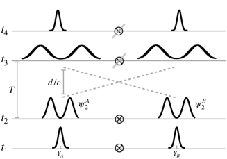
Figure 1: A sketch of the protocol. The particles start in a separable, well-localised state at $t_{1}$. A more general separable state is prepared by local operations ($t_{2}$). The particles evolve freely for a period $T$, resulting in a possibly entangled state. Finally, local operations on the particles make them localised again, without changing the entanglement.

Action —

We assume linearized gravity. For brevity, the metric perturbation $h_{\mu\nu}$ at a fixed time is denoted as $\varphi$ and a ‘path’ $h_{\mu\nu}(t)$ as $\mathcal{G}$. The action of the joint system of field and the two particles $A$ and $B$ is of the form

$$S\left[x_{a},\mathcal{G}\right]=S_{\text{G}}\left[x_{a},\mathcal{G}\right]+\sum_{a\in\{A,B\}}S_{a}\left[x_{a}\right]$$ (1)

where $a=A,B$, $S_{a}$ the action of a particle with mass $m_{a}$ in flat spacetime, and $S_{\text{G}}$ the gravitational action which includes the kinetic terms for $\varphi$ and its coupling to the energy momentum tensor, which in turn describes point particles with trajectories ${x_{a}^{\mu}=(t,\mathbf{x}_{a})}$. $S_{a}$, $S_{\text{G}}$ and $T_{\mu\nu}$ are given in the Appendix. Note that without the term $S_{\text{G}}$ there can be no entanglement generation since $e^{i\sum_{a}S_{a}\left[x_{a}\right]/\hbar}=\prod_{a}e^{iS_{a}\left[x_{a}\right]/\hbar}$.

Path integral — We model the system by a quantum state $\ket{\Psi(t)}\in\mathcal{H}_{A}\otimes\mathcal{H}_{B}\otimes\mathcal{H}_{\text{G}}$, where $\mathcal{H}_{A}$ and $\mathcal{H}_{B}$ are associated with the centre of mass of the particles and $\mathcal{H}_{\text{G}}$ contains the states of the gravitational field. The specific assignment of a state to the gravitational field is a delicate point which we discuss further below.

The state at time $t_{1}$ is assumed to be of the form

$$\ket{\Psi(t_{1})}=\ket{\psi^{A}_{1}}\ket{\psi^{B}_{1}}\ket{\varphi_{1}},$$ (2)

that is, a separable state of the two particles and the field. We also assume that the state at time $t_{4}$ is

$$\ket{\Psi(t_{4})}=U\ket{\Psi(t_{1})}=\ket{\psi_{4}}\ket{\varphi_{1}},$$ (3)

where $U$ is the unitary evolution operator and now $\ket{\psi_{4}}$ is a possibly non-separable state for the two particle, allowing for gravity mediated entanglement.

Note that we have assumed that the state of the gravitational field is the same at the beginning and at the end of the experiment, for two reasons. First, because the particles are light and slow-moving, we assume that the amplitude to excite radiation is negligible; in other words, we approximate the final state as its zero graviton component. Secondly, we assume that the particles start and end in well-localised states at the same position. We take $\ket{\varphi_{1}}$ to be the classical-like state peaked on the classical field $\varphi_{1}$: the newtonian field of two localised particles at $\mathbf{Y}_{A}$ and $\mathbf{Y}_{B}$.

We introduce the path integral by positing that

$$\bra{\mathbf{y}_{4}^{a},\varphi_{1}}{U}\ket{\mathbf{y}_{1}^{a},\varphi_{1}}=\int_{\mathbf{y}_{1}^{a},\varphi_{1}}^{\mathbf{y}_{4}^{a},\varphi_{1}}\text{D}x^{\prime}_{a}\text{D}\mathcal{G^{\prime}}e^{iS[x^{\prime}_{a},\mathcal{G^{\prime}}]},$$ (4)

where $\ket{\mathbf{y}^{a}}$ is a position eigenstate for particle $a.$ Therefore the wavefunction for the final state ${\psi_{4}(\mathbf{y}_{4}^{a}):=\braket{\mathbf{y}^{a}_{4}}{\psi_{4}}}$ is given in terms of the initial wavefunctions ${\psi^{a}_{1}(\mathbf{y}^{a}_{1}):=\braket{\mathbf{y}^{a}_{1}}{\psi^{a}_{1}}}$ as

$$\!\!\!\!\ \psi_{4}(\mathbf{y}_{4}^{a})=\int\mathrm{d}\mathbf{y}_{1}^{a}\psi_{1}^{a}(\mathbf{y}_{1}^{a})\int_{\mathbf{y}_{1}^{a},\varphi_{1}}^{\mathbf{y}_{4}^{a},\varphi_{1}}\text{D}x^{\prime}_{a}\text{D}\mathcal{G^{\prime}}e^{iS[x^{\prime}_{a},\mathcal{G^{\prime}}]}.$$ (5)

We now take the stationary phase approximation for $\mathcal{G}$. The action is to be evaluated on the classical gravitational field $\mathcal{G}[x_{a}]$ sourced by a particle moving as $x_{a}(t)$.

$$\psi_{4}(\mathbf{y}_{4}^{a})\approx\int\mathrm{d}\mathbf{y}_{1}^{a}\psi_{1}(\mathbf{y}_{1}^{a})\int_{\mathbf{y}_{1}^{a}}^{\mathbf{y}_{4}^{a}}\text{D}x^{\prime}_{a}e^{iS[\mathcal{G}[x^{\prime}_{a}]]}.$$ (6)

We have introduced the notation ${S[\mathcal{G}[x^{\prime}_{a}]]=S[x^{\prime}_{a},\mathcal{G}[x^{\prime}_{a}]]}$ for brevity. Note that, in general, ${\mathcal{G}[x^{\prime}_{a}](t_{1})\neq\varphi_{1}\neq\mathcal{G}[x^{\prime}_{a}](t_{4})}$, therefore the path $\mathcal{G}[x^{\prime}_{a}]$ is not one of the paths integrated over in (5). However, we assume for the moment that the error is not too significant, because the initial state will be very localized. The validity of this assumption will be corroborated by our results.

A second stationary phase approximation for the trajectories is taken by keeping only the contribution on the solution of the classical equations of motion for the particles for initial and final positions $\mathbf{y}_{1}^{a}$ and $\mathbf{y}_{4}^{a}$, denoted as $x_{a}$. We obtain that

$$\psi_{4}(\mathbf{y}_{4}^{a})\approx\int\mathrm{d}\mathbf{y}_{1}^{a}\psi_{1}(\mathbf{y}_{1}^{a})e^{iS[\mathcal{G}[x_{a}]]}.$$ (7)

Since $\psi_{1}(\mathbf{y}_{1}^{a})$ is separable in $A$ and $B$, entanglement generation will arise from the $S_{G}$ part of $S$. The gravitational contribution at each $\mathbf{y}_{4}^{a}$ corresponds to a phase ${S_{G}[\mathcal{G}[x_{a}]]}$ with ${x_{a}(t_{1})=\mathbf{y}_{1}^{a}}$ and ${x_{a}(t_{4})=\mathbf{y}_{4}^{a}}$. Each such pair of trajectories sources a gravitational field, and integrating over $\mathbf{y}_{1}^{a}$ corresponds to ‘summing’ the contributions from the gravitational interaction of all these pairs of trajectories for $A$ and $B$.

We note two points that will be further discussed later. First, (7) indicates that the gravitational field is not in a classical-like state during the experiment. Second, the trajectories $x_{a}$ can be taken to be straight lines even when going to the leading order in $1/c$, which indicates no radiation due to no acceleration. This justifies our original assumption of no radiation in $\ket{\varphi_{1}}$.

State evolution —

We have yet to use the assumptions that the ‘splitting’ and ‘recombination’ phases are fast with respect to $T$, which imply we only need to consider the free evolution for $t\in[t_{2},t_{3}]$. It can be shown that, to leading order in $1/c$,

$$\psi_{4}(\mathbf{y}_{4}^{a})\approx \int\mathrm{d}\mathbf{y}_{3}^{a}e^{iS_{3}[\mathcal{G}[x_{3}^{a}]]}\cdot\int\mathrm{d}\mathbf{y}_{2}^{a}e^{iS_{2}[\mathcal{G}[x_{2}^{a}]]}$$

$$\cdot\int\mathrm{d}\mathbf{y}_{1}^{a}\psi_{1}(\mathbf{y}_{1}^{a})e^{iS_{1}[\mathcal{G}[x_{1}^{a}]]}.$$ (8)

$x_{i}^{a}$ are the trajectories of the particles at the time interval $[t_{i},t_{i+1}]$. Above, the actions are approximated up to leading order in $1/c$ (which is $1/c^{2}$). We caution that due to retardation it is not straightforward to arrive at (State evolution —), see the Appendix.

Evolution from $\psi_{2}$ to $\psi_{3}$ is done by the second integral in (State evolution —). The assumptions made previously imply that the evolution done with the actions $S_{1}$ and $S_{3}$ will not contribute to the entanglement measured for $\psi_{4}$. We thus assume that the state $\psi_{2}=\int\mathrm{d}\mathbf{y}_{1}^{a}\psi_{1}e^{iS_{1}}$ has been prepared separable in $A$ and $B$ and write

$$\psi_{3}(\mathbf{y}_{3}^{a})\approx\int\mathrm{d}\mathbf{y}_{2}^{a}e^{iS_{2}[\mathcal{G}[x_{2}^{a}]]}\psi_{2}(\mathbf{y}_{2}^{a}).$$ (9)

Once $\psi_{3}(\mathbf{y}_{3}^{a})$ is calculated, we proceed to compute the entanglement in $\psi_{3}$, which in the approximation we work in will be the same as that in $\psi_{4}$.

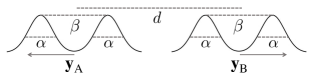
Figure 2: The initial state of matter. We take the convention that the two particles have opposite positive directions to reduce the number of sign changes in what follows. Note that $\omega\equiv\hbar/m\alpha^{2}$.

Two gaussians in path superposition —

We now fix the states $\psi_{2}^{a}$ and apply the above to the generalised case shown in Fig. 2 to arrive at an analytical expression for the entanglement at zeroth order in $1/c$. That is, in this (and the next) section the gravitational interaction is approximated as an instantaneous interaction through a newtonian potential. The state $\psi_{2}=\otimes_{a}\psi_{2}^{a}$ is separable in $A$ and $B$ and describes two quantum particles of mass $m_{a}=m$, each prepared initially in a spatial superposition of two gaussians. The initial wavefunction of each particle in the position basis is

$$\!\!\!\psi^{a}_{2}(\mathbf{y}^{a})\propto\exp\left(-\frac{(\mathbf{y}^{a}-\beta/2)^{2}}{2\alpha^{2}}\right)+\exp\left(-\frac{(\mathbf{y}^{a}+\beta/2)^{2}}{2\alpha^{2}}\right),$$ (10)

where $\alpha$ is the delocalization of the position of each path and $\beta$ is the separation between the two paths. The normalisation will drop out from the entanglement. Thinking of the gaussians as ground states of a harmonic potential (which was turned off at $t=t_{2}$), we introduce the (nominal) frequency $\omega=\hbar/m\alpha^{2}$.

We can calculate $\psi_{3}$ using (9). To simplify the difficult calculation, we assume $d\gg\beta,\alpha,\alpha\omega t$, and expand to second order in the dimensionless parameters $\alpha/d$ and $\beta/d$. This is a realistic assumption for most realistic experimental scenarios. We also expand to zeroth order in the dimensionless parameter $\omega d/c$. The above make the integrals over $\text{d}\mathbf{y}_{2}^{a}$ in (9) computationally tractable. The integrands become sums of gaussians multiplied by polynomials, a case for which closed formulas can be found. The code used for the long analytical calculation is provided as Supplementary Material.

To quantify the amount of entanglement generated by gravity in $\psi_{3}$, we compute the generalised entanglement measure $\mathcal{E}$ recently introduced in [20] and given in the Appendix. This is a generalization to the case of continuous sets of states of the concurrence, a well known entanglement measure for discrete sets of states. We find

$$\mathcal{E}= \frac{2Gm^{2}t}{\hbar d}\frac{1}{d^{2}}\Biggl{[}\frac{1}{4}\beta^{4}+\alpha^{2}\beta^{2}\left(1+\frac{1}{4}(\omega t)^{2}\right)$$ (11)

$$+\alpha^{4}\biggl{[}f_{0}\left(\frac{\beta}{\alpha}\right)+f_{2}\left(\frac{\beta}{\alpha}\right)\frac{(\omega t)^{2}}{3}+f_{4}\left(\frac{\beta}{\alpha}\right)\frac{(\omega t)^{4}}{9}\biggr{]}\Biggr{]}^{1/2}.$$

The functions $f_{0},f_{2}$, and $f_{4}$ are of order unity and given in the appendix. As is shown below, the faster than linear scaling with time is due to the growth in uncertainty.

Path and oscillator protocols —

When $\beta\gg\alpha$ each of the particles begins in a superposition of two gaussians with negligible overlap. This will remain true during the experiment so long as $\beta\gg\alpha\omega T$. Then, (11) reduces to the path protocol entanglement [13]

$$\mathcal{E}_{\beta\gg\alpha}=\frac{Gm^{2}T}{\hbar d}\left(\frac{\beta}{d}\right)^{2}.$$ (12)

When $\beta\ll\alpha$ each particle state is approximately a single gaussian and (11) reduces to

$$\mathcal{E}_{\beta\ll\alpha}=\frac{Gm^{2}T}{\hbar d}\left(\frac{\sqrt{2}\alpha}{d}\right)^{2}\sqrt{1+\frac{(\omega T)^{2}}{3}+\frac{(\omega T)^{4}}{9}}.$$ (13)

We see that the distance $\beta$ between the paths in the path protocol is replaced by the initial gaussian width $\alpha$. The oscillator protocol has an additional amplification term that depends on $\omega T$. When $\omega T$ is large, we obtain

$$\mathcal{E}_{\beta\ll\alpha}^{\omega T\gg 1}=\frac{2}{3}\frac{Gm^{2}T}{\hbar d}\left(\frac{\alpha\omega T}{d}\right)^{2},$$ (14)

which is in accordance with previous literature on the oscillator protocol [4]. Recall that $\omega\propto\alpha^{-2}.$ This means that, while in the small $\omega T$ limit, larger $\alpha$ leads to larger entanglement, in the large $\omega T$ limit, smaller spread leads to larger entanglement. This was already remarked in [4].

Relativistic correction —

We now report the leading correction in $1/c$ for the oscillator protocol when $\omega T\gg 1$. The newtonian potential is now replaced by a Liénard-Wiechert type [17], approximated to leading order in $1/c$. The tedious calculation is given in the Supplementary Material. As in the previous section, we expand the action to second order in $\alpha/d$, but, this time keep the leading order in $\omega d/c$. The state at $t_{2}$ is now

$$\psi_{2}(\mathbf{y}_{a})=\otimes_{a}\psi_{2}^{a}(\mathbf{y}_{a})\propto\otimes_{a}\exp\left(-\frac{{\mathbf{y}^{a}}^{2}}{2\alpha^{2}}\right).$$ (15)

The entangled state $\psi_{3}$ is computed again through (9) and is given in the Supplementary Material. The entanglement is $\mathcal{E}_{\beta\ll\alpha}^{\omega T\gg 1}+\Delta\mathcal{E}_{\beta\ll\alpha}^{\omega T\gg 1}$ with

$$\Delta\mathcal{E}_{\beta\ll\alpha}^{\omega T\gg 1}=-\frac{3}{2}\left(\frac{d}{ct}\right)^{2}\mathcal{E}_{\beta\ll\alpha}^{\omega T\gg 1}.$$ (16)

Using (14), $\Delta\mathcal{E}_{\beta\ll\alpha}^{\omega t\gg 1}$ scales with $(\omega d/c)^{2}$. Note that there will be less entanglement due to this relativistic effect. The correction for general values of $\omega T$ is given in the Appendix.

There is a physical explanation for this, namely, the fact that when $\omega t\gg 1$ the entanglement generation is not due to the initial spread per se, but, due to the fast growth of the spread with free evolution. The particles see each other with retardation and so they see a smaller spread of the other particle, which results in less entanglement. The amount of entanglement reduction is controlled by the ratio of the distance of the center of mass and the light crossing time.

Gravitational attraction —

Feynman imagined detecting the gravitational field of a mass in superposition by measuring the displacement of another mass. However, surprisingly, gravity mediated entanglement can arise with no measurable displacement. This has been the main insight from the path protocol [2, 3]. Owing to our path integral formalism, we can conclude that this is the case for the oscillator protocol too.

To see this, we compare the results of using (i) straight lines trajectories with (ii) the accelerated trajectories of the Kepler problem for the particles. One gets the exact same results at leading order in $1/c$ both for the entanglement (11) and all derived results, as well as for the relativistic correction (16). Therefore at this level of approximation, the entanglement in the oscillator protocol, like that in the path-protocol, is not due to the gravity induced displacement between the particles.

Superposition of geometries —

Let us now return to (7) and discuss the state of the field. For the scope of this computation, we assume that the state of the field is the same at the beginning and at the end of the experiment. In the evaluation of the path integral, we take both the particles and the fields to be on-shell. The picture that arises, to this approximation, is that of a superposition of point particles on constant-velocity trajectories sourcing a corresponding gravitational field. Different trajectories of the particles will source diffeomorphically inequivalent geometries. Additionally, since the trajectories of the particles can be taken to not be accelerated, these geometries do not contain radiation. Therefore we may say that during the experiment, spacetime is in a superposition of a continuum of different, radiation-free, geometries. We may approximate the state of the particles and field at times $t\in[t_{2},t_{3}]$ as

$$\ket{\Psi(t)}\approx\int\mathrm{d}\mathbf{y}^{a}\,\psi(\mathbf{y}^{a})\ket{\mathbf{y}^{a}}\ket{\varphi(\mathbf{y}^{a})},$$ (17)

where $\psi(\mathbf{y}^{a})$ is given by (9), and $\ket{\varphi(\mathbf{y}^{a})}$ are semiclassical states of the fields, peaked on classical fields $\varphi(\mathbf{y}^{a})$ sourced by particles at positions $\mathbf{y}^{a}$.

Conclusions —

We considered a protocol (see Figs. 1 and 2) that generalises the path and oscillator protocols for gravity mediated entanglement. We calculated the newtonian limit entanglement for this protocol in (11) and saw that the path and oscillator protocol entanglement are recovered as physical subregimes in (12) and (13). This is the first indication that entanglement in the oscillator and path protocols is due to superposition of spacetime geometries.

The oscillator and path protocols amount to specific choices for the $\psi^{a}_{2}$ wavefunctions for particles $a=A,B$ in (9) (a sum of Dirac deltas for the path protocol and gaussians for the oscillator protocol). Note that (9) and the general setup and procedure used is applicable to more general (continuous or discrete) prepared wavefunctions $\psi^{a}_{2}$. We see that the final matter state will be entangled in $A$ and $B$ because different trajectories $x_{a}$ of the particles source a different classical field and give rise to a different phase in (9).

Our computation relies on two approximations typical for GME experiments. One of them is $\alpha/d\ll 1$, meaning that the size of each wavefunction is much smaller than the distance between the two. Another approximation is that $\omega d/c\ll 1$, which means that the experiment’s time scales $T,1/\omega$ are long enough relative to the distance scales $d,\alpha$ such that relativistic effects are negligible. The saddle-point approximation is expected to be valid as long as typical values of the action are much larger than $\hbar$.

Another assumption in our computation is that the initial and final states of the particles are very localised, and that therefore they are disentangled from the field. Of course, even though much harder to identify experimentally, detecting gravitationally induced decoherence due to entanglement with the field [21] would in itself be a great feat.

Using the path integral formalism, rather than treating the problem as a direct Hamiltonian interaction term as in [4, 15, 13], allows us to work with covariant quantities: the actions that feature in the entangling phases in (7) and (9). Thus, in this setting, entanglement is generated in a spacetime-local manner. It follows that if the entire protocol lasts for about time $T$ and $T\ll d/c$ the particles will not become entangled. This was shown by some of us for the path protocol in [17]. In this work, we applied a similar computational technique to more general wavefunctions.

We reported in (16) the first correction in $1/c$ for the oscillator entanglement (13) for the case $\omega t\gg 1$. In this case the entanglement is generated due to the fast rate of growth of the spread and scales inversely with the initial spread $\alpha$, as noticed in [4]. The relativistic correction we calculated here intuitively corresponds to the particles seeing each other in the past due to retardation and thus interacting with a gaussian with smaller spread. This gives rise to a negative correction with respect to the newtonian calculation, that is, less entanglement. The relative error of the correction versus the newtonian entanglement is $-\frac{3}{2}\left(d/cT\right)^{2}$. This relativistic correction is very difficult to detect for gravity, but, it could potentially be observed in an electromagnetic version of the experiment.

Our results for the oscillator protocol without relativistic corrections match those of [4]. Relativistic corrections to the entanglement in the oscillator protocol were also computed in [15], but for a slightly different setup. While we compute the entanglement of an initially separable state as a function of interaction time, they compute the entanglement in the joint ground state of gravity and optically-trapped massive particles. As a result, their entanglement does not depend on time. The time-dependence shown here could be exploited in an experimental configuration that starts in two separable oscillator states and introduces the wanted interaction at a later time, e.g. by bringing the particles more closely together.

It has been previously argued by some of us in [16, 17, 25, 18] that the path protocol would show that the gravitational field has been indirectly detected in a quantum superposition of macroscopically distinct geometries. An analogous understanding for continuous matter wavefunctions sourcing the gravitational field has thus far been missing. We have shown here that the entanglement in the oscillator protocol can also be attributed to a superposition of geometries, specifically a superposition of a continuum of different, radiation-free geometries, and the different phases these accrue.

A clear takeaway from our analysis is that if linearised quantum gravity is assumed, whatever the field state is taken to be, it cannot be a classical-like state that approximately solves Einstein’s equations.

Appendix

Action — The metric tensor is approximated as ${{g_{\mu\nu}=\eta_{\mu\nu}+h_{\mu\nu}}}$ where $h_{\mu\nu}$ is the metric perturbation that satisfies $|h_{\mu\nu}|\ll 1$ and $\eta_{\mu\nu}$ is the flat metric. The signature is $(-,+,+,+)$ and we have: $g=\det g_{\mu\nu}$, $t$ the coordinate time, $R$ the Ricci scalar, $G$ Newton’s gravitational constant, $c$ the speed of light, and $x_{a}^{\mu}=(ct,\mathbf{x}_{a}(t))$ the trajectory of particle $a$. We have

$$S_{a}[x_{a}]=-m_{a}c\int\text{d}t\sqrt{-\eta_{\mu\nu}\dot{x}_{a}^{\mu}\dot{x}_{a}^{\nu}},$$ (18)

$$S_{\text{G}}\left[x_{a},g\right]= \int\text{d}^{4}x\frac{c^{3}}{16\pi G}[\sqrt{-g}R]_{\mathcal{O}(h_{\mu\nu}^{2})}$$ (19)

$$-\int\text{d}^{4}x\frac{1}{2c}h_{\mu\nu}T^{\mu\nu}\big{|}_{g_{\mu\nu}=\eta_{\mu\nu}}+O(h_{\mu\nu}^{3}),$$

and

$$T^{\mu\nu}\big{|}_{g=\eta}=\sum_{a}\gamma_{a}(t)m_{a}\dot{x}_{a}^{\mu}\dot{x}_{a}^{\nu}\delta^{(3)}(\mathbf{x}-\mathbf{x}_{a}).$$ (20)

Note that taking only the interaction term $\sim T_{\mu\nu}h^{\mu\nu}$ of $S_{\text{G}}$ would give a wrong numerical result by a factor of two as the contribution of the kinetic terms of $h_{\mu\nu}$ also need to be taken into account. The on-shell action $\tilde{S}_{\text{G}}$ reads [17]

$$S_{\text{G}}[\mathcal{G}[x^{\prime}_{a}]]= \sum_{a\neq b}\int_{0}^{t}\text{d}t^{\prime}\frac{Gm_{a}m_{b}\bar{V}_{a}^{\mu\nu}(t_{ab})V_{b\mu\nu}/c^{4}}{d_{ab}^{\mu}\dot{x}^{\prime}_{a\mu}(t_{ab})/c},$$ (21)

with

$$V_{a}^{\mu\nu} =\dot{x}_{a}^{\mu}\dot{x}_{a}^{\nu}/\sqrt{\dot{x}_{a}^{\mu}\dot{x}_{a}^{\nu}\eta_{\mu\nu}/c^{2}},$$ (22)

$$\bar{V}^{\mu\nu} =V^{\mu\nu}-\frac{1}{2}\eta^{\mu\nu}\eta_{\alpha\beta}V^{\alpha\beta},$$ (23)

$$d_{ab}^{\mu}\equiv x_{b}^{\mu}-x_{a}^{\mu}( t_{ab})=(ct-ct_{ab},\mathbf{x}_{b}-\mathbf{x}_{a}(t_{ab})),$$ (24)

where $t_{ab}$ is the retarded time, defined implicitly as ${d_{ab}^{2}=0}$. The omitted time argument in $V_{a\mu\nu},d_{ab},\mathbf{x}_{a}$ and $x_{a}^{\mu}$ implies dependence on the non-retarded time $t^{\prime}$.

Path integral at leading order in $1/c$ — We split the path integral at times $t_{2},t_{3}$ as

$$\psi_{4}(\mathbf{y}_{4}^{a})= \int\mathrm{d}\mathbf{y}_{3}^{a}\int\mathrm{d}\mathbf{y}_{2}^{a}\int\mathrm{d}\mathbf{y}_{1}^{a}\psi_{1}(\mathbf{y}_{1}^{a})$$ (25)

$$\int_{\mathbf{y}_{1}^{a}}^{\mathbf{y}_{2}^{a}}\text{D}x_{1}^{a}e^{iS_{1}[\mathcal{G}[x_{1}^{a}]]}\int_{\mathbf{y}_{2}^{a}}^{\mathbf{y}_{3}^{a}}\text{D}x_{2}^{a}e^{iS_{2}[\mathcal{G}[x_{1}^{a},x_{2}^{a}]]}$$

$$\int_{\mathbf{y}_{3}^{a}}^{\mathbf{y}_{4}^{a}}\text{D}x_{3}^{a}e^{iS_{3}[\mathcal{G}[x_{1}^{a},x_{2}^{a},x_{3}^{a},]]}.$$

where the path $x_{i}$ connects $y_{i}$ and $y_{i+1}$. Note that, because of the retardation of the field, $S_{2}$ and $S_{3}$ depend on the path in the previous time interval. This dependence can be disregarded to leading order in $1/c$, since the time interval influenced by the previous trajectory is then of order $d/c$, which implies that the contribution of the previous trajectories will be one order higher in $1/c$.

Schematically, we approximate the action in interval $i$ as

$$S_{i} =\int_{t_{i}}^{t_{i+1}}L_{[-\infty,t^{\prime}]}\mathrm{d}t^{\prime}\approx\int_{t_{i}}^{t_{i+1}}L_{[t^{\prime}-d/c,t^{\prime}]}\mathrm{d}t^{\prime}$$ (26)

$$=\int_{t_{i}}^{t_{i}+d/c}L_{[t^{\prime}-d/c,t^{\prime}]}\mathrm{d}t^{\prime}+\int_{t_{i}+d/c}^{t_{i+1}}L_{[t^{\prime}-d/c,t^{\prime}]},\mathrm{d}t^{\prime}$$

where $L_{[t^{\prime},t^{\prime\prime}]}$ depends on the particle trajectories between times $t^{\prime}$ and $t^{\prime\prime}$. Now, notice that in the first term the integration is over a time interval of length $d/c$. This implies that the contribution from that term will be one order higher in $1/c$ than the second term, meaning we can neglect it. Therefore, after a simple change of variables, we may write

$$S_{i} \approx\int_{t_{i}}^{t_{i+1}-d/c}L_{[t^{\prime},t^{\prime}+d/c]}.$$ (27)

Thus $S_{i}$ only depends on the particle trajectories between $t_{i},t_{i+1}$. This way, we can neglect the dependence of $S_{2}$ and $S_{3}$ on the past of the trajectories and write $S_{3}[\mathcal{G}[x_{1}^{a},x_{2}^{a},x_{3}^{a}]]\approx S[\mathcal{G}[x_{3}^{a}]]$ and $S_{2}[\mathcal{G}[x_{1}^{a},x_{2}^{a}]]\approx S[\mathcal{G}[x_{2}^{a}]]$.

Entanglement measure — The definition of $\mathcal{E}$ for a normalized bi–partite pure state $\ket{\psi}$ is [20]

$$\mathcal{E}^{2}=2-2\int\text{d}y_{1}\text{d}y^{\prime}_{1}\left|\int\text{d}y_{2}\psi(y_{1},y_{2})\psi^{*}(y^{\prime}_{1},y_{2})\right|^{2}.$$ (28)

The functions $f_{0}$,$f_{2}$,$f_{4}$ — The functions from Eq. (11) are order unit and given by

$$f_{0}(x) =\frac{-x^{4}-4x^{2}+4e^{x^{2}/2}-2e^{x^{2}/4}(x^{4}+2x^{2}-4)+4}{4(e^{x^{2}/4}+1)^{2}}$$ (29)

$$f_{2}(x) =\frac{-12x^{2}+8e^{x^{2}/2}+(-3x^{4}-12x^{2}+16)e^{x^{2}/4}+8}{8(e^{x^{2}/4}+1)^{2}}$$

$$f_{4}(x) =\frac{(-x^{2}/2+e^{x^{2}/4}+1)^{2}}{(e^{x^{2}/4}+1)^{2}}$$

They are plotted in the Supplementary Material.

Relativistic correction — The relativistic correction to (13) for general values of $\omega T$ was found to be

$$\Delta\mathcal{E}_{\beta\ll\alpha}= -\frac{1}{2}\left(\frac{\omega d}{c}\right)^{2}\frac{Gm^{2}T}{\hbar d}\left(\frac{\sqrt{2}\alpha}{d}\right)^{2}$$ (30)

$$\times\frac{\left(\omega T\right)^{2}/3-1}{\sqrt{1+\frac{(\omega T)^{2}}{3}+\frac{(\omega T)^{4}}{9}}}.$$

I Supplementary Material

Mathematica notebooks— We give an overview of the computation performed in the Mathematica notebooks published with this work. When descriptions differ, we will refer to the one used to achieve the relativistic corrections as rel and to the one used to calculate the entanglement of paths with uncertainty as path.The notebooks are available under https://github.com/ofek-b/gme_superposition_geometries. We first define three dimesionless quantities: $\phi=\frac{Gm^{2}}{\hbar\omega d}$, which is a measure for the effect of gravity in the system; $\epsilon=\alpha/d$, which is a measure of the quantum uncertainty of the particles’ paths; and $\Omega=\omega d/c$, which is a measure for the effect of retardation in the system. When we write that we expand quantities, it is meant that we perform a series expansion to second order in $\epsilon$ in both computations and to zeroth (second) order in $\Omega$ in paths (rel). Note that in paths we define $\xi=\beta/\alpha$ and so take second order in $\beta/d=\epsilon\xi$ automatically as well.

In rel, we find the retarded time $t_{ab}$ by solving a quadratic equation resulting from expanding its implicit definition $d_{ab}^{2}=0$ with $d_{ab}$ defined in Eq. (24).

We then proceed to expand the action $S[q_{1},q_{2}]=\int_{0}^{t}dt^{\prime}(L_{A}+L_{B}+L_{\text{G}})$, a functional of general trajectories $q_{1}(t),q_{2}(t)$. We use the relativistic kinetic energy for the uncoupled part $L_{A}+L_{B}$ and the on-shell action Eq. (21) for $L_{\text{G}}$. In rel, we introduce the bookkeeping variables ret and kin as follows to keep track of which relativistic contributions result from retardation (i.e., the finite-speed propagation of the change in spacetime’s geometry) and which from kinetic energy and momenta gravitating (i.e., the correction to the sourcing of those changes predicted by GR). Note that this distinction is frame dependent and is not addressed in the main text, but will be used shortly.

$$(L_{A}+L_{B})/\hbar\approx\frac{q_{1}^{\prime}(t)^{2}+q_{2}^{\prime}(t)^{2}}{2\omega}+\frac{\Omega^{2}\epsilon^{2}\left(q_{1}^{\prime}(t)^{4}+q_{2}^{\prime}(t)^{4}\right)}{8\omega^{3}}-\frac{2\omega}{\Omega^{2}\epsilon^{2}},$$

$$L_{\text{G}}/\hbar\approx \omega\epsilon^{2}\phi(q_{1}(t)+q_{2}(t))^{2}-\omega\epsilon\phi(q_{1}(t)+q_{2}(t))+\omega\phi$$

$$+\text{kin}\left(-\frac{4\Omega^{2}\epsilon^{2}\phi q_{1}^{\prime}(t)q_{2}^{\prime}(t)}{\omega}+\frac{3\Omega^{2}\epsilon^{2}\phi q_{1}^{\prime}(t)^{2}}{2\omega}+\frac{3\Omega^{2}\epsilon^{2}\phi q_{2}^{\prime}(t)^{2}}{2\omega}\right)$$

$$+\text{ret}^{2}\left(\frac{\Omega^{2}\epsilon\phi\left(q_{1}^{\prime\prime}(t)+q_{2}^{\prime\prime}(t)\right)}{2\omega}-\frac{2\Omega^{2}\epsilon^{2}\phi q_{1}^{\prime}(t)q_{2}^{\prime}(t)}{\omega}+\frac{\Omega^{2}\epsilon^{2}\phi q_{1}^{\prime}(t)^{2}}{\omega}+\frac{\Omega^{2}\epsilon^{2}\phi q_{2}^{\prime}(t)^{2}}{\omega}\right)$$

$$+\text{ret}\left(-\frac{\Omega^{2}\epsilon\phi\left(q_{1}^{\prime\prime}(t)+q_{2}^{\prime\prime}(t)\right)}{4\omega}+\frac{\Omega^{2}\epsilon^{2}\phi q_{1}^{\prime}(t)q_{2}^{\prime}(t)}{\omega}-\frac{\Omega^{2}\epsilon^{2}\phi q_{1}^{\prime}(t)^{2}}{2\omega}-\frac{\Omega^{2}\epsilon^{2}\phi q_{2}^{\prime}(t)^{2}}{2\omega}\right).$$

The Lagrangian of paths (this of a Newtonian two-body problem) is achieved for kin, ret, $\Omega\rightarrow 0$. The Lagrangian of GR up to leading order in $1/c$ is achieved for taking both kin $=$ ret $=1$:

$$L_{\text{G}}/\hbar\approx \omega\epsilon^{2}\phi(q_{1}(t)+q_{2}(t))^{2}-\omega\epsilon\phi(q_{1}(t)+q_{2}(t))+\omega\phi+\frac{\Omega^{2}\epsilon\phi}{\omega}\left(\frac{q_{1}^{\prime\prime}(t)+q_{2}^{\prime\prime}(t)}{4}-5\epsilon q_{1}^{\prime}(t)q_{2}^{\prime}(t)+8\epsilon q_{1}^{\prime}(t)^{2}+2\epsilon q_{2}^{\prime}(t)^{2}\right)$$

The classical trajectories beginning at $\mathbf{y}^{\prime}_{a}$ and ending at $\mathbf{y}_{a}$ at time $t$ for the system are then calculated by solving the Euler-Lagrange equations resulting from the action. In rel, we first solve the non-relativistic equations of motion to achieve $\tilde{x}_{a}(t)$, and then plug in $q_{a}(t)=\tilde{x}_{a}(t)+\Omega c_{a}(t)$ to the relativistic equations of motion. We expand them and then solve for the correction $c_{a}(t)$. As it turns out, at the order of our expansion there is no relativistic correction to the classical trajectories. Note that as we have checked, the final result for the entanglement remains the same for both calculations if one takes the classical trajectories to be straight lines. This could be expected on order-of-magnitude grounds.

The trajectories are then plugged into the action and the wavefunction under the stationary phase approximation Eq. (9) is achieved after expanding the integrand and solving the integral. The wavefunction is a sum of polynomials multiplied by gaussians (in rel this sum has a single term, in paths two). Using a closed formula for the moments of the gaussian distribution we are able to perform the integral defining the generalized entanglement measure Eq. (28) as a sum of expectation values of polynomials under a gaussian distribution (one in rel, sixteen in paths). Before solving the integral we expand the polynomials to an order double of the usual one, as ultimately a square root will be taken. We then arrive at our results Eqs. (11), (16). In the latter, we can set only one of kin and rel to one to achieve the different corrections from retardation and kinetic energy and momenta gravitating. We find that each time we get the correction reported in the main text multiplied by a numerical factor: $4/5$ and $1/5$ respectively.

Figure 3: The functions from Eq. (11). They are of order unit. The horizontal axis is $x=\beta/\alpha$.

in 1,…,8 See pages \x of paths.pdf in 1,…,11 See pages \x of rel.pdf

References

- Rickles and DeWitt [2011] D. Rickles and C. M. DeWitt, eds., The Role of Gravitation in Physics: Report from the 1957 Chapel Hill Conference, EOS – Sources (Max-Planck-Gesellschaft zur Förderung der Wissenschaften, Berlin, 2011).
- Bose et al. [2017] S. Bose, A. Mazumdar, G. W. Morley, H. Ulbricht, M. Toroš, M. Paternostro, A. A. Geraci, P. F. Barker, M. S. Kim, and G. Milburn, Spin Entanglement Witness for Quantum Gravity, Physical Review Letters 119, 240401 (2017).
- Marletto and Vedral [2017] C. Marletto and V. Vedral, Gravitationally Induced Entanglement between Two Massive Particles is Sufficient Evidence of Quantum Effects in Gravity, Physical Review Letters 119, 240402 (2017).
- Krisnanda et al. [2020] T. Krisnanda, G. Y. Tham, M. Paternostro, and T. Paterek, Observable quantum entanglement due to gravity, npj Quantum Information 6, 1 (2020).
- Poot and van der Zant [2012] M. Poot and H. S. van der Zant, Mechanical systems in the quantum regime, Physics Reports 511, 273 (2012).
- Aspelmeyer et al. [2014] M. Aspelmeyer, T. J. Kippenberg, and F. Marquardt, Cavity optomechanics, Rev. Mod. Phys. 86, 1391 (2014).
- Gonzalez-Ballestero et al. [2021] C. Gonzalez-Ballestero, M. Aspelmeyer, L. Novotny, R. Quidant, and O. Romero-Isart, Levitodynamics: Levitation and control of microscopic objects in vacuum, Science 374, 10.1126/science.abg3027 (2021), arXiv:2111.05215 .
- Schmöle et al. [2016] J. Schmöle, M. Dragosits, H. Hepach, and M. Aspelmeyer, A micromechanical proof-of-principle experiment for measuring the gravitational force of milligram masses, Classical and Quantum Gravity 33, 125031 (2016), arXiv:1602.07539 .
- Liu et al. [2021] Y. Liu, J. Mummery, and M. A. Sillanpää, Prospects for observing gravitational forces between nonclassical mechanical oscillators, Physical Review Applied 15, 034004 (2021), arXiv:2008.10477 .
- Westphal et al. [2021] T. Westphal, H. Hepach, J. Pfaff, and M. Aspelmeyer, Measurement of gravitational coupling between millimetre-sized masses, Nature 591, 225 (2021).
- Lee et al. [2020] J. G. Lee, E. G. Adelberger, T. S. Cook, S. M. Fleischer, and B. R. Heckel, New Test of the Gravitational Law at Separations down to 52 m, Physical Review Letters 124, 101101 (2020).
- Rijavec et al. [2021] S. Rijavec, M. Carlesso, A. Bassi, V. Vedral, and C. Marletto, Decoherence effects in non-classicality tests of gravity, New Journal of Physics 23, 043040 (2021), arXiv:2012.06230 .
- Aspelmeyer [2022] M. Aspelmeyer, When Zeh Meets Feynman: How to Avoid the Appearance of a Classical World in Gravity Experiments, in From Quantum to Classical, Vol. 204, edited by C. Kiefer (Springer International Publishing, Cham, 2022) pp. 85–95.
- Yant and Blencowe [2023] J. Yant and M. Blencowe, Gravitational Harmonium: Gravitationally Induced Entanglement in a Harmonic Trap (2023), arXiv:2302.05463 .
- Bose et al. [2022] S. Bose, A. Mazumdar, M. Schut, and M. Toroš, Mechanism for the quantum natured gravitons to entangle masses, Physical Review D 105, 106028 (2022).
- Christodoulou and Rovelli [2019] M. Christodoulou and C. Rovelli, On the possibility of laboratory evidence for quantum superposition of geometries, Physics Letters B 792, 64 (2019), arXiv:1808.05842 .
- Christodoulou et al. [2023a] M. Christodoulou, A. Di Biagio, M. Aspelmeyer, Č. Brukner, C. Rovelli, and R. Howl, Locally Mediated Entanglement in Linearized Quantum Gravity, Physical Review Letters 130, 100202 (2023a).
- Christodoulou et al. [2023b] M. Christodoulou, A. D. Biagio, R. Howl, and C. Rovelli, Gravity entanglement, quantum reference systems, degrees of freedom, Classical and Quantum Gravity 40, 047001 (2023b).
- Chen et al. [2022] L.-Q. Chen, F. Giacomini, and C. Rovelli, Quantum States of Fields for Quantum Split Sources (2022), arXiv:2207.10592 .
- Swain et al. [2022] S. N. Swain, V. S. Bhaskara, and P. K. Panigrahi, Generalized Entanglement Measure for Continuous Variable Systems, Physical Review A 105, 052441 (2022), arXiv:1706.01448 .
- Kanno et al. [2021] S. Kanno, J. Soda, and J. Tokuda, Noise and decoherence induced by gravitons, Physical Review D 103, 044017 (2021), arXiv:2007.09838 .
- Galley et al. [2022] T. D. Galley, F. Giacomini, and J. H. Selby, A no-go theorem on the nature of the gravitational field beyond quantum theory, Quantum 6, 779 (2022).
- Marletto and Vedral [2020] C. Marletto and V. Vedral, Witnessing nonclassicality beyond quantum theory, Physical Review D: Particles and Fields 102, 086012 (2020), arXiv:2003.07974 .
- Di Biagio et al. [2023] A. Di Biagio, R. Howl, Č. Brukner, C. Rovelli, and M. Christodoulou, Relativistic locality can imply subsystem locality (2023), arXiv:2305.05645 .
- Polino et al. [2022] E. Polino, B. Polacchi, D. Poderini, I. Agresti, G. Carvacho, F. Sciarrino, A. Di Biagio, C. Rovelli, and M. Christodoulou, Photonic Implementation of Quantum Gravity Simulator (2022), arXiv:2207.01680 .