TaxAI: A Dynamic Economic Simulator and Benchmark for Multi-Agent Reinforcement Learning

Abstract

Taxation and government spending are crucial tools for governments to promote economic growth and maintain social equity. However, the difficulty in accurately predicting the dynamic strategies of diverse self-interested households presents a challenge for governments to implement effective tax policies. Given its proficiency in modeling other agents in partially observable environments and adaptively learning to find optimal policies, Multi-Agent Reinforcement Learning (MARL) is highly suitable for solving dynamic games between the government and numerous households. Although MARL shows more potential than traditional methods such as the genetic algorithm and dynamic programming, there is a lack of large-scale multi-agent reinforcement learning economic simulators. Therefore, we propose a MARL environment, named TaxAI, for dynamic games involving $N$ households, government, firms, and financial intermediaries based on the Bewley-Aiyagari economic model. Our study benchmarks 2 traditional economic methods with 7 MARL methods on TaxAI, demonstrating the effectiveness and superiority of MARL algorithms. Moreover, TaxAI’s scalability in simulating dynamic interactions between the government and 10,000 households, coupled with real-data calibration, grants it a substantial improvement in scale and reality over existing simulators. Therefore, TaxAI is the most realistic economic simulator, which aims to generate feasible recommendations for governments and individuals.

1 Introduction

The invisible hand [1; 2] of the market is not omnipotent, and in reality, all countries rely on government intervention to promote economic development and maintain social fairness. The extent of government intervention varies from country to country, such as a free market economy [3; 4], planned economies [5; 6] or mixed economies [7; 8; 9]. However, determining the optimal government intervention degree is challenging for several reasons. Firstly, extracting relevant and actionable information from the complex society is arduous. Secondly, governments face difficulties in effectively modeling a vast and heterogeneous population with diverse preferences and characteristics. Lastly, the behavioral response of individuals to incentives remains highly unpredictable.

In this intricate matter of government intervention, we opt to investigate a crucial and efficacious tool, tax policy, which is commonly studied using agent-based modeling (ABM) [10; 11] in economics. ABM is an effective approach to simulate individual behaviors and show the relationship between micro-level decisions and macro-level phenomena. However, traditional ABM suffers from simplicity and subjectivity in setting model parameters and behavior rules, making it difficult to simulate realistic scenarios [12; 11; 13]. While Multi-Agent Reinforcement Learning (MARL) surpasses traditional ABM settings by offering optimal actions based on evolving state information. Some MARL algorithms perform well in partially observable environments and adaptively learn to reach equilibrium solutions [14; 15; 16]. Hence, MARL is well-suited for addressing dynamic game problems involving the government and a large population. However, despite the significant advantages of MARL, there is currently a shortage of large-scale MARL economic simulators designed specifically for the study of tax policies. In the existing literature, the AI Economist [17] and the RBC model [18] emerge as the most closely related simulators to TaxAI. However, these models exhibit certain limitations, notably a partial grounding in economic theory, limited scalability in simulating a significant number of agents, and the absence of calibration using real-world data (as detailed in Table 1). Therefore, proposing a MARL environment for studying optimal tax policies and solving the dynamic game between the government and the population holds significant research and practical value.

Therefore, we introduce a dynamic economic simulator, TaxAI, based on the Bewley-Aiyagari economic model [19; 20], which is widely used to study capital market frictions, wealth distribution, economic growth issues. By incorporating the Bewley-Aiyagari model, TaxAI benefits from robust theoretical foundations in economics and models a broader range of social roles (shown in Figure 1). Based on TaxAI, we benchmark 2 economic methods and 7 MARL algorithms, optimizing fiscal policy for the government, working and saving strategies for heterogeneous households. In our experiments, we compared 9 baselines across four distinct tasks, evaluating them from both macroeconomic and microeconomic perspectives. Our results revealed the tax-avoidance behavior of MARL-based households and the varying saving and working strategies among households with different levels of wealth. Finally, we test the TaxAI environment using 9 baselines with households’ number ranging from 10, 100, 1000, and even up to 10,000, demonstrating its capability to simulate large-scale agents. In summary, our work encompasses the following three contributions:

1. A dynamic economic simulator TaxAI. The simulator incorporates multiple roles and main economic activities, employs real-data calibration, and facilitates simulations of up to 10,000 agents. These features provide a more comprehensive and realistic simulation than existing simulators.

2. Validation of MARL feasibility in optimizing tax policies. We implemented 2 traditional economic approaches and 7 MARL methods to solve optimal taxation for the social planner, and optimal saving and working strategies for households. The results obtained through MARL methods surpass those achieved by traditional methods.

3. Economic analysis of different policies. We conducted assessments from both macroeconomic and microeconomic perspectives, uncovering tax-avoidance behaviors among MARL-based households in their pursuit of maximum utility. Furthermore, we observed distinct strategies among households with differing levels of wealth.

Codes for the TaxAI simulator and benchmark results can be found at https://github.com/jidiai/TaxAI/.

Table 1: A comparison of MARL simulators for optimal taxation problems.

Simulator	AI Economist	RBC Model	TaxAI (ours)
Households’ Number	10	100	10000
Tax Schedule	Non-linear	Linear	Non-linear
Tax Type	Income	Income	Income&Wealth&Consumption
Social Roles’ Types	2	3	4
Saving Strategy	$\times$	✓	✓
Heterogenous Agent	✓	✓	✓
Real-data Calibration	$\times$	$\times$	✓
Open source	✓	$\times$	✓
MARL Benchmark	$\times$	$\times$	✓

2 Related Works

Classic Tax Models

Economic models provide powerful tools for modeling economic activities and explaining economic phenomena. In microeconomics, the Supply and Demand model [21; 22] reveals the mechanism behind market price formation, while the marginal utility theory [23] underscores the significance of consumption decisions. In macroeconomics, the Keynesian Aggregate Demand-Aggregate Supply Model [24; 25] addresses short-term fluctuations and policy effects [26]. The Comparative Advantage Theory [27; 28] in international trade explains collaborations across nations. The Quantity Theory of Money [29; 30] investigates the relationship between money supply and price levels. Regarding the optimal tax problem, the Ramsey-Cass-Koopmans (RCK) model [31; 32] studies the consumption and savings decisions of representative agents but ignoring individual heterogeneity. The Diamond-Mirrlees model [33; 34] considers the role of taxes and labor supply in social welfare but overlooks income and asset taxes. The Overlapping Generations (OLG) model [35] emphasizes intergenerational inheritance and resource transfers [36; 37]. In contrast, the Bewley-Aiyagari model [38; 39] can assess the impact of taxation on growth, wealth distribution and welfare while simulating real-world income disparities and risk-bearing capacity of individuals. This makes the Bewley-Aiyagari model an ideal choice for studying optimal taxation and household strategies.

Traditional Economic Methods

The optimal tax policy and wealth distribution [40] have been extensively studied in economics. Existed works [38; 41] have utilized mathematical programming methods to address decision-making processes related to governments and households [42; 43]. However, these approaches oversimplify decision-makers rationality and fail to consider autonomous learning abilities and environmental uncertainties. In contrast, dynamic programming-based approaches [44; 45] consider long-term consequences and environmental dynamics but struggle to model non-rational behaviors [46]. Alternative approaches, such as empirical rules [47; 48] and Agent-Based Modeling (ABM) [49; 50], have emerged to address these limitations. ABM enables the exploration of micro-level behaviors and their impact on macro-level phenomena, showing in the ASPEN model [51], income distribution [52] and transaction development [53].

MARL and Simulators for Economy

MARL aims to address issues of cooperation [54] and competition [55] among multiple decision-makers [56]. The simplest MARL method Independent Learning [57; 58], including IPPO [59], and IDDPG [60], involves each agent learning and making decisions independently, disregarding the presence of other agents [61]. In the Centralized Training Decentralized Execution (CTDE) algorithms, like MADDPG [62], QMIX [63], and MAPPO [64], agents share information during training but make decentralized decisions during execution to enhance collaborative performance. To address significant computational and communication overhead posed by a growing number of agents [65], Mean-Field Multi-Agent Reinforcement Learning (MF-MARL) [66] simplifies the problem by treating homogeneous agents as distributed particles [67]. On the other hand, Heterogeneous Agent Reinforcement Learning (HARL) [68], HAPPO and HATRPO, is designed to achieve effective cooperation in a general setting involving heterogeneous agents.

Currently, there are not many efforts employing MARL methods to determine optimal tax policies and individual strategies. The closest works to our paper include AI economist [17] and the RBC model [18]. While they both account for fundamental economic activities, they lack large-scale agent simulation, real-data calibration, and MARL benchmarks. These limitations make practical implementation challenging, which is why we introduce TaxAI. However, prior researches have already explored reinforcement learning-based approaches in some subproblems. For instance, in addressing optimal savings and consumption problems, some studies [69; 70; 71] have utilized single-agent RL to model the representative agent or a continuum of agents. Meanwhile, others have employed MARL to solve rational expectations equilibrium [72; 73], optimal asset allocation and savings strategies [74]. Regarding optimal government intervention problems, research has explored the application of RL in investigating optimal monetary policy [75; 76], international trade [77], redistribution systems [78; 79], and the cooperative relationship between central and local governments under COVID-19 [80].

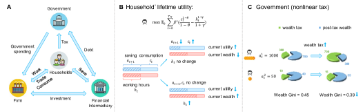
Figure 1: Model Dynamics in the Bewley-Aiyagari Model. A: Economic activities among the government, the firm, the financial intermediary, and households. B: The influence of households’ saving and labor strategies on current utility and wealth. Households must strike a balance between consumption and savings, as well as work and leisure, to optimize lifetime utility. Increasing consumption enhances current utility but reduces current wealth, affecting future utility. Longer working hours yield higher labor income, thereby increasing wealth, but simultaneously result in disutility. C: The effect of government taxation on households’ wealth. The social planner employs a nonlinear taxation, applying varying tax rates based on different assets. As tax rates rise, the taxes paid by households increase, with wealthier household contributing more. This narrows the gap in households’ post-tax wealth, leading to a reduction in the Gini coefficient for wealth distribution.

3 Bewley-Aiyagari Model

In comparison to classical economic models in the related works 2, we contend that the Bewley-Aiyagari model serves as the most suitable theoretical foundation for investigating optimal tax policy for the government and optimal savings and labor strategies for households. In this section, we provide a brief overview of the Bewley-Aiyagari model. This model encompasses four key societal roles: N households, a representative firm, a financial intermediary, and the government. The interactions among them are illustrated in Figure 1. All model variables and their corresponding symbols are organized in Table 5. More details on model assumptions and dynamics are shown in Appendix A.1, A.2.

3.1 $N$ Households

To avoid differences in age, gender, and personality, individuals are modeled as households, whose main activities of households including production, consumption, savings, and tax payments. First of all, households’ income is derived from two sources. They work in the technology firm for the labor income $W_{t}e_{t}h_{t}$, which depends on the wage rate $W_{t}$, the individual labor productivity levels $e_{t}$ and the working hours $h_{t}$. On the other hand, households can only engage in savings and are assumed not to borrow($a_{t}\geq 0$). They earn interest income $r_{t-1}a_{t}$ from savings, which depends on household asset $a_{t}$ and the return to savings $r_{t-1}$.

$$i_{t}=W_{t}e_{t}h_{t}+r_{t-1}a_{t}$$ (1)

In this model, $N$ households are heterogeneous in terms of labor productivity levels $e_{t}$ and initial asset $a_{0}$, and we model $e_{t}$ as either being in a super-star ability or a normal state. In the normal state, it follows an AR(1) process,

$$\log e_{t}=\rho_{e}\log e_{t-1}+\sigma_{e}u_{t}$$ (2)

where $\rho_{e}$ is the persistence and $\sigma_{e}$ is the volatility of the standard normal shocks $u_{t}$. In the super-star state, the labor market ability is $\bar{e}$ times higher than the average. The transition of households from the normal state to the super-star state occurs with a constant probability $p$ while remaining in the super-star state has a constant probability $q$.

In addition, each household seeks to maximize lifetime utility 3 depends on consumption $c_{t}$ and working hours $h_{t}$, subject to budget constraint, where $\beta$ is the discount factor, $\theta$ is the coefficient of relative risk aversion (CRRA), and $\gamma$ represents the inverse Frisch elasticity. $T_{N}$ denotes the maximum steps.

$$\max\quad\mathbb{E}_{0}\sum_{t=0}^{T_{N}}\beta^{t}\left(\frac{c_{t}^{1-\theta}}{1-\theta}-\frac{h_{t}^{1+\gamma}}{1+\gamma}\right)$$ (3)

s.t. $$(1+\tau_{s})c_{t}+a_{t+1}=i_{t}-T(i_{t})+a_{t}-T^{a}(a_{t})$$

The households are required to pay taxes to the government, including consumption taxes $\tau_{s}$, income taxes $T(i_{t})$, and asset taxes $T^{a}(a_{t})$, the last two are expressed by a nonlinear $\mathrm{HSV}$ tax function [48; 81],

$$T\left(i_{t}\right)=i_{t}-(1-\tau)\frac{i_{t}^{1-\xi}}{1-\xi},\quad T^{a}\left(a_{t}\right)=a_{t}-\frac{1-\tau_{a}}{1-\xi_{a}}a_{t}^{1-\xi_{a}}$$ (4)

where $\tau,\tau_{a}$ determine the average level of the marginal income and asset tax, and $\xi,\xi_{a}$ determine the slope of the marginal income and asset tax schedule. It presents a free market economy when all taxes are equal to 0.

3.2 Technology Firm

As the representative of all firms and industries, the firm converts capital and labor into goods and services. We assume it produces a homogeneous good with technology, which can meet the consumption need of households, following the Cobb–Douglas production function,

$$Y_{t}=K_{t}^{\alpha}L_{t}^{1-\alpha}$$ (5)

where $K_{t}$ and $L_{t}$ are capital and labor used for production, $\alpha$ is capital elasticity, and we normalize the output price to 1. The firm rent capital at a rental rate $R_{t}$ and hires labor at a wage rate $W_{t}$. The produced output is used for all households’ gross consumption $C_{t}$, government spending $G_{t}$, and physical capital investment $X_{t}=K_{t+1}-(1-\delta)K_{t}$, with the depreciation rate $\delta$, so the aggregate resource constraint is

$$Y_{t}=C_{t}+X_{t}+G_{t}$$ (6)

Suppose the firm takes the marginal income from labor as households’ wage rate $W_{t}$ and the marginal income from capital as the rental rate $R_{t}$.

$$\begin{split}W_{t}=\frac{\partial Y_{t}}{\partial L_{t}}=(1-\alpha)(\frac{K_{t}}{L_{t}})^{\alpha},\quad R_{t}=\frac{\partial Y_{t}}{\partial K_{t}}=\alpha(\frac{K_{t}}{L_{t}})^{\alpha-1}\end{split}$$ (7)

Market clearing on labor and goods is an important assumption for simplification, which means there is an equilibrium between supply and demand. The goods market clears by Walras’ Law, and the labor market clearing condition is $L_{t}=\sum_{i}^{N}e_{t}^{i}h_{t}^{i}$.

3.3 Government

The government has multiple goals, such as promoting economic growth, maintaining social fairness and stability, and maximizing social welfare. To optimize these objectives, the government typically employs three tools, including government spending $G_{t}$, taxation $T_{t}$, and debt $B_{t}$ with the interest rate $r_{t-1}$. For instance, when optimizing social welfare, the government’s objective and the budget constraint are as follows:

$$\max \quad J=\mathbb{E}_{0}\sum_{t=0}^{\infty}\beta^{t}\left(\sum_{i}^{N}\frac{{c_{t}^{i}}^{1-\theta}}{1-\theta}-\frac{{h_{t}^{i}}^{1+\gamma}}{1+\gamma}\right)$$ (8)

$$\text{s.t.}\left(1+r_{t-1}\right)B_{t}+G_{t}=B_{t+1}+T_{t}$$

where taxes $T_{t}$ are derived from personal income taxes, wealth taxes, and consumption taxes.

$$T_{t}=\sum_{i}^{N}\left(T(i^{i}_{t})+T(a^{i}_{t})+\tau_{s}c_{t}^{i}\right)$$ (9)

In addition to maximizing social welfare, other government tasks include the following:

Maximizing GDP Growth Rate

The economic growth can be measured by Gross Domestic Product (GDP). Without considering imports and exports in an open economy, GDP is equal to the output $Y_{t}$ in our model. Based on reality, we set the government’s objective to maximize the GDP growth rate,

$$\max\quad J=\mathbb{E}_{0}\sum_{t=0}^{\infty}\beta^{t}\left(\frac{Y_{t}-Y_{t-1}}{Y_{t-1}}\right)$$ (10)

Minimizing Social Inequality

Social equality and stability build the foundation for all social activities. Social inequality is usually measured by the Gini coefficient of wealth distribution $\mathcal{W}_{t}$ and income distribution $\mathcal{I}_{t}$. The Gini coefficient is calculated by the ratio of the area between the Lorenz curve and the perfect equality line, divided by the total area under the perfect equality line(shown in figure 2). The Gini coefficient ranges between 0 (perfect equality) and 1 (perfect inequality).

$$\min\quad J=\mathbb{E}_{0}\sum_{t=0}^{\infty}\beta^{t}\left(\text{Gini}(\mathcal{I}_{t})\text{Gini}(\mathcal{W}_{t})\right)$$ (11)

Optimizing Multiple Tasks

If the government aims to simultaneously optimize multiple objectives, we weigh and sum up multiple objectives. The weights $\omega_{1}$, $\omega_{2}$ indicate the relative importance of gini and welfare objectives.

$$\max\quad J=\mathbb{E}_{0}\sum_{t=0}^{\infty}\beta^{t}\Bigg{(}\frac{Y_{t}-Y_{t-1}}{Y_{t}}-\omega_{1}\cdot\text{Gini}(\mathcal{I}_{t})\text{Gini}(\mathcal{W}_{t})+\omega_{2}\cdot\left(\sum_{i}^{N}\frac{{c_{t}^{i}}^{1-\theta}}{1-\theta}-\frac{{h_{t}^{i}}^{1+\gamma}}{1+\gamma}\right)\Bigg{)}$$ (12)

3.4 Financial Intermediary

We posit a financial intermediary where households can deposit their savings and the intermediary use these funds to purchase capital and government bonds. Its budget constraint is defined as:

$$K_{t+1}+B_{t+1}-A_{t+1}=\left(R_{t}+1-\delta\right)K_{t}+\left(1+r_{t-1}\right)\left(B_{t}-A_{t}\right)$$ (13)

where $A_{t}$ are the gross deposits from the households. No-arbitrage implies that $R_{t+1}=r_{t}+\delta$.

4 TaxAI Simulator

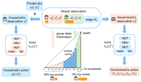
Figure 2: The Markov game between the government and household agents. In the center of the figure, we display the Lorenz curves of households’ wealth distribution. The global observation consists of the average assets $\bar{a}_{t}$, income $\bar{i}_{t}$, and productivity level $\bar{e}_{t}$ of the 50% poorest households and 10% richest households, along with the wage rate $W_{t}$. For the government agent, it observes the global observation and takes tax and spending actions $\{\tau_{t},\xi_{t},\tau_{a,t},\xi_{a,t},r^{G}_{t}\}$ through the actor network. For household agents, they observe both global and private observation, including personal assets $\{a^{i}_{t}\}$ and productivity level $\{e^{i}_{t}\}$, and generate savings and workings actions $\{p^{i}_{t},h^{i}_{t}\}$ through the actor network. The actor network structure in the figure is just an example.

In this section, we model the above problem of optimizing tax policies for the government and developing saving and working strategies for households as multiplayer general-sum Partially Observable Markov Games (POMGs). In the POMGs $\left\langle\mathcal{N},\mathcal{S},\mathcal{O},\mathcal{A},P,\mathcal{R},\gamma\right\rangle$. $\mathcal{N}=\{2,...,N\}$ denotes the set of all agents, $\mathcal{S}$ represents the state space, $\mathcal{O}^{i}$ denotes the observation space for agent $i$, and $\mathcal{O}:=\mathcal{O}^{1}\times...\times\mathcal{O}^{\mathbf{N}}$. $\mathcal{A}^{i}$ signifies the action space for agent $i$, and $\mathcal{A}:=\mathcal{A}^{1}\times...\times\mathcal{A}^{\mathbf{N}}$. $P:\mathcal{S}\times\mathcal{A}\rightarrow\Omega(\mathcal{S})$ denotes the transition probability from state $s\in\mathcal{S}$ to next state $s^{\prime}\in\mathcal{S}$ for any joint action $a\in\mathcal{A}$ over the state space $\Omega(\mathcal{S})$. The reward function $\mathcal{R}:=\{R^{i}\}_{i\in\mathcal{N}}$, here $R^{i}:\mathcal{S}\times\mathcal{A}\times\mathcal{S}\rightarrow\mathbb{R}$ denotes the reward function of the agent $i$ for a transition from $(s,{a})$ to $s^{\prime}$. The discount factor $\gamma\in[0,1)$ keeps constant across time. The specific details of POMGs is shown in the Figure 2 and following paragraphs.

Observation Space $\mathcal{O}$

In the real world, households can observe their own asset $a_{t}$ and productivity ability $e_{t}$, and acquire statistical data about the population from the news. While the government can collect data from all households and access current market prices $W_{t}$. However, the presence of a large number of heterogeneous households results in a considerably high-dimensional state space. To mitigate the dimensionality challenge, TaxAI categorizes households based on their wealth into two groups [82]: the top 10% richest and the bottom 50% poorest households. The average wealth $\{\bar{a}^{r}_{t},\bar{a}^{p}_{t}\}$, income $\{\bar{i}^{r}_{t},\bar{i}^{p}_{t}\}$, and labor productivity levels $\{\bar{e}^{r}_{t},\bar{e}^{p}_{t}\}$ of these two groups are incorporated into the global observation. Therefore, the government’s observation space $\mathcal{O}_{g}=\{W_{t},\bar{a}^{r}_{t},\bar{i}^{r}_{t},\bar{e}^{r}_{t},\bar{a}^{p}_{t},\bar{i}^{p}_{t},\bar{e}^{p}_{t}\}$, while the household agent $i$ can observe the global and its private information $\mathcal{O}_{h}^{i}=\{W_{t},\bar{a}^{r}_{t},\bar{i}^{r}_{t},\bar{e}^{r}_{t},\bar{a}^{p}_{t},\bar{i}^{p}_{t},\bar{e}^{p}_{t},a_{t}^{i},e_{t}^{i}\},i\in\{1,...,N\}$. Moreover, the initialization of state information is calibrated by statistical data from the 2013 Survey of Consumer Finances (SCF) .

Action Space $\mathcal{A}$

The decision-making of household and government agents needs to adhere to budget constraints at every step; however, the abundance of constraints often renders many MARL algorithms ineffective. Therefore, we have introduced proportional actions to alleviate these constraints. For household agents, the optimization of savings $a_{t+1}$ and consumption $c_{t}$ has been transformed into optimizing savings ratio $p_{t}\in(0,1)$ and working time $h_{t}\in[0,1]\cdot h_{max}$, where $h_{max}$ is calibrated by the real wealth-to-income ratio data.

$$p_{t}=\frac{a_{t+1}}{i_{t}-T(i_{t})+a_{t}-T^{a}(a_{t})}$$ (14)

For the government agent, the fiscal policy tools include optimizing tax parameters $\{\tau_{t},\xi_{t},\tau_{a,t},\xi_{a,t}\}$, and the ratio of government spending to GDP $r^{G}_{t}=G_{t}/Y_{t}$. Thus, the action space of the government $\mathcal{A}_{g}$ is $\{\tau_{t},\xi_{t},\tau_{a,t},\xi_{a,t},r^{G}_{t}\}$, while the action space of each household $\mathcal{A}_{h}^{i}$ is $\{p^{i}_{t},h^{i}_{t}\}$.

Reward function $\mathcal{R}$

In TaxAI, each household seeks to maximize their own lifetime utility.

$$r_{h,t}(s_{t},a^{i}_{h,t})=\frac{{c_{t}^{i}}^{1-\theta}}{1-\theta}-\frac{{h_{t}^{i}}^{1+\gamma}}{1+\gamma}$$ (15)

On the other hand, the government’s objectives are more diverse, and we have defined four distinct experimental tasks within TaxAI: (1) Maximizing GDP Growth Rate:

$$r_{g,t}(s_{t},a_{g,t})=\frac{Y_{t}-Y_{t-1}}{Y_{t-1}}$$ (16)

(2) Minimizing Social Inequality:

$$r_{g,t}(s_{t},a_{g,t})=-\text{Gini}(\mathcal{I}_{t})\text{Gini}(\mathcal{W}_{t})$$ (17)

(3) Maximizing Social Welfare:

$$r_{g,t}(s_{t},a_{g,t})=\sum_{i}^{N}\frac{{c_{t}^{i}}^{1-\theta}}{1-\theta}-\frac{{h_{t}^{i}}^{1+\gamma}}{1+\gamma}$$ (18)

(4) Optimizing Multiple Tasks:

$$r_{g,t}(s_{t},a_{g,t})=\frac{Y_{t}-Y_{t-1}}{Y_{t}}-\omega_{1}\cdot\text{Gini}(\mathcal{I}_{t})\text{Gini}(\mathcal{W}_{t})+\omega_{2}\cdot\left(\sum_{i}^{N}\frac{{c_{t}^{i}}^{1-\theta}}{1-\theta}-\frac{{h_{t}^{i}}^{1+\gamma}}{1+\gamma}\right)$$ (19)

In summary, we outline three key improvements made in constructing the TaxAI simulator: Firstly, to bridge the gap between economic models and the real world, we opt to calibrate TaxAI using 2013 SCF data. Secondly, to mitigate the curse of dimensionality associated with high-dimensional state information, we draw inspiration from the World Inequality Report 2022 [82] and employ grouped statistical averages for households as a representation of this high-dimensional state information. Lastly, in response to the abundance of constraints, we introduce the concept of proportional actions, facilitating control over the range of actions to adhere to these constraints. More details about environment setting are shown in Appendix A, including model assumptions, terminal conditions, timing tests B, and parameters.

5 Experiments

This section will begin by introducing 9 baseline algorithms 5.1, followed by conducting the following three sub-experiments: Firstly E.3, we aim to demonstrate the superior performance of MARL algorithms over traditional methods from both macroeconomic and microeconomic perspectives. In the second part 5.3, we conduct an economic analysis of the optimization process for government and heterogeneous household strategies within MARL-based policies. Lastly 5.4, we assess the scalability of TaxAI by comparing the simulation results for different numbers of households, specifically N=10, 100, 1000, and even 10000. Additional results are shown in Appendix E.

5.1 Baselines

We compare 9 different baselines, including traditional economic methods and 4 distinct MARL algorithms, providing a comprehensive MARL benchmark for large-scale heterogeneous multi-agent dynamic games in a tax revenue context. Additional experimental settings are shown in the Appendix E.1.

(1) Traditional Economic Methods: Free Market Policy, Genetic Algorithm (GA) [45].

(2) Independent Learning: Independent PPO [17].

(3) Centralized Training Distributed Execution: MADDPG [62], MAPPO [83], both with parameter sharing.

(4) Heterogeneous-Agent Reinforcement Learning: HAPPO, HATRPO, HAA2C [68].

(5) Mean Field Multi-Agent Reinforcement Learning: Bi-level Mean Field Actor-Critic (BMFAC), shown in Appendix D.

5.2 Comparative Analysis of Multiple Baselines

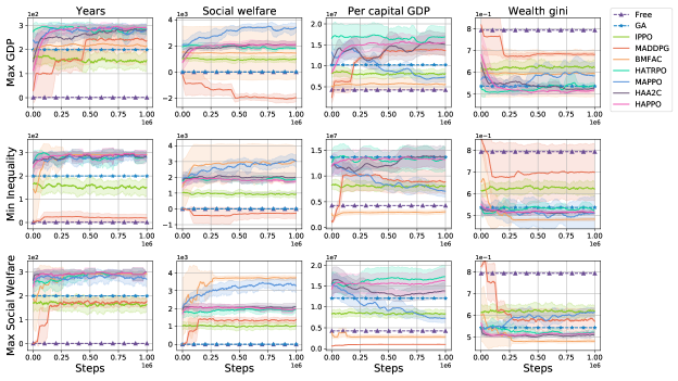
Figure 3: The training curves for 9 baselines on 4 macro-economic indicators under 3 different tasks ($N=100$).

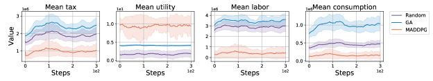
Figure 4: The micro-level behaviors of Random, GA, and MADDPG households while facing identical observations in an episode (300 steps). The subfigure illustrates the average values of labor provided, consumption, taxes paid, and utility for all households at each step. The results reveal that MADDPG households exhibit tax evasion behavior and attain the highest utility.

Table 2: Test results for 9 baselines on 5 economic indicators under maximizing social welfare task with $N=100$ households.

Baselines	Years	Average	Per capital	Wealth	Income
		social welfare	GDP	gini	gini
Free market	$1.00$	$2.92$	$4.25e6$	$0.79$	$\mathbf{0.39}$
GA	$200.00$	$6.85$	$1.21e7$	$0.54$	$0.52$
IPPO	$162.72$	$1035.48$	$8.39e6$	$0.62$	${0.44}$
MADDPG	$204.20$	$1344.63$	$1.02e6$	$0.61$	$0.58$
MAPPO	$274.47$	$3334.71$	$7.28e6$	$0.61$	$0.65$
HAPPO	$298.71$	$1985.97$	$1.63e7$	$0.52$	$0.54$
HATRPO	$\mathbf{300.00}$	$1944.96$	$\mathbf{1.73e7}$	$0.52$	$0.54$
HAA2C	$\mathbf{300.00}$	$2113.31$	$1.39e7$	$0.51$	$0.53$
BMFAC	$292.75$	$\mathbf{3722.20}$	$2.83e6$	$\mathbf{0.48}$	$0.50$

We benchmark 9 baselines on 4 distinct tasks, with the training curves of macroeconomic indicators in 3 tasks shown in Figure 3 and test results shown in Table 2 (Figure 8 in Appendix E presents the training curves for 6 macro-indicators in 4 tasks). In Figure 3, each row represents a task, including maximizing GDP, minimizing inequality, and maximizing social welfare. Each column represents a macroeconomic indicator, where longer years indicate longer economic stability, higher GDP represents a higher level of economic development, and a lower wealth Gini coefficient indicates fairer wealth distribution. The horizontal axis of each subplot represents training steps.

Macroeconomic Perspectives

From Figure 3, it can be observed that in each macro-indicator, most MARL algorithms outperform traditional economic methods. In the GDP optimization task, HATRPO achieves the highest per capita GDP, while BMFAC performs best in the tasks of minimizing inequality and maximizing social welfare. Different algorithms also differ in terms of convergence solutions. MADDPG excels in optimizing GDP but at the cost of reducing social welfare for higher GDP. The BMFAC algorithm excels in optimizing social welfare and the Gini coefficient. HARL algorithms, including HAPPO, HATRPO, and HAA2C, can simultaneously optimize all four macroeconomic indicators, but while achieving the highest GDP, social welfare is not maximized. On the other hand, MAPPO excels in optimizing social welfare.

Microeconomic Perspectives

During the testing phase, we conduct experiments on households following random, GA, and MADDPG policies within the same environment at each step. We utilize 10 distinct random seeds to simulate an economic society spanning 300 timesteps. In Figure 4, these subplots present various microeconomic indicators, including the average tax revenue, average utility, average labor supply, and average consumption for all households at each time step. The random policy represents a strategy unaffected by government tax policies, while the GA policy represents a conventional economics approach. We observe that households under the MADDPG strategy pay the lowest taxes, indicating tax evasion behavior, while simultaneously achieving utility levels significantly surpassing those of the GA and random policies. Labor supply and consumption are statistical measures of household microbehavior. We find that households following the MADDPG strategy tend to opt for low consumption and reduce labor supply strategies.

5.3 Economic Analysis of MARL Policy

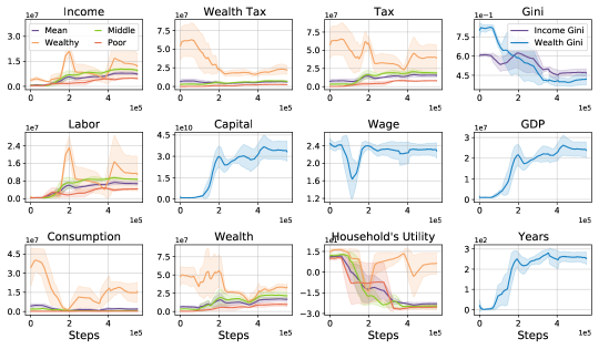
Figure 5: Temporal evolution of economic indicators during MADDPG training on TaxAI ($N=100$).

Table 3: The per capita economic indicators of the MADDPG algorithm during the testing phase at $N=100$ for 3 household groups and the average level across all households.

Households’ groups	Income	Wealth	Total	Labor	Consumption	Wealth	Income	Per year
	tax	tax	tax	supply				utility
The wealthy	$1.9e6$	$\mathbf{1.0e7}$	$\mathbf{1.2e7}$	$2.3e6$	$\mathbf{4.4e7}$	$\mathbf{5.3e7}$	$5.5e6$	$\mathbf{8.7}$
The middle class	$\mathbf{5.7e6}$	$3.0e6$	$8.7e6$	$\mathbf{7.1e6}$	$6.4e5$	$2.1e7$	$\mathbf{7.2e6}$	$-24.1$
The poor	$2.8e6$	$1.2e6$	$4.0e6$	$4.9e6$	$2.3e5$	$9.2e6$	$4.6e6$	$-25.6$
Mean value	$3.8e6$	$2.9e6$	$6.7e6$	$5.5e6$	$4.8e6$	$1.8e7$	$5.7e6$	$-22.7$

The Figure 5 illustrates the training curves of the MADDPG algorithm, aiming to maximize GDP on TaxAI. We utilize the experimental results to analyze the coordination of government actions (tax) and households’ actions (labor and consumption) and their impact on economic indicators. The X-axis represents steps, while the Y-axis represents various economic indicators. In the subplots for income tax, wealth tax, total tax, labor, consumption, and households’ utility, we categorize households into three groups based on wealth: the wealthy (top 10% richest), the middle class (top 10-50% richest), and the poor (50-100% top richest). We display the average indicators for these three groups as well as the average for all households (purple line), other subplots represent macroeconomic indicators (blue line). In each subplot, the solid line represents the mean of experimental results under different seeds, and the shaded area represents the standard deviation. The results of the testing phase are presented in Table 3. The following are two intriguing findings:

1. MADDPG converges towards the highest GDP while compromising social welfare when maximize GDP.

As observed from the Figure 5, during the initial $2e5$ steps, the government increases income and wealth tax, leading to a reduction in the income and wealth Gini, making the wealth distribution more equitable. Social equity is a prerequisite for increasing the duration of the economic system (measured by years). Simultaneously, households choose to increase labor and reduce consumption, leading to a decrease in their utility. As the total savings of households increase, financial intermediaries can provide more production capital to firms. The additional production labor and capital leads to an increase in output (GDP). The wage rate tends to decrease with an increase in labor and increase with a capital increase, exhibiting a trend of initially decreasing and then increasing.

2. Different wealth groups adopt distinct strategies.

From the experimental curves (Figure 5) and results (Table 3) for the wealthy, the middle class, and poor households, we find the following patterns: During $0\sim 2e5$ steps, the wealthy contribute significantly to taxation. To stabilize their wealth, they increase work hours and reduce consumption, leading to a decline in utility. In the second phase ($2e5\sim 4e5$ steps), the wealthy maximize utility by reducing work hours and significantly increasing consumption, even though their wealth levels decrease. In the third phase ($4e5\sim 6e5$ steps), the wealthy simultaneously increase labor and consumption, resulting in increased wealth while maintaining relatively stable utility. On the other hand, the middle class and the poor slightly increase work hours and reduce consumption during all three phases, leading to modest growth in wealth but significantly lower utility compared to the wealthy.

5.4 Scalability of Environment

To demonstrate the scalability of TaxAI in simulating large-scale household agents, we conduct tests with varying numbers of households: 10, 100, 1000, and even 10,000 (as shown in Table 4). The table presents per capita GDP for each baseline, represented as mean ± standard deviation. The results in Table 4 indicate that IPPO and the improved MADDPG algorithm successfully achieve the maximum GDP when $N$ = 10,000, whereas traditional methods yield NA (not available). HATRPO achieves optimal strategies at $N$ = 100 and $N$ = 1000, respectively, while GA only achieves optimal GDP when $N$ is small. The above results indicate that TaxAI is capable of simulating 10,000 household agents, surpassing other benchmarks by a significant margin. Moreover, MARL algorithms can successfully solve the optimal tax problem in large-scale agent scenarios. These two advantages are crucial for simulating real-world society.

Table 4: The per capita GDP achieved by various baselines for different numbers $N$ of households. The maximum GDP values for each $N$ are bolded.

Algorithm	$N$=10	$N$=100	$N$=1000	$N$=10000
Free Market	$1.3e6$	$4.3e6$	$3.9e6$	$4.0e6$
GA	$\mathbf{1.7e8}$	$1.5e7$	NA	NA
IPPO	$5.0e6$	${1.6e7}$	$1.7e7$	$1.6e7$
MADDPG	$3.2e6$	$1.1e7$	${1.7e7}$	$\mathbf{1.7e7}$
MAPPO	$6.1e6$	$7.3e6$	${1.2e7}$	NA
HAPPO	$1.8e7$	$1.6e7$	${1.5e7}$	NA
HATRPO	$3.2e7$	$\mathbf{1.7e7}$	$\mathbf{2.0e7}$	NA
HAA2C	$1.6e7$	$1.4e7$	${1.6e7}$	NA
BMFAC	$4.0e6$	$1.2e7$	$1.2e7$	NA

6 Conclusion

We introduce TaxAI, a large-scale agent-based dynamic economic environment, and benchmark 2 traditional economic methods and 7 MARL algorithms on it. TaxAI, in contrast to prior work, excels in modeling large-scale heterogeneous households, a wider range of economic activities, and tax types. Moreover, it is calibrated using real data and comes with open-sourced simulation code and MARL benchmark. Our results demonstrate the feasibility and superiority of MARL in addressing the optimal taxation problem, while also revealing MARL households’ tax evasion behavior.

In the future, we aim to expand and enrich the economic theory of TaxAI by incorporating a broader range of social roles and strategies. Furthermore, we will enhance the scalability of our simulator to accommodate one billion agents, enabling simulations that closely resemble real-world scenarios. By doing so, we aim to attract more researchers to explore complex economic problems using AI or RL techniques, thereby offering practical and feasible recommendations for social planners and the population.

Appendix A Environment Setting

A.1 Assumption

We have summarized the assumptions involved in the economic model section 3 as follows:

1. Social roles, such as households and government, are considered rational agents.

2. Households are not allowed to incur debt and engage only in risk-free investments.

3. The labor productivity of households is categorized into two states: normal state and super-star state. The dynamic changes in each state follow an AR(1) process.

4. The capital market, goods market, and labor market clear.

5. The technology firm represents all enterprises and factories, producing a homogeneous good, and follows the Cobb-Douglas production function.

6. The financial Intermediary operates without arbitrage.

A.2 Model Dynamics

Figure 6: Illustration of tax impact on the rich and poor households.

Table 5: Variables in Economic Model

Variable	Meaning
$W_{t}$	Wage rate
$e_{t}$	Individual labor productivity levels
$h_{t}$	Working hours
$a_{t}$	Household’s asset(wealth)
$a_{0}$	Household’s initial asset(wealth)
$r_{t}$	interest rate
$i_{t}$	Household’s income
$N$	Households’ number
$\rho_{e}$	Persistence
$u_{t}$	Standard normal shocks
$\sigma_{e}$	Volatility of the standard normal shocks
$\bar{e}$	Labor market ability of super-star state
$p$	Transition probability from normal state
	to super-star state
$q$	Transition probability of remaining
	in super-star state
$\beta$	Discount factor
$\theta$	Coefficient of relative risk aversion (CRRA)
$\gamma$	Inverse Frisch elasticity
$\tau_{s}$	Consumption taxes
$T(i_{t})$	Income taxes
$T^{a}(a_{t})$	Asset taxes
$\tau,\tau_{a}$	Average level of marginal income
	and asset tax
$\xi,\xi_{a}$	Slope of marginal income
	and asset tax schedule
$Y_{t}$	Firm’s output
$K_{t}$	Capital for production
$L_{t}$	Labor for production
$\alpha$	Capital elasticity
$C_{t}$	Households’ gross consumption
$G_{t}$	Government spending
$X_{t}$	Physical capital investment
$\delta$	Depreciation rate
$R_{t}$	Borrowing rate of firm
$G_{t}$	Government spending
$T_{t}$	Households’ gross taxation
$B_{t}$	Debt
$\mathcal{I}_{t}$	Households’ gross post-tax income
$\mathcal{W}_{t}$	Households’ gross post-tax assets
$A_{t}$	Households’ gross deposits
$\omega_{1}$, $\omega_{2}$	Relative weight of social equality and social welfare

To elucidate the dynamics of the economic model more lucidly, we present in Figure 6 the impact of tax changes (from time $t$ to time $t+1$) on individuals with varying levels of wealth. The pie chart in the figure illustrates the current households’ income and wealth distributions, along with the taxation proportions. The green sector represents income or wealth taxation, the blue sector signifies post-tax income, and the pink sector represents post-tax wealth. Furthermore, we calculate the Gini coefficients for income and wealth distributions to demonstrate the effects of changes in tax policies on social equity. (Given that this economic model involves only two households, the Gini coefficients are much smaller than those found in real-world scenarios; therefore, their use here is only for illustrating Gini coefficient variations). Suppose the economy consists of two categories of households—a wealthy household (with initial wealth $a_{t}^{1}=1000$) and a poor household (with initial wealth $a_{t}^{2}=100$). Their income predominantly originates from labor income $W_{t}e_{t}h_{t}$ and asset returns $r_{t-1}a_{t}$ (where $r_{t-1}=0.04$). And they have the same consumption level of $c^{1}_{t}=c^{2}_{t}=30$ for each step.

At step $t$, the wealthy household’s income is $i_{t}^{1}=50+0.04*1000=90$, while the poor household’s income is $i_{t}^{2}=100+0.04*100=104$. Considering tax rate parameters of $\tau=0.2$ and $\xi=\tau_{a}=\xi_{a}=0$, both the wealthy and poor households face an income tax rate of $20\%$, with no taxation on assets. Consequently, the income tax for the wealthy household amounts to $90*0.2=18$, resulting in a post-tax income of $90-18=72$. Similarly, the income tax for the poor household is $20.8$, resulting in a post-tax income of $83.2$. Through the budget constraint, we determine the next-step wealth as $a_{t+1}^{1}=1040.1$ and $a_{t+1}^{2}=151.2$. The Gini coefficient for income is 0.036, while the Gini coefficient for wealth is $0.373$, reflecting the wealth distribution between these two economic agents.

Moving to step $t+1$, despite maintaining unchanged consumption levels and labor incomes for both wealthy and poor households, the increase in wealth fosters an increment in asset returns. Consequently, the incomes for the wealthy and poor households have risen relative to step $t$; namely, $i_{t+1}^{1}=91.6$ and $i_{t+1}^{2}=106.0$. At this juncture, while the tax rate parameter $\tau$ remains unchanged, $\xi$ has been elevated to $0.05$, transforming the income tax function into a non-linear structure and raising tax rates. Meanwhile, the asset tax parameters $\tau_{a}=0.5$ and $\xi_{a}=0.05$ prompt the government to initiate asset taxation. Under equivalent labor income conditions, the wealthy household’s income tax has risen to $30.1$ via Equation 20, while asset taxation has surged to $653.3$. A similar scenario ensues for the poor household. Thus, due to the escalated tax rate, more than half of the asset for both wealthy and poor households is allocated toward taxation. Ultimately, the remaining wealth is $a_{t+2}^{1}=416.4$ and $a_{t+2}^{2}=100.7$. While initially, the wealthy household’s asset was tenfold that of the poor household, the introduction of wealth taxation by the government has reduced this disparity to roughly a fourfold difference. The increase in $\xi$ has led to a marginal decline in the income Gini coefficient, while the wealth tax has significantly lowered the wealth Gini coefficient, concurrently promoting social equity.

$$T\left(i_{t}\right)=i_{t}-(1-\tau)\frac{i_{t}^{1-\xi}}{1-\xi},\quad T^{a}\left(a_{t}\right)=a_{t}-\frac{1-\tau_{a}}{1-\xi_{a}}a_{t}^{1-\xi_{a}}$$ (20)

A.3 Environment Parameters

The assigned parameters of TaxAI are shown in table 6. At the beginning of each episode, we initialize households’ assets $\{a^{i}_{0}\}^{N}_{i}$ via the statistical data from the 2013 Survey of Consumer Finances (SCF) data and calibrate aggregate labors $L_{t}$ and the maximum of working hours $h_{max}$ based on the wealth-to-income ratio computed from the SCF data.

Table 6: Assigned Parameters in Environment

Hyperparameter	Value
CRRA $\theta$	1
Inverse Frisch elasticity $\gamma$	2
discount factor $\beta$	0.975
capital elasticity $\alpha$	$1/3$
depreciation rate $\delta$	$0.06$
return to savings $r_{t}$	0.04
consumption tax rate $\tau_{s}$	0.065
normal to super-star probability $p$	$2.2e^{-6}$
remain in super-star probability $q$	0.990
persistence $\rho_{e}$	0.982
volatility of the standard normal shocks $\sigma_{e}$	0.200
super ability times $\bar{e}$	504.3
Wealth to income ratio	6.6

A.4 Teriminal Condition

We will terminate the current episode under the following circumstances:

• If the maximum number of steps in an episode is reached.

• If the Gini coefficient of income or wealth exceeds a threshold;

• If the Gross Domestic Product (GDP) is insufficient to cover the total consumption of households ($C_{t}+G_{t}>Y_{t}$).

• In the event of household bankruptcy ($a_{t}^{i}<0$).

• If the calculation of households’ or government’s rewards results in an overflow or leads to the appearance of NaN (Not-a-Number) values.

A.5 Reinforcement learning API

Installation Our open-source TaxAI simulator is available at https://github.com/jidiai/TaxAI/. We recommend that users set up a virtual environment to manage the project’s packages and dependencies, and then clone the code repository using git for package installation as shown below:

⬇

1$ conda create -n TaxAI python=3.6

2$ conda activate TaxAI

3$ git clone https://github.com/jidiai/TaxAI.git

4$ cd TaxAI

5$ pip install -r requirements.txt

Start an episode Here is an example code on TaxAI GDP task, assuming that both the government agent and household agents employ a random policy.

⬇

1from env.env_core import economic_society

2from omegaconf import OmegaConf

3

4yaml_cfg = OmegaConf.load(f’./cfg/default.yaml’) # get environment parameters

5env = economic_society(yaml_cfg.Environment)

6# get the action max

7gov_action_max = env.government.action_space.high[0]

8house_action_max = env.households.action_space.high[0]

9global_obs, private_obs = env.reset()

10for _ in range(100):

11 gov_action = env.government.action_space.sample()

12 house_action = env.households.action_space.sample()

13 # gov_action & house_action is in (-1,+1)

14 action = {env.government.name: gov_action * gov_action_max,

15 env.households.name: house_action * house_action_max}

16 next_global_obs, next_private_obs, gov_reward, house_reward, done = env.step(action)

17 print("gov␣reward:", gov_reward, "---␣households␣reward:", house_reward)

18 if done:

19 global_obs, private_obs = env.reset()

20env.close()

If users obtain a similar output as follows, it indicates a successful installation of the TaxAI simulator.

⬇

1gov reward: 8.41615569709358

2households reward: [[-12.25838861]

3 [ 13.63084777]

4 [ 8.35009887]

5 [ 11.44650562]

6 [-15.38658803]

7 [ 11.56392558]

8 [-24.6209271 ]

9 [ 11.79586767]

10 [-23.43364898]

11 [ 12.78705537]]

12......

Appendix B Timing Tests

Table 7 shows the number of dynamics evaluations per second in a single thread. Results are averaged over 10 episodes on AMD EPYC 7742 64-Core Processor with GPU GA100 [GRID A100 PCIe 40GB].

Table 7: The number of dynamics evaluations per second in a single thread.

Algorithm	$N$=10	$N$=100	$N$=1000	$N$=10000
Number of steps	$1799.927$	$482.335$	$46.983$	$4.018$
num of episodes	$6.289$	$1.689$	$0.157$	$0.013$
episode length	$285.900$	$285.400$	$300.000$	$300.000$

Appendix C Genetic Algorithm

In this subsection, we provide additional details regarding the implementation of genetic algorithms. To evaluate the performance of different policies, we employ relevant economic indicators such as GDP and the Gini coefficient as the fitness function. Our genetic algorithm implementation includes the utilization of uniform crossover and simple mutation. The specific parameters used in the algorithm are presented in Table 11.

For household agents, we refer to Heathcote’s [84] approach in selecting saving and working hours for households under the shocks of agent productivity and preferences. However, our model does not incorporate the preference for working and consumption, denoted as $\varphi_{t}=0$. The productivity of work is determined by

$$\log e_{t}=\alpha_{t}+\varepsilon_{t}$$ (21)

$$\alpha_{t}=\alpha_{t-1}+\omega_{t}$$ (22)

$$\varepsilon_{t}=\kappa_{t}+\theta_{t}$$ (23)

The households strategies are obtained by competitive equilibrium under the productivity shock. The proportions of consumption to income and working hours $c_{t}^{a}$ and $h_{t}^{a}$ are calculated using the following equations:

$$\log c_{t}^{a}\left(s^{t}\right)=-\varphi_{t}+\frac{1+\gamma}{\gamma+\theta}\alpha_{t}+\mathcal{M}_{t}^{a}$$ (24)

$$\log h_{t}^{a}\left(s^{t}\right)=-\varphi_{t}+\frac{1-\theta}{\gamma+\theta}\alpha_{t}+\frac{1}{\gamma}\left(\kappa_{t}+\theta_{t}\right)-\frac{\theta}{\gamma}\mathcal{M}_{t}^{a}$$ (25)

$$\mathcal{M}_{t}^{a}=\gamma/(\gamma+\theta)\log\left(\int\exp\left(\frac{1+\gamma}{\gamma}\theta_{t}\right)dF_{\theta t}\right)$$ (26)

where $\omega_{t}$ and $\theta_{t}$ is an independently distributed shock, $\kappa_{t}$ is a permanent shock ($\kappa_{t}=0$ in our experiment).

Appendix D Bi-level Mean Field Actor-Critic Algorithm

We propose a Bi-level Mean Field Actor-Critic (BMFAC) algorithm for the Stackelberg game between the government and $N$ households. In our BMFAC method, the government serves as the leader and the households as equal followers. The objective of the government is to maximize its objective by setting tax rates and government spending while anticipating the households’ actions. Conversely, households aim to optimize their lifetime utility by making decisions regarding their saving policies and working hours. Initially, the government’s action is initialized to a free-market policy (without taxes), and we employ an iterative process to optimize the household agents’ policies in the inner loop. Given the household agents’ policies, we generate sample trajectories for the government agent and update its actor and critic networks accordingly. Subsequently, we sample data and update the networks for the households, considering the government’s policy. This iterative process continues until convergence is attained.

Algorithm 1 BMFAC: Bi-level Mean Field Actor Critic

1:  Initialize $Q_{g}^{\phi},Q_{h}^{\phi^{-}},\pi^{\theta}_{g},\pi^{\theta_{-}}_{h}$, and $\bar{a}_{h}^{i}$ for all $i\in\{1,\ldots,N\}$

2:  Initialize the government policy as the free market rules $a_{g}^{0}=\{0,0,0,0,0.189\}$.

3:  for Outer Loop do

4:     for Inner Loop do

5:        for each sample step do

6:           Given the government policy $\pi_{g}$, the government agent sample action $a_{g}\sim\pi_{g}(o_{g})$; the household agent $i$ sample action $a^{i}_{h}\sim\pi_{h}({o_{h}^{i}},a_{g})$.

7:           Take the actions and observe $r_{g},\mathbf{r_{h}}=\{r_{h}^{1},...,r_{h}^{N}\}$ and next state $o_{g}^{\prime},\mathbf{o_{h}}=\{{o_{h}^{1}}^{\prime},...,{o_{h}^{N}}^{\prime}\}$.

8:           Store $\left\langle o_{g},\mathbf{o_{h}},a_{g},\mathbf{a_{h}},r_{g},\mathbf{r_{h}},o^{\prime}_{g},\mathbf{o_{h}}^{\prime}\right\rangle$ in replay buffer $\mathscr{D}$.

9:        end for

10:        Update the households’ actor and critic for $N^{h}_{\text{update}}$ steps:

$$\psi\leftarrow\psi-\lambda_{Q}\hat{\nabla}_{\psi}\mathscr{L}(\psi)$$

$$\psi^{-}\leftarrow\psi^{-}-\lambda_{Q}\hat{\nabla}_{\psi^{-}}\mathscr{L}(\psi^{-})$$

$$\sigma\leftarrow\sigma-\lambda_{\pi}\hat{\nabla}_{\sigma}\mathscr{L}(\sigma)$$

11:     end for

12:     for each sample step do

13:        Given the households policy $\pi_{h}$, the government agent sample action $a_{g}\sim\pi_{g}(o_{g})$; the household agent $i$ sample action $a^{i}_{h}\sim\pi_{h}({o_{h}^{i}},a_{g})$.

14:        Take the actions and observe $r_{g},\mathbf{r_{h}}=\{r_{h}^{1},...,r_{h}^{N}\}$ and next state $o_{g}^{\prime},\mathbf{o_{h}}=\{{o_{h}^{1}}^{\prime},...,{o_{h}^{N}}^{\prime}\}$.

15:        Store $\left\langle o_{g},\mathbf{o_{h}},a_{g},\mathbf{a_{h}},r_{g},\mathbf{r_{h}},o^{\prime}_{g},\mathbf{o_{h}}^{\prime}\right\rangle$ in replay buffer $\mathscr{D}$.

16:     end for

17:     Update the government’s actor and critic for $N^{g}_{\text{update}}$ steps:

$$\phi\leftarrow\phi-\lambda_{Q}\hat{\nabla}_{\phi}\mathscr{L}(\phi)$$

$$\phi^{-}\leftarrow\phi^{-}-\lambda_{Q}\hat{\nabla}_{\phi^{-}}\mathscr{L}(\phi^{-})$$

$$\theta\leftarrow\theta-\lambda_{\pi}\hat{\nabla}_{\theta}\mathscr{L}(\theta)$$

18:  end for

D.1 Government Agent

We update the government agent via the actor-critic method. We consider double Q-function $Q_{\phi}(\mathbf{o}_{t},\mathbf{a}_{t})$, $Q_{\phi^{-}}(\mathbf{o}_{t},\mathbf{a}_{t})$, and a policy $\pi_{\theta}(a_{g,t}\mid o_{g,t})$. For example, the value functions can be modeled as expressive neural networks and the policy as a Gaussian with mean and covariance given by neural networks. We will next derive update rules for these parameter vectors.

The critic network

The Q-function parameters can be trained to minimize the soft Bellman residual.

$$\mathscr{L}\left(\phi\right)=\left(y_{g}-Q_{\phi}\left(o_{g},a_{g},\{\pi_{h}(o_{h}^{i},a_{g})\}_{i}^{N}\right)\right)^{2}$$ (27)

where the target mean field value with the weight $\phi^{-}$ is computed by

$$y_{g}=r_{g}+\gamma\mathbb{E}_{a^{\prime}_{g}\sim\pi_{g}}Q_{\phi^{-}}(s^{\prime}_{g},a^{\prime}_{g},\{\pi_{h}(o_{g}^{\prime},{o_{h}^{i}}^{\prime},a_{g}^{\prime})\}_{i}^{N})$$ (28)

Differentiating $\mathscr{L}\left(\phi\right)$ gives

$$\nabla_{\phi}\mathscr{L}\left(\phi\right)=\left(y_{g}-Q_{\phi}\left(o_{g},a_{g},\{\pi_{h}(o_{h}^{i},a_{g})\}_{i}^{N}\right)\right)$$ (29)

$$\nabla_{\phi}Q_{\phi}\left(o_{g},a_{g},\{\pi_{h}(o_{h}^{i},a_{g})\}_{i}^{N}\right)$$

which enables the gradient-based optimizers for training.

The actor network

The policy network of the government $\pi^{\theta}_{g}$ is training by the sampled policy gradient:

$$\nabla_{\theta}\mathscr{L}\left(\theta\right)\approx\nabla_{\theta}\log{\pi_{g}^{\theta}(o_{g})}Q_{\phi}\left(o_{g},a_{g},\{\pi_{h}(o_{h}^{i},a_{g})\}_{i}^{N}\right)$$ (30)

D.2 Household Agents

We update household agents via the mean field actor-critic method. We consider double Q-function $Q_{\psi}(\mathbf{o}_{t},\mathbf{a}_{t})$, $Q_{\psi^{-}}(\mathbf{o}_{t},\mathbf{a}_{t})$ as a shared critic and a shared policy $\pi_{\sigma}(a_{h,t}\mid o_{h,t})$ for all household agents. For example, the value functions can be modeled as expressive neural networks and the policy as a Gaussian with mean and covariance given by neural networks. We will next derive update rules for these parameter vectors.

The critic network

The Q-function parameters can be trained to minimize the Bellman residual.

$$\mathscr{L}\left(\phi\right)=\left(y_{h}-Q_{\psi}\left(o_{h},a_{g},a_{h},\bar{A}_{h}\right)\right)^{2}$$ (31)

with

$$y=r_{h}+\gamma V_{\psi^{-}}^{\mathrm{MF}}\left(o_{h}^{\prime}\right)$$ (32)

The mean field value function $V^{MF}(o^{\prime}_{h})$ for household agent $i$ over the government’s action $a_{g}$ is

$$V^{MF}_{\psi^{-}}\left(o^{\prime}_{h}\right)=\mathbb{E}_{a^{\prime}_{h},\bar{A}^{\prime}_{h}\sim\pi_{h}(o^{\prime}_{h})}Q(o^{\prime}_{h},a^{\prime}_{g},a^{\prime}_{h},\bar{A}_{h}^{\prime})$$ (33)

The mean action $\bar{a}_{h}^{i}$ of all $i$’s neighbors is first calculated by averaging the actions $a^{j}$ taken by $i$’s $N^{i}$ neighbors from policies $\pi_{t}(o_{h}^{j})$ parametrized by their previous mean actions $\bar{a}^{j}_{-}$

$$\bar{a}^{i}=\frac{1}{N^{i}}\sum_{j}a^{j},a^{j}\sim\pi_{t}\left(\cdot\mid o_{h}^{j},\bar{a}_{-}^{j}\right)$$ (34)

The gradient of the households’ critic network is given by

$$\nabla_{\psi}\mathscr{L}\left(\phi\right)=\left(y_{h}-Q_{\psi}\left(o_{h},a_{g},a_{h},\bar{A}_{h}\right)\right)\nabla_{\psi}Q_{\psi}\left(o_{h},a_{g},a_{h},\bar{A}_{h}\right)$$ (35)

The actor network

With each $\bar{a}^{i}$ calculated as in Eq. 34, the policy network of household agents $\pi^{\sigma}_{h}$, i.e. the actor, of MF-AC is trained by the sampled policy gradient:

$$\nabla_{\sigma}\mathscr{L}\left(\sigma\right)\approx\log\pi_{\sigma}(o_{h},\bar{A}_{h})Q_{\psi}\left(o_{h},a_{g},a_{h},\bar{A}_{h}\right)$$ (36)

Appendix E Additional Results

E.1 Baselines Setting

(1) Free Market Policy The government takes a hands-off approach to market activities, and households choose to work and saving actions stochastically.

(2) Genetic Algorithm The government employs the genetic algorithm to optimize tax policies, while household agents adopt consumption and labor supply strategies following Heathcote’s work [84]. See Appendix C for more details.

(3) Independent PPO Both the government and households utilize the PPO policy, treat other agents as part of the environment and learn policies based on local observations.

(4) Multi-Agent Deep Deterministic Policy Gradient (MADDPG) To address large-scale multi-agent problems using MADDPG, we categorize the agents into 4 groups: the government, the top 10% richest households, the top 10-50% richest households, and the bottom 50% richest households. Each group of agents shares an actor and a centralized critic and updates their networks using the MADDPG method.

(5) Multi-Agent Proximal Policy Optimization (MAPPO) Both government and household agents utilize a PPO actor and adopt a centralized value function. The government agent and household agents share a common actor network, with the observation and action spaces of heterogeneous agents aligned.

(6) Bi-level Mean Field Actor-Critic (BMFAC) The government acts as the leader agent and updates its policy using the policy gradient method. While the household act as follower agents, sharing a common actor and critic, and updating networks via the mean-field actor-critic approach [65]. The government and households utilize a bi-level optimization approach, iteratively optimizing their policies to converge toward a Markov Perfect Equilibrium. More details are provided in the Appendix D.

(7) Heterogeneous-Agent Reinforcement Learning (HARL) HARL algorithms (HAPPO, HATRPO, HAA2C) employ heterogeneous actors and a joint advantage estimator, without the need for relying on restrictive parameter-sharing trick.

E.2 Training Curves

To demonstrate the learning performance of the MARL algorithms on the TaxAI simulator, we present training curves for 9 baselines across four different tasks (shown in Figure 7). Among these baselines, GA and free-market policy are not learning algorithms, thus their convergence results are represented by straight lines. The MARL algorithms are represented by solid lines indicating the mean values, while the shaded areas reflect the variances of these economic indicators. In the subplots, each row represents an economic indicator, while each column corresponds to the experimental task. From Figure 7, it is evident that the MARL algorithm outperforms the traditional methods on six economic indicators across each task. Different algorithms excel in different tasks. For instance, HATRPO achieves the highest per capita GDP in the maximizing GDP task, while BMFAC achieves the lowest wealth Gini coefficient and the highest social welfare in the tasks of minimizing social inequality and maximizing welfare. In the multi-task scenario, different algorithms prioritize different optimization objectives. These results highlight the effectiveness and superiority of the MARL algorithms in finding optimal tax policies for the government and optimal working and saving strategies for households.

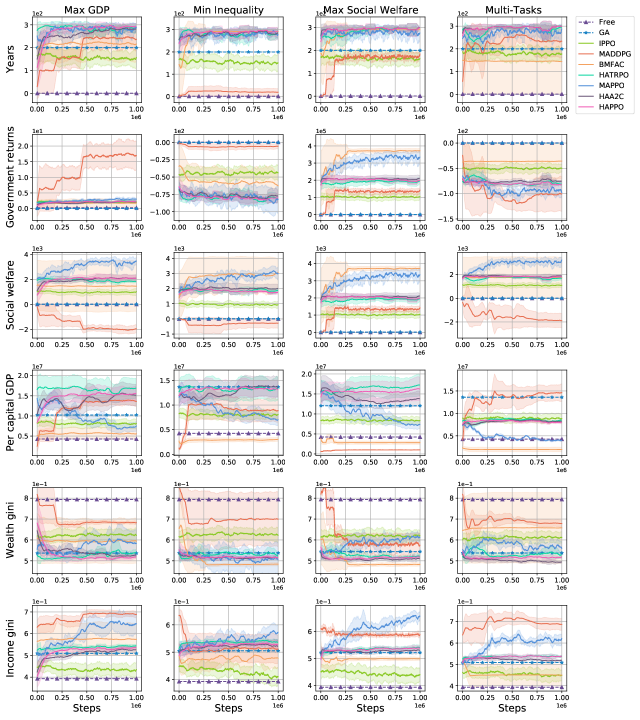
Figure 7: The training curves for 9 baselines on 6 economic indicators in 4 different tasks ($N=100$).

E.3 Economic Evolution

To explore the optimal solution to the dynamic game between the government and households (N=100), we implement five baselines over three tasks: maximizing GDP growth rate, minimizing social inequality, and maximizing social welfare. Additionally, we test the converged policies and demonstrate the macroeconomic indicators, such as per capita GDP, wealth distribution, and social welfare, as the number of steps increases. This analysis aims to illustrate the evolutionary process of the economy under different algorithms.

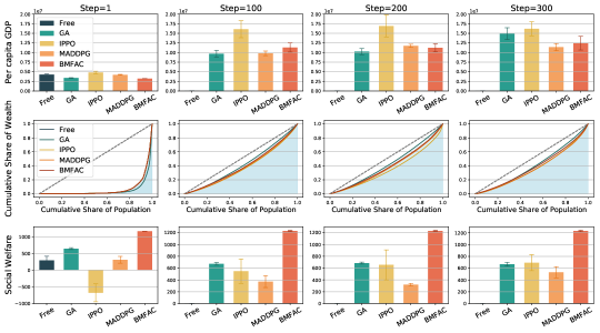
Figure 8: The economic evolution process of different algorithms in the TaxAI environment. Each row represents a macroeconomic indicator, while each column represents a time step in the evolution.

In Figure 8, each row represents a macroeconomic indicator, with the first row corresponding to per capita GDP and the third-row representing social welfare. The horizontal axis represents different baselines and the height of the bars shows the GDP and social welfare at the current step. The second row displays the Lorenz curves for wealth distribution, where the vertical axis represents the cumulative proportion of wealth and the horizontal axis represents the cumulative proportion of a population ranked by their wealth. The five curves correspond to the Lorenz curves of different baselines, where a closer proximity to the line of perfect equality indicates a higher level of equality in wealth distribution. Each column is divided based on steps, where we define each step as representing one year in the real world. The government and households make decisions at each time step. The maximum step is set to 300. When an economy satisfies a terminal condition, such as insufficient production to meet consumer demand or the Gini coefficient of wealth distribution exceeding a threshold, the economic system stops evolving.

The experimental results in Figure 8 provide evidence for the ability of TaxAI to simulate the economic evolution and the feasibility and superiority of MARL algorithms in solving the optimal taxation problem. Firstly, the free market policy struggles to progress beyond 100 steps, whereas the other four tax optimization policies can evolve up to 300 steps, thereby highlighting the efficacy of the proposed policy interventions for ensuring the sustainability of the economy. Furthermore, with the increasing steps, the GDP and social welfare associated with the GA, IPPO, MADDPG, and BMFAC methods continuously increase, while wealth inequality decreases. This alignment with the given optimization objectives reveals the feasibility of these methods in solving the optimal tax problem. Lastly, in the tasks evaluating GDP and social welfare, IPPO achieves the highest GDP, while BMFAC significantly outperforms other algorithms in terms of social welfare. In terms of the Lorenz curve, 5 baselines except the free market policy converge from an unequal state to a relatively higher level of equality. These results demonstrate that MARL methods possess the capability to simulate the evolution of the economy and attain optimal tax policies that surpass those achieved by traditional approaches such as the free market and GA.

The hyperparameters used in baselines algorithms are shown in Table 8, 9, 10.

Table 8: Public Hyperparameters of Baselines Algorithms

Hyperparameter	Value
Discount factor $\gamma$	0.975
Critic learning rate	3e-4
Actor learning rate	3e-4
Replay buffer size	1e6
Init exploration steps	1000
Num of epochs	1500
Epoch length	500
Batch size	128
Tau $\tau$	5e-3
Evaluation epochs	10
Hidden size	128

Table 9: Hyperparameters of IPPO Algorithm

Hyperparameter	Value
Tau $\tau$	0.95
Gamma $\gamma$	0.99
Eps $\epsilon$	1e-5
Clip	0.1
Vloss coef	0.5
Ent coef	0.01
Max grad norm	0.5
Update frequency	1

Table 10: Hyperparameters of MADDPG Algorithm

Hyperparameter	Value
Update frequency	10
Noise rate	0.1
Epsilon	0.1
Save interval	100

Table 11: Hyperparameters of Genetic Algorithm

Hyperparameter	Value
DNA size	12
Pop size	100
Crossover rate	0.8
Mutation rate	0.1
Max generations	200

Table 12: Hyperparameters of MAPPO, HAPPO, HATRPO, HAA2C Algorithm

Hyperparameter	value	Hyperparameter	value	Hyperparameters	Value
Eval episode	20	Optimizer	Adam	Num mini-batch	1
Gamma	0.99	Optim eps	$1\mathrm{e}-5$	Batch size	4000
Gain	0.01	Hidden layer	1	Training threads	20
Std y coef	0.5	Actor network	MLP	Rollout threads	4
Std x coef	1	Max grad norm	10	Episode length	300
Activation	ReLU	Hidden layer dim	64	Critic lr	$5\mathrm{e}-3$
Actor lr	$5\mathrm{e}-5$	Gov actor lr	$5\mathrm{e}-4$	Gov critic lr	$5\mathrm{e}-4$

References

- [1] Adam Smith. The theory of moral sentiments. Penguin, 2010.
- [2] Adam Smith. An Inquiry into the Nature and Causes of the Wealth of Nations. BoD–Books on Demand, 2023.
- [3] Cass R Sunstein. Free markets and social justice. Oxford University Press on Demand, 1997.
- [4] William J Baumol. The free-market innovation machine: Analyzing the growth miracle of capitalism. Princeton university press, 2002.
- [5] John McMillan and Barry Naughton. How to reform a planned economy: lessons from china. Oxford review of economic policy, 8(1):130–143, 1992.
- [6] Mike W Peng and Peggy Sue Heath. The growth of the firm in planned economies in transition: Institutions, organizations, and strategic choice. Academy of management review, 21(2):492–528, 1996.
- [7] Victor Nee. Organizational dynamics of market transition: Hybrid forms, property rights, and mixed economy in china. Administrative science quarterly, pages 1–27, 1992.
- [8] Sanford Ikeda. Dynamics of the mixed economy: Toward a theory of interventionism. Routledge, 2002.
- [9] Norman Johnson. Mixed economies welfare. Routledge, 2014.
- [10] Paul Davidsson. Agent Based Social Simulation: A Computer Science View. 5.
- [11] Eric Bonabeau. Agent-based modeling: Methods and techniques for simulating human systems. 99:7280–7287.
- [12] Xiaochen Li, Wenji Mao, Daniel Zeng, and Fei-Yue Wang. Agent-Based Social Simulation and Modeling in Social Computing. In Intelligence and Security Informatics, pages 401–412. Springer, Berlin, Heidelberg.
- [13] John Geanakoplos, Robert Axtell, Doyne J. Farmer, Peter Howitt, Benjamin Conlee, Jonathan Goldstein, Matthew Hendrey, Nathan M. Palmer, and Chun-Yi Yang. Getting at systemic risk via an agent-based model of the housing market. 102(3):53–58.
- [14] Jakob Foerster, Ioannis Alexandros Assael, Nando De Freitas, and Shimon Whiteson. Learning to communicate with deep multi-agent reinforcement learning. Advances in neural information processing systems, 29, 2016.
- [15] Frans A Oliehoek, Christopher Amato, et al. A concise introduction to decentralized POMDPs, volume 1. Springer, 2016.
- [16] Sainbayar Sukhbaatar, Rob Fergus, et al. Learning multiagent communication with backpropagation. Advances in neural information processing systems, 29, 2016.
- [17] Stephan Zheng, Alexander Trott, Sunil Srinivasa, David C. Parkes, and Richard Socher. The AI Economist: Taxation policy design via two-level deep multiagent reinforcement learning. 8(18):eabk2607.
- [18] Michael Curry, Alexander Trott, Soham Phade, Yu Bai, and Stephan Zheng. Analyzing Micro-Founded General Equilibrium Models with Many Agents using Deep Reinforcement Learning.
- [19] S. Rao Aiyagari. Optimal Capital Income Taxation with Incomplete Markets, Borrowing Constraints, and Constant Discounting. Journal of Political Economy, 103(6):1158–1175, 1995.
- [20] S. R. Aiyagari. Uninsured Idiosyncratic Risk and Aggregate Saving. The Quarterly Journal of Economics, 109(3):659–684, August 1994.
- [21] Adam Smith. The wealth of nations [1776], volume 11937. na, 1937.
- [22] David Gale. The law of supply and demand. Mathematica scandinavica, pages 155–169, 1955.
- [23] Emil Kauder. History of marginal utility theory, volume 2238. Princeton University Press, 2015.
- [24] Robert J Barro. The aggregate-supply/aggregate-demand model. Eastern Economic Journal, 20(1):1–6, 1994.
- [25] Amitava Krishna Dutt and Peter Skott. Keynesian theory and the aggregate-supply/aggregate-demand framework: a defense. Eastern Economic Journal, 22(3):313–331, 1996.
- [26] Amitava Krishna Dutt. Aggregate demand, aggregate supply and economic growth. International review of applied economics, 20(3):319–336, 2006.
- [27] Shelby D Hunt and Robert M Morgan. The comparative advantage theory of competition. Journal of marketing, 59(2):1–15, 1995.
- [28] Arnaud Costinot. An elementary theory of comparative advantage. Econometrica, 77(4):1165–1192, 2009.
- [29] Robert E Lucas. Two illustrations of the quantity theory of money. The American Economic Review, 70(5):1005–1014, 1980.
- [30] Milton Friedman. Quantity theory of money. In Money, pages 1–40. Springer, 1989.
- [31] David Cass. Optimum growth in an aggregative model of capital accumulation. The Review of economic studies, 32(3):233–240, 1965.
- [32] Tjalling C Koopmans. On the concept of optimal economic growth. 1963.
- [33] Peter A Diamond and James A Mirrlees. Optimal taxation and public production i: Production efficiency. The American economic review, 61(1):8–27, 1971.
- [34] Peter A Diamond and James A Mirrlees. Optimal taxation and public production ii: Tax rules. The American Economic Review, 61(3):261–278, 1971.
- [35] Paul A Samuelson. An exact consumption-loan model of interest with or without the social contrivance of money. Journal of political economy, 66(6):467–482, 1958.
- [36] Peter A Diamond. National debt in a neoclassical growth model. The American Economic Review, 55(5):1126–1150, 1965.
- [37] Oded Galor. A two-sector overlapping-generations model: A global characterization of the dynamical system. Econometrica: Journal of the Econometric Society, pages 1351–1386, 1992.
- [38] S Rao Aiyagari. Optimal capital income taxation with incomplete markets, borrowing constraints, and constant discounting. Journal of political Economy, 103(6):1158–1175, 1995.
- [39] Truman Bewley. Stationary monetary equilibrium with a continuum of independently fluctuating consumers. Contributions to mathematical economics in honor of Gérard Debreu, 79, 1986.
- [40] Jess Benhabib and Alberto Bisin. Skewed wealth distributions: Theory and empirics. Journal of Economic Literature, 56(4):1261–91, 2018.
- [41] Varadarajan V Chari and Patrick J Kehoe. Optimal fiscal and monetary policy. Handbook of macroeconomics, 1:1671–1745, 1999.
- [42] Corina Boar and Virgiliu Midrigan. Efficient redistribution. Journal of Monetary Economics, 131:78–91, 2022.
- [43] Ozan Bakış, Barış Kaymak, and Markus Poschke. Transitional dynamics and the optimal progressivity of income redistribution. Review of Economic Dynamics, 18(3):679–693, 2015.
- [44] David Domeij and Jonathan Heathcote. On the distributional effects of reducing capital taxes. International economic review, 45(2):523–554, 2004.
- [45] Sebastian Dyrda, Marcelo Pedroni, et al. Optimal fiscal policy in a model with uninsurable idiosyncratic shocks. In 2016 Meeting Papers, volume 1245, 2016.
- [46] Daniel Carroll, André Victor Doherty Luduvice, and Eric R Young. Optimal fiscal reform with many taxes. 2023.
- [47] David A Love. Optimal rules of thumb for consumption and portfolio choice. The Economic Journal, 123(571):932–961, 2013.
- [48] Jonathan Heathcote, Kjetil Storesletten, and Giovanni L Violante. Optimal tax progressivity: An analytical framework. The Quarterly Journal of Economics, 132(4):1693–1754, 2017.
- [49] Leigh Tesfatsion. Introduction to the special issue on agent-based computational economics. Journal of Economic Dynamics and Control, 25(3-4):281–293, 2001.
- [50] Mitja Steinbacher, Matthias Raddant, Fariba Karimi, Eva Camacho Cuena, Simone Alfarano, Giulia Iori, and Thomas Lux. Advances in the agent-based modeling of economic and social behavior. SN Business & Economics, 1(7):99, 2021.
- [51] Nipa Basu, R Pryor, and Tom Quint. Aspen: A microsimulation model of the economy. Computational Economics, 12:223–241, 1998.
- [52] Giovanni Dosi, Giorgio Fagiolo, Mauro Napoletano, and Andrea Roventini. Income distribution, credit and fiscal policies in an agent-based keynesian model. Journal of Economic Dynamics and Control, 37(8):1598–1625, 2013.
- [53] Tomas B Klos and Bart Nooteboom. Agent-based computational transaction cost economics. Journal of Economic Dynamics and Control, 25(3-4):503–526, 2001.
- [54] Lucian Buşoniu, Robert Babuška, and Bart De Schutter. Multi-agent reinforcement learning: An overview. pages 183–221.
- [55] Kaiqing Zhang, Zhuoran Yang, and Tamer Başar. Multi-agent reinforcement learning: A selective overview of theories and algorithms. pages 321–384.
- [56] Richard S. Sutton and Andrew G. Barto. Reinforcement Learning: An Introduction. MIT press.
- [57] Ming Tan. Multi-agent reinforcement learning: Independent vs. cooperative agents. In Proceedings of the Tenth International Conference on Machine Learning, pages 330–337.
- [58] Pattie Maes and Rodney A Brooks. Learning to coordinate behaviors. In AAAI, volume 90, pages 796–802. Boston, MA, 1990.
- [59] Christian Schroeder de Witt, Tarun Gupta, Denys Makoviichuk, Viktor Makoviychuk, Philip HS Torr, Mingfei Sun, and Shimon Whiteson. Is independent learning all you need in the starcraft multi-agent challenge? arXiv preprint arXiv:2011.09533, 2020.
- [60] Timothy P Lillicrap, Jonathan J Hunt, Alexander Pritzel, Nicolas Heess, Tom Erez, Yuval Tassa, David Silver, and Daan Wierstra. Continuous control with deep reinforcement learning. arXiv preprint arXiv:1509.02971, 2015.
- [61] Ardi Tampuu, Tambet Matiisen, Dorian Kodelja, Ilya Kuzovkin, Kristjan Korjus, Juhan Aru, Jaan Aru, and Raul Vicente. Multiagent Cooperation and Competition with Deep Reinforcement Learning.
- [62] Ryan Lowe, given-i=YI family=WU, given=YI, Aviv Tamar, Jean Harb, OpenAI Pieter Abbeel, and Igor Mordatch. Multi-Agent Actor-Critic for Mixed Cooperative-Competitive Environments. In Advances in Neural Information Processing Systems, volume 30. Curran Associates, Inc.
- [63] Tabish Rashid, Mikayel Samvelyan, Christian Schroeder De Witt, Gregory Farquhar, Jakob Foerster, and Shimon Whiteson. Monotonic value function factorisation for deep multi-agent reinforcement learning. 21(1):7234–7284.
- [64] Chao Yu, Akash Velu, Eugene Vinitsky, Jiaxuan Gao, Yu Wang, Alexandre Bayen, and Yi Wu. The surprising effectiveness of ppo in cooperative multi-agent games. 35:24611–24624.
- [65] Yaodong Yang, Rui Luo, Minne Li, Ming Zhou, Weinan Zhang, and Jun Wang. Mean field multi-agent reinforcement learning. In International Conference on Machine Learning, pages 5571–5580. PMLR.
- [66] Ming Zhou, Yong Chen, Ying Wen, Yaodong Yang, Yufeng Su, Weinan Zhang, Dell Zhang, and Jun Wang. Factorized q-learning for large-scale multi-agent systems. In Proceedings of the First International Conference on Distributed Artificial Intelligence, pages 1–7.
- [67] Haotian Gu, Xin Guo, Xiaoli Wei, and Renyuan Xu. Mean-field multi-agent reinforcement learning: A decentralized network approach.
- [68] Yifan Zhong, Jakub Grudzien Kuba, Siyi Hu, Jiaming Ji, and Yaodong Yang. Heterogeneous-agent reinforcement learning. arXiv preprint arXiv:2304.09870, 2023.
- [69] Rui Aruhan Shi. Can an AI agent hit a moving target. arXiv preprint arXiv, 2110, 2021.
- [70] Rui and Shi. Learning from zero: How to make consumption-saving decisions in a stochastic environment with an AI algorithm, February 2022.
- [71] Tohid Atashbar and Rui Aruhan Shi. AI and Macroeconomic Modeling: Deep Reinforcement Learning in an RBC Model, March 2023.
- [72] Artem Kuriksha. An Economy of Neural Networks: Learning from Heterogeneous Experiences.
- [73] Edward Hill, Marco Bardoscia, and Arthur Turrell. Solving Heterogeneous General Equilibrium Economic Models with Deep Reinforcement Learning.
- [74] Fatih Ozhamaratli and Paolo Barucca. Deep Reinforcement Learning for Optimal Investment and Saving Strategy Selection in Heterogeneous Profiles: Intelligent Agents working towards retirement, June 2022.
- [75] Natascha Hinterlang and Alina Tänzer. Optimal Monetary Policy Using Reinforcement Learning.
- [76] Mingli Chen, Andreas Joseph, Michael Kumhof, Xinlei Pan, and Xuan Zhou. Deep Reinforcement Learning in a Monetary Model, January 2023.
- [77] Abraham Ayooluwa Odukoya Sch. Intelligence in the Economy: Emergent Behaviour in International Trade Modelling with Reinforcement Learning.
- [78] Raphael Koster, Jan Balaguer, Andrea Tacchetti, Ari Weinstein, Tina Zhu, Oliver Hauser, Duncan Williams, Lucy Campbell-Gillingham, Phoebe Thacker, Matthew Botvinick, and Christopher Summerfield. Human-centred mechanism design with Democratic AI. 6(10):1398–1407.
- [79] Anil Yaman, Joel Z. Leibo, Giovanni Iacca, and Sang Wan Lee. The emergence of division of labor through decentralized social sanctioning.
- [80] Alexander Trott, Sunil Srinivasa, Sebastien Haneuse, and Stephan Zheng. Building a Foundation for Data-Driven, Interpretable, and Robust Policy Design using the AI Economist.
- [81] Roland Benabou. Tax and education policy in a heterogeneous-agent economy: What levels of redistribution maximize growth and efficiency? Econometrica, 70(2):481–517, 2002.
- [82] Lucas Chancel, Thomas Piketty, Emmanuel Saez, and Gabriel Zucman. World inequality report 2022. Harvard University Press, 2022.
- [83] Chao Yu, Akash Velu, Eugene Vinitsky, Jiaxuan Gao, Yu Wang, Alexandre Bayen, and Yi Wu. The surprising effectiveness of ppo in cooperative multi-agent games. Advances in Neural Information Processing Systems, 35:24611–24624, 2022.
- [84] Jonathan Heathcote, Kjetil Storesletten, and Giovanni L Violante. Consumption and labor supply with partial insurance: An analytical framework. American Economic Review, 104(7):2075–2126, 2014.