Lagrangian formalism and classical statistical ensemble

Sikarin Yoo-Kong
The Institute for Fundamental Study (IF),
Naresuan University (NU), Phitsanulok-Nakhon Sawan,
99 Moo 9, Tha Pho, Mueang Phitsanulok, 65000 Phitsanulok, Thailand.
e-mail: sikariny@nu.ac.th
Abstract

The Lagrangian formulation in the classical statistical mechanics is introduced. A key important point is that one requires to replace the standard real time with the imaginary time through the Wick’s rotation. The area of a constant energy-shell in the tangent bundle is preserved under the time evolution. Consequently, a definition of the statistical ensemble can be defined.

Keywords: Lagrangian, statistical ensemble, imaginary time.

1 Introduction

Classical statistical mechanics is concerned with describing the behavior of systems consisting of a large number of particles (e.g., atoms or molecules) where quantum effects are negligible. Traditionally, it’s based on Hamiltonian formulation in classical mechanics, which assumes that particles have well-defined positions and momenta [1]. In this context, the cotangent bundle (phase space) of a system, where each point represents a microstate, is a mathematical space that combines all possible positions and momenta of the particles. Liouville’s theorem states that, in a Hamiltonian system as a energy function, the hyper-volume of a constant-energy shell in contangent bundle is conserved over time. Consequently, one can define a set of different microstates, but share certain macroscopic properties (like energy, volume, and particle number), called an ensemble [2].

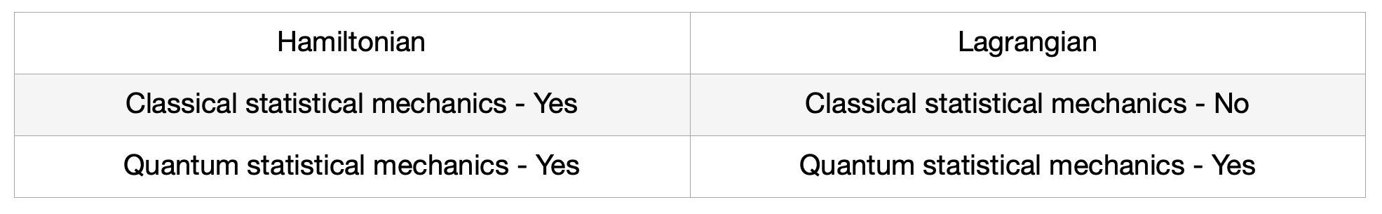
Here comes to a question: “Is there a Lagrangian approach in the classical statistical mechanics ?”. According to a limited knowledge of the author, it seems to be many attempts to make a connection between Lagrangian mechanics and classical statistical mechanics, but not in the similar fashion with those in the Hamiltonian set up. Naively, if one shall try to construct the classical statistical ensemble on the tangent bundle with a given Lagrangian $L(\dot{q},q)=\dot{q}^{2}/2-V(q)$, where $(\dot{q},q)$ is a set of coordinates in tangent bungle and $V(q)$ is a potential energy, it can be immediately noticed that the Lagrangian cannot be used as the energy function $L(\dot{q},q)\neq E$. Therefore, this problem prevents us to proceed further on formulating the ensemble in tangent bundle. One interesting fact is that one can go the quantum level by employing Hamiltonian approach or Lagrangian approach (Feynman path integration with an imaginary time) [3]. Then, this leads to an in-completed big picture, see figure 1, since we do not have a proper Lagrangian formulation in the classical level of the statistical mechanics.

Refer to caption
Figure 1: Hamiltonian and Lagrangian approaches in the classical and quantum statistical mechanics.

In this work, we shall provide a way to formulate the classical statistic ensemble in the tangent bundle. To achieve this goal, the imaginary-time (Wick’s rotation) must be applied. In section 2, the imaginary-time Lagrangian mechanics will be discussed and the classical statistical ensemble in the tangent bundle will be given. A simple example, harmonic oscillator with one degree of freedom, will be used to illustrate the consistent result on computing physical quantities both Hamiltonian and imaginary-time Lagrangian. In section 3, the summary together with some remarks will be mentioned.

2 Imaginary-time Lagrangian mechanics and classical statistical ensemble

In this section, we shall provide a way to construct the classical ensemble directly from the Lagrangian mechanics. For simplicity, we shall consider a system with one degree of freedom and the Lagrangian is given by

$$L(\dot{q},q)=\frac{\dot{q}^{2}}{2}-V(q)\;.$$ (2.1)

It is not difficult to see that, with a standard Euler-Lagrange equation,

$$\frac{\partial L}{\partial q}-\frac{d}{dt}\frac{\partial L}{\partial\dot{q}}=0\;,$$ (2.2)

one obtains

$$\ddot{q}=-\frac{dV}{dq}\;,$$ (2.3)

which is the equation of motion. Under the Wick rotation on time variable: $t\rightarrow i\tau$, the Lagrangian becomes

$$-\mathcal{L}(\tilde{q},q)=\frac{\tilde{q}^{2}}{2}+V(q)\equiv E.$$ (2.4)

where $\tilde{q}=dq/d\tau$. We note that a new Lagrangian in (2.4) can be expressed as $\mathcal{L}(\tilde{q},q)=L(i\tilde{q},q)$. However, we prefer to work with the notion $\mathcal{L}(\tilde{q},q)$ as our convenient and a reason on the invariant of physics 111Otherwise, we have to deal with an imaginary generalised velocity $i\tilde{q}$, presented in the Lagrangian $L(i\tilde{q},q)$. We, therefore, can define a new variable $\bar{q}=i\tilde{q}$ which effectively results the same with a choice $\tilde{q}$. (which will be shortly seen later).

Interestingly, we see that a negative Lagrangian is now a total energy of the system. With (2.4), it is not difficult to see that

$$\tilde{q}=-\frac{\partial\mathcal{L}}{\partial\tilde{q}}\;,$$ (2.5)

and the Euler-Lagrange equation with imaginary time is

$$\frac{\partial\mathcal{L}}{\partial q}+\frac{d}{d\tau}\frac{\partial\mathcal{L}}{\partial\tilde{q}}=0\;,$$ (2.6)

resulting in the equation of motion

$$\tilde{\tilde{q}}=-\frac{dV}{dq}\;,$$ (2.7)

which is invariant under the Wick rotation222Here, we demand the equation of motion remaining the same. Therefore, the modification of the Euler-Lagrange equation is needed resulting in (2.6).. Inserting (2.5) into (2.6), one obtains

$$\tilde{\tilde{q}}=\frac{\partial\mathcal{L}}{\partial q}\;.$$ (2.8)

Remark: Here, we would like to point out that although the Lagrangian (2.4) becomes the total energy of the system, but this Lagrangian must be distinguished from the Hamiltonian, which is also the total energy as well, as follows. The Hamiltonian $H(p,x)$ is a function of the canonical momentum and the generalised coordinate, while the Lagrangian $L(i\tilde{q},q)$ is a function of the imaginary generalised velocity and the generalised coordinate. This results that, with the new Lagrangian (2.4), the dynamics of the system will be expressed on the tangent bundle $(i\tilde{q},q)$ or $(\bar{q},q)$ equipped with a symplectic structure, see right below.

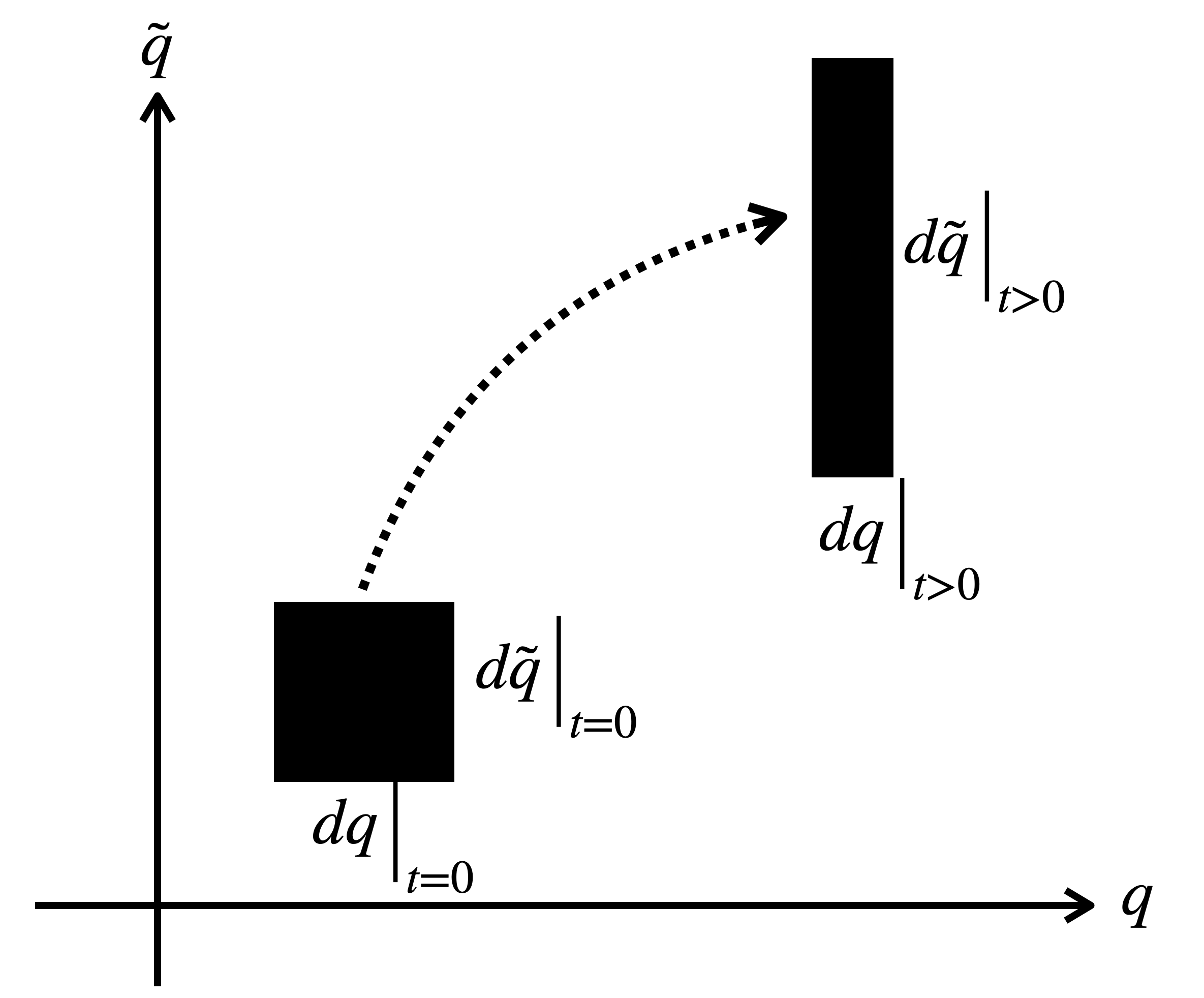
We next would like to show that the area of the tangent bundle preserves under the time evolution. Suppose there is an element area: $d\tilde{q}dq|_{\tau=0}$ and a later time $\tau>0$ area is given by $d\tilde{q}dq|_{\tau>0}$. Using the fact that $q_{\tau}=q_{0}+\tilde{q}d\tau$ and $\tilde{q}_{\tau}=\tilde{q}_{0}+\tilde{\tilde{q}}d\tau$, we have

$\displaystyle d\tilde{q}dq|_{\tau>0}$ $\displaystyle=$ $\displaystyle\left(d\tilde{q}_{0}+d\tilde{\tilde{q}}d\tau\right)\left(dq_{0}+d\tilde{q}d\tau\right)\;.$ (2.9)
$\displaystyle=$ $\displaystyle\left(d\tilde{q}_{0}+\frac{\partial\tilde{\tilde{q}}}{\partial\tilde{q}}d\tilde{q}d\tau\right)\left(dq_{0}+\frac{\partial\tilde{q}}{\partial q}dqd\tau\right)$
$\displaystyle\approx$ $\displaystyle d\tilde{q}dq|_{\tau=0}\left(1+\left(\frac{\partial\tilde{\tilde{q}}}{\partial\tilde{q}}+\frac{\partial\tilde{q}}{\partial q}\right)d\tau\right)\;.$

Using (2.5) and (2.8), equation (2.9) becomes

$\displaystyle d\tilde{q}dq|_{\tau>0}$ $\displaystyle=$ $\displaystyle d\tilde{q}dq|_{\tau=0}\left(1+\left(\frac{\partial}{\partial\tilde{q}}\frac{\partial\mathcal{L}}{\partial q}-\frac{\partial}{\partial q}\frac{\partial\mathcal{L}}{\partial\tilde{q}}\right)d\tau\right)$
$\displaystyle d\tilde{q}dq|_{\tau>0}$ $\displaystyle=$ $\displaystyle d\tilde{q}dq|_{\tau=0}\;.$ (2.10)

Therefore, the area on the tangent bundle is preserved under the time evolution and we shall treat is feature as a Lagrangian version of the Liouville’s theorem, see figure 2.

Refer to caption
Figure 2: Area under the time evolution on the tangent bundle.

It now prompts to define a density function of the states on the tangent bundle: $\rho(\tilde{q},q;\tau)$ and it is not difficult to see that the density function satisfies the equation

$$0=\frac{\partial\rho}{\partial\tau}+\frac{\partial\rho}{\partial q}\frac{\partial q}{\partial\tau}+\frac{\partial\rho}{\partial\tilde{q}}\frac{\partial\tilde{q}}{\partial\tau}=\frac{\partial\rho}{\partial\tau}+\{\rho,\mathcal{L}\}\;,$$ (2.11)

where $\{*,\mathcal{L}\}$ is treated as a Lagrange bracket333We note that this definition of the bracket is not the same with the Lagrangian bracket.

$$\{*,\mathcal{L}\}=\left(\frac{\partial*}{\partial\tilde{q}}\frac{\partial\mathcal{L}}{\partial q}-\frac{\partial*}{\partial q}\frac{\partial\mathcal{L}}{\partial\tilde{q}}\right)\;$$ (2.12)

with a property $\{*,\mathcal{L}\}=-\{\mathcal{L},*\}$. Here, $*$ is a function defined on the tangent bundle. Interesting fact is that the Lagrange bracket (2.12) provides a set of dynamic equations as follows

$\displaystyle\tilde{q}$ $\displaystyle=$ $\displaystyle-\frac{\partial\mathcal{L}}{\partial\tilde{q}}\;,$ (2.13)
$\displaystyle\tilde{\tilde{q}}$ $\displaystyle=$ $\displaystyle\frac{\partial\mathcal{L}}{\partial q}\;,$ (2.14)

which are (2.5) and (2.8), respectively. One can note that a set of (2.13) and (2.14) can be treated as a Lagrange version of the Hamilton’s equations.

Let $dN(\tilde{q},q;\tau)$ be a number of points in an element area $d\tilde{q}dq$ around a point $(\tilde{q},q)$. Then probability density is given by

$$\rho(\tilde{q},q;\tau)d\tilde{q}dq=\lim_{N\rightarrow\infty}\frac{dN}{N}\;,$$ (2.15)

which satisfies the normalisation condition

$$\int_{\Gamma}d\Gamma\rho(\tilde{q},q;\tau)=1\;,\;\;\;d\Gamma=d\tilde{q}dq\;.$$ (2.16)

Any macroscopic quantity can be computed through

$$\langle\mathcal{Q}(\tilde{q},q)\rangle=\int d\Gamma\rho(\tilde{q},q;\tau)\mathcal{Q}(\tilde{q},q)\;,$$ (2.17)

which is treated as an ensemble average. Moreover, the time evolution of the ensemble average is given by

$\displaystyle\frac{d}{d\tau}\langle\mathcal{Q}(\tilde{q},q)\rangle=\int d\Gamma\frac{\partial\rho(\tilde{q},q;\tau)}{\partial\tau}\mathcal{Q}(\tilde{q},q)=\int d\Gamma\mathcal{Q}(\tilde{q},q)\left(\frac{\partial\rho}{\partial\tilde{q}}\frac{\partial\mathcal{L}}{\partial q}-\frac{\partial\rho}{\partial q}\frac{\partial\mathcal{L}}{\partial\tilde{q}}\right)\;.$ (2.18)

Applying integrating by parts, we obatin

$\displaystyle\frac{d}{d\tau}\langle\mathcal{Q}(\tilde{q},q)\rangle$ $\displaystyle=$ $\displaystyle-\int d\Gamma\rho\left[\left(\frac{\partial\mathcal{Q}}{\partial\tilde{q}}\frac{\partial\mathcal{L}}{\partial q}-\frac{\partial\mathcal{Q}}{\partial q}\frac{\partial\mathcal{L}}{\partial\tilde{q}}\right)+\mathcal{Q}\left(\frac{\partial}{\partial\tilde{q}}\frac{\partial\mathcal{L}}{\partial q}-\frac{\partial}{\partial q}\frac{\partial\mathcal{L}}{\partial\tilde{q}}\right)\right]\;.$ (2.19)
$\displaystyle=$ $\displaystyle-\int d\Gamma\rho\{\mathcal{L},\mathcal{Q}\}=\langle\{\mathcal{Q},\mathcal{L}\}\rangle.$

For an equilibrium macroscopic state, the ensemble average does not explicitly depend on time: $\frac{\partial\rho}{\partial\tau}=0$, demanding

$$\{\rho_{eq},\mathcal{L}\}=0\;.$$ (2.20)

This means that a possible solution is for $\rho_{eq}$ to be a function of the Lagrangian: $\rho_{eq}(\mathcal{L}(\tilde{q},q))$. Consequently, one finds that

$$\{\rho_{eq}(\mathcal{L}),\mathcal{L}\}=\rho_{eq}^{\prime}(\mathcal{L})\{\mathcal{L},\mathcal{L}\}=0\;.$$ (2.21)

This means that $\rho$ is constant on the energy surface $E=-\mathcal{L}$, in tangent bundle.

Microcanonical ensemble: For a system with fixed internal energy $U=\langle E\rangle$, volume $V$ and a number of particles $n$, the density function is given by

$$\rho(\tilde{q},q)=\frac{1}{\Sigma}\delta(\mathcal{L}(\tilde{q},q)+U)\;.$$ (2.22)

With the $\int\rho(\tilde{q},q)d\Gamma=1$, it demands

$$\Sigma(U)=\int d\Gamma\delta(\mathcal{L}(\tilde{q},q)+U)\;.$$ (2.23)

Then the ensemble defined on tangent bundle with energy less than or equal $U$ is given by

$$\Omega(U)=\int_{-\mathcal{L}(\tilde{q},q)\leq U}d\Gamma=\int_{0}^{U}dE\Sigma(E)\;.$$ (2.24)

With a given ensemble in (2.24), the classical statistical entropy is given by

$$S(U,V,n)=k_{B}\ln\Omega(U)\;.$$ (2.25)

For two separated systems with $(U_{1},V_{1},n_{1})$ and $(U_{2},V_{2},n_{2})$, the total ensemble is given by $\Omega_{12}=\Omega_{1}\Omega_{2}$ resulting in

$$S_{12}=S_{1}+S_{2}\;,$$ (2.26)

which is known as the additive property of the entropy.

Now, we are ready to make a connection between microscopic and macroscopic worlds. Let’s start with a definition of the temperature

$$\frac{1}{T}=\left(\frac{\partial S}{\partial U}\right)\Big{|}_{V,n}\;.$$ (2.27)
$$dS_{12}=dS_{1}+dS_{2}\;.$$ (2.28)

At equilibrium, $dS_{12}=0$ and $d(U_{1}+U_{2})=0$, one obtains

$$\frac{1}{T_{1}}=\left(\frac{\partial S_{1}}{\partial U_{1}}\right)\Big{|}_{V_{1},n_{1}}=\left(\frac{\partial S_{2}}{\partial U_{2}}\right)\Big{|}_{V_{2},n_{2}}=\frac{1}{T_{2}}\;,$$ (2.29)

which gives a thermal equilibrium condition between two systems or the zeroth law of thermodynamics.

Example: We shall now consider the imaginary-time Lagrangian for the harmonic oscillator

$$-\mathcal{L}(\tilde{q},q;\tau)=\left(\tilde{q}^{2}+q^{2}\right)=E\;.$$ (2.30)

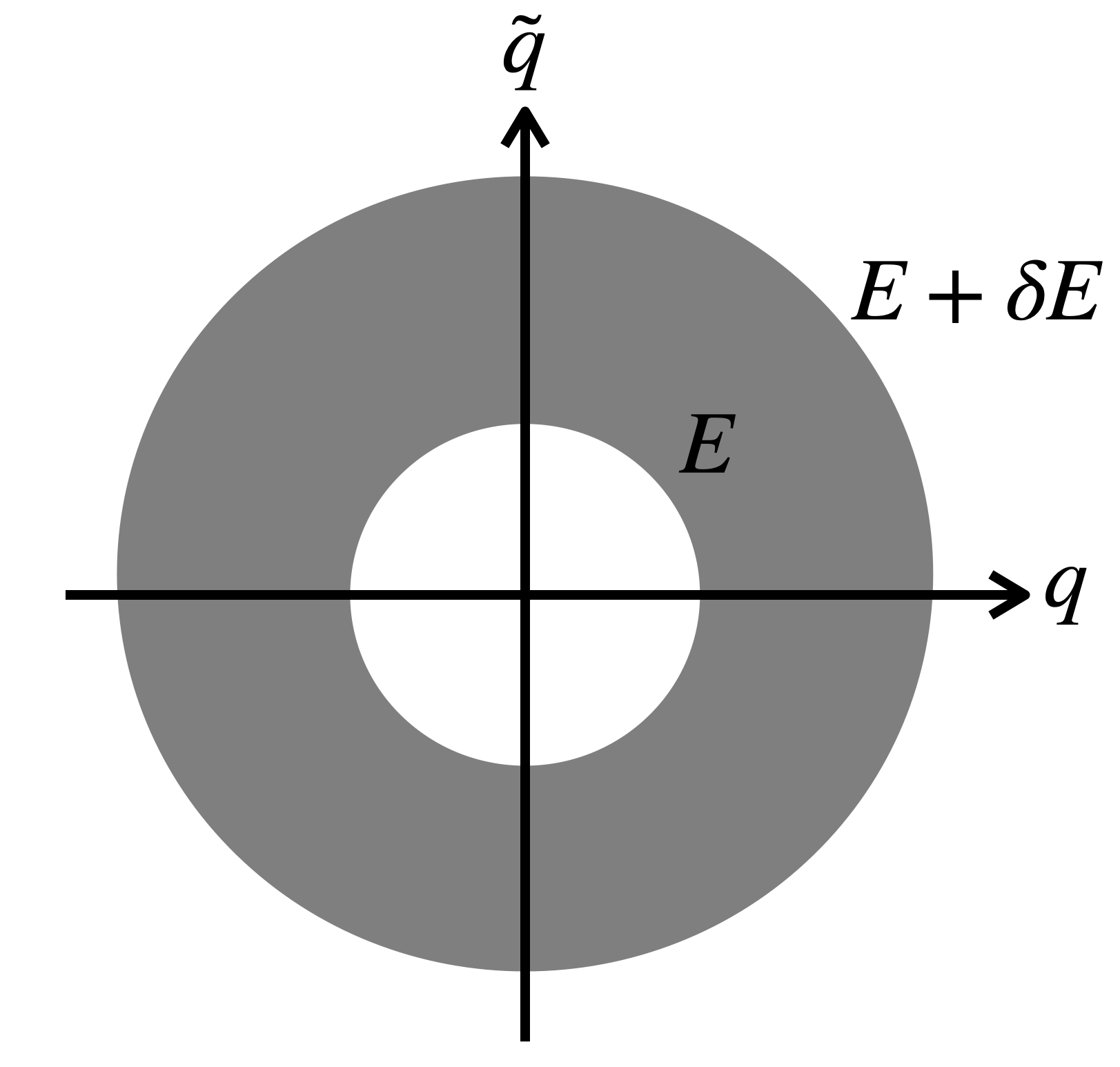
This new form of the Lagrangian allows us to construct the classical ensemble on tangent bundle. In the energy range: $E\rightarrow E+\delta E$, see figure 3, the number of microsates is give by

$$\delta\Omega=2\pi\delta E\;,$$ (2.31)

and, obviously, in the energy range $0\rightarrow E$, the number of microstates is given by

$$\Omega(E)=\frac{1}{h}\int_{0}^{E}d\Omega=\frac{E}{\hbar}\;.$$ (2.32)

Applying the relation $U=\langle E\rangle=k_{B}T$ and the first law $\delta Q=\delta U$, one finds

$$\frac{\delta\Omega}{\Omega}=\frac{\delta U}{U}=\frac{\delta Q}{k_{B}T}\rightarrow dS=\frac{\delta Q}{T}\sim\frac{\delta\Omega}{\Omega}$$ (2.33)

Finally, we find that the entropy is proportional to the total number of microstates: $S=k_{B}\ln\Omega(E)$.

Refer to caption
Figure 3: Ensemble in the energy range $E\rightarrow E+\delta E$ on the tangent bundle.

Canonical ensemble: A system 1 characterised by $(U_{1},V_{1},n_{1})$ is in thermal equilibrium at temperature $T$ with a heat bath, labeled as 2, characterised by $(E_{2},V_{2},n_{2})$ with conditions $E_{2}\gg E_{1}$ and $n_{2}\gg n_{1}$ and $E_{12}=E_{1}+E_{2}$. The condition here is that the energy is allowed to exchange but not of particles. The Lagrangian of the total system is given by

$$\mathcal{L}_{12}(\tilde{q}_{1},\tilde{q}_{2},q_{1},q_{2})=\mathcal{L}_{1}(\tilde{q}_{1},q_{1})+\mathcal{L}_{2}(\tilde{q}_{2},q_{2})\;.$$ (2.34)

Since the total system is isolated, the density function of the total system is given by

$$\rho_{12}(\tilde{q},q)=\frac{1}{\Sigma_{12}}\delta(\mathcal{L}_{12}+E_{12})\;,$$ (2.35)

where $\tilde{q}=(\tilde{q}_{1},\tilde{q}_{2})$ and $q=(q_{1},q_{2})$ and

$$\Sigma_{12}=\int d\Gamma_{12}\delta(\mathcal{L}_{12}+E_{12})\;.$$ (2.36)

Then the classical ensemble is given by

$$\Omega_{12}(E_{12})=\int d\Gamma_{12}\delta(\mathcal{L}_{12}+E_{12})\;.$$ (2.37)

Actually, we are interested in study the property the system 1. Then one has to trace out 2

$\displaystyle\rho_{1}(\tilde{q}_{1},q_{1})$ $\displaystyle=$ $\displaystyle Tr_{2}\rho_{12}(\tilde{q},q)$ (2.38)
$\displaystyle=$ $\displaystyle\frac{\int d\tilde{q}_{2}\int dq_{2}\delta(\mathcal{L}_{1}+\mathcal{L}_{2}+E_{12})}{\Omega_{12}(E_{12})}$
$\displaystyle=$ $\displaystyle\frac{\Omega_{2}(E_{12}+L_{1})}{\Omega_{12}(E_{12})}\;,$

where $\Omega_{2}(E_{2})=\Omega_{12}(E_{12}+\mathcal{L}_{1})$ is a classical ensemble for the system 2. With a condition $E_{1}\ll E_{12}$, one can expand $\ln\Omega_{2}(E_{2})$ around the $E_{2}=E_{12}$ resulting in

$$\ln\Omega_{2}(E_{2})\approx\ln\Omega_{2}(E_{12})+\frac{\partial\ln\Omega_{2}}{\partial E_{2}}\Big{|}_{E_{2}=E_{12}}\mathcal{L}_{1}\;.$$ (2.39)

Since the system 1 and system 2 are in thermal equilibrium with temperature $T$, then we have

$$\Omega_{2}(E_{12}+\mathcal{L}_{1})=\Omega_{2}(E_{12})e^{\frac{\mathcal{L}_{1}}{K_{B}T}}$$ (2.40)

Inserting (2.40) into (2.38), one gets

$$\rho_{1}(\tilde{q}_{1},q_{1})=\frac{\Omega_{2}(E_{12})}{\Omega_{12}(E_{12})}e^{\frac{\mathcal{L}_{1}}{K_{B}T}}=\frac{e^{\beta\mathcal{L}_{1}}}{\int d\Gamma_{1}e^{\beta\mathcal{L}_{1}}}\propto e^{\beta\mathcal{L}_{1}}\;,$$ (2.41)

where $e^{\beta\mathcal{L}_{1}}$ will be treated as a Lagrangian version of the Boltzmann factor and $\beta=\frac{1}{k_{B}T}$.

What we have now is that, for any system with thermal equilibrium with surrounding, the density function is given by

$$\rho(\tilde{q},q)=\frac{e^{\beta\mathcal{L}(\tilde{q},q)}}{\int d\Gamma e^{\beta\mathcal{L}(\tilde{q},q)}}\;,$$ (2.42)

and the canonical partition function $Z$ is defined as

$$Z\equiv-\frac{1}{h}\int d\Gamma e^{\beta\mathcal{L}(\tilde{q},q)}\;.$$ (2.43)

Next, we consider

$\displaystyle\frac{\partial}{\partial\beta}\ln Z$ $\displaystyle=$ $\displaystyle-\frac{\int d\Gamma(\mathcal{L})e^{\beta L}}{\int d\Gamma e^{\beta\mathcal{L}}}$ (2.44)
$\displaystyle=$ $\displaystyle\langle-\mathcal{L}\rangle=U\;.$

Then we employ the relation $U=\frac{\partial}{\partial\beta}(\beta F)$, where $F$ is the Helmholtz free energy. The final relation is

$$Z=e^{\beta F}\;,\;\;\text{or}\;\;F(T,V,n)=k_{B}T\ln Z(T)\;.$$ (2.45)

Example: We shall work out with the harmonic oscillator with one degree of freedom again. The partition is given by

$$Z=-\frac{1}{h}\int_{-\infty}^{+\infty}d\tilde{q}\int_{-\infty}^{+\infty}dqe^{\beta(\tilde{q}^{2}+q^{2})}=\frac{k_{B}T}{\hbar}\;,$$ (2.46)

which is identical with the Hamiltonian approach.

3 Concluding summary

We successfully provide a systematical way on constructing the classical statistical ensemble in the tangent bundle $(i\tilde{q},q)$. A magic trick used here is the Wick’s rotation from the real time to the imaginary time on the Lagrangian. This transformation gives a couple of first order differential equations which can be viewed as the Lagrangian analogue of the Hamilton’s equations. With this new structure on tangent bundle equipped with imaginary-time, the area under the consideration does not change under the time evolution and, of course, this feature could be considered as the Lagrangian version of the Liouville’s theorem in tangent bundle. Throughout these processes, one can naturally construct the statistical ensemble in tangent bundle, which now possesses the symplectric structure through the object $dq\wedge d\tilde{q}$, and an important quantity in this context known as the statistical entropy or Boltzmann entropy is constructed. With a well known example, harmonic oscillator with one degree freedom, one can show that both approaches, Hamiltonian and imaginary-time Lagrangian, give identical result on computing physical quantities, i.e. entropy and canonical partition function. We hope very much that, with this preliminary work on a quadratic case of the kinetic term 444Here, in this work, we focus on non-relativistic cases., the missing piece in figure 1 is filled and completes a whole picture. Moreover, with this alternative approach on the Lagrangian side, new mathematical features might be possibly explored leading a new play ground on studying physics.

Acknowledgements

S. Yoo-Kong would like to express a depth of gratitude to colleagues for valuable discussions.

References

  • [1] Flamm D, 1998, History and outlook of statistical physics, arXiv:physics/9803005.
  • [2] Reif F, 2009, Fundamentals of Statistical and Thermal Physics, Waveland Press.
  • [3] Feymann R P, 1972, Statistical Mechanics. A set of lectures (Frontiers in physics), London, United Kingdom: Perseus Books.