Generalizable Heterogeneous Federated Cross-Correlation and Instance Similarity Learning

Abstract

Federated learning is an important privacy-preserving multi-party learning paradigm, involving collaborative learning with others and local updating on private data. Model heterogeneity and catastrophic forgetting are two crucial challenges, which greatly limit the applicability and generalizability. This paper presents a novel FCCL+, federated correlation and similarity learning with non-target distillation, facilitating the both intra-domain discriminability and inter-domain generalization. For heterogeneity issue, we leverage irrelevant unlabeled public data for communication between the heterogeneous participants. We construct cross-correlation matrix and align instance similarity distribution on both logits and feature levels, which effectively overcomes the communication barrier and improves the generalizable ability. For catastrophic forgetting in local updating stage, FCCL+ introduces Federated Non Target Distillation, which retains inter-domain knowledge while avoiding the optimization conflict issue, fulling distilling privileged inter-domain information through depicting posterior classes relation. Considering that there is no standard benchmark for evaluating existing heterogeneous federated learning under the same setting, we present a comprehensive benchmark with extensive representative methods under four domain shift scenarios, supporting both heterogeneous and homogeneous federated settings. Empirical results demonstrate the superiority of our method and the efficiency of modules on various scenarios. The benchmark code for reproducing our results is available at https://github.com/WenkeHuang/FCCL.

1 Introduction

Current deep neural networks have enabled great success in various computer vision tasks [2, 3], based on the large-scale and computationally expensive training data [4, 5, 6]. However, in real world, data are usually distributed across numerous participants (e.g., mobile devices, organizations, cooperation). Due to the ever-rising privacy concerns and strict legislations [7], the traditional center training paradigm which requires to aggregate data together, is prohibitive. Driven by such realistic challenges, federated learning [8, 9, 10, 11] has been popularly explored as it can train a global model for different participants rather than centralize any private data. Therefore, it provides an opportunity for privacy-friendly collaborative machine learning paradigm and has shown promising results to facilitate real world applications, such as keyboard prediction [12], medical analysis[13] and humor recognition [14].

Figure 1: Problem illustration of heterogeneous federated learning. (a) In collaborative updating, how to handle the communication problem of heterogeneous models and learn a generalizable representation under heterogeneous data (domain shift)? (b) In local updating, how to effectively alleviate catastrophic forgetting to present stable and satisfactory performance in both inter- and intra-domains?

Despite the great success afforded by federated learning, there remains fundamental research problems [15]. One key challenge is data heterogeneity [16, 17]. In practical, private data distributions from different participants are inherently non-i.i.d (independently and identically distributed) since data are usually collected from different sources under varying scenarios. Existing works [18] have indicated that under heterogeneous data, standard federated learning methods such as FedAvg [8] inevitably faces performance degradation or even collapse. A resurgence of methods mainly focus on incorporating extra proximal terms to regularize the local optimization objective close to the global optima [19, 20, 21]. However, they ignore the fact that there exists domain shift, where the private data feature distribution of different participants may be strikingly distinct [22, 23, 24]. Thus, the optimization objective is required to ensure both generalization performance on others domains and discriminability ability on itself domain. However, existing methods mostly focus on facilitate performance on intra-domain and would suffer from drastic performance drop on others domains with disparate feature distribution. As a result, forcing private model to acquire generalizable ability under domain shift is important and meaningful. The other inescapable and practical challenge is model heterogeneity. Specifically, participants have the option of architecting private models rather than agreeing on the pre-defined architecture because they may have different design criteria, distinctive hardware capability [25] or intellectual property rights [26]. Thus, taking into account data heterogeneity and model heterogeneity together, previously aforementioned methods are no longer feasible because they are based on sharing consistent model architecture for parameter averaging operation. In order to address this problem, existing efforts can be taxonomized into two major categories: shared global model [27, 28, 29] and knowledge transfer [30, 31, 32, 33, 34]. However, leveraging extra global model not only raises the communication cost but also necessitates additional model structure in participant side. For knowledge transfer methods, provided with unlabeled public data or artificially generated data, they utilize knowledge distillation [35, 36] to transfer the logits output on public data among participants. However, this strategy is subject to a significant limitation: they conduct knowledge transfer via logits output, which is in high semantic level [37]. Directly aligning distribution probably provides confusing optimization direction [38, 39] since the category of public data is unknowable and is possible inconsistent with private data. Thus, considering data and model heterogeneity together, an essential issue has long been overlooked: (a) How to achieve a better generalizable representation in heterogeneous federated learning? This problem is shown in Fig. 1 (a).

Besides, in domain shift, data are typically from various domains. Thus, private models are required to maintain satisfactory performance not only on the intra-domain but also on the inter-domain. However, a major hindrance is derived from the federated learning paradigm. In general, federated learning could be regarded as a cyclic process with two steps: collaborative updating and local updating [8, 9]. Specifically, during collaborative updating, participants learn from others and incorporate inter-domain knowledge and probably overlap intra-domain ability. Then in local updating, the model is solely trained on private data. If optimized for too many epochs, it would be prone to overfit intra-domain knowledge and forgets previously learned inter-domain knowledge, leading to inter-domain catastrophic forgetting. In contrast, with too limited training epochs, it would perform poorly in the intra-domain, resulting in intra-domain catastrophic forgetting. Collaboratively considering the above two cases, catastrophic forgetting [40, 41, 42] presents an important obstacle towards learning a generalization model in heterogeneous federated learning. Related methods mainly focus on introducing parameter stiffness to regulate learning objective [19, 20, 43, 21, 34], which either rely on model homogeneity or do not take full advantage of the underlying inter-domain knowledge provided from models which are optimized in collaborative learning. Consequently, a natural question arises: (b) How to effectively balance multiple domains knowledge to alleviate catastrophic forgetting? An illustration of these two problems is presented in the Fig. 1.

To acquire generalization ability in heterogeneous federated learning, inspired by self-supervised learning with information maximization[44, 45, 46], a preliminary version of this work published in CVPR 2022 [1] explores Federated Cross-Correlation Matrix (FCCM). In particular, we aim to make same dimensions of logits output highly correlated to learn class invariance and decorrelate pairs of different dimensions within logits output to stimulate the diversity of different classes. Moreover, representation (embedding feature) exhibits generic information related to structural information [47], but is in lack of effective utilization. This motivates us to capture more significant information in other participants models representation. We propose Federated Instance Similarity Learning (FISL), which leverages unlabeled public data to innovatively align instance similarity distribution among participants. Specifically, for each unlabeled public instance, private model calculates feature vector and obtains its similarity with respect to other instances in the same batch. We convert the individual feature distribution into similarity probability distribution. Then, we transfer that knowledge, so that participants are required to mimic the same similarity distribution. This approach offers a practical solution to realize feature level knowledge communication for differential feature under model heterogeneous federated learning. Besides, we believe that FCCM is essential because it optimizes classifier in collaborative learning to alleviate its bias towards local data distribution [48, 49]. To this end, we develop both Federated Cross-Correlation Matrix and Federated Instance Similarity Learning modules in heterogeneous federated learning, which handle the communication problem for heterogeneous models via achieving both logits and feature-level knowledge communication to acquire a more generalizable representation in heterogeneous federated learning.

To alleviate inter-domain knowledge forgetting in local updating, we propose a heterogeneous distillation to extract useful knowledge from respective previous model after communicating with other participants, which captures inter-domain knowledge. To maintain intra-domain discriminability, we intuitively leverage label supervision [50]. However, there exists optimization conflict when simultaneously maintaining inter- and intra-domains knowledge. Specifically, we observe that typical knowledge distillation [36, 51] can be viewed as target distillation (ground-truth class prediction) and non-target distillation (residual classes prediction component). We conjecture that non-target distillation depicts the classes relation provided by previous model which contains privileged inter-domain information [52, 53]. For target distillation, it concentrates on intra-domain knowledge since it represents the specific prediction on ground-truth label. However, previous model could not consistently provide higher confidence on target class than current updating model, leading to contradictory gradient direction with respective label. In our conference version [1], we leverage pretrained intra-domain model to alleviate this problem because it normally presents high confidence on target label, offering stable constraint. In this journal version, we propose Federated Non Target Distillation (FNTD) to separately distill non-target information from previous model, which better preserves inter-domain knowledge and ensures generalization ability while improving intra-domain discriminability. Compared with our conference version, FNTD not only avoids the requirement of a well-pretrained model but also improves the efficiency of inter-domain knowledge transfer in local updating.

This paper builds upon on our conference paper [1] with extended contributions, which are listed in the following:

• We introduce an effective heterogeneous feature knowledge transfer strategy in federated learning, Federated Instance Similarity Learning (FISL), to build the connection among heterogeneous participants without additional shared network structure design. Through aligning the instance similarity distribution among unlabeled public data, heterogeneous models realize feature information communication. Collaborated with proposed Federated Cross-Correlation Matrix (FCCM), we realize both logits and feature levels knowledge communication, resulting in better generalizable ability.

• We disentangle the typical knowledge distillation and develop Federated Non Target Distillation (FNTD) to better preserve inter-domain knowledge in the local updating stage. Cooperated with private data label supervision (intra-domain information) constraint, it effectively balances multiple domains knowledge and thus addresses the catastrophic forgetting problem, improving both inter- and intra-domains performance.

• We provide a unified benchmark for both heterogeneous and homogeneous federated learning, supporting various state-of-the-art methods. We rigorously validate proposed method on massive scenarios (i.e., Digits [54, 55, 56, 57], Office Caltech [58], Office31 [59] and Office-Home [60]) with unlabeled public data (i.e., Cifar-100 [61], Tiny-ImageNet [4] and Fashion-MNIST [62]). We further provide detailed ablation studies and in-depth discussions to validate its effectiveness.

2 Related Work

2.1 Heterogeneous Federated Learning

Data Heterogeneity. A pioneering work proposed the currently most widely used algorithm, FedAvg[8]. But it suffers performance drop on non-i.i.d data (data heterogeneity). Shortly after, a large body methods [19, 20, 43, 21, 34, 63, 64] research on non-i.i.d data. These methods mainly focus on label skew with limited domain shift. However, when private data sampled from different domains, these works do not consider inter-domain performance but only focus on learning an internal model. Latest researches have studied related problems on domain adaptation for target domain [65] and domain generalization for unseen domains [13]. However, collecting enough data in target domain can be time-consuming. Meanwhile, considering the performance on unknown domains is an idealistic setting. For more realistic settings, participants are probably more interested in the performance on others domains, which could directly improve economic benefits. In this paper, we focus on improving inter-domain performance under domain shift.

Model Heterogeneity. With the demand for unique models, model heterogeneous federated learning has been an active research field. One Direction is introducing shared extra model [27, 29]. However, these techniques may not be applicable when considering additional computing overhead and expensive communication cost. Recently, A line of work [30, 31, 66] operates on labeled public data (with similar distribution) via knowledge distillation [35, 36]. Therefore, these approaches heavily rely on the quality of labeled public data, which may not always be available on the server. Latest works [32, 67, 68] have proven the feasibility to do distillation on unlabeled public data or synthetic data. However, these methods reach semantic information consistency on unlabeled public data, which are not suitable to learn a generalizable representation and thus lead to a sub-optimal inter-domain performance. In this paper, based on unlabeled public data, we construct cross-correlation matrix and measure instance similarity on unlabeled public data to reach generalizable ability.

2.2 Catastrophic Forgetting

Catastrophic forgetting [41, 42] has been an essential problem in incremental learning [69, 70] when models continuously learn from a data stream, with the goal of gradually extending acquired knowledge and using it for future [40, 42]. Existing incremental learning works can be broadly divided into three branches [71]: replay methods [72, 73], regularization-based methods [74, 75] and parameter isolation methods [76, 77]. As for federated learning, data are distributed rather than sequential like incremental learning. Despite these differences, both incremental learning and federated learning share a common challenge - how to balance the knowledge from the different data distributions. Unlike incremental learning methods, we focus on alleviating catastrophic forgetting in distributed data rather than time series data. In particular, we expect to alleviate both inter- and intra-domains catastrophic forgetting in the local updating stage to acquire a generalization model.

2.3 Self-Supervised Learning

Self-supervised learning has emerged as a powerful method for learning useful representation without supervision from labels, largely reducing the performance gap between supervised models on various downstream vision tasks. Many related methods are based on contrastive methods [78, 79, 80, 81, 82]. This kind method contrasts positive pairs against negative pairs, where positive pairs are often formed by same samples with different data augmentations and negative pairs are normally other different samples. Recently, another line of works [83, 84] employs asymmetry of the learning update (stop-gradient operation) to avoid trivial solutions. Besides, a principle to prevent collapse is to maximize the information content of the embeddings [44, 45, 46]. The key difference between Federated Cross-Correlation Matrix (FCCM) and aforementioned efforts is that ours is designed for federated setting rather centralized setting. Inspired by self-supervised learning, We construct the comparison among heterogeneous models in federated learning.

2.4 Knowledge Distillation

Knowledge distillation aims to transfer knowledge from one network to the other [35, 36]. The knowledge from the teacher network can be extracted and transferred in various ways. Related approaches can be mainly divided into three directions: logits distillation [36, 85, 86, 37], feature distillation [87, 88] and relation distillation [89, 90]. In this work, we propose Federated Instance Similarity Learning (FISL) to implement multi-party rather than pair-wise heterogeneous feature communication in collaborative updating. Furthermore, we investigate how to better maintain inter-domain knowledge in local updating and develop Federated Non Target Distillation (FNTD) to disentangle logits distillation, which assures inter-domain performance without the heavy computational strain.

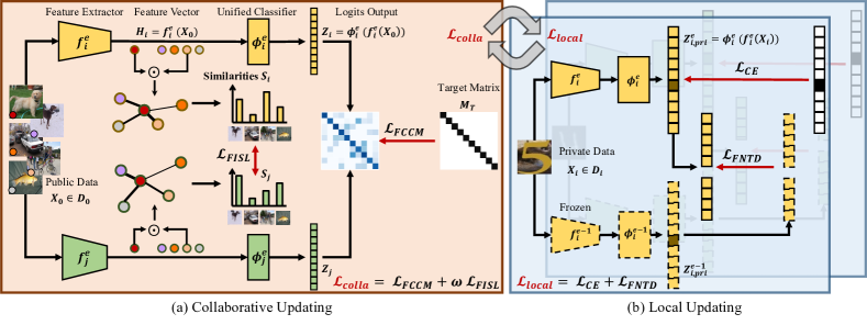
Figure 2: Schematization of FCCL+. Our method solves heterogeneity problem and catastrophic forgetting in federated learning. (a) Collaborative updating: we propose Federated Cross-Correlation Matrix (FCCM § 3.1) via constructing cross-correlation matrix $\mathcal{M}_{i}$ to target matrix, $\mathcal{M}_{T}=2\times eye(C)-ones(C)$, where on-diagonal is $1$, off-diagonal is $-1$. Besides, we introduce Federated Instance Similarity Learning (FISL § 3.2) to realize heterogeneous feature communication. (b) Local updating: we decouple typical knowledge distillation and develop Federated Non Target Distillation (FNTD § 3.3) to better preserve inter-domain knowledge. Moreover, we leverage private data label signal to maintain intra-domain performance. Best viewed in color. Zoom in for details.

3 Methodology

Problem Statement and Notations. Following the standard federated learning setup, there are $K$ participants (indexed by $i$). The $i^{th}$ participant has a local model $\theta_{i}$ and private data $D_{i}=\{(X_{i},Y_{i})|X_{i}\in\mathbb{R}^{N_{i}\times O},Y_{i}\in\mathbb{R}^{N_{i}\times C}\}$, where $N_{i}$ denotes the scale of private data, $O$ represents input size and $C$ is defined as classification categories. We further consider local model as two components: feature extractor and unified classifier. The feature extractor $f:\mathcal{X}\rightarrow\mathcal{H}$, maps input image $x$ into a compact $d$ dimensional feature vector $H=f(x)\in\mathbb{R}^{d}$. A unified classifier $\phi:\mathcal{H}\rightarrow\mathcal{Z}$, produces probability output, $Z=\phi(f(x))\in\mathbb{R}^{C}$ as prediction for $x$. Thus, the overall private model is denoted as $\theta_{i}=(f_{i},\phi_{i})$. In heterogeneous federated learning, data heterogeneity and model heterogeneity are defined as:

• Data heterogeneity: $P_{i}(X|Y)\neq P_{j}(X|Y)$. There exists domain shift among private data, i.e., conditional distribution $P(X|Y)$ of private data vary across participants even if $P(Y)$ is shared. Specifically, the same label $Y$ has distinctive feature $X$ in different domains.

• Model heterogeneity: $Shape(\theta_{i})\neq Shape(\theta_{j})$. Participants architect models independently, i.e., the feature extractor $f$ are different such as ResNet[3], EfficientNet[91] and MobileNet[92], and the corresponding classifier module is also differential.

The unlabeled public dataset $D_{0}=\{X_{0}|X_{0}\in\mathbb{R}^{N_{0}\times O}\}$ is adopted to achieve heterogeneous models communication, which is relatively easy to access in real scenarios, e.g., existing datasets [5, 4, 6] and web images[93]. The goal for $i^{th}$ participant is to reach communication and learn a model $\theta_{i}$ with generalizable ability. Besides, with catastrophic forgetting, the optimization objective is to present both higher and stabler inter- and intra-domains performance. We provide the notation table in Tab. I for better understanding.

TABLE I: Notations table.

	Description		Description
$K$	Participant scale	$i$	Participant index
$D_{i}$	Private data set of $i$ client	$B_{0}$	Private data $D_{i}$ batch
$C$	Classification categories	$O$	Input size
$\theta$	Neural network	$f$	Feature extractor
$\phi$	Unified classifier	$H$	Feature embedding
$Z$	Logits output	$d$	Feature dimension
$N_{i}$	Scale of $D_{i}$	$D_{0}$	Unlabeled public data
$B_{0}$	Public data $D_{0}$ batch	$M_{i}$	Cross-correlation matrix (Eq. 1)
$S_{i}$	Instance similarity distribution(Eq. 3)	$\mathbf{p}$	Predictive distribution (Eq. 7)
$E$	Communication epochs	$T$	Local rounds

3.1 Federated Cross-Correlation Matrix

Motivation of Dimension-Level Operation. Motivated by information maximization [94, 45, 46], a generalizable representation should be as informative as possible about image, while being as invariant as possible to the specific domain distortions that are applied to this sample. In our work, domain shift leads distinctive feature $X$ for the same label $Y$ in different domains. Therefore, the distribution of logits output along the batch dimension in different domains is not identical. Moreover, different dimensions of logits output are corresponding to distinct classes. Thus, we encourage the invariance of the same dimensions and the diversity of different dimensions. Private data carries specific domain information and is under privacy protection, which is not suitable and feasible to conduct collaborative updating. Therefore, we leverage unlabeled public data, which are normally generated and collected from multi domains. Hence, private models are required to reach logits output invariant to domain distortion and decorrelate different dimensions of logits output on unlabeled public data.

Construct Federated Cross-Correlation Matrix. Specifically, we obtain the logits output from $i^{th}$ participant: $Z_{i}=\phi(f(X_{0}))\in\mathbb{R}^{|B_{0}|\times C}$ on unlabeled public data $D_{0}(X_{0})$ with batch $B_{0}$. For $i^{th}$ and $j^{th}$ participant, the logits output is $Z_{i}$ and $Z_{j}$, respectively. Notably, considering the computing burden on the server side, we calculate average logits output: $\overline{Z}=\frac{1}{K}\sum_{i}Z_{i}$. Then, we calculate cross-correlation matrix, $\mathcal{M}_{i}$ for $i^{th}$ participant with average logits output as:

$$\small\mathcal{M}_{i}^{uv}\triangleq\frac{\sum_{b}(\Phi(Z_{i})^{b,u}~{}~{}\Phi(\overline{Z})^{b,v})}{\sqrt{\sum_{b}{\Phi(Z_{i})^{b,u}}^{2}}\sqrt{\sum_{b}{\Phi(\overline{Z})^{b,v}}^{2}}}.$$ (1)

The $b$ indexes batch samples, $u,v$ index the dimension of logits output and $\Phi$ is the normalization operation along the batch dimension with mean subtraction. $\mathcal{M}_{i}$ is a square matrix with size of output dimensionality, $C$ and is comprised between -1 (i.e., dissimilarity) and 1 (i.e., similarity). Then, the FCCM loss for $i^{th}$ participant is defined as:

$$\small\mathcal{L}_{{{FCCM}}}={\sum_{u}(1-\mathcal{M}_{i}^{uu})^{2}}+\lambda{\sum_{u}\sum_{v\neq u}{(1+\mathcal{M}_{i}^{uv}})^{2}},$$ (2)

where $\lambda$ is a positive constant trading off the importance of the first and second terms of loss. Naturally, when on-diagonal terms of the cross-correlation matrix take the value $+1$, it encourages the logits output from different participants to be similar; when off-diagonal terms of the cross-correlation matrix take value $-1$, it encourages the diversity of logits output since different dimensions of these logits output will be uncorrelated to each other.

Comparison with Analogous Methods. FedMD [30] minimizes mean square error on relative public data with annotation. FedDF [32] reaches logits output distribution consistency on unlabeled public data. However, FCCM expects to achieve correlation of same dimensions but decorrelation of different dimensions on unlabeled public data. Besides, we operate along the batch dimension, which means that we view unlabeled public data as ensemble rather than individual sample. It is advantageous to eliminate anomalous sample disturbance. We further illustrate the conceptual comparison between FedDF and FCCM in Fig. 3.

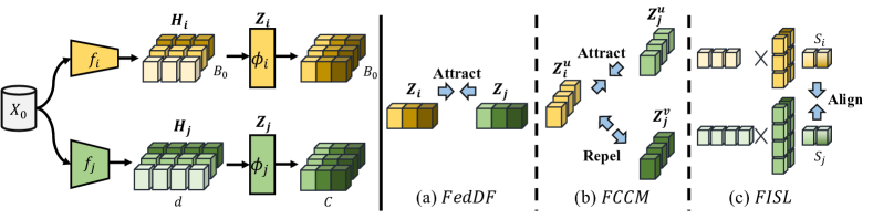
Figure 3: Conceptual Illustration. The unlabeled public data $D_{0}(X_{0})$ with batch size $B_{0}$ are fed into different models. The feature vector $H_{i}=f_{i}(X_{0})$ has $d$ dimensions, which is inconsistent for different models. The logits output $Z_{i}=\phi_{i}(f_{i}(X_{0}))$ has $C$ dimensions, which is same due to the consistent classification categories. (a) FedDF[32] calculates the distribution divergence where instance-wise normalized logits output is compared inside a batch. (b) FCCM [1] learns invariance in same dimensions and decorrelates pairs of different dimensions on the batch-wise normalized logits output in Eq. 1. Thus, for each local logits dimensional output, it aims to attract with same dimension and repel different dimensions with other clients See § 3.1 for details. (c) FISL further leverages feature vector to calculate instance similarity distribution $S_{i}$ by Eq. 3 and Eq. 4. Then, optimize present model to align it with others via Eq. 5. See § 3.2 for details. Best viewed in color.

Input: Communication epochs $E$, local rounds $T$, participants number $K$, unlabeled public data $D_{0}(X_{0})$, $i^{th}$ private data $D_{i}(X_{i},Y_{i})$ , hyper-parameter $\lambda,\mu,\omega,\tau$

for $e=1,2,...,E$ do

      

      for $i=1,2,...,K$ do

             $H_{i}=f_{i}^{e}(X_{0})$ ;

              // feature vector

             $Z_{i}=\phi_{i}^{e}(H_{i})$ ;

              // logits output

             $S_{i}\leftarrow(H_{i},\mu)$ by Eq. 3 and Eq. 4 ;

              // instance similarity

            

      

      $\overline{S}=\frac{1}{K}\sum_{i}S_{i}$  $\overline{Z}=\frac{1}{K}\sum_{i}Z_{i}$

      for $i=1,2,...,K$ in parallel do

            

            $\mathcal{L}_{{{FCCM}{}}}\leftarrow$ Federated Cross-Correlation Matrix ($Z_{i}$, $\overline{Z}$)

            $\mathcal{L}_{{{FISL}{}}}\leftarrow$ Federated Instance Similarity Learning ($S_{i}$, $\overline{S}$)

            $\mathcal{L}_{colla}=\mathcal{L}_{{{FCCM}{}}}+\omega\mathcal{L}_{{{FISL}{}}}$ (Eq. 6)

            $\theta_{i}^{e}\leftarrow\theta_{i}^{e}-\eta\nabla\mathcal{L}_{colla}$

            $\theta_{i}^{e+1}\leftarrow$ Federated Non Target Distillation ($\theta_{i}^{e-1}$, $D_{i}$)

      

return $\theta_{i}^{E+1}$

Federated Cross-Correlation Matrix ($Z_{i}$, $\overline{Z}$)

See details in § 3.1

$\mathcal{M}_{i}\leftarrow(Z_{i},\overline{Z})$ by Eq. 1

$\mathcal{L}_{{FCCM}{}}\leftarrow(\mathcal{M}_{i},\lambda)$ through Eq. 2

return $\mathcal{L}_{{FCCM}{}}$

Federated Instance Similarity Learning ($S_{i}$, $\overline{S}$)

See details in § 3.2

$\mathcal{L}_{{FISL}{}}\leftarrow(S_{i},\overline{S})$ via Eq. 5

return $\mathcal{L}_{{FISL}{}}$

Federated Non Target Distillation ($\theta_{i}^{e-1}$, $D_{i}$):

See details in § 3.3

for $t=1,2,...,T$ do

      

      $Z_{i,pri}^{e}=\phi_{i}^{e}(f_{i}^{e}(X_{i}))$

      $\mathcal{L}_{CE}\leftarrow\texttt{CE}(Z_{i}^{e},Y_{i})$ in Eq. 9

      $Z_{i,pri}^{e-1}=\phi_{i}^{e-1}(f_{i}^{e-1}(X_{i}))$

      $\mathcal{L}_{{FNTD}{}}\leftarrow(Z_{i,pri}^{e},Z_{i,pri}^{e-1},\tau)$ by Eq. 13

      $\mathcal{L}_{local}=\mathcal{L}_{CE}+\mathcal{L}_{{FNTD}{}}$ (Eq. 14)

      $\theta_{i}^{e}\leftarrow\theta_{i}^{e}-\eta\nabla\mathcal{L}_{local}$

$\theta_{i}^{e+1}\leftarrow\theta_{i}^{e}$

return $\theta_{i}^{e+1}$

Algorithm 1 FCCL+

3.2 Federated Instance Similarity Learning

Feature-Level Communication Dilemma. It is known that embedding feature can be convenient to express many generic priors about the world [95, 47], i.e., priors that are not task-specific but would be likely to be useful for generalization ability. Intuitively, it is beneficial to conduct feature-level communication in federated learning. However, in model heterogeneous federated learning, embedding features are in distinctive structure for different participants.

Instance-wise Similarity. Due to the heterogeneous feature, we formulate a novel and simple approach for the feature-wise communication on the basis of instance similarity distribution on unlabeled public data. Formally, given $B_{0}$ a batch of unlabeled public data $D_{0}$, the $i^{th}$ private model $\theta_{i}$ maps them into the embedding feature vector $H_{i}=f(B_{0})\in\mathbb{R}^{|B_{0}|\times d}$. Let $S_{i}$ represents the similarity distribution of feature vector among unlabeled public data batch computed by the $i^{th}$ private model and is defined as:

$$\small\begin{split}S_{i}\triangleq\frac{H_{i}\cdot H_{i}^{T}}{\mu||H_{i}||_{2}||H_{i}||_{2}}\in\mathbb{R}^{|B_{0}|\times|B_{0}|},\end{split}$$ (3)

where $||\cdot||_{2}$ represents $\ell_{2}$ norm, $\mu$ is the soften hyper-parameter, $(\ )^{T}$ denotes transpose operation and $(\ \cdot\ )$ means inner product. Note that, we eliminate the diagonal value in $S_{i}$, which is the similarity value with itself and poses large value, resulting in dominant effect for the whole similarity distribution. Hence, the $S_{i}$ is rewritten into:

$$\small\begin{split}S_{i}&=S_{i}\odot\left[\begin{array}[]{cccc}0&1&\cdots&1\\ 1&0&\cdots&1\\ \vdots&\vdots&\ddots&1\\ 1&1&1&0\end{array}\right]\\ S_{i}&=S_{i}[S_{i}\neq 0]\in\mathbb{R}^{(|B_{0}|-1)\times(|B_{0}|-1)}.\end{split}$$ (4)

Similarly, it is important to control the server-side computing overhead, we measure the average similarity distribution: $\overline{S}=\frac{1}{K}\sum_{i}S_{i}$. Finally, the Federated Instance Similarity Learning (FISL) optimization objective for $i^{th}$ participant is:

$$\small\mathcal{L}_{{FISL}{}}=\sigma(\overline{S},dim\!=\!1)\log\frac{\sigma(\overline{S},dim\!=\!1)}{\sigma(S_{i},dim\!=\!1)},$$ (5)

where $\sigma$ denote softmax function. As shown in Eq. 5, We achieve the purpose of feature-level knowledge communication in model heterogeneous federated learning and lean more versatile information from others, bringing better generalizable ability. We further illustrate FISL in Fig. 3.

Overall Objective in Collaborative Updating. By combining $\mathcal{L}_{{FCCM}{}}$ in Eq. 2 and $\mathcal{L}_{{FISL}{}}$ in Eq. 5, the overall training target in collaborative updating becomes:

$$\small\mathcal{L}_{colla}=\mathcal{L}_{{FCCM}{}}+\omega\mathcal{L}_{{FISL}{}}.$$ (6)

3.3 Federated Non Target Distillation

Typical Knowledge Distillation. Leveraging the previous model optimized in collaborative learning to conduct knowledge distillation on present updating model is beneficial to alleviate inter-domain knowledge forgetting in local updating. Existing knowledge distillation mainly follow three lines: feature distillation, relation distillation and logits distillation [96]. However, compared with collaborative updating phase where major computational cost is allocated to server rather participants, in local updating phase, private models are required to train for multiple epochs and the first two distillation methods pose markedly larger computational cost than logits distillation. Thus, leveraging logits knowledge distillation is feasible and practical in local updating. We denote $\mathcal{T}$ and $\mathcal{S}$ as teacher and student models. The logits knowledge distillation loss is defined as:

$$\small\begin{split}\mathcal{L}_{{KD}}&=\text{KL}(\mathbf{p}_{\mathcal{T}}||\mathbf{p}_{\mathcal{S}})\\ {\mathbf{p}(x,\theta)}&=[{p}^{1},..,{p}^{t},..,{p}^{C}]\in\mathbb{R}^{1\times C},\end{split}$$ (7)

$$\small\begin{split}\mathcal{L}_{{KD}}&=\sum_{u}^{C}p_{\mathcal{T}}^{u,\tau}\log(\frac{p_{\mathcal{T}}^{u,\tau}}{p_{\mathcal{S}}^{u,\tau}})\\ p^{u,\tau}(x,\theta)&=\frac{\exp(z^{u}/\tau)}{\sum_{v}^{C}\exp(z^{v}/\tau)},z=\phi(f(x)),\end{split}$$ (8)

where $z^{u}$ represents the logits output of $u^{th}$ class and $\tau$ is temperature hyper-parameter. Besides, in local updating period, leveraging private data label to construct CrossEntropy [50] loss is helpful to overcome intra-domain knowledge forgetting [97, 30, 32, 32] and constructed as:

$$\small\mathcal{L}_{CE}=-\bm{1}_{y}\log(\mathbf{p})=-\sum_{u}^{C}y^{u}\log(p^{u}).$$ (9)

We carry out the following optimization objective for the $k^{th}$ participant in the local updating process:

$$\small\mathcal{L}_{{local}}=\mathcal{L}_{{CE}}+\tau^{2}\mathcal{L}_{{KD}}(\mathcal{T}:\theta^{e-1}).$$ (10)

The teacher model $\mathcal{T}$ is the previous model $\theta^{e-1}$ after local updating from last communication epoch. However, for such training objective, there exists the optimization conflict. Specifically, We disentangle the logits distillation into target distillation (TD) and non-target distillation (NTD) as:

$$\small\begin{split}\mathcal{L}_{{KD}}&=\underbrace{p_{\mathcal{T}}^{t}\log(\frac{p_{\mathcal{T}}^{t}}{p_{\mathcal{S}}^{t}})}_{\mathcal{L}_{{TD}}}+\underbrace{\sum_{u\neq t}^{C}p_{\mathcal{T}}^{u}\log(\frac{p_{\mathcal{T}}^{u}}{p_{\mathcal{S}}^{u}})}_{\mathcal{L}_{{NTD}}}.\end{split}$$ (11)

As reflected in Eq. 11, target distillation provides the confidence degree on the ground-truth class and non-target distillation depicts the class relation, also reported in [37, 98]. But they are based on the traditional knowledge distillation setting and claim that these two parts are highly coupled. They decouple these two terms to better transfer knowledge from the teacher to the student. However, in our paper, we focus on the catastrophic forgetting problem in the local updating stage of federated learning and argue that the confidence on the target class $t$ is uncertain and would affect the backpropagation for the gradient as follows:

$$\small\begin{split}\frac{\partial\mathcal{L}_{local}}{\partial z^{t}_{\mathcal{S}}}&=\frac{\partial\mathcal{L}_{CE}}{\partial z^{t}_{\mathcal{S}}}+\frac{\partial{}\tau^{2}\mathcal{L}_{KD}}{\partial z^{t}_{\mathcal{S}}}\\ &=\definecolor{tcbcolframe}{rgb}{1,0,0}\definecolor{tcbcolback}{rgb}{1,1,0.75}\definecolor{tcbcolframe}{rgb}{1,1,1}\definecolor{tcbcol@origin}{rgb}{0,0,0}\definecolor{.}{rgb}{0,0,0}\definecolor{.}{rgb}{0,0,0}\leavevmode\hbox to26.01pt{\vbox to24.48pt{\text{[drawing]}}}+\definecolor{tcbcolframe}{rgb}{1,0,0}\definecolor{tcbcolback}{rgb}{1,1,0.75}\definecolor{tcbcolframe}{rgb}{1,1,1}\definecolor{tcbcolback}{rgb}{0.92,1,0.92}\definecolor{tcbcol@origin}{rgb}{0,0,0}\definecolor{.}{rgb}{0,0,0}\definecolor{.}{rgb}{0,0,0}\leavevmode\hbox to34.38pt{\vbox to24.48pt{\text{[drawing]}}}+{\frac{\partial{}\tau^{2}\mathcal{L}_{\text{NTD}}}{\partial z^{t}_{\mathcal{S}}}}\\ &=\underbrace{\definecolor{tcbcolframe}{rgb}{1,0,0}\definecolor{tcbcolback}{rgb}{1,1,0.75}\definecolor{tcbcolframe}{rgb}{1,1,1}\definecolor{tcbcol@origin}{rgb}{0,0,0}\definecolor{.}{rgb}{0,0,0}\definecolor{.}{rgb}{0,0,0}\leavevmode\hbox to58.11pt{\vbox to33.29pt{\text{[drawing]}}}}_{\in(-1,0)}+\underbrace{\definecolor{tcbcolframe}{rgb}{1,0,0}\definecolor{tcbcolback}{rgb}{1,1,0.75}\definecolor{tcbcolframe}{rgb}{1,1,1}\definecolor{tcbcolback}{rgb}{0.92,1,0.92}\definecolor{tcbcol@origin}{rgb}{0,0,0}\definecolor{.}{rgb}{0,0,0}\definecolor{.}{rgb}{0,0,0}\leavevmode\hbox to39.97pt{\vbox to17.54pt{\text{[drawing]}}}}_{\in(-\tau,\tau)}+0.\\ \end{split} \frac{\partial\mathcal{L}_{\text{CE}}}{\partial z^{t}_{\mathcal{S}}} \frac{\partial{}\tau^{2}\mathcal{L}_{\text{TD}}}{\partial z^{t}_{\mathcal{S}}} \frac{\exp(z^{u})}{\sum_{v}^{C}\exp(z^{v})}-1 \tau(p_{\mathcal{S}}^{t}-p_{\mathcal{T}}^{t}) \frac{\partial\mathcal{L}_{\text{CE}}}{\partial z^{t}_{\mathcal{S}}} \frac{\partial{}\tau^{2}\mathcal{L}_{\text{TD}}}{\partial z^{t}_{\mathcal{S}}} \frac{\exp(z^{u})}{\sum_{v}^{C}\exp(z^{v})}-1 \tau(p_{\mathcal{S}}^{t}-p_{\mathcal{T}}^{t})$$ (12)

$z^{t}_{\mathcal{S}}$ denotes the target class, $t$ logits output from the student model $\mathcal{S}$. Notably, $p_{\mathcal{T}}^{t}$, the target class prediction from the teacher model is uncontrollable and probably leads to contradictory gradient direction with the corresponding label, which hinders knowledge transfer. In particular, when the teacher model prediction on target class $t$ shows less confidence than the student model, it poses the inconsistent objective with the one-hot encoded label. This incongruity impedes fitting the intra-domain knowledge and decreases intra-domain confidence. Conversely, when teacher model prediction on target class $t$ exhibits higher confidence than the student model, it would increase the confidence degree on the intra-domain and thus hinder maintaining inter-domain knowledge. Hence, the student model struggles with the balance of under- and over-confidence problems.

Federated Non Target Distillation. In this work, we develop Federated Non Target Distillation (FNTD) that addresses contradictory optimization objective in local updating phase. We disentangle knowledge distillation to fully transfer inter-domain information and hence remove potential negative performance impact. The Federated Non Target Distillation objective for $i^{th}$ participant is as:

$$\small\begin{split}\mathcal{L}_{{FNTD}{}}&=\cancelto{0}{p_{\mathcal{T}}^{t}\log(\frac{p_{\mathcal{T}}^{t}}{p_{\mathcal{S}}^{t}})}+\sum_{u\neq t}^{C}p_{\mathcal{T}}^{u}\log(\frac{p_{\mathcal{T}}^{u}}{p_{\mathcal{S}}^{u}})\\ &=\sum^{C}_{\color[rgb]{1,0,0}{u\neq t}}p_{\mathcal{T}}^{u}\log(\frac{p_{\mathcal{T}}^{u}}{p_{\mathcal{S}}^{u}}).\end{split}$$ (13)

$\mathcal{T}$ is the model after previous communication epoch ($\theta^{e-1}$), which provides inter-domain knowledge to handle inter-domain knowledge catastrophic forgetting in local updating. We provide the detailed comparison between FNTD and typical KD in Fig. 10. Although $\theta^{e}$ after collaborative updating would involve more inter-domain knowledge, $\theta^{e-1}$ is optimized in local updating and provides customized inter-domain knowledge. We further empirically validate the superiority of $\theta^{e-1}$ in Fig. 9. Besides, we utilize the CrossEntropy [50] to provide intra-domain information. Finally, the local updating training target is formulated as:

$$\small\mathcal{L}_{{local}}=\mathcal{L}_{{CE}}+\mathcal{L}_{{FNTD}{}}(\mathcal{T}:\theta^{e-1}).$$ (14)

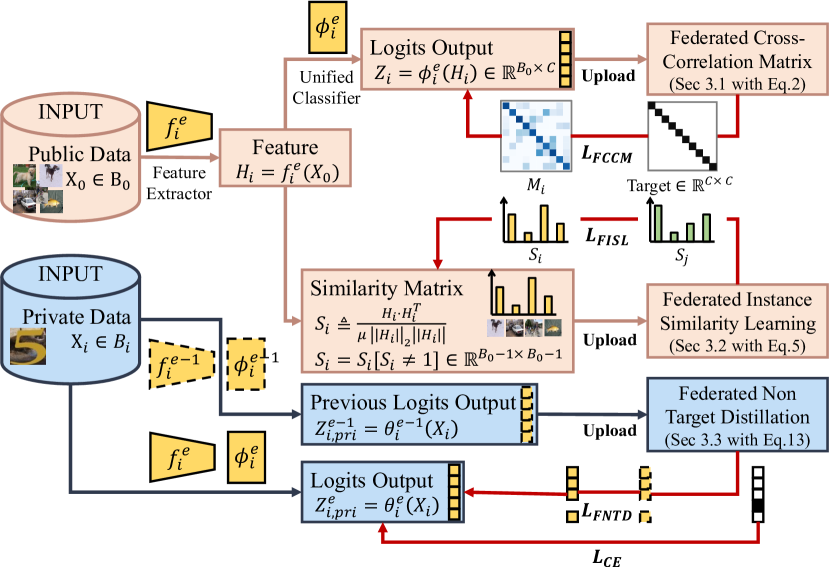
Figure 4: The flow chart of our method. Collaborative updating involves both Federated Cross-Correlation Matrix § 3.1 and Federated Instance Similarity Learning § 3.2 to achieve both feature and logits-level model heterogeneous communication. As for local updating, the Federated Non Target Distillation § 3.3 and Cross Entropy simultaneously regulate local model to balance multiple domain performance.

3.4 Discussion

Conceptual Comparison. We illustrate the proposed method, FCCL+ in Fig. 2 and Algorithm 1 and depict the flowchart in Fig. 4. Our method can be viewed as how to learn more information from others in collaborative updating and how to maintain multiple domains knowledge in local updating. Firstly, we perform communication at both logits and feature levels via FCCM (§ 3.1) and FISL (§ 3.2). Besides, it is applicable to large-scale scenario in federated learning, attributed to that the computation complexity is $\mathcal{O}(K)$. Notably, FCCM and FISL is respectively based on logits output and similarity distribution regardless of the specific model structure. Thus, when participants share same model structure (model homogeneity), ours is still capable. We provide the comparison with state-of-the-art methods under model homogeneity in § 4.4. Secondly, in local updating, FNTD (§ 3.3) disentangles logits knowledge distillation and focuses on transferring inter-domain knowledge, which does not incur heavy computational overhead and does not require complicated hyper-parameter.

Generalization Bound. Driven by the existing related analysis, including single-source domain and multi-domain learning [99, 100, 101, 102, 103] we provide the insight into the generalization bound of heterogeneous federated learning. We denote the global distribution as $\mathcal{D}$, the $i$-th local distribution and its empirical distribution as $\mathcal{D}_{i}$ and $\hat{\mathcal{D}}_{i}$, respectively. In our analysis, we assume a binary classification task, with hypothesis $h$ as a function $h:X\rightarrow\{0,1\}$. The task loss function is formulated as $l(h(x),y)=|\hat{y}-y|$, where $\hat{y}:=h(x)$. Note that $l(\hat{y},y)$ is convex with respect to $\hat{y}$. We denote $\arg\min_{h\in\mathcal{H}}L_{\hat{\mathcal{D}}}(h)$ by $h_{\hat{\mathcal{D}}}$.

Theorem 3.1.

The hypothesis $h\in\mathcal{H}$ learned on $\hat{\mathcal{D}}_{i}$ is denoted by $\smash{h_{\hat{\mathcal{D}}_{i}}}$. The upper bound on the risk of $K$ local models on $\mathcal{D}$ mainly consists of two parts: 1) the empirical risk of the model trained on the global empirical distribution $\hat{\mathcal{D}}=\frac{1}{K}\sum_{i}\hat{\mathcal{D}}_{i}$, and 2) terms dependent on the distribution discrepancy between $\mathcal{D}_{i}$ and $\mathcal{D}$, with the probability $1-\delta$:

$$\small\begin{split}L_{\mathcal{D}}\Big{(}\frac{1}{K}\sum_{i}h_{\hat{\mathcal{D}}_{i}}\Big{)}&\leq L_{\hat{\mathcal{D}}}(h_{\hat{\mathcal{D}}})+\frac{1}{K}\sum_{i}\left(\frac{1}{2}d_{\mathcal{H}\Delta\mathcal{H}}(\mathcal{D}_{i},\mathcal{D})+\lambda_{i}\right)\\ &+\frac{4+\sqrt{\log(\tau_{\mathcal{H}}(2m))}}{\delta/K\sqrt{2m}},\end{split}$$ (15)

where $d_{\mathcal{H}\Delta\mathcal{H}}$ measures the distribution discrepancy between two distributions [104], $m$ is the number of samples per local distribution, $\lambda_{i}$ is the minimum of the combined loss $\mathcal{L}_{\mathcal{D}}(h)\!+\!\mathcal{L}_{\mathcal{D}_{i}}(h),\forall h\in\mathcal{H}$, and $\tau_{\mathcal{H}}$ is the growth function bounded by a polynomial of the VCdim of $\mathcal{H}$.

Proof of Theorem 3.1. We begin with the $L_{\mathcal{D}}\Big{(}\frac{1}{K}\sum_{i}h_{\hat{\mathcal{D}}_{i}}\Big{)}$ risk. By convexity of $l$ and Jensen inequality, we have:

$$\small L_{\mathcal{D}}\Big{(}\frac{1}{K}\sum_{i}h_{\hat{\mathcal{D}}_{i}}\Big{)}\leq\frac{1}{K}\Big{(}\sum_{i}L_{\mathcal{D}}h_{\hat{\mathcal{D}}_{i}}\Big{)}.$$ (16)

Via [102, 105], we transfer from domain $D$ to $D_{i}$ as the following formulation:

$$\small\begin{split}L_{\mathcal{D}}h_{\hat{\mathcal{D}}_{i}}&\leq L_{\mathcal{D}_{i}}(h_{\hat{\mathcal{D}}_{i}})+\frac{1}{2}d_{\mathcal{H}\Delta\mathcal{H}}(\mathcal{D}_{i},\mathcal{D})+\lambda_{i},\\ L_{\mathcal{D}_{i}}(h_{\hat{\mathcal{D}}_{i}})&\leq L_{\hat{\mathcal{D}}_{i}}(h_{\hat{\mathcal{D}}_{i}})+\frac{4+\sqrt{\log(\tau_{\mathcal{H}}(2m))}}{\delta/K\sqrt{2m}}.\end{split}$$ (17)

Based on the definition of ERM: $L_{\hat{\mathcal{D}}_{i}}(h_{\hat{\mathcal{D}}_{i}})\leq L_{\hat{\mathcal{D}}_{i}}(h_{\hat{\mathcal{D}}})$ and the definition: $\hat{\mathcal{D}}=\frac{1}{K}\sum_{i}\hat{\mathcal{D}}_{i}$, we have:

$$\small\frac{1}{K}\sum_{i}L_{\hat{\mathcal{D}}_{i}}(h_{\hat{\mathcal{D}}_{i}})\leq\frac{1}{K}\sum_{i}L_{\hat{\mathcal{D}}_{i}}(h_{\hat{\mathcal{D}}})=L_{\hat{\mathcal{D}}}(h_{\hat{\mathcal{D}}})$$ (18)

Theorem 3.1 reveals that compared to the centralized model on the global empirical distribution, the performance on the global distribution is associated with the discrepancy between local distributions $\mathcal{D}_{i}$ and the global distribution $\mathcal{D}$. The results on different scenarios in Tab. VIII confirm that on the relatively simple scenario, i.e., Digits, ours performs better improvement effect than other scenarios.

Difference with Conference Version. Comparison with FCCL ([1]) (our conference paper), it conducts logits distillation in Eq. 7 with previous model ($\theta^{e-1}$) and pretrained model ($\theta^{*}$) on private data. The local loss is given as:

$$\small\mathcal{L}_{{local}}=\mathcal{L}_{{CE}}+\mathcal{L}_{KD}(\mathcal{T}:\theta^{e-1})+\mathcal{L}_{KD}(\mathcal{T}:\theta^{*}).$$ (19)

Leveraging pre-trained model $\theta^{*}$ to do distillation ($\mathcal{L}_{KD}(\mathcal{T}:\theta^{*})$) is to alleviate the gradient conflict mentioned in LABEL:eq:grad_conflict. However, a well-optimized pretrained model is the prerequisite, which can not be ensured for multiple participants. Therefore, this journal version introduces an improved version, namely FNTD, which simultaneously avoids incompatible optimization objective and gets rid of the assumption of requiring a powerful intra-domain teacher model. By changing the $\mathcal{L}_{KD}(\mathcal{T}:\theta^{e-1})$ to $\mathcal{L}_{{FNTD}}(\mathcal{T}:\theta^{e-1})$, this already avoids the gradient conflict. Hence, the $\mathcal{L}_{KD}(\mathcal{T}:\theta^{*})$ can be deleted in the local updating stage. Therefore, we design the novel and improved local updating objective in Eq. 14, replacing the old one in Eq. 19 as follows:

$$\small\mathcal{L}_{{local}}=\mathcal{L}_{{CE}}+\underbrace{\mathcal{L}_{KD}(\mathcal{T}:\theta^{e-1})}_{\Rightarrow\mathcal{L}_{{FNTD}}(\mathcal{T}:\theta^{e-1})}+\cancel{\mathcal{L}_{KD}(\mathcal{T}:\theta^{*})}.$$ (20)

Communication and Computation Discussion. Regarding the communication aspect, in the model heterogeneous federated learning, different clients hold distinct model architectures, rendering gradient/parameter averaging operations infeasible [106, 8, 19, 107, 21, 108, 109]. Consequently,when dealing with model heterogeneity, leveraging the output signals from the public data presents acts as a practicable communication strategy among heterogeneous clients. Closely related methods, i.e., FedMD [30] and FedDF [32] leverage the logits output to conduct the communication. We further conduct the Federated Instance Similarity Learning module to achieve the feature-level communication for heterogeneous models in order to boost the generalizable performance. Thus, it avoidably brings additional communication cost: instance similarity matrix ($\mathcal{O}{(|B_{0}|^{2})}$), which is dependent on the $|B_{0}|$ scale and does not linearly increase along the network parameter size. We summarize the collaborative communication cost for related methods in Tab. II. In terms of the local computation view, regularization signals act as a crucial character in calibrating the client optimizing direction as data heterogeneity introduces diverse distributions and thus distinct updating objectives. Thus, without regularization signals, clients would optimize towards the local minima and bring catastrophic forgetting on others knowledge, hindering the federated convergence speed. As for FCCL+, it utilizes the previous model to construct distillation to maintain the inter-domain performance, which is also a widely adopted signal to calibrate the local optimization [19, 21, 107, 109]. We provide the local computation cost comparison in the Tab. III.

TABLE II: Communication cost comparison with existing methods from whether supports model heterogeneity (Model Heter.), the selection of communication signals (Comm. Signals), the degree of communication complexity (Comm. Cost). Experimental comparison on Digits inter-domain performance. - denotes these methods are not available for model heterogeneous settings. Refer to § 3.4 and Tab. VIII.

Methods	Comm. Signals	Comm. Cost	Model Heter.	Digits Inter Acc.
FedAvg[8]	Gradient	${|\theta|}$	✗	-
FedProx[19]	Gradient	${|\theta|}$	✗	-
MOON[21]	Gradient	${|\theta|}$	✗	-
FedMD[30]	Logits	${|B_{0}|\!\times\!C}$	✓	26.38
FCCL[1]	Logits	${|B_{0}|\!\times\!C}$	✓	33.51
FCCL+ (Ours)	Logits & Matrix	${|B_{0}|\!\times\!C\!+\!|B_{0}|^{2}}$	✓	50.49

TABLE III: Local computation comparison with existing methods from the resource for parameter space (Para. Space.), the selection of regularization signals, and whether alleviate catastrophic forgetting (Cata. Forg.). All methods default maintain an optimizing model. See details in § 3.4.

Methods	Para. Space	Regularization Signals	Cata. Forg.
Only Model Homogeneous FL
FedAvg[8]	${|\theta|}$	-	✗
FedProx[19]	${2|\theta|}$	Global Model	✓
MOON[21]	${3|\theta|}$	Global & Previous Model	✓
Both Model Homogeneous and Heterogeneous FL
FedMD[30]	${|\theta|}$	-	✗
FCCL[1]	${3|\theta|}$	Previous & Pretrained Model	✓
FCCL+ (Ours)	${2|\theta|}$	Previous Model	✓

TABLE IV: Computation analysis of proposed modules from the increased communication cost (Comm. Cost) and Parameter Space (Para. Space.) aspects. See details in § 3.4.

Module	Comm. Cost	Para. Space	Inter-Domain	Intra-Domain
Collaborative Updating Stage			Digits Mean Acc
FCCM§ 3.1	${|B_{0}|\!\times\!C}$	$|\theta|$	33.51	85.69
FISL§ 3.2	${|B_{0}|^{2}}$	$|\theta|$	37.74	90.14
Local Updating Stage			Digits Mean Acc
FNTD§ 3.3	${|B_{i}|\!\times\!C}$	${2|\theta|}$	50.49	90.57

4 Experiments

4.1 Experimental Setup

Datasets and Models. We extensively evaluate our method on four classification scenarios (i.e., Digits [54, 55, 56, 57], Office Caltech [58], Office31[59] an Office-Home[60]) with three public data (i.e., Cifar-100 [61], Tiny-ImageNet [4] and Fashion-MNIST[62]). For example, for Digits scenario, it includes four domains (i.e., MNIST (M), USPS (U), SVHN (SV) and SYN (SY)) with $10$ categories. Note that for different scenarios, data acquired from different domains present domain shift (data heterogeneity). The example cases in each domain are presented in Fig. 5. As shown in Tab. V, we report the private data scale for each domain calculate and the proportion compared with the complete training data. For these four classification scenarios, participants customize private models that have differentiated backbones and classifiers, (model heterogeneity). For experiments, we randomly set the backbone architecture as ResNet[3], EfficientNet[91], MobileNet[92] and GoogLeNet[110]. We summarize the selected ones for different domains in Tab. VI. As for unified classifier, it maps the embedding feature layer to logits output with 10, 10, 31 and 65 dimensions, which is the classification categories of Digits, Office Caltech, Office31 and Office-Home scenarios, respectively.

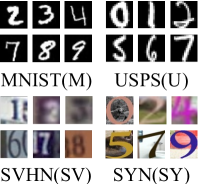
(a) Digits

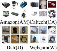
(b) Office Caltech

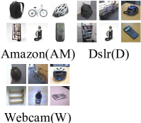
(c) Office31

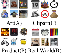
(d) Office-Home

Figure 5: Example cases in Digits[54, 55, 56, 57], Office Caltech [58], Office31 [59] and Office-Home [60] scenarios. See details in § 4.1.

TABLE V: Private data scale in different federated scenarios. Refer to § 4.1.

	Digits				Office Caltech
Scale	M	U	SV	SY	AM	CA	D	W
$N_{i}$	150 (0.25 $\!\%$)	80 (1.10 $\!\%$)	5000 (6.82 $\!\%$)	1800 (18 $\!\%$)	368 (48 $\!\%$)	431 (48 $\!\%$)	60 (48 $\!\%$)	113 (48 $\!\%$)
	Office31				Office-Home
Scale	AM	D	W		A	C	P	R
$N_{i}$	1082 (48 $\!\%$)	192 (48 $\!\%$)	305 (48 $\!\%$)		1400 (82.35 $\!\%$)	2000 (65.57 $\!\%$)	2500 (80.65 $\!\%$)	2000 (65.57 $\!\%$)

TABLE VI: Customized model in four federated scenarios. See details in § 4.1.

Digits				Office Caltech
M	U	SV	SY	AM	CA	D	W
ResNet10	ResNet12	EfficientNet	MobileNet	GoogLeNet	ResNet12	ResNet10	ResNet12
Office31				Office-Home
AM	D	W		A	C	P	R
ResNet10	ResNet12	ResNet10		ResNet18	ResNet34	GoogLeNet	ResNet12

TABLE VII: Hyper-parameters for different federated methods in Digits scenario. Please see more details in § 4.1.

Method	Parameters
FedProx [19]	$\mu$: 0.01
MOON [21]	$\tau$: 0.5, $\mu$: 1
FedProc [107]	$\alpha$: 0.5
FedRS [111]	$\alpha$: 0.5
RHFL [34]	$\alpha$: 0.1, $\beta$: 1.0
FCCL [1]	$\lambda$: 0.0051
FCCL+	$\mu$: 0.002, $\omega$: 3 in § 4.3.2, $\tau$: 3 in § 4.3.3

Evaluation Metric. We report the standard metrics to measure the quality of methods: accuracy, which is defined as the number of samples that are paired divided by the number of samples. Specifically, for evaluation intra and inter-domain performance, we define as follows:

$$\small\mathcal{A}_{i}^{Intra}=\frac{\sum(\texttt{argMax}(f(\theta_{i},X_{i}^{Test}))==Y_{i}^{Test})}{|D_{i}^{Test}|},$$ (21)

$$\small\mathcal{A}_{i}^{Inter}=\sum_{j\neq i}\frac{\sum(\texttt{argMax}(f(\theta_{i},X_{j}^{Test}))==Y_{j}^{Test})}{(K-1)\times|D_{j}^{Test}|}.$$ (22)

For overall performance evaluation, we adopt the average accuracy. Besides, Digits, Office Caltech, Office31 and Office-Home contain 10, 10, 31 and 65 categories. Top-1 and Top-5 accuracy are adopted for the first two and the latter two.

Counterparts. We compare relative federated methods:

- For model heterogeneity based:

• FedMD [NeurIPS’19] [30]: Rely on the related public dataset to conduct distillation operation.

• FedDF [NeurIPS’19] [32]: Ensemble knowledge distillation for robust model fusion via unlabeled data.

• FedMatch [ICLR’21] [112]: Inter-client consistency and disjoint parameters for disjoint learning.

• RHFL [CVPR’22] [34]: Robust noise-tolerant loss for heterogeneous clients under label noise federated learning

• FCCL [CVPR’22] [1]: Align Cross-Correlation with unlabeled data and distill inter-domain knowledge

- For model homogeneity based:

• FedAvg [AISTATS’17] [8]: Average model parameter to realize communication in federated learning

• FedProx [MLSys’20] [19]: Introduce proximal term with the global model parameter via the $\mathcal{L}_{2}$ function

• MOON [CVPR’21] [21]: Pull to the global model and push away the previous local model on feature level

• FedProc [arXiv’21] [107]: Leverage global prototypes to conduct prototype-level contrastive learning

• FedRS [SIGKDD’21] [111]: “Restricted Softmax” limits the update of missing classes’ weights

TABLE VIII: Comparison of inter-domain generalization ($\rightarrow$ ) performance with counterparts on four scenarios with Cifar-100. M$\rightarrow$ means that private data is MNIST and the respective model is tested on all other domains except itself in Eq. 22. AVG denotes the average inter-domain accuracy calculated from each domain. We measure the performance via the mean accuracy of the last three communication epochs. See details in § 4.2. Best in bold and second with underline. These notes are the same to others.

	Digits						Office Caltech
Methods	M$\rightarrow$	U$\rightarrow$	SV$\rightarrow$	SY$\rightarrow$	AVG	$\triangle$	AM$\rightarrow$	CA$\rightarrow$	D$\rightarrow$	W$\rightarrow$	AVG	$\triangle$
BASE	15.29	13.91	39.24	34.30	25.68	-	28.20	32.11	19.99	28.11	27.10	-
FedMD[30]	8.97	12.61	40.89	43.03	26.38	+0.70	21.09	35.13	21.76	30.57	27.13	+0.03
FedDF[32]	13.23	19.29	45.25	43.95	30.43	+4.75	23.87	28.29	16.27	22.82	22.81	-4.29
FedMatch[112]	9.22	14.76	46.28	36.05	26.58	+0.90	19.25	32.21	13.80	22.66	21.98	-5.12
RHFL [34]	19.15	16.72	51.74	48.65	34.06	+8.38	19.11	27.50	16.55	23.83	21.74	-5.36
Our FCCL [1]	20.74	20.60	44.68	48.02	33.51	+7.83	25.16	33.68	17.52	23.81	25.04	-3.07
Our FCCL+	40.13	50.53	48.31	63.00	50.49	+24.81	29.56	36.82	24.02	31.33	30.43	+3.33
	Office31						Office-Home
Methods	AM$\rightarrow$	D$\rightarrow$	W$\rightarrow$		AVG	$\triangle$	A$\rightarrow$	C$\rightarrow$	P$\rightarrow$	R$\rightarrow$	AVG	$\triangle$
BASE	21.08	27.93	34.14		27.72	-	18.89	19.36	21.97	21.02	20.31	-
FedMD[30]	26.26	32.37	40.58		33.07	+5.35	16.85	23.13	28.78	25.01	23.44	+3.13
FedDF[32]	24.74	26.70	35.40		28.96	+1.24	17.38	21.76	25.17	22.97	21.82	+1.51
FedMatch[112]	22.23	31.98	40.15		31.45	+3.73	19.05	25.24	28.73	24.35	24.34	+4.03
RHFL [34]	20.52	20.59	36.32		25.81	-1.91	15.67	20.70	22.02	26.06	21.11	+0.80
Our FCCL [1]	26.69	34.01	39.88		33.52	+5.80	25.55	26.41	30.14	29.41	27.88	+7.49
Our FCCL+	31.87	35.16	44.62		37.21	+9.49	26.67	26.07	25.96	33.02	27.93	+7.62

TABLE IX: Comparison of intra-domain ($\hookleftarrow$) performance with counterparts on four scenarios with Cifar-100. The intra-domain accuracy metric ($\hookleftarrow$) in Eq. 21 is evaluated on respective testing data. See details in § 4.2.

	Digits						Office Caltech
Methods	M$\hookleftarrow$	U$\hookleftarrow$	SV$\hookleftarrow$	SY$\hookleftarrow$	AVG	$\triangle$	AM$\hookleftarrow$	CA$\hookleftarrow$	D$\hookleftarrow$	W$\hookleftarrow$	AVG	$\triangle$
BASE	70.20	74.19	74.57	73.60	73.14	-	74.11	61.35	75.16	78.31	72.23	-
FedMD[30]	77.30	80.05	77.73	87.72	80.70	+7.56	71.78	57.29	68.37	72.20	67.41	-4.82
FedDF[32]	82.95	78.84	78.46	91.30	83.38	+10.24	70.01	56.49	65.18	64.86	64.13	-8.10
FedMatch[112]	82.69	78.31	79.79	89.23	82.69	+9.55	73.38	60.25	68.58	73.56	68.94	-3.29
RHFL [34]	86.69	80.39	88.44	97.90	88.35	+15.21	73.35	58.92	70.91	74.47	69.41	-2.82
Our FCCL [1]	88.84	84.42	78.55	91.23	85.69	+12.55	75.09	60.46	74.95	73.56	71.01	-1.22
Our FCCL+	90.54	86.92	87.11	97.72	90.57	+17.43	75.26	59.90	75.80	75.48	71.60	-0.63
	Office31						Office-Home
Methods	AM$\hookleftarrow$	D$\hookleftarrow$	W$\hookleftarrow$		AVG	$\triangle$	A$\hookleftarrow$	C$\hookleftarrow$	P$\hookleftarrow$	R$\hookleftarrow$	AVG	$\triangle$
BASE	72.95	77.31	80.88		77.04	-	65.27	60.50	74.68	54.28	63.68	-
FedMD[30]	71.39	76.24	80.13		75.92	-1.12	66.17	60.63	76.35	56.60	64.93	+1.25
FedDF[32]	72.25	74.50	80.34		75.69	-1.35	66.10	60.44	75.70	55.98	64.55	+0.87
FedMatch[112]	71.08	76.04	80.92		76.01	-1.03	81.50	65.40	79.81	65.06	72.94	+9.26
RHFL [34]	70.98	73.90	78.87		74.58	-2.46	56.68	73.79	76.29	63.63	67.59	+3.91
Our FCCL [1]	72.37	78.44	81.26		77.35	+0.31	81.51	65.42	79.84	65.16	72.98	+9.30
Our FCCL+	72.92	78.61	81.26		77.59	+0.55	69.74	74.65	78.02	69.02	72.85	+9.17

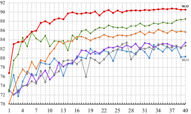
(a) Digits

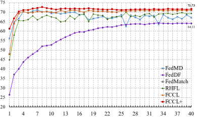
(b) Office Caltech

Figure 6: Comparison of average intra-domain accuracy during federated learning process with counterparts in Digits and Office Caltech scenarios with Cifar-100. The horizontal and vertical coordinates represent the communication epoch and intra-domain accuracy. We mark the best and worst performance of the last communication epoch. Refer to § 4.2 for details.

Implement Details. For a fair comparison, we follow [32, 21, 1, 34]. The clients scale are dependent on the experimental scenario. For example, in digits, there are four clients. Models are trained via Adam optimizer [113] with batch size of $512$ and $256$ in collaborative updating and local updating. The learning rate is consistent $0.001$ in these two process for all approaches. We set the hyper-parameter $\lambda=0.0051$ like [45] and $\mu=0.02$ in [114]). We further conduct hyper-parameter analysis of $\omega$ and $\tau$ in Tab. XIV and Fig. 10. The number of unlabeled public data is $5000$ for different scenarios. Besides, we analyze the effect of strong and weak data augmentations on public data for FISL in § 4.3.2, and follow the data augmentation in [82, 115] to construct strong data augmentation We list these data augmentations following the PyTorch notations:

• RandomResizedCrop: Crop with the scale of $(0.2,1.)$. and images are resized to $32\times 32$.

• RandomHorizontalFlip: The given image is horizontally flipped randomly with a given probability $p=0.5$.

• ColorJitter: We randomly change the brightness, contrast, saturation and hue of images with value as $(0.4,0.4,0.4,$ $0.1)$ and set the probability as $0.8$.

• RandomGrayscale: Randomly convert image to grayscale with a probability of $p=0.2$.

Besides, for the weak data augmentation, we only maintain RandomResizedCrop and RandomHorizontalFlip strategies for public data. See detail in § 4.1 and relative analysis in § 4.3.2. We follow the data augmentation strategy in [82, 115] to construct strong data augmentation. We list these data augmentations following the PyTorch notations:

• RandomResizedCrop: We crop Cifar-100, Tiny-ImageNet and with the scale of $(0.2,1.)$. The cropped images are resized to $32\times 32$, $32\times 32$ for these two public data.

• RandomHorizontalFlip: The given image is horizontally flipped randomly with a given probability $p=0.5$.

• ColorJitter: We randomly change the brightness, contrast, saturation and hue of images with value as $(0.4,0.4,0.4,$ $0.1)$ and set the probability as $0.8$.

• RandomGrayscale: Randomly convert image to grayscale with a probability of $p=0.2$.

For pre-processing, we resize all input images into $32\times 32$ with three channels for compatibility. We do the communication for $E\!=\!40$ epochs, where all approaches have little or no accuracy gain with more rounds. For BASE, models are optimized on private data for $50$ epochs.

4.2 Comparison with SOTA Methods

We comprehensively examine the proposed method with state-of-the-art methods on four image classification tasks, i.e., Digits [54, 55, 56, 57], Office Caltech [58], Office31 [59] and Office-Home [60]) with three public data (i.e., Cifar-100 [61], Tiny-ImageNet [4] and Fashion-MNIST [62]).

Inter-domain Generalization Analysis. We summarize the results of inter-domain accuracy by the end of federated learning in Tab. VIII. As shown in the table, it clearly depicts that under domain shift, BASE presents worst in these two tasks, demonstrating the benefits of federated learning. FCCL+ consistently outperforms all other counterparts on different scenarios. For example, in Digits scenario, FCCL+ outperforms the best counterparts by $19.39\%$ on MNIST, which is calculated through the average testing accuracy for respective model on USPS, SYN and SVHN testing data. We conduct experiments in Tab. XII with the Tiny-ImageNet datasets on the Digits scenario, and ours achieves consistently superior performance.

Intra-domain Discrimination Analysis. To demonstrate the effectiveness of alleviating catastrophic forgetting on intra-domain, we observe that our method almost outperforms the compared methods by a large margin along the federated learning process in Fig. 6. We further report the final intra-domain accuracy in Tab. IX. Although BASE achieves relatively competitive intra-domain performance, the reason is that it purely optimizes on the local data without collaborating with others. However, the lack of collaboration hinders the generalization of BASE on inter-domain evaluation, where the data distributions may be significantly distinct from the local data. FCCL+ suffers less periodic performance shock and is not prone to overfitting to local data distribution. The Tab. VIII and Tab. IX illustrate that FCCL+ is capable of balancing multiple domain knowledge and effectively alleviates the catastrophic forgetting problem.

TABLE X: Ablation study of key components of our proposed method in Digits and Office31 scenarios with Cifar-100. Both inter-domain generalization ($\rightarrow$) and intra-domain discriminability ($\hookleftarrow$) accuracies are reported. Please see § 4.3 for details.

			Digits						Office31
FCCM	FISL	FNTD	M$\rightarrow$	U$\rightarrow$	SV$\rightarrow$	SY$\rightarrow$	AVG	$\triangle$	AM$\rightarrow$	D$\rightarrow$	W$\rightarrow$	AVG	$\triangle$
			15.29	13.91	39.24	34.30	26.68	-	21.08	27.93	34.14	27.72	-
✓			20.74	20.60	44.68	48.02	33.51	+6.83	26.69	34.01	39.88	33.52	+5.80
	✓		25.59	24.75	47.53	53.12	37.74	+11.06	20.02	28.04	36.51	28.19	+0.47
✓	✓		30.97	25.90	51.12	53.84	40.45	+13.77	26.08	31.64	38.74	32.15	+4.43
✓	✓	✓	40.13	50.53	48.31	63.00	50.49	+23.81	30.95	32.77	45.38	36.36	+8.64
			Digits						Office31
FCCM	FISL	FNTD	M$\hookleftarrow$	U$\hookleftarrow$	SV$\hookleftarrow$	SY$\hookleftarrow$	AVG	$\triangle$	AM$\hookleftarrow$	D$\hookleftarrow$	W$\hookleftarrow$	AVG	$\triangle$
			70.20	74.19	74.57	73.60	73.14	-	72.95	77.31	80.88	77.04	-
✓			88.84	84.42	78.55	91.23	85.69	+12.55	72.37	78.44	81.26	77.35	+0.31
	✓		88.36	86.68	88.42	97.12	90.14	+17.00	72.32	77.91	81.59	77.27	+0.23
✓	✓		88.27	87.81	88.04	97.08	90.30	+17.16	72.79	77.91	81.81	77.50	+0.46
✓	✓	✓	90.54	86.92	87.11	97.72	90.57	+17.43	72.92	78.61	81.26	77.59	+0.51

TABLE XI: Analysis of FCCM with different hyper-parameter $\lambda$ in Eq. 2 on the Office31 scenario for the inter- and intra- overall performance. See details in § 4.3.3.

Inter-domain					Intra-domain
0.002	0.0051	0.01	0.05	0.1	0.002	0.0051	0.01	0.05	0.1
33.09	33.52	32.89	32.41	32.51	77.54	77.35	77.60	77.00	77.53

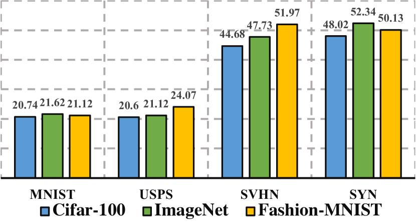
Public Data	AVG
Cifar-100	33.51
Tiny-ImageNet	35.70
Fashion-MNIST	36.82

Figure 7: Ablation study on FCCM (§ 3.1) with different public data for inter-domain generalization ($\rightarrow$) on each domain (Histogram) and overall performance (Table) in Digits task. See details in § 4.3.1.

TABLE XII: Comparison of inter-domain generalization ($\rightarrow$ ) performance and intra-domain discriminability ($\hookleftarrow$) with counterparts on Digits scenario with Tiny-ImageNet. ”/” means optimization dilemma, i.e., FedDF with Tiny-ImageNet. Refer to § 4.2.

	Tiny-ImageNet
Methods	M$\rightarrow$	U$\rightarrow$	SV$\rightarrow$	SY$\rightarrow$	AVG
BASE	15.29	13.91	39.24	34.30	25.68
FedMD[30]	18.50	13.26	51.23	52.06	33.76
FedMatch[112]	11.77	11.49	46.65	46.33	29.06
RHFL [34]	16.14	14.05	54.26	47.57	33.00
Our FCCL [1]	31.84	31.03	46.81	52.75	40.60
Our FCCL+	30.15	48.33	50.88	61.84	47.80
	Tiny-ImageNet
Methods	M$\hookleftarrow$	U$\hookleftarrow$	SV$\hookleftarrow$	SY$\hookleftarrow$	AVG
BASE	70.20	74.19	74.57	73.60	73.14
FedMD[30]	84.64	34.31	87.35	98.10	76.10
FedMatch[112]	86.60	49.98	87.45	97.58	80.40
RHFL [34]	75.06	55.19	88.49	97.23	78.99
Our FCCL [1]	87.34	85.03	87.89	93.98	88.56
Our FCCL+	91.32	84.70	87.41	98.08	90.37

4.3 Diagnostic Experiments

For thoroughly assessing the efficacy of essential components of our approach, we perform an ablation study on Digits and Office31 to investigate the effect of each essential component: Federated Cross-Correlation Matrix (FCCM § 3.1), Federated Instance Similarity Learning (FISL § 3.2) and Federated Non Target Distillation (FNTD § 3.3). We firstly give a quantitative result of inter- and intra-domains performance on these three components in Tab. X. For the local updating phase without FNTD module, experiments remain same optimization objective as our conference version in Eq. 19 because FCCM and FISL are designed for how to better learn from others in collaborative updating, rather than alleviate catastrophic forgetting. The first row refers to a baseline that only respectively trains on private data. Three crucial conclusions can be drawn. First, FCCM leads to significant performance improvements against the baseline across all the metrics on both scenarios. This evidences that our cross-correlation learning strategy is able to produce generalizable performance. Second, we also observe compelling gains by incorporating FISL into the baseline. This proves the importance of feature-level communication. Besides, combining FCCM and FISL achieves better performance, which supports our motivation of exploiting joint logits and feature levels communication rather than only focusing on logits output in model heterogeneity. Third, our full method leads to the best performance, by further leveraging FNTD in local updating phase, which suggests that these modules are complementary to each other, and confirms the effectiveness of our whole design. Besides, FCCL+ maintains the robustness with diverse architecture selection, as illustrated in Tab. XVIII.

(a) Epoch 1

(b) Epoch 5

(c) Epoch 10

(d) Epoch 20

(e) Epoch 40

Figure 8: Cross-correlation matrix visualization for different domains in Digits scenario with Cifar-100. The matrix is $10\times 10$. We visualize the cross-correlation matrix ($\mathcal{M}_{i}$ in Eq. 1) with others on unlabeled public data (Left Column). Besides, for each domain, we represent the $\mathcal{M}_{i}$ with others on respective private data (Right Column). The darker the color, the closer the $\mathcal{M}_{i}^{uv}$ is to $1$. Best viewed in color. See details in § 4.3.1.

4.3.1 Federated Cross-Correlation Matrix

To prove Federated Cross-Correlation Matrix (FCCM) robustness and stability, we next evaluate the performance on different public data (i.e., Cifar-100, Tiny-ImageNet and Fashion-MNIST). The Fig. 7 suggests that Federated Cross-Correlation Matrix achieves consistent performance in each domain. Moreover, it can be seen that it is more effective by the use of public data with rich categories (Tiny-ImageNet) or simple details (Fashion-MNIST). Besides, the Fig. 8 presents that FCCM achieves similar logits output among participants and minimizes the redundancy within the logits output, confirming that FCCM successfully enforces the correlation of same dimensions and decorrelation of different dimensions on both public and private data.

TABLE XIII: Analysis of public data diversity and data augmentation effect for FISL (§ 3.2) in Digits and Office31 scenarios. See details in § 4.3.2.

	Digits					Office31
Aug	M$\rightarrow$	U$\rightarrow$	SV$\rightarrow$	SY$\rightarrow$	AVG	AM$\rightarrow$	D$\rightarrow$	W$\rightarrow$	AVG
Fashion-MNIST
weak	23.84	20.03	46.86	49.28	35.00	20.40	29.59	35.87	28.62
strong	24.45	21.91	46.38	47.09	34.95	19.00	28.37	35.42	27.59
Cifar-100
weak	25.59	24.75	47.53	53.12	37.74	20.02	28.04	36.51	28.19
strong	26.36	21.28	50.03	50.99	37.16	20.83	28.18	36.11	28.37
Tiny-ImageNet
weak	27.60	27.08	45.66	51.94	38.07	21.05	28.36	34.81	28.07
strong	25.60	29.95	40.41	50.83	36.69	21.12	30.43	34.14	28.56

TABLE XIV: Analysis of weighting hyper-parameter, $\omega$ for $\mathcal{L}_{{FISL}{}}$ in $\mathcal{L}_{colla}$ (Eq. 6) in Digits and Office31 with Cifar-100. See details in § 4.3.2.

$\omega$	Digits					Office31
Eq. 6	M$\rightarrow$	U$\rightarrow$	SV$\rightarrow$	SY$\rightarrow$	AVG	AM$\rightarrow$	D$\rightarrow$	W$\rightarrow$	AVG
$1$	25.54	21.95	50.22	52.08	37.44	25.35	31.22	37.57	31.38
$2$	28.69	23.95	50.88	51.28	38.70	26.88	31.16	37.70	31.91
$3$	30.97	25.90	51.12	53.84	40.45	26.08	31.64	38.74	32.15
$4$	27.01	24.12	52.08	54.70	39.47	27.25	29.24	37.86	31.45

TABLE XV: Comparison with state-of-the-art homogeneous federated learning methods under model homogeneity in Digits and Office31 scenarios with Cifar-100. Both intra-domain discriminability ($\hookleftarrow$) and inter-domain generalization ($\rightarrow$) accuracies are reported. See details in § 4.4.

	Digits						Office31
Methods	M$\rightarrow$	U$\rightarrow$	SV$\rightarrow$	SY$\rightarrow$	AVG	$\triangle$	AM$\rightarrow$	D$\rightarrow$	W$\rightarrow$	AVG	$\triangle$
BASE	14.36	13.82	50.75	46.83	31.44	-	22.00	32.50	36.16	30.22	-
FedAvg [30]	74.55	77.42	66.36	83.86	75.54	+44.10	60.06	54.69	59.50	58.08	+27.86
FedProx [19]	87.61	89.49	85.71	84.40	86.80	+55.36	64.74	61.32	69.81	65.29	+35.07
FedMD [30]	78.19	81.29	66.53	80.81	76.70	+45.26	66.09	59.05	66.08	63.74	+33.52
FedDF [32]	77.61	80.90	68.93	83.92	77.84	+46.40	55.82	44.30	60.30	53.47	+23.25
MOON ($\tau=5$) [21]	57.55	67.65	62.95	76.52	66.16	+34.72	63.32	58.72	64.42	62.15	+31.93
MOON ($\tau=1$) [21]	76.81	78.10	72.99	83.50	77.85	+46.41	64.76	62.20	67.53	64.83	+34.61
FedProc [107]	72.05	74.12	62.57	78.34	71.77	+40.33	37.61	45.20	55.86	46.22	+ 16.00
FedRS [111]	55.28	65.80	61.59	73.23	63.97	+32.53	46.77	47.75	54.56	49.69	+19.47
Our FCCL [1]	77.18	79.11	68.96	85.26	77.62	+46.18	55.39	46.16	61.60	54.38	+24.16
Our FCCL+	78.99	80.54	72.15	85.38	79.26	+47.82	72.39	55.00	71.49	66.69	+36.47
	Digits						Office31
Methods	M$\hookleftarrow$	U$\hookleftarrow$	SV$\hookleftarrow$	SY$\hookleftarrow$	AVG	$\triangle$	AM$\hookleftarrow$	D$\hookleftarrow$	W$\hookleftarrow$	AVG	$\triangle$
BASE	82.09	77.15	90.10	98.08	86.85	-	71.58	73.63	78.07	74.42	-
FedAvg [30]	92.50	91.48	90.98	85.27	90.05	+3.20	71.25	77.58	78.20	75.67	+1.25
FedProx [19]	92.44	90.36	92.08	96.20	92.77	+5.92	71.58	76.24	80.71	76.17	+1.75
FedMD [30]	90.55	88.82	90.79	88.17	89.58	+2.73	70.96	78.24	78.58	75.92	+1.50
FedDF [32]	91.08	89.70	90.81	87.51	89.77	+2.92	70.95	77.84	78.99	75.92	+1.50
MOON ($\tau=5$)[21]	87.58	84.46	87.70	70.28	82.50	-4.35	67.51	70.68	74.01	70.73	-3.69
MOON ($\tau=1$) [21]	91.63	89.02	90.91	77.27	87.20	+1.35	69.00	74.90	76.61	73.50	-0.92
FedProc [107]	85.91	83.53	89.01	76.62	83.76	-3.09	69.38	75.24	78.95	74.52	+0.10
FedRS [111]	82.27	85.91	86.79	71.65	81.65	-5.20	70.86	75.63	79.22	75.23	+0.81
Our FCCL [1]	90.71	90.61	90.92	83.40	88.91	+2.06	72.34	77.31	81.68	77.11	+2.69
Our FCCL+	93.74	90.78	90.71	80.68	88.97	+2.12	71.65	78.58	82.73	77.65	+3.23

TABLE XVI: Compare average inter-domain generalization performance of FNTD with EWC [116] in different hyper-parameter: $\lambda$ on Digits (Left) and Office31 (Right) scenarios. See details in § 4.3.3.

	EWC ($\lambda$)					EWC ($\lambda$)
Ours	0.01	0.1	0.7	1.0	Ours	0.01	0.1	0.7	1.0
50.49	28.50	28.38	29.08	28.70	37.21	29.58	28.59	29.04	29.18

TABLE XVII: Ablation of incorporating KD with FNTD in Digits and Office31 scenarios. This ratio represents the proportion of KD in the local training process. “0” means purely leveraging FNTD in the local updating. Please see details in § 4.3.3.

	Digits
w KD	M$\rightarrow$	U$\rightarrow$	SV$\rightarrow$	SY$\rightarrow$	AVG	M$\hookleftarrow$	U$\hookleftarrow$	SV$\hookleftarrow$	SY$\hookleftarrow$	AVG
30%	24.25	25.39	45.55	56.54	37.93	87.79	85.10	86.70	97.12	89.17
10%	26.66	33.61	48.70	56.56	41.38	89.54	88.59	87.32	97.07	90.63
0	40.13	50.53	48.31	63.00	50.49	90.54	86.92	87.11	97.72	90.57

TABLE XVIII: Ablation of different network selection in the Digits scenario with Cifar-100 dataset. The default architecture is in Tab. VI. See § 4.3.

	Digits
Methods	M$\rightarrow$	U$\rightarrow$	SV$\rightarrow$	SY$\rightarrow$	AVG	M$\hookleftarrow$	U$\hookleftarrow$	SV$\hookleftarrow$	SY$\hookleftarrow$	AVG
M: ResNet10 U: ResNet12 SV: EfficientNet SY: SimpleCNN
FedMD	20.83	16.92	48.73	31.45	29.48	85.00	67.02	86.49	87.38	81.47
FCCL	22.09	16.71	50.49	37.63	31.73	86.98	82.33	88.26	84.12	85.42
FCCL+	37.13	45.97	49.12	52.99	46.30	91.79	88.24	87.57	86.17	88.44
M: ResNet18 U: ResNet12 SV: EfficientNet SY: MobileNet
FedMD	19.27	14.58	43.74	46.18	30.94	90.20	55.12	87.16	97.80	82.57
FCCL	24.74	16.57	50.63	49.35	35.32	89.98	83.76	87.22	97.28	89.56
FCCL+	56.71	45.07	53.03	61.05	53.96	93.23	87.31	87.94	96.92	91.35

TABLE XIX: Catastrophic forgetting effect with different local epochs in the Digits scenario with Cifar-100 dataset. w/o FNTD denotes without FNTD module in Eq. 14. Refer to § 4.3.3 for details.

Local	w/o FNTD					w/ FNTD
Epoch	M$\rightarrow$	U$\rightarrow$	SV$\rightarrow$	SY$\rightarrow$	AVG	M$\rightarrow$	U$\rightarrow$	SV$\rightarrow$	SY$\rightarrow$	AVG
10	18.56	15.54	45.71	47.37	31.79	21.81	16.09	48.54	49.78	34.05
20	17.50	15.35	48.32	54.67	33.96	40.13	50.53	48.31	63.00	50.49
30	17.15	16.23	47.93	50.25	32.89	33.35	40.69	49.82	57.49	45.33

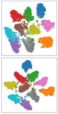
(a) M$\rightarrow$M

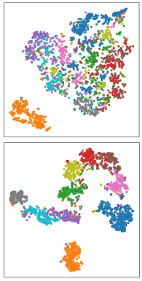
(b) M$\rightarrow$U

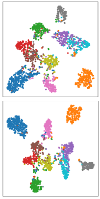
(c) U$\rightarrow$U

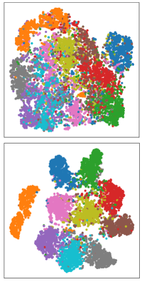
(d) U$\rightarrow$M

$\mathcal{T}$	Digits
Eq. 13	M$\rightarrow$	U$\rightarrow$	SV$\rightarrow$	SY$\rightarrow$	AVG
$\theta^{e}$	16.08	20.25	34.75	45.95	29.25
$\theta^{e-1}$	40.13	50.53	48.31	63.00	50.49
$\mathcal{T}$	Digits
Eq. 13	M$\hookleftarrow$	U$\hookleftarrow$	SV$\hookleftarrow$	SY$\hookleftarrow$	AVG
$\theta^{e}$	88.31	73.11	82.95	95.58	84.98
$\theta^{e-1}$	90.54	86.92	87.11	97.72	90.57

Figure 9: Analysis of teacher, $\mathcal{T}$ in FNTD (Eq. 13) for Digits scenario with Cifar-100. We visualize the learned feature on intra-domain (i.e., M $\rightarrow$ M) and inter-domain (i.e., M $\rightarrow$ U) with $\theta^{e-1}$ (Bottom Row) and $\theta^{e}$ (Top Row). Features are colored based on labels. Refer to § 4.3.3.

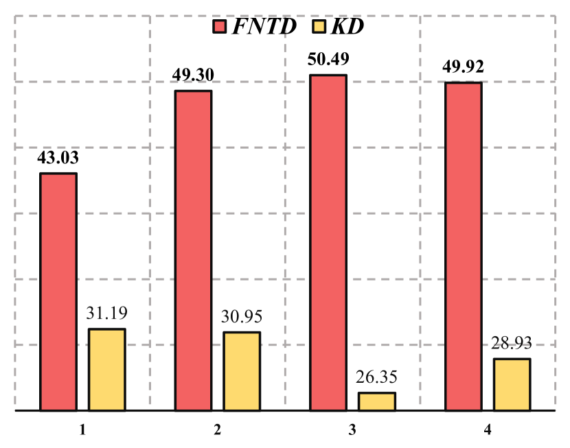
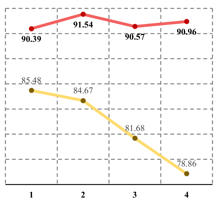
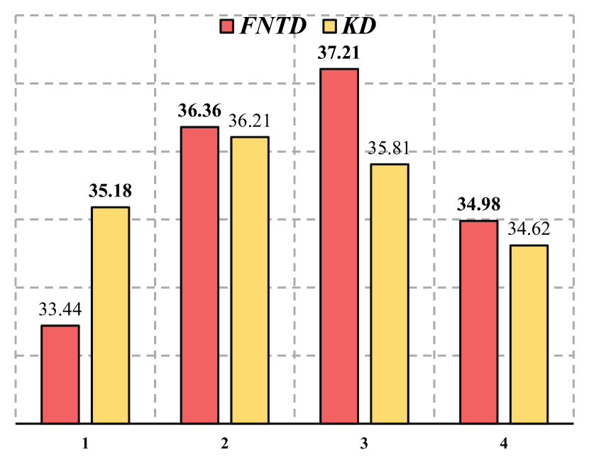
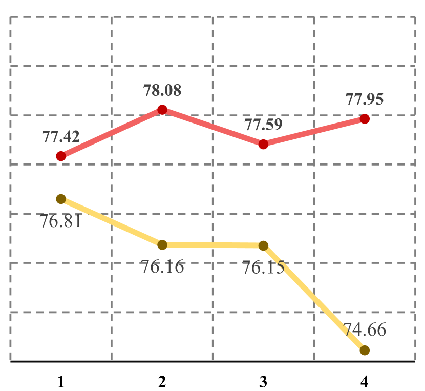
Figure 10: Comparison of FNTD (Eq. 13) and KD (Eq. 7) with different temperature hyper-parameter, $\tau$ in Eq. 8 for inter-domain performance (Histogram) and intra-domain performance (Line) in Digits and Office31 scenarios with Cifar-100. See details in § 4.3.3.

4.3.2 Federated Instance Similarity Learning

We next examine the design of our Federated Instance Similarity Learning (FISL). FISL aims to reach similarity distribution alignment on unlabeled public data. Thus, we analyze the impact of diversity and augmentation on public data in Tab. XIII. The results reveal that for simple scenarios, i.e., Digits (10 categories), leveraging weak augmentation is more beneficial, which is contrary for complicated scenarios i.e., Office31 (31 categories). Besides, different scenarios would benefit from the diversity of public data. Specifically, in Digits scenario, the average inter-domain performance increase from $37.74\%$ to $38.07\%$ when public data change from Cifar-100 to Tiny-ImageNet with weak data augmentation. The details of weak and strong data augmentation are listed in § 4.1. It shows that the proposed module FISL is robust under different data augmentations and shows comparable performance under different scenarios. Then, in Tab. XIV, we analyze the impact of the weighting hyper-parameter, $\omega$ for $\mathcal{L}_{{FISL}{}}$ in $\mathcal{L}_{colla}$ (Eq. 6). As seen, the inter-domain performance progressively improves as $\omega$ is increased, and the gain becomes marginal when $\omega\!=\!3$. Hence, we select the $\omega\!=\!3$ by default in different scenarios.

4.3.3 Federated Non Target Distillation

As shown in Tab. XIX, without inter-domain knowledge regularization, local model would present serious catastrophic forgetting phenomenon on the inter-domain performance, demonstrating the importance of incorporating inter-domain knowledge in the local updating stage. We then investigate the effectiveness of Federated Non Target Distillation (FNTD). In Fig. 10, the ✗ refers to the typical knowledge distillation (KD) in Eq. 7. Our FNTD outperforms the typical KD by avoiding optimization conflict. The gains become larger in the relatively easy scenario, i.e., Digits because the objective is easier contradictory under the supervision of private data label information and more ’confident’ previous model. Besides, we assess the impact of the temperature hyper-parameter, $\tau$ (Eq. 8) in $\mathcal{L}_{{FNTD}{}}$ (Eq. 13). We find that the suitable temperature is $3$. We believe this happens because a small temperature obstacles more information of non-targets to be distilled and a large temperature blindly softens logits distribution, which falls back to a uniform distribution and is not informative, corroborating relevant observations reported in [36, 52, 117]. Hence, we apply temperature $\tau\!=\!3$ by default. Finally, we study the selection of the teacher model in FNTD (Eq. 13). We give a comparison of using different models: $\theta^{e-1}$ (after local updating) and $\theta^{e}$ (after collaborative updating) as teacher model in local updating. We draw t-SNE [118] visualization of data embeddings on the testing data and inter-domain performance by the end of federated learning in Fig. 9. This proves that $\theta^{e-1}$ is better than $\theta^{e}$ to maintain inter- and intra-domains knowledge in local updating simultaneously. We further replace the proposed module FNTD with the EWC penalty [116] in Tab. XVI. It reveals that ours performs better than the existing relative methods in handling the catastrophic forgetting problem. Besides, we consider investigating the effectiveness of target distillation in the first half of local updating rounds in Tab. XVII. It reveals that purely leveraging FNTD achieves better performance. We argue that the confidence in the target class is uncontrollable and thus results in the underlying optimization conflict. Besides, defining the proportion of utilization rounds would bring additional hyper-parameter.

4.4 Model Homogeneity Analysis

We further compare FCCL+ with other methods under model homogeneous setting. We set the global shared model as ResNet12 and add the model parameter averaging operation between collaborative updating and local updating. The Tab. XV presents both inter- and intra-domains performance on Digits and Office31 scenarios with Cifar-100. Although FedProx achieve competitive performance in certain simple scenarios, i.e., Digits, it requires parameter element-wise regularization, which incurs heavy computation cost and limits the generalization ability [119] in the challenging scenarios with the large domain shift such as Office31. In contrast, our method relies on the logits output, which remains a static target without recycle updating requirements and does not largely increase the computational burden with different network backbones. Therefore, considering the computation cost and the underlying large domain shift in heterogeneous federated learning scenarios, FCCL+ emerges as a superior candidate compared to FedProx.

5 Conclusion

In this paper, we present FCCL+, a novel and effective solution for heterogeneous federated learning. FCCL+ exploit both logits and feature levels knowledge communication by constructing cross-correlation matrix and measuring instance similarity distribution on unlabeled public data, effectively overcoming communication barrier and acquiring generalizable ability in heterogeneous federated learning. Besides, for alleviating catastrophic forgetting problem, we disentangle typical knowledge distillation to avoid optimization conflict and better preserve inter-domain knowledge. Moreover, we maintain the supervision of label signal to provide strong intra-domain constraint, boosting both inter- and intra-domains performance. We experimentally show that FCCL+ performs favorably with many existing related methods on four different scenarios. We wish this work to pave the way for future research on heterogeneous federated learning as it is fully reproducible and includes:

• FCCL+, a strong baseline that outperforms others while maintaining limited communication burden on server and friendly computation cost for participants.

• A clear and extensive benchmark comparison of the state-of-the-art on multiple domain shift scenarios.

References

- [1] W. Huang, M. Ye, and B. Du, “Learn from others and be yourself in heterogeneous federated learning,” in CVPR, 2022.
- [2] A. Krizhevsky, I. Sutskever, and G. E. Hinton, “Imagenet classification with deep convolutional neural networks,” in NeurIPS, 2012, pp. 1097–1105.
- [3] K. He, X. Zhang, S. Ren, and J. Sun, “Deep residual learning for image recognition,” in CVPR, 2016, pp. 770–778.
- [4] O. Russakovsky, J. Deng, H. Su, J. Krause, S. Satheesh, S. Ma, Z. Huang, A. Karpathy, A. Khosla, M. Bernstein, A. C. Berg, and L. Fei-Fei, “Imagenet large scale visual recognition challenge,” IJCV, pp. 211–252, 2015.
- [5] T.-Y. Lin, M. Maire, S. Belongie, J. Hays, P. Perona, D. Ramanan, P. Dollár, and C. L. Zitnick, “Microsoft coco: Common objects in context,” in ECCV, 2014, pp. 740–755.
- [6] H. Li, M. Ye, and B. Du, “Weperson: Learning a generalized re-identification model from all-weather virtual data,” in ACM MM, 2021.
- [7] P. Voigt and A. Von dem Bussche, “The eu general data protection regulation (gdpr),” A Practical Guide, 1st Ed., Cham: Springer International Publishing, p. 3152676, 2017.
- [8] B. McMahan, E. Moore, D. Ramage, S. Hampson, and B. A. y Arcas, “Communication-efficient learning of deep networks from decentralized data,” in AISTATS, 2017, pp. 1273–1282.
- [9] Q. Yang, Y. Liu, T. Chen, and Y. Tong, “Federated machine learning: Concept and applications,” ACM TIST, pp. 1–19, 2019.
- [10] J. Sun, T. Chen, G. B. Giannakis, Q. Yang, and Z. Yang, “Lazily aggregated quantized gradient innovation for communication-efficient federated learning,” IEEE PAMI, vol. 44, no. 4, pp. 2031–2044, 2020.
- [11] S. Hong and J. Chae, “Communication-efficient randomized algorithm for multi-kernel online federated learning,” IEEE PAMI, vol. 44, no. 12, pp. 9872–9886, 2021.
- [12] A. Hard, K. Rao, R. Mathews, S. Ramaswamy, F. Beaufays, S. Augenstein, H. Eichner, C. Kiddon, and D. Ramage, “Federated learning for mobile keyboard prediction,” arXiv preprint arXiv:1811.03604, 2018.
- [13] Q. Liu, C. Chen, J. Qin, Q. Dou, and P.-A. Heng, “Feddg: Federated domain generalization on medical image segmentation via episodic learning in continuous frequency space,” in CVPR, 2021, pp. 1013–1023.
- [14] X. Guo, P. Xing, S. Feng, B. Li, and C. Miao, “Federated learning with diversified preference for humor recognition,” in IJCAI Workshop, 2020.
- [15] P. Kairouz, H. B. McMahan, B. Avent, A. Bellet, M. Bennis, A. N. Bhagoji, K. Bonawitz, Z. Charles, G. Cormode, R. Cummings et al., “Advances and open problems in federated learning,” arXiv preprint arXiv:1912.04977, 2019.
- [16] Q. Li, Y. Diao, Q. Chen, and B. He, “Federated learning on non-iid data silos: An experimental study,” IEEE TKDE, 2022.
- [17] M. Ye, X. Fang, B. Du, P. C. Yuen, and D. Tao, “Heterogeneous federated learning: State-of-the-art and research challenges,” CSUR, 2023.
- [18] A. Z. Tan, H. Yu, L. Cui, and Q. Yang, “Towards personalized federated learning,” IEEE TNNLS, 2022.
- [19] T. Li, A. K. Sahu, M. Zaheer, M. Sanjabi, A. Talwalkar, and V. Smith, “Federated optimization in heterogeneous networks,” in MLSys, 2020.
- [20] N. Shoham, T. Avidor, A. Keren, N. Israel, D. Benditkis, L. Mor-Yosef, and I. Zeitak, “Overcoming forgetting in federated learning on non-iid data,” in NeurIPS Workshop, 2019.
- [21] Q. Li, B. He, and D. Song, “Model-contrastive federated learning,” in CVPR, 2021, pp. 10 713–10 722.
- [22] J. Quiñonero-Candela, M. Sugiyama, N. D. Lawrence, and A. Schwaighofer, Dataset Shift in Machine Learning. Mit Press, 2009.
- [23] S. J. Pan and Q. Yang, “A survey on transfer learning,” IEEE TKDE, pp. 1345–1359, 2009.
- [24] J. G. Moreno-Torres, T. Raeder, R. Alaiz-Rodríguez, N. V. Chawla, and F. Herrera, “A unifying view on dataset shift in classification,” PR, vol. 45, no. 1, pp. 521–530, 2012.
- [25] B. Wu, X. Dai, P. Zhang, Y. Wang, F. Sun, Y. Wu, Y. Tian, P. Vajda, Y. Jia, and K. Keutzer, “Fbnet: Hardware-aware efficient convnet design via differentiable neural architecture search,” in CVPR, 2019, pp. 10 734–10 742.
- [26] C. May and S. K. Sell, Intellectual property rights: A critical history. Lynne Rienner Publishers Boulder, 2006.
- [27] T. Shen, J. Zhang, X. Jia, F. Zhang, G. Huang, P. Zhou, K. Kuang, F. Wu, and C. Wu, “Federated mutual learning,” arXiv preprint arXiv:2006.16765, 2020.
- [28] E. L. Zec, J. Martinsson, O. Mogren, L. R. Sütfeld, and D. Gillblad, “Specialized federated learning using mixture of experts,” arXiv preprint arXiv:2010.02056, 2020.
- [29] P. P. Liang, T. Liu, L. Ziyin, N. B. Allen, R. P. Auerbach, D. Brent, R. Salakhutdinov, and L.-P. Morency, “Think locally, act globally: Federated learning with local and global representations,” in NeurIPS Workshop, 2020.
- [30] D. Li and J. Wang, “Fedmd: Heterogenous federated learning via model distillation,” in NeurIPS Workshop, 2019.
- [31] H. Chang, V. Shejwalkar, R. Shokri, and A. Houmansadr, “Cronus: Robust and heterogeneous collaborative learning with black-box knowledge transfer,” arXiv preprint arXiv:1912.11279, 2019.
- [32] T. Lin, L. Kong, S. U. Stich, and M. Jaggi, “Ensemble distillation for robust model fusion in federated learning,” in NeurIPS, 2020, pp. 2351–2363.
- [33] C. He, M. Annavaram, and S. Avestimehr, “Group knowledge transfer: Federated learning of large cnns at the edge,” in NeurIPS, 2020, pp. 14 068–14 080.
- [34] X. Fang and M. Ye, “Robust federated learning with noisy and heterogeneous clients,” in CVPR, 2022.
- [35] C. Buciluǎ, R. Caruana, and A. Niculescu-Mizil, “Model compression,” in ACM SIGKDD, 2006, pp. 535–541.
- [36] G. Hinton, O. Vinyals, and J. Dean, “Distilling the knowledge in a neural network,” arXiv preprint arXiv:1503.02531, 2015.
- [37] B. Zhao, Q. Cui, R. Song, Y. Qiu, and J. Liang, “Decoupled knowledge distillation,” in CVPR, 2022.
- [38] K. Lee, K. Lee, H. Lee, and J. Shin, “A simple unified framework for detecting out-of-distribution samples and adversarial attacks,” in NeurIPS, vol. 31, 2018.
- [39] Z. Li and D. Hoiem, “Improving confidence estimates for unfamiliar examples,” in CVPR, 2020, pp. 2686–2695.
- [40] M. McCloskey and N. J. Cohen, “Catastrophic interference in connectionist networks: The sequential learning problem,” in Psychology of Learning and Motivation. Elsevier, 1989, pp. 109–165.
- [41] R. Ratcliff, “Connectionist models of recognition memory: constraints imposed by learning and forgetting functions.” Psychological review, p. 285, 1990.
- [42] I. J. Goodfellow, M. Mirza, D. Xiao, A. Courville, and Y. Bengio, “An empirical investigation of catastrophic forgetting in gradient-based neural networks,” arXiv preprint arXiv:1312.6211, 2013.
- [43] C. T. Dinh, N. Tran, and J. Nguyen, “Personalized federated learning with moreau envelopes,” in NeurIPS, 2020, pp. 21 394–21 405.
- [44] A. Ermolov, A. Siarohin, E. Sangineto, and N. Sebe, “Whitening for self-supervised representation learning,” in ICML, 2021, pp. 3015–3024.
- [45] J. Zbontar, L. Jing, I. Misra, Y. LeCun, and S. Deny, “Barlow twins: Self-supervised learning via redundancy reduction,” in ICML, 2021.
- [46] A. Bardes, J. Ponce, and Y. LeCun, “VICReg: Variance-invariance-covariance regularization for self-supervised learning,” in ICLR, 2022.
- [47] Y. Tian, D. Krishnan, and P. Isola, “Contrastive representation distillation,” in ICLR, 2020.
- [48] M. Luo, F. Chen, D. Hu, Y. Zhang, J. Liang, and J. Feng, “No fear of heterogeneity: Classifier calibration for federated learning with non-iid data,” in NeurIPS, 2021.
- [49] L. Zhang, Y. Luo, Y. Bai, B. Du, and L.-Y. Duan, “Federated learning for non-iid data via unified feature learning and optimization objective alignment,” in ICCV, 2021, pp. 4420–4428.
- [50] P.-T. De Boer, D. P. Kroese, S. Mannor, and R. Y. Rubinstein, “A tutorial on the cross-entropy method,” Ann. Oper. Res., pp. 19–67, 2005.
- [51] T. Furlanello, Z. Lipton, M. Tschannen, L. Itti, and A. Anandkumar, “Born again neural networks,” in ICML, 2018, pp. 1607–1616.
- [52] Z. Tang, D. Wang, and Z. Zhang, “Recurrent neural network training with dark knowledge transfer,” in ICASSP, 2016, pp. 5900–5904.
- [53] S. Stanton, P. Izmailov, P. Kirichenko, A. A. Alemi, and A. G. Wilson, “Does knowledge distillation really work?” in NeurIPS, 2021.
- [54] Y. LeCun, L. Bottou, Y. Bengio, and P. Haffner, “Gradient-based learning applied to document recognition,” Proceedings of the IEEE, pp. 2278–2324, 1998.
- [55] J. J. Hull, “A database for handwritten text recognition research,” IEEE PAMI, pp. 550–554, 1994.
- [56] Y. Netzer, T. Wang, A. Coates, A. Bissacco, B. Wu, and A. Y. Ng, “Reading digits in natural images with unsupervised feature learning,” in NeurIPS Workshop, 2011.
- [57] P. Roy, S. Ghosh, S. Bhattacharya, and U. Pal, “Effects of degradations on deep neural network architectures,” arXiv preprint arXiv:1807.10108, 2018.
- [58] B. Gong, Y. Shi, F. Sha, and K. Grauman, “Geodesic flow kernel for unsupervised domain adaptation,” in CVPR, 2012, pp. 2066–2073.
- [59] K. Saenko, B. Kulis, M. Fritz, and T. Darrell, “Adapting visual category models to new domains,” in ECCV, 2010, pp. 213–226.
- [60] H. Venkateswara, J. Eusebio, S. Chakraborty, and S. Panchanathan, “Deep hashing network for unsupervised domain adaptation,” in CVPR, 2017, pp. 5018–5027.
- [61] A. Krizhevsky and G. Hinton, “Learning multiple layers of features from tiny images,” Master’s thesis, Department of Computer Science, University of Toronto, 2009.
- [62] H. Xiao, K. Rasul, and R. Vollgraf, “Fashion-mnist: A novel image dataset for benchmarking machine learning algorithms,” arXiv preprint arXiv:1708.07747, 2017.
- [63] W. Huang, M. Ye, B. Du, and X. Gao, “Few-shot model agnostic federated learning,” in ACM MM, 2022, pp. 7309–7316.
- [64] W. Huang, G. Wan, M. Ye, and B. Du, “Federated graph semantic and structural learning,” in IJCAI, 2023.
- [65] X. Peng, Z. Huang, Y. Zhu, and K. Saenko, “Federated adversarial domain adaptation,” in ICLR, 2020.
- [66] F. Sattler, A. Marban, R. Rischke, and W. Samek, “Communication-efficient federated distillation,” arXiv preprint arXiv:2012.00632, 2020.
- [67] Q. Li, B. He, and D. Song, “Model-agnostic round-optimal federated learning via knowledge transfer,” arXiv preprint arXiv:2010.01017, 2020.
- [68] Z. Zhu, J. Hong, and J. Zhou, “Data-free knowledge distillation for heterogeneous federated learning,” in ICML, 2021, pp. 12 878–12 889.
- [69] D. L. Silver and R. E. Mercer, “The task rehearsal method of life-long learning: Overcoming impoverished data,” in Conference of the Canadian Society for Computational Studies of Intelligence, 2002, pp. 90–101.
- [70] R. Aljundi, F. Babiloni, M. Elhoseiny, M. Rohrbach, and T. Tuytelaars, “Memory aware synapses: Learning what (not) to forget,” in ECCV, 2018, pp. 139–154.
- [71] M. Delange, R. Aljundi, M. Masana, S. Parisot, X. Jia, A. Leonardis, G. Slabaugh, and T. Tuytelaars, “A continual learning survey: Defying forgetting in classification tasks,” IEEE PAMI, pp. 1–1, 2021.
- [72] S.-A. Rebuffi, A. Kolesnikov, G. Sperl, and C. H. Lampert, “icarl: Incremental classifier and representation learning,” in CVPR, 2017, pp. 2001–2010.
- [73] P. Buzzega, M. Boschini, A. Porrello, D. Abati, and S. Calderara, “Dark experience for general continual learning: a strong, simple baseline,” in NeurIPS, 2020.
- [74] Z. Li and D. Hoiem, “Learning without forgetting,” IEEE PAMI, pp. 2935–2947, 2017.
- [75] F. Zhu, X.-Y. Zhang, C. Wang, F. Yin, and C.-L. Liu, “Prototype augmentation and self-supervision for incremental learning,” in CVPR, 2021, pp. 5871–5880.
- [76] A. A. Rusu, N. C. Rabinowitz, G. Desjardins, H. Soyer, J. Kirkpatrick, K. Kavukcuoglu, R. Pascanu, and R. Hadsell, “Progressive neural networks,” arXiv preprint arXiv:1606.04671, 2016.
- [77] S. Yan, J. Xie, and X. He, “Der: Dynamically expandable representation for class incremental learning,” in CVPR, 2021, pp. 3014–3023.
- [78] Z. Wu, Y. Xiong, S. X. Yu, and D. Lin, “Unsupervised feature learning via non-parametric instance discrimination,” in CVPR, 2018, pp. 3733–3742.
- [79] M. Ye, X. Zhang, P. C. Yuen, and S.-F. Chang, “Unsupervised embedding learning via invariant and spreading instance feature,” in CVPR, 2019, pp. 6210–6219.
- [80] M. Ye, J. Shen, X. Zhang, P. C. Yuen, and S.-F. Chang, “Augmentation invariant and instance spreading feature for softmax embedding,” IEEE PAMI, 2020.
- [81] K. He, H. Fan, Y. Wu, S. Xie, and R. Girshick, “Momentum contrast for unsupervised visual representation learning,” in CVPR, 2020, pp. 9729–9738.
- [82] T. Chen, S. Kornblith, M. Norouzi, and G. Hinton, “A simple framework for contrastive learning of visual representations,” in ICML, 2020, pp. 1597–1607.
- [83] J.-B. Grill, F. Strub, F. Altché, C. Tallec, P. H. Richemond, E. Buchatskaya, C. Doersch, B. A. Pires, Z. D. Guo, M. G. Azar et al., “Bootstrap your own latent - a new approach to self-supervised learning,” in NeurIPS, 2020, pp. 21 271–21 284.
- [84] X. Chen and K. He, “Exploring simple siamese representation learning,” in CVPR, 2021, pp. 15 750–15 758.
- [85] K. Kim, B. Ji, D. Yoon, and S. Hwang, “Self-knowledge distillation with progressive refinement of targets,” in ICCV, 2021, pp. 6567–6576.
- [86] Q. Ding, S. Wu, T. Dai, H. Sun, J. Guo, Z.-H. Fu, and S. Xia, “Knowledge refinery: Learning from decoupled label,” in AAAI, 2021, pp. 7228–7235.
- [87] A. Romero, N. Ballas, S. E. Kahou, A. Chassang, C. Gatta, and Y. Bengio, “Fitnets: Hints for thin deep nets,” in ICLR, 2015.
- [88] D. Chen, J.-P. Mei, Y. Zhang, C. Wang, Z. Wang, Y. Feng, and C. Chen, “Cross-layer distillation with semantic calibration,” in AAAI, 2021, pp. 7028–7036.
- [89] J. Yim, D. Joo, J. Bae, and J. Kim, “A gift from knowledge distillation: Fast optimization, network minimization and transfer learning,” in CVPR, 2017, pp. 4133–4141.
- [90] W. Park, D. Kim, Y. Lu, and M. Cho, “Relational knowledge distillation,” in CVPR, 2019, pp. 3967–3976.
- [91] M. Tan and Q. Le, “Efficientnet: Rethinking model scaling for convolutional neural networks,” in ICML, 2019, pp. 6105–6114.
- [92] A. G. Howard, M. Zhu, B. Chen, D. Kalenichenko, W. Wang, T. Weyand, M. Andreetto, and H. Adam, “Mobilenets: Efficient convolutional neural networks for mobile vision applications,” arXiv preprint arXiv:1704.04861, 2017.
- [93] W. Li, L. Wang, W. Li, E. Agustsson, and L. Van Gool, “Webvision database: Visual learning and understanding from web data,” arXiv preprint arXiv:1708.02862, 2017.
- [94] N. Tishby, F. C. Pereira, and W. Bialek, “The information bottleneck method,” arXiv preprint physics/0004057, 2000.
- [95] Y. Bengio, A. Courville, and P. Vincent, “Representation learning: A review and new perspectives,” IEEE PAMI, pp. 1798–1828, 2013.
- [96] J. Gou, B. Yu, S. J. Maybank, and D. Tao, “Knowledge distillation: A survey,” IJCV, pp. 1789–1819, 2021.
- [97] X. Li, M. Jiang, X. Zhang, M. Kamp, and Q. Dou, “Fed{bn}: Federated learning on non-{iid} features via local batch normalization,” in ICLR, 2021.
- [98] Z. Yang, Z. Li, Y. Gong, T. Zhang, S. Lao, C. Yuan, and Y. Li, “Rethinking knowledge distillation via cross-entropy,” arXiv preprint arXiv:2208.10139, 2022.
- [99] S. Ben-David, J. Blitzer, K. Crammer, and F. Pereira, “Analysis of representations for domain adaptation,” in NeurIPS, 2007, pp. 137–144.
- [100] J. Blitzer, K. Crammer, A. Kulesza, F. Pereira, and J. Wortman, “Learning bounds for domain adaptation,” in NeurIPS, vol. 20, 2007, pp. 129–136.
- [101] Y. Mansour, M. Mohri, and A. Rostamizadeh, “Domain adaptation with multiple sources,” in NeurIPS, vol. 21, 2008.
- [102] S. Ben-David, J. Blitzer, K. Crammer, A. Kulesza, F. Pereira, and J. W. Vaughan, “A theory of learning from different domains,” Machine learning, vol. 79, no. 1-2, pp. 151–175, 2010.
- [103] J. Hoffman, M. Mohri, and N. Zhang, “Algorithms and theory for multiple-source adaptation,” in NeurIPS, vol. 31, 2018.
- [104] S. Ben-David, J. Blitzer, K. Crammer, A. Kulesza, F. Pereira, and J. W. Vaughan, “A theory of learning from different domains,” Machine learning, vol. 79, pp. 151–175, 2010.
- [105] S. Shalev-Shwartz and S. Ben-David, Understanding machine learning: From theory to algorithms. Cambridge university press, 2014.
- [106] J. Konečnỳ, H. B. McMahan, D. Ramage, and P. Richtárik, “Federated optimization: Distributed machine learning for on-device intelligence,” arXiv preprint arXiv:1610.02527, 2016.
- [107] X. Mu, Y. Shen, K. Cheng, X. Geng, J. Fu, T. Zhang, and Z. Zhang, “Fedproc: Prototypical contrastive federated learning on non-iid data,” arXiv preprint arXiv:2109.12273, 2021.
- [108] J. Zhang, Z. Li, B. Li, J. Xu, S. Wu, S. Ding, and C. Wu, “Federated learning with label distribution skew via logits calibration,” in ICML, 2022, pp. 26 311–26 329.
- [109] W. Huang, M. Ye, Z. Shi, H. Li, and B. Du, “Rethinking federated learning with domain shift: A prototype view,” in CVPR, 2023, pp. 16 312–16 322.
- [110] C. Szegedy, W. Liu, Y. Jia, P. Sermanet, S. Reed, D. Anguelov, D. Erhan, V. Vanhoucke, and A. Rabinovich, “Going deeper with convolutions,” in CVPR, 2015, pp. 1–9.
- [111] X.-C. Li and D.-C. Zhan, “Fedrs: Federated learning with restricted softmax for label distribution non-iid data,” in ACM SIGKDD, 2021, pp. 995–1005.
- [112] W. Jeong, J. Yoon, E. Yang, and S. J. Hwang, “Federated semi-supervised learning with inter-client consistency & disjoint learning,” in ICLR, 2021.
- [113] D. P. Kingma and J. Ba, “Adam: A method for stochastic optimization,” arXiv preprint arXiv:1412.6980, 2014.
- [114] A. Tejankar, S. A. Koohpayegani, V. Pillai, P. Favaro, and H. Pirsiavash, “Isd: Self-supervised learning by iterative similarity distillation,” in ICCV, 2021.
- [115] P. Khosla, P. Teterwak, C. Wang, A. Sarna, Y. Tian, P. Isola, A. Maschinot, C. Liu, and D. Krishnan, “Supervised contrastive learning,” in NeurIPS, 2020.
- [116] J. Kirkpatrick, R. Pascanu, N. Rabinowitz, J. Veness, G. Desjardins, A. A. Rusu, K. Milan, J. Quan, T. Ramalho, A. Grabska-Barwinska et al., “Overcoming catastrophic forgetting in neural networks,” PNAS, pp. 3521–3526, 2017.
- [117] H. Zhou, L. Song, J. Chen, Y. Zhou, G. Wang, J. Yuan, and Q. Zhang, “Rethinking soft labels for knowledge distillation: A bias-variance tradeoff perspective,” in ICLR, 2021.
- [118] L. Van der Maaten and G. Hinton, “Visualizing data using t-sne,” JMLR, vol. 9, no. 11, 2008.
- [119] M. Mendieta, T. Yang, P. Wang, M. Lee, Z. Ding, and C. Chen, “Local learning matters: Rethinking data heterogeneity in federated learning,” in CVPR, 2022, pp. 8397–8406.