DiffGAN-F2S: Symmetric and Efficient Denoising Diffusion GANs
for Structural Connectivity Prediction from Brain fMRI

Abstract

Modeling the complex structural-functional relationship among brain regions can help uncover the underlying pathological mechanisms during neurodegenerative disease development and progression. Mapping from functional connectivity (FC) to structural connectivity (SC) can facilitate multimodal brain network fusion and discover potential biomarkers for clinical implications. However, it is challenging to directly bridge the reliable non-linear mapping relations between SC and functional magnetic resonance imaging (fMRI). In this paper, a novel diffusision generative adversarial network-based fMRI-to-SC (DiffGAN-F2S) model is proposed to predict SC from brain fMRI in an end-to-end manner. To be specific, the proposed DiffGAN-F2S leverages denoising diffusion probabilistic models (DDPMs) and adversarial learning to efficiently generate high-fidelity SC through a few steps from fMRI. By designing the dual-channel multi-head spatial attention (DMSA) and graph convolutional modules, the symmetric graph generator first captures global relations among direct and indirect connected brain regions, then models the local brain region interactions. It can uncover the complex mapping relations between fMRI and structural connectivity. Furthermore, the spatially connected consistency loss is devised to constrain the generator to preserve global-local topological information for accurate intrinsic SC prediction. Testing on the public Alzheimer’s Disease Neuroimaging Initiative (ADNI) dataset, the proposed model can effectively generate empirical SC-preserved connectivity from four-dimensional imaging data and shows superior performance in SC prediction compared with other related models. Furthermore, the proposed model can identify the vast majority of important brain regions and connections derived from the empirical method, providing an alternative way to fuse multimodal brain networks and analyze clinical disease.

1 Introduction

The human brain is the most complex and sophisticated biological system with its intricate and interconnected network of neurons, which describes the cognitive and behavioral dysfunctions during daily activities[1, 2]. These dysfunctions can be expressed by the brain network, which consists of billions of interconnected neurons. Disruption of brain networks can lead to the emergence of various brain diseases and disorders[3, 4, 5], such as Alzheimer’s disease (AD) and Parkinson’s disease (PD). Each disorder exhibits unique patterns of disruption within the brain networks, resulting in diverse and often debilitating symptoms. Understanding how these diseases perturb the intricate communication pathways and functional dynamics of the brain network is crucial to developing targeted therapies and diagnostic tools that can revolutionize patient care.

The brain network is commonly divided into structural connectivity (SC) and functional connectivity (FC)[6]. The SC, derived from diffusion tensor imaging (DTI), represents the physical pathways that link different brain regions through bundles of axonal fibers. By tracing these pathways, researchers gain valuable knowledge about the brain’s anatomical organization, elucidating the framework within which information flows across distant brain regions[7, 8]. Besides, the FC derived from functional magnetic resonance imaging (fMRI) unveils the functional alliances and neural circuits that underlie various cognitive functions[9, 10], such as memory, attention, and emotion. Either SC or FC can be explored to detect disease-related abnormal connections for clinical diagnosis and treatment[11, 12], which has unique advantages in brain disease diagnosis compared to the method based on Euclidean features[13]. Due to the power of multimodal fusion, fusing SC and FC enhances structural-functional connectivity complementarity and greatly improves the capabilities of disease analysis[14, 15, 16]. For example, Lei et al.[17] utilized an auto-weighted centralized multi-task method to combine FC and SC for selecting disease-related informative features and diagnosis improvement. Also, the work in [18] concatenated the SC and FC for each subject and applied a multi-scale graph convolutional network (GCN) for mild cognitive impairment detection by introducing non-imaging data. To exploit topological information among brain regions, Huang et al.[19] treated SC and FC as graphs and edges and built graph-based networks to extract multi-scale features by one- and two-step graph convolutional diffusions. Good performance has been achieved on the epilepsy diagnosis. In addition, Dsouza et al.[20] modified the GCN-based networks and designed row-column filters to fuse SC and FC for phenotypic characterization. Because of the high cost and time-consuming problems, both SC and FC are not easily accessible. Cross-modal mapping between them is an alternative way to solve this problem and facilitate the SC-FC fusion for disease analysis.

The close relationship between structural connectivity and functional connectivity has been consistently validated and replicated across numerous studies. Previous works concentrated on constructing linear relationships for characterizing consistent patterns between SC and FC, such as correlation coefficients, degree properties, centrality measurements, and so on. Recently, deep learning has brought breakthroughs for modeling the relationship between SC and FC using two major approaches. The first approach is to predict FC from SC[21]. Previous studies have validated that brain structural connectivity plays a significant role in shaping brain functional patterns. Inspired by this literature, Zhang et al.[22] modeled non-linear higher-order mappings from SC to FC and learned informative brain saliency regions for PD analysis. Sarwar et al.[23] investigated the structure-function coupling by predicting individual FC and proved a considerably stronger coupling than previously discovered. Predicting static SC from dynamic FC is more effective and optimal, which is the second approach and has attracted increasing attention. For example, Wang et al.[24] removed the indirect and modular connections from FC and applied a deconvolution algorithm to predict SC with a highly consistent edge distribution. Considering the graph properties, Zhang et al.[25] designed a multi-GCN-based GAN model to model complex relationships from FC to SC in topological space. Due to the fact that the presence of negative connections in FC holds valuable information for nueral signal dynamics and physical structure, Tang et al.[26] devised a signed graph encoder to learn cross-modal connectivity projection from FC to SC, which facilitates the detection of phenotypic and disease-related biomarkers and provides valuable support for biological interpretation. However, as shown in Fig. 1 these traditional approaches are based on two-stage in predicting SC from raw brain fMRI, which is inefficient and cannot be widely applied in clinical analysis. Besides, they heavily rely on manual parameter setting, which may cause large connectivity calculation errors and lower the performance of functional-to-structural connectivity prediction.

Figure 1: The schematic diagram of cross-modal prediction from brain fMRI to structural connectivity using (a) the traditional method and (b) the proposed method.

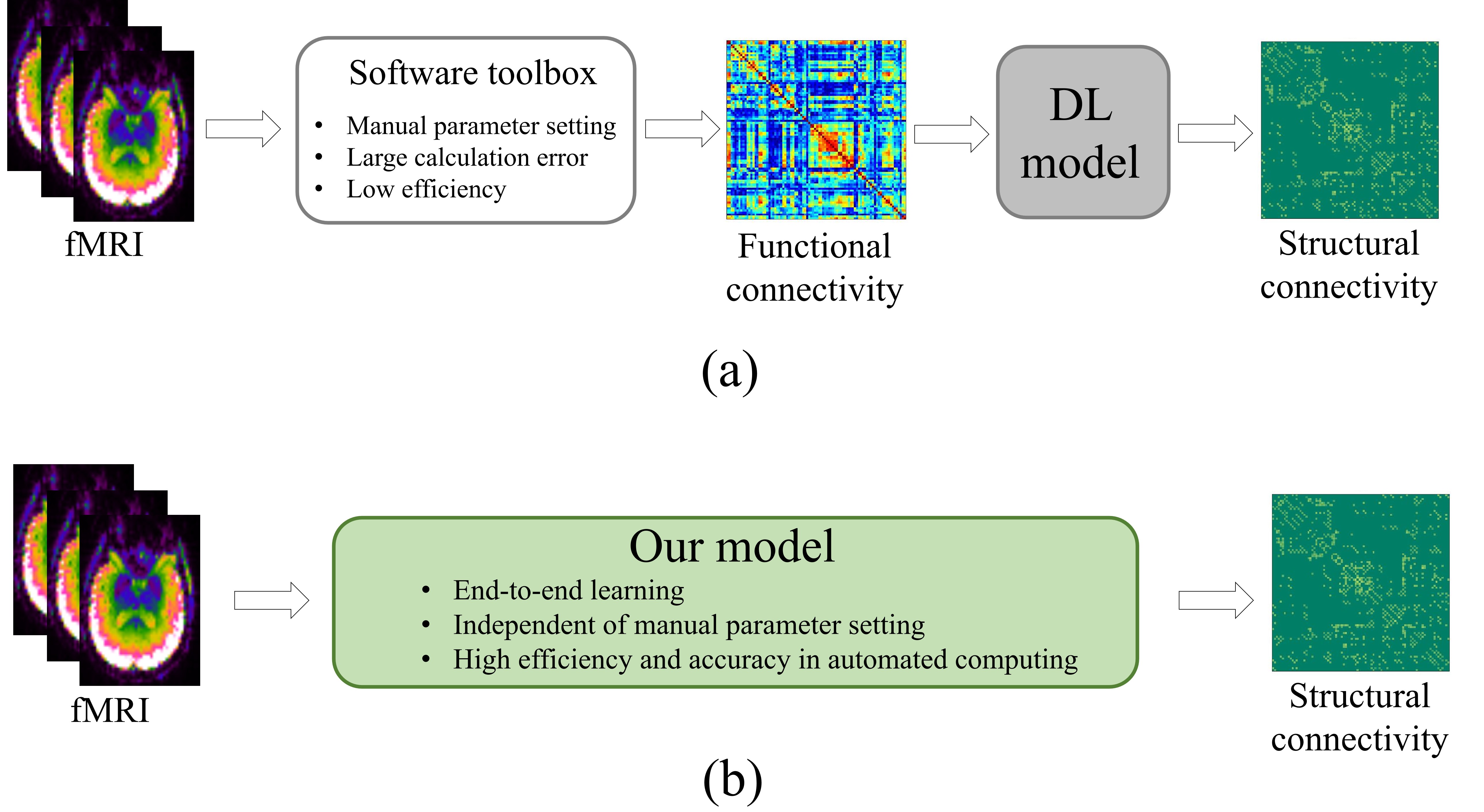
Generative Adversarial Networks (GANs)[27] offer a compelling advantage in medical image computing due to their ability to effectively learn distribution-consistent features [28, 29, 30]. The cross-modal prediction computing allows researchers and healthcare professionals to leverage existing datasets from various modalities, enhancing data utilization and reducing the need for laborious and expensive data collection for each modality separately[31, 32, 33]. To predict SC from brain fMRI in one stage, the GAN-based model remains suitable and effective. The optimized generator maps the fMRI into structural connectivity in an end-to-end manner when the discriminator fails to distinguish the connectivity distribution. However, the challenge of instability and mode collapse during adversarial training still needs to be fully addressed. Meanwhile, denoising diffusion probabilistic models (DDPM)[34, 35] have gained considerable attention in machine learning and demonstrated promising performance in image generation[36, 37]. DDPM utilizes a diffusion process to model the data distribution, gradually transforming Gaussian noise into a clean sample through a lot of successive steps. The main advantage is the high quality and diversity of generation performance, which can address the problems of mode collapse and training instability in GAN-based models. But thousands of denoising steps result in low efficiency in generating samples. Therefore, combing GAN and DDPM is an alternative way to efficiently generate samples with high quality and diversity.

Based on the aforementioned insights, we propose DiffGAN-F2S, a symmetric and efficient denoising diffusision generative adversarial network transmitting fMRI to SC in an end-to-end manner. The fMRI is integrated as a condition in the denoising process of DDPM for structural connectivity prediction, where each denoising step is accompanied by a generator and a discriminator. Firstly, the prior anatomical knowledge is used to transform each 3D volume into multiple ROIs (Regions of Interest) and calculate the preliminary ROI-based time series. Secondly, the empirical SC is transformed into a Gaussian matrix with thousands of difusion steps. Thirdly, the preliminary ROI-based time series and the noisy Gaussian matrix are sent into the symmetric graph generator for noise removal; the dual-channel multi-head spatial attention (DMSA) and GCN-based modules in the generator model global-local interactions between brain regions to capture topological connectivity patterns; meanwhile, the connectivity discriminator is used to constrain the distribution of denoised SC to follow the distribution of empirical SC. After a few denoising steps, the proposed DiffGAN-F2S finally enables the precise and effective mapping of fMRI to structural connectivity. To summarize, the primary contributions are as follows:

• The proposed model is the first work to translate brain fMRI into structural connectivity in the field of cross-modal image-to-graph prediction. By leveraging the unique strengths of diffusion models and generative adversarial networks, it achieves high-fidelity and diverse structural connectivity prediction with efficient generation through a few denoising steps.

• The symmetric graph generator is designed to denoise the fMRI guided by the symmetrical connectivity. Through the dual-channel multi-head spatial attention (DMSA) and GCN-based modules, the generator first captures global relations among direct and indirect connected brain regions, then models the local brain region interactions, which uncovers the complex mapping between fMRI and structural connectivity.

• The spatially connected consistency loss is devised to preserve both global and local topological characteristics, guiding the denoising process to accurately predict intrinsic structural patterns.

The structure of this work is outlined as follows: Section  2 presents the main architecture of the proposed DiffGAN-F2S model. In Section  3, we apply the proposed model to public datasets and conduct result analysis. Section  4 demonstrates the reliability of our findings and summarizes the key observations in this study.

Figure 2: The structure of the proposed DiffGAN-F2S. (a) The empirical SC $A_{0}$ is diffused to the Gaussian matrix $A_{T}$ with T steps. (b) The fMRI is the condition and guides the denoising process from the Gaussian matrix $A_{T}$ to the predicted SC $A_{0}^{\prime}$. (c) the details of the generative adversarial network from the $t+d$-th and $t$-th denoising steps.

2 Method

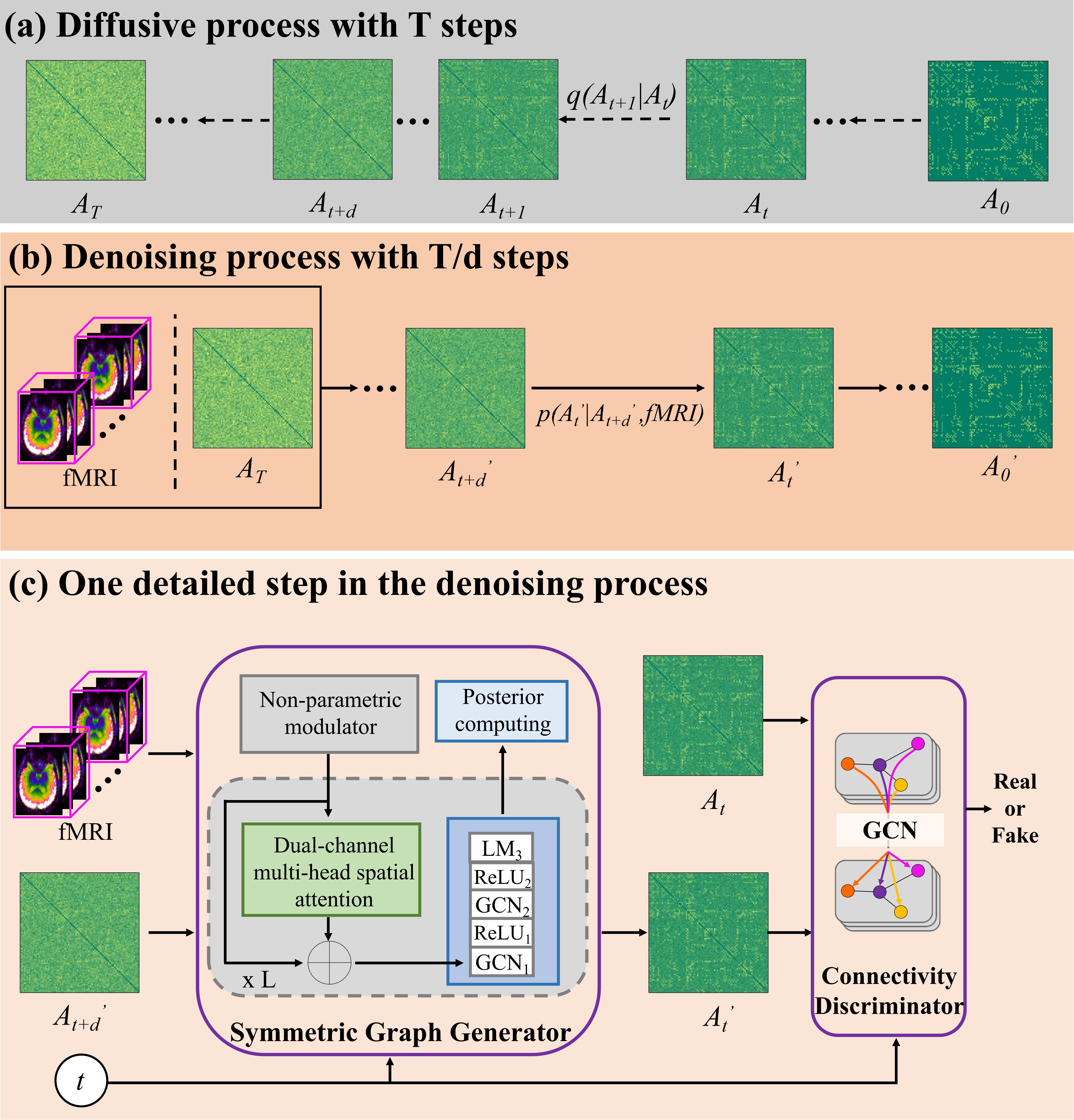
The architecture of the proposed model is shown in Fig. 2. It consists of two parts: the diffusive process and the denoising process. The DiffGAN-F2S first models the truth distribution of noisy SC at different steps by persistently injecting Gaussian noise into empirical SC ($\boldsymbol{A}_{0}$). After T steps, the empirical $\boldsymbol{A}_{0}$ can be transmitted into the Gaussian matrix $\boldsymbol{A}_{T}$. Secondly, the brain fMRI is involved in the denoising process as a condition to help predict clean SC $\boldsymbol{A}_{0}^{\prime}$. It should be stressed that each denoising step is composed of a generator and a discriminator (Fig. 2(c)). During the model training, three kinds of loss functions are devised to optimize the generator for precise cross-modal connectivity prediction, including the denoising adversarial loss, the spatially connected consistency loss, and the mean absolute error (MAE) loss.

2.1 Symmetric diffusive process

The diffusive process of Denoising Diffusion Probabilistic Models (DDPM) involves a fascinating approach to generating a Gaussian matrix by gradually transforming empirical SC into Gaussian noise through a sufficient number of T steps. At each step, a weight is applied to the Gaussian noise to establish a Markov chain. These weights are predefined as a variance schedule: $\beta_{1},\beta_{2},...,\beta_{T}$. To simplify the process, the intermediate noisy SC $\boldsymbol{A}_{t+1}$ is computed from the previous noisy matrix $\boldsymbol{A}_{t}$ at step $t$ using the following formulas:

$$\boldsymbol{A}_{t+1}=\sqrt{1-\beta_{t}}\boldsymbol{A}_{t}+\frac{\sqrt{\beta_{t}}}{2}(\boldsymbol{\epsilon}+\boldsymbol{\epsilon}^{s}),\quad\boldsymbol{\epsilon}\sim\mathcal{N}(\mathbf{0},\boldsymbol{I})$$ (1)

where $\boldsymbol{\epsilon}^{s}$ represents the transpose of $\boldsymbol{\epsilon}$, and $\mathcal{N}$ is the Gaussian distribution. The diagonal element of $\boldsymbol{\epsilon}$ is set to 0. The second term to the right of the equal sign is used to generate values in the range of $0\sim 1$.$\beta_{t}\in(0,1)$ is defined the same as previous works[34]. The noisy matrix $\boldsymbol{A}_{T}$ at the last diffusion step is given:

$$\boldsymbol{A}_{T}=\sqrt{\tilde{\eta}_{t}}\boldsymbol{A}_{0}+\frac{\sqrt{1-\tilde{\eta}_{t}}}{2}(\boldsymbol{\epsilon}_{t}+\boldsymbol{\epsilon}_{t}^{s})$$ (2)

here, $\eta_{t}=1-\beta_{t},\tilde{\eta}_{t}=\prod_{j=1}^{t}\eta_{j}$, $\boldsymbol{\epsilon}_{t}$ means the sampled noise matrix from $\mathcal{N}(\mathbf{0},\boldsymbol{I})$ at t step. are sampled from the Gaussian distribution with the same size of $\boldsymbol{A}_{t}$. Setting a large value for $T$ guarantees that the noisy sample $\boldsymbol{A}_{t}$ closely approximates a Gaussian distribution.

Figure 3: The structure of the dual-channel multi-head spatial attention module. The input is the noisy connectivity and ROI features, and the output is the updated ROI features.

2.2 Symmetric denoising process

The aim of our work is to predict individual SC from brain fMRI; the traditional denoising process of DDPM cannot achieve this goal. Therefore, we use the fMRI as a condition to guide the denoising process. Besides, large $T$ needs much more computing time and lowers the SC prediction efficacy. We reduce the denoising steps into $T/d$ steps, where each step is modeled with a conditional generative adversarial network. Here, $d$ represents the skipping steps. Specifically, the symmetric graph generator $\boldsymbol{G}_{\theta}(\boldsymbol{A}_{t+d}^{\prime},\boldsymbol{fMRI},t)$ accepts the noisy sample $\boldsymbol{A}_{t+d}^{\prime}$, the conditional $\boldsymbol{fMRI}$, the $t$-th learnable embedding $\boldsymbol{e}_{t}^{g}$, and predicts $A_{t}^{\prime}\sim p(A_{t}^{\prime}|A_{t+d}^{\prime},fMRI)$. These embeddings are added as biases onto latent feature maps and control the generation difference during denoising steps. Meanwhile, the connectivity discriminator $\boldsymbol{D}_{\phi}(\boldsymbol{A}_{t}or\boldsymbol{A}_{t}^{\prime},t)$ measures the connectivity distribution difference between real (empirical) $q(\boldsymbol{A}_{t}|\boldsymbol{A}_{0},t)$ and fake (predicted) $p(\boldsymbol{A}_{t}^{\prime}|\boldsymbol{A}_{t+d}^{\prime},\boldsymbol{fMRI}))$. The temporal embedding $\boldsymbol{e}_{t}^{d}$ also involved the discriminating computation as a bias term. The detailed structure of the generator and discriminator is shown in Fig. 2(c).

2.2.1 Symmetric graph generator

The non-parametric modulator (NPM) is used to transform the raw brain fMRI into preliminary ROI-based time series. As the anatomical atlas (i.e., Anatomical Automatic Labeling, AAL90) divides the whole brain into 90 regions of interest and defines the location and volume for each ROI, we resample each 3D volume of fMRI into the same size of the AAL90 atlas and apply a pixel-level dot product between them. The mean pixel value among the same ROI comprises one point of the ROI-based time series. The whole procedure has no learnable parameters. The output of this modulator is defined as the primary ROI-based time series $\boldsymbol{F}_{T}=NPM(\boldsymbol{fMRI})$.

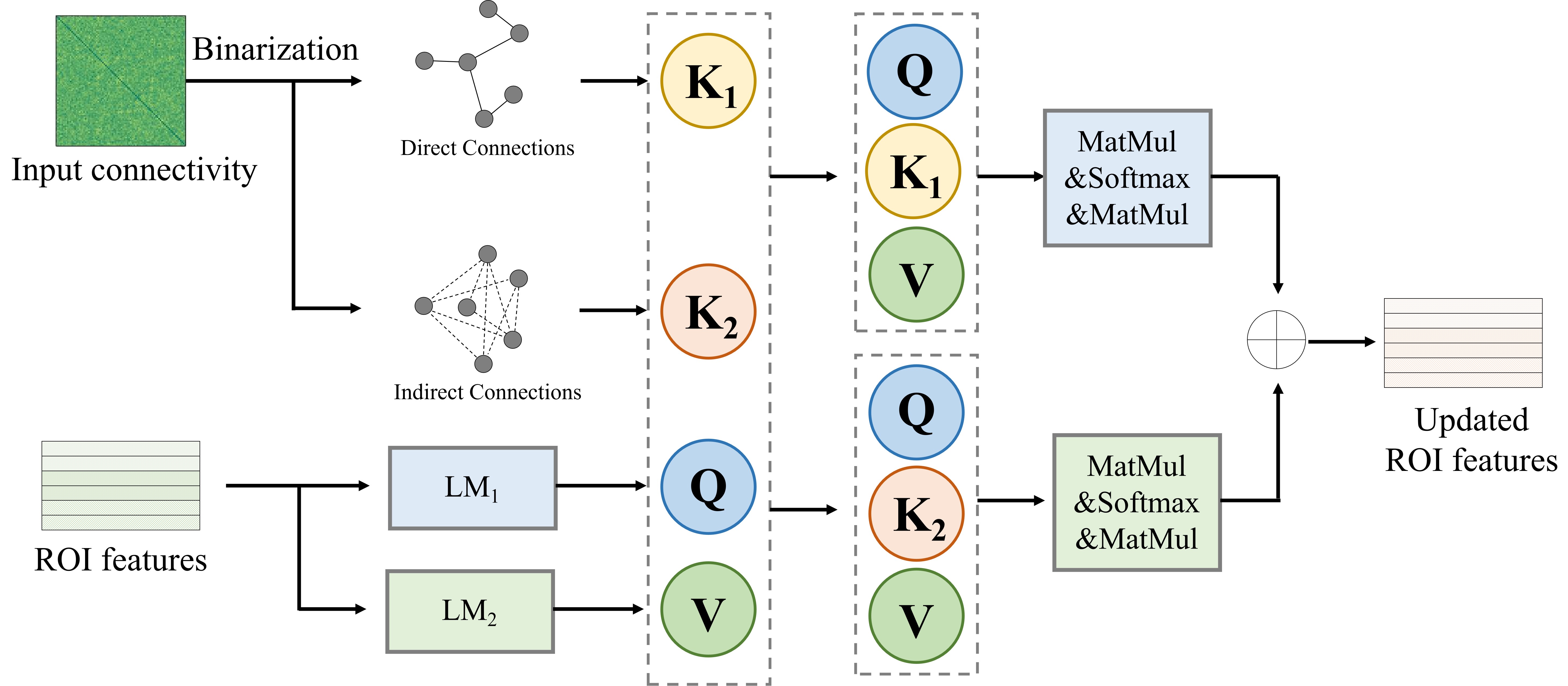
The the $\boldsymbol{F}_{t+d}$ and $\boldsymbol{A}_{t+d}^{\prime}$ pass through $L$ layers consisting of one dual-channel multi-head spatial attention (DMSA) module and one GCN-based module to predict blurred SC ($\boldsymbol{\dot{A}}_{0}$) at the $t+d$ step. As shown in Fig. 3, the DMSA captures global relations among directly and indirectly connected brain regions. For the convenience of description, we specify one layer, denote the input connectivity as $\boldsymbol{A}_{t+d}^{\prime}$, and denote ROI features as $\boldsymbol{F}_{t+d}$. We compute the Query ($\boldsymbol{Q}$), Key ($\boldsymbol{K}_{1}$,$\boldsymbol{K}_{2}$), and Value ($\boldsymbol{V}$) for the ROI features. The $\boldsymbol{K}_{1}$ and $\boldsymbol{K}_{2}$ stands for direct and indirect connected ROI features. When computing the attention values, the directly connected ROI Keys are combined with Queries to obtain attention maps. We denote the $\cup$ and $\bar{\cup}$ as direct and indirect connected brain region containers. The computation of these modes is expressed by:

$$\boldsymbol{F}^{dmsa} =Att_{1}(\boldsymbol{Q},\boldsymbol{K_{1}})\boldsymbol{V}+Att_{2}(\boldsymbol{Q},\boldsymbol{K_{2}})\boldsymbol{V}+\boldsymbol{F}_{t+d}$$ (3)

$$=\operatorname{softmax}\left(\frac{\boldsymbol{Q}\boldsymbol{K}_{1}^{s}}{\sqrt{Num(\cup)}}\right)\boldsymbol{V}+\operatorname{softmax}\left(\frac{\boldsymbol{Q}\boldsymbol{K}_{2}^{s}}{\sqrt{Num(\bar{\cup})}}\right)\boldsymbol{V}+\boldsymbol{F}_{t+d}$$

$$\boldsymbol{F}^{graph}=LM_{3}(ReLU_{2}(GCN_{2}(ReLU_{1}(GCN_{1}(\boldsymbol{F}^{dmsa})+\boldsymbol{e}_{t}^{g}))+\boldsymbol{e}_{t}^{g})+\boldsymbol{e}_{t}^{g})$$ (4)

To be specific, for the $i$-th brain region, the directly connected brain container is denoted as $\cup_{i}$. The attention value between $i$-th and $j$-th brain regions can be computed by:

$$Att_{1,ij}=\frac{\boldsymbol{V}_{ij}\boldsymbol{K}_{1,ij}/\sqrt{Num(\cup)}}{\sum_{k\in\cup_{i}}\left(\boldsymbol{V}_{ij}\boldsymbol{K}_{1,ij}/\sqrt{Num(\cup)}\right)}$$ (5)

This formula can also be applied to the calculation of attention value in brain regions that are indirectly connected.

The posterior computing module (PCD) first translates the ROI-based features $\boldsymbol{F}^{graph}$ into symmetrically blurred $\boldsymbol{\dot{A}}_{0}$, then predicts noisy SC at the $t$-th step by posterior sampling strategy. The computing formula is given:

$$\boldsymbol{\dot{A}}_{0}=\sigma(\boldsymbol{F}^{graph}(\boldsymbol{F}^{graph})^{s})-\boldsymbol{E}$$ (6)

$$\boldsymbol{A}_{t}^{\prime}=\sqrt{\tilde{\eta}_{t}}\boldsymbol{\dot{A}}_{0}+\frac{\sqrt{1-\tilde{\eta}_{t}}}{2}(\boldsymbol{\epsilon}_{t}+\boldsymbol{\epsilon}_{t}^{s})$$ (7)

The output $\boldsymbol{A}_{t}^{\prime}$ is then used to predict $\boldsymbol{A}_{t-d}^{\prime}$. $\boldsymbol{E}$ is an identity matrix. After $T/d$ steps, we can obtain the final clean SC $\boldsymbol{A}_{0}^{\prime}$.

2.2.2 Connectivity discriminator

The discriminator aims to distinguish whether the noisy SC comes from the generator or the empirical method. The network structure is designed with three GCN layers, where the edge is the noisy SC ($\boldsymbol{A}_{t}$, or $\boldsymbol{A}_{t}^{\prime}$) , and the node feature is defined with a one-hot vector. For each GCN layer, the temporal embedding ($\boldsymbol{e}_{t}^{d}$) is inserted as a bias. After three GCN layers, the ROI feature is averaged and mapped into one scalar. The output value of 0 or 1 indicates the fake (predicted) or real (empirical) SC.

2.3 Loss function

To enhance the quality of the predicted SC, a hybrid objective function is devised for model optimization. Firstly, the generative adversarial loss constrains the predicted SC and the empirical SC in distribution consistency by computing the discriminative difference between them.

$$\begin{array}[]{r}\mathcal{L}_{D}=\frac{d}{T}\sum_{t\geq 1}\mathbb{E}_{q\left(\mathbf{A}_{t}\mid\mathbf{A}_{0}\right)}\left[\left(D_{\phi}\left(\mathbf{A}_{t},t\right)-1\right)^{2}\right]\\ +\mathbb{E}_{p_{\theta}\left(\mathbf{A}_{t}^{\prime}\mid\mathbf{A}_{t+d}^{\prime}\right)}\left[D_{\phi}\left(\mathbf{A}_{t}^{\prime},t\right)^{2}\right]\end{array}$$ (8)

$$\begin{array}[]{r}\mathcal{L}_{G}=\frac{d}{T}\sum_{t\geq 1}\mathbb{E}_{p_{\theta}\left(\mathbf{A}_{t}^{\prime}\mid\mathbf{A}_{t+d}^{\prime}\right)}\left[(D_{\phi}\left(\mathbf{A}_{t}^{\prime},t\right)-1)^{2}\right]\end{array}$$ (9)

Besides, to enforce an additional element-wise constraint on the generator, the MSE loss is added to the adversarial loss by measuring the edge strength difference between the predicted SC and the empirical SC. This loss can make the generator stable when predicting SC. The MSE loss is defined as follows:

$$\mathcal{L}_{MSE}=\frac{d}{T}\sum_{t\geq 1}||\boldsymbol{\dot{A}}_{0,t}-\mathbf{A}_{0}||$$ (10)

Furthermore, to capture the local and global graphical properties, the spatially connected consistency loss is devised to guide the denoising process to accurately predict intrinsic structural patterns.

$$\mathcal{L}_{SCC}= \frac{\sum(\boldsymbol{A}_{0}^{\prime}-\bar{\boldsymbol{A}_{0}^{\prime}})\cdot(\boldsymbol{A}_{0}-\bar{\boldsymbol{A}_{0}})}{\sqrt{\sum(\boldsymbol{A}_{0}^{\prime}-\bar{\boldsymbol{A}_{0}^{\prime}})^{2}}\cdot\sqrt{\sum(\boldsymbol{A}_{0}-\bar{\boldsymbol{A}_{0}})^{2}}}$$ (11)

$$+\sum_{k}||\sum_{i\neq k\neq j,\boldsymbol{A}_{0}^{\prime}}\frac{\kappa_{ij}(k)}{\kappa_{ij}}-\sum_{i\neq k\neq j,\boldsymbol{A}_{0}}\frac{\kappa_{ij}(k)}{\kappa_{ij}}||$$

Here, the first term measures the overall similaity between predicted and empirical SC, and the second term computes the betweenness centrality (BC) to measure the local topological similarity. $\kappa_{ij}(k)$ is the number of shortest paths through $k$-th ROI from ROI $i$ to ROI $j$, $\kappa_{ij}$ represents all the number of shortest paths between ROI $i$ and ROI $j$.

The optimization strategy of the proposed DiffGAN-F2S is illustrated using pseudo-code. The Algorithm 1 and Algorithm 2 display the training process and sampling process, respectively.

Algorithm 1 Training of DiffGAN-F2S

1:$\boldsymbol{A}_{0}$: empirical SC
     $\boldsymbol{fMRI}$: conditional imaging
     $\boldsymbol{G}_{\theta}$: symmetric graph generator with parameter $\theta$
     $\boldsymbol{D}_{\phi}$: connectivity discriminator with parameter $\phi$
     $T$: diffusion step number
     $\beta_{i},i=1,2,...,T$: predefined variance schedle
     $d$: skipping step number

2:$\boldsymbol{G}_{\theta}$ and $\boldsymbol{e}^{g}$

3:initialize the $\theta$ and $\phi$, the temporal embedding $\boldsymbol{e}^{g}$ and $\boldsymbol{e}^{d}$;

4:repeat

5:     $t\sim Uniform({d,2d,...,T})$

6:     Sample $\boldsymbol{\epsilon}_{t}\sim\mathcal{N}(\mathbf{0},\boldsymbol{I})$

7:     Compute the $\boldsymbol{A}_{t}$ and $\boldsymbol{A}_{t+d}$ using Eq.( 1)

8:     Propogate the tuple ($\boldsymbol{A}_{t+d},\boldsymbol{fMRI},\boldsymbol{e}_{t}^{g}$) to $\boldsymbol{G}_{\theta}$ to obtain
     predicted SC $\boldsymbol{\dot{A}}_{0,t}$ and noisy SC $\boldsymbol{A}_{t}^{\prime}$

9:     Propogate the tuple ($\boldsymbol{A}_{t},\boldsymbol{e}^{d}$) or ($\boldsymbol{A}_{t}^{\prime},\boldsymbol{e}^{d}$) to $\boldsymbol{D}_{\phi}$ to predict
     true or false

10:     Compute the $\mathcal{L}_{D}$ using Eq.( 8) and update $\phi$ by back
     propagating the gradient $-\nabla_{\phi}\mathcal{L}_{D}$

11:     Compute the combination of Eq.( 9),Eq.( 10),Eq.( 11),
     and update $\phi$ by back-propagating the gradient
     $-\nabla_{\theta}(\mathcal{L}_{G}+\mathcal{L}_{MSE}+\mathcal{L}_{SCC})$

12:until converged

Algorithm 2 Inference procedure of DiffGAN-F2S

1:$\boldsymbol{fMRI}$: conditional imaging
     $\boldsymbol{G}_{\theta}$: symmetric graph generator with parameter $\theta$
     $T$: number of diffusion steps
     $\boldsymbol{e}^{g}$: temporal embedding of the generator

2:Clean SC $\boldsymbol{A}_{0}^{\prime}$

3:Sample Gaussian SC $\boldsymbol{A}_{T}=(\boldsymbol{\epsilon}+\boldsymbol{\epsilon}^{s})/2$, $\boldsymbol{\epsilon}\sim\mathcal{N}(\mathbf{0},\boldsymbol{I})$

4:for $t=T-d$ to $0$ do

5:     Forward-propagate the tuple ($\boldsymbol{A}_{t+d},\boldsymbol{fMRI},\boldsymbol{e}_{t}^{g}$) to $\boldsymbol{G}_{\theta}$ to
     compute noisy SC $\boldsymbol{A}_{t}^{\prime}$

6:     $t=t-d$

7:end for

8:Return $\boldsymbol{A}_{0}^{\prime}$

Figure 4: Predicted structural connectivities at different diffusive steps by the proposed model.

3 Experiments

3.1 Datasets

To test our model’s performance, we selected two categories of 240 patients (i.e., normal control and mild cognitive impairment) from the publicly available Alzheimer’s Disease Neuroimaging Initiative (ADNI) dataset. Each category has 120 subjects. Mild cognitive impairment (MCI) includes early MCI and late MCI. Every subject was scanned with fMRI and DTI by a 3T magnetic resonance instrument. The DTI is preprocessed by the PANDA[38] toolbox. Based on the anatomical automatic labeling (AAL90) atlas [39], the detailed preprocessing procedures are described in the work [40]. The output of preprocessing DTI is the empirical SC ($\boldsymbol{A}_{0}$) with the size of $90\times 90$. For the fMRI preprocessing, we abandon the preprocessing procedures [41] and utilize an anatomical atlas file $aal.nii$ to transmit the brain fMRI into ROI-based time series without any parameters. The output of fMRI preprocessing is a primary sample $\boldsymbol{F}$ with a size of $90\times 187$.

3.2 Training Settings and Evaluation Metrics

The aim of our model is to transform the fMRI into structural connectivity step by step. During the model training, we utilize the following parameters: $L=3$, $T=100$. The skipping step number $d$ is set as 10. The code is written using the Pycharm tool and runs on the Windows 11 system. The total training epochs are 1000, with a learning rate of $10^{-3}$. The Adam algorithm with default settings is selected to update the weights of the generators and discriminators. The batch size is set to 64.

Figure 5: Comparison of the predicted SCs and empirical SCs selected from two subjects.

Figure 6: Comparison of group SCs between empirical and predicted SCs. The right column demonstrates the highly correlation between the empirical and predicted SCs.

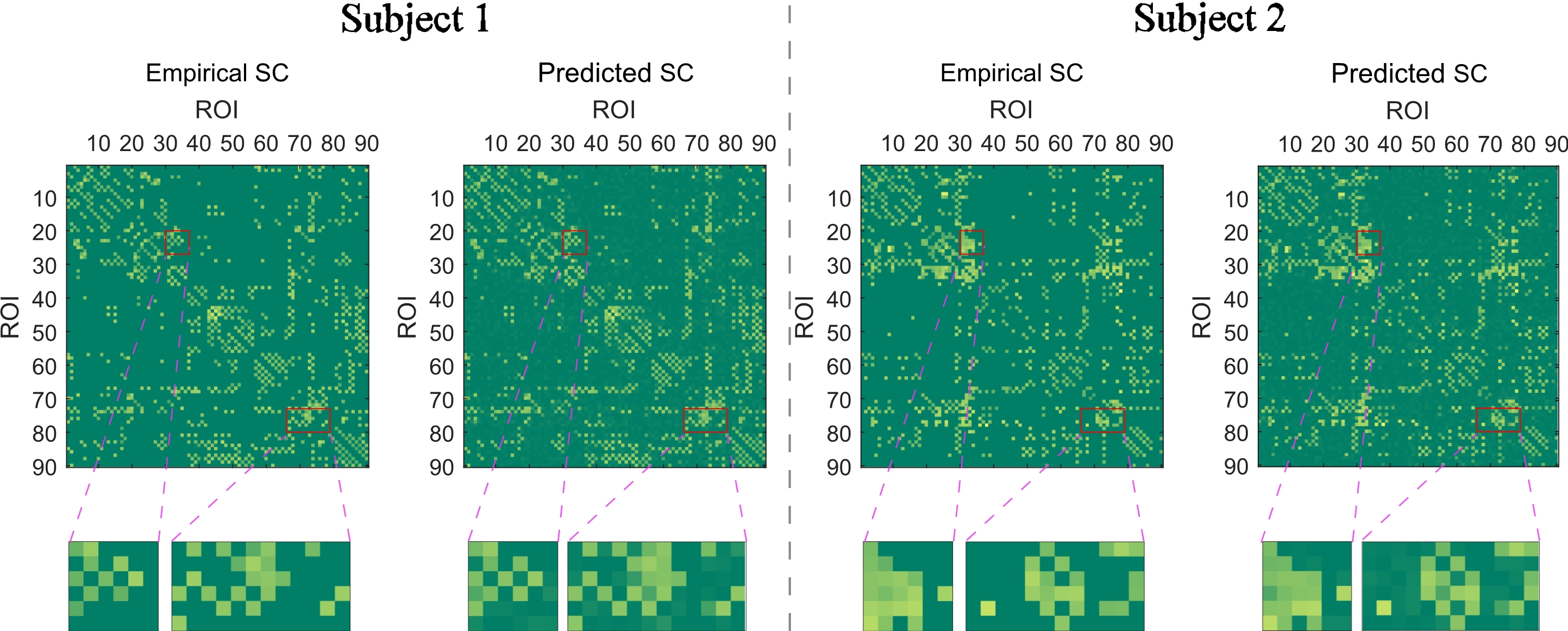
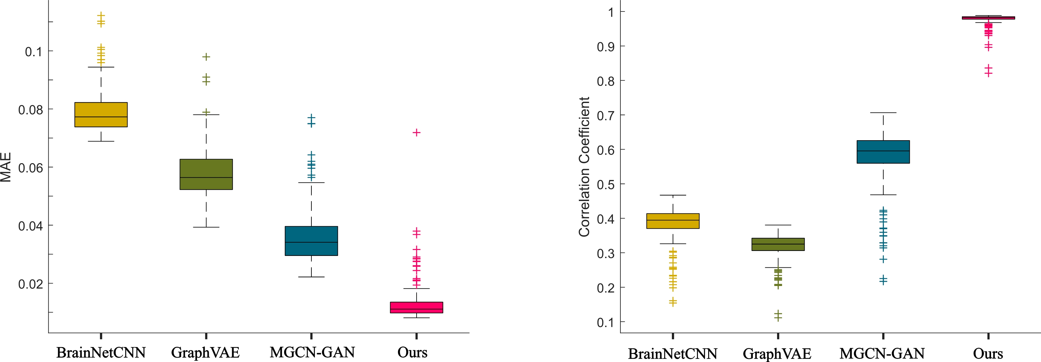
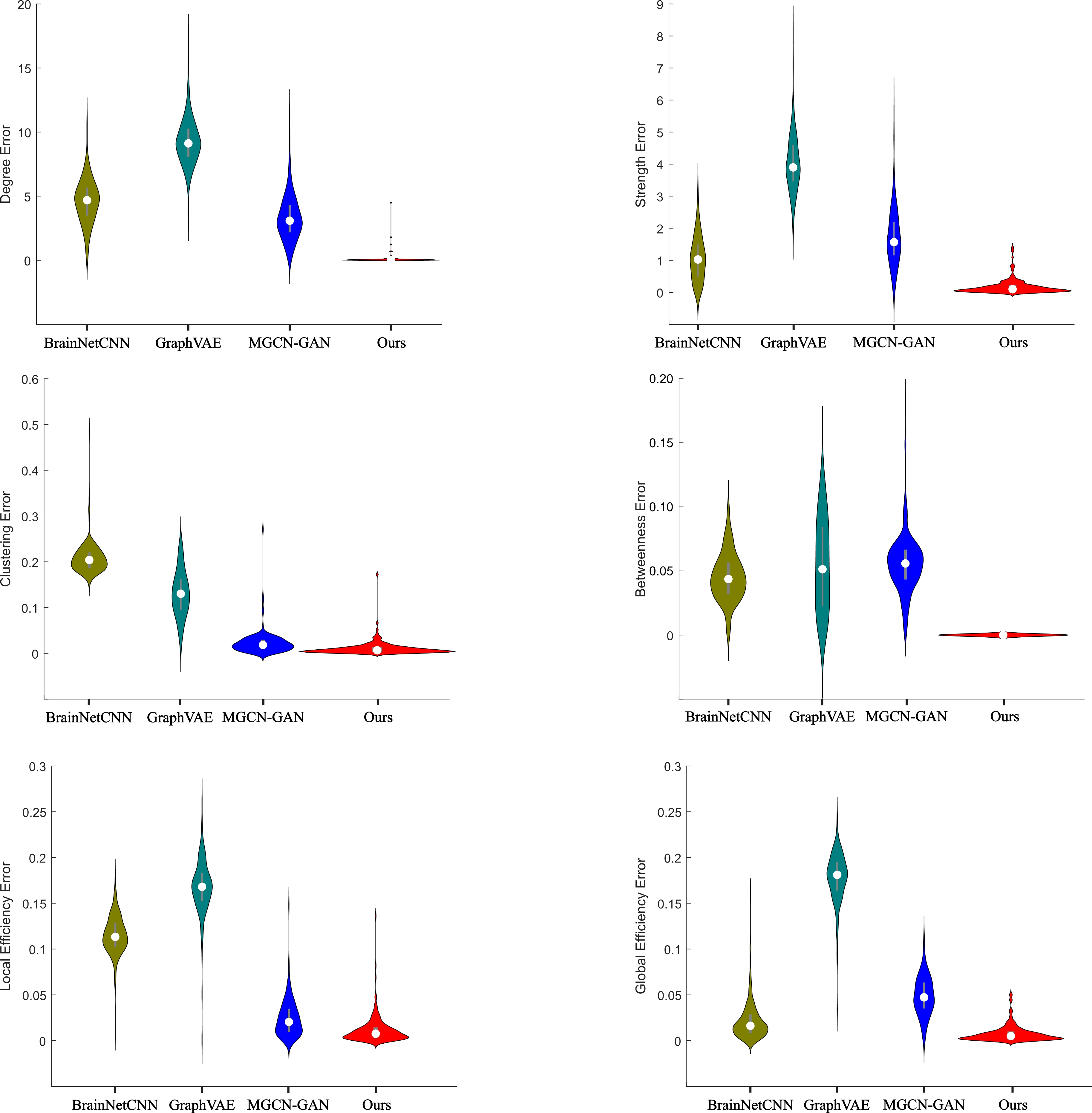
The qualitative results are presented through global and local detail maps. Besides, the predicted results are quantitatively evaluated by eight metrics, including the mean absolute error (MAE), the correlation coefficient (CC), the degree error, the strength error, the clustering error, the betweenness error, the local efficiency error, and the global efficiency error. The former two metrics are the traditional image evaluation methods, and the latter six metrics are the commonly used graph-based measurements. Further, we conduct ROI-based and connectivity-based comparisons to examine our model’s generation performance.

Figure 7: The MAE and correlaltion coefficient between predicted and emprical SCs using different models.

Figure 8: Comparison of six graph metrics using four different models. The top row is the mean degree error and conenctivity strength error; the middle row is the mean clustering error and betweenness error; the third row is the local and global efficiency error.

3.3 Denoised and Prediction Results

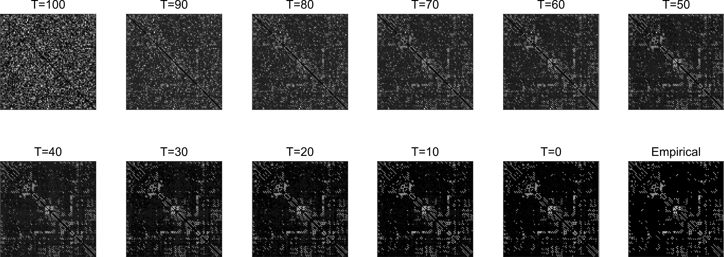
In our experiments, given brain fMRI, our model can denoise a symmetrical Gaussian into corresponding strucral connectivity. Fig. 4 shows the detailed denoised SCs at 10 representative steps. As the time step decreases to 0, the noise is gradually removed and the empirical connectivity features are preserved. When t = 0, the predicted SC closely resembles the empirical SC. To qualitatively demonstrate the generation performance, two representative subjects are displayed in Fig. 5. For each subject, both the global and local connectivity patterns are highly preserved. Furthermore, we investigate the group-level connectivity patterns between the empirical and predicted SCs. Specifically, we mean all the predicted SCs and all the empirical SCs, respectively. The subsequent predicted group SC and emprical group SC are reshaped into one-dimensional vectors, which are displayed in a plane. As shown in Fig. 6, the connectivity element value ranges from 0.0 to 0.8. Each blue circle represents each element in predicted SC and emirical SC. Almost all the blue circles are distributed diagonally. It means there is a high correlation between the empirical and predicted SCs. Also, there are few outliers that deviate from the diagonal line. This means that there are some connections in predicted SCs that are not present in empirical SCs. The possible reason is that the predicted SCs contain little functional-specific information.

Figure 9: Comparison of the top 10 percent and top 20 percent ROIs between the empirical method and our model; the right column is the ROI distribution difference between them.

To quantitatively evaluate the quality of predicted SCs, we add three other models for comparison. Considering no studies have focused on the tasks of transforming images into graphs, we use functional connectivity (fC) as input in these three models. (1) The BrainNetCNN model  [42] with the edge-to-edge convolutional filters. (2) the graph variational autoencoder (GraphVAE)  [43], the node features are set as one-hot vectors. (3) the multi-GCN-based GAN model  [25]. As shown in Fig. 7, the boxplots show our model achieves the best performance with the mean MAE value of 0.013 and the mean correlation coefficient of 0.976. The Fig. 8 shows the distribution and density of graph metric errors between predicted SCs and empirical SCs. Among the six metrics, our model demonstrates the most concentrated distribution around the median value. This indicates that our model performs the best in the task of generating SC from fMRI among these four models.

Figure 10: Comparison of the top ten increased and reduced connections between the empirical method and our model; the different connections are displayed in the right column.

3.4 Analysis of Effective Connectivity

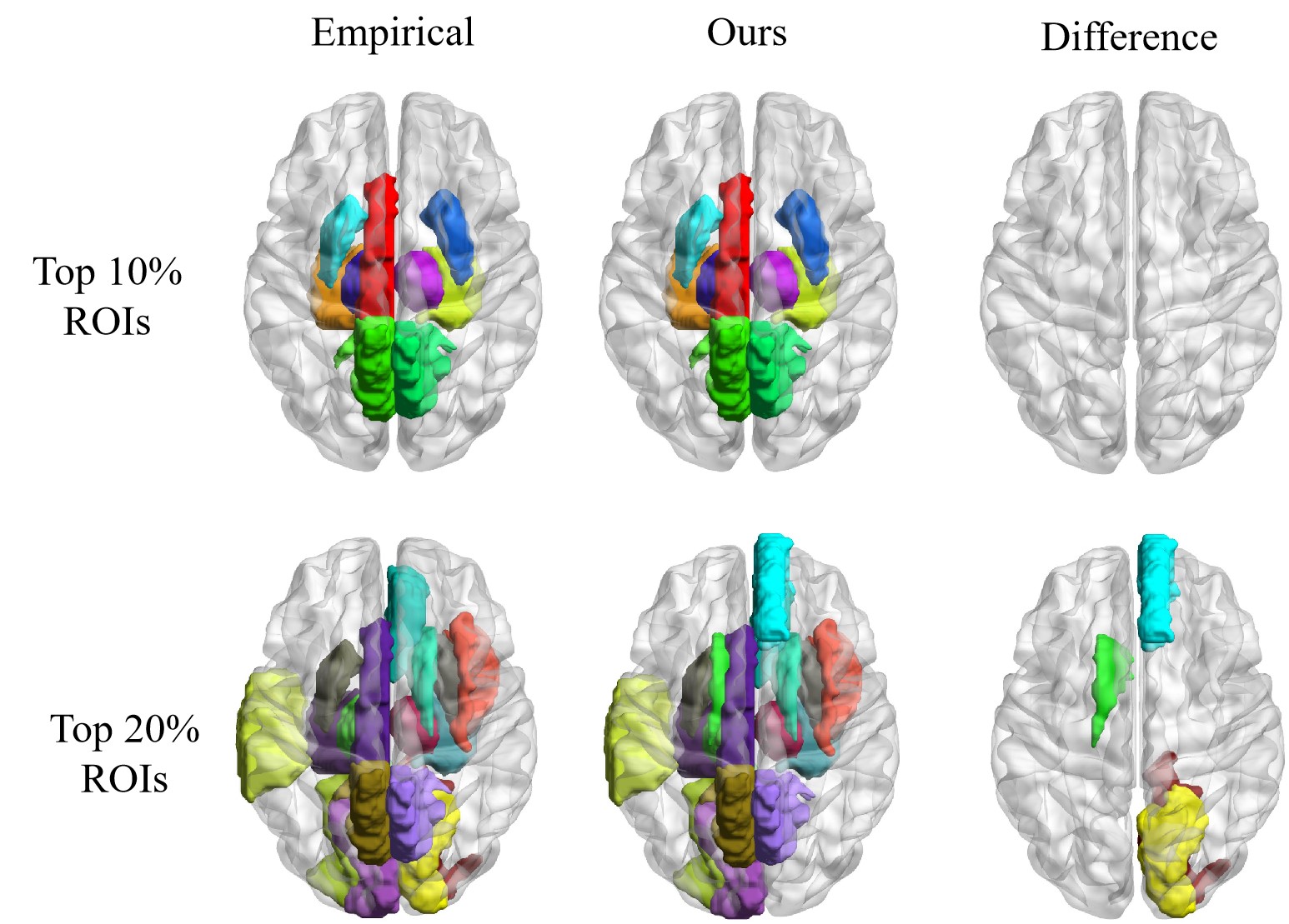
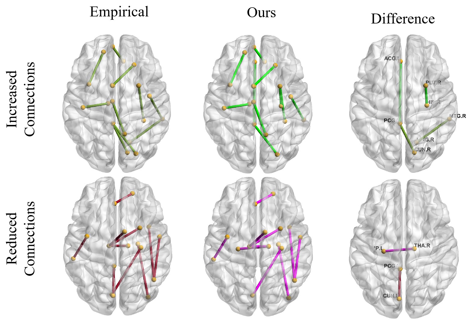
The connectivity features are important for analyzing brain disease. In our experiment, we investigate the connectivity-based analysis between predicted SCs and empirical SCs. Usually, we first compute the average SC for each group (i.e., NC and MCI) and then subtract the average SC of NC from the average SC of MCI. The different elements are the abnormal connections. Analyzing these abnormal findings can help improve disease diagnosis accuracy and detect potential biomarkers. To compare the important ROIs, we sum the connection strength change for each ROI and sort them in descending order. The top 10 percent and top 20 percent ROIs are displayed in Fig. 9. The top 10 percent of ROIs are the same for both empirical and predicted SCs. Out of the top 20 percent ROIs, there are two that are not consistent. The CAL.R and LING.R calculated from empirical SCs are not presented in the predicted SCs. These two ROIs are presented at the top 30% ROIs calculated from the predicted SCs. To compare the top 10 abnormal connections between NC and MCI, we select the top 10 positive values and the last 10 negative values in the subtracted SC. These connections are displayed in Fig. 10. Both the empirical method and ours show most of the common connections except one or two connections, which means we can utilize our model to generate SCs and obtain the same analysis results.

Table 1: Comparison of SC prediction performance by the proposed model using different loss functions.

	MAE	CC	Degree Error	Strength Error	Clustering Error	Betweenness Error	Local efficiency Error	Global efficiency Error
DiffGAN-F2S w/o $L_{GAN}$	0.035 ($\pm$0.012)	0.893 ($\pm$0.049)	3.541 ($\pm$4.212)	0.363 ($\pm$0.955)	0.108 ($\pm$0.035)	0.275 ($\pm$0.179)	0.090 ($\pm$0.020)	0.027 ($\pm$0.014)
DiffGAN-F2S w/o $L_{SCC}$	0.028 ($\pm$0.011)	0.931 ($\pm$0.038)	1.985 ($\pm$4.187)	0.351 ($\pm$0.837)	0.068 ($\pm$0.033)	0.286 ($\pm$0.210)	0.058 ($\pm$0.020)	0.021 ($\pm$0.013)
DiffGAN-F2S	0.013 ($\pm$0.007)	0.976 ($\pm$0.021)	0.416 ($\pm$1.623)	0.164 ($\pm$0.311)	0.016 ($\pm$0.023)	0.010 ($\pm$0.261)	0.015 ($\pm$0.018)	0.008 ($\pm$0.009)

3.5 Ablation Study

The proposed DiffGAN-F2S model aims to denoise the fMRI into structural connectivity. To analyze the influence of the loss functions on generation performance, we remove the adversiral loss and spatially connected consistency loss, respectively. The two variants are (1) DiffGAN-F2S w/o $L_{GAN}$ means removing the connectivity discriminator; and (2) DiffGAN-F2S w/o $L_{SCC}$. The eight metrics introduced are calculated to estimate the generation performance. As shown in Table 1 The DiffGAN-F2S without the connectivity discriminator shows the worst reconstruction performance and most inconsistent graph properties. As the discriminator can constrain the predicted SC in a uniformed distribution with empirical SC, the absence of the discriminator loses some empirical conenctivity patterns. Also, the removal of $L_{SCC}$ fails to capture the global topological characteristics, thus producing a greater MAE of 0.015 than that of DiffGAN-F2S.

4 Discussion and Conclusion

The main difference between our model and previous studies is that we transform the original brain fMRI into structural connectivity in one stage. The proposed model can be easily implemented step by step. The non-parameter transforming step can make use of the previously defined AAL90 atlas to partition each volume into 90 parts for all time points. The subsequent 90 parts can be used as ROI features in the denoising process. At each step of the denoising process, the denoised SC is sent into the discriminator to learn connectivity-consistent patterns with the diffusive SC. Combining the GAN and DDPM can benefit two advantages: the ability to generate high-quality and diverse SCs and the fast denoising computation. Table 1 shows the removal of generators can lead to bad performance in fMRI-to-SC prediction. The proposed model generates good SCs that are very similar to empirical SCs. Both subject-specific and group-based qualitative comparisons demonstrate that the predicted SCs by the proposed model can totally capture the empirical connectivity features. Besides, compared with other competing FC-to-SC models, the proposed model can achieve the best results in terms of MAE, correlation coefficient, degree error, strength error, clustering error, betweenness error, local efficiency error, and global efficiency error. Furthermore, as shown in Fig. 9 and Fig. 10, the connectivity-based analysis results can also prove our model’s effectiveness. The predicted SCs by our model can also achieve the same effect as empirical SCs when analyzing brain disease.

This paper proposes a DiffGAN-F2S model to predict SC from brain fMRI in one stage. The DiffGAN-F2S combines diffusion models and generative adversarial networks to generate high-fidelity SCs through a few denoising steps. Stacking the dual-channel multi-head spatial attention and the GCN-based modules in the symmetric graph generator can capture global relations among direct and indirect connected brain regions. To further preserve global-local topological information, a spatially connected consistency loss is devised to constrain the generator to accurately predict empirical SCs. Experimental results on the public ADNI dataset show the superior generation performance of the proposed model compared to other competing models. The proposed model can also be used to identify diease-related connections and important brain regions, which provides an effective way for fMRI-to-SC prediction for multimodal brain network fusion. The main limitation of this work is that we ignore the directional connections in cross-modal prediction. The directional information between brain regions can make the predicted results more interpretable. In the future, we will extend our work to asymmetry denoising for SC prediction.

Conflict of Interest Statement

The authors declare that the research was conducted in the absence of any commercial or financial relationships that could be construed as a potential conflict of interest.

Reference

References

- [1] Y. Zhan, R. C. Paolicelli, F. Sforazzini, L. Weinhard, G. Bolasco, F. Pagani, A. L. Vyssotski, A. Bifone, A. Gozzi, D. Ragozzino, et al., Deficient neuron-microglia signaling results in impaired functional brain connectivity and social behavior, Nature neuroscience 17 (3) (2014) 400–406.
- [2] J. DeLuca, N. D. Chiaravalloti, B. M. Sandroff, Treatment and management of cognitive dysfunction in patients with multiple sclerosis, Nature Reviews Neurology 16 (6) (2020) 319–332.
- [3] D. Kapogiannis, M. P. Mattson, Disrupted energy metabolism and neuronal circuit dysfunction in cognitive impairment and alzheimer’s disease, The Lancet Neurology 10 (2) (2011) 187–198.
- [4] V. Menon, Large-scale brain networks and psychopathology: a unifying triple network model, Trends in cognitive sciences 15 (10) (2011) 483–506.
- [5] W. Zhuang, J. Wang, C. Chu, X. Wei, G. Yi, Y. Dong, L. Cai, Disrupted control architecture of brain network in disorder of consciousness, IEEE Transactions on Neural Systems and Rehabilitation Engineering 30 (2022) 400–409.
- [6] H.-J. Park, K. Friston, Structural and functional brain networks: from connections to cognition, Science 342 (6158) (2013) 1238411.
- [7] S. J. Wiseman, T. Booth, S. J. Ritchie, S. R. Cox, S. Muñoz Maniega, M. d. C. Valdés Hernández, D. A. Dickie, N. A. Royle, J. M. Starr, I. J. Deary, et al., Cognitive abilities, brain white matter hyperintensity volume, and structural network connectivity in older age, Human Brain Mapping 39 (2) (2018) 622–632.
- [8] F. A. Fox, K. Diers, H. Lee, A. Mayr, M. Reuter, M. M. Breteler, N. A. Aziz, Association between accelerometer-derived physical activity measurements and brain structure: A population-based cohort study, Neurology 99 (11) (2022) e1202–e1215.
- [9] M. Díez-Cirarda, A. P. Strafella, J. Kim, J. Peña, N. Ojeda, A. Cabrera-Zubizarreta, N. Ibarretxe-Bilbao, Dynamic functional connectivity in parkinson’s disease patients with mild cognitive impairment and normal cognition, NeuroImage: Clinical 17 (2018) 847–855.
- [10] E. Fiorenzato, A. P. Strafella, J. Kim, R. Schifano, L. Weis, A. Antonini, R. Biundo, Dynamic functional connectivity changes associated with dementia in parkinson’s disease, Brain 142 (9) (2019) 2860–2872.
- [11] G. Chételat, B. Landeau, E. Salmon, I. Yakushev, M. A. Bahri, F. Mézenge, A. Perrotin, C. Bastin, A. Manrique, A. Scheurich, et al., Relationships between brain metabolism decrease in normal aging and changes in structural and functional connectivity, Neuroimage 76 (2013) 167–177.
- [12] B. Lei, S. Yu, X. Zhao, A. F. Frangi, E.-L. Tan, A. Elazab, T. Wang, S. Wang, Diagnosis of early alzheimer’s disease based on dynamic high order networks, Brain imaging and behavior 15 (2021) 276–287.
- [13] S. Wang, H. Wang, A. C. Cheung, Y. Shen, M. Gan, Ensemble of 3d densely connected convolutional network for diagnosis of mild cognitive impairment and alzheimer’s disease, Deep learning applications (2020) 53–73.
- [14] J. Yu, I. Rawtaer, J. Fam, L. Feng, E.-H. Kua, R. Mahendran, The individualized prediction of cognitive test scores in mild cognitive impairment using structural and functional connectivity features, NeuroImage 223 (2020) 117310.
- [15] J. Sui, X. Li, R. P. Bell, S. L. Towe, S. Gadde, N.-k. Chen, C. S. Meade, Structural and functional brain abnormalities in human immunodeficiency virus disease revealed by multimodal magnetic resonance imaging fusion: association with cognitive function, Clinical Infectious Diseases 73 (7) (2021) e2287–e2293.
- [16] C. Gong, C. Jing, X. Chen, C. M. Pun, G. Huang, A. Saha, M. Nieuwoudt, H.-X. Li, Y. Hu, S. Wang, Generative ai for brain image computing and brain network computing: a review, Frontiers in Neuroscience 17 (2023) 1203104.
- [17] B. Lei, N. Cheng, A. F. Frangi, Y. Wei, B. Yu, L. Liang, W. Mai, G. Duan, X. Nong, C. Li, et al., Auto-weighted centralised multi-task learning via integrating functional and structural connectivity for subjective cognitive decline diagnosis, Medical Image Analysis 74 (2021) 102248.
- [18] S. Yu, S. Wang, X. Xiao, J. Cao, G. Yue, D. Liu, T. Wang, Y. Xu, B. Lei, Multi-scale enhanced graph convolutional network for early mild cognitive impairment detection, in: Medical Image Computing and Computer Assisted Intervention–MICCAI 2020: 23rd International Conference, Lima, Peru, October 4–8, 2020, Proceedings, Part VII 23, Springer, 2020, pp. 228–237.
- [19] J. Huang, L. Zhou, L. Wang, D. Zhang, Integrating functional and structural connectivities via diffusion-convolution-bilinear neural network, in: International Conference on Medical Image Computing and Computer-Assisted Intervention, Springer, 2019, pp. 691–699.
- [20] N. S. Dsouza, M. B. Nebel, D. Crocetti, J. Robinson, S. Mostofsky, A. Venkataraman, M-gcn: A multimodal graph convolutional network to integrate functional and structural connectomics data to predict multidimensional phenotypic characterizations, in: Medical Imaging with Deep Learning, PMLR, 2021, pp. 119–130.
- [21] C. J. Honey, O. Sporns, L. Cammoun, X. Gigandet, J.-P. Thiran, R. Meuli, P. Hagmann, Predicting human resting-state functional connectivity from structural connectivity, Proceedings of the National Academy of Sciences 106 (6) (2009) 2035–2040.
- [22] W. Zhang, L. Zhan, P. Thompson, Y. Wang, Deep representation learning for multimodal brain networks, in: Medical Image Computing and Computer Assisted Intervention–MICCAI 2020: 23rd International Conference, Lima, Peru, October 4–8, 2020, Proceedings, Part VII 23, Springer, 2020, pp. 613–624.
- [23] T. Sarwar, Y. Tian, B. T. Yeo, K. Ramamohanarao, A. Zalesky, Structure-function coupling in the human connectome: A machine learning approach, NeuroImage 226 (2021) 117609.
- [24] Y. Wang, X. Chen, B. Liu, W. Liu, R. M. Shiffrin, Understanding the relationship between human brain structure and function by predicting the structural connectivity from functional connectivity, IEEE Access 8 (2020) 209926–209938.
- [25] L. Zhang, L. Wang, D. Zhu, A. D. N. Initiative, et al., Predicting brain structural network using functional connectivity, Medical image analysis 79 (2022) 102463.
- [26] H. Tang, L. Guo, X. Fu, Y. Wang, S. Mackin, O. Ajilore, A. D. Leow, P. M. Thompson, H. Huang, L. Zhan, Signed graph representation learning for functional-to-structural brain network mapping, Medical image analysis 83 (2023) 102674.
- [27] I. Goodfellow, J. Pouget-Abadie, M. Mirza, B. Xu, D. Warde-Farley, S. Ozair, A. Courville, Y. Bengio, Generative adversarial networks, Communications of the ACM 63 (11) (2020) 139–144.
- [28] W. Yu, B. Lei, S. Wang, Y. Liu, Z. Feng, Y. Hu, Y. Shen, M. K. Ng, Morphological feature visualization of alzheimer’s disease via multidirectional perception gan, IEEE Transactions on Neural Networks and Learning Systems (2022).
- [29] S. You, B. Lei, S. Wang, C. K. Chui, A. C. Cheung, Y. Liu, M. Gan, G. Wu, Y. Shen, Fine perceptive gans for brain mr image super-resolution in wavelet domain, IEEE transactions on neural networks and learning systems (2022).
- [30] S. Wang, Z. Chen, S. You, B. Wang, Y. Shen, B. Lei, Brain stroke lesion segmentation using consistent perception generative adversarial network, Neural Computing and Applications 34 (11) (2022) 8657–8669.
- [31] J. Cai, Z. Zhang, L. Cui, Y. Zheng, L. Yang, Towards cross-modal organ translation and segmentation: A cycle-and shape-consistent generative adversarial network, Medical image analysis 52 (2019) 174–184.
- [32] S. Hu, Y. Shen, S. Wang, B. Lei, Brain mr to pet synthesis via bidirectional generative adversarial network, in: Medical Image Computing and Computer Assisted Intervention–MICCAI 2020: 23rd International Conference, Lima, Peru, October 4–8, 2020, Proceedings, Part II 23, Springer, 2020, pp. 698–707.
- [33] S. Hu, B. Lei, S. Wang, Y. Wang, Z. Feng, Y. Shen, Bidirectional mapping generative adversarial networks for brain mr to pet synthesis, IEEE Transactions on Medical Imaging 41 (1) (2021) 145–157.
- [34] J. Ho, A. Jain, P. Abbeel, Denoising diffusion probabilistic models, Advances in neural information processing systems 33 (2020) 6840–6851.
- [35] A. Q. Nichol, P. Dhariwal, Improved denoising diffusion probabilistic models, in: International Conference on Machine Learning, PMLR, 2021, pp. 8162–8171.
- [36] Y. Xie, Q. Li, Measurement-conditioned denoising diffusion probabilistic model for under-sampled medical image reconstruction, in: International Conference on Medical Image Computing and Computer-Assisted Intervention, Springer, 2022, pp. 655–664.
- [37] O. Özdenizci, R. Legenstein, Restoring vision in adverse weather conditions with patch-based denoising diffusion models, IEEE Transactions on Pattern Analysis and Machine Intelligence (2023).
- [38] Z. Cui, S. Zhong, P. Xu, Y. He, G. Gong, Panda: a pipeline toolbox for analyzing brain diffusion images, Frontiers in human neuroscience 7 (2013) 42.
- [39] N. Tzourio-Mazoyer, B. Landeau, D. Papathanassiou, F. Crivello, O. Etard, N. Delcroix, B. Mazoyer, M. Joliot, Automated anatomical labeling of activations in spm using a macroscopic anatomical parcellation of the mni mri single-subject brain, Neuroimage 15 (1) (2002) 273–289.
- [40] B. Lei, Y. Zhu, S. Yu, H. Hu, Y. Xu, G. Yue, T. Wang, C. Zhao, S. Chen, P. Yang, et al., Multi-scale enhanced graph convolutional network for mild cognitive impairment detection, Pattern Recognition 134 (2023) 109106.
- [41] Q. Zuo, B. Lei, Y. Shen, Y. Liu, Z. Feng, S. Wang, Multimodal representations learning and adversarial hypergraph fusion for early alzheimer’s disease prediction, in: Pattern Recognition and Computer Vision: 4th Chinese Conference, PRCV 2021, Beijing, China, October 29–November 1, 2021, Proceedings, Part III 4, Springer, 2021, pp. 479–490.
- [42] J. Kawahara, C. J. Brown, S. P. Miller, B. G. Booth, V. Chau, R. E. Grunau, J. G. Zwicker, G. Hamarneh, Brainnetcnn: Convolutional neural networks for brain networks; towards predicting neurodevelopment, NeuroImage 146 (2017) 1038–1049.
- [43] T. Behrouzi, D. Hatzinakos, Graph variational auto-encoder for deriving eeg-based graph embedding, Pattern Recognition 121 (2022) 108202.