A Spectral Approach for Learning Spatiotemporal Neural Differential Equations

Abstract

Rapidly developing machine learning methods has stimulated research interest in computationally reconstructing differential equations (DEs) from observational data which may provide additional insight into underlying causative mechanisms. In this paper, we propose a novel neural-ODE based method that uses spectral expansions in space to learn spatiotemporal DEs. The major advantage of our spectral neural DE learning approach is that it does not rely on spatial discretization, thus allowing the target spatiotemporal equations to contain long-range, nonlocal spatial interactions that act on unbounded spatial domains. Our spectral approach is shown to be as accurate as some of the latest machine learning approaches for learning PDEs operating on bounded domains. By developing a spectral framework for learning both PDEs and integro-differential equations, we extend machine learning methods to apply to unbounded DEs and a larger class of problems.

1 Introduction

There has been much recent interest in developing machine-learning-based methods for learning the underlying physics from data. Although machine learning approaches have been proposed for many types of inverse problems [1, 2, 3, 4], most of them make prior assumptions on the specific form of the underlying partial differential equation (PDE) and use discretization i.e., grids or meshes, of a bounded spatial variable $x$ to approximate solutions to a presupposed PDE. To our knowledge, there are no methods for learning, without prior assumptions, the “dynamics” $F[u;x,t]$ of more general spatiotemporal differential equations (DEs) such as

$$\partial_{t}u=F[u;x,t],\quad x\in\Omega,t\in[0,T].$$ (1)

Previous methods either assume a specific form of the operator $F[u;x,t]$ in order to satisfy e.g., a conservation law [5], or circumvent learning $F[u;x,t]$ by simply reconstructing the map from the initial condition to the solution at a later time. Moreover, since most prevailing numerical methods for time-dependent DEs rely on spatial discretization, they cannot be applied to problems defined on an unbounded domain [6].

In this paper, we propose a spectral-based DE learning method that extracts the unknown dynamics in Eq. (1) by using a parameterized neural network to express $F[u;x,t]\approx F[u;x,t,\Theta]$. Throughout this paper, the term “spatiotemporal DE” refers to a differential equation in the form of Eq. (1). The formal solution $u$ is then represented by a spectral expansion in space,

$$u(x,t)\approx u_{N}(x,t)=\sum_{i=0}^{N}c_{i}(t)\phi_{i}(x),$$ (2)

where $\{\phi_{i}\}_{i=0}^{N}$ is a set of appropriate basis functions that can be defined on bounded or unbounded domains and $\{c_{i}\}_{i=0}^{N}$ are the associated coefficients.

The best choice of basis functions will depend on the spatial domain. In bounded domains, any set of basis functions in the Jacobi polynomial family, including Chebyshev and Legendre polynomials, provides similar performance and convergence rates; for semibounded domains $\mathbb{R}^{+}$, generalized Laguerre functions are often used; for unbounded domains $\mathbb{R}$, generalized Hermite functions are used if the solution is exponentially decaying at infinity, while mapped Jacobi functions are used if the solution is algebraically decaying [7, 8]. By using such spectral expansions, a numerical scheme for Eq. (1) can be expressed as ordinary differential equations (ODEs) in the expansion coefficients $\bm{c}_{N}(t)\coloneqq(c_{0}(t),\ldots,c_{N}(t))$

$$\frac{\mbox{d}\bm{c}_{N}(t)}{\mbox{d}t}=\bm{F}(\bm{c}_{N};t).$$ (3)

There have been a variety of machine-learning-based methods recently developed for learning PDEs. Long et al. [9, 10] applied neural networks to learning PDEs that contain only constant-coefficient spatial differential operators. Convolutional neural networks were then used to reconstruct these constant coefficients. Xu et al. [11] then studied spatiotemporal PDEs of the form $\partial_{t}u(x,t)={\bf a}\cdot(1,u,u^{2},u_{x},u_{xx},\ldots)$, where ${\bf a}$ is the to-be-learned row vector of coefficients associated with each type of potential term in the PDE. These methods imposed an additive form for $F[u;x,t]$. A neural PDE solver that partially relaxes the need for prior assumptions on $F[u;x,t]$ was proposed in [5]. This approach learns the mapping $\bm{u}^{k}\rightarrow\bm{u}^{k+1}$ for time-homogeneous conservation PDEs of the form $\partial_{t}u+\nabla\cdot J(u)=0$. Since $\bm{u}^{k}$ is the solution on grid points at times $t_{k}$, this method also relies on spatial discretization and can only be used to learn bounded-domain local operators. Additionally, a Fourier neural operator (FNO) approach [12] which learns the mapping between the function space of the initial condition $u_{0}(\cdot,0)$ and the function space of the solution within a later time range $u(\cdot,t),t\in[t_{1},t_{2}]$ has also been developed [13]. Generalizations that include basis functions other than the Fourier series were developed in [14]. However, such methods treat $x$ and $t$ in the same way using nonadaptive basis functions, which cannot be efficiently applied to unbounded-domain spatiotemporal problems where basis functions often need to be dynamically adjusted.

Recently, a spectrally adapted PINN (s-PINN) method was proposed to solve specified unbounded-domain PDEs [15]. The method expresses the underlying unknown function in terms of spectral expansions, does not rely on spatial discretization, and can be applied to unbounded domains. However, like many other approaches, the s-PINN approach assumes that the PDE takes the specific form $u_{t}=F(u,u_{x},u_{xx},...)+f(x,t)$, where all terms in $F(u,u_{x},u_{xx},\ldots)$ are known and only the $u$-independent source term $f(x,t)$ can be learned because the neural network only accepts times $t$ as inputs. Therefore, the s-PINN method is limited to parameter inference and source reconstruction.

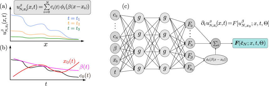
Figure 1: (a) A 1D example of the spectral expansion in an unbounded domain with scaling factor $\beta$ and displacement $x_{0}$ (Eq. (7)). (b) The evolution of the coefficient $c_{0}(t)$ and the two tuning parameters $\beta(t),x_{0}(t)$. (c) A schematic of how to reconstruct Eq. (1) satisfied by the spectral expansion approximation $u_{N,x_{0}}^{\beta}$. The time $t$, expansion coefficients $c_{i}$, and tuning variables $\beta(t)$, and $x_{0}$ are inputs of the neural network, which then outputs $\bm{F}(\tilde{\bm{c}}_{N};t,\Theta)=(F_{0},...,F_{N},F_{\beta},F_{x_{0}})$. The basis functions $\phi_{i}\big{(}\beta(t)(x-x_{0}(t))\big{)}$ are shaped by the time-dependent parameters which obey $\tfrac{\text{d}\beta}{\text{d}t}\approx F_{\beta}$ and $\tfrac{\text{d}x_{0}}{\text{d}t}\approx F_{x_{0}}$.

The spectral neural DE learning method proposed here differs substantially from the s-PINN framework because it does not make any assumption on the form of the spatiotemporal DE in Eq. (1) other than that the RHS $F$ does not contain time-differentials or time-integrals of $u(x,t)$. It inputs both the solution $u(x,t)$ (in terms of a spectral expansion) and $t$ into the neural network and applies a neural ODE model [16] (see Fig. 1 (c)). Thus, general DEs such as Eq. (1) can be learned with little knowledge of the RHS. To summarize, the proposed method presented in this paper

1. does not require assumptions on the $u$-dependence of $F$ other than it should not contain any time-derivatives or time-integrals of $u$. Both spatiotemporal PDEs and integro-differential equations can be learned in a unified way.

2. directly learns the dynamics of a spatiotemporal DE by using a parameterized neural network that can time-extrapolate the solutions, and

3. does not rely on spatial discretization and can thus learn unbounded-domain DEs. By using adaptive spectral representations, our neural DE learning method also learns the dynamics of the adaptive parameters adjusting the basis functions.

In the next section, we formulate our spectral neural DE learning method. In Section 3, we use our spectral neural DE method to learn the underlying dynamics of DEs, across both bounded and unbounded domains, by carrying out numerical experiments. Although our main focus is to address learning unbounded-domain DEs, we perform benchmarking comparisons with other recent machine-learning based PDE learning methods available for bounded-domain problems. Concluding remarks are given in Section 4. Additional numerical experiments and results are given in the Appendix. Below is a table of the notation used in this paper.

Table 1: Overview of variables. Definitions of the main variables and parameters used in this paper.

Symbol	Definition
$N$	spectral expansion order
$\Theta$	neural network hyperparameters
$\phi_{i}$	$i^{\rm th}$ order basis function in a spatial spectral expansion
$\beta(t)$	spatial scaling factor in basis functions: $\phi_{i}(\beta(x-x_{0}))$
$x_{0}(t)$	spatial translation in basis functions: $\phi_{i}(\beta(x-x_{0}))$
$u_{N,x_{0}}^{\beta}(x,t)$	order $N$ spectral expansion approximation:
	$u_{N,x_{0}}^{\beta}=\sum_{i=0}^{N}c_{i}^{\beta(t)}(t)\phi_{i}(\beta(x-x_{0}(t)))$
$\hat{\mathcal{H}}_{i}$	generalized Hermite function of order $i$

2 Spectral neural DE learning method

We now develop a spectral neural DE learning method for general spatiotemporal DEs of the general structure of Eq. (1), assuming the operator $F[u;x,t]$ does not involve time-differentiation or time-integration of $u(x,t)$. However, unlike in [5], the operator $F[u;x,t]$ can take any other form including differentiation in space, spatial convolution, and nonlinear terms.

First, consider a bounded spatial domain $\Omega$. Upon choosing proper orthogonal basis functions $\{\phi_{i}(x)\}_{i=0}^{N}$, we can approximate $u(x,t)$ by the spectral expansion in Eq. (2) and obtain ordinary equations of the coefficients $\bm{c}_{N}(t)\coloneqq(c_{0}(t),...,c_{N}(t))$ as Eq. (3). We aim to reconstruct the dynamics $F(\bm{c}_{N};t)$ in Eq. (3) by using a neural network

$$\bm{F}(\bm{c}_{N};t)\approx\bm{F}(\bm{c}_{N};t,\Theta),$$ (4)

where $\Theta$ is the set of parameters in the neural network. We can then construct the RHS of Eq. (1) using $F[u;x,t,\Theta]\approx\sum_{i=0}^{N}F_{i}(\bm{c}_{N};t,\Theta)\phi_{i}(x)$ where $F_{i}$ is the $i^{\text{th}}$ component of the vector $\bm{F}(\bm{c}_{N};t,\Theta)$. We shall use the neural ODE to learn the dynamics $\bm{F}(\bm{c}_{N};t,\Theta)$ by minimizing the mean loss function $L(u_{N}(x,t;\Theta),u(x,t))$ between the numerical solution $u_{N}(x,t;\Theta)$ and the observations $u(x,t)$. When data are provided at discrete time points $t_{j}$, we need to minimize

$$\sum_{m=1}^{M}\sum_{j=1}^{T}L\big{(}u_{N,m}(x,t_{j};\Theta),u_{m}(x,t_{j})\big{)},$$ (5)

with respect to $\Theta$. Here, $u_{m}(x,t_{j})$ is the solution at $t_{j}$ of the $m^{\text{th}}$ trajectory in the dataset and $u_{N,m}(x,t_{j};{\Theta})$ denotes the spectral expansion solution reconstructed from the coefficients $\bm{c}_{N,m}$ obtained by the neural ODE of the $m^{\text{th}}$ sample at $t_{j}$.

To solve unbounded domain DEs in $\Omega\subseteq\mathbb{R}^{D}$, two additional parameters are needed to scale and translate the spatial argument $\bm{x}$, a scaling factor $\bm{\beta}\coloneqq(\beta^{1},\ldots,\beta^{D})\in\mathbb{R}^{D}$, and a shift factor $\bm{x}_{0}\coloneqq(x_{0}^{1},\ldots,x_{0}^{D})\in\mathbb{R}^{D}$. These factors, particularly in unbounded domains, often need to be dynamically adjusted to obtain accurate spectral approximations of the original function [17, 6, 18]. Note that given the observed $u(X,t)$, the ground truth coefficients $c_{i}(t)$ as well as the spectral adjustment parameters $\beta(t)$ and $x_{0}(t)$ are obtained by minimizing the frequency indicator (introduced in [6])

$$\mathcal{F}(u;\beta,x_{0})=\sqrt{\frac{\sum_{i=N-[\tfrac{N}{3}]+1}^{N}c_{i}^{2}}{\sum_{i=0}^{N}c_{i}^{2}}}$$ (6)

that measures the error in the numerical representation of the solution $u$ [19]. Therefore, minimizing $\mathcal{F}(u;\beta,x_{0})$ will also minimize the approximation error $\|u-\sum_{i=0}^{N}c_{i}\hat{\mathcal{H}}(\beta(t)(x-x_{0}(t)))\|^{2}_{2}$.

Generalizing the spectral approximation Eq. (2) to higher spatial dimensions, we can write

$$u(\bm{x},t)\approx u_{N,\bm{x}_{0}}^{\bm{\beta}}(\bm{x},t)=\sum_{i=0}^{N}c_{i}(t)\phi_{i}\big{(}\bm{\beta}*(\bm{x}-\bm{x}_{0})\big{)},$$ (7)

where $\bm{\beta}*(\bm{x}-\bm{x}_{0})\coloneqq(\beta^{1}(x-x_{0}^{1}),...,\beta^{D}(x-x_{0}^{D}))$ is the Hadamard product.

The two parameters $\bm{\beta}(t),\bm{x}_{0}(t)$, which are also functions of time, can also be learned by the neural ODE. More specifically, we append the scale and displacement variables to the coefficient vector $\bm{c}_{N}(t)$ and write $\tfrac{\mbox{d}\tilde{\bm{c}}_{N}}{\mbox{d}t}=\bm{F}(\tilde{\bm{c}}_{N};t)$ for the ODEs satisfied by $\tilde{\bm{c}}_{N}\coloneqq\big{(}c_{0}(t),...,c_{N}(t),\bm{\beta}(t),\bm{x}_{0}(t)\big{)}$. The underlying dynamics $\bm{F}(\tilde{\bm{c}}_{N};t)$ is approximated as

$$\bm{F}(\tilde{\bm{c}}_{N};t)\approx\bm{F}(\tilde{\bm{c}}_{N};t,\Theta)$$ (8)

by minimizing with respect to $\Theta$ a loss function that also penalizes the error in $\beta$ and $x_{0}$

$$\sum_{m=1}^{M}\sum_{j=1}^{T}\bigg{[}L\big{(}u_{N,\bm{x}_{0,m},m}^{\bm{\beta}_{m}}(\bm{x},t_{j};{\Theta}),u_{m}(\bm{x},t_{j})\big{)}$$ (9)

$$\hskip 105.2751pt+\lambda\|\bm{\beta}_{m}(t_{j})-\bm{\beta}_{m}(t_{j};\Theta)\|_{2}^{2}+\lambda\|\bm{x}_{0,m}(t_{j})-\bm{x}_{0,m}(t_{j};\Theta)\|_{2}^{2}\bigg{]}.$$

Similarly, the DE satisfied by $u_{N,\bm{x}_{0}}^{\bm{\beta}}(\bm{x},t)$ is

$$\partial_{t}u_{N,\bm{x}_{0}}^{\bm{\beta}}(\bm{x},t)=F[u_{N,\bm{x}_{0}}^{\bm{\beta}};\bm{x},t,\Theta],$$ (10)

where

$$F[u_{N,\bm{x}_{0}}^{\bm{\beta}};\bm{x},t,\Theta]=\sum_{i=0}^{N}F_{i}(\tilde{\bm{c}}_{N};t,\Theta)\phi_{i}(\bm{\beta}(\bm{x}-\bm{x}_{0}))$$ (11)

and $F_{i}$ is the $i^{\text{th}}$ component of $\bm{F}(\tilde{\bm{c}}_{N};t,\Theta)$.

Here, $\bm{\beta}_{m}(t_{j})$ and $\bm{x}_{0,m}(t_{j})$ are the scaling factor and the displacement of the $m^{\text{th}}$ sample at time $t_{j}$, respectively, and $\lambda$ is the penalty due to squared mismatches in the scaling and shift parameters $\beta$ and $x_{0}$. In this way, the dynamics of the variables $\bm{x}_{0},\bm{\beta}$ are also learned by the neural ODE so they do not need to be manually adjusted as they were in [19, 6, 18, 15].

In case the space $\Omega$ is high-dimensional, and the solutions are sufficiently smooth and well-behaved, they can be approximated by restricting the basis functions $\{\phi_{i,x_{0}}^{\beta}\}$ to those in the hyperbolic cross space of the full tensor product of basis functions. If this projection is performed optimally, the effective dimensionality of the problem can be reduced [20, 21] without significant loss of accuracy. We will show that our method can also easily incorporate hyperbolic spaces to enhance training efficiency in modestly higher-dimensional problems.

3 Numerical experiments

Here, we carry out numerical experiments to test our spectral neural DE method by learning the underlying DE given data in both bounded and unbounded domains. In this section, all numerical experiments are performed using the odeint_adjoint function along with the dopri5 numerical integration method developed in [16] for training the neural network. Both stochastic gradient descent (SGD) and the Adam method are used to optimize parameters of the neural network. In this work, we set $L(\cdot,\cdot)$ to be the relative squared $L^{2}$ error

$$L(u(x,t_{i}),u_{N}(x,t_{i};\Theta))\coloneqq\frac{\|u(x,t_{i})-u_{N}(x,t_{i};\Theta)\|_{2}^{2}}{\|u\|_{2}^{2}}$$ (12)

in the loss function Eq. (5) used for training.

Since algorithms already exist for learning bounded-domain PDEs, we we first examine a bounded-domain problem in order to benchmark our spectral neural DE method against two other recent representative methods, a convolutional neural PDE learner [5] and a Fourier neural operator PDE learning method [13].

Example 1.

For our first test example, we consider learning a bounded-domain Burgers’ equation that might be used to describe the behavior of viscous fluid flow [22]:

$$\partial_{t}u+\tfrac{1}{2}\partial_{x}(u^{2})= \tfrac{1}{10}\partial_{xx}u,\quad x\in(-1,1),\,\,t\geq 0,$$ (13)

$$u(-1,t)=u(1,t),\,\,\partial_{x}u(-1,t) =\partial_{x}u(1,t),\,\,\,u(x,0)=-\frac{1}{5}\frac{\phi_{x}(x,0)}{\phi(x,0)},$$

where

$$\phi(x,t)\equiv 5+\frac{2+\xi_{1}}{2}e^{-\pi^{2}t/10}\sin\pi x+\frac{\xi_{2}}{2}e^{-2\pi^{2}t/5}\cos 2\pi x.$$ (14)

This model admits the analytic solution $u(x,t)=-{\phi_{x}(x,t)}{5\phi(x,t)}$. We then sample the two independent random variables from $\xi_{1},\xi_{2}\sim\mathcal{U}(0,1)$ to generate a class of solutions to Eq. (14) $\{u\}_{\xi_{1},\xi_{2}}$ for both training and testing. To approximate $F$ in Eq. (4), we use a neural network that has one intermediate layer with 300 neurons and the ELU activation function. The basis functions in Eq. (2) are taken to be Chebyshev polynomials. For training, we use two hundred solutions (each corresponding to a pair of values $(\xi_{1},\xi_{2})$ of Eq. (13), record the expansion coefficients $\{c_{i}\}_{i=0}^{9}$ at different times $t_{j}=j\Delta{t},\Delta{t}=\frac{1}{4},j=0,\ldots,4$. The test set consists of another $100$ solutions, also evaluated at times $t_{j}=j\Delta{t},\Delta{t}=\frac{1}{4},j=0,\ldots,4$.

In this bounded-domain problem, we can compare our results with those generated from the Fourier neural operator (FNO) and the convolutional neural PDE learner methods. In the FNO method, four intermediate Fourier convolution layers with 128 neurons in each layer were used to input the initial condition $u(i\Delta x,0)$ and function values $u(i\Delta x,t=j\Delta t)$ (with $\Delta x=\frac{1}{128},\Delta t=\frac{1}{4}$) [13]. In the convolutional neural PDE learner comparison, we used seven convolutional layers with 40 neurons in each layer to input $u(i\Delta x,j\Delta t)$ (with $\Delta{x}=\frac{1}{100},\Delta{t}=\frac{1}{250}$) [5]. Small $\Delta{x}$ and $\Delta{t}$ were used in the convolutional neural PDE learner method because this method depends on both spatial and temporal discretization, requiring fine discretization in both dimensions. For all three methods, we used the Adam method to perform gradient descent with a learning rate $\eta=0.001$ to run 10000 epochs, which was sufficient for the errors in all three methods to converge. We list in Table 2 both the MSE error $\frac{1}{TM}\sum_{m=1}^{M}\sum_{j=1}^{T}\|u_{N,m}(x,t_{j};\Theta)-u_{m}(x,t_{j})\|_{2}^{2}$ and the mean relative $L^{2}$ error

$$\frac{1}{TM}\sum_{m=1}^{N}\sum_{j=1}^{T}\frac{\|u_{N,m}(x,t_{j};\Theta)-u_{m}(x,t_{j})\|_{2}}{\|u_{m}(x,t_{j})\|_{2}}.$$ (15)

Table 2: Comparison of different PDE learners. The convolutional PDE learner, the Fourier neural operator method, and our proposed spectral neural PDE learner are used to learn the dynamics of Burgers’ equation Eq. (13) in a bounded domain. The FNO method gives the best performance and the convolutional neural PDE performs the worst. Our proposed spectral neural PDE learner achieves performance comparable to the FNO method.

	Training error		Testing error
	MSE	Mean relative $L^{2}$	MSE	Mean relative $L^{2}$
convolutional	2.39e-05$\pm$1.82e-05	1.68e-02$\pm$7.86e-03	1.10e-04$\pm$6.62e-05	2.82e-02$\pm$6.62e-03
Fourier	3.21e-07$\pm$1.53e-07	7.43e-03$\pm$1.76e-03	4.66e-07$\pm$3.43e-07	8.61e-03$\pm$2.86e-03
spectral	1.15e-06$\pm$9.72e-07	9.82e-03$\pm$4.95e-03	1.17e-06$\pm$9.73e-07	9.99e-03$\pm$4.97e-03

For the FNO and spectral PDE learning methods, we aim to minimize the relative squared loss $L^{2}$ (Eq. (12)), while for the convolution neural PDE method, we must minimize the MSE loss since only partial and local spatial information on the solution is inputted during each training epoch so we cannot properly define a relative squared loss. Thus, as shown in Table 2, the MSE of the FNO method is smaller than the MSEs of the other two methods on the training set while the convolutional neural PDE method performs the worst. Nonetheless, our proposed neural spectral PDE learning approach gives similar performance compared to the FNO method, providing comparable mean relative $L^{2}$ and MSE errors for learning the dynamics associated with the bounded-domain Burgers’ equation.

Additionally, the run times in this example were $2$ hours for the convolutional PDE learning method, 6 hours for the FNO method, and 5 hours for our proposed spectral neural DE learning approach. These computations were implemented on a 4-core Intel^® i7-8550U CPU, 1.80 GHz laptop using Python 3.8.10, Torch 1.12.1, and Torchdiffeq 0.2.3. Overall, even in bounded domains, our proposed spectral neural DE learning approach compares well with the recently developed convolutional neural PDE and FNO methods, providing comparable errors and efficiency in learning the dynamics of Eq. (13).

The Fourier neural operator method works well in reconstructing the Burgers’ equation in Example 1, and there could be other even more efficient methods for reconstructing bounded domain spatiotemporal DEs. However, reconstructing unbounded domain spatiotemporal DEs is substantially different from reconstructing bounded domain counterparts. First, discretizing space cannot be directly applied to unbounded domains; second, if we truncate an unbounded domain into a bounded domain, appropriate artificial boundary conditions need to be imposed [23]. Constructing such boundary conditions is usually complex and improper boundary conditions can lead to large errors, resulting erroneous learning of the DE. A simple example of when the FNO will fail when we truncate the unbounded domain into a bounded domain is provided in  A.

Since our spectral method uses basis functions, it obviates the need for spatial discretization and can be used to reconstruct unbounded-domain DEs. Dynamics in unbounded domains are intrinsically different from their bounded-domain counterparts because functions can display diffusive and convective behavior leading to, e.g., time-dependent growth at large $x$. This growth poses intrinsic numerical challenges when using prevailing finite element/finite difference methods that truncate the domain.

Although it is difficult for most existing methods to learn the dynamics in unbounded spatial domains, our spectral approach can reconstruct unbounded-domain DEs by simultaneously learning the expansion coefficients and the evolution of the basis functions. To illustrate this, we next consider a one-dimensional unbounded domain inverse problem.

Example 2.

Consider learning the solution

$$u(x,t;\xi_{1},\xi_{2},\xi_{3})=\frac{\xi_{1}}{\sqrt{t+1+\xi_{2}}}\exp\left[-\frac{(x-t-\xi_{3})^{2}}{t+1+\xi_{2}}\right],\,\,x\in\mathbb{R},\,t\in[0,1]$$ (16)

and its associated parabolic PDE

$$\partial_{t}u=-\partial_{x}u+\frac{1}{4}\partial_{xx}u,\quad u(x,0)=\frac{\xi_{1}}{\sqrt{1+\xi_{2}}}\exp\left[-\frac{(x-\xi_{3})^{2}}{\xi_{2}+1}\right].$$ (17)

This problem is defined on an unbounded domain and thus neither the FNO nor the convolutional neural PDE methods can be used as they rely on spatial discretization (and thus bounded domains). However, given observational data $u(\cdot,t)$ for different $t$, we can calculate the spectral expansion of $u$ via the generalized Hermite functions [8]

$$u(x,t)\approx u_{N,x_{0}}^{\beta}=\sum_{i=0}^{N}c_{i}(t)\hat{\mathcal{H}}_{i}\big{(}\beta(t)(x-x_{0}(t))\big{)}$$ (18)

and then use the spectral neural DE learning approach to reconstruct the dynamics $F$ in Eq. (1) satisfied by $u$. Recall that the scaling factor $\beta(t)$ and the displacement of the basis functions $x_{0}(t)$ are also to be learned. To penalize misalignment of the spectral expansion coefficients and the scaling and displacement factors $\beta$ and $x_{0}$, we use the loss function Eq. (9). Note that taking the derivative of $\beta(t_{j};\Theta)$ with respect to $\Theta$ in the first term of Eq. (9) would involve evaluating  $\int\partial_{\Theta}\beta(t_{j};\Theta)(x-x_{0}(t_{j};\Theta))u_{N,x_{0}}^{\beta}(t_{j};\Theta)\cdot\partial_{x}u_{N,x_{0}}^{\beta}(x,t_{j};\Theta)\text{d}{x}$; similarly, taking the derivative of $x_{0}(t_{j};\Theta)$ with respect to $\Theta$ would involve evaluating $\int\partial_{\Theta}x_{0}(t_{j};\Theta)\beta(t_{j};\Theta)u_{N,x_{0}}^{\beta}(t_{j};\Theta)\partial_{x}u_{N,x_{0}}^{\beta}(x,t_{j};\Theta)\text{d}{x}$. Expressing $\partial_{x}u_{N,x_{0}}^{\beta}(x,t_{j};\Theta)$ in terms of the basis functions $\phi_{i,x_{0}}^{\beta}$ would involve a dense matrix-vector multiplication of the coefficients of the expansion $\partial_{x}u_{N,x_{0}}^{\beta}(x,t_{j};\Theta)$, which might be computationally expensive during backward propagation in the stochastic gradient descent (SGD) procedure. Alternatively, suppose the parameter set of the neural network is $\Theta_{j-1}$ before the $j^{\text{th}}$ training epoch. We can fix $\tilde{\beta}(t_{j})\coloneqq\beta(t_{j};\Theta_{j-1}),\tilde{x}_{0}(t_{j})\coloneqq x_{0}(t_{j};\Theta_{j-1})$ ($\tilde{\beta},\tilde{x}_{0}$ are fixed values and do not depend on the weights $\Theta$) and then modify Eq. (9) to

$$\sum_{m=1}^{M}\sum_{j=1}^{T}\bigg{[}\frac{\|u_{N,\tilde{x}_{0,m}(t_{j})}^{\tilde{\beta}_{m}(t_{j})}(x,t_{j};\Theta)-u_{m}(x,t_{j})\|_{2}^{2}}{\|u_{m}(x,t_{j})\|_{2}^{2}}$$ (19)

$$\hskip 102.43008pt+\lambda\big{(}\beta_{m}(t_{j};\Theta)-\beta_{m}(t_{j})\big{)}^{2}+\lambda\big{(}x_{0,m}(t_{j};\Theta)-x_{0,m}(t_{j})\big{)}^{2}\bigg{]},$$

so that backpropagation within each epoch will not involve taking derivatives w.r.t. $\Theta$ for $\tilde{\beta}_{m}(t_{j}),\tilde{x}_{0,m}(t_{j})$ in the first term of Eq. (19). The reason is that when $\beta_{m}(t),x_{m,0}(t)$ are well fitted (e.g. $\beta_{m}(t;\Theta_{j-1})=\beta(t),x_{m,0}(t;\Theta_{j-1})=x_{0}(t)$ are ground-truth values), Eq. (19) will simply become

$$\sum_{m=1}^{M}\sum_{j=1}^{T}\frac{\|u_{N,\tilde{x}_{0,m}(t_{j})}^{\tilde{\beta}_{m}(t_{j})}(x,t_{j};\Theta)-u_{m}(x,t_{j})\|_{2}^{2}}{\|u_{m}(x,t_{j})\|_{2}^{2}}=\sum_{m=1}^{M}\sum_{j=1}^{T}\frac{\sum_{i=0}^{N}(c_{m,i}(t_{j};\Theta)-c_{i}(t_{j}))^{2}}{\sum_{i=0}^{N}c_{m,i}(t_{j})^{2}}$$ (20)

so no derivative of $\beta,x_{0}$ w.r.t. $\Theta$ will be used and only the gradient of $F$ in Eq. (4) w.r.t. $\Theta$ arises. Therefore, we can consider separating the fitting of the coefficients $c_{i}(t)$ and the fitting of $\beta(t),x_{0}(t)$.

We use 100 samples for training and another 50 samples for testing with $N=9,\Delta{t}=0.1,T=9,\lambda=0.1$. A neural network with two hidden layers, 200 neurons in each layer, and the ELU activation function is used for training. Both training and testing data are taken from Eq. (16) with sampled parameters $\xi_{1}\sim\mathcal{N}(3,\tfrac{1}{4}),\,\,\xi_{2}\sim\mathcal{U}(0,\tfrac{1}{2}),\,\,\xi_{3}\sim\mathcal{N}(0,\tfrac{1}{2})$.

Setting $\lambda=0.1$, we first compare the two different loss functions Eqs. (9) and (19). After running 10 independent training processes using SGD, each containing 2000 epochs and using learning rate $\eta=0.0002$, the average relative $L^{2}$ error when using the loss function Eq. (9) are larger than the average relative $L^{2}$ errors when using the loss function Eq. (19). This difference arises in both the training and testing sets as shown in Fig. 2(a).

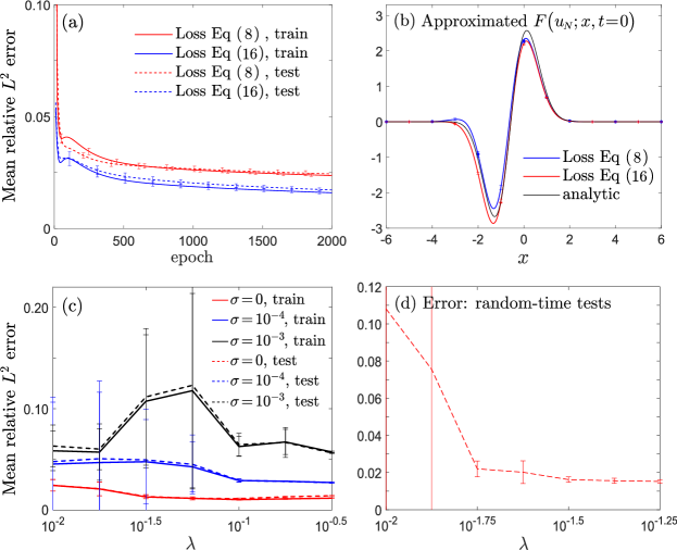
Figure 2: (a) Errors using different loss functions Eqs. (9) and (19). (b) Average dynamics found from using Eqs. (9) and (19). (c) Errors with $\lambda$ and $\sigma$. (d) Errors on the testing set with random times $t_{i}\sim\mathcal{U}(0,1.5)$.

In Fig. 2(b), we plot the average learned $F$ (RHS in Eq. (1)) for a randomly select sample at $t=0$ in the testing set. The dynamics learned by using Eq. (19) is a little more accurate than that learned by using Eq. (9). Also, using the loss function Eq. (19) required only $~{}\sim 1$ hour of computational time compared to 5 days when learning with Eq. (9) (on the 4-core i7-8550U laptop). Therefore, for efficiency and accuracy, we adopt the revised loss function Eq. (19) and separately fit the dynamics of the adaptive spectral parameters ($\beta,x_{0}$) and the spectral coefficients $c_{i}$.

We also explore how network architecture and regularization affect the reconstructed dynamics. The results are shown in  B, from which we observe that a wider and shallower neural network with 2 or 4 intermediate layers and 200 neurons in each layer yields the smallest errors on both the training and testing sets, and short run times. We also apply a ResNet [24] as well as dropout [25, 26] to regularize the neural network structure. Dropout regularization does not reduce either the training error or the testing error probably because even with a feedforward neural network, the errors from our spectral neural DE learner on the training set are close to those on the testing set and there is no overfitting issue. On the other hand, applying the ResNet technique leads to about a  20% decrease in errors. Results from using ResNets and dropout are shown in  B.

Next, we investigate how noise in the observed data and changes in the adaptive parameter penalty coefficient $\lambda$ in Eq. (19) impact the results. Noise is incorporated into simulated observational data as

$$u_{\xi}(x,t)=u(x,t)[1+\xi(x,t)],$$ (21)

where $u(x,t)$ is the solution to the parabolic equation Eq. (17) given by Eq. (16) and $\xi(x,t)\sim\mathcal{N}(0,\sigma^{2})$ is a Gaussian-distributed noise that is both spatially and temporally uncorrelated (i.e., $\langle\xi(x,t)\xi(t,s)\rangle=\sigma^{2}\delta_{x,y}\delta_{s,t}$). The noise term is assumed to be independent for different samples. We use a neural network with 2 hidden layers, 200 neurons in each layer, to implement 10 independent training processes using SGD and a learning rate $\eta=0.0002$, each containing 5000 epochs. Results are shown in Fig. 2(c) and further tabulated in C. For $\sigma=0$, choosing an intermediate $\lambda\in(10^{-1.5},10^{-1}]$ leads the smallest errors and an optimal balance between learning the coefficients $c_{i}$ and learning the dynamics of $\beta,x_{0}$. When $\sigma$ is increased to nonzero values ($\sim 10^{-4}-10^{-3}$), a larger $\lambda\sim 10^{-0.75}-10^{-0.5}$ is needed to keep errors small (see Fig. 2(c) and C). If the noise is further increased to, say, $\sigma=10^{-2}$ (not shown in Fig. 2), an even larger $\lambda\sim 10^{-0.5}$ is needed for training to converge. This behavior arises because the independent noise $\xi(x,t)\sim\mathcal{N}(0,\sigma^{2})$ contributes more to high-frequency components in the spectral expansion. In order for training to converge, fitting the shape of the basis functions by learning $\beta,x_{0}$ is more important than fitting noisy high-frequency components via learning $c_{i}$. A larger $\lambda$ puts more weight on learning the dynamics of $\beta,x_{0}$ and basis function shapes.

We also investigate how the intrinsic noise in the parameters $\xi_{1},\xi_{2},\xi_{3}$ of the solution’s distribution Eq. (16) affect the accuracy of the learned DE by our method. We found that if the intrinsic noise in $\xi_{1},\xi_{2},\xi_{3}$ is larger, then the training errors of the learned DE models are larger. However, compared to models trained on data with lower $\xi_{1},\xi_{2},\xi_{3}$, training using noisier data leads to lower errors when testing data are also noisy. Training with noisier data leads to better performance when testing data are also noisy. The training and testing errors that show this feature are presented in D.

Finally, we test whether the parameterized $F$ (Eq. (8)) learned from the training set can extrapolate well beyond the training set sampling interval $t\in[0,0.9]$. To do this, we generate another 50 trajectories and sample each of then at random times $t_{i}\sim\mathcal{U}(0,1.5),i=1,...,9$. We then used models trained with $\sigma=0$ and different $\lambda$ to test. As shown in Fig. 2(d), our spectral neural DE learner can accurately extrapolate the solution to times beyond the training set sampling time intervals. We also observe that a stronger penalty on $\beta$ and $x_{0}$ ($\lambda=10^{-0.5}$) leads to better extrapolation results.

In the last example, we carry out a numerical experiment on learning the evolution of a Gaussian wave packet (which may depend on nonlocal interactions) across a two-dimensional unbounded domain $(x,k)\in\mathbb{R}^{2}$. We use this case to explore improving training efficiency by using a hyperbolic cross space to reduce the number of coefficients in multidimensional problems.

Example 3.

We solve a 2D unbounded-domain problem of fitting a Gaussian wave packet’s evolution

$$f(x,k,t;\xi_{1},\xi_{2})=2e^{-\frac{(x-\xi_{1})^{2}}{2a^{2}}}\,e^{2\beta t(x-\xi_{1})(k-\xi_{2})}\,e^{-2a^{2}(1+\beta^{2}t^{2})(k-\xi_{2})^{2}},$$ (22)

where $\xi_{1}$ is the center of the wave packet and $a$ is the minimum positional spread. If $\xi_{2}=0$, the Gaussian wave packets defined in Eq. (22) solves the stationary zero-potential Wigner equation, an equation often used in quantum mechanics to describe the evolution of the Wigner quasi-distribution function [27, 28]. We set $a=1$ and $\beta=1/2$ in Eq. (22) and independently sample $\xi_{1},\xi_{2}\sim\mathcal{U}(-1/2,1/2)$ to generate data. Thus, the DE satisfied by the highly nonlinear Eq. (22) is unknown and potentially involves nonlocal convolution terms. In fact, there could be infinitely many DEs, including complicated nonlocal DEs, that can describe the dynamics of Eq. (22). An example of such a nonlocal DE is

$$\partial_{t}f+ 2a^{2}\beta A[f;x,k,t]\partial_{x}f(x,k,t)=0,$$ (23)

$$A[f;x,k,t] =\frac{\beta t(x-B[f;x,k,t])}{2a^{2}(1+\beta^{2}t^{2})}+\sqrt{\tfrac{\log D[f;k,t]-C(t)-\log(f/2)}{a^{2}(1+\beta^{2}t^{2})}},$$

$$B[f;x,k,t] =x-\sqrt{2a^{2}(1+\beta^{2}t^{2})}\times\sqrt{2C(t)-2\log D[f;x,k,t]+\log(f/2)},$$

$$C(t) =\tfrac{1}{2}\log\left[\frac{\pi}{a^{2}(1+\beta^{2}t^{2})}\right],$$

$$D[f;x,k,t] =\int f(x,y,t)e^{-2a^{2}(1+\beta^{2}t^{2})(y-k)^{2}}\text{d}y.$$

We wish to learn the underlying dynamics using a parameterized $F$ in Eq. (8). Since the Gaussian wave packet Eq. (22) is defined in the unbounded domain $\mathbb{R}^{2}$, learning its evolution requires information over the entire domain. Thus, methods that depend on discretization of space are not applicable.

Our numerical experiment uses Eq. (22) as both training and testing data. We take $\Delta{t}=0.1,t_{j}=j\Delta{t},j=0,...,10$ and generate 100 trajectories for training. For this example, training with ResNet results in diverging gradients, whereas the use of a feedforward neural network yields convergent results. So we use a feedforward neural network with two hidden layers and 200 neurons in each hidden layer and the ELU activation function. We train across 1000 epochs using SGD with momentum (SGDM), a learning rate $\eta=0.001$, $\text{momentum}=0.9$, and $\text{weight decay}=0.005$. For testing, we generate another 50 trajectories, each with starting time $t_{0}=0$ but $t_{j}$ taken from $\mathcal{U}(0,1),j=1,\dots,10$. We use the spectral expansion

$$f_{N}(x,k,t_{j};\xi_{1},\xi_{2})=\sum_{i=0}^{14}\sum_{\ell=0}^{14}c_{i,\ell}(t_{j})\hat{\mathcal{H}}_{i}(\beta^{1}(x-x_{0}^{1}))\hat{\mathcal{H}}_{\ell}(\beta^{2}(k-k_{0}^{2}))$$ (24)

to approximate Eq. (22). We record the coefficients $c_{i,\ell}$ as well as the scaling factors and displacements $\beta^{1},\beta^{2},x_{0}^{1},k_{0}^{2}$ at different $t_{j}$.

Because $(x,k)\in\mathbb{R}^{2}$ are defined in a 2-dimensional space, instead of a tensor product, we can use a hyperbolic cross space for the spectral expansion to effectively reduce the total number of basis functions while preserving accuracy [20]. Similar to the use of sparse grids in the finite element method [29, 30], choosing basis functions in the space

$$V_{N,\gamma}^{\vec{\beta},\vec{x}_{0}}\coloneqq\text{span}\Big{\{}\hat{\mathcal{H}}_{n_{1}}(\beta^{1}(x-x_{0}^{1}))\hat{\mathcal{H}}_{n_{2}}(\beta^{2}(k-k_{0}^{2})):|\vec{n}|_{\text{mix}}\|\vec{n}\|_{\infty}^{-\gamma}\leq N^{1-\gamma}\Big{\}},$$ (25)

$$\vec{n}\coloneqq(n_{1},n_{2}),~{}|\vec{n}|_{\text{mix}}\coloneqq\max\{n_{1},1\}\cdot\max\{n_{2},1\}$$

can reduce the effective dimensionality of the problem. We explored different hyperbolic spaces $V_{N,\gamma}^{\vec{\beta},\vec{x}_{0}}$ with different $N$ and $\gamma$. We use the loss function Eq. (19) with $\lambda=\tfrac{1}{50}$ for training. The results are listed in E. To show how the loss function Eq. (19) depends on the coefficients $c_{i,\ell}$ in Eq. (24), we plot saliency maps [31] for the quantity $\tfrac{1}{10}\sum_{j=1}^{10}\big{|}\frac{\partial\text{Loss}_{j}}{\partial c_{i,\ell}(0)}\big{|}$, the absolute value of the partial derivative of the loss function Eq. (19) w.r.t. $c_{i,\ell}$ averaged over 10 training processes.

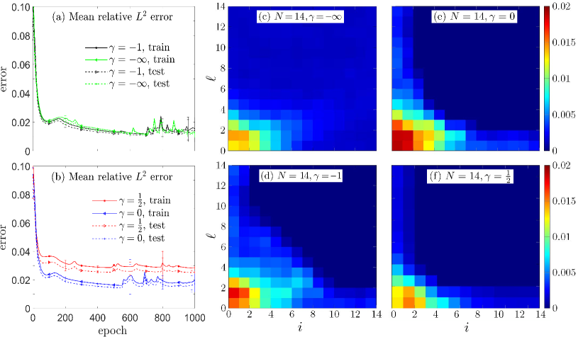
Figure 3: (a,b) Mean relative $L^{2}$ errors for $N=14$ and $\gamma=-\infty,-1,0,1/2$. (c-f) Saliency maps showing the mean absolute values of the partial derivative of the loss function w.r.t. to $\{c_{i,\ell}(0)\}$ for $\gamma=-\infty,-1,0,1/2$.

As shown in Fig. 3(a,b), using $\gamma=-1,0$ leads to similar errors as the full tensor product $\gamma=-\infty$, but could greatly reduce the number of coefficients and improve training efficiency. Taking a too large $\gamma=1/2$ leads to larger errors because useful coefficients are left out. From Fig. 3(c-f), there is a resolution-invariance for the dependence of the loss function on the coefficients $c_{i,\ell}$ though using different hyperbolic spaces with different $\gamma$. We find that an intermediate $\gamma\in(-\infty,1)$ (e.g., $\gamma=-1,0$) can be used to maintain accuracy and reduce the number of inputs/outputs when reconstructing the dynamics of Eq. (22). Overall, the “curse of dimensionality” can be mitigated by adopting a hyperbolic space for the spectral representation.

Finally, in F, we consider source reconstruction in a heat equation. Our proposed spectral neural DE learning method achieves an average relative error $L^{2}\approx 0.1$. On the other hand, if all terms on the RHS of Eq. (1) except an unknown source (which does not depend on the solution) is known, the recently developed s-PINN method [15] achieves a higher accuracy. However, if in addition to the source term, additional terms on on the RHS of Eq. (1) are unknown, s-PINNs cannot be used but our proposed spectral neural DE learning method remains applicable.

4 Conclusion

In this paper, we proposed a novel spectral neural DE learning method that is suitable for learning spatiotemporal DEs from spectral expansion data of the underlying solution. Its main advantages is that it can be applied to learning both spatiotemporal PDEs and integro-differential equations in unbounded domains, while matching the performance of the most recent high-accuracy PDE learning methods applicable to only bounded domains. Moreover, our proposed method has the potential to deal with higher-dimensional problems if a proper hyperbolic cross space can be justified to effectively reduce the dimensionality.

As a future direction, we plan to apply our spectral neural DE learning method to many other inverse-type problems in physics. One possible application is to learn the stochastic dynamics associated with anomalous transport [32] in an unbounded domain, which could be associated with fractional derivative or integral operators in the corresponding $F[u;x,t]$ term. Finally, since the number of inputs (expansion coefficients) grows exponentially with spatial dimension, very high dimensional problems may not be sufficiently mitigated by even the most optimal cross space hyperbolicity $\gamma$ (see Eq. (25)). Thus, higher dimensional problems remain challenging and exploring how prior knowledge on the observed data can be used within our spectral framework to address them may be a fruitful avenue of future investigation.

Appendix A Using Fourier neural operator to reconstruct unbounded domain DEs

We shall show through a simple example that it is usually difficult to apply bounded domain DE reconstructing methods to reconstruct unbounded domain DEs even if we truncate the unbounded domain into a bounded domain, because appropriate boundary conditions must be provided. We wish to use the Fourier neural operator method to reconstruct the unbounded domain DE

$$u_{t}=\frac{1}{4}u_{xx},\quad x\in\mathbb{R},\,\,t\in[0,1].$$ (26)

If one imposes the initial condition $u(x,0)=10\xi\exp(-100x^{2})$, then

$$u(x,t)=\frac{\xi}{\sqrt{0.01+t}}\exp(-\tfrac{x^{2}}{0.01+t})$$ (27)

is the analytic solution to Eq. (26). For this problem, we will assume $\xi\sim\mathcal{U}(1,\frac{3}{2})$.

Since the Fourier neural operator (FNO) method relies on spatial discretization and grids, and cannot be directly applied to unbounded domain problems, we truncate the unbounded domain. Suppose one is interested in the solution’s behavior for $x\in[-1,1]$. One approach is to truncate the unbounded domain $x\in\mathbb{R}$ to $[-1,1]$ and use the FNO method to reconstruct the solution $u(x,t),\,x\in[-1,1],t\in[0,1]$ given $u(x,0)$. However, we show how improper boundary conditions of the truncated domain can leads to large errors.

For example, we assume the training set satisfies the boundary condition $u(x=\pm 1,t)=0$, which is not the correct boundary condition since it is inconsistent with the ground truth solution. Therefore, we will not be reconstructing the model in Eq. (26). We generated the testing dataset using the correct initial condition $u(x,0)=10\xi\exp(-100x^{2})$, without boundary conditions. The results are given in Table 3.

Table 3: Training and testing errors when using the FNO method and truncating the unbounded domain. However, an incorrect boundary condition for the training set is imposed. The error is significantly larger on the testing set than that on the training set because a different DE is reconstructed from the training data.

	Training error		Testing error
	​​MSE​​	​​Mean relative $L^{2}$​​	​​MSE	Mean relative $L^{2}$ ​​
Fourier	3.78e-05 $\pm$ 1.78e-05	6.09e-03$\pm$1.47e-03	8.95e-04$\pm$6.95e-05	3.07e-02$\pm$1.17e-03

From Table 3, the testing error is significantly larger than the training error because a different DE (not Eq. (26)) is constructed from the training data, which is not the heat equation we expect. Therefore, even if methods such FNO are efficient in bounded domain DE reconstruction problems, directly using them to reconstruct unbounded domain problems is not feasible if we cannot construct appropriate boundary conditions.

Appendix B Dependence on neural network architecture

The neural network structure of the parameterized $F[u;x,t,\Theta]$ may impact learned dynamics. To investigate how the neural network structure influences results, we use neural networks with various configurations to learn the dynamics of Eq. (16) in Example 2 in the noise-free limit. We set the learning rate $\eta=0.0002$ and apply networks with 2,3,5,8 intermediate layers, and 50, 80, 120, 200 neurons in each layer.

Table 4: The relative $L^{2}$ errors on the training set and testing set (in parentheses) for Example 2 when there is no noise in both the training data and the testing data ($\sigma=0$). $\lambda=0.1$ in Eq. (19), and the training rate is set to be $\eta=0.0005$ for 5000 training epochs using SGD.

	2	3	5	8
50	$0.0166$ $(0.0179)$	$0.0175$ $(0.0196)$	$0.0219$ $(0.0251)$	$0.0249$ $(0.0272)$
80	$0.0143$ $(0.0155)$	$0.0164$ $(0.0181)$	$0.0186$ $(0.0208)$	$0.0238$ $(0.0266)$
120	$0.0130$ $(0.0141)$	$0.0148$ $(0.0162)$	$0.0192$ $(0.0218)$	$0.0232$ $(0.0265)$
200	$0.0098$ $(0.0108)$	$0.0126$ $(0.0137)$	$0.0176$ $(0.0196)$	$0.0228$ $(0.0263)$

Table 5: The training time (in seconds) for Example 2 when there is no noise in both the training data and the testing data ($\sigma=0$). $\lambda=0.1$ in Eq. (19), and the training rate is set to be $\eta=0.0005$ for 5000 training epochs using SGD. Training was performed on a laptop with a 4-core Intel^® i7-8550U CPU @ 1.80 GHz using Python 3.8.10, Torch 1.12.1, and Torchdiffeq 0.2.3.

	2	3	5	8
50	$5306\pm 216$	$5447\pm 885$	$5780\pm 1027$	$6110\pm 1233$
80	$5204\pm 468$	$5415\pm 311$	$6291\pm 923$	$5717\pm 530$
120	$5860\pm 491$	$6286\pm 444$	$6114\pm 872$	$7098\pm 1141$
200	$5438\pm 522$	$6282\pm 672$	$6640\pm 741$	$9282\pm 217$

From Tables 4 and 5, we see that a shallower and wider neural network yields the smallest error. Runtimes increase with the number of layers and the number of neurons in each layer; however, when the number of layers is small, the increase in runtime with the number of neurons in each layer is not significant. Thus, for the best accuracy and computational efficiency, we recommend a neural network with 2 hidden layers and 200 neurons in each layer.

Regularization of the neural network can also affect the spectral neural PDE learner’s ability to learn the dynamics or to reduce overfitting on the training set. We set $\lambda=0.1$ in the loss function Eq. (19) and the training rate $\eta=0.0002$ and train over 5000 epochs using SGD. We applied the ResNet and dropout techniques with a neural network containing 2 intermediate layers, each with 200 neurons. For the ResNet technique, we add the output of the first hidden layer to the output of the second hidden layer as the new output of the second hidden layer. For the dropout technique, each neuron in the second hidden layer is set to 0 with a probability $p$. The results are presented in Table 6 below.

Table 6: Mean relative $L^{2}$ errors and their standard deviations for the training and testing (in parentheses) sets for a noiseless ($\sigma=0$) Example 2. The ResNet and dropout techniques are applied to regularization the neural network used to parameterize $F[u;x,t]\approx F[u;x,t,\Theta]$. For dropout, we experimented with different probabilities $p$ of dropping out the links between neurons. The errors are averaged over 10 independent training processes.

Method	None	ResNet
	$0.0101\pm 0.0006$ $(0.0112\pm 0.0005)$	$0.0083\pm 0.0005$ $(0.0099\pm 0.0004)$
	Dropout	Dropout & ResNet
0.1	$0.0146\pm 0.0006$ $(0.0153\pm 0.0007)$	$0.0125\pm 0.0004$ $(0.0139\pm 0.0004)$
0.5	$0.0314\pm 0.0021$ $(0.0327\pm 0.0023)$	$0.0275\pm 0.0018$ $(0.0286\pm 0.0021)$

Table 6 shows the relative $L^{2}$ errors on the training set and testing set for Example 2 when there is no noise in both the training and testing data ($\sigma=0$). We apply regularization to the neural network, testing both the ResNet and the dropout techniques with different dropout probabilities $p$. The errors are averaged over 10 independent training processes. Applying the ResNet technique leads to approximately a 20% decrease in the errors, whereas applying the dropout technique does not reduce the training error nor the testing error.

Appendix C How data noise and penalty parameter $\lambda$ affect learning

We now investigate how different strengths $\sigma$ and penalties $\lambda$ affect the learning, including the dynamics of $\beta$ and $x_{0}$. For each strength of noise $\sigma=0,0.0001,0.001$, 100 trajectories are generated for training and another 50 are generated for testing according to Eq. (21). The penalty parameter tested are $\lambda=10^{-2},10^{-1.5},10^{-1},10^{-0.5}$. The mean relative errors on the training set and testing set over 10 independent training processes are shown in Table 7 below and are plotted in Fig. 2(c).

Table 7: Mean relative $L^{2}$ errors defined in Eq. (15) and standard deviations, averaged over 10 independent processes, of the training and testing sets (in parentheses) with different $\lambda$ and $\sigma$ when learning the dynamics of the noisy data Eq. (21). An increase in $\sigma$ typically results in higher errors. For small $\sigma$, selecting an intermediate $\lambda$ around $10^{-1.5}$ balances learning of the adaptive spectral parameters (scaling factors $\beta$ and displacements $x_{0}$) with that of coefficients $c_{i}(t)$ and leads to a minimal relative $L^{2}$ error. For large $\sigma$, choosing a larger $\lambda=10^{-0.5}$ to better fit the dynamics of $\beta$ and $x_{0}$ leads to smaller errors.

	$0$	$10^{-4}$	$10^{-3}$
$10^{-2}$	$0.0243\pm 0.0055$	$0.0454\pm 0.0693$	$0.0585\pm 0.0196$
	($0.0244\pm 0.0058$)	($0.0478\pm 0.0632$)	($0.0632\pm 0.0207$)
$10^{-1.75}$	$0.0209\pm 0.0068$	$0.0469\pm 0.0694$	$0.0572\pm 0.0278$
	($0.0210\pm 0.0069$)	($0.0506\pm 0.0767$)	($0.0602\pm 0.0203$)
$10^{-1.5}$	$0.0129\pm 0.0017$	$0.0477\pm 0.0417$	$0.1074\pm 0.0656$
	($0.0133\pm 0.0020$)	($0.0495\pm 0.0499$)	($0.1117\pm 0.0675$)
$10^{-1.25}$	$0.0115\pm 0.0014$	$0.0426\pm 0.0249$	$0.1178\pm 0.0097$
	($0.0116\pm 0.0014$)	($0.0451\pm 0.0291$)	($0.1231\pm 0.1023$)
$10^{-1}$	$0.0103\pm 0.0007$	$0.0291\pm 0.0137$	$0.0626\pm 0.0097$
	($0.013\pm 0.0006$)	($0.0292\pm 0.0181$)	($0.0646\pm 0.0111$)
$10^{-0.75}$	$0.0111\pm 0.0006$	$0.0284\pm 0.0005$	$0.0672\pm 0.0124$
	($0.0131\pm 0.0005$)	($0.0283\pm 0.0004$)	($0.0667\pm 0.0148$)
$10^{-0.5}$	$0.0117\pm 0.0005$	$0.0272\pm 0.0004$	$0.0573\pm 0.0009$
	($0.0141\pm 0.0004$)	($0.0271\pm 0.0006$)	($0.0563\pm 0.0006$)

Appendix D How noise in the parameter of the solutions affect the learned DE model

Here, we take different distributions of the three parameters $\xi_{1},\xi_{2},\xi_{3}$ in Eq. (16). We shall use $\xi_{1}\sim\mathcal{N}(3,\tfrac{\sigma^{2}}{4}),\,\,\xi_{2}\sim\frac{1}{4}\mathcal{U}(-\frac{\sigma}{4},\tfrac{\sigma}{4}),\,\,\xi_{3}\sim\mathcal{N}(0,\tfrac{\sigma^{2}}{2})$ and vary $\sigma=0,\frac{1}{4},\frac{1}{2},1$. For different $\sigma$, we train 10 independent models and the results are as follows.

Table 8: Training and testing errors of trained models on different testing sets with different variances in the initial condition parameters, averaged over ten trained models.

Train $\sigma$	0	$\tfrac{1}{4}$	​​$\tfrac{1}{2}$	$1$ ​​
Training error	4.43e-03$\pm$9.87e-04	1.25e-02$\pm$5.34e-04	1.64e-02$\pm$8.03e-03	1.62e-02$\pm$1.10e-03
	0	$\tfrac{1}{4}$	​​$\tfrac{1}{2}$	$1$ ​​
$0$	4.43e-03$\pm$9.87e-04	2.81e-02$\pm$3.20e-03	3.88e-02$\pm$3.26e-03	5.64e-02$\pm$3.03e-03
$\tfrac{1}{4}$	1.11e-02$\pm$6.55e-04	1.28e-02$\pm$5.77e-04	2.33e-02$\pm$1.40e-03	4.55e-02$\pm$2.40e-03
$\tfrac{1}{2}$	1.24e-02$\pm$1.025e-03	1.07e-02$\pm$6.23e-04	1.65e-02$\pm$9.35e-04	2.95e-02$\pm$1.45e-03
$1$	1.24e-02$\pm$1.07e-03	9.22e-03$\pm$8.66e-04	1.03e-02$\pm$7.98e-04	1.68e-02$\pm$1.24e-03

The training and testing error is the same for models with $\sigma=0$ in Table 8 because if there is no uncertainty in the initial condition, all trajectories are the same. Though giving larger training errors, models trained on training sets with larger variances in the parameters of the initial condition could generalize better on testing sets where the variances in the parameters of the initial condition is larger.

Appendix E Choosing the hyperbolic cross space with different $N$ and $\gamma$

If the spectral expansion order $N$ is sufficiently large, using a hyperbolic cross space Eq. (25) can effectively reduce the required number of basis functions while maintaining accuracy. In our experiments, we set $N=5,9,14$ and $\gamma=-\infty$ (full tensor product), $-1,0,\tfrac{1}{2}$. We train the network for 1000 epochs using SGDM with a learning rate $\eta=0.001$, $\text{momentum}=0.9$, and $\text{weight decay}=0.005$. The penalty coefficient in Eq. (19) is $\lambda=0.02$.

Table 9: The $L^{2}$ errors (Eq. (15)) and the total number of basis functions used to learn the evolution of the Gaussian wave packet (Eq. (22)) are listed for different $N$ and $\gamma$. The bold number in each cell represents the number of basis functions used, which is also sensitive to the hyperbolicity $\gamma$. The numbers in parentheses are the errors on the testing set.

	5	9	$14$
$-\infty$	36, 0.0180 (0.0164)	100, 0.0204, (0.0194)	225, 0.0110, (0.0105)
$-1$	23, 0.0342, (0.0302)	51, 0.0185, (0.0166)	92, 0.0102, (0.0093)
$0$	21, 0.0414, (0.0363)	42, 0.0230, (0.0210)	70, 0.0309, (0.0279)
$\frac{1}{2}$	20, 0.0459, (0.0409)	37, 0.0413, (0.0365)	55, 0.0336, (0.0295)

From Table 9, we see that a hyperbolic space with $N=14,\gamma=-1$ leads to minimal errors on the testing set. Furthermore, the number of basis functions for the hyperbolic space with $N=15,\gamma=-1$ is smaller than the full tensor product space for $N=9,14$ when $\gamma=-\infty$, so the hyperbolic space with $N=14,\gamma=-1$ could be close to the most appropriate choice. We shall also use the saliency map to investigate the role of different frequencies and plot $|\frac{\partial\text{Loss}}{\partial c_{i,\ell}(0)}|$ for different $N$ and $\gamma$ in Fig. (4), where the loss function is Eq. (19). Even for different choices of $N,\gamma$, the changes in frequencies on the lower-left part of the saliency map (corresponding to a moderate $\gamma$ and a large $N$) have the largest impact on the loss. This “resolution-invariance” justifies our choices that the proper hyperbolic space should have a larger $N$ but a moderate $\gamma>\infty$ so that the total number of inputs or outputs are reduced to boost efficiency in higher-dimensional problems while accuracy is maintained.

Note that the errors in Table 9 can be larger on the training set than on the testing set, especially for larger training set errors (e.g., for $N=5$). This arises because the largest sampling time among the training samples is $t=1$ while for the testing samples the largest time is smaller than 1. If the trained dynamics $F(\tilde{U};t,\Theta)$ does not approximate the true dynamics $F(\tilde{U};t)$ in Eq. (8) well, the error of the training samples with time $t=1$ will be larger than the error of testing samples due to error accumulation.

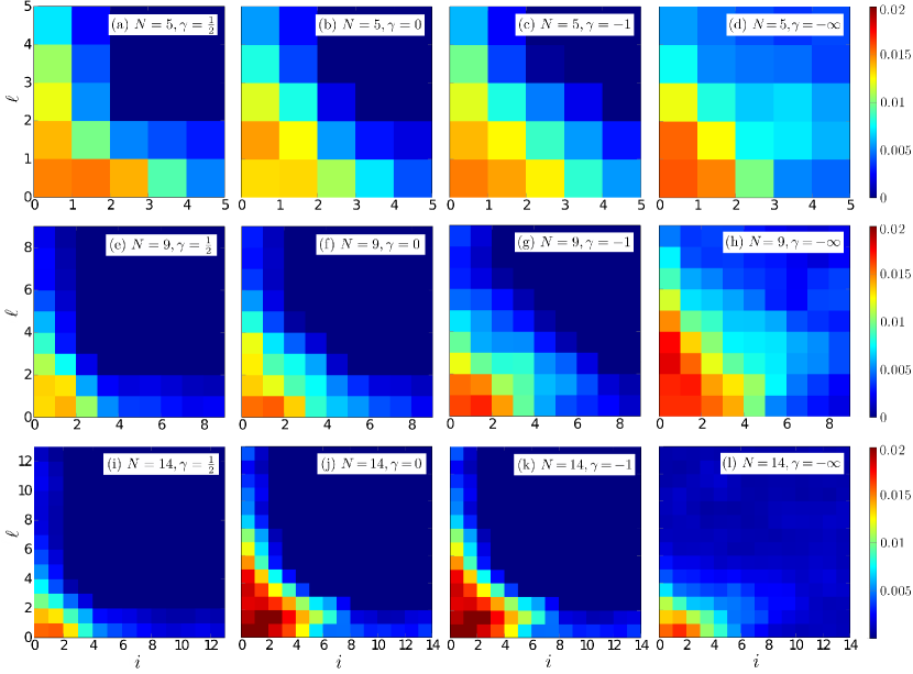
Figure 4: Saliency maps of the absolute value of derivatives of the relative $L^{2}$ loss w.r.t. $\{c_{i,\ell}\}$. Here, $N=5,9,1$ and $\gamma=-\infty,-1,0,\tfrac{1}{2}$ in Eq. (25). The loss function is always most sensitive to frequencies $c_{i,\ell}$ on the lower left of the saliency maps. Such a “resolution-invariance” indicates that having a larger $N$ but a moderate $\gamma>-\infty$ to include the frequencies in the lower-left part of this saliency map leads to a balance between efficiency and accuracy.

Appendix F Reconstructing learned dynamics

Table 10 shows that the errors from a new testing set, with randomly sampled time $t_{i}\sim\mathcal{U}(0,1.5)$, $i=1,\ldots,9$, do not differ significantly from the errors in the first row of Table 7. This suggests that our PDE learner can accurately extrapolate the solution to times beyond those of the training samples.

Table 10: Relative $L^{2}$ errors defined in Eq. (15) of trained models with different $\lambda$ on a new testing set of samples with noise-free coefficients ($\sigma=0$) and random sampling times $t_{j}\sim\mathcal{U}(0,1.5),j=1,\ldots,9$.

$\lambda$	$10^{-2}$	$10^{-1.75}$	$10^{-1.5}$	$10^{-1.25}$	$10^{-1}$	$10^{-0.75}$	$10^{-0.5}$
Mean relative $L^{2}$ error	$0.1977$	$0.0944$	$0.0229$	$0.0177$	$0.0158$	$0.0165$	$0.0156$
s.d. of relative $L^{2}$ error	$0.2590$	$0.1433$	$0.0039$	$0.0022$	$0.0013$	$0.0012$	$0.0006$

To make a comparison with the s-PINN method proposed in [15], we consider the following inverse-type problem of reconstructing the unknown potential $f(x,t)$ in

$$u_{t}=u_{xx}+f(x,t),$$ (28)

by approximating $f(x,t)\approx\hat{f}\coloneqq F[u;x,t,\Theta]-u_{xx}$. The function $u$ is taken to be

$$u(x,t)=\frac{\xi}{\sqrt{t+1}}\exp(-\tfrac{x^{2}}{4(t+1)})+\frac{\sin(x)}{\sqrt{t+1}}\exp(-\tfrac{x^{2}}{4(t+1)})$$ (29)

where $\xi\sim\mathcal{U}(\frac{1}{2},1)$ is i.i.d. sampled for different trajectories. Therefore, the true potential in Eq. (5) is

$$f(x,t)=\big{[}(t+1)\sin(x)+x\cos(x)\big{]}(t+1)^{(-3/2)}\exp(-\tfrac{x^{2}}{4(t+1)}),$$ (30)

which is independent of $u(x,t)$. We use 100 trajectories $u(x,t_{i})$ to learn the unknown potential with $t_{i}=i\Delta{t},\Delta{t}=0.1,i=0,...,10$. In the s-PINN method, since only $t$ is inputted, only one reconstructed $\hat{f}$ (which is the same for all trajectories) is outputted in the form of a spectral expansion. However, in our spectral neural DE learning method, $f(x,t)\approx\hat{f}=F[u;x,t,\Theta]-u_{xx}$ will be different for different inputted $u$ giving rise to a changing error along the time horizon. The mean and variance of the relative $L^{2}$ error $\frac{\|\hat{f}-f\|_{2}}{\|f\|_{2}}$ is plotted in Fig. 5.

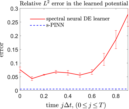
Figure 5: Comparison of the relative $L^{2}$ error in the potential in Eq. (5) learned from our proposed spectral neural DE learner and from the s-PINN method. Our spectral neural DE learner achieved an average relative $L^{2}$ error of $0.1$, while the s-PINN method, designed to input the exact form of the RHS of Eq. (5) with only one unknown potential, achieved better accuracy with an average relative $L^{2}$ error of about $0.01$.

When all but the potential on the RHS of Eq. (1) is known, the s-PINN is more preferable because more information is inputted as part of the loss function in [15]. Nevertheless, our spectral neural DE learner can still achieve a relative $L^{2}$ error $\sim 0.1$, indicating that without any prior information it can still reconstruct the unknown source term with acceptable accuracy. However, the accuracy of our spectral neural DE learner for reconstructing the potential $f$ deteriorates as the time horizon $t=j\Delta t$ increases. Since solutions at later times include errors from earlier times, minimizing Eq. (19) requires more accurate reconstruction of the dynamics (RHS of Eq. (1)) at earlier times than at later times.

References

- [1] L. Bar, N. Sochen, Unsupervised deep learning algorithm for PDE-based forward and inverse problems, arXiv preprint arXiv:1904.05417 (2019).
- [2] J.-T. Hsieh, S. Zhao, S. Eismann, L. Mirabella, S. Ermon, Learning neural PDE solvers with convergence guarantees, in: International Conference on Learning Representations, 2018.
- [3] L. Ruthotto, E. Haber, Deep neural networks motivated by partial differential equations, Journal of Mathematical Imaging and Vision 62 (3) (2020) 352–364.
- [4] J. Sirignano, J. F. MacArt, J. B. Freund, DPM: A deep learning PDE augmentation method with application to large-eddy simulation, Journal of Computational Physics 423 (2020) 109811.
- [5] J. Brandstetter, D. E. Worrall, M. Welling, Message passing neural PDE solvers, in: International Conference on Learning Representations, 2021.
- [6] M. Xia, S. Shao, T. Chou, Efficient scaling and moving techniques for spectral methods in unbounded domains, SIAM Journal on Scientific Computing 43 (5) (2021) A3244–A3268.
- [7] K. J. Burns, G. M. Vasil, J. S. Oishi, D. Lecoanet, B. P. Brown, Dedalus: A flexible framework for numerical simulations with spectral methods, Physical Review Research 2 (2) (2020) 023068.
- [8] J. Shen, T. Tang, Tao, L.-L. Wang, Spectral Methods: Algorithms, Analysis and Applications, Springer Science & Business Media, New York, 2011.
- [9] Z. Long, Y. Lu, X. Ma, B. Dong, PDE-net: Learning PDEs from data, in: International Conference on Machine Learning, PMLR, 2018, pp. 3208–3216.
- [10] Z. Long, Y. Lu, B. Dong, PDE-net 2.0: Learning PDEs from data with a numeric-symbolic hybrid deep network, Journal of Computational Physics 399 (2019) 108925.
- [11] H. Xu, H. Chang, D. Zhang, DL-PDE: Deep-learning based data-driven discovery of partial differential equations from discrete and noisy data, Communications in Computational Physics 29 (3) (2021) 698–728.
- [12] A. Anandkumar, K. Azizzadenesheli, K. Bhattacharya, N. Kovachki, Z. Li, B. Liu, A. Stuart, Neural operator: Graph kernel network for partial differential equations, in: ICLR 2020 Workshop on Integration of Deep Neural Models and Differential Equations, 2020.
- [13] Z. Li, N. B. Kovachki, K. Azizzadenesheli, K. Bhattacharya, A. Stuart, A. Anandkumar, et al., Fourier neural operator for parametric partial differential equations, in: International Conference on Learning Representations, 2020.
- [14] V. Fanaskov, I. Oseledets, Spectral neural operators, arXiv preprint arXiv:2205.10573 (2022).
- [15] M. Xia, L. Böttcher, T. Chou, Spectrally adapted physics-informed neural networks for solving unbounded domain problems, Machine Learning: Science and Technology 4 (2) (2023) 025024.
- [16] R. T. Chen, Y. Rubanova, J. Bettencourt, D. Duvenaud, Neural ordinary differential equations, in: Proceedings of the 32nd International Conference on Neural Information Processing Systems, 2018, pp. 6572–6583.
- [17] T. Tang, The Hermite spectral method for Gaussian-type functions, SIAM Journal on Scientific Computing 14 (3) (1993) 594–606.
- [18] M. Xia, S. Shao, T. Chou, A frequency-dependent p-adaptive technique for spectral methods, Journal of Computational Physics 446 (2021) 110627.
- [19] T. Chou, S. Shao, M. Xia, Adaptive Hermite spectral methods in unbounded domains, Applied Numerical Mathematics 183 (2023) 201–220.
- [20] J. Shen, L.-L. Wang, Sparse spectral approximations of high-dimensional problems based on hyperbolic cross, SIAM Journal on Numerical Analysis 48 (3) (2010) 1087–1109.
- [21] J. Shen, H. Yu, Efficient spectral sparse grid methods and applications to high-dimensional elliptic problems, SIAM Journal on Scientific Computing 32 (6) (2010) 3228–3250.
- [22] H. Bateman, Some recent researches on the motion of fluids, Monthly Weather Review 43 (4) (1915) 163–170.
- [23] X. Antoine, A. Arnold, C. Besse, M. Ehrhardt, A. Schädle, A review of transparent and artificial boundary conditions techniques for linear and nonlinear Schrödinger equations, Communications in Computational Physics 4 (4) (2008) 729–796.
- [24] K. He, X. Zhang, S. Ren, J. Sun, Deep residual learning for image recognition, in: Proceedings of the IEEE conference on computer vision and pattern recognition, 2016, pp. 770–778.
- [25] G. E. Hinton, N. Srivastava, A. Krizhevsky, I. Sutskever, R. R. Salakhutdinov, Improving neural networks by preventing co-adaptation of feature detectors, arXiv preprint arXiv:1207.0580 (2012).
- [26] N. Srivastava, G. E. Hinton, A. Krizhevsky, I. Sutskever, R. Salakhutdinov, Dropout: a simple way to prevent neural networks from overfitting, Journal of Machine Learning Research 15 (2014) 1929–1958.
- [27] Z. Chen, Y. Xiong, S. Shao, Numerical methods for the Wigner equation with unbounded potential, Journal of Scientific Computing 79 (1) (2019) 345–368.
- [28] S. Shao, T. Lu, W. Cai, Adaptive conservative cell average spectral element methods for transient Wigner equation in quantum transport, Communications in Computational Physics 9 (3) (2011) 711–739.
- [29] H.-J. Bungartz, M. Griebel, Sparse grids, Acta Numerica 13 (2004) 147–269.
- [30] C. Zenger, W. Hackbusch, Sparse grids, in: Proceedings of the Research Workshop of the Israel Science Foundation on Multiscale Phenomenon, Modelling and Computation, 1991, p. 86.
- [31] K. Simonyan, A. Vedaldi, A. Zisserman, Deep Inside Convolutional Networks: Visualising Image Classification Models and Saliency Maps, in: Proceedings of the International Conference on Learning Representation (ICLR), 2014, pp. 1–8.
- [32] B. Jin, W. Rundell, A tutorial on inverse problems for anomalous diffusion processes, Inverse problems 31 (3) (2015) 035003.