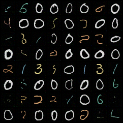
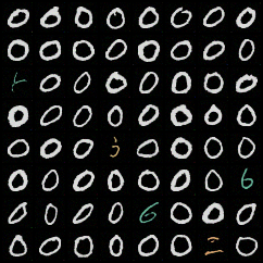
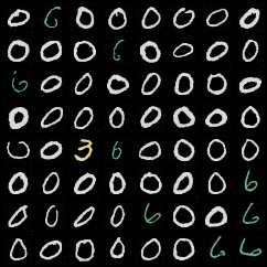
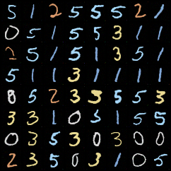
Compositional Sculpting of
Iterative Generative Processes

Timur Garipov
MIT CSAIL &Sebastiaan De Peuter
Aalto University &Ge Yang
MIT CSAIL
Institute for Artificial Intelligence
and Fundamental Interactions \ANDVikas Garg
Aalto University
YaiYai Ltd
&Samuel Kaski
Aalto University
University of Manchester &Tommi Jaakkola
MIT CSAIL
Correspondence to Timur Garipov (timur@csail.mit.edu).
Abstract

High training costs of generative models and the need to fine-tune them for specific tasks have created a strong interest in model reuse and composition. A key challenge in composing iterative generative processes, such as GFlowNets and diffusion models, is that to realize the desired target distribution, all steps of the generative process need to be coordinated, and satisfy delicate balance conditions. In this work, we propose Compositional Sculpting: a general approach for defining compositions of iterative generative processes. We then introduce a method for sampling from these compositions built on classifier guidance. We showcase ways to accomplish compositional sculpting in both GFlowNets and diffusion models. We highlight two binary operations — the harmonic mean (p1p2tensor-productsubscript𝑝1subscript𝑝2p_{1}\otimes p_{2}) and the contrast (p1\circlerighthalfblackp2subscript𝑝1\circlerighthalfblacksubscript𝑝2p_{1}{\,\circlerighthalfblack\,}p_{2}) between pairs, and the generalization of these operations to multiple component distributions. We offer empirical results on image and molecular generation tasks. Project codebase: https://github.com/timgaripov/compositional-sculpting.

1 Introduction

Large-scale general-purpose pre-training of machine learning models has produced impressive results in computer vision [1, 2, 3], image generation [4, 5, 6], natural language processing [7, 8, 9, 10, 11], robotics [12, 13, 14] and basic sciences [15]. By distilling vast amounts of data, such models can produce powerful inferences that lead to emergent capabilities beyond the specified training objective [16]. However, generic pre-trained models are often insufficient for specialized tasks in engineering and basic sciences. Field-adaptation via techniques such as explicit fine-tuning on bespoke datasets [17], human feedback [18], or cleverly designed prompts [19, 20] is therefore often required. An alternative approach is to compose the desired distribution using multiple simpler component models.

Compositional generation [21, 22, 23, 24, 25, 26, 27] views a complex target distribution in terms of simpler pre-trained building blocks which it can learn to mix and match into a tailored solution to a specialized task. Besides providing a way to combine and reuse previously trained models, composition is a powerful modeling approach. A composite model fuses knowledge from multiple sources: base models trained for different tasks, enabling increased capacity beyond that of any of the base models in isolation. If each individual base model captures a certain property of the data, composing such models provides a way to specify distributions over examples that exhibit multiple properties simultaneously [28]. The need to construct complex distributions adhering to multiple constraints arises in numerous practical multi-objective design problems such as multi-objective molecule generation [29, 30, 31]. In the context of multi-objective generation, compositional modeling provides mechanisms for adjustment and control of the resulting distribution, which enables exploration of different trade-offs between the objectives and constraints.

Prior work on generative model composition [21, 28, 23] has developed operations for piecing together Energy-Based Models (EBMs) via algebraic manipulations of their energy functions. For example, consider two distributions p1(x)exp{E1(x)}proportional-tosubscript𝑝1𝑥subscript𝐸1𝑥p_{1}(x)\varpropto\exp\{-E_{1}(x)\} and p2(x)exp{E2(x)}proportional-tosubscript𝑝2𝑥subscript𝐸2𝑥p_{2}(x)\varpropto\exp\{-E_{2}(x)\} induced by energy functions E1subscript𝐸1E_{1} and E2subscript𝐸2E_{2}. Their product pprod(x)p1(x)p2(x)exp((E1(x)+E2(x)))proportional-tosubscript𝑝prod𝑥subscript𝑝1𝑥subscript𝑝2𝑥proportional-tosubscript𝐸1𝑥subscript𝐸2𝑥p_{\text{prod}}(x)\varpropto p_{1}(x)p_{2}(x)\varpropto\exp\left(-\big{(}E_{1}(x)+E_{2}(x)\big{)}\right) and negation pneg(x)p1(x)/(p2(x))γexp((E1(x)γE2(x)))proportional-tosubscript𝑝neg𝑥subscript𝑝1𝑥superscriptsubscript𝑝2𝑥𝛾proportional-tosubscript𝐸1𝑥𝛾subscript𝐸2𝑥p_{\text{neg}}(x)\varpropto p_{1}(x)/(p_{2}(x))^{\gamma}\varpropto\exp\left(-\big{(}E_{1}(x)-\gamma E_{2}(x)\big{)}\right) correspond to operations on the underlying energy functions.

Iterative generative processes including diffusion models [32, 33, 5, 34] and GFlowNets [35, 36] progressively refine coarse objects into cleaner ones over multiple steps. The realization of effective compositions of these models is complicated by the fact that simple alterations in their generation processes result in non-trivial changes in the distributions of the final objects. For instance, the aforementioned product and negation between EBMs cannot be realized simply by means of adding or subtracting associated score-functions. Prior work addresses these challenges by connecting diffusion models with EBMs through annealed Markov-Chain Monte-Carlo (MCMC) inference. However, Metropolis-Hastings corrections are required to ensure that the annealing process reproduces the desired distribution [27].

Jain et al. [31] develop Multi-Objective GFlowNets (MOGFNs), an extension of GFlowNets for multi-objective optimization tasks. The goal of a vanilla GFlowNet model is to capture the distribution induced by a single reward (objective) function pθ(x)R(x)proportional-tosubscript𝑝𝜃𝑥𝑅𝑥p_{\theta}(x)\varpropto R(x) (see Section 2.1 for details of GFlowNet formulation). A Multi-Objective GFlowNet aims to learn a single conditional model that can realize distributions corresponding to various combinations (e.g. a convex combination) of multiple reward functions. While a single MOGFN effectively realizes a spectrum of compositions of base reward functions, the approach assumes access to the base rewards at training time. Moreover, MOFGNs require the set of possible composition operations to be specified at generative model training time. In this work, we address post hoc composition of pre-trained GFlowNets (or diffusion models) and provide a way to create compositions that need not be specified in advance.

In this work, we introduce Compositional Sculpting, a general approach for the composition of pre-trained models. We highlight two special examples of binary operations — harmonic mean: (p1p2tensor-productsubscript𝑝1subscript𝑝2p_{1}\otimes p_{2}) and contrast: (p1\circlerighthalfblackp2subscript𝑝1\circlerighthalfblacksubscript𝑝2p_{1}{\,\circlerighthalfblack\,}p_{2}). More general compositions are obtained as conditional distributions in a probabilistic model constructed on top of pre-trained base models. We show that these operations can be realized via classifier guidance. We provide results of empirical verification of our method on molecular generation (with GFlowNets) and image generation (with diffusion models).
Refer to caption
(a) p1subscript𝑝1p_{1}
Refer to caption
(b) p2subscript𝑝2p_{2}
Refer to caption
(c) p1p2tensor-productsubscript𝑝1subscript𝑝2p_{1}\otimes p_{2}
Refer to caption
(d) p1\circlerighthalfblackp2subscript𝑝1\circlerighthalfblacksubscript𝑝2p_{1}{\,\circlerighthalfblack\,}p_{2}
Refer to caption
(e) p1\circlelefthalfblackp2subscript𝑝1\circlelefthalfblacksubscript𝑝2p_{1}{\,\circlelefthalfblack\,}p_{2}
Refer to caption
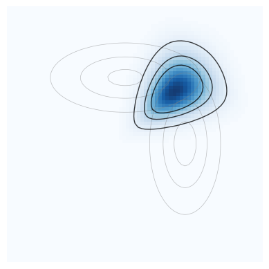
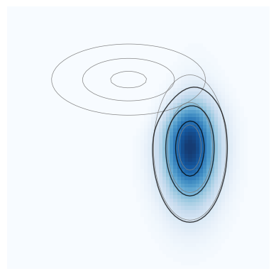
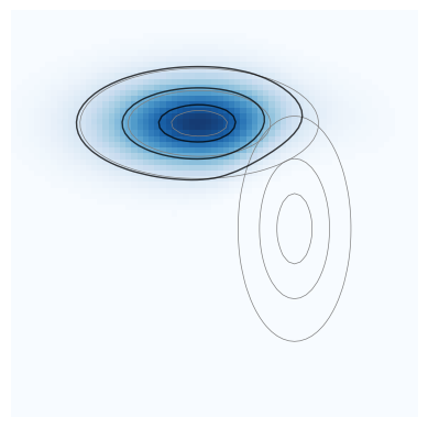
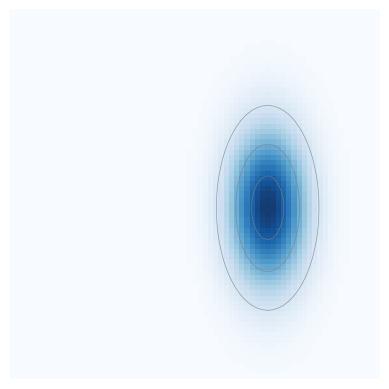
Figure 1: Composition operators. (a,b) base distributions p1subscript𝑝1p_{1} and p2subscript𝑝2p_{2}. (c) harmonic mean of p1subscript𝑝1p_{1} and p2subscript𝑝2p_{2}. (d) contrast of p1subscript𝑝1p_{1} with p2subscript𝑝2p_{2} (e) the reverse contrast p1\circlelefthalfblackp2subscript𝑝1\circlelefthalfblacksubscript𝑝2p_{1}{\,\circlelefthalfblack\,}p_{2}. Note \circlerighthalfblack\circlerighthalfblack{\,\circlerighthalfblack\,} is asymmetric. Grey lines show contours of PDF level sets of base Gaussian distributions p1subscript𝑝1p_{1}, p2subscript𝑝2p_{2}. Black lines show contours of PDF levels sets of composite distributions.

2 Background

2.1 Generative Flow Networks (GFlowNets)

GFlowNets [36, 35] are an approach for generating compositional objects (e.g. graphs). The objective of GFlowNet training is specified by a “reward function” R(x)0𝑅𝑥0R(x)\geq 0 defined on the set of objects 𝒳𝒳\mathcal{X}. The objective is to learn a generative model p(x)𝑝𝑥p(x) that assigns more probability mass on high-reward objects. Formally, GFlowNets seek to produce the distribution p(x)=R(x)/Z𝑝𝑥𝑅𝑥𝑍p(x)=\nicefrac{{R(x)}}{{Z}}, where Z=xR(x)𝑍subscript𝑥𝑅𝑥Z=\sum_{x}R(x).

Generative process.

The generation of a complete object x𝑥x is realized through a sequence of incremental changes of incomplete states s0s1sn1xsubscript𝑠0subscript𝑠1subscript𝑠𝑛1𝑥s_{0}\to s_{1}\to\ldots\to s_{n-1}\to x starting at the designated initial state s0subscript𝑠0s_{0}. Formally, the structure of possible generation trajectories τ=(s0s1sn1x)𝜏subscript𝑠0subscript𝑠1subscript𝑠𝑛1𝑥\tau=(s_{0}\to s_{1}\to\ldots\to s_{n-1}\to x) is captured by a DAG (𝒮,𝒜)𝒮𝒜(\mathcal{S},\mathcal{A}) where 𝒮𝒮\mathcal{S} is the set of states (both complete and incomplete) and 𝒜𝒜\mathcal{A} is the set of directed edges (actions) ss𝑠superscript𝑠s\to s^{\prime}. The set 𝒮𝒮\mathcal{S} has a designated initial state s0subscript𝑠0s_{0} and the set of complete objects (terminal states) 𝒳𝒳\mathcal{X} is a subset of 𝒮𝒮\mathcal{S}. Each generation trajectory τ𝜏\tau starts at the initial state s0subscript𝑠0s_{0}, follows the edges (ss)𝒜𝑠superscript𝑠𝒜(s\to s^{\prime})\in\mathcal{A} of the DAG, and terminates at one of the terminal states x𝒳𝑥𝒳x\in\mathcal{X}. We use |τ|𝜏|\tau| to denote the length of the trajectory (the number of transitions).

This sequential generation process is controlled by a parameterized stochastic “forward policy” PF(s|s;θ)subscript𝑃𝐹conditionalsuperscript𝑠𝑠𝜃P_{F}(s^{\prime}|s;\theta) which for each state s𝒮𝒳𝑠𝒮𝒳s\in\mathcal{S}\setminus\mathcal{X} specifies a probability distribution over all possible successor states s:(ss)𝒜:superscript𝑠𝑠superscript𝑠𝒜s^{\prime}\!:\!(s\to s^{\prime})\in\mathcal{A}. Generation is performed by starting at s0subscript𝑠0s_{0} and sequentially sampling transitions from the forward policy PF(|)P_{F}(\cdot|\cdot) until a terminal state is reached.

2.2 Diffusion Models

Diffusion models, see 32, 37, 33, 5, 34) are a family of generative models developed for continuous domains. Given a dataset of samples {x^i}i=1nsuperscriptsubscriptsubscript^𝑥𝑖𝑖1𝑛\{\hat{x}_{i}\}_{i=1}^{n} forming the empirical distribution p^(x)=1niδx^i(x)^𝑝𝑥1𝑛subscript𝑖subscript𝛿subscript^𝑥𝑖𝑥\hat{p}(x)=\frac{1}{n}\sum_{i}\delta_{\hat{x}_{i}}(x) in 𝒳=d𝒳superscript𝑑\mathcal{X}=\mathbb{R}^{d}, diffusion models seek to approximate p^(x)^𝑝𝑥\hat{p}(x) via a generative process p(x)𝑝𝑥p(x), which can then be used to generate new samples.

Stochastic Differential Equation (SDE) perspective.

We discuss diffusion models from the perspective of stochastic differential equations (SDE) [34]. A diffusion process is a noising process that gradually destroys the original “clean” data x𝑥x. It can be specified as a time-indexed collection of random variables {xt}t=0Tsuperscriptsubscriptsubscript𝑥𝑡𝑡0𝑇\{x_{t}\}_{t=0}^{T} in 𝒳=d𝒳superscript𝑑\mathcal{X}=\mathbb{R}^{d}. We use pt()subscript𝑝𝑡p_{t}(\cdot) to denote the density of the distribution of xtsubscript𝑥𝑡x_{t}. The process interpolates between the data distribution p0(x)=p^(x)subscript𝑝0𝑥^𝑝𝑥p_{0}(x)=\hat{p}(x) at t=0𝑡0t=0, and the prior distribution pT(x)subscript𝑝𝑇𝑥p_{T}(x) at t=T𝑡𝑇t=T, which is typically constructed to have a closed form (e.g. standard normal) to enable a simple sampling scheme. The evolution of xtsubscript𝑥𝑡x_{t} is described by the “forward SDE” dxt=ft(xt)dt+gtdwt𝑑subscript𝑥𝑡subscript𝑓𝑡subscript𝑥𝑡𝑑𝑡subscript𝑔𝑡𝑑subscript𝑤𝑡dx_{t}=f_{t}(x_{t})\,dt+g_{t}\,dw_{t}, where wtsubscript𝑤𝑡w_{t} is the standard Wiener process, the function ft:dd:subscript𝑓𝑡superscript𝑑superscript𝑑f_{t}:\mathbb{R}^{d}\to\mathbb{R}^{d} is called the drift coefficient and gtsubscript𝑔𝑡g_{t}\in\mathbb{R} is called the diffusion coefficient. Specific choices of ftsubscript𝑓𝑡f_{t} and gtsubscript𝑔𝑡g_{t} completely determine the process and give rise to the transition kernel pst(xt|xs)subscript𝑝𝑠𝑡conditionalsubscript𝑥𝑡subscript𝑥𝑠p_{st}(x_{t}|x_{s}) for 0s<tT0𝑠𝑡𝑇0\leq s<t\leq T (see [34] for examples).

Generative process.

Song et al. [34] invoke a result from the theory of stochastic processes [38] which gives the expression for the reverse-time process or “backward SDE”:

dxt=[ft(xt)gt2xlogpt(xt)]dt+gtdw¯t,𝑑subscript𝑥𝑡delimited-[]subscript𝑓𝑡subscript𝑥𝑡superscriptsubscript𝑔𝑡2subscript𝑥subscript𝑝𝑡subscript𝑥𝑡𝑑𝑡subscript𝑔𝑡𝑑subscript¯𝑤𝑡dx_{t}=\big{[}f_{t}(x_{t})-g_{t}^{2}\nabla_{x}\log p_{t}(x_{t})\big{]}\,dt+g_{t}\,d\overline{w}_{t}, (1)

where w¯tsubscript¯𝑤𝑡\overline{w}_{t} is the standard Wiener process in reversed time.

The backward SDE includes the known coefficients ftsubscript𝑓𝑡f_{t}, gtsubscript𝑔𝑡g_{t}, and the unknown score function xlogpt()subscript𝑥subscript𝑝𝑡\nabla_{x}\log p_{t}(\cdot) of the marginal distribution pt()subscript𝑝𝑡p_{t}(\cdot) at time t𝑡t. This score function is estimated by a deep neural network st(x;θ)xlogpt(x)subscript𝑠𝑡𝑥𝜃subscript𝑥subscript𝑝𝑡𝑥s_{t}(x;\theta)\approx\nabla_{x}\log p_{t}(x) (called “score-network”) with parameters θ𝜃\theta. Once the score-network st(;θ)subscript𝑠𝑡𝜃s_{t}(\cdot;\theta) is trained, samples can be generated via numerical integration of (1).

2.3 Classifier Guidance in Diffusion Models

Classifier guidance [32, 39] is a technique for controllable generation in diffusion models. Suppose that each example x0subscript𝑥0x_{0} is accompanied by a discrete class label y𝑦y. The goal is to sample from the conditional distribution p0(x0|y)subscript𝑝0conditionalsubscript𝑥0𝑦p_{0}(x_{0}|y). The Bayes rule pt(xt|y)pt(xt)pt(y|xt)proportional-tosubscript𝑝𝑡conditionalsubscript𝑥𝑡𝑦subscript𝑝𝑡subscript𝑥𝑡subscript𝑝𝑡conditional𝑦subscript𝑥𝑡p_{t}(x_{t}|y)\varpropto p_{t}(x_{t})p_{t}(y|x_{t}) implies the score-function decomposition xtlogpt(xt|y)=xtlogpt(xt)+xtlogpt(y|xt)subscriptsubscript𝑥𝑡subscript𝑝𝑡conditionalsubscript𝑥𝑡𝑦subscriptsubscript𝑥𝑡subscript𝑝𝑡subscript𝑥𝑡subscriptsubscript𝑥𝑡subscript𝑝𝑡conditional𝑦subscript𝑥𝑡\nabla_{x_{t}}\log p_{t}(x_{t}|y)=\nabla_{x_{t}}\log p_{t}(x_{t})+\nabla_{x_{t}}\log p_{t}(y|x_{t}), where the first term is already approximated by a pre-trained unconditional diffusion model and the second term can be derived from a time-dependent classifier pt(y|xt)subscript𝑝𝑡conditional𝑦subscript𝑥𝑡p_{t}(y|x_{t}). Therefore, the stated goal can be achieved by first training the classifier pt(y|xt)subscript𝑝𝑡conditional𝑦subscript𝑥𝑡p_{t}(y|x_{t}) using noisy samples xtsubscript𝑥𝑡x_{t} from the intermediate steps of the process, and then plugging in the expression for the conditional score into the sampling process (1).

2.4 “Energy” Operations

Prior work introduced energy operations, “product” and “negation”, for energy-based [21, 23] and diffusion [27] models. Given a pair of distributions p1(x)exp{E1(x)}proportional-tosubscript𝑝1𝑥subscript𝐸1𝑥p_{1}(x)\varpropto\exp\{-E_{1}(x)\}, p2(x)exp{E2(x)}proportional-tosubscript𝑝2𝑥subscript𝐸2𝑥p_{2}(x)\varpropto\exp\{-E_{2}(x)\} corresponding to the respective energy functions E1subscript𝐸1E_{1} and E2subscript𝐸2E_{2}, the “product” and “negation” operations are defined as

(p1prodp2)(x)exp{(E1(x)+E2(x))}p1(x)p2(x),proportional-tosubscript𝑝1prodsubscript𝑝2𝑥subscript𝐸1𝑥subscript𝐸2𝑥proportional-tosubscript𝑝1𝑥subscript𝑝2𝑥\displaystyle(p_{1}\,\text{prod}\;p_{2})(x)\varpropto\exp\Big{\{}\!-\!\Big{(}E_{1}(x)+E_{2}(x)\Big{)}\Big{\}}\varpropto p_{1}(x)p_{2}(x), (2)
(p1negγp2)(x)exp{(E1(x)γE2(x))}p1(x)(p2(x))γ.proportional-tosubscript𝑝1subscriptneg𝛾subscript𝑝2𝑥subscript𝐸1𝑥𝛾subscript𝐸2𝑥proportional-tosubscript𝑝1𝑥superscriptsubscript𝑝2𝑥𝛾\displaystyle(p_{1}\,\text{neg}_{\gamma}\;p_{2})(x)\varpropto\exp\Big{\{}\!-\!\Big{(}E_{1}(x)-\gamma E_{2}(x)\Big{)}\Big{\}}\varpropto\frac{p_{1}(x)}{\big{(}p_{2}(x)\big{)}^{\gamma}}. (3)

The product distribution (p1prodp2)(x)subscript𝑝1prodsubscript𝑝2𝑥(p_{1}\,\text{prod}\;p_{2})(x): (a) assigns relatively high likelihoods to points x𝑥x that have sufficiently high likelihoods under both base distributions at the same time; (b) assigns relatively low likelihoods to points x𝑥x that have close-to-zero likelihood under one (or both) p1subscript𝑝1p_{1}, p2subscript𝑝2p_{2}. The negation distribution (p1negγp2)(x)subscript𝑝1subscriptneg𝛾subscript𝑝2𝑥(p_{1}\,\text{neg}_{\gamma}\;p_{2})(x) (a) assigns relatively high likelihood to points x𝑥x that are likely under p1subscript𝑝1p_{1} but unlikely under p2subscript𝑝2p_{2}; (b) assigns relatively low likelihood to points x𝑥x that have low likelihood under p1subscript𝑝1p_{1} and high likelihood under p2subscript𝑝2p_{2}. The parameter γ>0𝛾0\gamma>0 controls the strength of negation. Informally, the product concentrates on points that are common in both p1subscript𝑝1p_{1} and p2subscript𝑝2p_{2}, and the negation concentrates on points that are common in p1subscript𝑝1p_{1} and uncommon in p2subscript𝑝2p_{2}. If p1subscript𝑝1p_{1} and p2subscript𝑝2p_{2} capture objects demonstrating two distinct concepts (e.g. p1subscript𝑝1p_{1}: images of circles; p2subscript𝑝2p_{2} images of green shapes), it is fair to say (again, informally) that the product and the negation resemble the logical operations of concept-intersection (“circle” AND “green”) and concept-negation (“circle” AND NOT “green”) respectively.

The “product” and “negation” can be realized in a natural way in energy-based models through simple algebraic operations on energy functions. However, realizing these operations on diffusion models is not as straightforward. The reason is that sampling in diffusion models requires the coordination of multiple steps of the denoising process. The simple addition of the time-dependent score functions does not result in a score function that represents the diffused product distribution111formally, xtlog(p0t(xt|x0)p1(x0)p2(x0)𝑑x0)xtlog(p0t(xt|x0)p1(x0)𝑑x0)+xtlog(p0t(xt|x0)p2(x0)𝑑x0)subscriptsubscript𝑥𝑡subscript𝑝0𝑡conditionalsubscript𝑥𝑡subscript𝑥0subscript𝑝1subscript𝑥0subscript𝑝2subscript𝑥0differential-dsubscript𝑥0subscript𝑥𝑡subscript𝑝0𝑡conditionalsubscript𝑥𝑡subscript𝑥0subscript𝑝1subscript𝑥0differential-dsubscript𝑥0subscript𝑥𝑡subscript𝑝0𝑡conditionalsubscript𝑥𝑡subscript𝑥0subscript𝑝2subscript𝑥0differential-dsubscript𝑥0\nabla_{x_{t}}\log\left(\int p_{0t}(x_{t}|x_{0})p_{1}(x_{0})p_{2}(x_{0})\,dx_{0}\right)\neq\nabla{x_{t}}\log\left(\int p_{0t}(x_{t}|x_{0})p_{1}(x_{0})\,dx_{0}\right)+\nabla{x_{t}}\log\left(\int p_{0t}(x_{t}|x_{0})p_{2}(x_{0})\,dx_{0}\right); we refer the reader to [27] for more details on the issue.. Du et al. [27] develop a method that corrects the sum-of-score-networks sampling via additional MCMC iterations nested under each step of the generation process.

3 Related Work

Generative model composition.

Hinton [28] developed a contrastive divergence minimization procedure for training products of tractable energy-based models. Learning mixtures of Generative Adversarial Networks has been addressed in [40], where the mixture components are learned simultaneously, and in [41], where the components are learned one by one in an adaptive boosting fashion. Grover and Ermon [42] developed algorithms for additive and multiplicative boosting of generative models. Following up on energy-based model operations [21, 28], Du et al. [23] studied the composition of deep energy-based models. Du et al. [27] developed algorithms for sampling from energy-based compositions (products, negations) of diffusion models, related to the focus of our work. The algorithm in [27] introduces additional MCMC sampling steps at each diffusion generation step to correct the originally biased sampling process (based on an algebraic combination of individual score functions) toward the target composition.

Our work proposes a new way to compose pre-trained diffusion models and introduces an unbiased sampling process based on classifier guidance to sample from the compositions. This avoids the need for corrective MCMC sampling required in prior work. Our work further applies to GFlowNets, and is, to the best of our knowledge, the first to address the composition of pre-trained GFlowNets.

This work focuses on the composition of pre-trained models. Assuming that each pre-trained model represents the distribution of examples demonstrating certain concepts (e.g. molecular properties), the composition of models is equivalent to concept composition (e.g. property “A” and property “B” satisfied simultaneously). The inverse problem is known as “unsupervised concept discovery”, where the goal is to automatically discover composable concepts from data. Unsupervised concept discovery and concept composition methods have been proposed for energy-based models [24] and for text-to-image diffusion models [43].

Controllable generation.

Generative model composition is a form of post-training control of the generation process, an established area of research in generative modeling. A simple approach to control is conditional generation, which can be achieved by training a conditional generative model pθ(x|c)subscript𝑝𝜃conditional𝑥𝑐p_{\theta}(x|c) on pairs (x,c)𝑥𝑐(x,c) of objects x𝑥x and conditioning information c𝑐c. Types of conditioning information can include class labels [39] or more structured data such as text prompts [6, 4, 44], semantic maps, and other images for image-to-image translation [4]. This approach assumes that the generation control operations are specified at training time and the training data is annotated with conditioning attributes. Classifier guidance [32] provides a way to generate samples from conditional distributions that need not be specified at training time. The guidance is realized by a classifier that is trained on examples xtsubscript𝑥𝑡x_{t} (both clean and noisy) accompanied by conditioning labels c𝑐c. Dhariwal and Nichol [39] apply classifier guidance on top of unconditional or conditional diffusion models to improve the fidelity of generated images. Ho and Salimans [45] develop classifier-free guidance where the conditional and unconditional score functions are trained simultaneously and combined at inference time to guide the generation. In ControlNet [17], an additional network is trained to enable a pre-trained diffusion model to incorporate additional, previously unavailable, conditioning information. Meng et al. [46] and Couairon et al. [47] develop semantic image editing methods based on applying noise to the original image and then running the reverse denoising process to generate an edited image, possibly conditioned on a segmentation mask [47].

Similar to conditional diffusion models, conditional GFlowNets have been used to condition generation on reward exponents [36] or combinations of multiple predefined reward functions [31].

Note that the methods developed in this work can be combined with conditional generative models, for example, conditional diffusion models (or GFlowNets) p(x|c1),,p(x|cm)𝑝conditional𝑥subscript𝑐1𝑝conditional𝑥subscript𝑐𝑚p(x|c_{1}),\ldots,p(x|c_{m}) can act as base generative models to be composed.

Compositional generalization.

The notion of compositionality has a broad spectrum of interpretations across a variety of disciplines including linguistics, cognitive science, and philosophy. Hupkes et al. [48] collect a list of aspects of compositionality from linguistical and philosophical theories and designs practical tests for neural language models covering all aspects. Conwell and Ullman [49] empirically examine the relational understanding of DALL-E 2 [50], a text-guided image generation model, and point out limitations in the model’s ability to capture relations such as “in”, “on”, “hanging over”, etc. In this work, we focus on a narrow but well-defined type of composition where we seek to algebraically combine (compose) probability densities in a controllable fashion, such that we can emphasize or de-emphasize regions in the data space where specific base distributions have high density. Our methods are developed for the setting where we are given access to GFlowNets or diffusion models which can generate samples from the probability distributions we wish to compose.

Connections between GFlowNets and diffusion models.

We develop composition operations and methods for sampling from composite distributions for both GFlowNets and diffusion models. The fact that similar methods apply to both is rooted in deep connections between the two modeling frameworks. GFlowNets were initially developed for generating discrete (structured) data [36] and diffusion models were initially developed for continuous data [32, 5]. Lahlou et al. [51] develop an extension of GFlowNets for DAGs with continuous state-action spaces. Zhang et al. [52] point out unifying connections between GFlowNets and other generative model families, including diffusion models. Diffusion models in a fixed-time discretization can be interpreted as continuous GFlowNets of a certain structure. Zhang et al. [52] notice that the discrete DAG flow-matching condition, central to mathematical foundations of GFlowNets [35], is analogous to the Fokker-Planck equation (Kolmogorov forward equation), underlying mathematical analysis of continuous-time diffusion models [34]. In this work, we articulate another aspect of the relation between GFlowNets and diffusion models: in Section 5.1 we derive the expressions for mixture GFlowNet policies and classifier-guided GFlowNet policies analogous to those derived for diffusion models in prior work [53, 54, 32, 39].

4 Compositional Sculpting of Generative Models

Consider a scenario where we can access a number of pre-trained generative models. Each of these “base models” gives rise to a generative distribution pi(x)subscript𝑝𝑖𝑥p_{i}(x) over a common domain 𝒳𝒳\mathcal{X}. We may wish to compose these distributions such that we can, say, draw samples that are likely to arise from p1(x)subscript𝑝1𝑥p_{1}(x) and p2(x)subscript𝑝2𝑥p_{2}(x), or that are likely to arise from p1(x)subscript𝑝1𝑥p_{1}(x) but not from p2(x)subscript𝑝2𝑥p_{2}(x). In other words, we wish to specify a composition whose generative distribution we can shape to emphasize and de-emphasize specific base models.

4.1 Binary Composition Operations

For the moment, let us focus on controllably composing two base models. One option is to specify the composition as a weighted combination p~(x)=i=12ωipi(x)~𝑝𝑥superscriptsubscript𝑖12subscript𝜔𝑖subscript𝑝𝑖𝑥\widetilde{p}(x)=\sum_{i=1}^{2}\omega_{i}p_{i}(x) with positive weights ω1,ω2subscript𝜔1subscript𝜔2\omega_{1},\omega_{2} which sum to one. These weights allow us to set the prevalence of each base model in the composition. However, beyond that our control over the composition is limited. We cannot emphasize regions where, say, p1subscript𝑝1p_{1} and p2subscript𝑝2p_{2} both have high density, or de-emphasize regions where p2subscript𝑝2p_{2} has high density.

A much more flexible method for shaping a prior distribution p~(x)~𝑝𝑥\widetilde{p}(x) to our desires is conditioning. Following Bayesian inference methodology, we know that when we condition x𝑥x on some observation y𝑦y, the resulting posterior takes the form p~(x|y)p~(y|x)p~(x)proportional-to~𝑝conditional𝑥𝑦~𝑝conditional𝑦𝑥~𝑝𝑥\widetilde{p}(x|y)\propto\widetilde{p}(y|x)\widetilde{p}(x). Points x𝑥x that match observation y𝑦y according to p~(y|x)~𝑝conditional𝑦𝑥\widetilde{p}(y|x) will have increased density, whereas the density of points that do not match it decreases. Intuitively, the term p~(y|x)~𝑝conditional𝑦𝑥\widetilde{p}(y|x) has shaped the prior p~(x)~𝑝𝑥\widetilde{p}(x) according to y𝑦y.

If we define the observation y1{1,2}subscript𝑦112y_{1}\in\{1,2\} as the event that x𝑥x was generated by a specific base model, we can shape the prior based on the densities of the base models. We start by defining a uniform prior over yksubscript𝑦𝑘y_{k}, and by defining the conditional density p(x|y1=i)𝑝conditional𝑥subscript𝑦1𝑖p(x|y_{1}=i) to represent the fact that x𝑥x was generated from pi(x)subscript𝑝𝑖𝑥p_{i}(x). This gives us the following model:

p~(x|y1=1)=p1(x),p~(x|y1=2)=p2(x),p~(y1=1)=p~(y1=2)=12,p~(x)=i=12p~(x|y1=i)p~(y1=i),formulae-sequenceformulae-sequence~𝑝conditional𝑥subscript𝑦11subscript𝑝1𝑥formulae-sequence~𝑝conditional𝑥subscript𝑦12subscript𝑝2𝑥~𝑝subscript𝑦11~𝑝subscript𝑦1212~𝑝𝑥superscriptsubscript𝑖12~𝑝conditional𝑥subscript𝑦1𝑖~𝑝subscript𝑦1𝑖\widetilde{p}(x|y_{1}\!=\!1)=p_{1}(x),\quad\widetilde{p}(x|y_{1}\!=\!2)=p_{2}(x),\quad\widetilde{p}(y_{1}\!=\!1)=\widetilde{p}(y_{1}\!=\!2)=\frac{1}{2},\quad\widetilde{p}(x)=\sum_{i=1}^{2}\widetilde{p}(x|y_{1}\!=\!i)\widetilde{p}(y_{1}\!=\!i), (4)

Notice that under this model, the prior p~(x)~𝑝𝑥\widetilde{p}(x) is simply a uniform mixture of the base models. The posterior probability p~(y1=1|x)~𝑝subscript𝑦1conditional1𝑥\widetilde{p}(y_{1}\!=\!1|x) implied by this model tells us how likely it is that x𝑥x was generated by p1(x)subscript𝑝1𝑥p_{1}(x) rather than p2(x)subscript𝑝2𝑥p_{2}(x):

p~(y1=1|x)=1p~(y1=2|x)=p1(x)p1(x)+p2(x),~𝑝subscript𝑦1conditional1𝑥1~𝑝subscript𝑦1conditional2𝑥subscript𝑝1𝑥subscript𝑝1𝑥subscript𝑝2𝑥\widetilde{p}(y_{1}\!=\!1|x)=1-\widetilde{p}(y_{1}\!=\!2|x)=\frac{p_{1}(x)}{p_{1}(x)+p_{2}(x)}, (5)

Note that p~(y1=1|x)~𝑝subscript𝑦1conditional1𝑥\widetilde{p}(y_{1}\!=\!1|x) is the output of the optimal classifier trained to tell apart distributions p1(x)subscript𝑝1𝑥p_{1}(x) and p2(x)subscript𝑝2𝑥p_{2}(x).

The goal stated at the beginning of this section was to realize compositions which would generate samples likely to arise from both p1(x)subscript𝑝1𝑥p_{1}(x) and p2(x)subscript𝑝2𝑥p_{2}(x) or likely to arise from p1(x)subscript𝑝1𝑥p_{1}(x) but not p2(x)subscript𝑝2𝑥p_{2}(x). To this end we introduce a second observation y2{1,2}subscript𝑦212y_{2}\in\{1,2\} such that y1subscript𝑦1y_{1} and y2subscript𝑦2y_{2} are independent and identically distributed given x𝑥x. The resulting full model and inferred posterior are:

p~(x,y1,y2)=p~(x)p~(y1|x)p~(y2|x),p~(x)=12p1(x)+12p2(x),p~(yk=i|x)=pi(x)p1(x)+p2(x),k,i{1,2},formulae-sequence~𝑝𝑥subscript𝑦1subscript𝑦2~𝑝𝑥~𝑝conditionalsubscript𝑦1𝑥~𝑝conditionalsubscript𝑦2𝑥formulae-sequence~𝑝𝑥12subscript𝑝1𝑥12subscript𝑝2𝑥formulae-sequence~𝑝subscript𝑦𝑘conditional𝑖𝑥subscript𝑝𝑖𝑥subscript𝑝1𝑥subscript𝑝2𝑥𝑘𝑖12\widetilde{p}(x,y_{1},y_{2})=\widetilde{p}(x)\widetilde{p}(y_{1}|x)\widetilde{p}(y_{2}|x),\quad\widetilde{p}(x)=\frac{1}{2}p_{1}(x)+\frac{1}{2}p_{2}(x),\quad\widetilde{p}(y_{k}\!=\!i|x)=\frac{p_{i}(x)}{p_{1}(x)+p_{2}(x)},\;k,i\in\{1,2\}, (6)
p~(x|y1=i,y2=j)p~(x)p~(y1=i|x)p~(y2=j|x)pi(x)pj(x)p1(x)+p2(x).proportional-to~𝑝formulae-sequenceconditional𝑥subscript𝑦1𝑖subscript𝑦2𝑗~𝑝𝑥~𝑝subscript𝑦1conditional𝑖𝑥~𝑝subscript𝑦2conditional𝑗𝑥proportional-tosubscript𝑝𝑖𝑥subscript𝑝𝑗𝑥subscript𝑝1𝑥subscript𝑝2𝑥\widetilde{p}(x|y_{1}\!=\!i,y_{2}\!=\!j)\varpropto\widetilde{p}(x)\widetilde{p}(y_{1}\!=\!i|x)\widetilde{p}(y_{2}\!=\!j|x)\varpropto\frac{p_{i}(x)p_{j}(x)}{p_{1}(x)+p_{2}(x)}. (7)

The posterior p~(x|y1=i,y2=j)~𝑝formulae-sequenceconditional𝑥subscript𝑦1𝑖subscript𝑦2𝑗\widetilde{p}(x|y_{1}\!=\!i,y_{2}\!=\!j) shows clearly how conditioning on the observations y1,y2subscript𝑦1subscript𝑦2y_{1},y_{2} has shaped the prior mixture into a new expression which accentuates regions in the posterior where the observed base models i,j𝑖𝑗i,j have high density.

Conditioning on observations y1=1subscript𝑦11y_{1}\!=\!1 (“x𝑥x is likely to have been drawn from p1subscript𝑝1p_{1} rather than p2subscript𝑝2p_{2}”) and y2=2subscript𝑦22y_{2}\!=\!2 (“x𝑥x is likely to have been drawn from p2subscript𝑝2p_{2} rather than p1subscript𝑝1p_{1}”), or equivalently y1=2,y2=1formulae-sequencesubscript𝑦12subscript𝑦21y_{1}\!=\!2,y_{2}\!=\!1, results in the posterior distribution

(p1p2)(x):=p(x|y1=1,y2=2)p1(x)p2(x)p1(x)+p2(x).assigntensor-productsubscript𝑝1subscript𝑝2𝑥𝑝formulae-sequenceconditional𝑥subscript𝑦11subscript𝑦22proportional-tosubscript𝑝1𝑥subscript𝑝2𝑥subscript𝑝1𝑥subscript𝑝2𝑥(p_{1}\otimes p_{2})(x):=p(x|y_{1}\!=\!1,y_{2}\!=\!2)\varpropto\frac{p_{1}(x)p_{2}(x)}{p_{1}(x)+p_{2}(x)}. (8)

We will refer to this posterior as the “harmonic mean of p1subscript𝑝1p_{1} and p2subscript𝑝2p_{2}”, and denote it as a binary operation p1p2tensor-productsubscript𝑝1subscript𝑝2p_{1}\otimes p_{2}. Its value is high only at points that have high likelihood under both p1(x)subscript𝑝1𝑥p_{1}(x) and p2(x)subscript𝑝2𝑥p_{2}(x) at the same time (Figure 1(c)). Thus, the harmonic mean is an alternative to the product operation for EBMs. The harmonic mean is commutative (p1p2=p2p1tensor-productsubscript𝑝1subscript𝑝2tensor-productsubscript𝑝2subscript𝑝1p_{1}\otimes p_{2}=p_{2}\otimes p_{1}) and is undefined when p1subscript𝑝1p_{1} and p2subscript𝑝2p_{2} have disjoint supports, since then the RHS of (8) is zero everywhere.

Conditioning on observations y1=1subscript𝑦11y_{1}\!=\!1 (“x𝑥x is likely to have been drawn from p1subscript𝑝1p_{1} rather than p2subscript𝑝2p_{2}”) and y2=1subscript𝑦21y_{2}\!=\!1 (same) results in the posterior distribution

(p1\circlerighthalfblackp2)(x):=p~(x|y1=1,y2=1)(p1(x))2p1(x)+p2(x).assignsubscript𝑝1\circlerighthalfblacksubscript𝑝2𝑥~𝑝formulae-sequenceconditional𝑥subscript𝑦11subscript𝑦21proportional-tosuperscriptsubscript𝑝1𝑥2subscript𝑝1𝑥subscript𝑝2𝑥(p_{1}{\,\circlerighthalfblack\,}p_{2})(x):=\widetilde{p}(x|y_{1}\!=\!1,y_{2}\!=\!1)\varpropto\frac{\big{(}p_{1}(x)\big{)}^{2}}{p_{1}(x)+p_{2}(x)}. (9)

We refer to this operation, providing an alternative to the negation operation in EBMs, as the “contrast of p1subscript𝑝1p_{1} and p2subscript𝑝2p_{2}”, and will denote it as a binary operator (p1\circlerighthalfblackp2)(x)subscript𝑝1\circlerighthalfblacksubscript𝑝2𝑥(p_{1}{\,\circlerighthalfblack\,}p_{2})(x). The ratio in equation (9) is strictly increasing as a function of p1(x)subscript𝑝1𝑥p_{1}(x) and strictly decreasing as a function of p2(x)subscript𝑝2𝑥p_{2}(x), so that the ratio is high when p1(x)subscript𝑝1𝑥p_{1}(x) is high and p2(x)subscript𝑝2𝑥p_{2}(x) is low (Figure 1(d)). The contrast is not commutative (p1\circlerighthalfblackp2p2\circlerighthalfblackp1subscript𝑝1\circlerighthalfblacksubscript𝑝2subscript𝑝2\circlerighthalfblacksubscript𝑝1p_{1}{\,\circlerighthalfblack\,}p_{2}\neq p_{2}{\,\circlerighthalfblack\,}p_{1}, unless p1=p2subscript𝑝1subscript𝑝2p_{1}=p_{2}). We will denote the reverse contrast as p1\circlelefthalfblackp2=p2\circlerighthalfblackp1subscript𝑝1\circlelefthalfblacksubscript𝑝2subscript𝑝2\circlerighthalfblacksubscript𝑝1p_{1}{\,\circlelefthalfblack\,}p_{2}=p_{2}{\,\circlerighthalfblack\,}p_{1}.

Note that the original distributions p1subscript𝑝1p_{1} and p2subscript𝑝2p_{2} can be expressed as mixtures of the harmonic mean and the contrast distributions:

p1=Z(p1p2)+Z\circlerighthalfblack(p1\circlerighthalfblackp2),p2=Z(p1p2)+Z\circlerighthalfblack(p2\circlerighthalfblackp1),Z=xp1(x)p2(x)p1(x)+p2(x)=1Z\circlerighthalfblack.formulae-sequencesubscript𝑝1subscript𝑍tensor-producttensor-productsubscript𝑝1subscript𝑝2subscript𝑍\circlerighthalfblacksubscript𝑝1\circlerighthalfblacksubscript𝑝2formulae-sequencesubscript𝑝2subscript𝑍tensor-producttensor-productsubscript𝑝1subscript𝑝2subscript𝑍\circlerighthalfblacksubscript𝑝2\circlerighthalfblacksubscript𝑝1subscript𝑍tensor-productsubscript𝑥subscript𝑝1𝑥subscript𝑝2𝑥subscript𝑝1𝑥subscript𝑝2𝑥1subscript𝑍\circlerighthalfblack\displaystyle p_{1}=Z_{\otimes}(p_{1}\otimes p_{2})+Z_{\,\circlerighthalfblack\,}(p_{1}{\,\circlerighthalfblack\,}p_{2}),\quad p_{2}=Z_{\otimes}(p_{1}\otimes p_{2})+Z_{\,\circlerighthalfblack\,}(p_{2}{\,\circlerighthalfblack\,}p_{1}),\quad Z_{\otimes}=\sum_{x}\frac{p_{1}(x)p_{2}(x)}{p_{1}(x)+p_{2}(x)}=1-Z_{\,\circlerighthalfblack\,}.

Controlling the individual contributions of p1subscript𝑝1p_{1} and p2subscript𝑝2p_{2} to the composition.

We modify model (6) and introduce an interpolation parameter α𝛼\alpha in order to have more control over the extent of individual contributions of p1subscript𝑝1p_{1} and p2subscript𝑝2p_{2} to the composition:

p~(x,y1,y2;α)=p~(x)p~(y1|x)p~(y2|x;α),p~(x)=12p1(x)+12p2(x),formulae-sequence~𝑝𝑥subscript𝑦1subscript𝑦2𝛼~𝑝𝑥~𝑝conditionalsubscript𝑦1𝑥~𝑝conditionalsubscript𝑦2𝑥𝛼~𝑝𝑥12subscript𝑝1𝑥12subscript𝑝2𝑥\displaystyle\widetilde{p}(x,y_{1},y_{2};\alpha)=\widetilde{p}(x)\widetilde{p}(y_{1}|x)\widetilde{p}(y_{2}|x;\alpha),~{}~{}\widetilde{p}(x)=\frac{1}{2}p_{1}(x)+\frac{1}{2}p_{2}(x), (10a)
p~(y1=i|x)=pi(x)p1(x)+p2(x),p~(y2=i|x;α)=(αp1(x))[i=1]((1α)p2(x))[i=2]αp1(x)+(1α)p2(x),formulae-sequence~𝑝subscript𝑦1conditional𝑖𝑥subscript𝑝𝑖𝑥subscript𝑝1𝑥subscript𝑝2𝑥~𝑝subscript𝑦2conditional𝑖𝑥𝛼superscript𝛼subscript𝑝1𝑥delimited-[]𝑖1superscript1𝛼subscript𝑝2𝑥delimited-[]𝑖2𝛼subscript𝑝1𝑥1𝛼subscript𝑝2𝑥\displaystyle\widetilde{p}(y_{1}\!=\!i|x)=\frac{p_{i}(x)}{p_{1}(x)+p_{2}(x)},~{}~{}\widetilde{p}(y_{2}\!=\!i|x;\alpha)\!=\!\frac{\big{(}\alpha p_{1}(x)\big{)}^{[i=1]}\cdot\big{(}(1\!-\!\alpha)p_{2}(x)\big{)}^{[i=2]}}{\alpha p_{1}(x)+(1-\alpha)p_{2}(x)}, (10b)

where α(0,1)𝛼01\alpha\in(0,1) and []delimited-[][\cdot] denotes the indicator function. Conditional distributions in this model give harmonic interpolation222the harmonic interpolation approaches p1subscript𝑝1p_{1} when α0𝛼0\alpha\to 0 and p2subscript𝑝2p_{2} when α1𝛼1\alpha\to 1 and parameterized contrast:

(p1(1α)p2)(x)p1(x)p2(x)αp1(x)+(1α)p2(x),(p1\circlerighthalfblack(1α)p2)(x)(p1(x))2αp1(x)+(1α)p2(x).formulae-sequenceproportional-tosubscripttensor-product1𝛼subscript𝑝1subscript𝑝2𝑥subscript𝑝1𝑥subscript𝑝2𝑥𝛼subscript𝑝1𝑥1𝛼subscript𝑝2𝑥proportional-tosubscript𝑝1subscript\circlerighthalfblack1𝛼subscript𝑝2𝑥superscriptsubscript𝑝1𝑥2𝛼subscript𝑝1𝑥1𝛼subscript𝑝2𝑥(p_{1}\otimes_{(1-\alpha)}p_{2})(x)\varpropto\frac{p_{1}(x)p_{2}(x)}{\alpha p_{1}(x)+(1-\alpha)p_{2}(x)},\quad(p_{1}{\,\circlerighthalfblack\,}_{(1-\alpha)}\ p_{2})(x)\varpropto\frac{\big{(}p_{1}(x)\big{)}^{2}}{\alpha p_{1}(x)+(1-\alpha)p_{2}(x)}. (11)
Refer to caption
(a) Base distributions p1subscript𝑝1p_{1}, p2subscript𝑝2p_{2}
Refer to caption
(b) HM (ours), Product
Refer to caption
(c) Contrasts p1\circlerighthalfblack(1α)p2subscript𝑝1subscript\circlerighthalfblack1𝛼subscript𝑝2p_{1}{\,\circlerighthalfblack\,}_{(1-\alpha)}\;p_{2} (ours)
Refer to caption
(d) Negations p1negγp2subscript𝑝1subscriptneg𝛾subscript𝑝2p_{1}\,\text{neg}_{\gamma}\;p_{2}
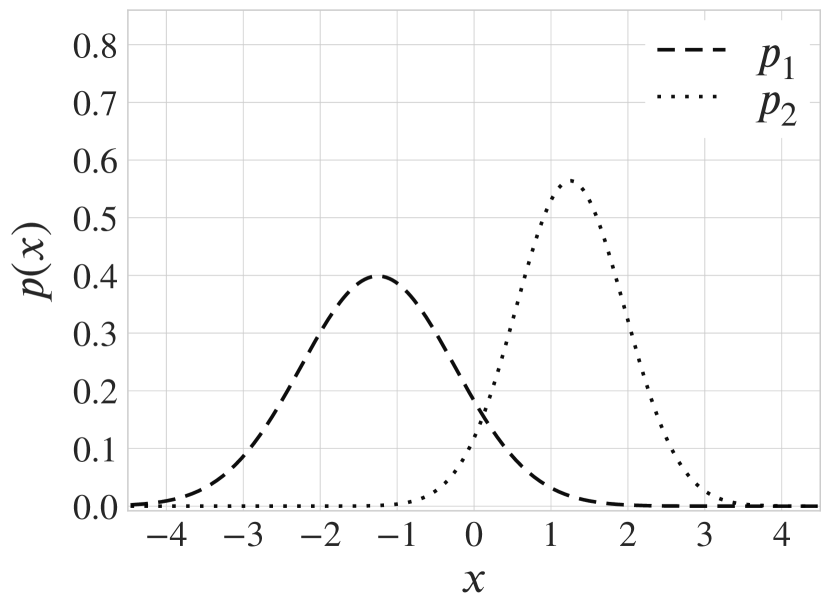
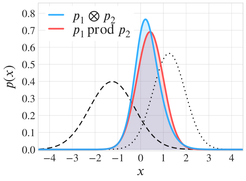
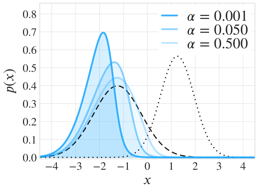
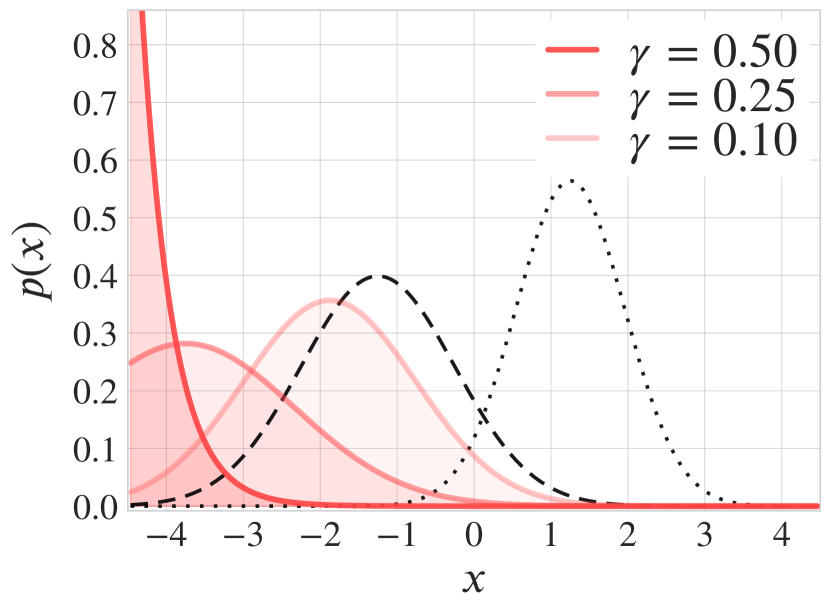
Figure 2: Compositional sculpting and energy operations applied to 1D Gaussian distributions. (a) Densities of base 1D Gaussian distributions p1(x)=𝒩(x;5/4,1)subscript𝑝1𝑥𝒩𝑥541p_{1}(x)=\mathcal{N}(x;-\nicefrac{{5}}{{4}},1), p2(x)=𝒩(x;5/4,1/2)subscript𝑝2𝑥𝒩𝑥5412p_{2}(x)=\mathcal{N}(x;\nicefrac{{5}}{{4}},\nicefrac{{1}}{{2}}). (b) harmonic mean p1p2tensor-productsubscript𝑝1subscript𝑝2p_{1}\otimes p_{2} and product p1prodp2subscript𝑝1prodsubscript𝑝2p_{1}\,\text{prod}\;p_{2} (c) parameterized contrasts p1\circlerighthalfblack(1α)p2subscript𝑝1subscript\circlerighthalfblack1𝛼subscript𝑝2p_{1}{\,\circlerighthalfblack\,}_{\!(1-\alpha)}\;p_{2} at different values of α𝛼\alpha (d) negations p1negγp2subscript𝑝1subscriptneg𝛾subscript𝑝2p_{1}\,\text{neg}_{\gamma}\;p_{2} at different values of γ𝛾\gamma. The curves show the probability density functions of base distributions and their compositions.

Comparison with “energy” operations.

The harmonic mean and contrast operations we have introduced here are anologous to the product and negation operations for EBMs respectively. Although the harmonic mean and product operations are quite similar in practice, unlike the negation operation our proposed contrast operation always results in a valid probability distribution. Figure 2 shows the results of these operations applied to two Gaussian distributions. The harmonic mean and product, shown in panel 2(b), are both concentrated on points that have high probability under both Gaussians. Figure 2(c) shows parameterized contrasts p1\circlerighthalfblack(1α)p2subscript𝑝1subscript\circlerighthalfblack1𝛼subscript𝑝2p_{1}{\,\circlerighthalfblack\,}_{(1-\alpha)}p_{2} at different values of α𝛼\alpha, and panel 2(d) shows negations p1negγp2subscript𝑝1subscriptneg𝛾subscript𝑝2p_{1}\,\text{neg}_{\gamma}\;p_{2} at different values of γ𝛾\gamma. The effect of negation at γ=0.1𝛾0.1\gamma=0.1 resembles the effect of the contrast operation: the density retreats from the high likelihood region of p2subscript𝑝2p_{2}. However, as γ𝛾\gamma increases to 0.50.50.5 the distribution starts to concentrate excessively on the values x<3𝑥3x<-3. This is due to the instability of division p1(x)/(p2(x))γsubscript𝑝1𝑥superscriptsubscript𝑝2𝑥𝛾\nicefrac{{p_{1}(x)}}{{(p_{2}(x))^{\gamma}}} in regions where p2(x)0subscript𝑝2𝑥0p_{2}(x)\to 0. Proposition B.1 in Appendix B shows that the negation p1negγp2subscript𝑝1subscriptneg𝛾subscript𝑝2p_{1}\,\text{neg}_{\gamma}\;p_{2} in many cases results in an improper (non-normalizable) distribution.

Operation chaining.

As the binary operations we have introduced result in proper distributions, we can create new N𝑁N-ary operations by chaining binary (and N𝑁N-ary) operations together. For instance, chaining binary harmonic means gives the harmonic mean of three distributions

((p1p2)p3)(x)=(p1(p2p3))(x)p1(x)p2(x)p3(x)p1(x)p2(x)+p1(x)p3(x)+p2(x)p3(x).tensor-producttensor-productsubscript𝑝1subscript𝑝2subscript𝑝3𝑥tensor-productsubscript𝑝1tensor-productsubscript𝑝2subscript𝑝3𝑥proportional-tosubscript𝑝1𝑥subscript𝑝2𝑥subscript𝑝3𝑥subscript𝑝1𝑥subscript𝑝2𝑥subscript𝑝1𝑥subscript𝑝3𝑥subscript𝑝2𝑥subscript𝑝3𝑥((p_{1}\otimes p_{2})\otimes p_{3})(x)=(p_{1}\otimes(p_{2}\otimes p_{3}))(x)\varpropto\frac{p_{1}(x)p_{2}(x)p_{3}(x)}{p_{1}(x)p_{2}(x)+p_{1}(x)p_{3}(x)+p_{2}(x)p_{3}(x)}. (12)

4.2 Compositional Sculpting: General Approach

The approach we used above for specifying compositions of two base models controlled by two observations can be generalized to compositions of m𝑚m base models p1(x),,pm(x)subscript𝑝1𝑥subscript𝑝𝑚𝑥p_{1}(x),\dots,p_{m}(x) controlled by n𝑛n observations. At the end of the previous section we showed that operator chaining can already realize compositions of m𝑚m base models. However, our generalized method allows us to specify compositions more flexibly, and results in different compositions from operator chaining. We propose to define an augmented probabilistic model p~(x,y1,,yn)~𝑝𝑥subscript𝑦1subscript𝑦𝑛\widetilde{p}(x,y_{1},\ldots,y_{n}) as a joint distribution over the original objects x𝒳𝑥𝒳x\in\mathcal{X} and n𝑛n observation variables y1𝒴,,yn𝒴formulae-sequencesubscript𝑦1𝒴subscript𝑦𝑛𝒴y_{1}\in\mathcal{Y},\ldots,y_{n}\in\mathcal{Y} where 𝒴={1,,n}𝒴1𝑛\mathcal{Y}=\{1,\dots,n\}. By defining appropriate conditionals p(yk|x)𝑝conditionalsubscript𝑦𝑘𝑥p(y_{k}|x) we will be able to controllably shape a prior p~(x)~𝑝𝑥\widetilde{p}(x) into a posterior p~(x|y1,,yn)~𝑝conditional𝑥subscript𝑦1subscript𝑦𝑛\widetilde{p}(x|y_{1},\ldots,y_{n}) based on the base models.

As in the binary case, we propose to use a uniformly-weighted mixture of the base distributions p~(x)=1mi=1mpi(x)~𝑝𝑥1𝑚superscriptsubscript𝑖1𝑚subscript𝑝𝑖𝑥\widetilde{p}(x)=\frac{1}{m}\sum_{i=1}^{m}p_{i}(x). The support of this mixture is the union of the supports of the base models: i=1msupp{pi(x)}=supp{p~(x)}superscriptsubscript𝑖1𝑚suppsubscript𝑝𝑖𝑥supp~𝑝𝑥\bigcup_{i=1}^{m}\operatorname{supp}\{p_{i}(x)\}=\operatorname{supp}\{\widetilde{p}(x)\}. This is essential as the prior can only be shaped in places where it has non-zero density. As before we define the conditionals p(yk=i|x)𝑝subscript𝑦𝑘conditional𝑖𝑥p(y_{k}=i|x) to correspond to the observation that x𝑥x was generated by base model i𝑖i. This resulting full model is

p~(x,y1,,yn)=p~(x)k=1np~(yk|x),p~(x)=1mi=1mpi(x),formulae-sequence~𝑝𝑥subscript𝑦1subscript𝑦𝑛~𝑝𝑥superscriptsubscriptproduct𝑘1𝑛~𝑝conditionalsubscript𝑦𝑘𝑥~𝑝𝑥1𝑚superscriptsubscript𝑖1𝑚subscript𝑝𝑖𝑥\widetilde{p}(x,y_{1},\ldots,y_{n})=\widetilde{p}(x)\prod_{k=1}^{n}\widetilde{p}(y_{k}|x),\qquad\widetilde{p}(x)=\frac{1}{m}\sum_{i=1}^{m}p_{i}(x), (13)
p~(yk=i)=1mk{1,,n},p~(yk=i|x)=pi(x)j=1mpj(x)k{1,,n}.formulae-sequence~𝑝subscript𝑦𝑘𝑖1𝑚formulae-sequencefor-all𝑘1𝑛formulae-sequence~𝑝subscript𝑦𝑘conditional𝑖𝑥subscript𝑝𝑖𝑥superscriptsubscript𝑗1𝑚subscript𝑝𝑗𝑥for-all𝑘1𝑛\widetilde{p}(y_{k}\!=\!i)=\frac{1}{m}\quad\forall k\in\{1,\dots,n\},\qquad\widetilde{p}(y_{k}\!=\!i|x)=\frac{p_{i}(x)}{\sum_{j=1}^{m}p_{j}(x)}\quad\forall k\in\{1,\dots,n\}. (14)

Note that under this model the mixture can be represented as the marginal of the joint distribution p~(x,yk)=p~(x|yk)p~(yk)~𝑝𝑥subscript𝑦𝑘~𝑝conditional𝑥subscript𝑦𝑘~𝑝subscript𝑦𝑘\widetilde{p}(x,y_{k})=\widetilde{p}(x|y_{k})\widetilde{p}(y_{k}) where y{1,,m}𝑦1𝑚y\in\{1,\ldots,m\} for any one of the observations yksubscript𝑦𝑘y_{k}.

The inferred posterior over x𝑥x for this model is

p~(x|y1=i1,,yn=in)~𝑝formulae-sequenceconditional𝑥subscript𝑦1subscript𝑖1subscript𝑦𝑛subscript𝑖𝑛\displaystyle\widetilde{p}(x|y_{1}\!=\!i_{1},\dots,y_{n}\!=\!i_{n}) p~(x)p~(y1=i1,,yn=in|x)proportional-toabsent~𝑝𝑥~𝑝formulae-sequencesubscript𝑦1subscript𝑖1subscript𝑦𝑛conditionalsubscript𝑖𝑛𝑥\displaystyle\propto\widetilde{p}(x)\widetilde{p}(y_{1}\!=\!i_{1},\dots,y_{n}\!=\!i_{n}|x) (15)
p~(x)k=1np~(yk=ik|x)(k=1npik(x))/(j=1mpj(x))n1.proportional-toabsent~𝑝𝑥superscriptsubscriptproduct𝑘1𝑛~𝑝subscript𝑦𝑘conditionalsubscript𝑖𝑘𝑥proportional-tosuperscriptsubscriptproduct𝑘1𝑛subscript𝑝subscript𝑖𝑘𝑥superscriptsuperscriptsubscript𝑗1𝑚subscript𝑝𝑗𝑥𝑛1\displaystyle\varpropto\widetilde{p}(x)\prod_{k=1}^{n}\widetilde{p}(y_{k}\!=\!i_{k}|x)\varpropto\left(\prod_{k=1}^{n}p_{i_{k}}(x)\right)\bigg{/}\left(\sum_{j=1}^{m}p_{j}(x)\right)^{n-1}. (16)

The posterior p~(x|y1=i1,,yn=in)~𝑝formulae-sequenceconditional𝑥subscript𝑦1subscript𝑖1subscript𝑦𝑛subscript𝑖𝑛\widetilde{p}(x|y_{1}\!=\!i_{1},\dots,y_{n}\!=\!i_{n}) is a composition of distributions {pi(x)}i=1msuperscriptsubscriptsubscript𝑝𝑖𝑥𝑖1𝑚\{p_{i}(x)\}_{i=1}^{m} that can be adjusted by choosing values for y1,,ynsubscript𝑦1subscript𝑦𝑛y_{1},\dots,y_{n}. By adding or omitting an observation yk=isubscript𝑦𝑘𝑖y_{k}\!=\!i we can sculpt the posterior to our liking, emphasizing or de-emphasizing regions of 𝒳𝒳\mathcal{X} where pisubscript𝑝𝑖p_{i} has high density. The observations can be introduced with multiplicities (e.g., y1=1,y2=1,y3=2formulae-sequencesubscript𝑦11formulae-sequencesubscript𝑦21subscript𝑦32y_{1}=1,y_{2}=1,y_{3}=2) to further strengthen the effect. Moreover, one can choose to introduce all observations simultaneously as in (15) or sequentially as in (16). As we show below (Section 5.1 for GFlowNets; Section 5.3 for diffusion models), the composition (15) can be realized by a sampling policy that can be expressed as a function of the pre-trained (base) sampling policies.

Special instances and general formulation.

The general approach outlined in this section is not limited to choices we made to construct the model in equation (13), i.e. p~(x)~𝑝𝑥\widetilde{p}(x) does not have to be a uniformly weighted mixture of the base distributions, y1,,ynsubscript𝑦1subscript𝑦𝑛y_{1},\ldots,y_{n} do not have to be independent and identically distributed given x𝑥x, and different choices of the likelihood p~(y=i|x)~𝑝𝑦conditional𝑖𝑥\widetilde{p}(y\!=\!i|x) are possible. For instance, the parameterized binary operations (11) are derived from a model where the likelihoods of the observations p~(y1|x)~𝑝conditionalsubscript𝑦1𝑥\widetilde{p}(y_{1}|x), p~(y2|x)~𝑝conditionalsubscript𝑦2𝑥\widetilde{p}(y_{2}|x) differ.

Sampling from conditional distributions via classifier guidance.

In Section 5 we introduce a method that allows us to sample from compositions of distributions p1,,pmsubscript𝑝1subscript𝑝𝑚p_{1},\dots,p_{m} implied by a chosen set of variables y1,,ynsubscript𝑦1subscript𝑦𝑛y_{1},\dots,y_{n}. To do this, we note the similarity between (15) and classifier guidance. Indeed, we can sample from the posterior by applying classifier guidance to p~(x)~𝑝𝑥\widetilde{p}(x). Classifier guidance can either be applied in a single shot as in (15), or sequentially as in (16). Any chain of operations can be realized via sequential guidance with a new classifier trained at each stage of the chaining. The classifier can be trained on samples generated from the pre-trained base models p1,,pmsubscript𝑝1subscript𝑝𝑚p_{1},\dots,p_{m}. We show how to apply this idea to GFlowNets (Sections 5.1, 5.2) and diffusion models (Sections 5.3, 5.4).

5 Compositional Sculpting of Iterative Generative Processes

5.1 Composition of GFlowNets

We will now cover how the model above can be applied to compose GFlowNets, and how one can use classifier guidance to sample from the composition. Besides a sample x𝑥x from pi(x)subscript𝑝𝑖𝑥p_{i}(x), a GFlowNet also generates a trajectory τ𝜏\tau which ends in the state x𝑥x. Thus, we extend the model p~(x,y1,,yn)~𝑝𝑥subscript𝑦1subscript𝑦𝑛\widetilde{p}(x,y_{1},\ldots,y_{n}), described above, and introduce τ𝜏\tau as a variable with conditional distribution p~(τ|yk=i)=t=0|τ|1pi,F(st+1|st)~𝑝conditional𝜏subscript𝑦𝑘𝑖superscriptsubscriptproduct𝑡0𝜏1subscript𝑝𝑖𝐹conditionalsubscript𝑠𝑡1subscript𝑠𝑡\widetilde{p}(\tau|y_{k}\!=\!i)=\prod_{t=0}^{|\tau|-1}p_{i,F}(s_{t+1}|s_{t}), where pi,Fsubscript𝑝𝑖𝐹p_{i,F} is the forward policy of the GFlowNet that samples from pisubscript𝑝𝑖p_{i}.

Our approach for sampling from the composition is conceptually simple. Given m𝑚m base GFlowNets that sample from p1,,pmsubscript𝑝1subscript𝑝𝑚p_{1},\dots,p_{m} respectively, we start by defining the prior p~(x)~𝑝𝑥\widetilde{p}(x) as the uniform mixture of these GFlowNets. Proposition 5.1 shows that this mixture can be realized by a GFlowNet policy which can be constructed directly from the forward policies of the base GFlowNets. We then apply classifier guidance to this mixture to sample from the composition. Proposition 5.2 shows that classifier guidance results in a new GFlowNet policy which can be constructed directly from the GFlowNet being guided.

Proposition 5.1 (GFlowNet mixture policy).

Suppose distributions p1(x),,pm(x)subscript𝑝1𝑥subscript𝑝𝑚𝑥p_{1}(x),\dots,p_{m}(x) are realized by GFlowNets with forward policies p1,F(|),,pm,F(|)p_{1,F}(\cdot|\cdot),\dots,p_{m,F}(\cdot|\cdot). Then, the mixture distribution pM(x)=i=1mωipi(x)subscript𝑝M𝑥superscriptsubscript𝑖1𝑚subscript𝜔𝑖subscript𝑝𝑖𝑥p_{\text{M}}(x)=\sum_{i=1}^{m}\omega_{i}p_{i}(x) with ω1,,ωm0subscript𝜔1subscript𝜔𝑚0\omega_{1},\dots,\omega_{m}\geq 0 and i=1mωi=1superscriptsubscript𝑖1𝑚subscript𝜔𝑖1\sum_{i=1}^{m}\omega_{i}=1 is realized by the GFlowNet forward policy

pM,F(s|s)=subscript𝑝M𝐹conditionalsuperscript𝑠𝑠absent\displaystyle p_{\text{M},F}(s^{\prime}|s)= i=1mp(y=i|s)pi,F(s|s),superscriptsubscript𝑖1𝑚𝑝𝑦conditional𝑖𝑠subscript𝑝𝑖𝐹conditionalsuperscript𝑠𝑠\displaystyle\sum_{i=1}^{m}p(y=i|s)p_{i,F}(s^{\prime}|s), (17)

where y𝑦y is a random variable such that the joint distribution of a GFlowNet trajectory τ𝜏\tau and y𝑦y is given by p(τ,y=i)=ωipi(τ)𝑝𝜏𝑦𝑖subscript𝜔𝑖subscript𝑝𝑖𝜏p(\tau,y\!=\!i)=\omega_{i}p_{i}(\tau) for i{1,,m}𝑖1𝑚i\in\{1,\dots,m\}.

The proof of Proposition 5.1 is provided in Appendix C.1.

Proposition 5.2 (GFlowNet classifier guidance).

Consider a joint distribution p(x,y)𝑝𝑥𝑦p(x,y) over a discrete space 𝒳×𝒴𝒳𝒴\mathcal{X}\times\mathcal{Y} such that the marginal distribution p(x)𝑝𝑥p(x) is realized by a GFlowNet with forward policy pF(|)p_{F}(\cdot|\cdot). Further, assume that the joint distribution of x𝑥x, y𝑦y, and GFlowNet trajectories τ=(s0sn=x)𝜏subscript𝑠0subscript𝑠𝑛𝑥\tau=(s_{0}\to\ldots\to s_{n}=x) decomposes as p(τ,x,y)=p(τ,x)p(y|x)𝑝𝜏𝑥𝑦𝑝𝜏𝑥𝑝conditional𝑦𝑥p(\tau,x,y)=p(\tau,x)p(y|x), i.e. y𝑦y is independent of the intermediate states s0,,sn1subscript𝑠0subscript𝑠subscript𝑛1s_{0},\ldots,s_{n_{1}} in τ𝜏\tau given x𝑥x. Then,

  1. 1.

    For all non-terminal nodes s𝒮𝒳𝑠𝒮𝒳s\in\mathcal{S}\setminus\mathcal{X} in the GFlowNet DAG (𝒮,𝒜)𝒮𝒜(\mathcal{S},\mathcal{A}), the probabilities p(y|s)𝑝conditional𝑦𝑠p(y|s) satisfy

    p(y|s)=s:(ss)𝒜pF(s|s)p(y|s).𝑝conditional𝑦𝑠subscript:superscript𝑠𝑠superscript𝑠𝒜subscript𝑝𝐹conditionalsuperscript𝑠𝑠𝑝conditional𝑦superscript𝑠p(y|s)=\sum_{s^{\prime}:(s\to s^{\prime})\in\mathcal{A}}p_{F}(s^{\prime}|s)p(y|s^{\prime}). (18)
  2. 2.

    The conditional distribution p(x|y)𝑝conditional𝑥𝑦p(x|y) is realized by the classifier-guided policy

    pF(s|s,y)=pF(s|s)p(y|s)p(y|s).subscript𝑝𝐹conditionalsuperscript𝑠𝑠𝑦subscript𝑝𝐹conditionalsuperscript𝑠𝑠𝑝conditional𝑦superscript𝑠𝑝conditional𝑦𝑠p_{F}(s^{\prime}|s,y)=p_{F}(s^{\prime}|s)\frac{p(y|s^{\prime})}{p(y|s)}. (19)

Note that (18) ensures that pF(s|s,y)subscript𝑝𝐹conditionalsuperscript𝑠𝑠𝑦p_{F}(s^{\prime}|s,y) is a valid policy, i.e. s:(ss)𝒜pF(s|s,y)=1subscript:superscript𝑠𝑠superscript𝑠𝒜subscript𝑝𝐹conditionalsuperscript𝑠𝑠𝑦1\sum_{s^{\prime}:(s\to s^{\prime})\in\mathcal{A}}p_{F}(s^{\prime}|s,y)=1. The proof of Proposition 5.2 is provided in Appendix C.2.

Proposition 5.1 is an analogous to results on mixtures of diffusion models (Peluchetti 53, Theorem 1, Lipman et al. 54, Theorem 1). Proposition 5.2 is analogous to classifier guidance for diffusion models [32, 39]. To the best of our knowledge, our work is the first to derive both results for GFlowNets.

Both equations (17) and (19) involve the inferential distribution p(y|s)𝑝conditional𝑦𝑠p(y|s). Practical implementations of both mixture and conditional forward policies, therefore, require training a classifier on trajectories sampled from the given GFlowNets.

Theorem 5.3 summarizes our approach.

Theorem 5.3.

Suppose distributions p1(x),,pm(x)subscript𝑝1𝑥subscript𝑝𝑚𝑥p_{1}(x),\dots,p_{m}(x) are realized by GFlowNets with forward policies p1,F(|)p_{1,F}(\cdot|\cdot), italic-…\dots, pm,F(|)p_{m,F}(\cdot|\cdot) respectively. Let y1,,ynsubscript𝑦1subscript𝑦𝑛y_{1},\dots,y_{n} be random variables defined by (13). Then, the conditional p~(x|y1,,yn)~𝑝conditional𝑥subscript𝑦1subscript𝑦𝑛\widetilde{p}(x|y_{1},\dots,y_{n}) is realized by the forward policy

pF(s|s,y1,,yn)=p~(y1,,yn|s)p~(y1,,yn|s)i=1mpi,F(s|s)p~(y=i|s)subscript𝑝𝐹conditionalsuperscript𝑠𝑠subscript𝑦1subscript𝑦𝑛~𝑝subscript𝑦1conditionalsubscript𝑦𝑛superscript𝑠~𝑝subscript𝑦1conditionalsubscript𝑦𝑛𝑠superscriptsubscript𝑖1𝑚subscript𝑝𝑖𝐹conditionalsuperscript𝑠𝑠~𝑝𝑦conditional𝑖𝑠p_{F}(s^{\prime}|s,y_{1},\dots,y_{n})=\frac{\widetilde{p}(y_{1},\dots,y_{n}|s^{\prime})}{\widetilde{p}(y_{1},\dots,y_{n}|s)}\sum_{i=1}^{m}p_{i,F}(s^{\prime}|s)\widetilde{p}(y\!=\!i|s) (20)

Note that the result of conditioning on observations y1,,ynsubscript𝑦1subscript𝑦𝑛y_{1},\dots,y_{n} is just another GFlowNet policy. Therefore, to condition on more observations and build up the composition further, we can simply apply classifier guidance again to the policy constructed in Theorem 5.3.

5.2 Classifier Training (GFlowNets)

The evaluation of policy (20) requires knowledge of the probabilities p~(y1,,yn|s)~𝑝subscript𝑦1conditionalsubscript𝑦𝑛𝑠\widetilde{p}(y_{1},\dots,y_{n}|s). The probabilities p~(y|s)~𝑝conditional𝑦𝑠\widetilde{p}(y|s) required for constructing the mixture can be derived from p~(y1,,yn|s)~𝑝subscript𝑦1conditionalsubscript𝑦𝑛𝑠\widetilde{p}(y_{1},\dots,y_{n}|s). These probabilities can be estimated by a classifier fitted to trajectories sampled from the base GFlowNets p1,,pmsubscript𝑝1subscript𝑝𝑚p_{1},\dots,p_{m}. Below we specify the sampling scheme and the objective for this classifier.

Let Q~ϕ(y1,,yn|s)subscript~𝑄italic-ϕsubscript𝑦1conditionalsubscript𝑦𝑛𝑠\widetilde{Q}_{\phi}(y_{1},\dots,y_{n}|s) be a classifier with parameters ϕitalic-ϕ\phi that we wish to train to approximate the ground-truth conditional: Q~ϕ(y1,,yn|s)p~(y1,,yn|s)subscript~𝑄italic-ϕsubscript𝑦1conditionalsubscript𝑦𝑛𝑠~𝑝subscript𝑦1conditionalsubscript𝑦𝑛𝑠\widetilde{Q}_{\phi}(y_{1},\dots,y_{n}|s)\approx\widetilde{p}(y_{1},\dots,y_{n}|s). Note that Q~ϕsubscript~𝑄italic-ϕ\widetilde{Q}_{\phi} represents the joint distribution of y1,,ynsubscript𝑦1subscript𝑦𝑛y_{1},\dots,y_{n} given a state s𝑠s. Under the model (13) the variables y1,,ynsubscript𝑦1subscript𝑦𝑛y_{1},\dots,y_{n} are dependent given a state s𝒮𝒳𝑠𝒮𝒳s\in\mathcal{S}\setminus\mathcal{X}, but, are independent given a terminal state x𝒳𝑥𝒳x\in\mathcal{X}. This observation motivates separate treatment of terminal and non-terminal states.

Learning the terminal state classifier.

For a terminal state x𝑥x, the variables y1,,ynsubscript𝑦1subscript𝑦𝑛y_{1},\dots,y_{n} are independent and identically distributed. Hence we can use the factorization Q~ϕ(y1,,yn|x)=k=1nQ~ϕ(yk|x)subscript~𝑄italic-ϕsubscript𝑦1conditionalsubscript𝑦𝑛𝑥superscriptsubscriptproduct𝑘1𝑛subscript~𝑄italic-ϕconditionalsubscript𝑦𝑘𝑥\widetilde{Q}_{\phi}(y_{1},\dots,y_{n}|x)=\prod_{k=1}^{n}\widetilde{Q}_{\phi}(y_{k}|x). Moreover, all distributions on the r.h.s. must be the same. In other words, for the terminal classifier it is, therefore, enough to learn just Q~ϕ(y1|x)subscript~𝑄italic-ϕconditionalsubscript𝑦1𝑥\widetilde{Q}_{\phi}(y_{1}|x). This marginal classifier can be learned by minimizing the cross-entropy loss

T(ϕ)=𝔼(x^,y^1)p~(x,y1)[logQ~ϕ(y1=y^1|x=x^)].subscriptTitalic-ϕsubscript𝔼similar-to^𝑥subscript^𝑦1~𝑝𝑥subscript𝑦1subscript~𝑄italic-ϕsubscript𝑦1conditionalsubscript^𝑦1𝑥^𝑥\mathcal{L}_{\text{T}}(\phi)=\operatornamewithlimits{\mathbb{E}}\limits_{(\widehat{x},\widehat{y}_{1})\sim\widetilde{p}(x,y_{1})}\left[-\log\widetilde{Q}_{\phi}(y_{1}\!=\!\widehat{y}_{1}|x\!=\!\widehat{x})\right]. (21)

Sampling from p~(x,y1)~𝑝𝑥subscript𝑦1\widetilde{p}(x,y_{1}) can be performed according to the factorization p~(y1)p~(x|y1)~𝑝subscript𝑦1~𝑝conditional𝑥subscript𝑦1\widetilde{p}(y_{1})\widetilde{p}(x|y_{1}). First, y^1subscript^𝑦1\widehat{y}_{1} is sampled from p~(y1)~𝑝subscript𝑦1\widetilde{p}(y_{1}), which is uniform under our choice of p~(x)~𝑝𝑥\widetilde{p}(x). Then, x^|(y1=y^1)conditional^𝑥subscript𝑦1subscript^𝑦1\widehat{x}|(y_{1}\!=\!\widehat{y}_{1}) is generated from the base GFlowNet py^1subscript𝑝subscript^𝑦1p_{\widehat{y}_{1}}. For our choice of p~(x)~𝑝𝑥\widetilde{p}(x), we can derive from (13) that p~(x|y=y^1)=py^1(x)~𝑝conditional𝑥𝑦subscript^𝑦1subscript𝑝subscript^𝑦1𝑥\widetilde{p}(x|y\!=\!\widehat{y}_{1})=p_{\widehat{y}_{1}}(x).

Learning the non-terminal state classifier.

Given a non-terminal state s𝒮𝒳𝑠𝒮𝒳s\in\mathcal{S}\setminus\mathcal{X}, we need to model y1,,ynsubscript𝑦1subscript𝑦𝑛y_{1},\dots,y_{n} jointly. In order to train the classifier one needs to sample tuples (s^,y^1,,y^n)^𝑠subscript^𝑦1subscript^𝑦𝑛(\widehat{s},\widehat{y}_{1},\dots,\widehat{y}_{n}). Non-terminal states s𝑠s can be generated as intermediate states in trajectories τ=(s0s1x)𝜏subscript𝑠0subscript𝑠1𝑥\tau=(s_{0}\to s_{1}\to\ldots\to x). Given a sampled trajectory τ^^𝜏\widehat{\tau} and a set of labels y^1,,y^nsubscript^𝑦1subscript^𝑦𝑛\widehat{y}_{1},\dots,\widehat{y}_{n} we denote the total cross-entropy loss of all non-terminal states in τ^^𝜏\widehat{\tau} by

(τ^,y^1,,y^n;ϕ)=t=0|τ|1[logQ~ϕ(y1=y^1,,yn=y^n|s=s^t)].^𝜏subscript^𝑦1subscript^𝑦𝑛italic-ϕsuperscriptsubscript𝑡0𝜏1delimited-[]subscript~𝑄italic-ϕformulae-sequencesubscript𝑦1subscript^𝑦1subscript𝑦𝑛conditionalsubscript^𝑦𝑛𝑠subscript^𝑠𝑡\ell(\widehat{\tau},\widehat{y}_{1},\dots,\widehat{y}_{n};\phi)=\sum_{t=0}^{|\tau|-1}\left[-\log\widetilde{Q}_{\phi}(y_{1}\!=\!\widehat{y}_{1},\dots,y_{n}\!=\!\widehat{y}_{n}|s\!=\!\widehat{s}_{t})\right]. (22)

The pairs (τ^,y^1)^𝜏subscript^𝑦1(\widehat{\tau},\widehat{y}_{1}) can be generated via a sampling scheme similar to the one used for the terminal state classifier loss above: 1) y^1p~(y1)similar-tosubscript^𝑦1~𝑝subscript𝑦1\widehat{y}_{1}\sim\widetilde{p}(y_{1}) and 2) τ^py^1(τ)similar-to^𝜏subscript𝑝subscript^𝑦1𝜏\widehat{\tau}\sim p_{\widehat{y}_{1}}(\tau). Sampling y^2,,y^nsubscript^𝑦2subscript^𝑦𝑛\widehat{y}_{2},\dots,\widehat{y}_{n} given τ^^𝜏\widehat{\tau} (and x^^𝑥\widehat{x}, the terminal state of τ^^𝜏\widehat{\tau} ) requires access to the values p~(yk=y^k|x^)~𝑝subscript𝑦𝑘conditionalsubscript^𝑦𝑘^𝑥\widetilde{p}(y_{k}\!=\!\widehat{y}_{k}|\widehat{x}), but these are not directly available. However, if the terminal classifier is learned as described above, the estimates wi(x^;ϕ)=Q~ϕ(y1=i|x=x^)subscript𝑤𝑖^𝑥italic-ϕsubscript~𝑄italic-ϕsubscript𝑦1conditional𝑖𝑥^𝑥w_{i}(\widehat{x};\phi)=\widetilde{Q}_{\phi}(y_{1}\!=\!i|x\!=\!\widehat{x}) can be used instead.

We described a training scheme where the loss and the sampling procedure for the non-terminal state classifier rely on the estimates produced by the terminal state classifier. In principle, one could use a two-phase procedure by first learning the terminal state classifier, and then learning the non-terminal state classifier using the estimates provided by the fixed terminal state classifier. However, it is possible to train both classifiers in one run, provided that we address potential training instabilities due to the feedback loop between the non-terminal and terminal classifiers. We employ the “target network” technique developed in the context of deep Q-learning [55]. We introduce a “target network” parameter vector ϕ¯¯italic-ϕ\overline{\phi} which is used to produce the estimates wi(x^;ϕ¯)subscript𝑤𝑖^𝑥¯italic-ϕw_{i}(\widehat{x};\overline{\phi}) for the non-terminal state loss. We update ϕ¯¯italic-ϕ\overline{\phi} as the exponential moving average of the recent iterates of ϕitalic-ϕ\phi.

After putting all components together the training loss for the non-terminal state classifier is

N(ϕ,ϕ¯)=𝔼(τ^,y^1)p~(τ,y1)[y^2=1my^n=1m(k=2nwy^k(x^;ϕ¯))(τ^,y^1,,y^n;ϕ)].subscript𝑁italic-ϕ¯italic-ϕsubscript𝔼similar-to^𝜏subscript^𝑦1~𝑝𝜏subscript𝑦1superscriptsubscriptsubscript^𝑦21𝑚superscriptsubscriptsubscript^𝑦𝑛1𝑚superscriptsubscriptproduct𝑘2𝑛subscript𝑤subscript^𝑦𝑘^𝑥¯italic-ϕ^𝜏subscript^𝑦1subscript^𝑦𝑛italic-ϕ\mathcal{L}_{N}(\phi,\overline{\phi})=\operatornamewithlimits{\mathbb{E}}\limits_{(\widehat{\tau},\widehat{y}_{1})\sim\widetilde{p}(\tau,y_{1})}\left[\sum_{\widehat{y}_{2}=1}^{m}\dots\sum_{\widehat{y}_{n}=1}^{m}\left(\prod_{k=2}^{n}w_{\widehat{y}_{k}}(\widehat{x};\overline{\phi})\right)\ell(\widehat{\tau},\widehat{y}_{1},\dots,\widehat{y}_{n};\phi)\right]. (23)

We refer the reader to Appendix C.4 for a more detailed derivation of the loss (23).

Note that equation (23) involves summation over y^2,y^nsubscript^𝑦2subscript^𝑦𝑛\widehat{y}_{2},\ldots\widehat{y}_{n} with mn1superscript𝑚𝑛1m^{n-1} terms in the sum. If values of n𝑛n and m𝑚m are small, the sum can be evaluated directly. In general, one could trade off estimation accuracy for improved speed by replacing the summation with Monte Carlo estimation. In this case, the values y^ksubscript^𝑦𝑘\widehat{y}_{k} are sampled from the categorical distributions Qϕ¯(y|x)subscript𝑄¯italic-ϕconditional𝑦𝑥Q_{\overline{\phi}}(y|x). Note that labels can be sampled in parallel since yisubscript𝑦𝑖y_{i} are independent given x𝑥x.

Algorithm 1 shows the complete classifier training procedure.

Algorithm 1 Compositional Sculpting: classifier training
1:  Initialize ϕitalic-ϕ\phi and set ϕ¯=ϕ¯italic-ϕitalic-ϕ\overline{\phi}=\phi
2:  for step=1,,num_stepsstep1num_steps\text{step}=1,\ldots,\text{num\_steps} do
3:     for i=1,,m𝑖1𝑚i=1,\ldots,m do
4:        Sample τ^ipi(τ)similar-tosubscript^𝜏𝑖subscript𝑝𝑖𝜏\widehat{\tau}_{i}\sim p_{i}(\tau)
5:     end for
6:     T(ϕ)=i=1mlogQ~ϕ(y1=i|x=x^i)missing-subexpressionsubscript𝑇italic-ϕsuperscriptsubscript𝑖1𝑚subscript~𝑄italic-ϕsubscript𝑦1conditional𝑖𝑥subscript^𝑥𝑖\begin{aligned} &\mathcal{L}_{T}(\phi)=-\sum_{i=1}^{m}\log\widetilde{Q}_{\phi}(y_{1}\!=\!i|x\!=\!\widehat{x}_{i})\end{aligned} {Terminal state loss (21)}
7:     wi(x^j;ϕ¯)=Q~ϕ¯(yk=i|x=x^j),i,j{1,m}missing-subexpressionformulae-sequencesubscript𝑤𝑖subscript^𝑥𝑗¯italic-ϕsubscript~𝑄¯italic-ϕsubscript𝑦𝑘conditional𝑖𝑥subscript^𝑥𝑗𝑖𝑗1𝑚\begin{aligned} &w_{i}(\widehat{x}_{j};\overline{\phi})\!=\!\widetilde{Q}_{\overline{\phi}}\,(y_{k}\!=\!i|x\!=\!\widehat{x}_{j}),~{}\,i,j\in\{1,\ldots m\}\end{aligned} {Probability estimates}
8:     N(ϕ,ϕ¯)=y^1=1my^n=1m(k=2nwy^k(x^y^1;ϕ¯))(τ^y^1,y^1,y^n;ϕ)missing-subexpressionsubscript𝑁italic-ϕ¯italic-ϕsuperscriptsubscriptsubscript^𝑦11𝑚superscriptsubscriptsubscript^𝑦𝑛1𝑚superscriptsubscriptproduct𝑘2𝑛subscript𝑤subscript^𝑦𝑘subscript^𝑥subscript^𝑦1¯italic-ϕsubscript^𝜏subscript^𝑦1subscript^𝑦1subscript^𝑦𝑛italic-ϕ\begin{aligned} &\mathcal{L}_{N}(\phi,\overline{\phi})=\sum_{\widehat{y}_{1}=1}^{m}\ldots\sum_{\widehat{y}_{n}=1}^{m}\left(\prod_{k=2}^{n}w_{\widehat{y}_{k}}(\widehat{x}_{\widehat{y}_{1}};\overline{\phi})\right)\,\ell(\widehat{\tau}_{\widehat{y}_{1}},\widehat{y}_{1},\ldots\widehat{y}_{n};\phi)\end{aligned} {Non-terminal state loss (22)-(23)}
9:     (ϕ,ϕ¯)=T(ϕ)+γ(step)N(ϕ,ϕ¯)missing-subexpressionitalic-ϕ¯italic-ϕsubscript𝑇italic-ϕ𝛾stepsubscript𝑁italic-ϕ¯italic-ϕ\begin{aligned} &\mathcal{L}(\phi,\overline{\phi})=\mathcal{L}_{T}(\phi)+\gamma(\text{step})\cdot\mathcal{L}_{N}(\phi,\overline{\phi})\end{aligned}
10:     Update ϕitalic-ϕ\phi using ϕ(ϕ,ϕ¯)subscriptitalic-ϕitalic-ϕ¯italic-ϕ\nabla_{\phi}\mathcal{L}(\phi,\overline{\phi}); update ϕ¯=βϕ¯+(1β)ϕ¯italic-ϕ𝛽¯italic-ϕ1𝛽italic-ϕ\overline{\phi}=\beta\overline{\phi}+(1-\beta)\phi
11:  end for

5.3 Composition of Diffusion Models

In this section, we show how the method introduced above can be applied to diffusion models. First, we adapt the model we introduced in (13)-(16) to diffusion models. A diffusion model trained to sample from pi(x)subscript𝑝𝑖𝑥p_{i}(x) generates a trajectory τ={xt}t=0T𝜏superscriptsubscriptsubscript𝑥𝑡𝑡0𝑇\tau=\{x_{t}\}_{t=0}^{T} over a range of time steps which starts with a randomly sampled state xTsubscript𝑥𝑇x_{T} and ends in x0subscript𝑥0x_{0}, where x0subscript𝑥0x_{0} has distribution pi,t=0(x)=pi(x)subscript𝑝𝑖𝑡0𝑥subscript𝑝𝑖𝑥p_{i,t=0}(x)=p_{i}(x). Thus, we must adapt our model to reflect this. We introduce a set of mutually dependent variables xtsubscript𝑥𝑡x_{t} for t(0,T]𝑡0𝑇t\in(0,T] with as conditional distribution the transition kernel of the diffusion model pi(xt|x0)subscript𝑝𝑖conditionalsubscript𝑥𝑡subscript𝑥0p_{i}(x_{t}|x_{0}).

Given m𝑚m base diffusion models that sample from p1,,pmsubscript𝑝1subscript𝑝𝑚p_{1},\dots,p_{m} respectively, we define the prior p~(x)~𝑝𝑥\widetilde{p}(x) as a mixture of these diffusion models. Proposition 5.4 shows that this mixture is a diffusion model that can be constructed directly from the base diffusion models. We then apply classifier guidance to this mixture to sample from the composition. We present an informal version of the proposition below. The required assumptions and the proof are provided in Appendix C.5.

Proposition 5.4 (Diffusion mixture SDE).

Suppose distributions p1(x),,pm(x)subscript𝑝1𝑥subscript𝑝𝑚𝑥p_{1}(x),\dots,p_{m}(x) are realized by diffusion models with forward SDEs dxi,t=fi,t(xi,t)dt+gi,tdwi,t𝑑subscript𝑥𝑖𝑡subscript𝑓𝑖𝑡subscript𝑥𝑖𝑡𝑑𝑡subscript𝑔𝑖𝑡𝑑subscript𝑤𝑖𝑡dx_{i,t}=f_{i,t}(x_{i,t})\,dt+g_{i,t}\,dw_{i,t} and score functions si,t()subscript𝑠𝑖𝑡s_{i,t}(\cdot), respectively. Then, the mixture distribution pM(x)=i=1mωipi(x)subscript𝑝M𝑥superscriptsubscript𝑖1𝑚subscript𝜔𝑖subscript𝑝𝑖𝑥p_{\text{M}}(x)=\sum_{i=1}^{m}\omega_{i}p_{i}(x) with ω1ωm0subscript𝜔1subscript𝜔𝑚0\omega_{1}\dots\omega_{m}\geq 0 and i=1mωi=1superscriptsubscript𝑖1𝑚subscript𝜔𝑖1\sum_{i=1}^{m}\omega_{i}~{}=~{}1 is realized by a diffusion model with forward SDE

dxt=[i=1mp(y=i|xt)fi,t(xt)]fM,t(xt)dt+i=1mp(y=i|xt)gi,t2gM,t(xt)dwt,𝑑subscript𝑥𝑡subscriptdelimited-[]superscriptsubscript𝑖1𝑚𝑝𝑦conditional𝑖subscript𝑥𝑡subscript𝑓𝑖𝑡subscript𝑥𝑡subscript𝑓𝑀𝑡subscript𝑥𝑡𝑑𝑡subscriptsuperscriptsubscript𝑖1𝑚𝑝𝑦conditional𝑖subscript𝑥𝑡superscriptsubscript𝑔𝑖𝑡2subscript𝑔𝑀𝑡subscript𝑥𝑡𝑑subscript𝑤𝑡dx_{t}=\underbrace{\left[\sum_{i=1}^{m}p(y\!=\!i|x_{t})f_{i,t}(x_{t})\right]}_{f_{M,t}(x_{t})}dt+\underbrace{\sqrt{\sum_{i=1}^{m}p(y\!=\!i|x_{t})g_{i,t}^{2}}}_{g_{M,t}(x_{t})}\,d{w_{t}}, (24)

and backward SDE

dxt=[i=1mp(y=i|xt)(fi,t(xt)gi,t2si,t(xt))]dt+i=1mp(y=i|xt)gi,t2dw¯t,𝑑subscript𝑥𝑡delimited-[]superscriptsubscript𝑖1𝑚𝑝𝑦conditional𝑖subscript𝑥𝑡subscript𝑓𝑖𝑡subscript𝑥𝑡superscriptsubscript𝑔𝑖𝑡2subscript𝑠𝑖𝑡subscript𝑥𝑡𝑑𝑡superscriptsubscript𝑖1𝑚𝑝𝑦conditional𝑖subscript𝑥𝑡superscriptsubscript𝑔𝑖𝑡2𝑑subscript¯𝑤𝑡dx_{t}=\left[\sum_{i=1}^{m}p(y\!=\!i|x_{t})\Big{(}f_{i,t}(x_{t})-g_{i,t}^{2}s_{i,t}(x_{t})\Big{)}\right]dt+\sqrt{\sum_{i=1}^{m}p(y\!=\!i|x_{t})g_{i,t}^{2}}\,d\overline{w}_{t}, (25)

with

p(y=i|xt)=ωipi,t(xt)j=1mωjpj,t(xt).𝑝𝑦conditional𝑖subscript𝑥𝑡subscript𝜔𝑖subscript𝑝𝑖𝑡subscript𝑥𝑡superscriptsubscript𝑗1𝑚subscript𝜔𝑗subscript𝑝𝑗𝑡subscript𝑥𝑡\displaystyle p(y\!=\!i|x_{t})=\frac{\omega_{i}p_{i,t}(x_{t})}{\sum_{j=1}^{m}\omega_{j}p_{j,t}(x_{t})}. (26)

If the base diffusion models have a common forward SDE dxi,t=ft(xi,t)dt+gtdwi,t𝑑subscript𝑥𝑖𝑡subscript𝑓𝑡subscript𝑥𝑖𝑡𝑑𝑡subscript𝑔𝑡𝑑subscript𝑤𝑖𝑡dx_{i,t}=f_{t}(x_{i,t})\,dt+g_{t}\,dw_{i,t}, equations (24)-(25) simplify to

dxt=ft(xt)dt+gtdwt,dxt=[ft(xt)gt2(i=1mp(y=i|xt)si,t(xt))]dt+gtdw¯t.formulae-sequence𝑑subscript𝑥𝑡subscript𝑓𝑡subscript𝑥𝑡𝑑𝑡subscript𝑔𝑡𝑑subscript𝑤𝑡𝑑subscript𝑥𝑡delimited-[]subscript𝑓𝑡subscript𝑥𝑡superscriptsubscript𝑔𝑡2superscriptsubscript𝑖1𝑚𝑝𝑦conditional𝑖subscript𝑥𝑡subscript𝑠𝑖𝑡subscript𝑥𝑡𝑑𝑡subscript𝑔𝑡𝑑subscript¯𝑤𝑡dx_{t}=f_{t}(x_{t})dt+g_{t}dw_{t},\quad dx_{t}=\left[f_{t}(x_{t})-g_{t}^{2}\left(\sum_{i=1}^{m}p(y\!=\!i|x_{t})s_{i,t}(x_{t})\right)\right]dt+g_{t}d\overline{w}_{t}. (27)

Theorem 5.5 summarizes the overall approach.

Theorem 5.5.

Suppose distributions p1(x),,pm(x)subscript𝑝1𝑥subscript𝑝𝑚𝑥p_{1}(x),\dots,p_{m}(x) are realized by diffusion models with forward SDEs dxi,t=fi,t(xi,t)dt+gi,tdwi,t𝑑subscript𝑥𝑖𝑡subscript𝑓𝑖𝑡subscript𝑥𝑖𝑡𝑑𝑡subscript𝑔𝑖𝑡𝑑subscript𝑤𝑖𝑡dx_{i,t}=f_{i,t}(x_{i,t})\,dt+g_{i,t}\,dw_{i,t} and score functions si,t()subscript𝑠𝑖𝑡s_{i,t}(\cdot), respectively. Let y1,ynsubscript𝑦1subscript𝑦𝑛y_{1},\dots y_{n} be random variables defined by (13). Then, the conditional p~(x|y1,,yn)~𝑝conditional𝑥subscript𝑦1subscript𝑦𝑛\widetilde{p}(x|y_{1},\dots,y_{n}) is realized by a classifier-guided diffusion with backward SDE

dxt=[i=1mp~(y=i|xt)(fi,t(xt)gi,t2(si,t(xt)+xtlogp~(y1,,yn|xt)))]dt+i=1mp~(y=i|xt)gi,t2dw¯t.𝑑subscript𝑥𝑡delimited-[]superscriptsubscript𝑖1𝑚~𝑝𝑦conditional𝑖subscript𝑥𝑡subscript𝑓𝑖𝑡subscript𝑥𝑡superscriptsubscript𝑔𝑖𝑡2subscript𝑠𝑖𝑡subscript𝑥𝑡subscriptsubscript𝑥𝑡~𝑝subscript𝑦1conditionalsubscript𝑦𝑛subscript𝑥𝑡𝑑𝑡superscriptsubscript𝑖1𝑚~𝑝𝑦conditional𝑖subscript𝑥𝑡superscriptsubscript𝑔𝑖𝑡2𝑑subscript¯𝑤𝑡dx_{t}=\left[\sum_{i=1}^{m}\widetilde{p}(y\!=\!i|x_{t})\Big{(}f_{i,t}(x_{t})-g_{i,t}^{2}\Big{(}s_{i,t}(x_{t})+\nabla_{x_{t}}\log\widetilde{p}(y_{1},\ldots,y_{n}|x_{t})\Big{)}\Big{)}\right]dt+\sqrt{\sum_{i=1}^{m}\widetilde{p}(y\!=\!i|x_{t})g_{i,t}^{2}}\,d\overline{w}_{t}. (28)

The proof of Theorem 5.5 is provided in Appendix C.6.

5.4 Classifier Training (Diffusion Models)

We approximate the inferential distributions in equations (27) and (28) with a time-conditioned classifier Q~ϕ(y1,,yn|xt)subscript~𝑄italic-ϕsubscript𝑦1conditionalsubscript𝑦𝑛subscript𝑥𝑡\widetilde{Q}_{\phi}(y_{1},\dots,y_{n}|x_{t}) with parameters ϕitalic-ϕ\phi. Contrary to GFlowNets, which employed a terminal and non-terminal state classifier, here we only need a single time-dependent classifier. The classifier is trained with different objectives on terminal and non-terminal states. The variables y1,,ynsubscript𝑦1subscript𝑦𝑛y_{1},\dots,y_{n} are dependent given a state xtsubscript𝑥𝑡x_{t} for t[0,T)𝑡0𝑇t\in[0,T), but are independent given the terminal state xTsubscript𝑥𝑇x_{T}. Thus, when training on terminal states we can exploit this independence. Furthermore, we generally found it beneficial to initially train only on terminal states. The loss for the non-terminal states depends on classifications of the terminal state of the associated trajectories, thus by minimizing the classification error of terminal states first, we reduce noise in the loss calculated for the non-terminal states later.

For a terminal state x0subscript𝑥0x_{0}, the classifier Q~ϕ(y1,,yn|xt)subscript~𝑄italic-ϕsubscript𝑦1conditionalsubscript𝑦𝑛subscript𝑥𝑡\widetilde{Q}_{\phi}(y_{1},\dots,y_{n}|x_{t}) can be factorized as k=1nQ~ϕ(yk|x0)superscriptsubscriptproduct𝑘1𝑛subscript~𝑄italic-ϕconditionalsubscript𝑦𝑘subscript𝑥0\prod_{k=1}^{n}\widetilde{Q}_{\phi}(y_{k}|x_{0}). Hence we can train Q~~𝑄\widetilde{Q} by minimizing the cross-entropy loss

T(ϕ)=𝔼(x^0,y^1)p~(x,y1)[logQ~ϕ(y1=y^1|x0=x^0)].subscriptTitalic-ϕsubscript𝔼similar-tosubscript^𝑥0subscript^𝑦1~𝑝𝑥subscript𝑦1subscript~𝑄italic-ϕsubscript𝑦1conditionalsubscript^𝑦1subscript𝑥0subscript^𝑥0\mathcal{L}_{\text{T}}(\phi)=\operatornamewithlimits{\mathbb{E}}\limits_{(\widehat{x}_{0},\widehat{y}_{1})\sim\widetilde{p}(x,y_{1})}\left[-\log\widetilde{Q}_{\phi}(y_{1}\!=\!\widehat{y}_{1}|x_{0}\!=\!\widehat{x}_{0})\right]. (29)

Samples p~(x0,y1)~𝑝subscript𝑥0subscript𝑦1\widetilde{p}(x_{0},y_{1}) can be generated according to the factorization p~(y1)p~(x0|y1)~𝑝subscript𝑦1~𝑝conditionalsubscript𝑥0subscript𝑦1\widetilde{p}(y_{1})\widetilde{p}(x_{0}|y_{1}). First, y^1subscript^𝑦1\widehat{y}_{1} is sampled from p~(y1)~𝑝subscript𝑦1\widetilde{p}(y_{1}), which is uniform under our choice of p~(x0)~𝑝subscript𝑥0\widetilde{p}(x_{0}). Then, x^0|(y1=y^1)conditionalsubscript^𝑥0subscript𝑦1subscript^𝑦1\widehat{x}_{0}|(y_{1}\!=\!\widehat{y}_{1}) is generated from the reverse SDE of base diffusion model py^1(x)subscript𝑝subscript^𝑦1𝑥p_{\widehat{y}_{1}}(x). Note that equation (14) implies that all observations have the same conditional distribution given x𝑥x. Thus, Q~ϕ(y1|x0)subscript~𝑄italic-ϕconditionalsubscript𝑦1subscript𝑥0\widetilde{Q}_{\phi}(y_{1}|x_{0}) is also a classifier for observations y2,,ynsubscript𝑦2subscript𝑦𝑛y_{2},\dots,y_{n}.

For a non-terminal state xtsubscript𝑥𝑡x_{t} with t(0,T]𝑡0𝑇t\in(0,T], we must train Q~~𝑄\widetilde{Q} to predict y1,,ynsubscript𝑦1subscript𝑦𝑛y_{1},\dots,y_{n} jointly. For a non-terminal state x^tsubscript^𝑥𝑡\widehat{x}_{t} and observations y^1,,y^nsubscript^𝑦1subscript^𝑦𝑛\widehat{y}_{1},\dots,\widehat{y}_{n}, the cross-entropy loss is

(x^t,y^1,,y^n;ϕ)=logQ~ϕ(y1=y^1,,yn=y^n|xt=x^t).subscript^𝑥𝑡subscript^𝑦1subscript^𝑦𝑛italic-ϕsubscript~𝑄italic-ϕformulae-sequencesubscript𝑦1subscript^𝑦1subscript𝑦𝑛conditionalsubscript^𝑦𝑛subscript𝑥𝑡subscript^𝑥𝑡\ell(\widehat{x}_{t},\widehat{y}_{1},\dots,\widehat{y}_{n};\phi)=-\log\widetilde{Q}_{\phi}(y_{1}\!=\!\widehat{y}_{1},\dots,y_{n}\!=\!\widehat{y}_{n}|x_{t}\!=\!\widehat{x}_{t}). (30)

Tuples (x^t,y^1,,y^n)subscript^𝑥𝑡subscript^𝑦1subscript^𝑦𝑛(\widehat{x}_{t},\widehat{y}_{1},\dots,\widehat{y}_{n}) are obtained as follows: 1) y^1p~(y1)similar-tosubscript^𝑦1~𝑝subscript𝑦1\widehat{y}_{1}\sim\widetilde{p}(y_{1}); 2) A trajectory τ={xt}t=0T𝜏subscriptsuperscriptsubscript𝑥𝑡𝑇𝑡0\tau=\{x_{t}\}^{T}_{t=0} is sampled from the reverse SDE of diffusion model y1subscript𝑦1y_{1}. At this point, we would ideally sample y^2,,y^nsubscript^𝑦2subscript^𝑦𝑛\widehat{y}_{2},\dots,\widehat{y}_{n} given x^0subscript^𝑥0\widehat{x}_{0} but this requires access to p~(yk=y^k|x^0)~𝑝subscript𝑦𝑘conditionalsubscript^𝑦𝑘subscript^𝑥0\widetilde{p}(y_{k}\!=\!\widehat{y}_{k}|\widehat{x}_{0}). Instead, we approximate this with wi(x^;ϕ)=Q~ϕ(y1=i|x0=x^0)subscript𝑤𝑖^𝑥italic-ϕsubscript~𝑄italic-ϕsubscript𝑦1conditional𝑖subscript𝑥0subscript^𝑥0w_{i}(\widehat{x};\phi)=\widetilde{Q}_{\phi}(y_{1}\!=\!i|x_{0}\!=\!\widehat{x}_{0}) and marginalize over y^2,,y^nsubscript^𝑦2subscript^𝑦𝑛\widehat{y}_{2},\dots,\widehat{y}_{n} to obtain the cross-entropy loss

N(ϕ,ϕ¯)=𝔼(τ^,y^1)p~(τ,y1)[x^tτ^{x^0}y^2=1my^n=1m(k=2nwy^k(x^0;ϕ¯))(x^t,y^1,,y^n;ϕ)].subscript𝑁italic-ϕ¯italic-ϕsubscript𝔼similar-to^𝜏subscript^𝑦1~𝑝𝜏subscript𝑦1subscriptsubscript^𝑥𝑡^𝜏subscript^𝑥0superscriptsubscriptsubscript^𝑦21𝑚superscriptsubscriptsubscript^𝑦𝑛1𝑚superscriptsubscriptproduct𝑘2𝑛subscript𝑤subscript^𝑦𝑘subscript^𝑥0¯italic-ϕsubscript^𝑥𝑡subscript^𝑦1subscript^𝑦𝑛italic-ϕ\mathcal{L}_{N}(\phi,\overline{\phi})=\operatornamewithlimits{\mathbb{E}}\limits_{(\widehat{\tau},\widehat{y}_{1})\sim\widetilde{p}(\tau,y_{1})}\left[\sum_{\widehat{x}_{t}\in\widehat{\tau}\setminus\{\widehat{x}_{0}\}}\sum_{\widehat{y}_{2}=1}^{m}\dots\sum_{\widehat{y}_{n}=1}^{m}\left(\prod_{k=2}^{n}w_{\widehat{y}_{k}}(\widehat{x}_{0};\overline{\phi})\right)\ell(\widehat{x}_{t},\widehat{y}_{1},\dots,\widehat{y}_{n};\phi)\right]. (31)

6 Experiments

Refer to caption
p1subscript𝑝1p_{1}
Refer to caption
p2subscript𝑝2p_{2}
Refer to caption
p1p2tensor-productsubscript𝑝1subscript𝑝2p_{1}\otimes p_{2}
Refer to caption
p1\circlerighthalfblackp2subscript𝑝1\circlerighthalfblacksubscript𝑝2p_{1}{\,\circlerighthalfblack\,}p_{2}
Refer to caption
p1\circlerighthalfblack0.95p2subscript𝑝1subscript\circlerighthalfblack0.95subscript𝑝2p_{1}{\,\circlerighthalfblack\,}_{0.95}\;p_{2}
Refer to caption
Refer to caption
p1subscript𝑝1p_{1}\vphantom{\widetilde{p}\left(\!x\middle|\begin{subarray}{c}y_{1}=1\\ y_{2}=2\\ y_{3}=3\end{subarray}\right)}
Refer to caption
p2subscript𝑝2p_{2}\vphantom{\widetilde{p}\left(\!x\middle|\begin{subarray}{c}y_{1}=1\\ y_{2}=2\\ y_{3}=3\end{subarray}\right)}
Refer to caption
p3subscript𝑝3p_{3}\vphantom{\widetilde{p}\left(\!x\middle|\begin{subarray}{c}y_{1}=1\\ y_{2}=2\\ y_{3}=3\end{subarray}\right)}
Refer to caption
p~(x|y1=1y2=2)\widetilde{p}\left(\!x\middle|\begin{subarray}{c}y_{1}=1\\ y_{2}=2\end{subarray}\right)\vphantom{\widetilde{p}\left(\!x\middle|\begin{subarray}{c}y_{1}=1\\ y_{2}=2\\ y_{3}=3\end{subarray}\right)}
Refer to caption
p~(x|y1=1y2=2y3=3)\widetilde{p}\left(\!x\middle|\begin{subarray}{c}y_{1}=1\\ y_{2}=2\\ y_{3}=3\end{subarray}\right)
Refer to caption
p~(x|y1=2y2=2)\widetilde{p}\left(\!x\middle|\begin{subarray}{c}y_{1}=2\\ y_{2}=2\end{subarray}\right)\vphantom{\widetilde{p}\left(\!x\middle|\begin{subarray}{c}y_{1}=1\\ y_{2}=2\\ y_{3}=3\end{subarray}\right)}
Refer to caption
p~(x|y1=2y2=2y3=2)\widetilde{p}\left(\!x\middle|\begin{subarray}{c}y_{1}=2\\ y_{2}=2\\ y_{3}=2\end{subarray}\right)\vphantom{\widetilde{p}\left(\!x\middle|\begin{subarray}{c}y_{1}=1\\ y_{2}=2\\ y_{3}=3\end{subarray}\right)}
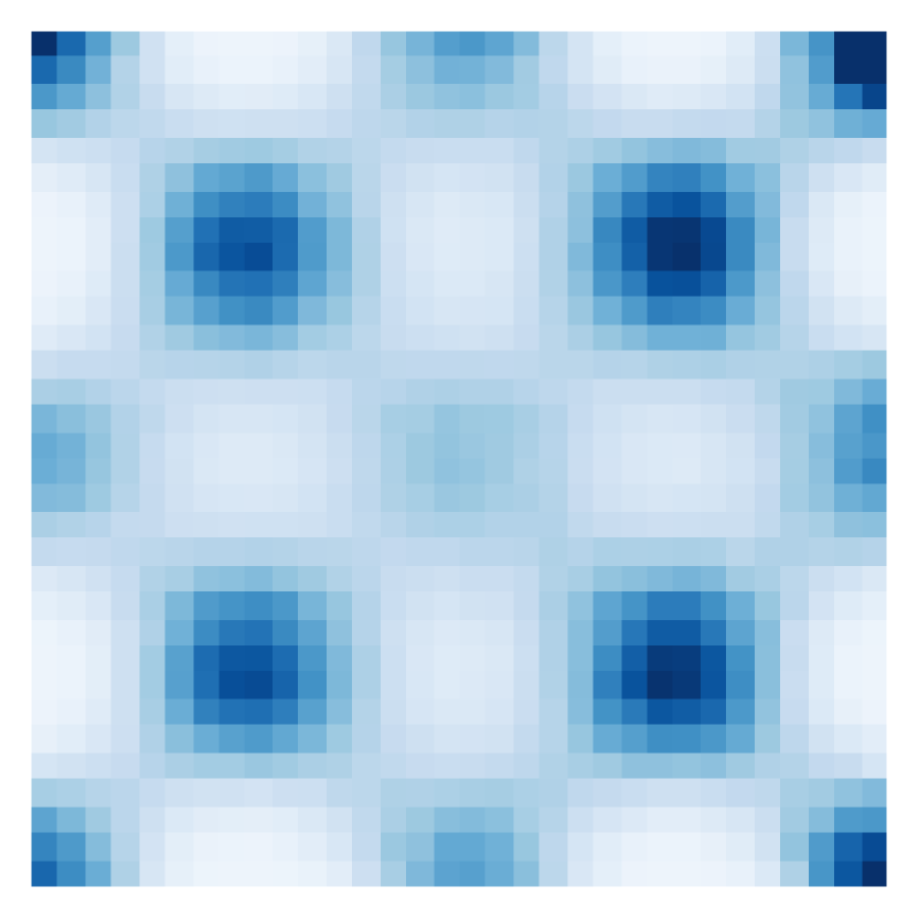
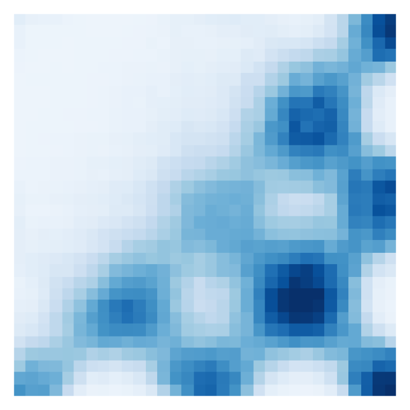
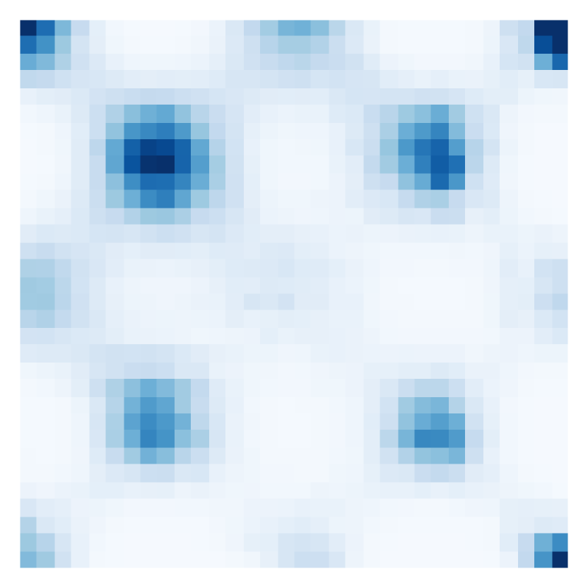
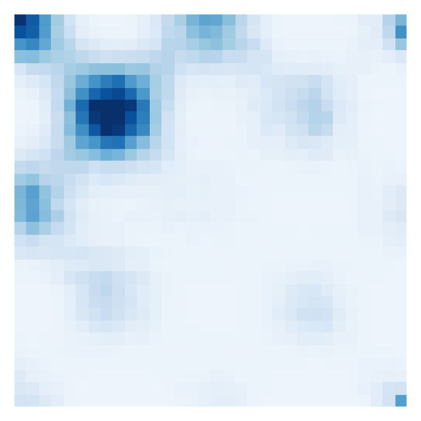
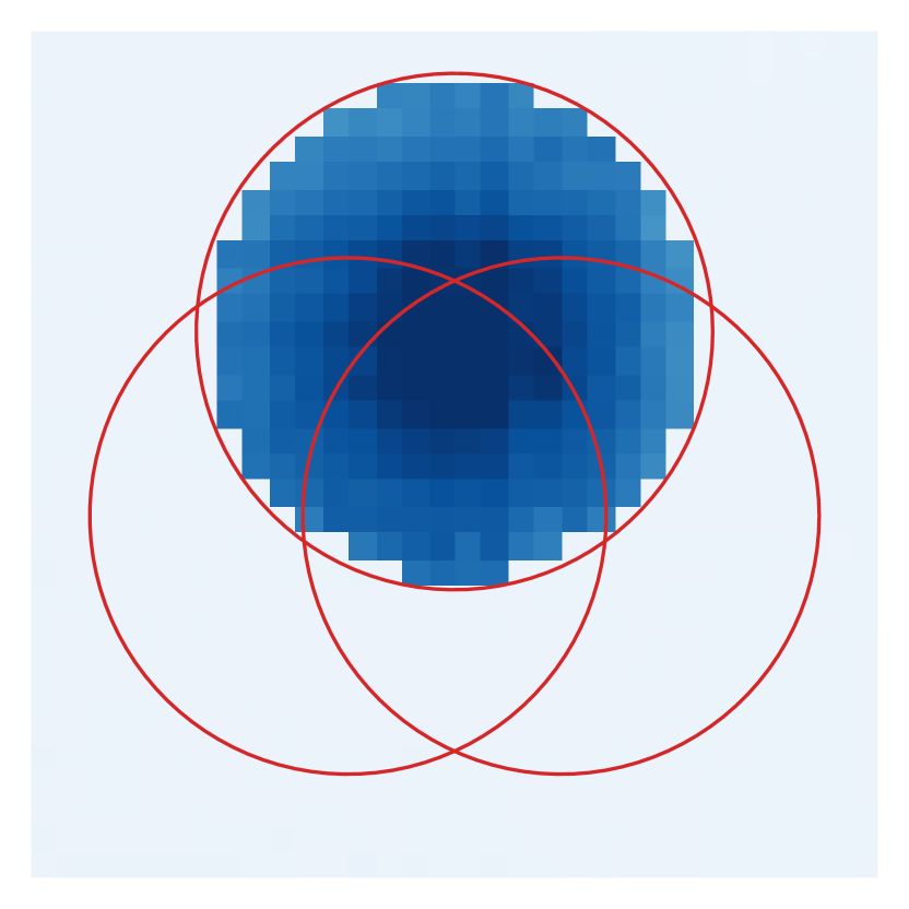
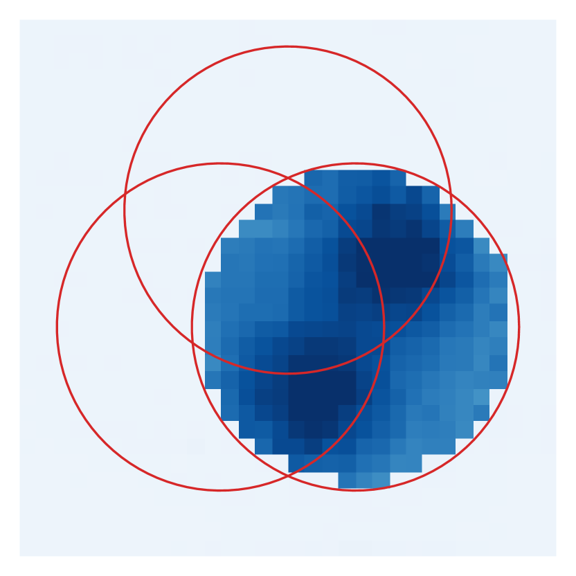
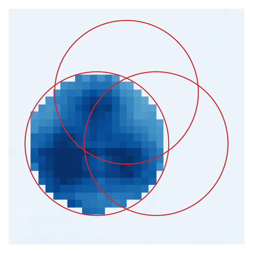
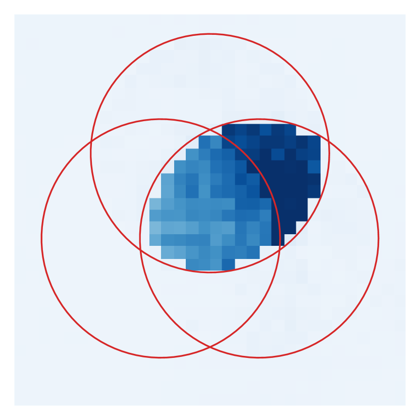
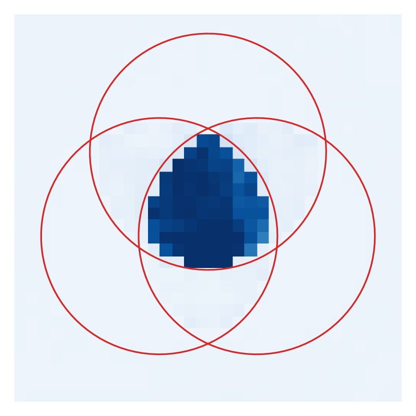
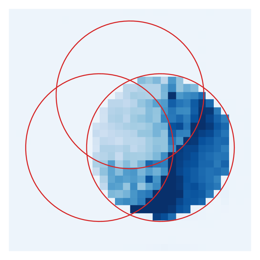
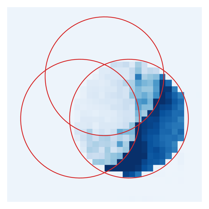
Figure 3: Composed GFlowNets on 32×32323232\times 32 grid domain. Color indicates cell probability, darker is higher. (Top) operations on two distributions. (Bottom) operations on three distributions. The red circles indicate the high probability regions of p1subscript𝑝1p_{1}, p2subscript𝑝2p_{2}, p3subscript𝑝3p_{3}.
Refer to caption
(a) Base at β=32𝛽32\beta=32
Refer to caption
(b) Harmonic mean
Refer to caption
(c) Contrasts
Refer to caption
(d) Base at β=96𝛽96\beta=96
Refer to caption
(e) Harmonic mean
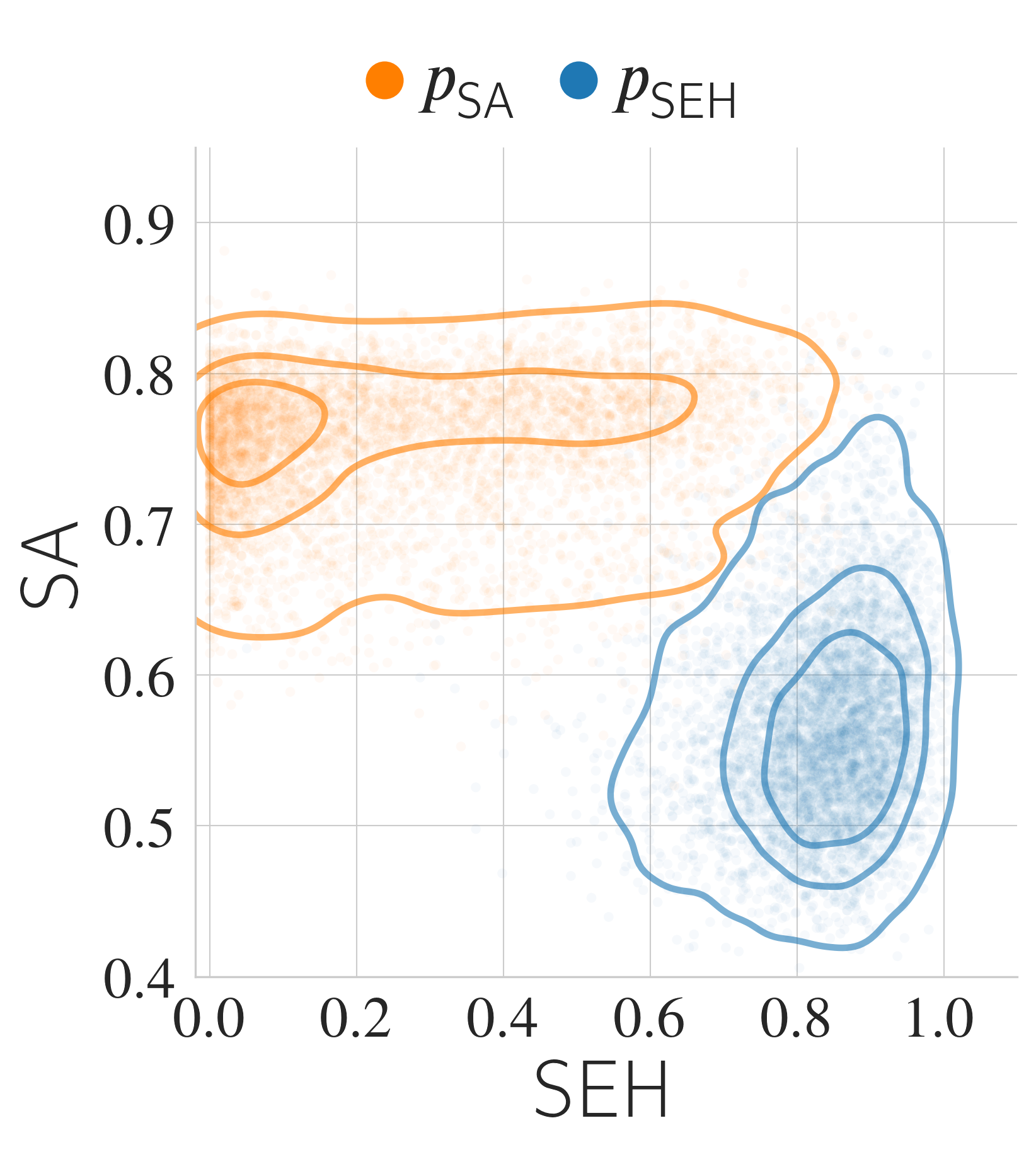
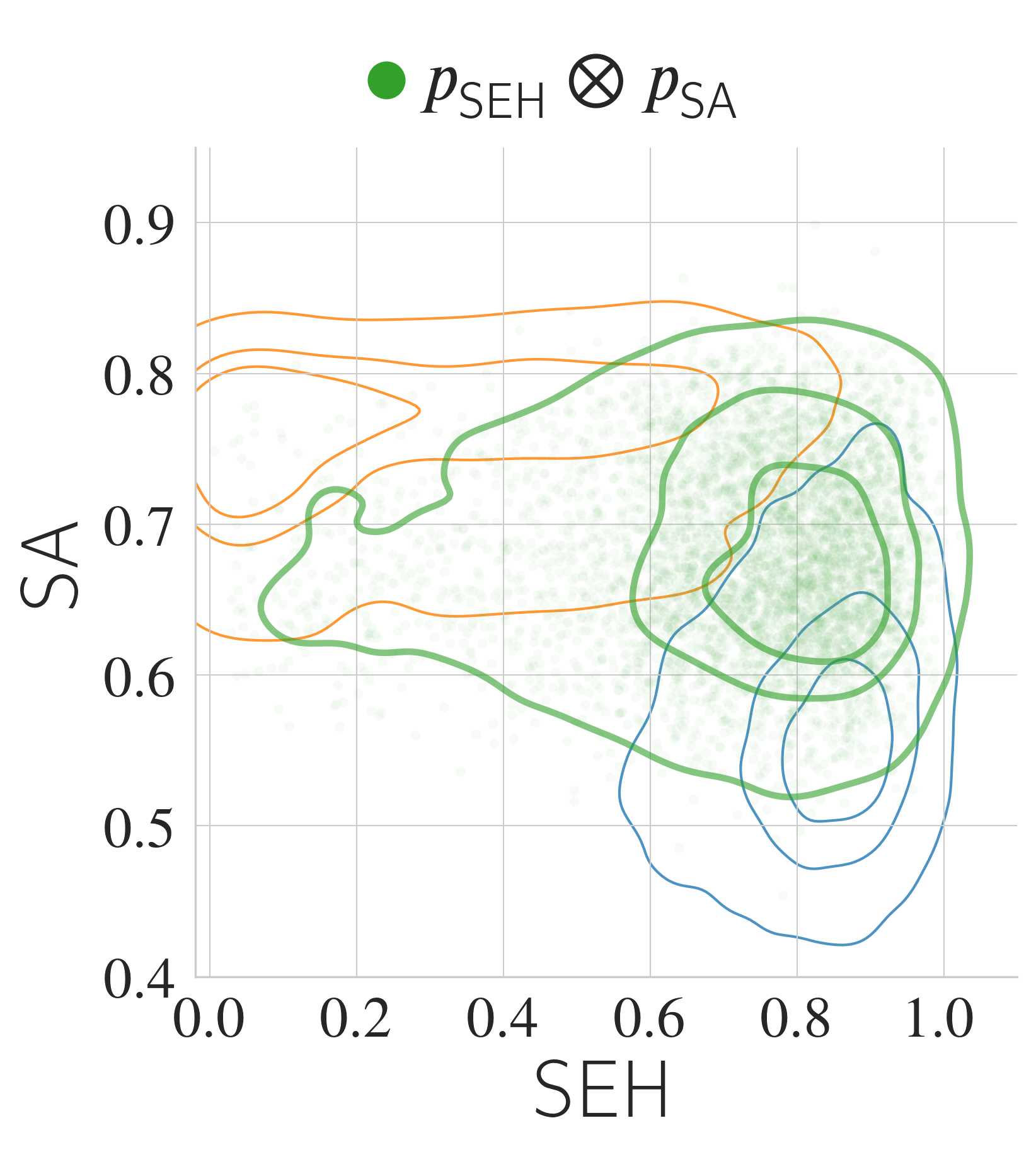
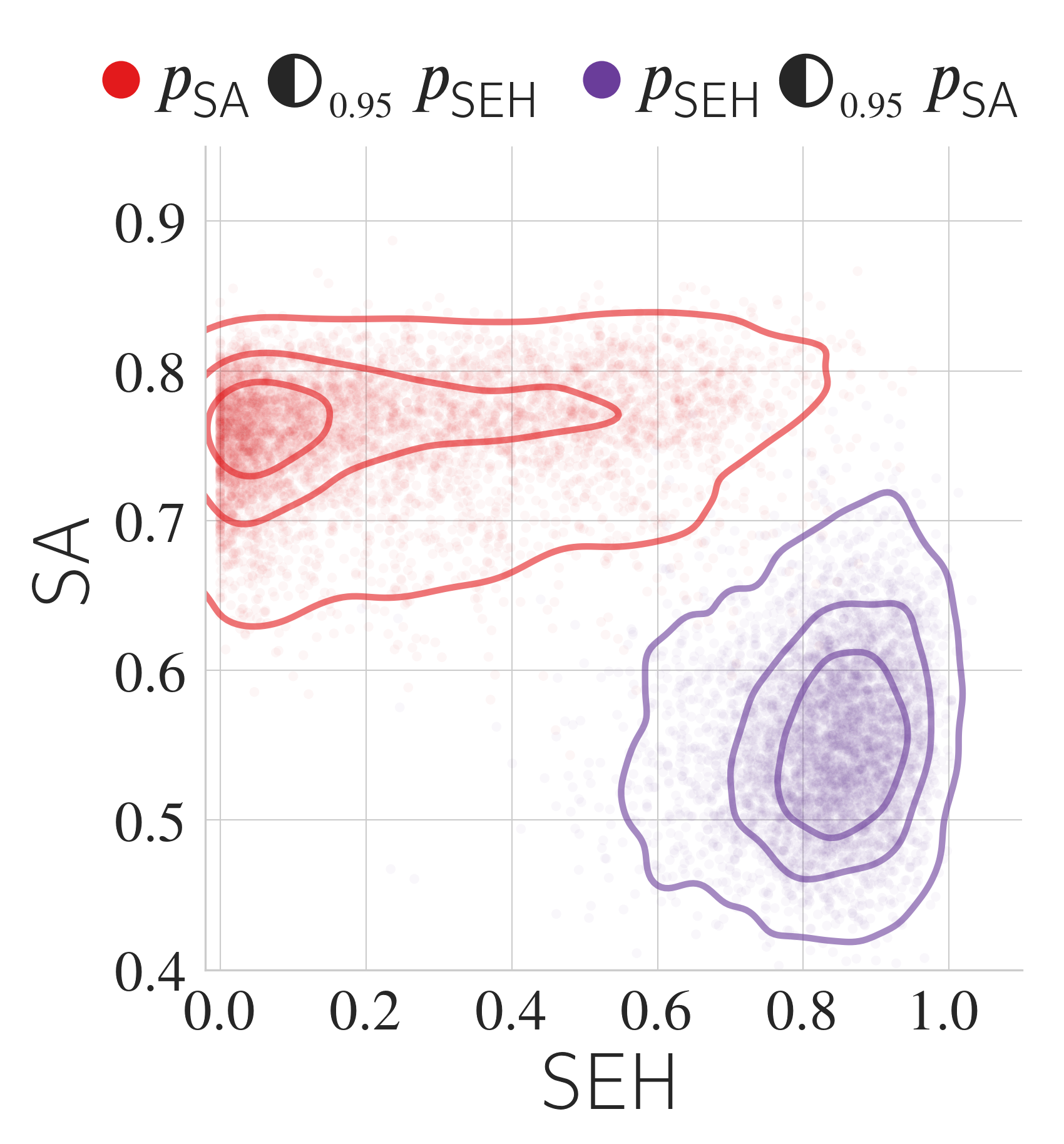
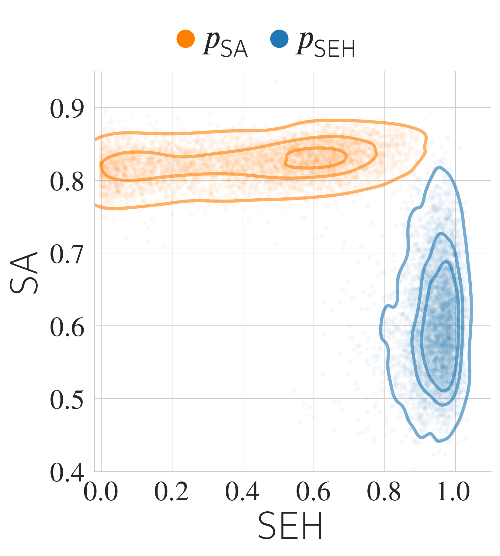
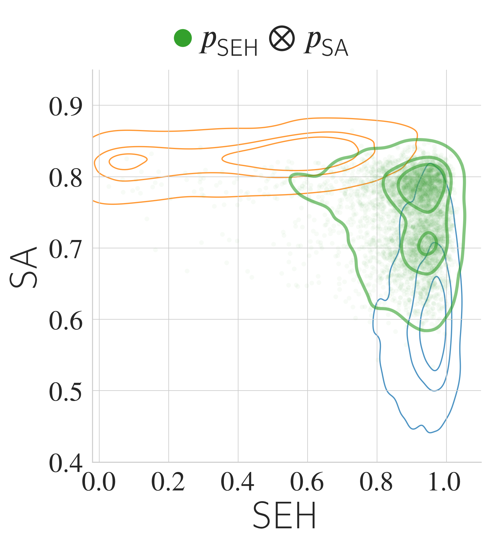
Figure 4: Reward distributions in the molecular generation domain. (a) Base GFlowNets at β=32𝛽32\beta\!=\!32: pSEHsubscript𝑝SEHp_{\text{SEH}} and pSAsubscript𝑝SAp_{\text{SA}} are trained with RSEH(x)32subscript𝑅SEHsuperscript𝑥32R_{\text{SEH}}(x)^{32} and RSA(x)32subscript𝑅SAsuperscript𝑥32R_{\text{SA}}(x)^{32}. (b) harmonic mean of pSEHsubscript𝑝SEHp_{\text{SEH}} and pSAsubscript𝑝SAp_{\text{SA}}, (c) contrasts. (d) base GFlowNets at β=96𝛽96\beta\!=\!96. (e) harmonic mean. The contours indicate the level sets of the kernel density estimates in the (RSEH,RSA)subscript𝑅SEHsubscript𝑅SA(R_{\text{SEH}},R_{\text{SA}}) plane.

6.1 2D Distributions via GFlowNet

We validate GFlowNet compositions obtained with our framework on 2D grid domain [36]. The goal of this experiment is to validate our approach in a controlled setting, where the ground-truth composite distributions can be evaluated directly.

In the 2D grid domain, the states are the cells of an H×H𝐻𝐻H\times H grid. The starting state is the upper-left cell s0=(0,0)subscript𝑠000s_{0}=(0,0). At each state, the allowed actions are: 1) move right; 2) move down; 3) a stop action that indicates termination of the trajectory at the current position. For this experiment, we first trained GFlowNets pi(x)Ri(x)proportional-tosubscript𝑝𝑖𝑥subscript𝑅𝑖𝑥p_{i}(x)\varpropto R_{i}(x) with reward functions Ri(x)>0subscript𝑅𝑖𝑥0R_{i}(x)>0 defined on the grid, and then trained classifiers and constructed GFlowNet compositions following 5.3.

Figure 3 (top row) shows the distributions obtained by composing two pre-trained GFlowNets (top row; left). The harmonic mean p1p2tensor-productsubscript𝑝1subscript𝑝2p_{1}\otimes p_{2}, covers the regions that have high probability under both p1subscript𝑝1p_{1} and p2subscript𝑝2p_{2} and excludes locations where either of the distributions is low. p1\circlerighthalfblackp2subscript𝑝1\circlerighthalfblacksubscript𝑝2p_{1}{\,\circlerighthalfblack\,}p_{2} resembles p1subscript𝑝1p_{1} but the relative masses of the modes of p1subscript𝑝1p_{1} are modulated by p2subscript𝑝2p_{2}: regions with high p2subscript𝑝2p_{2} have lower probability under contrast. The parameterized contrast p1\circlerighthalfblack0.95p2subscript𝑝1subscript\circlerighthalfblack0.95subscript𝑝2p_{1}{\,\circlerighthalfblack\,}_{0.95}\;p_{2} with α=0.05𝛼0.05\alpha=0.05 magnifies the contrasting effect: high p2(x)subscript𝑝2𝑥p_{2}(x) implies very low (p1\circlerighthalfblack0.95p2)(x)subscript𝑝1subscript\circlerighthalfblack0.95subscript𝑝2𝑥(p_{1}{\,\circlerighthalfblack\,}_{0.95}\;p_{2})(x).

The bottom row of Figure 3 shows the operations on 3 distributions. The conditional p~(x|y1=1,y2=2)~𝑝formulae-sequenceconditional𝑥subscript𝑦11subscript𝑦22\widetilde{p}(x|y_{1}\!=\!1,y_{2}\!=\!2) is concentrated on the points that have high likelihood under both p1subscript𝑝1p_{1} and p2subscript𝑝2p_{2}. Similarly, the value p~(x|y1=1,y2=2,y3=3)~𝑝formulae-sequenceconditional𝑥subscript𝑦11formulae-sequencesubscript𝑦22subscript𝑦33\widetilde{p}(x|y_{1}\!=\!1,y_{2}\!=\!2,y_{3}\!=\!3) is high if x𝑥x is likely to be observed under all three distributions at the same time. The conditionals p~(x|y1=2,y2=2)~𝑝formulae-sequenceconditional𝑥subscript𝑦12subscript𝑦22\widetilde{p}(x|y_{1}\!=\!2,y_{2}\!=\!2) and p~(x|y1=2,y2=2,y3=2)~𝑝formulae-sequenceconditional𝑥subscript𝑦12formulae-sequencesubscript𝑦22subscript𝑦32\widetilde{p}(x|y_{1}\!=\!2,y_{2}\!=\!2,y_{3}\!=\!2) highlight the points with high p2(x)subscript𝑝2𝑥p_{2}(x) but low p1(x)subscript𝑝1𝑥p_{1}(x) and p(x)p_{(}x). Conditioning on three labels results in a sharper distribution compared to double-conditioning. Note that the operations can be thought of as generalized set-theoretic operations (set intersection and set difference). We provide quantitative results and further details in Appendix E.1. The classifier learning curves are provided in Appendix F.4.

6.2 Molecule Generation via GFlowNet

Next, we evaluate our method for GFlowNet composition on a large and highly structured data space, and asses the effect that composition operations have on resulting data distributions in a practical setting. To that end, we conducted experiments with GFlowNets trained for the molecular generation task proposed by Bengio et al. [36].

Domain.

In the molecule generation task, the objects x𝒳𝑥𝒳x\in\mathcal{X} are molecular graphs. The non-terminal states s𝒮𝒳𝑠𝒮𝒳s\in\mathcal{S}\setminus\mathcal{X} are incomplete molecular graphs. The transitions from a given non-terminal state s𝑠s are of two types: 1) fragment addition ss𝑠superscript𝑠s\to s^{\prime}: new molecular graph ssuperscript𝑠s^{\prime} is obtained by attaching a new fragment to the molecular graph s𝑠s; 2) stop action sx𝑠𝑥s\to x: if ss0𝑠subscript𝑠0s\neq s_{0}, then the generation process can be terminated at the molecular graph corresponding to the current state (note that new terminal state x𝒳𝑥𝒳x\in\mathcal{X} is different from s𝒮𝒳𝑠𝒮𝒳s\in\mathcal{S}\setminus\mathcal{X}, but both states correspond to the same molecular graph).

Rewards.

We trained GFlowNets using 3 reward functions: SEH, a reward computed by an MPNN [56] that was trained by Bengio et al. [36] to estimate the binding energy of a molecule to the soluble epoxide hydrolase protein; SA, an estimate of synthetic accessibility [57] computed with tools from RDKit library [58]; QED, a quantitative estimate of drug-likeness [59] which is also computed with RDKit. We normalized all reward functions to the range [0,1]01[0,1]. Higher values of SEH, SA, and QED correspond to stronger binding, higher synthetic accessibility, and higher drug-likeness respectively. Following Bengio et al. [36], we introduced the parameter β𝛽\beta which controls the sharpness (temperature) of the target distribution: p(x)R(x)βproportional-to𝑝𝑥𝑅superscript𝑥𝛽p(x)\varpropto R(x)^{\beta}, increasing β𝛽\beta results in a distribution skewed towards high-reward objects. We experimented with two β𝛽\beta values, 323232 and 969696 (Figure 4(a),4(d)).

Training and evaluation.

After training the base GFlowNets with the reward functions described above, we trained classifiers with Algorithm 1. The classifier was parameterized as a graph neural network based on a graph transformer architecture [60]. Further details of the classifier parameterization and training are provided in Appendix E.2. Compared to the 2D grid domain (Section 6.1), we can not directly evaluate the distributions obtained by our approach. Instead, we analyzed the samples generated by the composed distributions. We sampled 5 00050005\,000 molecules from each composed distribution obtained with our approach as well as the base GFlowNets. We evaluated the sample collections with the two following strategies. Reward evaluation: we analyzed the distributions of rewards across the sample collections. The goal is to see whether the composition of GFlowNets trained for different rewards leads to noticeable changes in reward distribution. Distribution distance evaluation: we used the samples to estimate the pairwise distances between the distributions. Specifically, for a given pair of distributions represented by two collections of samples 𝒟A={xA,i}i=1nsubscript𝒟𝐴superscriptsubscriptsubscript𝑥𝐴𝑖𝑖1𝑛\mathcal{D}_{A}=\{x_{A,i}\}_{i=1}^{n}, 𝒟B={xB,i}i=1nsubscript𝒟𝐵superscriptsubscriptsubscript𝑥𝐵𝑖𝑖1𝑛\mathcal{D}_{B}=\{x_{B,i}\}_{i=1}^{n} we computed the earth mover’s distance d(𝒟A,𝒟B)𝑑subscript𝒟𝐴subscript𝒟𝐵d(\mathcal{D}_{A},\mathcal{D}_{B}) with ground molecule distance given by d(x,x)=(max{s(x,x),103})11𝑑𝑥superscript𝑥superscript𝑠𝑥superscript𝑥superscript10311d(x,x^{\prime})=(\max\{s(x,x^{\prime}),10^{-3}\})^{-1}-1, where s(x,x)[0,1]𝑠𝑥superscript𝑥01s(x,x^{\prime})\in[0,1] is the Tanimoto similarity over Morgan fingerprints of molecules x𝑥x and xsuperscript𝑥x^{\prime}.

Figure 5: Reward distributions of composite GFlowNets.
SEH low high
SA low high low high
QED low high low high low high low high
pSEHsubscript𝑝SEHp_{\text{SEH}} 0 0 0 0 𝟔𝟐62\bm{62} 𝟗9\bm{9} 𝟐𝟒24\bm{24} 𝟓5\bm{5}
pSAsubscript𝑝SAp_{\text{SA}} 0 0 𝟕𝟑73\bm{73} 𝟒4\bm{4} 0 0 𝟏𝟖18\bm{18} 𝟓5\bm{5}
pQEDsubscript𝑝QEDp_{\text{QED}} 0 𝟒𝟎40\bm{40} 0 𝟐𝟔26\bm{26} 0 𝟐𝟏21\bm{21} 0 𝟏𝟑13\bm{13}
(a) y={SEH,SA}𝑦SEHSAy\!=\!\{{\text{SEH},\text{SA}}\} 1 0 16 2 6 3 𝟓𝟒54\bm{54} 𝟏𝟖18\bm{18}
(b) y={SEH,QED}𝑦SEHQEDy\!=\!\{{\text{SEH},\text{QED}}\} 0 11 0 4 1 𝟒𝟖48\bm{48} 4 𝟑𝟐32\bm{32}
(c) y={SA,QED}𝑦SAQEDy\!=\!\{{\text{SA},\text{QED}}\} 0 15 1 𝟒𝟐42\bm{42} 0 8 2 𝟑𝟐32\bm{32}
(d) y={SEH,SA,QED}𝑦SEHSAQEDy\!=\!\{{\text{SEH},\text{SA},\text{QED}}\} 0 7 2 11 2 19 10 𝟒𝟗49\bm{49}
(e) y={SEH,SEH,SEH}𝑦SEHSEHSEHy\!=\!\{{\text{SEH},\text{SEH},\text{SEH}}\} 0 0 0 0 𝟔𝟑63\bm{63} 9 24 4
(f) y={SA,SA,SA}𝑦SASASAy\!=\!\{{\text{SA},\text{SA},\text{SA}}\} 0 0 𝟕𝟒74\bm{74} 5 0 0 17 4
(g) y={QED,QED,QED}𝑦QEDQEDQEDy\!=\!\{{\text{QED},\text{QED},\text{QED}}\} 0 𝟒𝟎40\bm{40} 0 23 0 23 0 14

In each row, the numbers show the percentage of the samples from the respective model that fall into one of 888 bins according to rewards. The “low” and “high” categories are decided by thresholding SEH: 0.5, SA: 0.6, QED: 0.25.
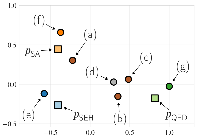
Refer to caption
Figure 6: 2D t-SNE embeddings of three base GFlowNets trained with RSEH(x)βsubscript𝑅SEHsuperscript𝑥𝛽R_{\text{SEH}}(x)^{\beta}, RSA(x)βsubscript𝑅SAsuperscript𝑥𝛽R_{\text{SA}}(x)^{\beta}, RQED(x)βsubscript𝑅QEDsuperscript𝑥𝛽R_{\text{QED}}(x)^{\beta}, at β=32𝛽32\beta\!=\!32 and their compositions. The t-SNE embeddings are computed based on pairwise earth mover’s distances between the distributions. Labels (a)-(g) match rows in Table 6.

Results.

Figure 4 shows reward distributions of base GFlowNets (trained with SEH and SA rewards at β{32,96})\beta\in\{32,96\}) and their compositions. Base GFlowNet distributions are concentrated on examples that score high in their respective rewards. For each model, there is considerable variation in the reward that was not used for training. The harmonic mean operation (Figures 4(b), 4(e)) results in distributions that are concentrated on the samples scoring high in both rewards. The contrast operation (Figure 4(c)) has the opposite effect: the distributions are skewed towards the examples scoring high in only one of the original rewards. Note that the tails of the contrast distributions are retreating from the area covered by the harmonic mean.

We show reward distribution statistics of three GFlowNets (trained with SEH, SA, and QED at β=32𝛽32\beta=32) and their compositions in Table 6. Each row of the table gives a breakdown (percentages) of the samples from a given model into one of 23=8superscript2382^{3}=8 bins according to rewards. For all three base models, the majority of the samples fall into the “high” category according to the respective reward, while the rewards that were not used for training show variation. Conditioning on two different labels (e.g. y={SEH,QED}𝑦SEHQEDy\!=\!\{\text{SEH},\text{QED}\}) results in concentration on examples that score high in two selected rewards, but not necessarily scoring high in the reward that was not selected. The conditional y={SEH,QED,SA}𝑦SEHQEDSAy\!=\!\{\text{SEH},\text{QED},\text{SA}\} shifts the focus to examples that have all three properties.

Figure 6 shows 2D embeddings of the distributions appearing in Table 6. The embeddings were computed with t-SNE based on the pairwise earth mover’s distances. The configuration of the embeddings gives insight into the configuration of base models and conditionals in the distribution space. We see that points corresponding to pairwise conditionals lie in between the two base models selected for conditioning. Conditional y={SEH,SA,QED}𝑦SEHSAQEDy\!=\!\{\text{SEH},\text{SA},\text{QED}\} appears to be near the centroid of the triangle (pSEH,pSA,pQED)subscript𝑝SEHsubscript𝑝SAsubscript𝑝QED(p_{\text{SEH}},p_{\text{SA}},p_{\text{QED}}) and lies close the the pairwise conditoinals. The distributions obtained by repeated conditioning on the same label value (e.g. y={SEH,SEH,SEH}𝑦SEHSEHSEHy\!=\!\{\text{SEH},\text{SEH},\text{SEH}\}) are spread out to the boundary and lie closer to the respective base distributions while being relatively far from pairwise conditionals. We provide a complete summary of the distribution distances in Table F.1. The classifier learning curves are provided in Appendix F.4. The sample diversity statistics of base GFlowNets at different values of β𝛽\beta are provided in Appendix F.5.

6.3 Colored MNIST Generation via Diffusion Models
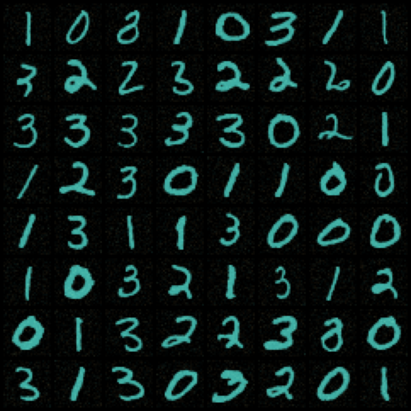
Refer to caption
p1subscript𝑝1p_{1}\vphantom{\widetilde{p}\left(\!x\middle|\begin{subarray}{c}y_{1}=1\\ y_{2}=2\\ y_{3}=3\end{subarray}\right)}
Refer to caption
p2subscript𝑝2p_{2}\vphantom{\widetilde{p}\left(\!x\middle|\begin{subarray}{c}y_{1}=1\\ y_{2}=2\\ y_{3}=3\end{subarray}\right)}
Refer to caption
p3subscript𝑝3p_{3}\vphantom{\widetilde{p}\left(\!x\middle|\begin{subarray}{c}y_{1}=1\\ y_{2}=2\\ y_{3}=3\end{subarray}\right)}
Refer to caption
p~(x|y1=1y2=1)\widetilde{p}\left(\!x\middle|\begin{subarray}{c}y_{1}=1\\ y_{2}=1\end{subarray}\right)\vphantom{\widetilde{p}\left(\!x\middle|\begin{subarray}{c}y_{1}=1\\ y_{2}=1\\ y_{3}=3\end{subarray}\right)}
Refer to caption
p~(x|y1=2y2=2)\widetilde{p}\left(\!x\middle|\begin{subarray}{c}y_{1}=2\\ y_{2}=2\end{subarray}\right)\vphantom{\widetilde{p}\left(\!x\middle|\begin{subarray}{c}y_{1}=2\\ y_{2}=2\\ y_{3}=3\end{subarray}\right)}
Refer to caption
p~(x|y1=3y2=3)\widetilde{p}\left(\!x\middle|\begin{subarray}{c}y_{1}=3\\ y_{2}=3\end{subarray}\right)\vphantom{\widetilde{p}\left(\!x\middle|\begin{subarray}{c}y_{1}=1\\ y_{2}=2\\ y_{3}=3\end{subarray}\right)}
Refer to caption
p~(x|y1=1y2=2)\widetilde{p}\left(\!x\middle|\begin{subarray}{c}y_{1}=1\\ y_{2}=2\end{subarray}\right)\vphantom{\widetilde{p}\left(\!x\middle|\begin{subarray}{c}y_{1}=1\\ y_{2}=2\\ y_{3}=3\end{subarray}\right)}
Refer to caption
p~(x|y1=1y2=3)\widetilde{p}\left(\!x\middle|\begin{subarray}{c}y_{1}=1\\ y_{2}=3\end{subarray}\right)\vphantom{\widetilde{p}\left(\!x\middle|\begin{subarray}{c}y_{1}=1\\ y_{2}=2\\ y_{3}=3\end{subarray}\right)}
Refer to caption
p~(x|y1=2y2=3)\widetilde{p}\left(\!x\middle|\begin{subarray}{c}y_{1}=2\\ y_{2}=3\end{subarray}\right)\vphantom{\widetilde{p}\left(\!x\middle|\begin{subarray}{c}y_{1}=1\\ y_{2}=2\\ y_{3}=3\end{subarray}\right)}
Refer to caption
p~(x|y1=1y2=2y3=3)\widetilde{p}\left(\!x\middle|\begin{subarray}{c}y_{1}=1\\ y_{2}=2\\ y_{3}=3\end{subarray}\right)
Refer to caption
p~(x|y1=1y2=2y3=1)\widetilde{p}\left(\!x\middle|\begin{subarray}{c}y_{1}=1\\ y_{2}=2\\ y_{3}=1\end{subarray}\right)
Refer to caption
p~(x|y1=1y2=2y3=2)\widetilde{p}\left(\!x\middle|\begin{subarray}{c}y_{1}=1\\ y_{2}=2\\ y_{3}=2\end{subarray}\right)
Figure 7: Composed diffusion models on colored MNIST. Samples from 3 pre-trained diffusion models and their various compositions.

Finally, we empirically test our method for the composition of diffusion models on image generation task.

In this experiment, we composed three diffusion models that are pre-trained to generate colored MNIST digits [61]. Model p1subscript𝑝1p_{1} was trained to generate cyan digits less than 4, p2subscript𝑝2p_{2} to generate cyan and beige digits less than 2, and p3subscript𝑝3p_{3} to generate cyan and beige even digits less than 4. In essence, each model was trained to generate digits with a specific property: p1subscript𝑝1p_{1} generates cyan digits, p2subscript𝑝2p_{2} generates digits less than 2, and p3subscript𝑝3p_{3} generates even digits.

We built the composition iteratively by factorizing the posterior as p~(x|y1,y2,y3)p~(x)p~(y1,y2|x)p~(y3|x,y1,y2)proportional-to~𝑝conditional𝑥subscript𝑦1subscript𝑦2subscript𝑦3~𝑝𝑥~𝑝subscript𝑦1conditionalsubscript𝑦2𝑥~𝑝conditionalsubscript𝑦3𝑥subscript𝑦1subscript𝑦2\widetilde{p}(x|y_{1},y_{2},y_{3})\propto\widetilde{p}(x)\widetilde{p}(y_{1},y_{2}|x)\widetilde{p}(y_{3}|x,y_{1},y_{2}). To this end, we first trained a classifier Q~(y1,y2|xt)~𝑄subscript𝑦1conditionalsubscript𝑦2subscript𝑥𝑡\widetilde{Q}(y_{1},y_{2}|x_{t}) on trajectories sampled from the base models. This allows us to generate samples from p~(x|y1,y2)~𝑝conditional𝑥subscript𝑦1subscript𝑦2\widetilde{p}(x|y_{1},y_{2}). We then trained an additional classifier Q~(y3|xt,y1,y2)~𝑄conditionalsubscript𝑦3subscript𝑥𝑡subscript𝑦1subscript𝑦2\widetilde{Q}(y_{3}|x_{t},y_{1},y_{2}) on trajectories from compositions defined by (y1,y2)subscript𝑦1subscript𝑦2(y_{1},y_{2}) to allow us to sample from p~(x|y1,y2,y3)~𝑝conditional𝑥subscript𝑦1subscript𝑦2subscript𝑦3\widetilde{p}(x|y_{1},y_{2},y_{3}). Additional details can be found in Appendix E.3.

Figure 7 shows samples from the pre-trained models and from selected compositions. The negating effect of not conditioning on observations is clearly visible in the compositions using two variables. For example, p~(x|y1=1,y2=1)~𝑝formulae-sequenceconditional𝑥subscript𝑦11subscript𝑦21\widetilde{p}(x|y_{1}\!=\!1,y_{2}\!=\!1) only generates cyan 3 digits. Because there we do not condition on p2subscript𝑝2p_{2} or p3subscript𝑝3p_{3}, the composition excludes digits that have high probability under p2subscript𝑝2p_{2} or p3subscript𝑝3p_{3}, i.e. those that are less than 2 or even. We can make a similar analysis of p~(x|y1=1,y2=3)~𝑝formulae-sequenceconditional𝑥subscript𝑦11subscript𝑦23\widetilde{p}(x|y_{1}\!=\!1,y_{2}\!=\!3). Cyan even digits have high density under both p1subscript𝑝1p_{1} and p3subscript𝑝3p_{3}, but because p2subscript𝑝2p_{2} is not conditioned on, the composition excludes digits less than two (i.e. cyan 0’s). Finally, p~(x|y1=1,y2=2,y3=3)~𝑝formulae-sequenceconditional𝑥subscript𝑦11formulae-sequencesubscript𝑦22subscript𝑦33\widetilde{p}(x|y_{1}\!=\!1,y_{2}\!=\!2,y_{3}\!=\!3) generates only cyan 0 digits, on which all base models have high density.

7 Conclusion

We introduced Compositional Sculpting, a general approach for composing iterative generative models. Compositions are defined through “observations”, which enable us to emphasize or de-emphasize the density of the composition in regions where specific base models have high density. We highlighted two binary compositions, harmonic mean and contrast, which are analogous to the product and negation operations defined on EBMs. A crucial feature of the compositions we have introduced is that we can sample from them directly. By extending classifier guidance we are able to leverage the generative capabilities of the base models to produce samples from the composition. Through empirical experiments, we validated our approach for composing diffusion models and GFlowNets on toy domains, molecular generation, and image generation.

Acknowledgements

TG and TJ acknowledge support from the Machine Learning for Pharmaceutical Discovery and Synthesis (MLPDS) consortium, DARPA Accelerated Molecular Discovery program, the NSF Expeditions grant (award 1918839) "Understanding the World Through Code", and from the MIT-DSTA collaboration.

SK and SDP were supported by the Technology Industries of Finland Centennial Foundation and the Jane and Aatos Erkko Foundation under project Interactive Artificial Intelligence for Driving R&D, the Academy of Finland (flagship programme: Finnish Center for Artificial Intelligence, FCAI; grants 328400, 345604 and 341763), and the UKRI Turing AI World-Leading Researcher Fellowship, EP/W002973/1.

VG acknowledges support from the Academy of Finland (grant decision 342077) for "Human-steered next-generation machine learning for reviving drug design", the Saab-WASP initiative (grant 411025), and the Jane and Aatos Erkko Foundation (grant 7001703) for "Biodesign: Use of artificial intelligence in enzyme design for synthetic biology".

GY acknowledges support from the National Science Foundation under Cooperative Agreement PHY-2019786 (The NSF AI Institute for Artificial Intelligence and Fundamental Interactions, http://iaifi.org).

We thank Sammie Katt and Pavel Izmailov for the helpful discussions and assistance in making the figures.

We thank NeurIPS 2023 anonymous reviewers for the helpful feedback on our work.

Broader Impact

We proposed a mathematical framework and methods for the composition of pre-trained generative models. While the primary emphasis of our work is on advancing foundational research on generative modeling methodology and principled sampling techniques, our work inherits ethical concerns associated with generative models such as creation of deepfake content and misinformation dissemination, as well as reproduction of biases present in the datasets used for model training. If not carefully managed, these models can perpetuate societal biases, exacerbating issues of fairness and equity.

Our work contributes to research on the reuse of pre-trained models. This research direction promotes eco-friendly AI development, with the long-term goal of reducing energy consumption and carbon emissions associated with large-scale generative model training.

References

  • Kirillov et al. [2023] Alexander Kirillov, Eric Mintun, Nikhila Ravi, Hanzi Mao, Chloe Rolland, Laura Gustafson, Tete Xiao, Spencer Whitehead, Alexander C. Berg, Wan-Yen Lo, Piotr Dollár, and Ross B. Girshick. Segment anything. ArXiv, abs/2304.02643, 2023.
  • Radford et al. [2021] Alec Radford, Jong Wook Kim, Chris Hallacy, Aditya Ramesh, Gabriel Goh, Sandhini Agarwal, Girish Sastry, Amanda Askell, Pamela Mishkin, Jack Clark, et al. Learning transferable visual models from natural language supervision. In International conference on machine learning, pages 8748–8763. PMLR, 2021.
  • Cherti et al. [2023] Mehdi Cherti, Romain Beaumont, Ross Wightman, Mitchell Wortsman, Gabriel Ilharco, Cade Gordon, Christoph Schuhmann, Ludwig Schmidt, and Jenia Jitsev. Reproducible scaling laws for contrastive language-image learning. In Proceedings of the IEEE/CVF Conference on Computer Vision and Pattern Recognition, pages 2818–2829, 2023.
  • Rombach et al. [2022] Robin Rombach, Andreas Blattmann, Dominik Lorenz, Patrick Esser, and Björn Ommer. High-resolution image synthesis with latent diffusion models. In Proceedings of the IEEE/CVF Conference on Computer Vision and Pattern Recognition, pages 10684–10695, 2022.
  • Ho et al. [2020] Jonathan Ho, Ajay Jain, and Pieter Abbeel. Denoising diffusion probabilistic models. Advances in Neural Information Processing Systems, 33:6840–6851, 2020.
  • Ramesh et al. [2021] Aditya Ramesh, Mikhail Pavlov, Gabriel Goh, Scott Gray, Chelsea Voss, Alec Radford, Mark Chen, and Ilya Sutskever. Zero-shot text-to-image generation. In International Conference on Machine Learning, pages 8821–8831. PMLR, 2021.
  • Devlin et al. [2018] Jacob Devlin, Ming-Wei Chang, Kenton Lee, and Kristina Toutanova. Bert: Pre-training of deep bidirectional transformers for language understanding. ArXiv, abs/1810.04805, 2018.
  • Brown et al. [2020] Tom Brown, Benjamin Mann, Nick Ryder, Melanie Subbiah, Jared D Kaplan, Prafulla Dhariwal, Arvind Neelakantan, Pranav Shyam, Girish Sastry, Amanda Askell, et al. Language models are few-shot learners. Advances in neural information processing systems, 33:1877–1901, 2020.
  • OpenAI [2023] OpenAI. Chatgpt (mar 14 version). Large language model, 2023. URL https://chat.openai.com/chat.
  • Roberts et al. [2022] Adam Roberts, Hyung Won Chung, Anselm Levskaya, Gaurav Mishra, James Bradbury, Daniel Andor, Sharan Narang, Brian Lester, Colin Gaffney, Afroz Mohiuddin, Curtis Hawthorne, Aitor Lewkowycz, Alexandru Salcianu, Marc van Zee, Jacob Austin, Sebastian Goodman, Livio Baldini Soares, Haitang Hu, Sasha Tsvyashchenko, Aakanksha Chowdhery, Jasmijn Bastings, Jannis Bulian, Xavier García, Jianmo Ni, Andrew Chen, Kathleen Kenealy, J. Clark, Stephan Lee, Daniel H Garrette, James Lee-Thorp, Colin Raffel, Noam M. Shazeer, Marvin Ritter, Maarten Bosma, Alexandre Passos, Jeremy B. Maitin-Shepard, Noah Fiedel, Mark Omernick, Brennan Saeta, Ryan Sepassi, Alexander Spiridonov, Joshua Newlan, and Andrea Gesmundo. Scaling up models and data with t5x and seqio. ArXiv, abs/2203.17189, 2022.
  • Chowdhery et al. [2022] Aakanksha Chowdhery, Sharan Narang, Jacob Devlin, Maarten Bosma, Gaurav Mishra, Adam Roberts, Paul Barham, Hyung Won Chung, Charles Sutton, Sebastian Gehrmann, et al. Palm: Scaling language modeling with pathways. ArXiv, abs/2204.02311, 2022.
  • Brohan et al. [2022] Anthony Brohan, Noah Brown, Justice Carbajal, Yevgen Chebotar, Joseph Dabis, Chelsea Finn, Keerthana Gopalakrishnan, Karol Hausman, Alexander Herzog, Jasmine Hsu, Julian Ibarz, Brian Ichter, Alex Irpan, Tomas Jackson, Sally Jesmonth, Nikhil J. Joshi, Ryan C. Julian, Dmitry Kalashnikov, Yuheng Kuang, Isabel Leal, Kuang-Huei Lee, Sergey Levine, Yao Lu, Utsav Malla, Deeksha Manjunath, Igor Mordatch, Ofir Nachum, Carolina Parada, Jodilyn Peralta, Emily Perez, Karl Pertsch, Jornell Quiambao, Kanishka Rao, Michael S. Ryoo, Grecia Salazar, Pannag R. Sanketi, Kevin Sayed, Jaspiar Singh, Sumedh Anand Sontakke, Austin Stone, Clayton Tan, Huong Tran, Vincent Vanhoucke, Steve Vega, Quan Ho Vuong, F. Xia, Ted Xiao, Peng Xu, Sichun Xu, Tianhe Yu, and Brianna Zitkovich. Rt-1: Robotics transformer for real-world control at scale. ArXiv, abs/2212.06817, 2022.
  • Driess et al. [2023] Danny Driess, F. Xia, Mehdi S. M. Sajjadi, Corey Lynch, Aakanksha Chowdhery, Brian Ichter, Ayzaan Wahid, Jonathan Tompson, Quan Ho Vuong, Tianhe Yu, Wenlong Huang, Yevgen Chebotar, Pierre Sermanet, Daniel Duckworth, Sergey Levine, Vincent Vanhoucke, Karol Hausman, Marc Toussaint, Klaus Greff, Andy Zeng, Igor Mordatch, and Peter R. Florence. Palm-e: An embodied multimodal language model. ArXiv, abs/2303.03378, 2023.
  • Ahn et al. [2023] Michael Ahn, Anthony Brohan, Noah Brown, Yevgen Chebotar, Omar Cortes, Byron David, Chelsea Finn, Chuyuan Fu, Keerthana Gopalakrishnan, Karol Hausman, Alexander Herzog, Daniel Ho, Jasmine Hsu, Julian Ibarz, Brian Ichter, Alex Irpan, Eric Jang, Rosario Jauregui Ruano, Kyle Jeffrey, Sally Jesmonth, Nikhil Jayant Joshi, Ryan C. Julian, Dmitry Kalashnikov, Yuheng Kuang, Kuang-Huei Lee, Sergey Levine, Yao Lu, Linda Luu, Carolina Parada, Peter Pastor, Jornell Quiambao, Kanishka Rao, Jarek Rettinghouse, Diego M Reyes, Pierre Sermanet, Nicolas Sievers, Clayton Tan, Alexander Toshev, Vincent Vanhoucke, Fei Xia, Ted Xiao, Peng Xu, Sichun Xu, Mengyuan Yan, and Andy Zeng. Do as i can, not as i say: Grounding language in robotic affordances. In Karen Liu, Dana Kulic, and Jeff Ichnowski, editors, Proceedings of The 6th Conference on Robot Learning, volume 205 of Proceedings of Machine Learning Research, pages 287–318. PMLR, 2023.
  • Jumper et al. [2021] John Jumper, Richard Evans, Alexander Pritzel, Tim Green, Michael Figurnov, Olaf Ronneberger, Kathryn Tunyasuvunakool, Russ Bates, Augustin Žídek, Anna Potapenko, et al. Highly accurate protein structure prediction with alphafold. Nature, 596(7873):583–589, 2021.
  • Bommasani et al. [2021] Rishi Bommasani, Drew A. Hudson, Ehsan Adeli, Russ Altman, Simran Arora, Sydney von Arx, Michael S. Bernstein, Jeannette Bohg, Antoine Bosselut, Emma Brunskill, Erik Brynjolfsson, S. Buch, Dallas Card, Rodrigo Castellon, Niladri S. Chatterji, Annie S. Chen, Kathleen A. Creel, Jared Davis, Dora Demszky, Chris Donahue, Moussa Doumbouya, Esin Durmus, Stefano Ermon, John Etchemendy, Kawin Ethayarajh, Li Fei-Fei, Chelsea Finn, Trevor Gale, Lauren E. Gillespie, Karan Goel, Noah D. Goodman, Shelby Grossman, Neel Guha, Tatsunori Hashimoto, Peter Henderson, John Hewitt, Daniel E. Ho, Jenny Hong, Kyle Hsu, Jing Huang, Thomas F. Icard, Saahil Jain, Dan Jurafsky, Pratyusha Kalluri, Siddharth Karamcheti, Geoff Keeling, Fereshte Khani, O. Khattab, Pang Wei Koh, Mark S. Krass, Ranjay Krishna, Rohith Kuditipudi, Ananya Kumar, Faisal Ladhak, Mina Lee, Tony Lee, Jure Leskovec, Isabelle Levent, Xiang Lisa Li, Xuechen Li, Tengyu Ma, Ali Malik, Christopher D. Manning, Suvir Mirchandani, Eric Mitchell, Zanele Munyikwa, Suraj Nair, Avanika Narayan, Deepak Narayanan, Benjamin Newman, Allen Nie, Juan Carlos Niebles, Hamed Nilforoshan, J. F. Nyarko, Giray Ogut, Laurel J. Orr, Isabel Papadimitriou, Joon Sung Park, Chris Piech, Eva Portelance, Christopher Potts, Aditi Raghunathan, Robert Reich, Hongyu Ren, Frieda Rong, Yusuf H. Roohani, Camilo Ruiz, Jack Ryan, Christopher R’e, Dorsa Sadigh, Shiori Sagawa, Keshav Santhanam, Andy Shih, Krishna Parasuram Srinivasan, Alex Tamkin, Rohan Taori, Armin W. Thomas, Florian Tramèr, Rose E. Wang, William Wang, Bohan Wu, Jiajun Wu, Yuhuai Wu, Sang Michael Xie, Michihiro Yasunaga, Jiaxuan You, Matei A. Zaharia, Michael Zhang, Tianyi Zhang, Xikun Zhang, Yuhui Zhang, Lucia Zheng, Kaitlyn Zhou, and Percy Liang. On the opportunities and risks of foundation models. ArXiv, abs/2108.07258, 2021.
  • Zhang and Agrawala [2023] Lvmin Zhang and Maneesh Agrawala. Adding conditional control to text-to-image diffusion models. ArXiv, abs/2302.05543, 2023.
  • Ouyang et al. [2022] Long Ouyang, Jeffrey Wu, Xu Jiang, Diogo Almeida, Carroll Wainwright, Pamela Mishkin, Chong Zhang, Sandhini Agarwal, Katarina Slama, Alex Ray, et al. Training language models to follow instructions with human feedback. In Advances in Neural Information Processing Systems, volume 35, pages 27730–27744, 2022.
  • Sur’is et al. [2023] D’idac Sur’is, Sachit Menon, and Carl Vondrick. Vipergpt: Visual inference via python execution for reasoning. ArXiv, abs/2303.08128, 2023.
  • Wei et al. [2022] Jason Wei, Xuezhi Wang, Dale Schuurmans, Maarten Bosma, Ed Huai hsin Chi, F. Xia, Quoc Le, and Denny Zhou. Chain of thought prompting elicits reasoning in large language models. Advances in Neural Information Processing Systems, 35:24824–24837, 2022.
  • Hinton [1999] Geoffrey E Hinton. Products of experts. In Ninth International Conference on Artificial Neural Networks, volume 1, 1999.
  • Vedantam et al. [2018] Ramakrishna Vedantam, Ian Fischer, Jonathan Huang, and Kevin Murphy. Generative models of visually grounded imagination. In International Conference on Learning Representations, 2018. URL https://openreview.net/forum?id=HkCsm6lRb.
  • Du et al. [2020] Yilun Du, Shuang Li, and Igor Mordatch. Compositional visual generation with energy based models. Advances in Neural Information Processing Systems, 33:6637–6647, 2020.
  • Du et al. [2021] Yilun Du, Shuang Li, Yash Sharma, Josh Tenenbaum, and Igor Mordatch. Unsupervised learning of compositional energy concepts. Advances in Neural Information Processing Systems, 34:15608–15620, 2021.
  • Liu et al. [2021] Nan Liu, Shuang Li, Yilun Du, Josh Tenenbaum, and Antonio Torralba. Learning to compose visual relations. Advances in Neural Information Processing Systems, 34:23166–23178, 2021.
  • Liu et al. [2022] Nan Liu, Shuang Li, Yilun Du, Antonio Torralba, and Joshua B Tenenbaum. Compositional visual generation with composable diffusion models. In Computer Vision–ECCV 2022: 17th European Conference, Tel Aviv, Israel, October 23–27, 2022, Proceedings, Part XVII, pages 423–439. Springer, 2022.
  • Du et al. [2023] Yilun Du, Conor Durkan, Robin Strudel, Joshua B Tenenbaum, Sander Dieleman, Rob Fergus, Jascha Sohl-Dickstein, Arnaud Doucet, and Will Sussman Grathwohl. Reduce, reuse, recycle: Compositional generation with energy-based diffusion models and mcmc. In International Conference on Machine Learning, pages 8489–8510. PMLR, 2023.
  • Hinton [2002] Geoffrey E Hinton. Training products of experts by minimizing contrastive divergence. Neural computation, 14(8):1771–1800, 2002.
  • Jin et al. [2020] Wengong Jin, Regina Barzilay, and Tommi Jaakkola. Multi-objective molecule generation using interpretable substructures. In International conference on machine learning, pages 4849–4859. PMLR, 2020.
  • Xie et al. [2021] Yutong Xie, Chence Shi, Hao Zhou, Yuwei Yang, Weinan Zhang, Yong Yu, and Lei Li. {MARS}: Markov molecular sampling for multi-objective drug discovery. In International Conference on Learning Representations, 2021. URL https://openreview.net/forum?id=kHSu4ebxFXY.
  • Jain et al. [2023] Moksh Jain, Sharath Chandra Raparthy, Alex Hernandez-Garcia, Jarrid Rector-Brooks, Yoshua Bengio, Santiago Miret, and Emmanuel Bengio. Multi-objective GFlownets. In International Conference on Machine Learning, pages 14631–14653. PMLR, 2023.
  • Sohl-Dickstein et al. [2015] Jascha Sohl-Dickstein, Eric Weiss, Niru Maheswaranathan, and Surya Ganguli. Deep unsupervised learning using nonequilibrium thermodynamics. In International Conference on Machine Learning, pages 2256–2265. PMLR, 2015.
  • Song and Ermon [2020] Yang Song and Stefano Ermon. Improved techniques for training score-based generative models. Advances in neural information processing systems, 33:12438–12448, 2020.
  • Song et al. [2021] Yang Song, Jascha Sohl-Dickstein, Diederik P Kingma, Abhishek Kumar, Stefano Ermon, and Ben Poole. Score-based generative modeling through stochastic differential equations. In International Conference on Learning Representations, 2021. URL https://openreview.net/forum?id=PxTIG12RRHS.
  • Bengio et al. [2023] Yoshua Bengio, Salem Lahlou, Tristan Deleu, Edward J. Hu, Mo Tiwari, and Emmanuel Bengio. Gflownet foundations. Journal of Machine Learning Research, 24(210):1–55, 2023. URL http://jmlr.org/papers/v24/22-0364.html.
  • Bengio et al. [2021] Emmanuel Bengio, Moksh Jain, Maksym Korablyov, Doina Precup, and Yoshua Bengio. Flow network based generative models for non-iterative diverse candidate generation. Advances in Neural Information Processing Systems, 34:27381–27394, 2021.
  • Song and Ermon [2019] Yang Song and Stefano Ermon. Generative modeling by estimating gradients of the data distribution. Advances in neural information processing systems, 32, 2019.
  • Anderson [1982] Brian D.O. Anderson. Reverse-time diffusion equation models. Stochastic Processes and their Applications, 12(3):313–326, 1982.
  • Dhariwal and Nichol [2021] Prafulla Dhariwal and Alexander Nichol. Diffusion models beat gans on image synthesis. Advances in Neural Information Processing Systems, 34:8780–8794, 2021.
  • Hoang et al. [2018] Quan Hoang, Tu Dinh Nguyen, Trung Le, and Dinh Phung. Mgan: Training generative adversarial nets with multiple generators. In International conference on learning representations, 2018.
  • Tolstikhin et al. [2017] Ilya O Tolstikhin, Sylvain Gelly, Olivier Bousquet, Carl-Johann Simon-Gabriel, and Bernhard Schölkopf. Adagan: Boosting generative models. Advances in neural information processing systems, 30, 2017.
  • Grover and Ermon [2018] Aditya Grover and Stefano Ermon. Boosted generative models. In Proceedings of the AAAI Conference on Artificial Intelligence, volume 32, 2018.
  • Liu et al. [2023] Nan Liu, Yilun Du, Shuang Li, Joshua B Tenenbaum, and Antonio Torralba. Unsupervised compositional concepts discovery with text-to-image generative models. ArXiv, abs/2306.05357, 2023.
  • Saharia et al. [2022] Chitwan Saharia, William Chan, Saurabh Saxena, Lala Li, Jay Whang, Emily L Denton, Kamyar Ghasemipour, Raphael Gontijo Lopes, Burcu Karagol Ayan, Tim Salimans, et al. Photorealistic text-to-image diffusion models with deep language understanding. Advances in Neural Information Processing Systems, 35:36479–36494, 2022.
  • Ho and Salimans [2021] Jonathan Ho and Tim Salimans. Classifier-free diffusion guidance. In NeurIPS 2021 Workshop on Deep Generative Models and Downstream Applications, 2021. URL https://openreview.net/forum?id=qw8AKxfYbI.
  • Meng et al. [2022] Chenlin Meng, Yutong He, Yang Song, Jiaming Song, Jiajun Wu, Jun-Yan Zhu, and Stefano Ermon. SDEdit: Guided image synthesis and editing with stochastic differential equations. In International Conference on Learning Representations, 2022. URL https://openreview.net/forum?id=aBsCjcPu_tE.
  • Couairon et al. [2023] Guillaume Couairon, Jakob Verbeek, Holger Schwenk, and Matthieu Cord. Diffedit: Diffusion-based semantic image editing with mask guidance. In The Eleventh International Conference on Learning Representations, 2023. URL https://openreview.net/forum?id=3lge0p5o-M-.
  • Hupkes et al. [2020] Dieuwke Hupkes, Verna Dankers, Mathijs Mul, and Elia Bruni. Compositionality decomposed: How do neural networks generalise? Journal of Artificial Intelligence Research, 67:757–795, 2020.
  • Conwell and Ullman [2022] Colin Conwell and Tomer Ullman. Testing relational understanding in text-guided image generation. ArXiv, abs/2208.00005, 2022.
  • Ramesh et al. [2022] Aditya Ramesh, Prafulla Dhariwal, Alex Nichol, Casey Chu, and Mark Chen. Hierarchical text-conditional image generation with clip latents. ArXiv, abs/2204.06125, 2022.
  • Lahlou et al. [2023] Salem Lahlou, Tristan Deleu, Pablo Lemos, Dinghuai Zhang, Alexandra Volokhova, Alex Hernández-Garcıa, Léna Néhale Ezzine, Yoshua Bengio, and Nikolay Malkin. A theory of continuous generative flow networks. In International Conference on Machine Learning, pages 18269–18300. PMLR, 2023.
  • Zhang et al. [2022] Dinghuai Zhang, Ricky TQ Chen, Nikolay Malkin, and Yoshua Bengio. Unifying generative models with gflownets. ArXiv, abs/2209.02606, 2022.
  • Peluchetti [2022] Stefano Peluchetti. Non-denoising forward-time diffusions, 2022. URL https://openreview.net/forum?id=oVfIKuhqfC.
  • Lipman et al. [2023] Yaron Lipman, Ricky T. Q. Chen, Heli Ben-Hamu, Maximilian Nickel, and Matthew Le. Flow matching for generative modeling. In The Eleventh International Conference on Learning Representations, 2023. URL https://openreview.net/forum?id=PqvMRDCJT9t.
  • Mnih et al. [2015] Volodymyr Mnih, Koray Kavukcuoglu, David Silver, Andrei A Rusu, Joel Veness, Marc G Bellemare, Alex Graves, Martin Riedmiller, Andreas K Fidjeland, Georg Ostrovski, et al. Human-level control through deep reinforcement learning. nature, 518(7540):529–533, 2015.
  • Gilmer et al. [2017] Justin Gilmer, Samuel S Schoenholz, Patrick F Riley, Oriol Vinyals, and George E Dahl. Neural message passing for quantum chemistry. In International conference on machine learning, pages 1263–1272. PMLR, 2017.
  • Ertl and Schuffenhauer [2009] Peter Ertl and Ansgar Schuffenhauer. Estimation of synthetic accessibility score of drug-like molecules based on molecular complexity and fragment contributions. Journal of cheminformatics, 1:1–11, 2009.
  • Landrum [2010] Greg Landrum. Rdkit: Open-source cheminformatics, 2010. URL https://www.rdkit.org/.
  • Bickerton et al. [2012] G Richard Bickerton, Gaia V Paolini, Jérémy Besnard, Sorel Muresan, and Andrew L Hopkins. Quantifying the chemical beauty of drugs. Nature chemistry, 4(2):90–98, 2012.
  • Yun et al. [2019] Seongjun Yun, Minbyul Jeong, Raehyun Kim, Jaewoo Kang, and Hyunwoo J Kim. Graph transformer networks. Advances in neural information processing systems, 32, 2019.
  • LeCun [1998] Yann LeCun. The mnist database of handwritten digits. http://yann.lecun.com/exdb/mnist/, 1998.
  • Brigo [2008] Damiano Brigo. The general mixture-diffusion sde and its relationship with an uncertain-volatility option model with volatility-asset decorrelation. ArXiv, abs/0812.4052, 2008.
  • Malkin et al. [2022] Nikolay Malkin, Moksh Jain, Emmanuel Bengio, Chen Sun, and Yoshua Bengio. Trajectory balance: Improved credit assignment in GFlownets. In Advances in Neural Information Processing Systems, volume 35, pages 5955–5967, 2022.
  • Kingma and Ba [2014] Diederik P Kingma and Jimmy Ba. Adam: A method for stochastic optimization. ArXiv, abs/1412.6980, 2014.
  • Ronneberger et al. [2015] Olaf Ronneberger, Philipp Fischer, and Thomas Brox. U-net: Convolutional networks for biomedical image segmentation. In Medical Image Computing and Computer-Assisted Intervention – MICCAI 2015: 18th International Conference, Munich, Germany, October 5-9, 2015, Proceedings, Part III 18, pages 234–241. Springer, 2015.
  • Tancik et al. [2020] Matthew Tancik, Pratul Srinivasan, Ben Mildenhall, Sara Fridovich-Keil, Nithin Raghavan, Utkarsh Singhal, Ravi Ramamoorthi, Jonathan Barron, and Ren Ng. Fourier features let networks learn high frequency functions in low dimensional domains. Advances in Neural Information Processing Systems, 33:7537–7547, 2020.
  • Zeiler [2012] Matthew D Zeiler. Adadelta: an adaptive learning rate method. ArXiv, abs/1212.5701, 2012.
  • Paszke et al. [2019] Adam Paszke, Sam Gross, Francisco Massa, Adam Lerer, James Bradbury, Gregory Chanan, Trevor Killeen, Zeming Lin, Natalia Gimelshein, Luca Antiga, et al. Pytorch: An imperative style, high-performance deep learning library. Advances in neural information processing systems, 32, 2019.

Appendix A Classifier Guidance for Parameterized Operations

This section covers the details of classifier guidance and classifier training for the parameterized operations (Section 4.1).

While in the probabilistic model (6) all observations yisubscript𝑦𝑖y_{i} are exchangeable, in the parameterized model (10) y1subscript𝑦1y_{1} and y2subscript𝑦2y_{2} are not symmetric. This difference requires changes in the classifier training algorithm for the parameterized operations.

We develop the method for the parameterized operations based on two observations:

  • y1subscript𝑦1y_{1} appears in (10) in the same way as in (13)-(15);

  • the likelihood p~(y2|x;α)~𝑝conditionalsubscript𝑦2𝑥𝛼\widetilde{p}(y_{2}|x;\alpha) of y2subscript𝑦2y_{2} given x𝑥x can be expressed as the function of p~(y1|x)~𝑝conditionalsubscript𝑦1𝑥\widetilde{p}(y_{1}|x) and α𝛼\alpha:

    p~(y2=1|x;α)=αp1(x)αp1(x)+(1α)p2(x)=αp1(x)p1(x)+p2(x)αp1(x)p1(x)+p2(x)+(1α)p2(x)p1(x)+p2(x)=αp~(y1=1|x)αp~(y1=1|x)+(1α)p~(y1=2|x),~𝑝subscript𝑦2conditional1𝑥𝛼absent𝛼subscript𝑝1𝑥𝛼subscript𝑝1𝑥1𝛼subscript𝑝2𝑥𝛼subscript𝑝1𝑥subscript𝑝1𝑥subscript𝑝2𝑥𝛼subscript𝑝1𝑥subscript𝑝1𝑥subscript𝑝2𝑥1𝛼subscript𝑝2𝑥subscript𝑝1𝑥subscript𝑝2𝑥missing-subexpressionabsent𝛼~𝑝subscript𝑦1conditional1𝑥𝛼~𝑝subscript𝑦1conditional1𝑥1𝛼~𝑝subscript𝑦1conditional2𝑥\displaystyle\begin{aligned} \widetilde{p}(y_{2}\!=\!1|x;\alpha)&=\frac{\alpha p_{1}(x)}{\alpha p_{1}(x)+(1-\alpha)p_{2}(x)}=\frac{\alpha\frac{p_{1}(x)}{p_{1}(x)+p_{2}(x)}}{\alpha\frac{p_{1}(x)}{p_{1}(x)+p_{2}(x)}+(1-\alpha)\frac{p_{2}(x)}{p_{1}(x)+p_{2}(x)}}\\ &=\frac{\alpha\widetilde{p}(y_{1}\!=\!1|x)}{\alpha\widetilde{p}(y_{1}\!=\!1|x)+(1-\alpha)\widetilde{p}(y_{1}\!=\!2|x)},\end{aligned} (32a)
    p~(y2=2|x;α)=(1α)p2(x)αp1(x)+(1α)p2(x)=(1α)p2(x)p1(x)+p2(x)αp1(x)p1(x)+p2(x)+(1α)p2(x)p1(x)+p2(x)=(1α)p~(y1=2|x)αp~(y1=1|x)+(1α)p~(y1=2|x).~𝑝subscript𝑦2conditional2𝑥𝛼absent1𝛼subscript𝑝2𝑥𝛼subscript𝑝1𝑥1𝛼subscript𝑝2𝑥1𝛼subscript𝑝2𝑥subscript𝑝1𝑥subscript𝑝2𝑥𝛼subscript𝑝1𝑥subscript𝑝1𝑥subscript𝑝2𝑥1𝛼subscript𝑝2𝑥subscript𝑝1𝑥subscript𝑝2𝑥missing-subexpressionabsent1𝛼~𝑝subscript𝑦1conditional2𝑥𝛼~𝑝subscript𝑦1conditional1𝑥1𝛼~𝑝subscript𝑦1conditional2𝑥\displaystyle\begin{aligned} \widetilde{p}(y_{2}\!=\!2|x;\alpha)&=\frac{(1-\alpha)p_{2}(x)}{\alpha p_{1}(x)+(1-\alpha)p_{2}(x)}=\frac{(1-\alpha)\frac{p_{2}(x)}{p_{1}(x)+p_{2}(x)}}{\alpha\frac{p_{1}(x)}{p_{1}(x)+p_{2}(x)}+(1-\alpha)\frac{p_{2}(x)}{p_{1}(x)+p_{2}(x)}}\\ &=\frac{(1-\alpha)\widetilde{p}(y_{1}\!=\!2|x)}{\alpha\widetilde{p}(y_{1}\!=\!1|x)+(1-\alpha)\widetilde{p}(y_{1}\!=\!2|x)}.\end{aligned} (32b)

These two observations combined suggest the training procedure where 1) the terminal state classifier is trained to approximate p~(y1=i|x)~𝑝subscript𝑦1conditional𝑖𝑥\widetilde{p}(y_{1}\!=\!i|x) in the same way as in Section 5.2; 2) the probability estimates wi(x^,α^;ϕ)p~(y2=i;α^)subscript𝑤𝑖^𝑥^𝛼italic-ϕ~𝑝subscript𝑦2𝑖^𝛼w_{i}(\widehat{x},\widehat{\alpha};\phi)\approx\widetilde{p}(y_{2}\!=\!i;\widehat{\alpha}) are expressed through the learned terminal state classifier p~(y1=i|x)~𝑝subscript𝑦1conditional𝑖𝑥\widetilde{p}(y_{1}\!=\!i|x) via (32). Below we provide details of this procedure for the case of GFlowNet composition.

Learning the terminal state classifier.

The marginal y1subscript𝑦1y_{1} classifier Q~ϕ(y1|x)subscript~𝑄italic-ϕconditionalsubscript𝑦1𝑥\widetilde{Q}_{\phi}(y_{1}|x) is learned by minimizing the cross-entropy loss

T(ϕ)=𝔼(x^,y^1)p~(x,y1)[logQ~ϕ(y1=y^1|x=x^)].subscript𝑇italic-ϕsubscript𝔼similar-to^𝑥subscript^𝑦1~𝑝𝑥subscript𝑦1subscript~𝑄italic-ϕsubscript𝑦1conditionalsubscript^𝑦1𝑥^𝑥\mathcal{L}_{T}(\phi)=\operatornamewithlimits{\mathbb{E}}\limits_{(\widehat{x},\widehat{y}_{1})\sim\widetilde{p}(x,y_{1})}\left[-\log\widetilde{Q}_{\phi}(y_{1}\!=\!\widehat{y}_{1}|x=\widehat{x})\right]. (33)

Then, the joint classifier Q~ϕ(y1,y2|x;α)subscript~𝑄italic-ϕsubscript𝑦1conditionalsubscript𝑦2𝑥𝛼\widetilde{Q}_{\phi}(y_{1},y_{2}|x;\alpha) is constructed as

Q~ϕ(y1,y2|x;α)=Q~ϕ(y1|x)Q~ϕ(y2|x;α),subscript~𝑄italic-ϕsubscript𝑦1conditionalsubscript𝑦2𝑥𝛼subscript~𝑄italic-ϕconditionalsubscript𝑦1𝑥subscript~𝑄italic-ϕconditionalsubscript𝑦2𝑥𝛼\widetilde{Q}_{\phi}(y_{1},y_{2}|x;\alpha)=\widetilde{Q}_{\phi}(y_{1}|x)\widetilde{Q}_{\phi}(y_{2}|x;\alpha), (34)

where Q~ϕ(y2|x;α)subscript~𝑄italic-ϕconditionalsubscript𝑦2𝑥𝛼\widetilde{Q}_{\phi}(y_{2}|x;\alpha) can be expressed through the marginal Q~ϕ(y1|x)subscript~𝑄italic-ϕconditionalsubscript𝑦1𝑥\widetilde{Q}_{\phi}(y_{1}|x) via (32).

Learning the non-terminal state classifier.

The non-terminal state classifier Q~(y1,y2|s;α)~𝑄subscript𝑦1conditionalsubscript𝑦2𝑠𝛼\widetilde{Q}(y_{1},y_{2}|s;\alpha) models y1subscript𝑦1y_{1} and y2subscript𝑦2y_{2} jointly. Note that α𝛼\alpha is one of the inputs to the classifier model. Given a sampled trajectory τ^^𝜏\widehat{\tau}, labels y^1,y^2subscript^𝑦1subscript^𝑦2\widehat{y}_{1},\widehat{y}_{2}, and α^^𝛼\widehat{\alpha}, the total cross-entropy loss of all non-terminal states in τ^^𝜏\hat{\tau} is

(τ^,y^1,y^2,α^;ϕ)=t=0|τ|1[logQ~ϕ(y1=y^1,y2=y^2|s=s^t;α^)].\ell(\widehat{\tau},\widehat{y}_{1},\widehat{y}_{2},\widehat{\alpha};\phi)=\sum_{t=0}^{|\tau|-1}\left[-\log\widetilde{Q}_{\phi}(y_{1}\!=\!\widehat{y}_{1},y_{2}\!=\!\widehat{y}_{2}|s\!=\!\widehat{s}_{t};\widehat{\alpha})\right]. (35)

The pairs (τ^,y^1)^𝜏subscript^𝑦1(\widehat{\tau},\widehat{y}_{1}) can be generated via a sampling scheme similar to the one used for the terminal state classifier loss above: 1) y^1p~(y1)similar-tosubscript^𝑦1~𝑝subscript𝑦1\widehat{y}_{1}\sim\widetilde{p}(y_{1}) and 2) τ^py^1(τ)similar-to^𝜏subscript𝑝subscript^𝑦1𝜏\widehat{\tau}\sim p_{\widehat{y}_{1}}(\tau). An approximation of the distribution of y^2subscript^𝑦2\widehat{y}_{2} given τ^^𝜏\widehat{\tau} is constructed using (32):

w1(x^,α^;ϕ)=α^Q~ϕ(y1=1|x=x^)α^Q~ϕ(y1=1|x=x^)+(1α^)Q~ϕ(y1=2|x=x^)p~(y2=1|x=x^;α^),\displaystyle w_{1}(\widehat{x},\widehat{\alpha};\phi)=\frac{\widehat{\alpha}\widetilde{Q}_{\phi}(y_{1}\!=\!1|x\!=\!\widehat{x})}{\widehat{\alpha}\widetilde{Q}_{\phi}(y_{1}\!=\!1|x\!=\!\widehat{x})+(1-\widehat{\alpha})\widetilde{Q}_{\phi}(y_{1}\!=\!2|x\!=\!\widehat{x})}\approx\widetilde{p}(y_{2}\!=\!1|x=\widehat{x};\widehat{\alpha}), (36a)
w2(x^,α^;ϕ)=(1α^)Q~ϕ(y1=2|x=x^)α^Q~ϕ(y1=1|x=x^)+(1α^)Q~ϕ(y1=2|x=x^)p~(y2=2|x=x^;α^).\displaystyle w_{2}(\hat{x},\widehat{\alpha};\phi)=\frac{(1-\widehat{\alpha})\widetilde{Q}_{\phi}(y_{1}\!=\!2|x=\widehat{x})}{\widehat{\alpha}\widetilde{Q}_{\phi}(y_{1}\!=\!1|x=\widehat{x})+(1-\widehat{\alpha})\widetilde{Q}_{\phi}(y_{1}\!=\!2|x=\widehat{x})}\approx\widetilde{p}(y_{2}\!=\!2|x=\widehat{x};\widehat{\alpha}). (36b)

Since these expressions involve outputs of the terminal state classifier which is being trained simultaneously, we again (see Section 5.2) introduce the target network parameters ϕ¯¯italic-ϕ\overline{\phi} that are used to compute the probability estimates (36).

The training loss for the non-terminal state classifier is

N(ϕ,ϕ¯)=𝔼α^p(α)𝔼(τ^,y^1)p~(τ,y1)[y^2=12wy^2(x^,α^;ϕ¯)(τ^,y^1,y^2,α^;ϕ)],subscript𝑁italic-ϕ¯italic-ϕsubscript𝔼similar-to^𝛼𝑝𝛼subscript𝔼similar-to^𝜏subscript^𝑦1~𝑝𝜏subscript𝑦1superscriptsubscriptsubscript^𝑦212subscript𝑤subscript^𝑦2^𝑥^𝛼¯italic-ϕ^𝜏subscript^𝑦1subscript^𝑦2^𝛼italic-ϕ\mathcal{L}_{N}(\phi,\overline{\phi})=\operatornamewithlimits{\mathbb{E}}\limits_{\widehat{\alpha}\sim p(\alpha)}\operatornamewithlimits{\mathbb{E}}\limits_{(\widehat{\tau},\widehat{y}_{1})\sim\widetilde{p}(\tau,y_{1})}\left[\sum_{\widehat{y}_{2}=1}^{2}w_{\widehat{y}_{2}}(\widehat{x},\widehat{\alpha};\overline{\phi})\ell(\widehat{\tau},\widehat{y}_{1},\widehat{y}_{2},\widehat{\alpha};\phi)\right], (37)

where p(α)𝑝𝛼p(\alpha) is sampling distribution over α(0,1)𝛼01\alpha\in(0,1). In our experiments, we used the following sampling scheme for α𝛼\alpha:

z^U[B,B],α^=11+exp(z^).formulae-sequencesimilar-to^𝑧𝑈𝐵𝐵^𝛼11^𝑧\widehat{z}\sim U[-B,B],\qquad\widehat{\alpha}=\frac{1}{1+\exp(-\widehat{z}\,)}. (38)

Appendix B Analysis of Compositional Sculpting and Energy Operations

In this Section we provide additional mathematical analysis of compositional sculpting operations (harmonic mean, contrast, defined in Section 4.1) and energy operations (product, negation, defined in Section 2.4)

Harmonic mean and product are not defined for pairs of distributions p1subscript𝑝1p_{1}, p2subscript𝑝2p_{2} which have disjoint supports. In such cases, attempts at evaluation of the expressions for p1p2tensor-productsubscript𝑝1subscript𝑝2p_{1}\otimes p_{2} and p1prodp2subscript𝑝1prodsubscript𝑝2p_{1}\,\text{prod}\;p_{2} will lead to impossible probability distributions that have zero probability mass (density) everywhere333Informal interpretation: distributions with disjoint supports have empty “intersections” (think of the intersection of sets analogy). The result of both harmonic mean and product are correctly defined for any pair of distributions p1subscript𝑝1p_{1}, p2subscript𝑝2p_{2} that have non-empty support intersection.

Notably, contrast is well-defined for any input distributions while negation is ill-defined for some input distributions p1subscript𝑝1p_{1}, p2subscript𝑝2p_{2} as formally stated below (see Figure 2 (d) for a concrete example).

Proposition B.1.
  1. 1.

    For any α(0,1)𝛼01\alpha\in(0,1) the parameterized contrast operation p1\circlerighthalfblack(1α)p2subscript𝑝1subscript\circlerighthalfblack1𝛼subscript𝑝2p_{1}{\,\circlerighthalfblack\,}_{(1-\alpha)}\;p_{2} (11) is well-defined: gives a proper distribution for any pair of distributions p1subscript𝑝1p_{1}, p2subscript𝑝2p_{2}.

  2. 2.

    For any γ(0,1)𝛾01\gamma\in(0,1) there are infinitely many pairs of distributions p1subscript𝑝1p_{1}, p2subscript𝑝2p_{2} such that the negation p1negγp2subscript𝑝1subscriptneg𝛾subscript𝑝2p_{1}\,\text{neg}_{\gamma}\;p_{2} (3) results in an improper (non-normalizable) distribution.

Proof.

Without loss of generality, we prove the claims of the proposition assuming absolutely continuous distributions p1subscript𝑝1p_{1}, p2subscript𝑝2p_{2} with probability density functions p1()subscript𝑝1p_{1}(\cdot), p2()subscript𝑝2p_{2}(\cdot).

Claim 1.

For any two distributions p1subscript𝑝1p_{1}, p2subscript𝑝2p_{2} we have p1(x)0subscript𝑝1𝑥0p_{1}(x)\geq 0, p2(x)0subscript𝑝2𝑥0p_{2}(x)\geq 0, 𝒳p1(x)𝑑x=𝒳p2(x)𝑑x=1<subscript𝒳subscript𝑝1𝑥differential-d𝑥subscript𝒳subscript𝑝2𝑥differential-d𝑥1\int_{\mathcal{X}}p_{1}(x)\,dx=\int_{\mathcal{X}}p_{2}(x)\,dx=1<\infty. Then, the RHS of the expression for the parameterized contrast operation p1\circlerighthalfblack(1α)p2subscript𝑝1subscript\circlerighthalfblack1𝛼subscript𝑝2p_{1}{\,\circlerighthalfblack\,}_{(1-\alpha)}\;p_{2} (11) satisfies

p1(x)2αp1(x)+(1α)p2(x)=p1(x)αp1(x)p1(x)+(1α)αp2(x)1p1(x)α,xsupp(p1)supp(p2).formulae-sequencesubscript𝑝1superscript𝑥2𝛼subscript𝑝1𝑥1𝛼subscript𝑝2𝑥subscript𝑝1𝑥𝛼subscriptsubscript𝑝1𝑥subscript𝑝1𝑥1𝛼𝛼subscript𝑝2𝑥absent1subscript𝑝1𝑥𝛼for-all𝑥suppsubscript𝑝1suppsubscript𝑝2\frac{p_{1}(x)^{2}}{\alpha p_{1}(x)+(1-\alpha)p_{2}(x)}=\frac{p_{1}(x)}{\alpha}\cdot\underbrace{\frac{p_{1}(x)}{p_{1}(x)+\frac{(1-\alpha)}{\alpha}p_{2}(x)}}_{\leq 1}\leq\frac{p_{1}(x)}{\alpha},\quad\forall\,x\in\operatorname{supp}(p_{1})\cup\operatorname{supp}(p_{2}). (39)

For points xsupp(p1)supp(p2)𝑥suppsubscript𝑝1suppsubscript𝑝2x\notin\operatorname{supp}(p_{1})\cup\operatorname{supp}(p_{2}), we set p1(x)2αp1(x)+(1α)p2(x)=0subscript𝑝1superscript𝑥2𝛼subscript𝑝1𝑥1𝛼subscript𝑝2𝑥0\frac{p_{1}(x)^{2}}{\alpha p_{1}(x)+(1-\alpha)p_{2}(x)}=0 since by construction the composite distributions do not have probability mass outside of the union of the supports of the original distributions. The above implies that

𝒳p12(x)αp1(x)+(1α)p2(x)𝑑x1α𝒳p1(x)𝑑x=1α<.subscript𝒳superscriptsubscript𝑝12𝑥𝛼subscript𝑝1𝑥1𝛼subscript𝑝2𝑥differential-d𝑥1𝛼subscript𝒳subscript𝑝1𝑥differential-d𝑥1𝛼\int_{\mathcal{X}}\frac{p_{1}^{2}(x)}{\alpha p_{1}(x)+(1-\alpha)p_{2}(x)}\,dx\leq\frac{1}{\alpha}\int_{\mathcal{X}}p_{1}(x)\,dx=\frac{1}{\alpha}<\infty. (40)

Therefore, the RHS of the expression for the parameterized contrast operation p1\circlerighthalfblack(1α)p2subscript𝑝1subscript\circlerighthalfblack1𝛼subscript𝑝2p_{1}{\,\circlerighthalfblack\,}_{(1-\alpha)}\;p_{2} (11) can be normalized, and the distribution p1\circlerighthalfblack(1α)p2subscript𝑝1subscript\circlerighthalfblack1𝛼subscript𝑝2p_{1}{\,\circlerighthalfblack\,}_{(1-\alpha)}\;p_{2} is well-defined.

Claim 2.

For any γ(0,1)𝛾01\gamma\in(0,1) we provide an infinite collection of distribution pairs p1subscript𝑝1p_{1} and p2subscript𝑝2p_{2} such that negation p1negγp2subscript𝑝1subscriptneg𝛾subscript𝑝2p_{1}\,\text{neg}_{\gamma}\;p_{2} results in a non-normalizable distribution.

For the given γ(0,1)𝛾01\gamma\in(0,1) we select four numbers μ1subscript𝜇1\mu_{1}\in\mathbb{R}, μ2subscript𝜇2\mu_{2}\in\mathbb{R}, σ1>0subscript𝜎10\sigma_{1}>0, σ2>0subscript𝜎20\sigma_{2}>0 such that

σ121γσ22,superscriptsubscript𝜎121𝛾superscriptsubscript𝜎22\sigma_{1}^{2}\geq\frac{1}{\gamma}\sigma_{2}^{2}, (41)

Consider univariate normal distributions p1(x)=𝒩(x;μ1,σ12)subscript𝑝1𝑥𝒩𝑥subscript𝜇1superscriptsubscript𝜎12p_{1}(x)=\mathcal{N}(x;\mu_{1},\sigma_{1}^{2}), p2(x)=𝒩(x;μ2,σ22)subscript𝑝2𝑥𝒩𝑥subscript𝜇2superscriptsubscript𝜎22p_{2}(x)=\mathcal{N}(x;\mu_{2},\sigma_{2}^{2}) with density functions

pi(x)=𝒩(x;μi,σi2)=12πσi2exp{(xμi)22σi2},i{1,2}.formulae-sequencesubscript𝑝𝑖𝑥𝒩𝑥subscript𝜇𝑖superscriptsubscript𝜎𝑖212𝜋superscriptsubscript𝜎𝑖2superscript𝑥subscript𝜇𝑖22superscriptsubscript𝜎𝑖2𝑖12p_{i}(x)=\mathcal{N}(x;\mu_{i},\sigma_{i}^{2})=\frac{1}{\sqrt{2\pi\sigma_{i}^{2}}}\exp\left\{-\frac{(x-\mu_{i})^{2}}{2\sigma_{i}^{2}}\right\},\qquad i\in\{1,2\}. (42)

For such p1subscript𝑝1p_{1} and p2subscript𝑝2p_{2}, the RHS of (3) is

p1(x)(p2(x))γ=1(2π)1γσ2γσ1exp{x2(γσ12σ222σ12σ22)+x(μ1σ12γμ2σ22)+γμ222σ22μ122σ12}.subscript𝑝1𝑥superscriptsubscript𝑝2𝑥𝛾1superscript2𝜋1𝛾superscriptsubscript𝜎2𝛾subscript𝜎1superscript𝑥2𝛾superscriptsubscript𝜎12superscriptsubscript𝜎222superscriptsubscript𝜎12superscriptsubscript𝜎22𝑥subscript𝜇1superscriptsubscript𝜎12𝛾subscript𝜇2superscriptsubscript𝜎22𝛾superscriptsubscript𝜇222superscriptsubscript𝜎22superscriptsubscript𝜇122superscriptsubscript𝜎12\frac{p_{1}(x)}{(p_{2}(x))^{\gamma}}=\frac{1}{\left(\sqrt{2\pi}\right)^{1-\gamma}}\frac{\sigma_{2}^{\gamma}}{\sigma_{1}}\exp\left\{x^{2}\left(\frac{\gamma\sigma_{1}^{2}-\sigma_{2}^{2}}{2\sigma_{1}^{2}\sigma_{2}^{2}}\right)+x\left(\frac{\mu_{1}}{\sigma_{1}^{2}}-\gamma\frac{\mu_{2}}{\sigma_{2}^{2}}\right)+\gamma\frac{\mu_{2}^{2}}{2\sigma_{2}^{2}}-\frac{\mu_{1}^{2}}{2\sigma_{1}^{2}}\right\}. (43)

Conditions (41) imply that the quadratic function under the exponent above has a non-negative coefficient for x2superscript𝑥2x^{2}. Therefore this function either grows unbounded as x𝑥x\to\infty (if the coefficients for the quadratic and linear terms are not zero), or constant (if the coefficients for quadratic and linear terms are zero). In either case, p1(x)/(p2(x))γ𝑑x=subscriptsubscript𝑝1𝑥superscriptsubscript𝑝2𝑥𝛾differential-d𝑥\int_{\mathbb{R}}\nicefrac{{p_{1}(x)}}{{(p_{2}(x))^{\gamma}}}\,dx=\infty. ∎

Appendix C Proofs and Derivations

C.1 Proof of Proposition 5.1

Our goal is to show that the policy (17) induces the mixture distribution pM(x)=i=1mωipi(x)subscript𝑝𝑀𝑥superscriptsubscript𝑖1𝑚subscript𝜔𝑖subscript𝑝𝑖𝑥p_{M}(x)=\sum_{i=1}^{m}\omega_{i}p_{i}(x).

Preliminaries.

In our proof below we use the notion of “the probability of observing a state s𝒮𝑠𝒮s\in\mathcal{S} on a GFlowNet trajectory”. Following Bengio et al. [35], we abuse the notation and denote this probability by

pi(s)pi({τ:sτ})=τ𝒯s0,st=0|τ|1pi,F(st|st1),subscript𝑝𝑖𝑠subscript𝑝𝑖conditional-set𝜏𝑠𝜏subscript𝜏subscript𝒯subscript𝑠0𝑠superscriptsubscriptproduct𝑡0𝜏1subscript𝑝𝑖𝐹conditionalsubscript𝑠𝑡subscript𝑠𝑡1p_{i}(s)\triangleq p_{i}(\{\tau:s\in\tau\})=\sum_{\tau\in\mathcal{T}_{s_{0},s}}\prod_{t=0}^{|\tau|-1}p_{i,F}(s_{t}|s_{t-1}), (44)

where 𝒯s0,ssubscript𝒯subscript𝑠0𝑠\mathcal{T}_{s_{0},s} is the set of all (sub)trajectories starting at s0subscript𝑠0s_{0} and ending at s𝑠s. The probabilities induced by the policy (17) are denoted by pM(s)subscript𝑝𝑀𝑠p_{M}(s). Note that pi(s)subscript𝑝𝑖𝑠p_{i}(s) and pM(s)subscript𝑝𝑀𝑠p_{M}(s) should not be interpreted as probability mass functions over the set of states 𝒮𝒮\mathcal{S}. In particular pi(s0)=pM(s0)=1subscript𝑝𝑖subscript𝑠0subscript𝑝𝑀subscript𝑠01p_{i}(s_{0})=p_{M}(s_{0})=1 and sums s𝒮pi(s)subscript𝑠𝒮subscript𝑝𝑖𝑠\sum_{s\in\mathcal{S}}p_{i}(s), s𝒮pM(s)subscript𝑠𝒮subscript𝑝𝑀𝑠\sum_{s\in\mathcal{S}}p_{M}(s) are not equal to 111 (unless 𝒮={s0}𝒮subscript𝑠0\mathcal{S}=\{s_{0}\}). However, the functions pi()subscript𝑝𝑖p_{i}(\cdot), pM()subscript𝑝𝑀p_{M}(\cdot) restricted to the set of terminal states 𝒳𝒳\mathcal{X} give valid probability distributions over 𝒳𝒳\mathcal{X}: x𝒳pi(x)=x𝒳pM(x)=1subscript𝑥𝒳subscript𝑝𝑖𝑥subscript𝑥𝒳subscript𝑝𝑀𝑥1\sum_{x\in\mathcal{X}}p_{i}(x)=\sum_{x\in\mathcal{X}}p_{M}(x)=1.

By definition pi()subscript𝑝𝑖p_{i}(\cdot) and pM()subscript𝑝𝑀p_{M}(\cdot) satisfy the recurrent relationship

pi(s)=s:(ss)𝒜pi(s)pi,F(s|s),pM(s)=s:(ss)𝒜pM(s)pM,F(s|s).formulae-sequencesubscript𝑝𝑖𝑠subscript:subscript𝑠subscript𝑠𝑠𝒜subscript𝑝𝑖subscript𝑠subscript𝑝𝑖𝐹conditional𝑠subscript𝑠subscript𝑝𝑀𝑠subscript:subscript𝑠subscript𝑠𝑠𝒜subscript𝑝𝑀subscript𝑠subscript𝑝𝑀𝐹conditional𝑠subscript𝑠p_{i}(s)=\sum_{s_{*}:(s_{*}\to s)\in\mathcal{A}}p_{i}(s_{*})p_{i,F}(s|s_{*}),\qquad p_{M}(s)=\sum_{s_{*}:(s_{*}\to s)\in\mathcal{A}}p_{M}(s_{*})p_{M,F}(s|s_{*}). (45)

The joint distribution of y𝑦y and τ𝜏\tau described in the statement of Proposition 5.1 is p(τ,y=i)=wipi(τ)𝑝𝜏𝑦𝑖subscript𝑤𝑖subscript𝑝𝑖𝜏p(\tau,y\!=\!i)=w_{i}p_{i}(\tau). This joint distribution over y𝑦y and trajectories implies the following expressions for the distributions involving intermediate states s𝑠s.

p(y=i)=ωi,𝑝𝑦𝑖subscript𝜔𝑖\displaystyle p(y\!=\!i)=\omega_{i}, (46)
p(τ|y=i)=pi(τ)=t=0|τ|1pi,F(st|st1),𝑝conditional𝜏𝑦𝑖subscript𝑝𝑖𝜏superscriptsubscriptproduct𝑡0𝜏1subscript𝑝𝑖𝐹conditionalsubscript𝑠𝑡subscript𝑠𝑡1\displaystyle p(\tau|y\!=\!i)=p_{i}(\tau)=\prod_{t=0}^{|\tau|-1}p_{i,F}(s_{t}|s_{t-1}), (47)
p(τ)=i=1mp(τ|y=i)p(y=i)=i=1mωipi(τ),𝑝𝜏superscriptsubscript𝑖1𝑚𝑝conditional𝜏𝑦𝑖𝑝𝑦𝑖superscriptsubscript𝑖1𝑚subscript𝜔𝑖subscript𝑝𝑖𝜏\displaystyle p(\tau)=\sum_{i=1}^{m}p(\tau|y\!=\!i)p(y\!=\!i)=\sum_{i=1}^{m}\omega_{i}p_{i}(\tau), (48)
p(s|y=i)=pi(s),𝑝conditional𝑠𝑦𝑖subscript𝑝𝑖𝑠\displaystyle p(s|y\!=\!i)=p_{i}(s), (49)
p(s)=i=1mp(s|y=i)p(y=i)=i=1mωipi(s).𝑝𝑠superscriptsubscript𝑖1𝑚𝑝conditional𝑠𝑦𝑖𝑝𝑦𝑖superscriptsubscript𝑖1𝑚subscript𝜔𝑖subscript𝑝𝑖𝑠\displaystyle p(s)=\sum_{i=1}^{m}p(s|y\!=\!i)p(y\!=\!i)=\sum_{i=1}^{m}\omega_{i}p_{i}(s). (50)

Proof.

Using the notation introduced above, we can formally state our goal. We need to show that pM(x)subscript𝑝𝑀𝑥p_{M}(x) induced by pM,Fsubscript𝑝𝑀𝐹p_{M,F} gives the mixture distribution

pM(x)=i=1mωipi(x).subscript𝑝𝑀𝑥superscriptsubscript𝑖1𝑚subscript𝜔𝑖subscript𝑝𝑖𝑥p_{M}(x)=\sum_{i=1}^{m}\omega_{i}p_{i}(x). (51)

We prove a more general equation for all states s𝒮𝑠𝒮s\in\mathcal{S}

pM(s)=i=1mωipi(s)subscript𝑝𝑀𝑠superscriptsubscript𝑖1𝑚subscript𝜔𝑖subscript𝑝𝑖𝑠p_{M}(s)=\sum_{i=1}^{m}\omega_{i}p_{i}(s) (52)

by induction over the DAG (𝒮,𝒜)𝒮𝒜(\mathcal{S},\mathcal{A}).

Base case.

Consider the initial state s0𝒮subscript𝑠0𝒮s_{0}\in\mathcal{S}. By definition pi(s0)=pM(s0)=1subscript𝑝𝑖subscript𝑠0subscript𝑝𝑀subscript𝑠01p_{i}(s_{0})=p_{M}(s_{0})=1 which implies

pM(s0)=i=1mωipi(s0).subscript𝑝𝑀subscript𝑠0superscriptsubscript𝑖1𝑚subscript𝜔𝑖subscript𝑝𝑖subscript𝑠0p_{M}(s_{0})=\sum_{i=1}^{m}\omega_{i}p_{i}(s_{0}). (53)

Inductive step.

Consider a state s𝑠s such that (52) holds for all predecessor states s:(ss)𝒜:subscript𝑠subscript𝑠𝑠𝒜s_{*}:(s_{*}\to s)\in\mathcal{A}. For such a state we have

pM(s)subscript𝑝𝑀𝑠\displaystyle p_{M}(s) =s:(ss)𝒜pM(s)pM,F(s|s){used (45)}absentsubscript:subscript𝑠subscript𝑠𝑠𝒜subscript𝑝𝑀subscript𝑠subscript𝑝𝑀𝐹conditional𝑠subscript𝑠used (45)\displaystyle=\sum_{s_{*}:(s_{*}\to s)\in\mathcal{A}}p_{M}(s_{*})p_{M,F}(s\,|\,s_{*})\quad\{\text{used \eqref{eq:p_s_recurrence}}\} (54)
=s:(ss)𝒜pM(s)(i=1mp(y=i|s)pi,F(s|s)){used definition ofpM,F}absentsubscript:subscript𝑠subscript𝑠𝑠𝒜subscript𝑝𝑀subscript𝑠superscriptsubscript𝑖1𝑚𝑝𝑦conditional𝑖subscript𝑠subscript𝑝𝑖𝐹conditional𝑠subscript𝑠used definition ofsubscript𝑝𝑀𝐹\displaystyle=\sum_{s_{*}:(s_{*}\to s)\in\mathcal{A}}p_{M}(s_{*})\left(\sum_{i=1}^{m}p(y=i|s_{*})p_{i,F}(s|s_{*})\right)\quad\{\text{used definition of}~{}p_{M,F}\} (55)
=s:(ss)𝒜pM(s)p(s)(i=1mp(s|y=i)p(y=i)pi,F(s|s)){used Bayes’ theorem}absentsubscript:subscript𝑠subscript𝑠𝑠𝒜subscript𝑝𝑀subscript𝑠𝑝subscript𝑠superscriptsubscript𝑖1𝑚𝑝conditionalsubscript𝑠𝑦𝑖𝑝𝑦𝑖subscript𝑝𝑖𝐹conditional𝑠subscript𝑠used Bayes’ theorem\displaystyle=\sum_{s_{*}:(s_{*}\to s)\in\mathcal{A}}\frac{p_{M}(s_{*})}{p(s_{*})}\left(\sum_{i=1}^{m}p(s_{*}|y\!=\!i)p(y\!=\!i)p_{i,F}(s|s_{*})\right)\quad\{\text{used Bayes' theorem}\} (56)
=s:(ss)𝒜pM(s)i=1mωipi(s)(i=1mωipi(s)pi,F(s|s)){used (46), (49), (50)}absentsubscript:subscript𝑠subscript𝑠𝑠𝒜subscript𝑝𝑀subscript𝑠superscriptsubscript𝑖1𝑚subscript𝜔𝑖subscript𝑝𝑖subscript𝑠superscriptsubscript𝑖1𝑚subscript𝜔𝑖subscript𝑝𝑖subscript𝑠subscript𝑝𝑖𝐹conditional𝑠subscript𝑠used (46), (49), (50)\displaystyle=\sum_{s_{*}:(s_{*}\to s)\in\mathcal{A}}\frac{p_{M}(s_{*})}{\sum_{i=1}^{m}\omega_{i}p_{i}(s_{*})}\left(\sum_{i=1}^{m}\omega_{i}p_{i}(s_{*})p_{i,F}(s|s_{*})\right)\quad\{\text{used \eqref{eq:p_y_marginal}, \eqref{eq:p_s_cond_y}, \eqref{eq:p_s_marginal}}\} (57)
=s:(ss)𝒜(i=1mωipi(s)pi,F(s|s)){used induction hypothesis}absentsubscript:subscript𝑠subscript𝑠𝑠𝒜superscriptsubscript𝑖1𝑚subscript𝜔𝑖subscript𝑝𝑖subscript𝑠subscript𝑝𝑖𝐹conditional𝑠subscript𝑠used induction hypothesis\displaystyle=\sum_{s_{*}:(s_{*}\to s)\in\mathcal{A}}\left(\sum_{i=1}^{m}\omega_{i}p_{i}(s_{*})p_{i,F}(s|s_{*})\right)\quad\{\text{used induction hypothesis}\} (58)
=i=1mωi(s:(ss)𝒜pi(s)pi,F(s|s)){changed summation order}absentsuperscriptsubscript𝑖1𝑚subscript𝜔𝑖subscript:subscript𝑠subscript𝑠𝑠𝒜subscript𝑝𝑖subscript𝑠subscript𝑝𝑖𝐹conditional𝑠subscript𝑠changed summation order\displaystyle=\sum_{i=1}^{m}\omega_{i}\left(\sum_{s_{*}:(s_{*}\to s)\in\mathcal{A}}p_{i}(s_{*})p_{i,F}(s|s_{*})\right)\quad\{\text{changed summation order}\} (59)
=i=1mωipi(s),{used (45)}absentsuperscriptsubscript𝑖1𝑚subscript𝜔𝑖subscript𝑝𝑖𝑠used (45)\displaystyle=\sum_{i=1}^{m}\omega_{i}p_{i}(s),\qquad\{\text{used \eqref{eq:p_s_recurrence}}\} (60)

which proves (52) for s𝑠s.

C.2 Proof of Proposition 5.2

Claim 1. Our goal is to prove the relationship (18) for all non-terminal states s𝒮𝒳𝑠𝒮𝒳s\in\mathcal{S}\setminus\mathcal{X}. To prove this relationship, we invoke several important properties of Markovian probability flows on DAGs [35].

By Proposition 16 of Bengio et al. [35] for the given GFlowNet forward policy pF(|)p_{F}(\cdot|\cdot) there exists a unique backward policy pB(|)p_{B}(\cdot|\cdot) such that the probability of any complete trajectory τ=(s0s|τ|=x)𝜏subscript𝑠0subscript𝑠𝜏𝑥\tau=(s_{0}\to\ldots\to s_{|\tau|}=x) in DAG (𝒮,𝒜)𝒮𝒜(\mathcal{S},\mathcal{A}) can be expressed as

p(τ)=p(x)t=1|τ|pB(st1|st),𝑝𝜏𝑝𝑥superscriptsubscriptproduct𝑡1𝜏subscript𝑝𝐵conditionalsubscript𝑠𝑡1subscript𝑠𝑡p(\tau)=p(x)\prod_{t=1}^{|\tau|}p_{B}(s_{t-1}|s_{t}), (61)

and the probability of observing a state s𝒮𝑠𝒮s\in\mathcal{S} on a trajectory can be expressed as

p(s)=x𝒳p(x)τ𝒯s,xt=1|τ|pB(st1|st),𝑝𝑠subscript𝑥𝒳𝑝𝑥subscript𝜏subscript𝒯𝑠𝑥superscriptsubscriptproduct𝑡1𝜏subscript𝑝𝐵conditionalsubscript𝑠𝑡1subscript𝑠𝑡p(s)=\sum_{x\in\mathcal{X}}p(x)\sum_{\tau\in\mathcal{T}_{s,x}}\prod_{t=1}^{|\tau|}p_{B}(s_{t-1}|s_{t}), (62)

where 𝒯s,xsubscript𝒯𝑠𝑥\mathcal{T}_{s,x} is the set of all (sub)trajectories starting at s𝑠s and ending at x𝑥x. Moreover, pF(|)p_{F}(\cdot|\cdot) and pB(|)p_{B}(\cdot|\cdot) are related through the “detailed balance condition” [35, Proposition 21]

p(s)pF(s|s)=p(s)pB(s|s),(ss)𝒜.formulae-sequence𝑝𝑠subscript𝑝𝐹conditionalsuperscript𝑠𝑠𝑝superscript𝑠subscript𝑝𝐵conditional𝑠superscript𝑠for-all𝑠superscript𝑠𝒜p(s)p_{F}(s^{\prime}|s)=p(s^{\prime})p_{B}(s|s^{\prime}),\qquad\forall\,(s\to s^{\prime})\in\mathcal{A}. (63)

By the statement of Proposition 5.2, in the probabilistic model p(x,y)𝑝𝑥𝑦p(x,y), the marginal distribution p(x)𝑝𝑥p(x) is realized by the GFlowNet forward policy pF(|)p_{F}(\cdot|\cdot) and y𝑦y is independent of intermediate states s𝑠s. The joint distribution p(s,y)𝑝𝑠𝑦p(s,y) is given by

p(s,y)𝑝𝑠𝑦\displaystyle p(s,y) =x𝒳p(x,y)τ𝒯s,xt=1|τ|pB(st1|st)absentsubscript𝑥𝒳𝑝𝑥𝑦subscript𝜏subscript𝒯𝑠𝑥superscriptsubscriptproduct𝑡1𝜏subscript𝑝𝐵conditionalsubscript𝑠𝑡1subscript𝑠𝑡\displaystyle=\sum_{x\in\mathcal{X}}p(x,y)\sum_{\tau\in\mathcal{T}_{s,x}}\prod_{t=1}^{|\tau|}p_{B}(s_{t-1}|s_{t}) (64)
=x𝒳p(x,y)s:(ss)𝒜pB(s|s)τ𝒯s,xt=1|τ|pB(st1|st)absentsubscript𝑥𝒳𝑝𝑥𝑦subscript:superscript𝑠𝑠superscript𝑠𝒜subscript𝑝𝐵conditional𝑠superscript𝑠subscript𝜏subscript𝒯superscript𝑠𝑥superscriptsubscriptproduct𝑡1𝜏subscript𝑝𝐵conditionalsubscript𝑠𝑡1subscript𝑠𝑡\displaystyle=\sum_{x\in\mathcal{X}}p(x,y)\sum_{s^{\prime}:(s\to s^{\prime})\in\mathcal{A}}p_{B}(s|s^{\prime})\sum_{\tau\in\mathcal{T}_{s^{\prime},x}}\prod_{t=1}^{|\tau|}p_{B}(s_{t-1}|s_{t}) (65)
=s:(ss)𝒜pB(s|s)x𝒳p(x,y)τ𝒯s,xt=1|τ|pB(st1|st)p(s,y)absentsubscript:superscript𝑠𝑠superscript𝑠𝒜subscript𝑝𝐵conditional𝑠superscript𝑠subscriptsubscript𝑥𝒳𝑝𝑥𝑦subscript𝜏subscript𝒯superscript𝑠𝑥superscriptsubscriptproduct𝑡1𝜏subscript𝑝𝐵conditionalsubscript𝑠𝑡1subscript𝑠𝑡𝑝superscript𝑠𝑦\displaystyle=\sum_{s^{\prime}:(s\to s^{\prime})\in\mathcal{A}}p_{B}(s|s^{\prime})\underbrace{\sum_{x\in\mathcal{X}}p(x,y)\sum_{\tau\in\mathcal{T}_{s^{\prime},x}}\prod_{t=1}^{|\tau|}p_{B}(s_{t-1}|s_{t})}_{p(s^{\prime},y)} (66)
=s:(ss)𝒜pB(s|s)p(s,y).absentsubscript:superscript𝑠𝑠superscript𝑠𝒜subscript𝑝𝐵conditional𝑠superscript𝑠𝑝superscript𝑠𝑦\displaystyle=\sum_{s^{\prime}:(s\to s^{\prime})\in\mathcal{A}}p_{B}(s|s^{\prime})p(s^{\prime},y). (67)

Expressing the conditional probability p(y|s)𝑝conditional𝑦𝑠p(y|s) through the joint p(s,y)𝑝𝑠𝑦p(s,y) we obtain

p(y|s)𝑝conditional𝑦𝑠\displaystyle p(y|s) =p(s,y)p(s){used definition of conditional probability}absent𝑝𝑠𝑦𝑝𝑠used definition of conditional probability\displaystyle=\frac{p(s,y)}{p(s)}\quad\{\text{used definition of conditional probability}\} (68)
=1p(s)s:(ss)𝒜pB(s|s)p(s,y){used (67)}absent1𝑝𝑠subscript:superscript𝑠𝑠superscript𝑠𝒜subscript𝑝𝐵conditional𝑠superscript𝑠𝑝superscript𝑠𝑦used (67)\displaystyle=\frac{1}{p(s)}\sum_{s^{\prime}:(s\to s^{\prime})\in\mathcal{A}}p_{B}(s|s^{\prime})p(s^{\prime},y)\quad\{\text{used \eqref{eq:p_s_y_backward}}\} (69)
=s:(ss)𝒜pB(s|s)p(s)p(s)p(y|s){decomposed p(s,y)=p(s)p(y|s)}absentsubscript:superscript𝑠𝑠superscript𝑠𝒜subscript𝑝𝐵conditional𝑠superscript𝑠𝑝superscript𝑠𝑝𝑠𝑝conditional𝑦superscript𝑠decomposed p(s,y)=p(s)p(y|s)\displaystyle=\sum_{s^{\prime}:(s\to s^{\prime})\in\mathcal{A}}p_{B}(s|s^{\prime})\frac{p(s^{\prime})}{p(s)}p(y|s^{\prime})\quad\{\text{decomposed $p(s^{\prime},y)=p(s^{\prime})p(y|s^{\prime})$}\} (70)
=s:(ss)𝒜pF(s|s)p(y|s),{used (63)}absentsubscript:superscript𝑠𝑠superscript𝑠𝒜subscript𝑝𝐹conditionalsuperscript𝑠𝑠𝑝conditional𝑦superscript𝑠used (63)\displaystyle=\sum_{s^{\prime}:(s\to s^{\prime})\in\mathcal{A}}p_{F}(s^{\prime}|s)p(y|s^{\prime}),\quad\{\text{used \eqref{eq:detailed_balance}}\} (71)

which proves (18).

Claim 2. Our goal is to show that the classifier-guided policy (19) induces the conditional distribution p(y|x)𝑝conditional𝑦𝑥p(y|x).

We know (Section C.1) that the state probabilities induced by the marginal GFlowNet policy pF(|)p_{F}(\cdot|\cdot) satisfy the recurrence

p(s)=s:(ss)𝒜p(s)pF(s|s).𝑝𝑠subscript:subscript𝑠subscript𝑠𝑠𝒜𝑝subscript𝑠subscript𝑝𝐹conditional𝑠subscript𝑠p(s)=\sum_{s_{*}:(s_{*}\to s)\in\mathcal{A}}p(s_{*})p_{F}(s|s_{*}). (72)

Let py()subscript𝑝𝑦p_{y}(\cdot) denote the state probabilities induced by the classifier-guided policy (19). These probabilities by definition (Section C.1) satisfy the recurrence

py(s)=s:(ss)𝒜py(s)pF(s|s,y).subscript𝑝𝑦𝑠subscript:subscript𝑠subscript𝑠𝑠𝒜subscript𝑝𝑦subscript𝑠subscript𝑝𝐹conditional𝑠subscript𝑠𝑦p_{y}(s)=\sum_{s_{*}:(s_{*}\to s)\in\mathcal{A}}p_{y}(s_{*})p_{F}(s|s_{*},y). (73)

We show that

py(s)=p(s|y),subscript𝑝𝑦𝑠𝑝conditional𝑠𝑦p_{y}(s)=p(s|y), (74)

by induction over DAG (𝒮,𝒜)𝒮𝒜(\mathcal{S},\mathcal{A}).

Base case.

Consider the initial state s0subscript𝑠0s_{0}. By definition py(s0)=1subscript𝑝𝑦subscript𝑠01p_{y}(s_{0})=1. At the same time p(s0|y)=p({τ:s0τ}|y)=1𝑝conditionalsubscript𝑠0𝑦𝑝conditionalconditional-set𝜏subscript𝑠0𝜏𝑦1p(s_{0}|y)=p(\{\tau:s_{0}\in\tau\}|y)=1. Therefore py(s0)=p(s0|y)subscript𝑝𝑦subscript𝑠0𝑝conditionalsubscript𝑠0𝑦p_{y}(s_{0})=p(s_{0}|y).

Inductive step.

Consider a state s𝑠s such that (74) holds for all predecessor states s:(ss)𝒜:subscript𝑠subscript𝑠𝑠𝒜s_{*}:(s_{*}\to s)\in\mathcal{A}. For such a state we have

py(s)subscript𝑝𝑦𝑠\displaystyle p_{y}(s) =s:(ss)𝒜py(s)pF(s|s,y){used (73)}absentsubscript:subscript𝑠subscript𝑠𝑠𝒜subscript𝑝𝑦subscript𝑠subscript𝑝𝐹conditional𝑠subscript𝑠𝑦used (73)\displaystyle=\sum_{s_{*}:(s_{*}\to s)\in\mathcal{A}}p_{y}(s_{*})p_{F}(s|s_{*},y)\quad\{\text{used \eqref{eq:guided_recurrence}}\} (75)
=s:(ss)𝒜py(s)pF(s|s)p(y|s)p(y|s){used (19)}absentsubscript:subscript𝑠subscript𝑠𝑠𝒜subscript𝑝𝑦subscript𝑠subscript𝑝𝐹conditional𝑠subscript𝑠𝑝conditional𝑦𝑠𝑝conditional𝑦subscript𝑠used (19)\displaystyle=\sum_{s_{*}:(s_{*}\to s)\in\mathcal{A}}p_{y}(s_{*})p_{F}(s|s_{*})\frac{p(y|s)}{p(y|s_{*})}\quad\{\text{used \eqref{eq:gflow_class}}\} (76)
=s:(ss)𝒜p(s|y)pF(s|s)p(y|s)p(y|s){used induction hypothesis}absentsubscript:subscript𝑠subscript𝑠𝑠𝒜𝑝conditionalsubscript𝑠𝑦subscript𝑝𝐹conditional𝑠subscript𝑠𝑝conditional𝑦𝑠𝑝conditional𝑦subscript𝑠used induction hypothesis\displaystyle=\sum_{s_{*}:(s_{*}\to s)\in\mathcal{A}}p(s_{*}|y)p_{F}(s|s_{*})\frac{p(y|s)}{p(y|s_{*})}\quad\{\text{used induction hypothesis}\} (77)
=s:(ss)𝒜p(y|s)p(s)p(y)pF(s|s)p(y|s)p(y|s){used Bayes’ theorem}absentsubscript:subscript𝑠subscript𝑠𝑠𝒜𝑝conditional𝑦subscript𝑠𝑝subscript𝑠𝑝𝑦subscript𝑝𝐹conditional𝑠subscript𝑠𝑝conditional𝑦𝑠𝑝conditional𝑦subscript𝑠used Bayes’ theorem\displaystyle=\sum_{s_{*}:(s_{*}\to s)\in\mathcal{A}}\frac{p(y|s_{*})p(s_{*})}{p(y)}p_{F}(s|s_{*})\frac{p(y|s)}{p(y|s_{*})}\quad\{\text{used Bayes' theorem}\} (78)
=p(y|s)p(y)s:(ss)𝒜p(s)pF(s|s){rearranged terms}absent𝑝conditional𝑦𝑠𝑝𝑦subscript:subscript𝑠subscript𝑠𝑠𝒜𝑝subscript𝑠subscript𝑝𝐹conditional𝑠subscript𝑠rearranged terms\displaystyle=\frac{p(y|s)}{p(y)}\sum_{s_{*}:(s_{*}\to s)\in\mathcal{A}}p(s_{*})p_{F}(s|s_{*})\quad\{\text{rearranged terms}\} (79)
=p(y|s)p(y)p(s){used (72)}absent𝑝conditional𝑦𝑠𝑝𝑦𝑝𝑠used (72)\displaystyle=\frac{p(y|s)}{p(y)}p(s)\quad\{\text{used \eqref{eq:cls_base_recurrence}}\} (80)
=p(s|y),{used Bayes’ theorem}absent𝑝conditional𝑠𝑦used Bayes’ theorem\displaystyle=p(s|y),\quad\{\text{used Bayes' theorem}\} (81)

which proves (74) for state s𝑠s.

C.3 Proof of Theorem 5.3

By Proposition 5.1 we have that the policy

pM,F(s|s)=i=1mpi,F(s|s)p~(y=i|s),subscript𝑝𝑀𝐹conditionalsuperscript𝑠𝑠superscriptsubscript𝑖1𝑚subscript𝑝𝑖𝐹conditionalsuperscript𝑠𝑠~𝑝𝑦conditional𝑖𝑠p_{M,F}(s^{\prime}|s)=\sum_{i=1}^{m}p_{i,F}(s^{\prime}|s)\widetilde{p}(y\!=\!i|s), (82)

generates the mixture distribution pM(x)=1mi=1mpi(x)subscript𝑝𝑀𝑥1𝑚superscriptsubscript𝑖1𝑚subscript𝑝𝑖𝑥p_{M}(x)=\frac{1}{m}\sum_{i=1}^{m}p_{i}(x).

In the probabilistic model p~(x,y1,yn)~𝑝𝑥subscript𝑦1subscript𝑦𝑛\widetilde{p}(x,y_{1}\ldots,y_{n}) the marginal distribution p~(x)=pM(x)~𝑝𝑥subscript𝑝𝑀𝑥\widetilde{p}(x)=p_{M}(x) is realized by the mixture policy pM,Fsubscript𝑝𝑀𝐹p_{M,F}. Therefore, p~(x,y1,,yn)~𝑝𝑥subscript𝑦1subscript𝑦𝑛\widetilde{p}(x,y_{1},\ldots,y_{n}) satisfies the conditions of Proposition 5.2 which states that the conditional distribution p~(x|y1,,yn)~𝑝conditional𝑥subscript𝑦1subscript𝑦𝑛\widetilde{p}(x|y_{1},\ldots,y_{n}) is realized by the classifier-guided policy

pF(s|s,y1,,yn)=pM,F(s|s)p~(y1,,yn|s)p~(y1,,yn|s)=p~(y1,yn|s)p~(y1,yn|s)i=1mpi,F(s|s)p~(y=i|s).subscript𝑝𝐹conditionalsuperscript𝑠𝑠subscript𝑦1subscript𝑦𝑛subscript𝑝𝑀𝐹conditionalsuperscript𝑠𝑠~𝑝subscript𝑦1conditionalsubscript𝑦𝑛superscript𝑠~𝑝subscript𝑦1conditionalsubscript𝑦𝑛𝑠~𝑝subscript𝑦1conditionalsubscript𝑦𝑛superscript𝑠~𝑝subscript𝑦1conditionalsubscript𝑦𝑛𝑠superscriptsubscript𝑖1𝑚subscript𝑝𝑖𝐹conditionalsuperscript𝑠𝑠~𝑝𝑦conditional𝑖𝑠p_{F}(s^{\prime}|s,y_{1},\ldots,y_{n})=p_{M,F}(s^{\prime}|s)\frac{\widetilde{p}(y_{1},\ldots,y_{n}|s^{\prime})}{\widetilde{p}(y_{1},\ldots,y_{n}|s)}=\frac{\widetilde{p}(y_{1},\dots y_{n}\,|\,s^{\prime})}{\widetilde{p}(y_{1},\dots y_{n}\,|\,s)}\sum_{i=1}^{m}p_{i,F}(s^{\prime}|s)\widetilde{p}(y\!=\!i|s). (83)

C.4 Detailed Derivation of Classifier Training Objective

This section provides a more detailed step-by-step derivation of the non-terminal state classifier training objective (23).

Step 1.

Our goal is to train a classifier Q~(y1,,yn|s)~𝑄subscript𝑦1conditionalsubscript𝑦𝑛𝑠\widetilde{Q}(y_{1},\dots,y_{n}|s). This classifier can be obtained as the optimal solution of

minϕ𝔼τ^,y^1,,y^np~(τ,y1,,yn)[(τ^,y^1,,y^n;ϕ)],subscriptitalic-ϕsubscript𝔼similar-to^𝜏subscript^𝑦1subscript^𝑦𝑛~𝑝𝜏subscript𝑦1subscript𝑦𝑛delimited-[]^𝜏subscript^𝑦1subscript^𝑦𝑛italic-ϕ\min\limits_{\phi}\mathbb{E}_{\widehat{\tau},\widehat{y}_{1},\dots,\widehat{y}_{n}\sim\widetilde{p}(\tau,y_{1},\dots,y_{n})}\big{[}\ell(\widehat{\tau},\widehat{y}_{1},\dots,\widehat{y}_{n};\phi)\big{]}, (84)

where ()\ell(\cdot) is defined in equation (22). An unbiased estimate of the loss (and its gradient) can be obtained by sampling (τ^,y^1,,y^n)^𝜏subscript^𝑦1subscript^𝑦𝑛(\widehat{\tau},\widehat{y}_{1},\dots,\widehat{y}_{n}) and evaluating (22) directly. However sampling tuples (τ,y1,,yn)𝜏subscript𝑦1subscript𝑦𝑛(\tau,y_{1},\dots,y_{n}) is not straightforward. The following steps describe our proposed approach to the estimation of expectation in (84).

Step 2.

The expectation in (84) can be expressed as

𝔼τ^,y^1p~(τ,y1)[y^2=1my^n=1m(i=2np~(yi=y^i|x=x^))(τ^,y^1,,y^n;ϕ)],subscript𝔼similar-to^𝜏subscript^𝑦1~𝑝𝜏subscript𝑦1delimited-[]superscriptsubscriptsubscript^𝑦21𝑚superscriptsubscriptsubscript^𝑦𝑛1𝑚superscriptsubscriptproduct𝑖2𝑛~𝑝subscript𝑦𝑖conditionalsubscript^𝑦𝑖𝑥^𝑥^𝜏subscript^𝑦1subscript^𝑦𝑛italic-ϕ\mathbb{E}_{\widehat{\tau},\widehat{y}_{1}\sim\widetilde{p}(\tau,y_{1})}\left[\sum\limits_{\widehat{y}_{2}=1}^{m}\dots\sum\limits_{\widehat{y}_{n}=1}^{m}\left(\prod\limits_{i=2}^{n}\widetilde{p}(y_{i}\!=\!\widehat{y}_{i}|x\!=\!\widehat{x})\right)\ell(\widehat{\tau},\widehat{y}_{1},\dots,\widehat{y}_{n};\phi)\right], (85)

where we re-wrote the expectation over (y2,,yn)|τconditionalsubscript𝑦2subscript𝑦𝑛𝜏(y_{2},\dots,y_{n})|\tau as the explicit sum of the form 𝔼q(z)[g(z)]=z𝒵q(z)g(z)subscript𝔼𝑞𝑧delimited-[]𝑔𝑧subscript𝑧𝒵𝑞𝑧𝑔𝑧\mathbb{E}_{q(z)}[g(z)]=\sum_{z\in\mathcal{Z}}q(z)g(z). The expectation over (τ,y1)𝜏subscript𝑦1(\tau,y_{1}) can be estimated by sampling pairs (τ^,y^1)^𝜏subscript^𝑦1(\widehat{\tau},\widehat{y}_{1}) as described in the paragraph after equation (22): 1) y^1p~(y1)similar-tosubscript^𝑦1~𝑝subscript𝑦1\widehat{y}_{1}\sim\widetilde{p}(y_{1}) and 2) τ^py^1(τ)similar-to^𝜏subscript𝑝subscript^𝑦1𝜏\widehat{\tau}\sim p_{\widehat{y}_{1}}(\tau). The only missing part is the probabilities p~(yi=y^i|x=x^)~𝑝subscript𝑦𝑖conditionalsubscript^𝑦𝑖𝑥^𝑥\widetilde{p}(y_{i}\!=\!\widehat{y}_{i}|x\!=\!\widehat{x}) which are not directly available.

Step 3.

Our proposal is to approximate these probabilities as p~(y1=j|x=x^)wj(x^;ϕ)=Q~ϕ(y1=j|x=x^)~𝑝subscript𝑦1conditional𝑗𝑥^𝑥subscript𝑤𝑗^𝑥italic-ϕsubscript~𝑄italic-ϕsubscript𝑦1conditional𝑗𝑥^𝑥\widetilde{p}(y_{1}\!=\!j|x\!=\!\widehat{x})\approx w_{j}(\widehat{x};\phi)=\widetilde{Q}_{\phi}(y_{1}\!=\!j|x\!=\!\widehat{x}). The idea here is that the terminal state classifier Q~ϕ(y1|x)subscript~𝑄italic-ϕconditionalsubscript𝑦1𝑥\widetilde{Q}_{\phi}(y_{1}|x), when trained to optimality, produces outputs exactly equal to the probabilities p~(y1|x)~𝑝conditionalsubscript𝑦1𝑥\widetilde{p}(y_{1}|x), and the more the classifier is trained the better is the approximation of the probabilities.

Step 4.

Steps 1-3, give a procedure where the computation of the non-terminal state classification loss requires access to the terminal state classifier. As we described in the paragraph preceding equation (23), we propose to train non-terminal and terminal classifiers simultaneously and introduce “target network” parameters. The weights w𝑤w are computed by the target network Q~ϕ¯subscript~𝑄¯italic-ϕ\widetilde{Q}_{\overline{\phi}}.

Combining all the steps above, we arrive at objective (23) which we use to estimate the expectation in (84).

C.5 Assumptions and Proof of Proposition 5.4

This subsection provides a formal statement of the assumptions and a more detailed formulation of Proposition 5.4.

The assumptions, the formulation of the result, and the proof below closely follow those of Theorem 1 of Peluchetti [53]. Theorem 1 in [53] generalizes the result of Brigo [62] (Corollary 1.3), which derives the SDE for mixtures of 1D diffusion processes.

We found an error in the statement and the proof of Theorem 1 (Appendix A.2 of [53]). The error makes the result of [53] for D𝐷D-dimensional diffusion processes disagree with the result of [62] for 111-dimensional diffusion processes.

Here we provide a corrected version of Theorem 1 of [53] in a modified notation and a simplified setting (mixture of finite rather than infinite number of diffusion processes). Most of the content is directly adapted from [53].

Notation:

  • for a vector-valued f:DD:𝑓superscript𝐷superscript𝐷f:\mathbb{R}^{D}\to\mathbb{R}^{D}, the divergence of f𝑓f is denoted as (f(x))=d=1Dxdfd(x)𝑓𝑥superscriptsubscript𝑑1𝐷subscript𝑥𝑑subscript𝑓𝑑𝑥\nabla\cdot(f(x))=\sum_{d=1}^{D}\frac{\partial}{\partial x_{d}}f_{d}(x),

  • for a scalar-values a:D:𝑎superscript𝐷a:\mathbb{R}^{D}\to\mathbb{R}, the divergence of the gradient of a𝑎a (the Laplace operator) is denoted by Δ(a(x))=(a(x))=d=1D2xd2a(x)Δ𝑎𝑥𝑎𝑥superscriptsubscript𝑑1𝐷superscript2superscriptsubscript𝑥𝑑2𝑎𝑥\Delta(a(x))=\nabla\cdot(\nabla a(x))=\sum_{d=1}^{D}\frac{\partial^{2}}{\partial x_{d}^{2}}a(x).

Assumption 1 (SDE solution). A given D𝐷D-dimensional SDE(f,g)SDE𝑓𝑔\text{SDE}(f,g):

dxt=ft(xt)dt+gtdwt,𝑑subscript𝑥𝑡subscript𝑓𝑡subscript𝑥𝑡𝑑𝑡subscript𝑔𝑡𝑑subscript𝑤𝑡dx_{t}=f_{t}(x_{t})dt+g_{t}dw_{t}, (86)

with associated initial distribution p0(x)subscript𝑝0𝑥p_{0}(x) and integration interval [0,T]0𝑇[0,T] admits a unique strong solution on [0,T]0𝑇[0,T].

Assumption 2 (SDE density). A given D𝐷D-dimensional SDE(f,g)SDE𝑓𝑔\text{SDE}(f,g) with associated initial distribution p0(x)subscript𝑝0𝑥p_{0}(x) and integration interval [0,T]0𝑇[0,T] admits a marginal density on (0,T)0𝑇(0,T) with respect to the D𝐷D-dimensional Lebesgue measure that uniquely satisfies the Fokker-Plank (Kolmogorov-forward) partial differential equation (PDE):

pt(x)t=(ft(x)pt(x))+12Δ(gt2pt(x)).subscript𝑝𝑡𝑥𝑡subscript𝑓𝑡𝑥subscript𝑝𝑡𝑥12Δsuperscriptsubscript𝑔𝑡2subscript𝑝𝑡𝑥\frac{\partial p_{t}(x)}{\partial t}=-\nabla\cdot(f_{t}(x)p_{t}(x))+\frac{1}{2}\Delta(g_{t}^{2}p_{t}(x)). (87)

Assumption 3 (positivity). For a given stochastic process, all finite-dimensional densities, conditional or not, are strictly positive.

Theorem C.1 (Diffusion mixture representation).

Consider the family of D𝐷D-dimensional SDEs on t[0,T]𝑡0𝑇t\in[0,T] indexed by i{1,,m}𝑖1𝑚i\in\{1,\ldots,m\},

dxi,t=fi,t(xi,t)dt+gi,tdwi,t,xi,0pi,0,formulae-sequence𝑑subscript𝑥𝑖𝑡subscript𝑓𝑖𝑡subscript𝑥𝑖𝑡𝑑𝑡subscript𝑔𝑖𝑡𝑑subscript𝑤𝑖𝑡similar-tosubscript𝑥𝑖0subscript𝑝𝑖0\displaystyle dx_{i,t}=f_{i,t}(x_{i,t})dt+g_{i,t}dw_{i,t},\qquad x_{i,0}\sim p_{i,0}, (88)

where the initial distributions pi,0subscript𝑝𝑖0p_{i,0} and the Wiener processes wi,tsubscript𝑤𝑖𝑡w_{i,t} are all independent. Let pi,tsubscript𝑝𝑖𝑡p_{i,t}, t(0,T)𝑡0𝑇t\in(0,T) denote the marginal density of xi,tsubscript𝑥𝑖𝑡x_{i,t}. For mixing weights {ωi}i=1msuperscriptsubscriptsubscript𝜔𝑖𝑖1𝑚\{\omega_{i}\}_{i=1}^{m}, ωi0subscript𝜔𝑖0\omega_{i}\geq 0, i=1mωi=1superscriptsubscript𝑖1𝑚subscript𝜔𝑖1\sum_{i=1}^{m}\omega_{i}=1, define the mixture marginal density pM,tsubscript𝑝𝑀𝑡p_{M,t} for t(0,T)𝑡0𝑇t\in(0,T) and the mixture initial distribution pM,0subscript𝑝𝑀0p_{M,0} by

pM,t(x)=i=1mωipi,t(x)pM,0(x)=i=1mωipM,0(x).formulae-sequencesubscript𝑝𝑀𝑡𝑥superscriptsubscript𝑖1𝑚subscript𝜔𝑖subscript𝑝𝑖𝑡𝑥subscript𝑝𝑀0𝑥superscriptsubscript𝑖1𝑚subscript𝜔𝑖subscript𝑝𝑀0𝑥p_{M,t}(x)=\sum_{i=1}^{m}\omega_{i}p_{i,t}(x)\quad p_{M,0}(x)=\sum_{i=1}^{m}\omega_{i}p_{M,0}(x). (89)

Consider the D𝐷D-dimensional SDE on t[0,T]𝑡0𝑇t\in[0,T] defined by

fM,t(x)=i=1mωipi,t(x)fi,t(x)pM,t(x),gM,t(x)=i=1mωipi,t(x)gi,t2pM,t(x),formulae-sequencesubscript𝑓𝑀𝑡𝑥superscriptsubscript𝑖1𝑚subscript𝜔𝑖subscript𝑝𝑖𝑡𝑥subscript𝑓𝑖𝑡𝑥subscript𝑝𝑀𝑡𝑥subscript𝑔𝑀𝑡𝑥superscriptsubscript𝑖1𝑚subscript𝜔𝑖subscript𝑝𝑖𝑡𝑥superscriptsubscript𝑔𝑖𝑡2subscript𝑝𝑀𝑡𝑥\displaystyle f_{M,t}(x)=\frac{\sum_{i=1}^{m}\omega_{i}p_{i,t}(x)f_{i,t}(x)}{p_{M,t}(x)},\qquad g_{M,t}(x)=\sqrt{\frac{\sum_{i=1}^{m}\omega_{i}p_{i,t}(x)g_{i,t}^{2}}{p_{M,t}(x)}}, (90)
dxt=fM,t(xt)dt+gM,t(xt)dwt,xM,0pM,0.formulae-sequence𝑑subscript𝑥𝑡subscript𝑓𝑀𝑡subscript𝑥𝑡𝑑𝑡subscript𝑔𝑀𝑡subscript𝑥𝑡𝑑subscript𝑤𝑡similar-tosubscript𝑥𝑀0subscript𝑝𝑀0\displaystyle dx_{t}=f_{M,t}(x_{t})dt+g_{M,t}(x_{t})dw_{t},\qquad x_{M,0}\sim p_{M,0}. (91)

It is assumed that all diffusion processes xi,tsubscript𝑥𝑖𝑡x_{i,t} and the diffusion process xM,tsubscript𝑥𝑀𝑡x_{M,t} satisfy the regularity Assumptions 1, 2, and 3. Then the marginal distribution of the diffusion xM,tsubscript𝑥𝑀𝑡x_{M,t} is pM,tsubscript𝑝𝑀𝑡p_{M,t}.

Proof.

For 0<t<T0𝑡𝑇0<t<T we have that

pM,t(x)t=t(i=1mωipi,t(x))subscript𝑝𝑀𝑡𝑥𝑡𝑡superscriptsubscript𝑖1𝑚subscript𝜔𝑖subscript𝑝𝑖𝑡𝑥\displaystyle\frac{\partial p_{M,t}(x)}{\partial t}=\frac{\partial}{\partial t}\left(\sum_{i=1}^{m}\omega_{i}p_{i,t}(x)\right) (92)
=i=1mωipi,t(x)tabsentsuperscriptsubscript𝑖1𝑚subscript𝜔𝑖subscript𝑝𝑖𝑡𝑥𝑡\displaystyle\quad=\sum_{i=1}^{m}\omega_{i}\frac{\partial p_{i,t}(x)}{\partial t} (93)
=i=1mωi((fi,t(x)pi,t(x))+12Δ(gi,t2pi,t(x)))absentsuperscriptsubscript𝑖1𝑚subscript𝜔𝑖subscript𝑓𝑖𝑡𝑥subscript𝑝𝑖𝑡𝑥12Δsuperscriptsubscript𝑔𝑖𝑡2subscript𝑝𝑖𝑡𝑥\displaystyle\quad=\sum_{i=1}^{m}\omega_{i}\left(-\nabla\cdot(f_{i,t}(x)p_{i,t}(x))+\frac{1}{2}\Delta(g_{i,t}^{2}p_{i,t}(x))\right) (94)
=i=1mωi((pi,t(x)fi,t(x)pM,t(x)pM,t(x))+12Δ(pi,t(x)gi,t2pM,t(x)pM,t(x)))absentsuperscriptsubscript𝑖1𝑚subscript𝜔𝑖subscript𝑝𝑖𝑡𝑥subscript𝑓𝑖𝑡𝑥subscript𝑝𝑀𝑡𝑥subscript𝑝𝑀𝑡𝑥12Δsubscript𝑝𝑖𝑡𝑥superscriptsubscript𝑔𝑖𝑡2subscript𝑝𝑀𝑡𝑥subscript𝑝𝑀𝑡𝑥\displaystyle\quad=\sum_{i=1}^{m}\omega_{i}\left(-\nabla\cdot\left(\frac{p_{i,t}(x)f_{i,t}(x)}{p_{M,t}(x)}p_{M,t}(x)\right)+\frac{1}{2}\Delta\left(\frac{p_{i,t}(x)g_{i,t}^{2}}{p_{M,t}(x)}p_{M,t}(x)\right)\right) (95)
=(i=1mωipi,t(x)fi,t(x)pM,t(x)pM,t(x))+12Δ(i=1mωipi,t(x)gi,t2pM,t(x)pM,t(x))absentsuperscriptsubscript𝑖1𝑚subscript𝜔𝑖subscript𝑝𝑖𝑡𝑥subscript𝑓𝑖𝑡𝑥subscript𝑝𝑀𝑡𝑥subscript𝑝𝑀𝑡𝑥12Δsuperscriptsubscript𝑖1𝑚subscript𝜔𝑖subscript𝑝𝑖𝑡𝑥superscriptsubscript𝑔𝑖𝑡2subscript𝑝𝑀𝑡𝑥subscript𝑝𝑀𝑡𝑥\displaystyle\quad=-\nabla\cdot\left(\sum_{i=1}^{m}\frac{\omega_{i}p_{i,t}(x)f_{i,t}(x)}{p_{M,t}(x)}p_{M,t}(x)\right)+\frac{1}{2}\Delta\left(\sum_{i=1}^{m}\frac{\omega_{i}p_{i,t}(x)g_{i,t}^{2}}{p_{M,t}(x)}p_{M,t}(x)\right) (96)
=(fM,t(x)pM,t(x))+12Δ(gM,t2pM,t(x)).absentsubscript𝑓𝑀𝑡𝑥subscript𝑝𝑀𝑡𝑥12Δsuperscriptsubscript𝑔𝑀𝑡2subscript𝑝𝑀𝑡𝑥\displaystyle\quad=-\nabla\cdot(f_{M,t}(x)p_{M,t}(x))+\frac{1}{2}\Delta(g_{M,t}^{2}p_{M,t}(x)). (97)

The second is an exchange of the order of summation and differentiation, the third line is the application of the Fokker-Planck PDEs for processes xi,tsubscript𝑥𝑖𝑡x_{i,t}, the fourth line is a rewriting in terms of pM,tsubscript𝑝𝑀𝑡p_{M,t}, the fifth line is another exchange of the order of summation and differentiation. The result follows by noticing that pM,t(x)subscript𝑝𝑀𝑡𝑥p_{M,t}(x) satisfies the Fokker-Planck equation of SDE(fM,gM)SDEsubscript𝑓𝑀subscript𝑔𝑀\text{SDE}(f_{M},g_{M}). ∎

Proof of Proposition 5.4.

Below, we show that the result of Proposition 5.4 follows from Theorem C.1.

First, we rewrite fM,t(xt)subscript𝑓𝑀𝑡subscript𝑥𝑡f_{M,t}(x_{t}) and gM,t(xt)subscript𝑔𝑀𝑡subscript𝑥𝑡g_{M,t}(x_{t}) in (90) in terms of the classifier probabilities (26):

fM,t(xt)=i=1mωipi,t(xt)fi,t(xt)pM,t(xt)=i=1mp(y=i|xt)fi,t(xt),subscript𝑓𝑀𝑡subscript𝑥𝑡superscriptsubscript𝑖1𝑚subscript𝜔𝑖subscript𝑝𝑖𝑡subscript𝑥𝑡subscript𝑓𝑖𝑡subscript𝑥𝑡subscript𝑝𝑀𝑡subscript𝑥𝑡superscriptsubscript𝑖1𝑚𝑝𝑦conditional𝑖subscript𝑥𝑡subscript𝑓𝑖𝑡subscript𝑥𝑡\displaystyle f_{M,t}(x_{t})=\frac{\sum_{i=1}^{m}\omega_{i}p_{i,t}(x_{t})f_{i,t}(x_{t})}{p_{M,t}(x_{t})}=\sum_{i=1}^{m}p(y\!=\!i|x_{t})f_{i,t}(x_{t}), (98)
gM,t(xt)=i=1mωipi,t(xt)gi,t2pM,t(xt)=i=1mp(y=i|xt)gi,t2.subscript𝑔𝑀𝑡subscript𝑥𝑡superscriptsubscript𝑖1𝑚subscript𝜔𝑖subscript𝑝𝑖𝑡subscript𝑥𝑡superscriptsubscript𝑔𝑖𝑡2subscript𝑝𝑀𝑡subscript𝑥𝑡superscriptsubscript𝑖1𝑚𝑝𝑦conditional𝑖subscript𝑥𝑡superscriptsubscript𝑔𝑖𝑡2\displaystyle g_{M,t}(x_{t})=\sqrt{\frac{\sum_{i=1}^{m}\omega_{i}p_{i,t}(x_{t})g_{i,t}^{2}}{p_{M,t}(x_{t})}}=\sqrt{\sum_{i=1}^{m}p(y\!=\!i|x_{t})g_{i,t}^{2}}. (99)

With these expressions, we apply the result of Theorem C.1 to the base forward processes dxi,t=fi,t(xi,t)dt+gi,tdwi,t𝑑subscript𝑥𝑖𝑡subscript𝑓𝑖𝑡subscript𝑥𝑖𝑡𝑑𝑡subscript𝑔𝑖𝑡𝑑subscript𝑤𝑖𝑡dx_{i,t}=f_{i,t}(x_{i,t})\,dt+g_{i,t}\,dw_{i,t} and obtain the mixture forward process in equation (24).

From the forward process, we derive the backward process following Song et al. [34]. Using the result of Anderson [38], the backward process for (24) is given by

dxt=[fM,t(xt)xt(gM,t2(xt))gM,t2(xt)xtlogpM,t(xt)]dt+gM,t(xt)dw¯t.𝑑subscript𝑥𝑡delimited-[]subscript𝑓𝑀𝑡subscript𝑥𝑡subscriptsubscript𝑥𝑡superscriptsubscript𝑔𝑀𝑡2subscript𝑥𝑡superscriptsubscript𝑔𝑀𝑡2subscript𝑥𝑡subscriptsubscript𝑥𝑡subscript𝑝𝑀𝑡subscript𝑥𝑡𝑑𝑡subscript𝑔𝑀𝑡subscript𝑥𝑡𝑑subscript¯𝑤𝑡dx_{t}=\left[f_{M,t}(x_{t})-\nabla_{x_{t}}(g_{M,t}^{2}(x_{t}))-g_{M,t}^{2}(x_{t})\nabla_{x_{t}}\log p_{M,t}(x_{t})\right]dt+g_{M,t}(x_{t})\,d\overline{w}_{t}. (100)

Note that the term xt(gM,t2(xt))subscriptsubscript𝑥𝑡superscriptsubscript𝑔𝑀𝑡2subscript𝑥𝑡\nabla_{x_{t}}(g_{M,t}^{2}(x_{t})) is due to the fact that the diffusion coefficient gM,t(xt)subscript𝑔𝑀𝑡subscript𝑥𝑡g_{M,t}(x_{t}) in (24) is a function of x𝑥x (cf., equation (16), Appendix A in [34]). This term can be transformed as follows

xt(gM,t2(xt))=xt(i=1mp(y=i|xt)gi,t2)subscriptsubscript𝑥𝑡superscriptsubscript𝑔𝑀𝑡2subscript𝑥𝑡subscriptsubscript𝑥𝑡superscriptsubscript𝑖1𝑚𝑝𝑦conditional𝑖subscript𝑥𝑡superscriptsubscript𝑔𝑖𝑡2\displaystyle\nabla_{x_{t}}(g_{M,t}^{2}(x_{t}))=\nabla_{x_{t}}\left(\sum_{i=1}^{m}p(y\!=\!i|x_{t})g_{i,t}^{2}\right) (101)
=i=1mgi,t2xtp(y=i|xt)absentsuperscriptsubscript𝑖1𝑚superscriptsubscript𝑔𝑖𝑡2subscriptsubscript𝑥𝑡𝑝𝑦conditional𝑖subscript𝑥𝑡\displaystyle\quad=\sum_{i=1}^{m}g_{i,t}^{2}\nabla_{x_{t}}p(y\!=\!i|x_{t}) (102)
=i=1mp(y=i|xt)gi,t2xtlogp(y=i|xt)absentsuperscriptsubscript𝑖1𝑚𝑝𝑦conditional𝑖subscript𝑥𝑡superscriptsubscript𝑔𝑖𝑡2subscriptsubscript𝑥𝑡𝑝𝑦conditional𝑖subscript𝑥𝑡\displaystyle\quad=\sum_{i=1}^{m}p(y\!=\!i|x_{t})g_{i,t}^{2}\nabla_{x_{t}}\log p(y\!=\!i|x_{t}) (103)
=i=1mp(y=i|xt)gi,t2xt(logωi+logpi,t(xt)logpM,t(xt))absentsuperscriptsubscript𝑖1𝑚𝑝𝑦conditional𝑖subscript𝑥𝑡superscriptsubscript𝑔𝑖𝑡2subscriptsubscript𝑥𝑡subscript𝜔𝑖subscript𝑝𝑖𝑡subscript𝑥𝑡subscript𝑝𝑀𝑡subscript𝑥𝑡\displaystyle\quad=\sum_{i=1}^{m}p(y\!=\!i|x_{t})g_{i,t}^{2}\nabla_{x_{t}}\Big{(}\log\omega_{i}+\log p_{i,t}(x_{t})-\log p_{M,t}(x_{t})\Big{)} (104)
=i=1mp(y=i|xt)gi,t2(xtlogpi,t(xt)xtlogpM,t(xt))absentsuperscriptsubscript𝑖1𝑚𝑝𝑦conditional𝑖subscript𝑥𝑡superscriptsubscript𝑔𝑖𝑡2subscriptsubscript𝑥𝑡subscript𝑝𝑖𝑡subscript𝑥𝑡subscriptsubscript𝑥𝑡subscript𝑝𝑀𝑡subscript𝑥𝑡\displaystyle\quad=\sum_{i=1}^{m}p(y\!=\!i|x_{t})g_{i,t}^{2}\Big{(}\nabla_{x_{t}}\log p_{i,t}(x_{t})-\nabla_{x_{t}}\log p_{M,t}(x_{t})\Big{)} (105)
=(i=1mp(y=i|xt)gi,t2si,t(xt))gM,t2(xt)xtlogpM,t(xt).absentsuperscriptsubscript𝑖1𝑚𝑝𝑦conditional𝑖subscript𝑥𝑡superscriptsubscript𝑔𝑖𝑡2subscript𝑠𝑖𝑡subscript𝑥𝑡superscriptsubscript𝑔𝑀𝑡2subscript𝑥𝑡subscriptsubscript𝑥𝑡subscript𝑝𝑀𝑡subscript𝑥𝑡\displaystyle\quad=\left(\sum_{i=1}^{m}p(y\!=\!i|x_{t})g_{i,t}^{2}s_{i,t}(x_{t})\right)-g_{M,t}^{2}(x_{t})\nabla_{x_{t}}\log p_{M,t}(x_{t}). (106)

Substituting the last expression in (100), we notice that the term gM,t2(xt)xtlogpM,t(xt)superscriptsubscript𝑔𝑀𝑡2subscript𝑥𝑡subscriptsubscript𝑥𝑡subscript𝑝𝑀𝑡subscript𝑥𝑡g_{M,t}^{2}(x_{t})\nabla_{x_{t}}\log p_{M,t}(x_{t}) cancels out, and, after simple algebraic manipulations, we arrive at (25).

C.6 Proof of Theorem 5.5

We proove Theorem 5.5 in the assumptions of Section C.5. In Section C.5 we established that the mixture diffusion process has the forward SDE

dxt=fM,t(xt)dt+gM,t(xt)dwt.𝑑subscript𝑥𝑡subscript𝑓𝑀𝑡subscript𝑥𝑡𝑑𝑡subscript𝑔𝑀𝑡subscript𝑥𝑡𝑑subscript𝑤𝑡dx_{t}=f_{M,t}(x_{t})dt+g_{M,t}(x_{t})\,dw_{t}. (107)

and the backward SDE

dxt=[fM,t(xt)xt(gM,t2(xt))gM,t2(xt)xtlogpM,t(xt)]dt+gM,t(xt)dw¯t.𝑑subscript𝑥𝑡delimited-[]subscript𝑓𝑀𝑡subscript𝑥𝑡subscriptsubscript𝑥𝑡superscriptsubscript𝑔𝑀𝑡2subscript𝑥𝑡superscriptsubscript𝑔𝑀𝑡2subscript𝑥𝑡subscriptsubscript𝑥𝑡subscript𝑝𝑀𝑡subscript𝑥𝑡𝑑𝑡subscript𝑔𝑀𝑡subscript𝑥𝑡𝑑subscript¯𝑤𝑡dx_{t}=\left[f_{M,t}(x_{t})-\nabla_{x_{t}}(g_{M,t}^{2}(x_{t}))-g_{M,t}^{2}(x_{t})\nabla_{x_{t}}\log p_{M,t}(x_{t})\right]dt+g_{M,t}(x_{t})\,d\overline{w}_{t}. (108)

We apply classifier guidance with classifier p~(y1,,yn|xt)~𝑝subscript𝑦1conditionalsubscript𝑦𝑛subscript𝑥𝑡\widetilde{p}(y_{1},\ldots,y_{n}|x_{t}) to the mixture diffusion process, following Song et al. [34] (see equations (48)-(49) in [34]). The backward SDE of the classifier-guided mixture diffusion is

dxt=[fM,t(xt)xt(gM,t2(xt))gM,t2(xt)(xtlogpM,t(xt)+xtlogp~(y1,,yn|xt))]dt+gM,t(xt)dw¯t.𝑑subscript𝑥𝑡delimited-[]subscript𝑓𝑀𝑡subscript𝑥𝑡subscriptsubscript𝑥𝑡superscriptsubscript𝑔𝑀𝑡2subscript𝑥𝑡superscriptsubscript𝑔𝑀𝑡2subscript𝑥𝑡subscriptsubscript𝑥𝑡subscript𝑝𝑀𝑡subscript𝑥𝑡subscriptsubscript𝑥𝑡~𝑝subscript𝑦1conditionalsubscript𝑦𝑛subscript𝑥𝑡𝑑𝑡subscript𝑔𝑀𝑡subscript𝑥𝑡𝑑subscript¯𝑤𝑡dx_{t}=\left[f_{M,t}(x_{t})-\nabla_{x_{t}}(g_{M,t}^{2}(x_{t}))-g_{M,t}^{2}(x_{t})\Big{(}\nabla_{x_{t}}\log p_{M,t}(x_{t})+\nabla_{x_{t}}\log\widetilde{p}(y_{1},\ldots,y_{n}|x_{t})\Big{)}\right]dt+g_{M,t}(x_{t})\,d\overline{w}_{t}. (109)

Finally, we arrive at (28) by substituting (106) in the above, canceling out the term gM,t2(xt)xtlogpM,t(xt)superscriptsubscript𝑔𝑀𝑡2subscript𝑥𝑡subscriptsubscript𝑥𝑡subscript𝑝𝑀𝑡subscript𝑥𝑡g_{M,t}^{2}(x_{t})\nabla_{x_{t}}\log p_{M,t}(x_{t}), and applying simple algebraic manipulations.

Appendix D Implementation Details

D.1 Classifier Guidance in GFlowNets

Classifier guidance in GFlowNets (19) is realized through modification of the base forward policy via the multiplication by the ratio of the classifier outputs p(y|s)/p(y|s)𝑝conditional𝑦superscript𝑠𝑝conditional𝑦𝑠\nicefrac{{p(y|s^{\prime})}}{{p(y|s)}}. The ground truth (theoretically optimal) non-terminal state classifier p(y|s)𝑝conditional𝑦𝑠p(y|s) by Proposition 5.2 satisfies (18) which ensures that the guided policy (19) is valid, i.e. for any state s𝒮𝑠𝒮s\in\mathcal{S}

s:(ss)𝒜pF(s|s,y)=s:(ss)𝒜pF(s|s)p(y|s)p(y|s)=1p(y|s)s:(ss)𝒜pF(s|s)p(y|s)=p(y|s)by Proposition 5.2=1.subscript:superscript𝑠𝑠superscript𝑠𝒜subscript𝑝𝐹conditionalsuperscript𝑠𝑠𝑦subscript:superscript𝑠𝑠superscript𝑠𝒜subscript𝑝𝐹conditionalsuperscript𝑠𝑠𝑝conditional𝑦superscript𝑠𝑝conditional𝑦𝑠1𝑝conditional𝑦𝑠subscriptsubscript:superscript𝑠𝑠superscript𝑠𝒜subscript𝑝𝐹conditionalsuperscript𝑠𝑠𝑝conditional𝑦superscript𝑠absent𝑝conditional𝑦𝑠by Proposition 5.21\sum_{s^{\prime}:(s\to s^{\prime})\in\mathcal{A}}p_{F}(s^{\prime}|s,y)=\sum_{s^{\prime}:(s\to s^{\prime})\in\mathcal{A}}p_{F}(s^{\prime}|s)\frac{p(y|s^{\prime})}{p(y|s)}=\frac{1}{p(y|s)}\underbrace{\sum_{s^{\prime}:(s\to s^{\prime})\in\mathcal{A}}p_{F}(s^{\prime}|s)p(y|s^{\prime})}_{=p(y|s)~{}\text{by Proposition \ref{prop:gflow_class}}}=1. (110)

In practice, the ground truth values of p(y|s)𝑝conditional𝑦𝑠p(y|s) are unavailable. Instead, an approximation Qϕ(y|s)p(y|s)subscript𝑄italic-ϕconditional𝑦𝑠𝑝conditional𝑦𝑠Q_{\phi}(y|s)\approx p(y|s) is learned. Equation (18) might not hold for the learned classifier Qϕsubscript𝑄italic-ϕQ_{\phi}, but we still wish to use Q~ϕsubscript~𝑄italic-ϕ\widetilde{Q}_{\phi} for classifier guidance in practice. In order to ensure that the classifier-guided policy is valid in practice even when the approximation Qϕ(y|s)subscript𝑄italic-ϕconditional𝑦𝑠Q_{\phi}(y|s) of the classifier p(y|s)𝑝conditional𝑦𝑠p(y|s) is used, we implement guidance as described below.

First, we express the guided policy (19) in terms of log-probabilities:

logpF(s|s,y)=logpF(s|s)+logp(y|s)logp(y|s).subscript𝑝𝐹conditionalsuperscript𝑠𝑠𝑦subscript𝑝𝐹conditionalsuperscript𝑠𝑠𝑝conditional𝑦superscript𝑠𝑝conditional𝑦𝑠\log p_{F}(s^{\prime}|s,y)=\log p_{F}(s^{\prime}|s)+\log p(y|s^{\prime})-\log p(y|s). (111)

Parameterizing distributions through log-probabilities is common practice in probabilistic modeling: GFlowNet forward policies [36, 63] and probabilistic classifiers are typically parameterized by deep neural networks that output logits (unnormalized log-probabilities).

Second, in the log-probability parameterization the guided policy (19) can be equivalently expressed as

pF(s|s,y)subscript𝑝𝐹conditionalsuperscript𝑠𝑠𝑦\displaystyle p_{F}(s^{\prime}|s,y) =[softmax(logpF(|s)+logp(y|)logp(y|s))]s\displaystyle=\big{[}\operatorname{softmax}\big{(}\log p_{F}(\cdot|s)+\log p(y|\cdot)-\log p(y|s)\big{)}\big{]}_{s^{\prime}} (112)
=exp(logpF(s|s)+logp(y|s)logp(y|s))s′′:(ss′′)𝒜exp(logpF(s′′|s)+logp(y|s′′)logp(y|s)).absentsubscript𝑝𝐹conditionalsuperscript𝑠𝑠𝑝conditional𝑦superscript𝑠𝑝conditional𝑦𝑠subscript:superscript𝑠′′𝑠superscript𝑠′′𝒜subscript𝑝𝐹conditionalsuperscript𝑠′′𝑠𝑝conditional𝑦superscript𝑠′′𝑝conditional𝑦𝑠\displaystyle=\frac{\exp\big{(}\log p_{F}(s^{\prime}|s)+\log p(y|s^{\prime})-\log p(y|s)\big{)}}{\sum_{s^{\prime\prime}:(s\to s^{\prime\prime})\in\mathcal{A}}\exp\big{(}\log p_{F}(s^{\prime\prime}|s)+\log p(y|s^{\prime\prime})-\log p(y|s)\big{)}}. (113)

In theory, the softmax operation can be replaced with simple exponentiation, i.e. the numerator in (113) is sufficient on its own since Proposition 5.2 ensures that the sum in the denominator equals to 111. However, using the softmax is beneficial in practice when we substitute learned classifier Qϕ(y|s)subscript𝑄italic-ϕconditional𝑦𝑠Q_{\phi}(y|s) instead of the ground truth classifier p(y|s)𝑝conditional𝑦𝑠p(y|s). Indeed when Qϕ(y|s)subscript𝑄italic-ϕconditional𝑦𝑠Q_{\phi}(y|s) does not satisfy (18), the softmax operation ensures that the guided policy

pF(s|s,y)subscript𝑝𝐹conditionalsuperscript𝑠𝑠𝑦\displaystyle p_{F}(s^{\prime}|s,y) =[softmax(logpF(|s)+logQϕ(y|)logQϕ(y|s))]s\displaystyle=\big{[}\operatorname{softmax}\big{(}\log p_{F}(\cdot|s)+\log Q_{\phi}(y|\cdot)-\log Q_{\phi}(y|s)\big{)}\big{]}_{s^{\prime}} (114)

is valid (i.e. probabilities sum up to 111 over ssuperscript𝑠s^{\prime}). The fact the softmax expression is valid in theory ensures that policy (114) guided by Qϕ(y|s)subscript𝑄italic-ϕconditional𝑦𝑠Q_{\phi}(y|s) approaches the ground truth policy (guided by p(y|s)𝑝conditional𝑦𝑠p(y|s)) as Qϕ(y|s)subscript𝑄italic-ϕconditional𝑦𝑠Q_{\phi}(y|s) approaches p(y|s)𝑝conditional𝑦𝑠p(y|s) throughout training.

Appendix E Experiment details

E.1 2D Distributions with GFlowNets

The base GFlowNet forward policies pi,F(s|s;θ)subscript𝑝𝑖𝐹conditionalsuperscript𝑠𝑠𝜃p_{i,F}(s^{\prime}|s;\theta) were parameterized as MLPs with 2 hidden layers and 256 units in each hidden layer. The cell coordinates of a state s𝑠s on the 2D 32×32323232\times 32 grid were one-hot encoded. The dimensionality of the input was 2322322\cdot 32. The outputs of the forward policy network were the logits of the softmax distribution over 3 action choices: 1) move down; 2) move right; 3) stop.

We trained base GFlowNets with the trajectory balance loss [63]. We fixed the uniform backward policy in the trajectory balance objective. We used Adam optimizer [64] with learning rate 0.0010.0010.001, and pre-train the base models for 20 0002000020\,000 steps with batch size 161616 (161616 trajectories per batch). The log of the total flow logZθsubscript𝑍𝜃\log Z_{\theta} was optimized with Adam with a learning rate 0.10.10.1. In order to promote exploration in trajectory sampling for the trajectory balance objective, we used the sampling policy which takes random actions (uniformly) with probability 0.050.050.05 but, otherwise, follows the current learned forward policy.

The classifier was parameterized as MLP with 2 hidden layers and 256 units in each hidden layer. The inputs to the classifier were one-hot encoded cell coordinates, terminal state flag ({0,1}01\{0,1\}), and log(α/(1α))𝛼1𝛼\log(\nicefrac{{\alpha}}{{(1-\alpha)}}) (in the case of parameterized operations). The classifier outputs were the logits of the joint label distribution Q~ϕ(y1,,yn|s)subscript~𝑄italic-ϕsubscript𝑦1conditionalsubscript𝑦𝑛𝑠\widetilde{Q}_{\phi}(y_{1},\ldots,y_{n}|s) for non-terminal states s𝑠s and the logits of the marginal label distribution Q~ϕ(y1|x)subscript~𝑄italic-ϕconditionalsubscript𝑦1𝑥\widetilde{Q}_{\phi}(y_{1}|x) for terminal states x𝑥x.

We trained the classifier with the loss described in Section 5.2. We used Adam with learning rate 0.0010.0010.001. We performed 15 0001500015\,000 training steps with batch size 646464 (646464 trajectories sampled from each of the base models per training step). We updated the target network parameters ϕ¯¯italic-ϕ\overline{\phi} as the exponential moving average (EMA) of ϕitalic-ϕ\phi with the smoothing factor 0.9950.9950.995. We linearly increased the weight γ(step)𝛾step\gamma(\text{step}) of the non-terminal state loss from 00 to 111 throughout the first 3 00030003\,000 steps and kept constant γ=1𝛾1\gamma=1 afterward. For the α𝛼\alpha-parameterized version of the classifier (Section A), we used the following sampling scheme for α𝛼\alpha: z^U[3.5,3.5]similar-to^𝑧𝑈3.53.5\widehat{z}\sim U[-3.5,3.5], α^=11+exp(z^)^𝛼11^𝑧\widehat{\alpha}=\frac{1}{1+\exp(-\widehat{z}\,)}.

Quantitative evaluation.

For each of the composite distributions shown in Figure 3 we evaluated the L1-distance L1(pmethod,pGT)=x𝒳|pmethod(x)pGT(x)|subscript𝐿1subscript𝑝methodsubscript𝑝GTsubscript𝑥𝒳subscript𝑝method𝑥subscript𝑝GT𝑥L_{1}(p_{\text{method}},p_{\text{GT}})=\sum_{x\in\mathcal{X}}|p_{\text{method}}(x)-p_{\text{GT}}(x)| between the distribution pmethodsubscript𝑝methodp_{\text{method}} induced by the classifier-guided policy and the ground-truth composition distribution pGTsubscript𝑝GTp_{\text{GT}} computed from the known base model probabilities pisubscript𝑝𝑖p_{i}. The evaluation results are presented below.

Figure 3 top row. p1p2tensor-productsubscript𝑝1subscript𝑝2p_{1}\otimes p_{2}: L1=0.071subscript𝐿10.071L_{1}=0.071; p1\circlerighthalfblackp2subscript𝑝1\circlerighthalfblacksubscript𝑝2p_{1}{\,\circlerighthalfblack\,}p_{2}: L1=0.086subscript𝐿10.086L_{1}=0.086; p1\circlerighthalfblack0.95p2subscript𝑝1subscript\circlerighthalfblack0.95subscript𝑝2p_{1}{\,\circlerighthalfblack\,}_{0.95}\;p_{2}: L1=0.167subscript𝐿10.167L_{1}=0.167.

Figure 3 bottom row. p~(x|y1=1,y2=2)~𝑝formulae-sequenceconditional𝑥subscript𝑦11subscript𝑦22\widetilde{p}(x|y_{1}\!=\!1,y_{2}=\!2): L1=0.076subscript𝐿10.076L_{1}=0.076; p~(x|y1=1,y2=2,y3=3)~𝑝formulae-sequenceconditional𝑥subscript𝑦11formulae-sequencesubscript𝑦22subscript𝑦33\widetilde{p}(x|y_{1}\!=\!1,y_{2}\!=\!2,y_{3}\!=\!3): L1=0.087subscript𝐿10.087L_{1}=0.087; p~(x|y1=2,y2=2)~𝑝formulae-sequenceconditional𝑥subscript𝑦12subscript𝑦22\widetilde{p}(x|y_{1}\!=\!2,y_{2}\!=\!2): L1=0.112subscript𝐿10.112L_{1}=0.112; p~(x|y1=2,y2=2,y3=2)~𝑝formulae-sequenceconditional𝑥subscript𝑦12formulae-sequencesubscript𝑦22subscript𝑦32\widetilde{p}(x|y_{1}\!=\!2,y_{2}\!=\!2,y_{3}\!=\!2): L1=0.122subscript𝐿10.122L_{1}=0.122.

Figure F.6 shows the distance between the composition and the ground truth as a function of the number of training steps for the classifier as well as the terminal and non-terminal classifier learning curves.

E.2 Molecule Generation

Reward normalization.

We used the following normalization rules for SEH, SA, and QED rewards in the molecule domain.

  • SEH=SEHraw/8SEHsubscriptSEHraw8\text{SEH}=\nicefrac{{\text{SEH}_{\text{raw}}}}{{8}};

  • SA=10SAraw9SA10subscriptSAraw9\text{SA}=\frac{10-\text{SA}_{\text{raw}}}{9};

  • QED=QEDrawQEDsubscriptQEDraw\text{QED}=\text{QED}_{\text{raw}}.

Training details and hyperparameters.

The base GFlowNet policies were parameterized as graph neural networks with Graph Transformer architecture [60]. We used 6 transformer layers with an embedding of size 128. The input to the Graph Transformer was the graph of fragments with node attributes describing fragments and edge attributes describing attachment points of the edges.

The base GFlowNets were trained with trajectory balance loss. We used Adam optimizer. For the policy network pF(s|s;θ)subscript𝑝𝐹conditionalsuperscript𝑠𝑠𝜃p_{F}(s^{\prime}|s;\theta), we set the initial learning rate 0.00050.00050.0005 and exponentially decayed with the factor 2step/20 0000superscript2step2000002^{\nicefrac{{\text{step}}}{{20\,0000}}}. For the log of the total flow logZθsubscript𝑍𝜃\log Z_{\theta} we set the initial learning rate 0.00050.00050.0005 and exponentially decayed with the factor 2step/50 000superscript2step500002^{\nicefrac{{\text{step}}}{{50\,000}}}. We trained the base GFlowNets for 15 0001500015\,000 steps with batch size 646464 (646464 trajectories per batch). In order to promote exploration in trajectory sampling for the trajectory balance objective, we used the sampling policy which takes random actions (uniformly) with probability 0.10.10.1 but, otherwise, follows the current learned forward policy.

The classifier was parameterized as a graph neural network with Graph Transformer architecture. We used 444 transformer layers with embedding size 128128128. The inputs to the classifier were the fragment graph, terminal state flag ({0,1}01\{0,1\}), and log(α/(1α))𝛼1𝛼\log(\nicefrac{{\alpha}}{{(1-\alpha)}}) (in case of parameterized operations). The classifier outputs were the logits of the joint label distribution Q~ϕ(y1,,yn|s)subscript~𝑄italic-ϕsubscript𝑦1conditionalsubscript𝑦𝑛𝑠\widetilde{Q}_{\phi}(y_{1},\ldots,y_{n}|s) for non-terminal states s𝑠s and the logits of the marginal label distribution Q~ϕ(y1|x)subscript~𝑄italic-ϕconditionalsubscript𝑦1𝑥\widetilde{Q}_{\phi}(y_{1}|x) for terminal states x𝑥x.

We trained the classifier with the loss described in Section 5.2. We used Adam with learning rate 0.0010.0010.001. We performed 15 0001500015\,000 training steps with batch size 888 (888 trajectories sampled from each of the base models per training step). We updated the target network parameters ϕ¯¯italic-ϕ\overline{\phi} as the exponential moving average (EMA) of ϕitalic-ϕ\phi with the smoothing factor 0.9950.9950.995. We linearly increased the weight γ(step)𝛾step\gamma(\text{step}) of the non-terminal state loss from 00 to 111 throughout the first 4 00040004\,000 steps and kept constant γ=1𝛾1\gamma=1 afterward. For the α𝛼\alpha-parameterized version of the classifier (Section A), we used the following sampling scheme for α𝛼\alpha: z^U[5.5,5.5]similar-to^𝑧𝑈5.55.5\widehat{z}\sim U[-5.5,5.5], α^=11+exp(z^)^𝛼11^𝑧\widehat{\alpha}=\frac{1}{1+\exp(-\widehat{z}\,)}.

E.3 Colored MNIST Generation via Diffusion Models
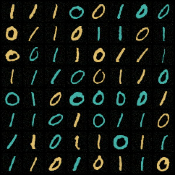
The colored MNIST experiment in Section 6.3 follows the method for composing diffusion models introduced in Section 5.3. The three base diffusion models were trained on colored MNIST digits generated from the original MNIST dataset. These colored digits were created by mapping MNIST images from their grayscale representation to either the red or green channel, leaving the other channels set to 0. For Figure 7 we post-processed the red and green images generated by the base models and compositions into beige and cyan respectively, which are more accessible colors for colorblind people.

Models, training details, and hyperparameters.

The base diffusion models were defined as VE SDEs [34]. Their score models were U-Net [65] networks consisting of 4 convolutional layers with 64, 128, 256, and 256 channels and 4 matching transposed convolutional layers. Time was encoded using 256-dimensional Gaussian random features [66]. The score model was trained using Adam optimizer [64] with a learning rate decreasing exponentially from 102superscript10210^{-2} to 104superscript10410^{-4}. We performed 200 training steps with batch size 32.

The first classifier Q~(y1,y2|xt)~𝑄subscript𝑦1conditionalsubscript𝑦2subscript𝑥𝑡\widetilde{Q}(y_{1},y_{2}|x_{t}) was a convolutional network consisting of 2 convolutional layers with 64 and 96 channels and three hidden layers with 512, 256 and 256 units. This classifier is time-dependent and used 128-dimensional Gaussian random features to embed the time. The output was a 3x3 matrix encoding the predicted log-probabilities. The classifier was trained on trajectories sampled from the reverse SDE of the base diffusion models using the AdaDelta optimizer [67] with a learning rate of 1.01.01.0. We performed 700 training steps with batch size 128. For the first 100 training steps the classifier was only trained on terminal samples.

The second conditional classifier Q~(y3|y1,y2,xt)~𝑄conditionalsubscript𝑦3subscript𝑦1subscript𝑦2subscript𝑥𝑡\widetilde{Q}(y_{3}|y_{1},y_{2},x_{t}) was a similar convolutional network with 2 convolutional layers with 64 channels and two hidden layers with 256 units. This classifier is conditioned both on time and on (y1,y2)subscript𝑦1subscript𝑦2(y_{1},y_{2}). The time variable was embedded used 128-dimensional Gaussian random features. The (y1,y2)subscript𝑦1subscript𝑦2(y_{1},y_{2}) variables were encoded using a 1-hot encoding scheme. The output of the classifier was the three predicted log-probabilities for y3subscript𝑦3y_{3}. Contrary to the first classifier, this one was not trained on the base diffusion models but rather on samples from the posterior p~(x|y1,y2)~𝑝conditional𝑥subscript𝑦1subscript𝑦2\widetilde{p}(x|y_{1},y_{2}). It’s loss function was:

c(ϕ)=𝔼(x^0,x^t,y^2,y^1,t)p~(x0,xt|y1,y2)p~(y1)p~(y2)p(t)[y^3=1mwy^3(x^0)logQ~ϕ(y^3|y^1,y^2,x^t)]subscript𝑐italic-ϕsubscript𝔼similar-tosubscript^𝑥0subscript^𝑥𝑡subscript^𝑦2subscript^𝑦1𝑡~𝑝subscript𝑥0conditionalsubscript𝑥𝑡subscript𝑦1subscript𝑦2~𝑝subscript𝑦1~𝑝subscript𝑦2𝑝𝑡superscriptsubscriptsubscript^𝑦31𝑚subscript𝑤subscript^𝑦3subscript^𝑥0subscript~𝑄italic-ϕconditionalsubscript^𝑦3subscript^𝑦1subscript^𝑦2subscript^𝑥𝑡\mathcal{L}_{c}(\phi)=\operatornamewithlimits{\mathbb{E}}_{(\widehat{x}_{0},\widehat{x}_{t},\widehat{y}_{2},\widehat{y}_{1},t)\sim\widetilde{p}(x_{0},x_{t}|y_{1},y_{2})\widetilde{p}(y_{1})\widetilde{p}(y_{2})p(t)}\left[\sum_{\widehat{y}_{3}=1}^{m}-w_{\widehat{y}_{3}}(\widehat{x}_{0})\log\widetilde{Q}_{\phi}(\widehat{y}_{3}|\widehat{y}_{1},\widehat{y}_{2},\widehat{x}_{t})\right] (115)

where wy^3(x^0)subscript𝑤subscript^𝑦3subscript^𝑥0w_{\widehat{y}_{3}}(\widehat{x}_{0}) is estimated using the first classifier. The classifier was trained using the AdaDelta optimizer [67] with a learning rate of 0.10.10.1. We performed 200 training steps with batch size 128.

Sampling.

Sampling from both the individual base models and the composition was done using the Predictor-Corrector sampler [34]. We performed sampling over 500 time steps to generate the samples shown in Figure 7. The samples used to train the classifier were generated using the same method.

When sampling from the composition we found that using scaling for the classifier guidance was generally necessary to achieve high-quality results. Without scaling, the norm of the gradient over the first and second classifier was too small relative to the gradient predicted by the score function, and hence did not sufficiently steer the mixture towards samples from the posterior. Experimentally, we found that scaling factor 10 for the first classifier and scaling factor 75 for the second produced high quality results.

Appendix F Additional Results

F.1 Binary Operations for MNIST Digit Generation via Diffusion Models
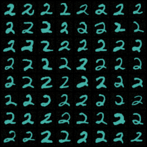
Here we present a variant of the colored digit generation experiment from Section 6.3 using 2 diffusion models. This allows us to better illustrate the harmonic mean and contrast operations on this image domain. In a similar fashion to the experiment in Section 6.3, we trained two diffusion models to generate colored MNIST digits. p1subscript𝑝1p_{1} was trained to generate red and green 0 digits and p2subscript𝑝2p_{2} was trained to generate green 0 and 1 digits. As before, we used post-processing to map green to cyan and red to beige.

Implementation details.

The diffusion models used in this experiment and their training procedure were exactly the same as in Section E.3. The sampling method used to obtain samples from the base models and their compositions was also the same. We found that scaling the classifier guidance was generally required for high-quality results, and used a scaling factor of 20 in this experiment.

The classifier was a convolutional network with 2 convolutional layers consisting of 32 and 64 channels and two hidden layers with 512 and 128 units. The classifier’s time input was embedded using 128-dimensional Gaussian random features. The output was a 2x2 matrix encoding the predicted log-probabilities Q~(y1,y2|xt)~𝑄subscript𝑦1conditionalsubscript𝑦2subscript𝑥𝑡\widetilde{Q}(y_{1},y_{2}\,|\,x_{t}). The classifier was trained on trajectories, sampled from the reverse SDE of the base diffusion models, using the AdaDelta optimizer [67] with a learning rate of 0.10.10.1 and a decay rate of 0.970.970.97. We performed 200 training steps with batch size 128. For the first 100 training steps, the classifier was only trained on terminal samples.

Results.

Figure F.1 shows samples obtained from the two trained diffusion models p1subscript𝑝1p_{1}, p2subscript𝑝2p_{2} and from the harmonic mean and contrast compositions of these models. We observe that the harmonic mean generates only cyan zero digits, because this is the only type of digit on which both p1subscript𝑝1p_{1} and p2subscript𝑝2p_{2} have high density. The contrast p1\circlerighthalfblackp2subscript𝑝1\circlerighthalfblacksubscript𝑝2p_{1}{\,\circlerighthalfblack\,}p_{2} generates beige zero digits from p1subscript𝑝1p_{1}. However, unlike p1subscript𝑝1p_{1}, it does not generate cyan zero digits, as p2subscript𝑝2p_{2} has high density there. The story is similar for p1\circlelefthalfblackp2subscript𝑝1\circlelefthalfblacksubscript𝑝2p_{1}{\,\circlelefthalfblack\,}p_{2}, which generates cyan one digits from p2subscript𝑝2p_{2}, but not zero digits due to p1subscript𝑝1p_{1} having high density over those.

Refer to caption
(a) p1subscript𝑝1p_{1}
Refer to caption
(b) p2subscript𝑝2p_{2}
Refer to caption
(c) p1p2tensor-productsubscript𝑝1subscript𝑝2p_{1}\otimes p_{2}
Refer to caption
(d) p1\circlerighthalfblackp2subscript𝑝1\circlerighthalfblacksubscript𝑝2p_{1}{\,\circlerighthalfblack\,}p_{2}
Refer to caption
(e) p1\circlelefthalfblackp2subscript𝑝1\circlelefthalfblacksubscript𝑝2p_{1}{\,\circlelefthalfblack\,}p_{2}
Figure F.1: Diffusion model composition on colored MNIST. (a,b) samples from base diffusion models. (c-e) samples from the resulting harmonic mean and contrast compositions.

F.2 MNIST Subset Generation via Diffusion Models
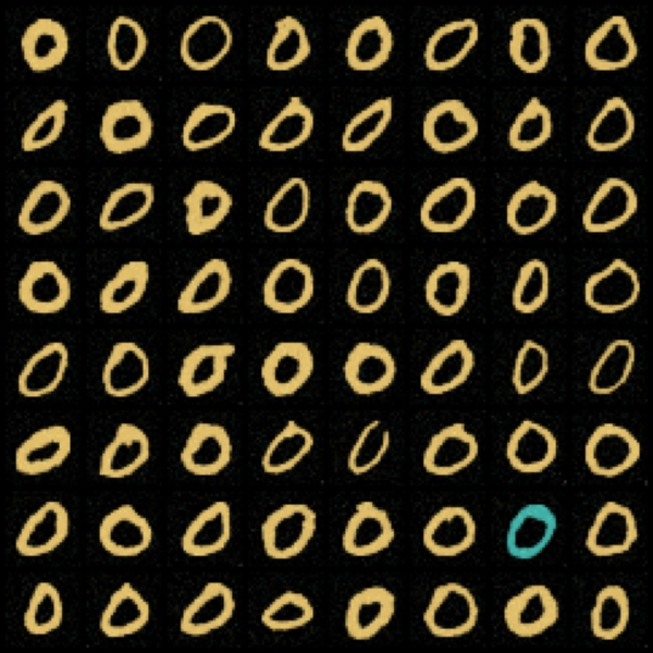
We report in this section on additional results for composing diffusion models on the standard MNIST dataset. We trained two diffusion models: p{0,,5}subscript𝑝05p_{\{0,\dots,5\}} was trained to generate MNIST digits 0 through 5, and p{4,,9}subscript𝑝49p_{\{4,\dots,9\}} to generate MNIST digits 4 through 9. The training procedure and models used in this experiment were the same as in Section F.1.
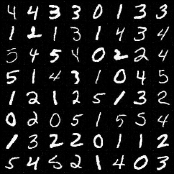
Refer to caption
(a) p{0,,5}subscript𝑝05p_{\{0,\dots,5\}}
Refer to caption
(b) p{4,,9}subscript𝑝49p_{\{4,\dots,9\}}
Refer to caption
(c) p{0,,5}p{4,,9}tensor-productsubscript𝑝05subscript𝑝49p_{\{0,\dots,5\}}\otimes p_{\{4,\dots,9\}}
Refer to caption
(d) p{0,,5}\circlerighthalfblackp{4,,9}subscript𝑝05\circlerighthalfblacksubscript𝑝49p_{\{0,\dots,5\}}{\,\circlerighthalfblack\,}p_{\{4,\dots,9\}}
Refer to caption
(e) p{0,,5}\circlelefthalfblackp{4,,9}subscript𝑝05\circlelefthalfblacksubscript𝑝49p_{\{0,\dots,5\}}{\,\circlelefthalfblack\,}p_{\{4,\dots,9\}}
Figure F.2: Diffusion model composition on MNIST. (a,b) samples from base diffusion models. (c-e) samples from the resulting harmonic mean and contrast compositions.

Figure F.2 shows samples obtained from the two diffusion models, from the harmonic mean, and from the contrast compositions of these models. We observe that the harmonic mean correctly generates mostly images on which both diffusion models’ sampling distributions have high probability, i.e. digits 4 and 5. For the contrasts we see that in both cases digits are generated that have high probability under one model but low probability under the other. We observe some errors, namely some 9’s being generated by the harmonic mean and some 4’s being generated by the contrast p{0,,5}\circlelefthalfblackp{4,,9}subscript𝑝05\circlelefthalfblacksubscript𝑝49p_{\{0,\dots,5\}}{\,\circlelefthalfblack\,}p_{\{4,\dots,9\}}. This is likely because 4 and 9 are visually similar, causing the guiding classifier to misclassify them, and generate them under the wrong composition.

We also present binary operations between three distributions. In Figure F.3 and F.4, p0subscript𝑝0p_{0} models even digits, p1subscript𝑝1p_{1} models odd digits, and p2subscript𝑝2p_{2} models digits that are divisible by 333. We color digits {0,6}06\{0,6\} purple, {3,9}39\{3,9\} blue, {4,8}48\{4,8\} orange, and {1,5,7}157\{1,5,7\} beige. In Figure F.3, harmonic mean of p0subscript𝑝0p_{0} and p2subscript𝑝2p_{2} generates the digit 00 and 666, whereas the contrast of p0subscript𝑝0p_{0} with p2subscript𝑝2p_{2} shows even digits non-divisible by 333 (p0\circlerighthalfblackp2={4,8}subscript𝑝0\circlerighthalfblacksubscript𝑝248p_{0}{\,\circlerighthalfblack\,}p_{2}=\{4,8\}), and odd numbers that are divisible by 333 (p0\circlelefthalfblackp2={3,9}subscript𝑝0\circlelefthalfblacksubscript𝑝239p_{0}{\,\circlelefthalfblack\,}p_{2}=\{3,9\}). We observe that the samples from p0p2tensor-productsubscript𝑝0subscript𝑝2p_{0}\otimes p_{2} inherit artifacts from the base generator for p2subscript𝑝2p_{2} (the thin digit 00), which shows the impact that the base models have on the composite distribution. In Figure F.4 we present similar results between odd digits ({5,3,5,7,9}53579\{5,3,5,7,9\}. We noticed that samples from both p1\circlerighthalfblackp2subscript𝑝1\circlerighthalfblacksubscript𝑝2p_{1}{\,\circlerighthalfblack\,}p_{2} and p1\circlelefthalfblackp2subscript𝑝1\circlelefthalfblacksubscript𝑝2p_{1}{\,\circlelefthalfblack\,}p_{2} includes a small number of the digit 333.

Refer to caption
(a) p0subscript𝑝0p_{0}: Even Digits
Refer to caption
(b) p2subscript𝑝2p_{2}: {0,3,6,9}0369\{0,3,6,9\}
Refer to caption
(c) p0p2tensor-productsubscript𝑝0subscript𝑝2p_{0}\otimes p_{2}
Refer to caption
(d) p0\circlerighthalfblackp2subscript𝑝0\circlerighthalfblacksubscript𝑝2p_{0}{\,\circlerighthalfblack\,}p_{2}
Refer to caption
(e) p0\circlelefthalfblackp2subscript𝑝0\circlelefthalfblacksubscript𝑝2p_{0}{\,\circlelefthalfblack\,}p_{2}
Figure F.3: Composing even digits and multiples of three. (a,b) samples from base diffusion models. (c-e) samples from the resulting harmonic mean and contrast compositions.
Refer to caption
(a) p1subscript𝑝1p_{1}: Odd Digits
Refer to caption
(b) p2subscript𝑝2p_{2}: {0,3,6,9}0369\{0,3,6,9\}
Refer to caption
(c) p1p2tensor-productsubscript𝑝1subscript𝑝2p_{1}\otimes p_{2}
Refer to caption
(d) p1\circlerighthalfblackp2subscript𝑝1\circlerighthalfblacksubscript𝑝2p_{1}{\,\circlerighthalfblack\,}p_{2}
Refer to caption
(e) p1\circlelefthalfblackp2subscript𝑝1\circlelefthalfblacksubscript𝑝2p_{1}{\,\circlelefthalfblack\,}p_{2}
Figure F.4: Composing odd digits and multiples of three. (a,b) samples from base diffusion models. (c-e) samples from the resulting harmonic mean and contrast compositions.

F.3 Chaining: Sequential Composition of Multiple Distributions

We present results on chaining binary composition operations sequentially on a custom colored MNIST dataset.

Setup.

We start with three base generative models that are trained to generate p1subscript𝑝1p_{1}, p2subscript𝑝2p_{2} and p3subscript𝑝3p_{3} in Figure F.5. Specifically, p1subscript𝑝1p_{1} is a uniform distribution over digits {0,1,2,3,4,5}012345\{0,1,2,3,4,5\}, p2subscript𝑝2p_{2} is a uniform distribution over even digits {0,2,4,6,8}02468\{0,2,4,6,8\}, and p3subscript𝑝3p_{3} is a uniform distribution over digits divisible by 333: {0,3,6,9}0369\{0,3,6,9\}. Note that we use a different color for each digit consistent across p1,p2,p3subscript𝑝1subscript𝑝2subscript𝑝3p_{1},p_{2},p_{3}. Our goal is to produce combinations of chained binary operations involving all three distributions, where two of them were combined first, then in a second step, combined with the third distribution through either harmonic mean tensor-product\otimes or contrast \circlerighthalfblack\circlerighthalfblack{\,\circlerighthalfblack\,}.

Binary Classifier Training.

Consider, for example, the operation (p1p2)\circlerighthalfblackp3tensor-productsubscript𝑝1subscript𝑝2\circlerighthalfblacksubscript𝑝3(p_{1}\otimes p_{2}){\,\circlerighthalfblack\,}p_{3}. We use the same classifier training procedure for p1subscript𝑝1p_{1} versus p2subscript𝑝2p_{2}, as well as the composite model (p1p2)tensor-productsubscript𝑝1subscript𝑝2(p_{1}\otimes p_{2}) versus p3subscript𝑝3p_{3}, except that in the later case we sample from composite model as a whole. Our classifier training simultaneously optimizes the terminal classifier and the intermediate state classifier.

Implementation Detains.

We adapted diffusion model training code for the base distributions from [33]. Our diffusion model used a UNet backbone with four latent layers on both the contracting and the expansive path. The contracting channel dimensions were [64,128,256,256]64128256256[64,128,256,256] with the kernel size 333, and strides [1,2,2,2]1222[1,2,2,2]. The time embedding used a mixture of 128128128 sine and cosine feature pairs, with a total of 256256256 dimensions. These features were passed through a sigmoid activation and then expanded using a different linear head for each layer. The activations were then added to the 2D feature maps at each layer channel-wise. We used a fixed learning rate of 0.010.010.01 with Adam optimizer [64].

We adapted the classifier training code from the MNIST example in Pytorch [68]. Our binary classifier has two latent layers with channel dimensions [32,64]3264[32,64], stride 111 and kernel width of 333. We use dropout on both layers: p1=25%,p2=50%formulae-sequencesubscript𝑝1percent25subscript𝑝2percent50p_{1}=25\%,p_{2}=50\%. We train the network for 200 epochs on data sampled online in batches of 256256256 from each source model, and treat the composite model in the second step the same way. We use the Adadelta [67] optimizer with the default setting of learning rate 1.01.01.0.

Sampling.

We generate samples according to Sec 5.3 and multiply the gradient by α=20𝛼20\alpha=20.

Results.

Row 3 from Figure F.5 contains mostly zeros with a few exceptions. This is in agreement with harmonic mean being symmetric. In p1(p2p3)tensor-productsubscript𝑝1tensor-productsubscript𝑝2subscript𝑝3p_{1}\otimes(p_{2}\otimes p_{3}), digits that are outside of the intersection still appear with thin strokes.
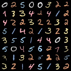
Refer to caption
(a) p1{05}subscript𝑝105p_{1}\{0-5\}
Refer to caption
(b) p2{0,2,4,6,8}subscript𝑝202468p_{2}\{0,2,4,6,8\}
Refer to caption
(c) p3{0,3,6,9}subscript𝑝30369p_{3}\{0,3,6,9\}
Refer to caption
(d) p1p2tensor-productsubscript𝑝1subscript𝑝2p_{1}\otimes p_{2}
Refer to caption
(e) p2p3tensor-productsubscript𝑝2subscript𝑝3p_{2}\otimes p_{3}
Refer to caption
(f) p1p3tensor-productsubscript𝑝1subscript𝑝3p_{1}\otimes p_{3}
Refer to caption
(g) p1\circlerighthalfblackp2subscript𝑝1\circlerighthalfblacksubscript𝑝2p_{1}{\,\circlerighthalfblack\,}p_{2}
Refer to caption
(h) p2\circlerighthalfblackp3subscript𝑝2\circlerighthalfblacksubscript𝑝3p_{2}{\,\circlerighthalfblack\,}p_{3}
Refer to caption
(i) p1\circlelefthalfblackp3subscript𝑝1\circlelefthalfblacksubscript𝑝3p_{1}{\,\circlelefthalfblack\,}p_{3}
Refer to caption
(j) p1\circlelefthalfblackp2subscript𝑝1\circlelefthalfblacksubscript𝑝2p_{1}{\,\circlelefthalfblack\,}p_{2}
Refer to caption
(k) p2\circlelefthalfblackp3subscript𝑝2\circlelefthalfblacksubscript𝑝3p_{2}{\,\circlelefthalfblack\,}p_{3}
Refer to caption
(l) p1\circlerighthalfblackp3subscript𝑝1\circlerighthalfblacksubscript𝑝3p_{1}{\,\circlerighthalfblack\,}p_{3}
Refer to caption
p1(p2p3)tensor-productsubscript𝑝1tensor-productsubscript𝑝2subscript𝑝3p_{1}\otimes(p_{2}\otimes p_{3})
Refer to caption
p2(p1p3)tensor-productsubscript𝑝2tensor-productsubscript𝑝1subscript𝑝3p_{2}\otimes(p_{1}\otimes p_{3})
Refer to caption
p3(p1p2)tensor-productsubscript𝑝3tensor-productsubscript𝑝1subscript𝑝2p_{3}\otimes(p_{1}\otimes p_{2})
Refer to caption
p1\circlerighthalfblack(p2\circlerighthalfblackp3)subscript𝑝1\circlerighthalfblacksubscript𝑝2\circlerighthalfblacksubscript𝑝3p_{1}{\,\circlerighthalfblack\,}(p_{2}{\,\circlerighthalfblack\,}p_{3})
Refer to caption
p1\circlerighthalfblack(p2p3)subscript𝑝1\circlerighthalfblacktensor-productsubscript𝑝2subscript𝑝3p_{1}{\,\circlerighthalfblack\,}(p_{2}\otimes p_{3})
Refer to caption
p1\circlerighthalfblack(p2\circlelefthalfblackp3)subscript𝑝1\circlerighthalfblacksubscript𝑝2\circlelefthalfblacksubscript𝑝3p_{1}{\,\circlerighthalfblack\,}(p_{2}{\,\circlelefthalfblack\,}p_{3})
Refer to caption
p2\circlerighthalfblack(p1\circlerighthalfblackp3)subscript𝑝2\circlerighthalfblacksubscript𝑝1\circlerighthalfblacksubscript𝑝3p_{2}{\,\circlerighthalfblack\,}(p_{1}{\,\circlerighthalfblack\,}p_{3})
Refer to caption
p2\circlerighthalfblack(p1p3)subscript𝑝2\circlerighthalfblacktensor-productsubscript𝑝1subscript𝑝3p_{2}{\,\circlerighthalfblack\,}(p_{1}\otimes p_{3})
Refer to caption
p2\circlerighthalfblack(p1\circlelefthalfblackp3)subscript𝑝2\circlerighthalfblacksubscript𝑝1\circlelefthalfblacksubscript𝑝3p_{2}{\,\circlerighthalfblack\,}(p_{1}{\,\circlelefthalfblack\,}p_{3})
Refer to caption
p3\circlerighthalfblack(p1\circlerighthalfblackp2)subscript𝑝3\circlerighthalfblacksubscript𝑝1\circlerighthalfblacksubscript𝑝2p_{3}{\,\circlerighthalfblack\,}(p_{1}{\,\circlerighthalfblack\,}p_{2})
Refer to caption
p3\circlerighthalfblack(p1p2)subscript𝑝3\circlerighthalfblacktensor-productsubscript𝑝1subscript𝑝2p_{3}{\,\circlerighthalfblack\,}(p_{1}\otimes p_{2})
Refer to caption
p3\circlerighthalfblack(p1\circlelefthalfblackp2)subscript𝑝3\circlerighthalfblacksubscript𝑝1\circlelefthalfblacksubscript𝑝2p_{3}{\,\circlerighthalfblack\,}(p_{1}{\,\circlelefthalfblack\,}p_{2})
Refer to caption
p1(p1\circlerighthalfblackp3)tensor-productsubscript𝑝1subscript𝑝1\circlerighthalfblacksubscript𝑝3p_{1}\otimes(p_{1}{\,\circlerighthalfblack\,}p_{3})
Refer to caption
p1(p2\circlelefthalfblackp3)tensor-productsubscript𝑝1subscript𝑝2\circlelefthalfblacksubscript𝑝3p_{1}\otimes(p_{2}{\,\circlelefthalfblack\,}p_{3})
Refer to caption
p2(p1\circlerighthalfblackp3)tensor-productsubscript𝑝2subscript𝑝1\circlerighthalfblacksubscript𝑝3p_{2}\otimes(p_{1}{\,\circlerighthalfblack\,}p_{3})
Refer to caption
p2(p1\circlelefthalfblackp3)tensor-productsubscript𝑝2subscript𝑝1\circlelefthalfblacksubscript𝑝3p_{2}\otimes(p_{1}{\,\circlelefthalfblack\,}p_{3})
Refer to caption
p3(p1\circlerighthalfblackp2)tensor-productsubscript𝑝3subscript𝑝1\circlerighthalfblacksubscript𝑝2p_{3}\otimes(p_{1}{\,\circlerighthalfblack\,}p_{2})
Refer to caption
p3(p1\circlelefthalfblackp2)tensor-productsubscript𝑝3subscript𝑝1\circlelefthalfblacksubscript𝑝2p_{3}\otimes(p_{1}{\,\circlelefthalfblack\,}p_{2})
Refer to caption
p1(p2\circlerighthalfblackp3)tensor-productsubscript𝑝1subscript𝑝2\circlerighthalfblacksubscript𝑝3p_{1}\otimes(p_{2}{\,\circlerighthalfblack\,}p_{3})
Refer to caption
p1\circlelefthalfblack(p2p3)subscript𝑝1\circlelefthalfblacktensor-productsubscript𝑝2subscript𝑝3p_{1}{\,\circlelefthalfblack\,}(p_{2}\otimes p_{3})
Refer to caption
p2\circlelefthalfblack(p1p3)subscript𝑝2\circlelefthalfblacktensor-productsubscript𝑝1subscript𝑝3p_{2}{\,\circlelefthalfblack\,}(p_{1}\otimes p_{3})
Figure F.5: Chaining Binary Operations. (a-c) Samples from 3 pre-trained diffusion models. (d-l) Samples from binary compositions. (row 3) The harmonic mean between all three. (row 4 and beyond) various ways to chain the operations. Parentheses indicate the order of composition.

F.4 Classifier Learning Curves and Training Time
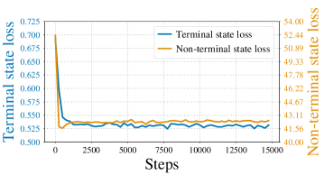
Refer to caption
Refer to caption
Figure F.6: Training curves of the classifier Q~ϕ(y1,y2|)subscript~𝑄italic-ϕsubscript𝑦1conditionalsubscript𝑦2\widetilde{Q}_{\phi}(y_{1},y_{2}|\cdot) in GFlowNet 2D grid domain. The experimental setup corresponds to Section 6.1 and Figure 3 (top row). Left: Terminal state loss and non-terminal state loss (as defined in Algorithm 1) as functions of the number of training steps. Right: L1subscript𝐿1L_{1} distance between learned distributions (compositions obtained through classifier-based mixture and guidance) and ground-truth composition distributions as the function of the number of training steps. L1(p,q)=x𝒳|p(x)q(x)|subscript𝐿1𝑝𝑞subscript𝑥𝒳𝑝𝑥𝑞𝑥L_{1}(p,q)=\sum_{x\in\mathcal{X}}|p(x)-q(x)|.
Refer to caption
Figure F.7: Training curves of the classifier Q~ϕ(y1,y2|)subscript~𝑄italic-ϕsubscript𝑦1conditionalsubscript𝑦2\widetilde{Q}_{\phi}(y_{1},y_{2}|\cdot) in GFlowNet molecule generation domain. The experimental setup corresponds to Section 6.2 and Figure 4 (a-c). The curves show terminal state loss and non-terminal state loss (as defined in Algorithm 1) as functions of the number of training steps.
Refer to caption
Figure F.8: Training curves of the classifier Q~ϕ(y1,y2|)subscript~𝑄italic-ϕsubscript𝑦1conditionalsubscript𝑦2\widetilde{Q}_{\phi}(y_{1},y_{2}|\cdot) in diffusion MNIST image generation domain. The experimental setup corresponds to Section F.1 and Figure F.1. The curves show terminal state loss and non-terminal state loss (as defined in equations (29), (31)) as functions of the number of training steps. The non-terminal loss optimization begins after the first 100100100 training steps (shown by the black dashed line).
Figure F.9: Summary of base GFlowNet and classifier training time in molecule generation domain. The experimental setup corresponds to Section 6.2 & Figure 4 (a-c). All models were trained with a single GeForce RTX 2080 Ti GPU.
Base GFlowNet training steps 20 0002000020\,000
Base GFlowNet batch size 646464
Base GFlowNet training elapsed real time 6h 47m 11s
Classifier training steps 15 0001500015\,000
Classifier batch size 8 trajectories per base model
(all states used)
Classifier training total elapsed real time 9h 2m 19s
Classifier training data generation time 6h 35m 58s (73%percent7373\%)
Figure F.10: Summary of base diffusion and classifier training time in MNIST image generation domain. The experimental setup corresponds to Section F.1 & Figure F.1 in the main paper. All models were trained with a single Tesla V100 GPU.
Base diffusion training steps 200200200
Base diffusion batch size 323232
Base diffusion training elapsed real time 10m 6s
Classifier training steps 200200200
Classifier batch size 128 trajectories per base model
(35 time-steps per trajectory)
Classifier training total elapsed real time 30m 12s
Classifier training data generation time 29m 22s (97%percent9797\%)

We empirically evaluated classifier training time and learning curves. The results are shown in Figures F.6, F.8, F.8 and Tables F.10, F.10.

Figures F.6, F.8, F.8 show the cross-entropy loss of the classifier for terminal (21) and non-terminal states (23) as a function of the number of training steps for the GFlowNet 2D grid domain, the molecular generation domain, and the Colored MNIST digits domain respectively. They show that the loss drops quickly but remains above 0. Figure F.6 further shows the distances between the learned compositions and the ground truth distributions as a function of the number of training steps of the classifier. For all compositions, as the classifier training progresses, the distance to the ground truth distribution decreases. Compared to the distance at initialization we observe almost an order of magnitude distance reduction by the end of the training.

The runtime of classifier training is shown in Tables F.10 and F.10. We report the total runtime, as well as separate measurements for the time spent sampling trajectories and training the classifier. The classifier training time is comparable to the base generative model training time. However, most of the classifier training time (more than 70%, or even 90%) was spent on sampling trajectories from base generative models. Our implementation of the training could be improved in this regard, e.g. by sampling a smaller set of trajectories once and re-using trajectories for training and by reducing the number of training steps (the loss curves in Figures F.6, F.8, F.8 show that classification losses plateau quickly).

F.5 Analysis of Sample Diversity of Base GFlowNets in Molecule Generation Domain

In order to assess the effect of the reward exponent β𝛽\beta on mode coverage and sample diversity, we evaluated samples generated from GFlowNets pre-trained with different values of β𝛽\beta. The results are in Tables F.12 and F.12. The details of the evaluation and the reported metrics are described in the table captions. As expected, larger reward exponents shift the learned distributions towards high-scoring molecules (the total number of molecules with scores above the threshold increases). For ‘SA’ and ‘QED’ models we don’t observe negative effects of large β𝛽\beta on sample diversity and mode coverage: the average pairwise similarity of top 1 00010001\,000 molecules doesn’t grow as β𝛽\beta increases and the ratio of Tanimoto-separated modes remains high. For ‘SEH’ models we observe a gradual increase in the average pairwise similarity of top 1 00010001\,000 molecules and a gradual decrease in the ratio of Tanimoto-separated modes. However, the total number of separated modes grows as β𝛽\beta increases, which indicates that larger reward exponents do not lead to mode dropping.

Figure F.11: Average pairwise similarity [36] of molecules generated by GFlowNets trained on ’SEH’, ’SA’, ’QED’ rewards at different values of β𝛽\beta. For each combination (reward, β𝛽\beta) a GFlowNet was trained with the corresponding reward R(x)β𝑅superscript𝑥𝛽R(x)^{\beta}. Then, 5 00050005\,000 molecules were generated. The numbers in the table reflect the average pairwise Tanimoto similarity of top 1 00010001\,000 molecules (selected according to the target reward function).
SEH SA QED
β=1𝛽1\beta=1 0.5270.5270.527 0.5390.5390.539 0.4800.4800.480
β=4𝛽4\beta=4 0.5290.5290.529 0.5270.5270.527 0.4640.4640.464
β=10𝛽10\beta=10 0.5350.5350.535 0.5000.5000.500 0.4380.4380.438
β=16𝛽16\beta=16 0.5480.5480.548 0.4650.4650.465 0.4220.4220.422
β=32𝛽32\beta=32 0.5850.5850.585 0.4110.4110.411 0.3980.3980.398
β=96𝛽96\beta=96 0.6180.6180.618 0.3580.3580.358 0.4040.4040.404
Figure F.12: Number of Tanimoto-separated modes found above reward threshold. For each combination (reward, β𝛽\beta) a GFlowNet was trained with the corresponding reward R(x)β𝑅superscript𝑥𝛽R(x)^{\beta}, and then 5 00050005\,000 molecules were generated. Cell format is "A/B𝐴𝐵A/B", where A𝐴A is the number of Tanimoto-separated modes found above the reward threshold, and B𝐵B is the total number of generated molecules above the threshold. Analogously to Figure 14 in [36], we consider having found a new mode representative when a new molecule has Tanimoto similarity smaller than 0.70.70.7 to every previously found mode’s representative molecule. Reward thresholds (in [0,1]01[0,1], normalized values) are ’SEH’: 0.8750.8750.875, ’SA’: 0.750.750.75, ’QED’: 0.750.750.75. Note that the normalized threshold of 0.8750.8750.875 for ’SEH’ corresponds to the unnormalized threshold of 777 used in [36].
SEH SA QED
β=1𝛽1\beta=1 15/ 1715 17\hbox to20.00006pt{\hfill 15}\,/\,\hbox to20.00006pt{\hfill 17} 37/ 3737 37\hbox to20.00006pt{\hfill 37}\,/\,\hbox to20.00006pt{\hfill 37} 0/ 00 0\hbox to20.00006pt{\hfill 0}\,/\,\hbox to20.00006pt{\hfill 0}
β=4𝛽4\beta=4 12/ 1712 17\hbox to20.00006pt{\hfill 12}\,/\,\hbox to20.00006pt{\hfill 17} 82/ 8282 82\hbox to20.00006pt{\hfill 82}\,/\,\hbox to20.00006pt{\hfill 82} 0/ 00 0\hbox to20.00006pt{\hfill 0}\,/\,\hbox to20.00006pt{\hfill 0}
β=10𝛽10\beta=10 85/ 10985 109\hbox to20.00006pt{\hfill 85}\,/\,\hbox to20.00006pt{\hfill 109} 332/ 337332 337\hbox to20.00006pt{\hfill 332}\,/\,\hbox to20.00006pt{\hfill 337} 18/ 1818 18\hbox to20.00006pt{\hfill 18}\,/\,\hbox to20.00006pt{\hfill 18}
β=16𝛽16\beta=16 190/ 280190 280\hbox to20.00006pt{\hfill 190}\,/\,\hbox to20.00006pt{\hfill 280} 886/ 910886 910\hbox to20.00006pt{\hfill 886}\,/\,\hbox to20.00006pt{\hfill 910} 253/ 253253 253\hbox to20.00006pt{\hfill 253}\,/\,\hbox to20.00006pt{\hfill 253}
β=32𝛽32\beta=32 992/ 1821992 1821\hbox to20.00006pt{\hfill 992}\,/\,\hbox to20.00006pt{\hfill 1821} 2859/ 30802859 3080\hbox to20.00006pt{\hfill 2859}\,/\,\hbox to20.00006pt{\hfill 3080} 3067/ 31243067 3124\hbox to20.00006pt{\hfill 3067}\,/\,\hbox to20.00006pt{\hfill 3124}
β=96𝛽96\beta=96 1619/ 46091619 4609\hbox to20.00006pt{\hfill 1619}\,/\,\hbox to20.00006pt{\hfill 4609} 4268/ 49834268 4983\hbox to20.00006pt{\hfill 4268}\,/\,\hbox to20.00006pt{\hfill 4983} 4470/ 49804470 4980\hbox to20.00006pt{\hfill 4470}\,/\,\hbox to20.00006pt{\hfill 4980}
Table F.1: Estimated pairwise earthmover’s distances between distributions shown in Table 6.
y=SEH y=SA y=QED y=SEH,SA y=SEH,QED y=SA,QED y=SEH,SA,QED y=SEH × 3absent3\times\;3 y=SA × 3absent3\times\;3 y=QED × 3absent3\times\;3
y=SEH 0 4.42 5.77 3.39 4.20 4.88 4.10 2.46 4.44 5.73
y=SA 4.42 0 5.88 3.26 5.15 4.59 4.20 4.39 2.55 5.89
y=QED 5.77 5.88 0 5.40 4.02 3.85 4.20 5.80 5.90 3.20
y=SEH,SA 3.39 3.26 5.40 0 4.25 4.19 3.68 3.39 3.30 5.39
y=SEH,QED 4.20 5.15 4.02 4.25 0 3.80 3.67 4.22 5.19 4.00
y=SA,QED 4.88 4.59 3.85 4.19 3.80 0 3.65 4.91 4.59 3.87
y=SEH,SA,QED 4.10 4.20 4.20 3.68 3.67 3.65 0 4.12 4.23 4.20
y=SEH × 3absent3\times\;3 2.46 4.39 5.80 3.39 4.22 4.91 4.12 0 4.43 5.73
y=SA × 3absent3\times\;3 4.44 2.55 5.90 3.30 5.19 4.59 4.23 4.43 0 5.90
y=QED × 3absent3\times\;3 5.73 5.89 3.20 5.39 4.00 3.87 4.20 5.73 5.90 0