Adversarial Examples Might be Avoidable: The Role of Data Concentration in Adversarial Robustness

Abstract

The susceptibility of modern machine learning classifiers to adversarial examples has motivated theoretical results suggesting that these might be unavoidable. However, these results can be too general to be applicable to natural data distributions. Indeed, humans are quite robust for tasks involving vision. This apparent conflict motivates a deeper dive into the question: Are adversarial examples truly unavoidable? In this work, we theoretically demonstrate that a key property of the data distribution – concentration on small-volume subsets of the input space – determines whether a robust classifier exists. We further demonstrate that, for a data distribution concentrated on a union of low-dimensional linear subspaces, exploiting data structure naturally leads to classifiers that enjoy good robustness guarantees, improving upon methods for provable certification in certain regimes.

1 Introduction, Motivation and Contributions

Research in adversarial learning has shown that traditional neural network based classification models are prone to anomalous behaviour when their inputs are modified by tiny, human-imperceptible perturbations. Such perturbations, called adversarial examples, lead to a large degradation in the accuracy of classifiers [50]. This behavior is problematic when such classification models are deployed in security sensitive applications. Accordingly, researchers have and continue to come up with defenses against such adversarial attacks for neural networks.

Such defenses [45, 54, 39, 21] modify the training algorithm, alter the network weights, or employ preprocessing to obtain classifiers that have improved empirical performance against adversarially corrupted inputs. However, many of these defenses have been later broken by new adaptive attacks [1, 7]. This motivated recent impossibility results for adversarial defenses, which aim to show that all defenses admit adversarial examples. While initially such results were shown for specially parameterized data distributions [17], they were subsequently expanded to cover general data distributions on the unit sphere and the unit cube [44], as well as for distributions over more general manifolds [11].

On the other hand, we humans are an example of a classifier capable of very good (albeit imperfect [16]) robust accuracy against $\ell_{2}$-bounded attacks for natural image classification. Even more, a large body of recent work has constructed certified defenses [10, 57, 9, 28, 19, 49] which obtain non-trivial performance guarantees under adversarially perturbed inputs for common datasets like MNIST, CIFAR-10 and ImageNet. This apparent contention between impossibility results and the existence of robust classifiers for natural datasets indicates that the bigger picture is more nuanced, and motivates a closer look at the impossibility results for adversarial examples.

Our first contribution is to show that these results can be circumvented by data distributions whose mass concentrates on small regions of the input space. This naturally leads to the question of whether such a construction is necessary for adversarial robustness. We answer this question in the affirmative, formally proving that a successful defense exists only when the data distribution concentrates on an exponentially small volume of the input space. At the same time, this suggests that exploiting the inherent structure in the data is critical for obtaining classifiers with broader robustness guarantees.

Surprisingly, almost all certified defenses do not exploit any structural aspects of the data distribution like concentration or low-dimensionality. Motivated by our theoretical findings, we study the special case of data distributions concentrated near a union of low-dimensional linear subspaces, to create a certified defense for perturbations that go beyond traditional $\ell_{p}$-norm bounds. We find that simply exploiting the low-dimensional data structure leads to a natural classification algorithm for which we can derive norm-independent polyhedral certificates. We show that our method can certify accurate predictions under adversarial examples with an $\ell_{p}$ norm larger than what can be certified by applying existing, off-the-shelf methods like randomized smoothing [10]. Thus, we demonstrate the importance of data structure in both the theory and practice of certified adversarial robustness.

More precisely, we make the following main contributions in this work:

1. We formalize a notion of $(\epsilon,\delta)$-concentration of a probability distribution $q$ in Section 2, which states that $q$ assigns at least $1-\delta$ mass to a subset of the ambient space having volume $O(\exp{(-\epsilon)})$. We show that $(\epsilon,\delta)$-concentration of $q$ is a necessary condition for the existence of any classifier obtaining at most $\delta$ error over $q$, under perturbations of size $\epsilon$.

2. We find that $(\epsilon,\delta)$-concentration is too general to be a sufficient condition for the existence of a robust classifier, and we follow up with a stronger notion of concentration in Section 3 which is sufficient for the existence of robust classifiers. Following this stronger notion, we construct an example of a strongly-concentrated distribution, which circumvents existing impossibility results on the existence of robust classifiers.

3. We then consider a data distribution $q$ concentrated on a union of low-dimensional linear subspaces in Section 4. We construct a classifier for $q$ that is robust to perturbations following threat models more general than $\ell_{p}$. Our analysis results in polyhedral certified regions whose faces and extreme rays are described by selected points in the training data.

4. We perform empirical evaluations on MNIST in Section 5, demonstrating that our certificates are complementary to existing off-the-shelf approaches like Randomized Smoothing (RS), in the sense that both methods have different strengths. In particular, we demonstrate a region of adversarial perturbations where our method is certifiably robust, but RS is not. We then combine our method with RS to obtain certificates that enjoy the best of both worlds.

2 Existence of Robust Classifier Implies Concentration

We will consider a classification problem over $\mathcal{X}\times\mathcal{Y}$ defined by the data distribution $p$ such that $\mathcal{X}$ is bounded and $\mathcal{Y}=\{1,2,\ldots,K\}$. We let $q_{k}$ denote the conditional distribution $p_{X|Y=k}$ for class $k\in\mathcal{Y}$. We will assume that the data is normalized, i.e., $\mathcal{X}=B_{\ell_{2}}(0,1)$, and the boundary of the domain is far from the data, i.e., for any $x\sim q_{k}$, an adversarial perturbation of $\ell_{2}$ norm at most $\epsilon$ does not take $x$ outside the domain $\mathcal{X}$.

We define the robust risk of a classifier $f\colon\mathcal{X}\to\mathcal{Y}$ against an adversary making perturbations whose $\ell_{2}$ norm is bounded by $\epsilon$ as

$$R(f,\epsilon)=\Pr_{(x,y)\sim p}\left(\exists\bar{x}\in B_{\ell_{2}}(x,\epsilon)\text{ such that }f(\bar{x})\neq y\right).$$ (1)

We can now define a robust classifier in our setting.

Definition 2.1 (Robust Classifier).

A classifier $g$ is defined to be $(\epsilon,\delta)$-robust if the robust risk against perturbations with $\ell_{2}$ norm bounded by $\epsilon$ is at most $\delta$, i.e., if $R(g,\epsilon)\leq\delta$.

The goal of this section is to show that if our data distribution $p$ admits an $(\epsilon,\delta)$–robust classifier, then $p$ has to be concentrated. Intuitively, this means that $p$ assigns a “large” measure to sets of “small” volume. We define this formally now.

Definition 2.2 (Concentrated Distribution).

A probability distribution $q$ over a domain $\mathcal{X}\subseteq\mathbb{R}^{n}$ is said to be $(\epsilon,\delta)$-concentrated, if there exists a subset $S\subseteq\mathcal{X}$ such that $q(S)\geq 1-\delta$ but ${\rm Vol}(S)\leq c_{1}\exp(-c_{2}\epsilon)$ for some constants $c_{1},c_{2}>0$. Here, ${\rm Vol}$ denotes the standard Lebesgue measure on $\mathbb{R}^{n}$, and $q(S)$ denotes the probability of sampling a point in $S$ under $q$.

With the above definitions in place, we are ready to state our first main result.

Theorem 2.1.

If there exists an $(\epsilon,\delta)$-robust classifier $f$ for a data distribution $p$, then at least one of the class conditionals $q_{1},q_{2},\ldots,q_{K}$ must be $(\epsilon,\delta)$–concentrated. Further, if the classes are balanced, then all the class conditionals are $(\epsilon,K\delta)$-concentrated.

The proof utilizes the Brunn-Minkowski theorem from high-dimensional geometry, and we provide a brief sketch here, deferring the full proof to Appendix A.

Proof Sketch.

Due to the existence of a robust classifier $f$, i.e., $R(f,\epsilon)\leq\delta$, the first observation is that there must be at least one class which is classified with robust accuracy at least $1-\delta$. Say this class is $k$, and the set of all points which do not admit an $\epsilon$-adversarial example for class $k$ is $S$. Now, the second step is to show that $S$ has the same measure (under $q_{k}$) as the $\epsilon$-shrinkage (in the $\ell_{2}$ norm) of the set of all points classified as class $k$. Finally, the third step involves using the Brunn-Minkowski theorem, to show that this $\epsilon$-shrinkage has a volume $O(\exp(-n\epsilon))$, thus completing the argument. ∎

Discussion on Theorem 2.1. We pause here to understand some implications of this result.

• Firstly, recall the apparently conflicting conclusions from Section 1 between impossibility results (suggesting that robust classifiers do not exist) and the existence of robust classifiers in practice (such as that of human vision for natural data distributions). Theorem 2.1 shows that whenever a robust classifier exists, the underlying data distribution has to be concentrated. In particular, natural distributions corresponding to MNIST, CIFAR and ImageNet must therefore be concentrated. This suggests a resolution to the conflict: concentrated distributions must somehow circumvent existing impossibility results. Indeed, this is precisely what we will show in Section 3.

• Secondly, while our results are derived for the $\ell_{2}$ norm, it is not very hard to extend this reasoning to general $\ell_{p}$ norms. In other words, whenever a classifier robust to $\ell_{p}$-norm perturbations exists, the underlying data distribution must be concentrated.

• Thirdly, Theorem 2.1 has a direct implication towards classifier design. Since we now know that natural image distributions are concentrated, one should design classifiers that are tuned for small-volume regions in the input space. This might be the deeper principle behind the recent success [61] of robust classifiers adapted to $\ell_{p}$-ball like regions in the input space.

We have thus seen that data concentration is a necessary condition for the existence of a robust classifier. A natural question is whether it is also sufficient. We address this question now.

3 Strong Concentration Implies Existence of Robust Classifier

Say our distribution $p$ is such that all the class conditionals $q_{1},q_{2},\ldots,q_{k}$ are $(\epsilon,\delta)$-concentrated. Is this sufficient for the existence of a robust classifier? The answer is negative, as we have not precluded the case where all of the $q_{k}$ are concentrated over the same subset $S$ of the ambient space. In other words, it might be possible that there exists a small-volume set $S\subseteq\mathcal{X}$ such that $q_{k}(S)$ is high for all $k$. This means that whenever a data point lies in $S$, it would be hard to distinguish which class it came from. In this case, even an accurate classifier might not exist, let alone a robust classifier. To get around such issues, we define a stronger notion of concentration, as follows.

Definition 3.1 (Strongly Concentrated Distributions).

A distribution $p$ is said to be $(\epsilon,\delta,\gamma)$-strongly-concentrated if each class conditional distribution $q_{k}$ is $(\epsilon,\delta)$-concentrated (say over the set $S_{k}\subseteq\mathcal{X}$), and $q_{k}\left(\bigcup_{k^{\prime}\neq k}S_{k^{\prime}}^{+2\epsilon}\right)\leq\gamma$, where $S^{+\epsilon}$ denotes the $\epsilon$-expansion of the set $S$ in the $\ell_{2}$ norm, i.e., $S^{+\epsilon}=\{x\colon\exists\bar{x}\in S\text{ such that }\|x-\bar{x}\|_{2}\leq\epsilon\}$.

In essence, Definition 3.1 states that each of the class conditionals are concentrated on subsets of the ambient space, which do not intersect too much with one another. Hence, it is natural to expect that we would be able to construct a robust classifier by exploiting these subsets. Building upon this idea, we are able to show Theorem 3.1:

Theorem 3.1.

If the data distribution $p$ is $(\epsilon,\delta,\gamma)$-strongly-concentrated, then there exists an $(\epsilon,\delta+\gamma)$-robust classifier for $p$.

The basic observation behind this result is that if the conditional distributions $q_{k}$ had disjoint supports which were well-separated from each other, then one could obtain a robust classifier by predicting the class $k$ on the entire $\epsilon$-expansion of the set $S_{k}$ where the conditional $q_{k}$ concentrates, for all $k$. To go beyond this idealized case, we can exploit the strong concentration condition to carefully remove the intersections at the cost of at most $\gamma$ in robust accuracy. We make these arguments more precise in the full proof, deferred to Appendix B, and we pause here to note some implications for existing results.

Implications for Existing Impossibility Results. To understand how Theorem 3.1 circumvents the previous impossibility results, consider the setting from [44] where the data domain is the sphere $\mathbb{S}^{n-1}=\{x\in\mathbb{R}^{n}\colon\|x\|_{2}=1\}$, and we have a binary classification setting with class conditionals $q_{1}$ and $q_{2}$. The adversary is allowed to make bounded perturbations w.r.t. the geodesic distance. In this setting, it can be shown (see [44, Theorem 1]) that any classifier admits $\epsilon$-adversarial examples for the minority class (say class $1$), with probability at least

$$1-\alpha_{q_{1}}\beta\exp\left(-\frac{n-1}{2}\epsilon^{2}\right),$$ (2)

where $\alpha_{q_{1}}=\sup_{x\in\mathbb{S}^{n-1}}q_{1}(x)$ depends on the conditional distribution $q_{1}$, and $\beta$ is a normalizing constant that depends on the dimension $n$. Note that this result assumes little about the conditional $q_{1}$. Now, by constructing a strongly-concentrated data distribution over the domain, we will show that the

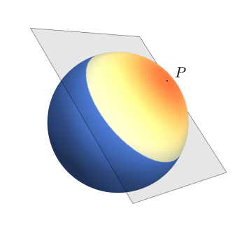
Figure 1: A plot of $q_{1}$. Redder colors denote a larger density, and the gray plane denotes the robust classifier.

lower bound in (2) becomes vacuous.

Example 3.1.

The data domain is the unit sphere $\mathbb{S}^{n-1}$ equipped with the geodesic distance $d$. The label domain is $\{1,2\}$. $P$ is an arbitrary, but fixed, point lying on $\mathbb{S}^{n-1}$. The conditional density of class $1$, i.e., $q_{1}$ is now defined as

$$q_{1}(x)=\begin{cases}\frac{1}{C}\frac{1}{\sin^{n-2}d(x,P)},&\text{ if }d(x,P)\leq 0.1\\ 0,&\text{ otherwise }\end{cases},$$

where $C=0.1$ is a normalizing constant. The conditional density of class 2 is defined to be uniform over the complement of the support of $q_{1}$, i.e. $q_{2}={\rm Unif}(\{x\in\mathbb{S}^{n-1}\colon d(x,P)>0.1\})$. Finally, the classes are balanced, i.e., $p_{Y}(1)=p_{Y}(2)=1/2$.

The data distribution constructed in Example 3.1 makes Eq. 2 vacuous, as the supremum over the density $q_{1}$ is unbounded. Additionally, the linear classifier defined by the half-space $\{x\colon\langle x,P\rangle\leq\cos(0.1)\}$ is robust (Appendix C provides a derivation of the robust risk, and further comments on generalizing this example). Example 3.1 is plotted for $n=3$ dimensions in Fig. 1.

Compatibility of Theorem 3.1 with existing Negative Results

Thus, we see that strongly concentrated distributions are able to circumvent existing impossibility results on the existence of robust classifiers. However, this does not invalidate any existing results. Firstly, measure-concentration-based results [44, 17, 11] provide non-vacuous guarantees given a sufficiently flat (not concentrated) data distribution, and hence do not contradict our results. Secondly, our results are existential and do not provide, in general, an algorithm to construct a robust classifier given a strongly-concentrated distribution. Hence, we also do not contradict the existing stream of results on the computational hardness of finding robust classifiers [5, 51, 43]. Our positive results are complementary to all such negative results, demonstrating a general class of data distributions where robust classifiers do exist.

For the reminder of this paper, we will look at a specific member of the above class of strongly concentrated data distributions and show how we can practically construct robust classifiers.

4 Adversarially Robust Classification on Union of Linear Subspaces

The union of subspaces model has been shown to be very useful in classical computer vision for a wide variety of tasks, which include clustering faces under varying illumination, image segmentation, and video segmentation [52]. Its concise mathematical description often enables the construction and theoretically analysis of algorithms that also perform well in practice. In this section, we will study robust classification on data distributions concentrated on a union of low-dimensional linear subspaces. This data structure will allow us to obtain a non-trivial, practically relevant case where we can show a provable improvement over existing methods for constructing robust classifiers in certain settings. Before delving further, we now provide a simple example (which is illustrated in Fig. 2) demonstrating how distributions concentrated about linear subspaces are concentrated precisely in the sense of Definition 3.1, and therefore allow for the existence of adversarially robust classifiers.

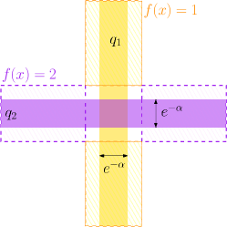
Figure 2: A plot of $q_{1}$ (orange), $q_{2}$ (violet) and the decision boundaries of $f$ (dashed).

Example 4.1.

The data domain is the ball $B_{\ell_{\infty}}(0,1)$ equipped with the $\ell_{2}$ distance. The label domain is $\{1,2\}$. Subspace $S_{1}$ is given by $S_{1}=\{x\colon x^{\top}e_{1}=0\}$, and $S_{2}$ is given by $S_{2}=\{x\colon x^{\top}e_{2}=0\}$, where $e_{1},e_{2}$ are the standard unit vectors. The conditional densities are defined as

$$q_{1} ={\rm Unif}(\{x\colon\|x\|_{\infty}\leq 1,|x^{\top}e_{1}|\leq e^{-\alpha}/2\}),\text{ and, }$$

$$q_{2} ={\rm Unif}(\{x\colon\|x\|_{\infty}\leq 1,|x^{\top}e_{2}|\leq e^{-\alpha}/2\}),$$

where $\alpha>0$ is a large constant. Finally, the classes are balanced, i.e., $p_{Y}(1)=p_{Y}(2)=1/2$. With these parameters, $q_{1},q_{2}$ are both $(\alpha,0)$-concentrated over their respective supports. Additionally, $p$ is $(\alpha,0,e^{-\alpha}/2+2\epsilon)$–strongly-concentrated. A robust classifier $f$ can be constructed following the proof of Theorem 3.1, and it obtains a robust accuracy $R(f,\epsilon)\leq e^{-\alpha}/2+2\epsilon$. See Appendix D for more details.

We will now study a specific choice of $p$ that generalizes Example 4.1 and will let us move beyond the above simple binary setting. Recall that we have a classification problem specified by a data distribution $p$ over the data domain $\mathcal{X}\times\mathcal{Y}=B(0,1)\times\{1,2,\ldots,K\}$. Firstly, the classes are balanced, i.e., $p_{Y}(k)=1/K$ for all $k\in\mathcal{Y}$. Secondly, the conditional density, i.e., $q_{k}=p_{X|Y=k}$, is concentrated on the set $S^{+\gamma}_{k}\cap\mathcal{X}$, where $S_{k}$ is a low-dimensional linear subspace, and the superscript denotes an $\gamma$-expansion, for a small $\gamma>0$.

For the purpose of building our robust classifier, we will assume access to a training dataset of $M$ clean data points $(s_{1},y_{1}),(s_{2},y_{2}),\ldots,(s_{M},y_{M})$, such that, for all $i$, the point $s_{i}$ lies exactly on one of the $K$ low-dimensional linear subspaces. We will use the notation $\mathbf{S}=[s_{1},s_{2},\ldots,s_{M}]$ for the training data matrix and $\mathbf{y}=(y_{1},y_{2},\ldots,y_{M})$ for the training labels. We will assume that $M$ is large enough that every $x\in\cup_{k}S_{k}$ can be represented as a linear combination of the columns of $\mathbf{S}$.

Now, the robust classification problem we aim to tackle is to obtain a predictor $g\colon\mathcal{X}\to\mathcal{Y}$ which obtains a low robust risk, with respect to an additive adversary $\mathcal{A}$ that we now define. For any data-point $x\sim p$, $\mathcal{A}$ will be constrained to make an additive perturbation $v$ such that ${\rm dist}_{\ell_{2}}(x+v,\cup_{i}S_{i})\leq\epsilon$. In other words, the attacked point can have $\ell_{2}$ distance at most $\epsilon$ from any of the linear subspaces $S_{1},\ldots,S_{k}$. Note that $\mathcal{A}$ is more powerful than an $\ell_{2}$-bounded adversary as the norm of the perturbation $\|v\|_{2}$ might be large, as $v$ might be parallel to a subspace.

Under such an adversary $\mathcal{A}$, given a (possibly adversarially perturbed) input $x$, it makes sense to try to recover the corresponding point $s$ lying on the union of subspaces, such that $x=s+n$, such that $\|n\|_{2}\leq\epsilon$. One way to do this is to represent $s$ as a linear combination of a small number of columns of $\mathbf{S}$, i.e., $x=\mathbf{S}c+n$. This can be formulated as an optimization problem that minimizes the cardinality of $c$, given by $\|c\|_{0}$, subject to an approximation error constraint. Since such a problem is hard because of the $\ell_{0}$ pseudo-norm, we relax this to the problem

$$\min_{c}\|c\|_{1}~{}~{}\text{s.t.}~{}~{}\|x-\mathbf{S}c\|_{2}\leq\epsilon.$$ (3)

Under a suitable choice of $\lambda$, this problem can be equivalently written as

$$\min_{c,e}\|c\|_{1}+\frac{\lambda}{2}\|e\|_{2}^{2}~{}~{}\text{s.t.}~{}~{}x=\mathbf{S}c+e,$$ (4)

for which we can obtain the dual problem given by

$$\max_{d}\langle x,d\rangle-\frac{1}{2\lambda}\|d\|_{2}^{2}~{}~{}\text{s.t.}~{}~{}\|\mathbf{S}^{\top}d\|_{\infty}\leq 1.$$ (5)

Our main observation is to leverage the stability of the set of active constraints of this dual to obtain a robust classifier. One can note that each constraint of Eq. 5 corresponds to one training data point $s_{i}$ – when the $i^{\rm th}$ constraint is active at optimality, $s_{i}$ is being used to reconstruct $x$. Intuitively, one should then somehow use the label $y_{i}$ while predicting the label for $x$. Indeed, we will show that predicting the majority label among the active $y_{i}$ leads to a robust classifier.

We will firstly obtain a geometric characterization of the problem in Eq. 5 by viewing it as the evaluation of a projection operator onto a certain convex set, illustrated in Fig. 3. Observe that for $\lambda>0$, the objective (5) is strongly convex in $d$ and the problem has a unique solution, denoted by $d^{*}_{\lambda}(x)$. It is not hard to show that this solution can be obtained by the projection operator

$$d^{*}_{\lambda}(x)=\left(\operatorname*{arg\,min}_{d}\|\lambda x-d\|_{2}~{}~{}\text{s.t. }~{}~{}\|\mathbf{S}^{\top}d\|_{\infty}\leq 1\right)={\rm Proj}_{K^{\circ}}(\lambda x),$$ (6)

where $K^{\circ}$ is the polar of the convex hull of $\pm\mathbf{S}$. Denoting $\mathbf{T}=[\mathbf{S},-\mathbf{S}]$, we can rewrite Problem (6) as $d^{*}_{\lambda}(x)=\left(\operatorname*{arg\,min}_{d}\|\lambda x-d\|_{2}\text{ sub. to }\mathbf{T}^{\top}d\leq\mathbf{1}\right)$. We now define the set of active constraints as

$$A_{\lambda}(x)=\{t_{i}\colon\langle t_{i},d^{*}_{\lambda}(x)\rangle=1\}.$$ (7)

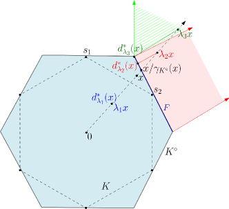
Figure 3: Geometry of the dual problem (5). See description on the left.

Geometry of the Dual (5). It is illustrated in Fig. 3, where $s_{1},s_{2}$ are two chosen data-points. The blue shaded polytope is $K^{\circ}$. At $\lambda=\lambda_{1}$, the point $\lambda_{1}x$ lies in the interior of $K^{\circ}$. Hence, $A_{\lambda}(x)$ is empty and ${\rm supp}(c^{*}(x))$ is also empty. As $\lambda$ increases, a non-empty support is obtained for the first time at $\lambda=1/\gamma_{K^{\circ}}(x)$. For all $\lambda_{2}x$ in the red shaded polyhedron, the projection $d^{*}_{\lambda_{2}}(x)={\rm Proj}_{K^{\circ}}(\lambda_{2}x)$ lies on the face $F$. As $\lambda$ increases further we reach the green polyhedron. Further increases in $\lambda$ do not change the dual solution, which will always remain at the vertex $d^{*}_{\lambda_{3}}(x)$.

Geometrically, $A_{\lambda}(x)$ identifies the face of $K^{\circ}$ which contains the projection of $\lambda x$, if $A_{\lambda}(x)$ is non-empty (otherwise, $\lambda x$ lies inside the polyhedron $K^{\circ}$). The support of the primal solution, $c^{*}(x)$, is a subset of $A_{\lambda}$, i.e.  ${\rm supp}(c^{*}(x))\subseteq A_{\lambda}(x)$. Note that whenever two points, say $x,x^{\prime}$, both lie in the same shaded polyhedron (red or green), their projections would lie on the same face of $K^{\circ}$. We now show this formally, in the main theorem of this section.

Theorem 4.1.

The set of active constraints $A_{\lambda}$ defined in (7) is robust, i.e., $A_{\lambda}(x^{\prime})=A_{\lambda}(x)$ for all $\lambda x^{\prime}\in C(x)$, where $C(x)$ is the polyhedron defined as

$$C(x)=F(x)+V(x),$$ (8)

with $F\subseteq K^{\circ}$ being a facet of the polyhedron $K^{\circ}$ that $x$ projects to, defined as

$$F(x)=\left\{d\ \left|\ \begin{aligned} &t_{i}^{\top}d=1,\forall t_{i}\in A_{\lambda}(x)\\ &t_{i}^{\top}d<1,{\rm otherwise}\end{aligned}\right.\right\},$$ (9)

and $V$ being the cone generated by the constraints active at (i.e., normal to) $F$, defined as

$$V(x)=\left\{\sum_{t_{i}\in A_{\lambda}(x)}\alpha_{i}t_{i}\colon\alpha_{i}\geq 0,\forall t_{i}\in A_{\lambda}(x)\right\}.$$ (10)

The proof of Theorem 4.1 utilizes the geometry of the problem and properties of the projection operator, and is presented in Appendix E. We can now use this result to construct a robust classifier:

Lemma 4.2.

Define the dual classifier as

$$g_{\lambda}(x)=\textsc{Aggregate}(\{y_{i}\colon t_{i}\in A_{\lambda}(x)\}),$$ (11)

where Aggregate is any deterministic mapping from a set of labels to $\mathcal{Y}$, e.g., Majority. Then, for all $x^{\prime}\in C(x)$ as defined in Theorem 4.1, $g_{\lambda}$ is certified to be robust, i.e., $g_{\lambda}(x^{\prime})=g_{\lambda}(x)$.

Implications. Having obtained a certifiably robust classifier $g$, we pause to understand some implications of the theory developed so far. We observe that the certified regions in Theorem 4.1 are not spherical, i.e., the attacker can make additive perturbations having large $\ell_{2}$ norm but still be unable to change the label predicted by $g$ (see Fig. 4). This is in contrast to the $\ell_{2}$ bounded certified regions that can be obtained by most existing work on certification schemes, and is a result of modelling data structure while constructing robust classifiers. Importantly, however, note that we do not assume that the attack is restricted to the subspace.

Connections to Classical Results. For $\epsilon=0$, Eq. 3 is known as the primal form of the Basis Pursuit problem, and has been studied under a variety of conditions on $\mathbf{S}$ in the sparse representation and subspace clustering literature [20, 12, 46, 59, 29, 24]. Given an optimal solution $c^{*}(x)$ of this basis pursuit problem, how can we accurately predict the label $y$? One ideal situation could be that all columns in the support predict the same label, i.e., $y_{i}$ is identical for all $i\in\text{supp}(c^{*}(x))$. Indeed, this ideal case is well studied, and is ensured by necessary [24] and sufficient [46, 59, 29] conditions on the geometry of the subspaces $S_{1},\ldots,S_{K}$. Another situation could be that the majority of the columns in the support predict the correct label. In this case, we could predict $\texttt{Majority}(\{y_{i}\colon i\in{\rm supp}(c^{*}(x))\})$ to ensure accurate prediction. Theorem 4.1 allows us to obtain robustness guarantees which work for any such aggregation function which can determine a single label from the support. Hence, our results can guarantee robust prediction even when classical conditions are not satisfied. Lastly, note that our Theorem 4.1 shows that the entire active set remains unperturbed. In light of the recent results in [49], we conjecture that it might be possible to relax this for specific choices of maps acting on the estimated support.

5 Experiments

In this section, we will compare our certified defense derived in Section 4 to a popular defense technique called Randomized Smoothing (RS) [10], which can be used to obtain state-of-the-art certified robustness against $\ell_{2}$ perturbations. RS transforms any given classifier $f\colon\mathcal{X}\to\mathcal{Y}$ to a certifiably robust classifier $g^{\rm RS}_{\sigma}\colon\mathcal{X}\to\mathcal{Y}$ by taking a majority vote over inputs perturbed by Gaussian noise $\mathcal{N}(0,\sigma^{2}I)$, i.e.,

$$g^{\rm RS}_{\sigma}(x)={\rm Smooth}_{\sigma}(f)=\operatorname*{arg\,max}_{k\in\mathcal{Y}}\Pr_{v\sim\mathcal{N}(0,\sigma^{2}I)}(f(x+v)=k).$$ (12)

Then, at any point $x$, $g^{\rm RS}_{\sigma}$ can be shown to be certifiably robust to $\ell_{2}$ perturbations of size at least $r^{\rm RS}(x)=\sigma\Phi^{-1}(p)$ where $p=\max_{k\in\mathcal{Y}}\Pr_{v\sim\mathcal{N}(0,\sigma^{2}I)}(f(x+v)=k)$ denotes the maximum probability of any class under Gaussian noise.

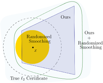
Figure 4: Comparing polyhedral and spherical certificates. Details on left.

It is not immediately obvious how to compare the certificates provided by our method described above and that of RS, since the sets of the space they certify are different. The certified region obtained by RS, $C^{\rm RS}(x)=\{\bar{x}\colon\|x-\bar{x}\|_{2}\leq r(x)\}$, is a sphere (orange ball in Fig. 4). In contrast, our certificate $C_{\lambda}(x)$ from Theorem 4.1 is a polyhedron (resp., blue trapezoid), which, in general, is neither contained in $C^{\rm RS}(x)$, nor a superset of $C^{\rm RS}(x)$. Additionally, our certificate has no standard notion of size, unlike other work on elliptical certificates [13], making a size comparison non-trivial. To overcome these difficulties, we will evaluate two notions of attack size: in the first, we will compare the $\ell_{2}$ norms of successful attacks projected onto our polyhedron, and in the second, we will compare the minimum $\ell_{2}$ norm required for a successful attack. We will then combine our method with RS to get the best of both worlds, i.e., the green shape in Fig. 4. In the following, we detail and present both these evaluations on the MNIST [27] dataset, with each image normalized to unit $\ell_{2}$ norm.

Comparison along Projection on $C_{\lambda}(x)$. For the first case, we investigate the question: Are there perturbations for which our method is certifiably correct, but Randomized Smoothing fails? For an input point $x$, we can answer this question in the affirmative by obtaining an adversarial example $\bar{x}$ for $g^{\rm RS}$ such that $\bar{x}$ lies inside our certified set $C_{\lambda}(x)$. Then, this perturbation $v=x-\bar{x}$ is certified by our method, but has $\ell_{2}$ norm larger than $r^{\rm RS}(x)$ (by definition of the RS certificate).

To obtain such adversarial examples, we first train a standard CNN classifier $f$ for MNIST, and then use RS to obtain the classifier $g^{\rm RS}_{\sigma}$. Then, for any $(x,y)$, we perform projected gradient descent to obtain $\bar{x}=x^{T}$ by performing the following steps $T$ times, starting with $x^{0}\leftarrow x$:

$$\textup{I.}\ x^{t}\leftarrow{\rm Proj}_{B_{\ell_{2}}(x,\epsilon)}\Big{(}x^{t-1}+\eta\nabla_{x}{\rm Loss}(g^{\rm RS}_{\sigma}(x^{t}),y)\Big{)}\qquad\textup{II.}\ x^{t}\leftarrow{\rm Proj}_{C_{\lambda}(x)}(x^{t})$$ (13)

Unlike the standard PGD attack (step I), the additional projection (step II) is not straightforward, and requires us to solve a quadratic optimization problem, which can be found in Appendix F. We can now evaluate $g^{\rm RS}_{\sigma}$ on these perturbations to empirically estimate the robust accuracy over $C_{\lambda}$, i.e.,

$${\rm ProjectionRobustAcc}(\epsilon)=\Pr_{x,y\sim p_{\rm MNIST}}\Big{(}\exists\bar{x}\in B_{\ell_{2}}(x,\epsilon)\cap C_{\lambda}(x)\text{ such that }g^{\rm RS}(\bar{x})\neq y\Big{)}.$$

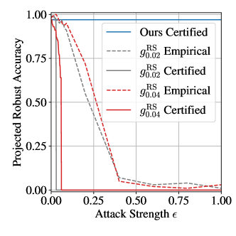
Figure 5: Comparing RS with Our method for adversarial perturbations computed by repeating Steps I, II (13).

The results are plotted in Fig. 5, as the dotted curves. We also plot the certified accuraciesFootnote 6 for comparison, as the solid curves. We see that the accuracy certified by RS drops below random chance (0.1) around $\epsilon=0.06$ (solid red curve). Similar to other certified defenses, RS certifies only a subset of the true robust accuracy of a classifier in general. This true robust accuracy curve is pointwise upper-bounded by the empirical robust accuracy curve corresponding to any attack, obtained via the steps $\textup{I},\textup{II}$ described earlier (dotted red curve). We then see that even the upper-bound drops below random chance around $\epsilon=0.4$, suggesting that this might be a large enough attack strength so that an adversary only constrained in $\ell_{2}$ norm is able to fool a general classifier. However, we are evaluating attacks lying on our certified set and it is still possible to recover the true class (blue solid curve), albeit by our specialized classifier $g_{\lambda}$ suited to the data structure. Additionally, this suggests that our certified set contains useful class-specific information – this is indeed true, and we present some qualitative examples of images in our certified set in Appendix F.

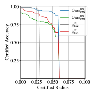
Figure 6: Comparing Certified Accuracy after combining our method with RS.

To summarize, we have numerically demonstrated that exploiting data structure in classifier design leads to certified regions capturing class-relevant regions beyond $\ell_{p}$-balls.

Comparison along $\ell_{2}$ balls. For the second case, we ask the question: Are there perturbations for which RS is certifiably correct, but our method is not? When an input point $x$ has a large enough RS certificate $r^{\rm RS}(x)\geq r_{0}$, some part of the sphere $B_{\ell_{2}}(x,r^{\rm RS}(x))$ might lie outside our polyhedral certificate $C_{\lambda}(x)$ (blue region in Fig. 4). In theory, the minimum $r_{0}$ required can be computed via an expensive optimization program that we specify in Appendix F. In practice, however, we use a black-box attack [8] to find such perturbations. We provide qualitative examples in Appendix F.

Combining Our Method with RS. We now improve our certified regions using randomized smoothing. For this purpose, we treat our classifier $g_{\lambda}$ as the base classifier $f$ in (12), to obtain ${\rm Smooth_{\sigma}(g_{\lambda})}$ (abbreviated as ${\rm Ours}^{\rm RS}_{\sigma}$). We then plot the $\ell_{2}$ certified accuracyFootnote 6 [10, Sec 3.2.2] in Fig. 6, where note that, as opposed to Fig. 5, the attacks are not constrained to lie on our certificate anymore. We observe that not only does randomized smoothing enable us to obtain a $\ell_{2}$ robustness certificate, we can in fact slightly improve (note the $10\times$ zoom on the $x$-axis compared to Fig. 5) over the certificates obtained by RS on its own (blue curve vs. red curve in Fig. 6).

As a final remark, we note that our objective in Fig. 6 was simply to explore RS as a method for obtaining an $\ell_{2}$ certificate for our method, and we did not tune our method or RS for performance. In particular, we believe that a wide array of tricks developed in the literature for improving RS performance [38, 41, 57] could be employed to improve the curves in Fig. 6.

6 Conclusion and Discussion

This paper studies conditions under which a robust classifier exists for a given classification task. We showed that concentration of the data distribution on small subsets of the ambient space is necessary for any classifier to be robust to small adversarial perturbations, and that a stronger notion of concentration is sufficient. We then studied a special concentration data distribution, that of data distributed near low-dimensional linear subspaces. For this special case of our results, we constructed a provably robust classifier, and then experimentally evaluated its benefits w.r.t. known techniques.

For our concentration results, our proof techniques utilize tools from high-dimensional probability, and have the same flavor as recent impossibility results for adversarial robustness [11, 44, 43]. Our geometric treatment of the dual optimization problem is similar to the literature on sparse-representation [12, 20] and subspace clustering [46, 47, 59, 24], which is concerned with the question of representing a point $x$ by the linear combination of columns of a dictionary $\mathbf{S}$ using sparse coefficients $c$. As mentioned in Section 4, there exist geometric conditions on $\mathbf{S}$ such that all such candidate vectors $c$ are subspace-preserving, i.e., for all the indices $i$ in the support of $c$, it can be guaranteed that $s_{i}$ belongs to the correct subspace. On the other hand, the question of classification of a point $x$ in a union of subspaces given by the columns of $\mathbf{S}$, or subspace classification, has also been studied extensively in classical sparse-representation literature [56, 55, 6, 26, 58, 60, 18, 36, 22, 31]. The predominant approach is to solve an $\ell_{1}$ minimization problem to obtain coefficients $c$ so that $x=\mathbf{S}c+e$, and then predict the subspace that minimizes the representation error. Various global conditions can be imposed on $\mathbf{S}$ to guarantee the success of such an approach [56], and its generalizations [14, 15]. Our work differs from these approaches in that we aim to obtain conditions on perturbations to $x$ that ensure accurate classification, and as such we base our robust classification decision upon properties of solutions of the dual of the $\ell_{1}$ problem.

Our work is also related to recent empirical explorations on obtaining robust classifiers by denoising a given input $x$ of any adversarial corruptions, before passing it to a classifier [42, 35]. However, such approaches lack theoretical guarantees, and might be broken using specialized attacks [37]. Similarly, work on improving the robustness of deep network-based classifiers by adversarial training off the data-manifold can be seen as an empirical generalization of our attack model [23, 34, 62, 32]. More generally, it has been studied how adversarial examples relate to the underlying data-manifold [48, 25, 33]. Recent work also studies the robustness of classification using projections onto a single subspace [3, 2, 40]. Such works are close to us in spirit, as they use projections onto a single low-dimensional linear subspace to provide robustness certificates. [3] study an the attack model of bounded $\ell_{2},\ell_{\infty}$ attacks, and they provide robustness certificates by obtaining guarantees on the distortion of a data-point $x$ as it is projected onto a single linear subspace using a projection matrix $\Pi$. In contrast, our work can be seen as projecting a perturbed point onto a union of multiple low-dimensional subspaces. The resultant richer geometry allows us to obtain more general certificates.

One of the limitations of our work is that we always assume access to a clean dataset $\mathbf{S}$ lying perfectly on the union of low-dimensional linear subspaces. In reality, one might only have access to noisy samples. In light of existing results on noisy subspace clustering [53], an immediate future direction is to adapt our guarantees to support noise in the training data. While the assumption of low-dimensional subspace structure in $\mathbf{S}$ enables us to obtain novel unbounded robustness certificates, real world datasets might not satisfy this structure. We hope to mitigate this limitation by extending our formulation to handle data lying on a general image manifold in the future.

Appendix A Proof of Theorem 2.1

We will make the technical assumption in Section 2 precise. Recall that all quantities are normalized so that $\mathcal{X}$ is an $\ell_{2}$ ball of radius $1$, i.e., $\mathcal{X}=B_{\ell_{2}}(0,1)$. Recall that $q_{k}\colon\mathcal{X}\to\mathbb{R}_{\geq 0}$ denotes the conditional distribution for class $k\in\mathcal{Y}$, having support $Q_{k}$. We will assume that there is a sufficient gap between the supports and the boundary of the domain, i.e., $Q_{k}\subseteq B_{\ell_{2}}(0,c)$, and that the $\ell_{2}$-adversarial attack has strength $\epsilon\leq c$, for some constant $c$.

See 2.1

Proof.

Note that the definition (1) of $(\epsilon,\delta)$-robustness may be rewritten as

$$R(f,\epsilon) =\sum_{k}p_{X|Y}(X\text{admits an $\epsilon$-adversarial example}|Y=k)p_{Y}(y=k)$$

$$=\sum_{k}q_{k}(\{x\in\mathcal{X}\colon\exists\bar{x}\in B(x,\epsilon)\text{ such that }f(\bar{x})\neq k\})p_{Y}(y=k),$$ (14)

where $q(S)$ denotes the $q$-measure of the set $S$. We are given $f$ such that $R(f,\epsilon)\leq\delta$, and we want to find a set $S\subseteq\mathcal{X}$ over which $p$ concentrates.

$$R(f,\epsilon)\leq\delta$$

$$\implies\sum_{k}q_{k}(\{x\in\mathcal{X}\colon\exists\bar{x}\in B(x,\epsilon)\cap\mathcal{X}\text{ such that }f(\bar{x})\neq k\})p_{Y}(y=k)\leq\delta$$ (15)

Since $\sum_{k}p_{Y}(y=k)=1$, the LHS in (15) is a convex combination, and we have

$$\implies\exists\hat{k}\ q_{\bar{k}}(\{x\in\mathcal{X}\colon\exists\bar{x}\in B(x,\epsilon)\cap\mathcal{X}\text{ such that }f(\bar{x})\neq\hat{k}\})\leq\delta,$$ (16)

$$\implies q_{\bar{k}}(U)\leq\delta,\text{ where }$$

$$U=\{x\in\mathcal{X}\colon\exists\bar{x}\in B(x,\epsilon)\cap\mathcal{X}\text{ such that }f(\bar{x})\neq\hat{k}\}.$$

We will express $q_{\hat{k}}(U)$ in terms of the classification regions of $f$.

Let $A\subseteq\mathcal{X}$ denote the region where the classifier predicts $\hat{k}$, i.e. $A=\{x\in\mathcal{X}\colon f(x)=\hat{k}\}$. Define $A^{-\epsilon}$ to be the set of all points in $A$ at a $\ell_{2}$ distance atleast $\epsilon$ from the boundary, i.e. $A^{-\epsilon}=\{x\in A\colon B(x,\epsilon)\subseteq A\}$. Now consider any point $x\in\mathcal{X}$. We have the following 4 mutually exclusive, and exhaustive cases:

1. $x$ lies outside $A$, i.e., $x\not\in A$. In this case, $x\in U$ trivially as $f(x)\neq k$.

2. $x\in A$, and the entire $\epsilon$-ball around $x$ lies inside $A$, i.e., $B(x,\epsilon)\subseteq A$. In this case, every point in the $\epsilon$-ball around $x$ is classified into class $\hat{k}$, and $x$ has no $\epsilon$-adversarial example for class $\hat{k}$. Note that the set of all these points is $A^{-\epsilon}$ by definition.

3. $x\in A$, and some portion of the $\epsilon$-ball around $x$ lies outside $A$, i.e., $B(x,\epsilon)\not\subseteq A$, and, there is a point $\bar{x}\in B(x,\epsilon)\cap\mathcal{X}$ such that $f(\bar{x})\neq k$. In this case, $\bar{x}$ is an adversarial example for $x$, and $\bar{x}\in U$.

4. $x\in A$, and some portion of the $\epsilon$-ball around $x$ lies outside $A$, i.e., $B(x,\epsilon)\not\subseteq A$, but there is no point $\bar{x}\in B(x,\epsilon)\cap\mathcal{X}$ such that $f(\bar{x})\neq k$. This can happen only when for all $\bar{x}\in B(x,\epsilon)\setminus A$ we have $\bar{x}\not\in\mathcal{X}$. In other words, any $\epsilon$ perturbation that takes $x$ outside $A$, also takes it outside the domain $\mathcal{X}$. This implies that $B(x,\epsilon)\not\subseteq\mathcal{X}$, which in turn means that the distance of $x$ from the boundary of $\mathcal{X}$ is atmost $\epsilon$.

We see that $U$ comprises of the points covered in cases (1) and (3). Recall that we assumed that any point having distance less than $0.1$ to the boundary of $\mathcal{X}$ does not lie in the support of $q_{\bar{k}}$. But all points covered in case (4) lie less than $\epsilon$-close to the boundary, and $\epsilon\leq 0.1$. This implies that $q_{\bar{k}}$ assigns $0$ measure to the points covered in case (4). Together, cases (1), (3) and (4) comprise the set $(\mathcal{X}\setminus A)\cup(A\setminus A^{-\epsilon})$. Thus, we have shown

$$q_{\hat{k}}(U)=q_{\hat{k}}(\mathcal{X}\setminus A^{-\epsilon})$$

$$\implies q_{\hat{k}}(A^{-\epsilon})\geq 1-\delta.$$ (17)

Next, we will show that the set $A^{-\epsilon}$ is exponentially small, by appealing to the Brunn-Minkowski inequality, which states that for compact sets $E,F\subset\mathbb{R}^{n}$,

$${\rm Vol}(E+F)^{\frac{1}{n}}\geq{\rm Vol}(E)^{\frac{1}{n}}+{\rm Vol}(F)^{\frac{1}{n}},$$

where ${\rm Vol}$ is the $n$-dimensional volume in $\mathbb{R}^{n}$, and $E+F$ denotes the minkowski sum of the sets $E$ and $F$. Applying the inequality with $E=A^{-\epsilon}$ and $F=B_{\ell_{2}}(0,\epsilon)$, we have

$${\rm Vol}(A^{-\epsilon}+B_{\ell_{2}}(0,\epsilon))^{\frac{1}{n}} \geq{\rm Vol}(A^{-\epsilon})^{\frac{1}{n}}+{\rm Vol}(B_{\ell_{2}}(0,\epsilon))^{\frac{1}{n}}$$

$$\implies{\rm Vol}(A)^{\frac{1}{n}} \geq{\rm Vol}(A^{-\epsilon})^{\frac{1}{n}}+\epsilon{\rm Vol}(B_{\ell_{2}}(0,1))^{\frac{1}{n}}$$

$$\implies{\rm Vol}(A)^{\frac{1}{n}} \geq{\rm Vol}(A^{-\epsilon})^{\frac{1}{n}}+\epsilon{\rm Vol}(A)^{\frac{1}{n}}$$

$$\implies\frac{{\rm Vol}(A^{-\epsilon})^{\frac{1}{n}}}{{\rm Vol}(A)^{\frac{1}{n}}} \leq(1-\epsilon)$$

$$\implies{\rm Vol}(A^{-\epsilon}) \leq{\rm Vol}(A)(1-\epsilon)^{n}\leq{\rm Vol}(A)\exp(-\epsilon n)$$

$$\implies{\rm Vol}(A^{-\epsilon}) \leq c_{1}\exp(-c_{2}\epsilon),$$ (18)

where $c_{1}$ is the volume of the unit ball in $n$ dimensions, and $c_{2}=n$.

From (17) and (18), we see that $q_{\bar{k}}$ is $(\epsilon,\delta)$-concentrated. Additionally, if the classes are balanced, we can use the fact that every term of (15) can be atmost $K\delta$, and apply the above reasoning for each class to conclude that each $q_{k}$ is $(\epsilon,K\delta)$-concentrated. ∎

Appendix B Proof of Theorem 3.1

See 3.1

Proof.

For each $k\in\{1,2,\ldots,K\}$, let $S_{k}$ be the support of the conditional density $q_{k}$. Recall that $S^{+\epsilon}$ is defined to be the $\epsilon$-expansion of the set $S$. Define $C_{k}$ to be the $\epsilon$-expanded version of the concentrated region $S_{k}$ but removing the $\epsilon$-expanded version of all other regions $S_{k^{\prime}}$, as

$$C_{k}=\left(S_{k}^{+\epsilon}\setminus\cup_{k^{\prime}\neq k}S^{+\epsilon}_{k^{\prime}}\right)\cap\mathcal{X}.$$

We will use these regions to define our classifier $f\colon\mathcal{X}\to\{1,2,\ldots,K\}$ as

$$f(x)=\begin{cases}1,&\text{ if }x\in C_{1}\\ 2,&\text{ if }x\in C_{2}\\ \vdots\\ K,&\text{ if }x\in C_{K}\\ 1,&\text{ otherwise }\end{cases}.$$

We will show that $R(f,\epsilon)\leq\delta+\gamma$, which can be recalled to be

$$R(f,\epsilon)=\sum_{k}q_{k}(\{x\in\mathcal{X}\colon\exists\bar{x}\in B(x,\epsilon)\cap\mathcal{X}\text{ such that }f(\bar{x})\neq k\})p_{Y}(y=k).$$

In the above expression, the $q_{k}$ mass is over the set of all points $x\in\mathcal{X}$ that admit an $\epsilon$-adversarial example for the class $k$, as

$$U_{k}=\{x\in\mathcal{X}\colon\exists\bar{x}\in B(x,\epsilon)\cap\mathcal{X}\text{ such that }f(\bar{x})\neq k\}.$$ (19)

Define $C^{-\epsilon}_{k}$ to be the set of points in $C_{k}$ at a distance atleast $\epsilon$ from the boundary of $C_{k}$ as $C^{-\epsilon}_{k}=\{x\in C_{k}\colon B(x,\epsilon)\subseteq C_{k}\}$. For any point $x\in U_{k}$, we can find $\bar{x}\in B(x,\epsilon)$ from (19) such that $\bar{x}\not\in C_{k}$, showing that $x\not\in C_{k}^{-\epsilon}$. Thus, $U_{k}$ is a subset of the complement of $C_{k}^{-\epsilon}$, i.e., $U_{k}\subseteq\mathcal{X}\setminus C_{k}^{-\epsilon}$, and we have

$$R(f,\epsilon)=\sum_{k}q_{k}(U_{k})p_{Y}(y=k)\leq\sum_{k}(1-q_{k}(C_{k}^{-\epsilon}))p_{Y}(y=k).$$

Now we will need to show a few properties of the $\epsilon$-contraction. Firstly, for a set $M=N\cap O$, we have $M^{-\epsilon}=N^{-\epsilon}\cap O^{-\epsilon}$, which can be seen as

$$M^{-\epsilon} =\{x\colon x\in M,B(x,\epsilon)\subseteq M\}$$

$$=\{x\colon x\in N,x\in O,B(x,\epsilon)\subseteq N,B(x,\epsilon)\subseteq O\}=N^{-\epsilon}\cap O^{-\epsilon}.$$

Secondly, for a set $M=N^{c}$, where $c$ denotes complement, we have $M^{-\epsilon}=(N^{+\epsilon})^{c}$. This can be seen as

$$M^{-\epsilon} =\{x\colon x\in M,B(x,\epsilon)\subseteq M\}=\{x\colon x\not\in N,B(x,\epsilon)\subseteq N^{c}\}$$

$$=\{x\colon x\not\in N,\forall x^{\prime}\in B(x,\epsilon)\ x^{\prime}\not\in N\}$$

$$=\{x\colon\forall x^{\prime}\in B(x,\epsilon)\ x^{\prime}\not\in N\}$$

$$\implies(M^{-\epsilon})^{c} =\{x\colon\exists x^{\prime}\in B(x,\epsilon)\ x^{\prime}\in N\}$$

$$=N^{+\epsilon}.$$

Thirdly, for a set $M=N\setminus O$, we have $M^{-\epsilon}=(N\cap O^{c})^{-\epsilon}=N^{-\epsilon}\cap(O^{c})^{-\epsilon}$ by the first property, and then $N^{-\epsilon}\cap(O^{c})^{-\epsilon}=N^{-\epsilon}\cap(O^{+\epsilon})^{c}$ by the second property. This implies

$$(N\setminus O)^{-\epsilon}=N^{-\epsilon}\setminus O^{+\epsilon}.$$

Fourthly, for a set $M=N\cup O$, we have $M^{c}=N^{c}\cap O^{c}$. Taking $\epsilon$-contractions, and applying the first and second properties, we get $M^{+\epsilon}=N^{+\epsilon}\cup O^{+\epsilon}$. Applying the above properties to $C_{k}^{-\epsilon}$, we have

$$C_{k}^{-\epsilon} =\left(S_{k}^{+\epsilon}\setminus\cup_{k^{\prime}\neq k}S^{+\epsilon}_{k^{\prime}}\right)^{-\epsilon}\cap\mathcal{X}^{-\epsilon}$$

$$=\left(S_{k}\setminus\big{(}\cup_{k^{\prime}\neq k}S^{+\epsilon}_{k^{\prime}}\big{)}^{+\epsilon}\right)\cap\mathcal{X}^{-\epsilon}$$

$$=\left(S_{k}\setminus\cup_{k^{\prime}\neq k}S^{+2\epsilon}_{k^{\prime}}\right)\cap\mathcal{X}^{-\epsilon}.$$

Recall that $q_{k}(\mathcal{X}^{-\epsilon})=q(\mathcal{X})=1$ by the support assumption. Hence, we have

$$q_{k}(C_{k}^{-\epsilon})=q_{k}\left(S_{k}\setminus\cup_{k^{\prime}\neq k}S^{+2\epsilon}_{k^{\prime}}\right)=q_{k}(S_{k})-q_{k}\left(\cup_{k^{\prime}\neq k}S^{+2\epsilon}_{k^{\prime}}\right)\geq(1-\delta)-\gamma$$

$$\implies 1-q_{k}(C_{k}^{-\epsilon})\leq\delta+\gamma.$$

Finally, as $\sum_{k}p_{Y}(y=k)=1$, we have $R(f,\epsilon)\leq\delta+\gamma$ by convexity. ∎

Appendix C Proofs for Example 3.1

Let $\theta_{0}\leq\pi/2$. We will show that the following classifier $f$ is robust in the setting of Example 3.1:

$$f(x)=\begin{cases}1,&\text{ if }x^{\top}P\geq\theta_{0}\\ 2,&\text{otherwise}\end{cases}.$$

Let $C_{1}=\{x\in\mathbb{S}^{n-1}\colon x^{\top}P\geq\theta_{0}\}$ be the set of points classified into class $1$ by $f$. Similarly, let $C_{2}=\mathbb{S}^{n-1}\setminus C_{1}$ be the set of points classified into class $2$. The robust risk of $f$ (measured w.r.t. perturbations in the geodesic distance $d$) can be expanded as

$$R_{d}(f,\epsilon)=0.5q_{1}(d^{+\epsilon}(C_{2}))+0.5q_{2}(d^{+\epsilon}(C_{1})),$$ (20)

where $d^{+\epsilon}(S)$ denotes the $\epsilon$-expansion of the set $S$ under the distance $d$. Let $\epsilon\leq\theta_{0}$ (otherwise, the first term is $1/2$). Recall that the class conditional $q_{1}$ is defined as

$$q_{1}(x)=\begin{cases}\frac{1}{c_{\psi}}\frac{\psi(d(x,P))}{\sin^{n-2}d(x,P)},&\text{ if }d(x,P)\leq\theta_{0}\\ 0,&\text{ otherwise }\end{cases},$$

where $c_{\psi}$ is a normalizing constant which ensures that $q_{1}$ integrates to $1$, i.e., $c_{\psi}=\int_{\mathbb{S}^{n-1}}q_{1}$. Then, $q_{2}$ was defined to be uniform over the complement of the support of $q_{1}$, i.e. $q_{2}={\rm Unif}(\{x\in\mathbb{S}^{n-1}\colon d(x,P)>\theta_{0}\})$.

We can expand the first term of Eq. 20 as

$$q_{1}(d^{+\epsilon}(C_{2})) =q_{1}(d^{+\epsilon}(C_{2})\setminus C_{2})+q_{1}(C_{2})$$

$$=q_{1}(\{x\colon 0<d(x,C_{2})\leq\epsilon\})+0.$$

Now for any $x\not\in C_{2}$, we have $d(x,C_{2})=\theta_{0}-d(x,P)$. Hence, $\{x\colon 0<d(x,C_{2})\leq\epsilon\}=\{x\colon 0.1-\epsilon\leq d(x,P)<\theta_{0}\}$. Let $\theta(x)$ denote the angle that $x$ makes with $P$. Then, the geodesic distance is $d(x,P)=\theta(x)$. The earlier set is the same as the set of all points satisfying $\theta_{0}-\epsilon\leq\theta(x)<1$. This is nothing but the $\epsilon$-base of the hyper-spherical cap having angle $\theta_{0}$.

We continue,

$$q_{1}(\{x\colon\theta_{0}-\epsilon<d(x,P)\leq\theta_{0}) =q_{1}(\{x\colon\theta_{0}-\epsilon\leq\theta(x)<\theta_{0}\})$$

With a change of variables, the above can be evaluated as

$$q_{1}(\{\theta_{0}-\epsilon\leq\theta(x)<\theta_{0}\}) =\frac{1}{c_{\psi}}\int_{\theta_{0}-\epsilon\leq\theta(x)<\theta_{0}}\frac{\psi(d(x,P))}{\sin(d(x,P))^{n-2}}dx$$

$$=\frac{1}{c_{\psi}}\int^{\theta_{0}}_{\theta_{0}-\epsilon}\frac{\psi(\theta)}{(\sin\theta)^{n-2}}\mu_{n-2}(\{x\in\mathbb{S}^{n-1}\colon\theta(x)=\theta\})d\theta,$$

where $\mu_{n-2}$ is the $n-2$-dimensional volume ($n-1$-dimensional surface area). Now, $\mu_{n-2}(\{x\in\mathbb{S}^{n-1}\colon\theta(x)=\theta\})$ is nothing but the volume of an slice of the hypersphere $\mathbb{S}^{n-1}$. This slice is in itself a hypersphere in $\mathbb{R}^{n-1}$, having radius $\sin\theta$. Thus, its volume is the same as the volume of the $\mathbb{S}^{n-2}$, scaled by $(\sin\theta)^{n-2}$. We continue,

$$\int^{\theta_{0}}_{\theta_{0}-\epsilon}\frac{\psi(\theta)}{(\sin\theta)^{n-2}}\mu_{n-2}(\{x\in\mathbb{S}^{n-1}\colon\theta(x)=\theta\})d\theta =\int^{\theta_{0}}_{\theta_{0}-\epsilon}\frac{\psi(\theta)}{(\sin\theta)^{n-2}}(\sin\theta)^{n-2}d\theta$$

$$=\int^{\theta_{0}}_{\theta_{0}-\epsilon}\psi(\theta)d\theta$$

For illustration, we can take $\psi(\theta)=1$, giving $q_{1}(d^{+\epsilon}(C_{1}))=\epsilon/C$ from the above integral, with $c_{\psi}=\int_{0}^{\theta_{0}}\psi(\theta)d\theta=\theta_{0}=\theta_{0}$.

We can now follow the same process as above, and expand the Eq. 20 as

$$q_{2}(d^{+\epsilon}(C_{1}))=\mu_{n-1}(\{x\colon\theta_{0}\leq\theta(x)\leq\theta_{0}+\epsilon),$$

where $\mu_{n-1}$ is again the $n-1$-dimensional volume. We use the following formula [30] for the surface area of a hyperspherical cap (valid when $\alpha\ \leq\pi/2$):

$$\mu_{n-1}(\{x\colon 0\leq\theta(x)\leq\alpha\})=m(\alpha)\overset{\rm def}{=}0.5\mu_{n-1}(\mathbb{S}^{n-1})I_{\sin^{2}\alpha}\left(\frac{n-1}{2},\frac{1}{2}\right),$$

where $I(\cdot,\cdot)$ is the incomplete regularized beta function. Letting $d_{\theta_{0}}=m(\pi/2)+m(\pi/2)-m(\theta_{0})$, we continue,

$$q_{2}(d^{+\epsilon}(C_{1}))=\begin{cases}\frac{1}{d_{\theta_{0}}}\big{(}m(\theta_{0}+\epsilon)-m(\theta_{0})\big{)},&\text{ if }\epsilon+\theta_{0}\leq\pi/2\\ \frac{1}{d_{\theta_{0}}}\big{(}m(\pi/2)+m(\pi/2)-m(\theta_{0}+\epsilon-\pi/2)\big{)},&\text{ if }\pi/2\leq\epsilon+\theta_{0}\leq\pi\\ \frac{1}{d_{\theta_{0}}},&\text{ else }\end{cases}.$$

The risk from class $1$ dominates till $\epsilon$ reaches around $\pi/2$, then the risk from class $2$ shoots up. We plot the resultant risk in Fig. 7 (left).

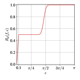
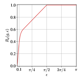
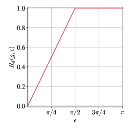
Figure 7: Robust risk for classifiers for concentrated distributions on the sphere $\mathbb{S}^{n-1}$, for dimension $n=100$. (Left): A plot of $R_{d}(f,\epsilon)$ w.r.t $p_{1}$. As $\epsilon$ grows from $0$ to $0.1$, class $1$ is the major contributor to the risk. At $\epsilon=0.1$, all points in class $1$ admit an adversarial perturbation, taking them to class $2$. As $\epsilon$ grows further, the risk for class $2$ grows slowly, till $\epsilon$ reaches close to $\pi/2$, after which it blows up abruptly due to the high-dimensional fact that most of the mass of the uniform distribution lies near the equator of the sphere. (Middle): A plot of $R_{d}(g,\epsilon)$ w.r.t. $p_{2}$. As we make the support of the concentrated class larger, the distribution admits a classifier $g$ with slightly improved robustness for smaller $\epsilon$ values ($\leq 0.1$). (Right): A plot of $R_{d}(g,\epsilon)$ w.r.t. $p_{3}$: Finally, as both class conditionals are made concentrated, the classifier $g$ becomes quite robust.

Having presented the basic construction, we now comment on how Example 3.1 can be generalized. Firstly, we can vary the support of $q_{1}$, to have it cover a different fraction of the sphere. For instance, we can set $\theta_{0}=\pi/2$ to get a modified $q_{1}$ as

$$q^{\prime}_{1}(x)=\begin{cases}\frac{1}{C}\frac{1}{\sin^{n-2}d(x,P)},&\text{ if }d(x,P)\leq\pi/2\\ 0,&\text{ otherwise }\end{cases},$$

and let $q^{\prime}_{2}$ be uniform over the complement of the support of $q^{\prime}_{1}$. Along with balanced classes (i.e., $P(Y=1)=P(Y=2)=1/2$), this gives the data distribution $p_{2}$. The robust classifier would now be given by the half-space $\{x\colon d(x,P)\leq\pi/2\}$. The risk over $p_{2}$ can be computed as earlier, and is plotted in Fig. 7 (middle).

We can take this example further, and make both $q_{1}$ and $q_{2}$ concentrated. This can be done, for instance, by setting $q^{\prime\prime}_{1}=q_{1}$, and setting $q^{\prime\prime}_{2}$ as follows:

$$q^{\prime\prime}_{2}(x)=\begin{cases}\frac{1}{C}\frac{1}{\sin^{n-2}d(x,-P)},&\text{ if }d(x,-P)\leq\pi/2\\ 0,&\text{ otherwise }\end{cases},$$

where $-P$ is the antipodal point of $P$. As both class conditionals are now concentrated, the halfspace separating their supports becomes quite robust. This can be seen in the Fig. 7 (right).

Lastly, $\psi$ can be taken to be a rapidly decaying function for even greater concentration and lesser robust risk, e.g., $\psi(\theta)=\exp(-\theta)$.

Appendix D Proofs for Example 4.1

See 4.1

It would be helpful to have Fig. 8 in mind for what follows.

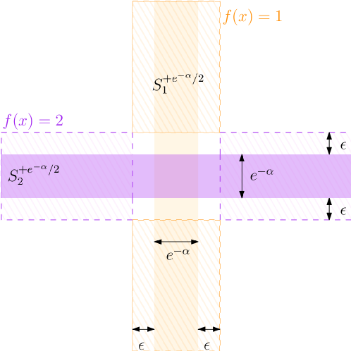
Figure 8: A plot of $q_{1}$ (orange), $q_{2}$ (violet) and the decision boundaries of $f$ (dashed).

We will demonstrate that the classifier $f$ illustrated in Fig. 8 has low robust risk. We define $f$ for any $x\in B_{\infty}(0,1)$, as follows (let $\gamma=e^{-\alpha}$):

$$f(x)=\begin{cases}1,&\text{ if }|x_{1}|\leq\gamma/2+\epsilon,|x_{2}|\geq\gamma/2+\epsilon\\ 2,&\text{ if }|x_{2}|\leq\gamma/2+\epsilon,|x_{1}|\geq\gamma/2+\epsilon\\ 1,&\text{otherwise}\end{cases}.$$

The reason for splitting the cases for predicting $1$ into two subcases, is because we will only need to analyse the first subcase and the second will not contribute to the robust risk.

Defining $U_{1}$ to be the set of all points $x$ which admit an adversarial example for the class $1$, i.e. $U_{1}=\{x\colon\exists\bar{x}\text{ such that }\|\bar{x}-x\|_{2}\leq\epsilon,f(\bar{x})=2\}$. It is clear that

$$U_{1}\subseteq\{x\colon|x_{1}|\geq\gamma/2\text{ or }|x_{2}|\leq\gamma/2+2\epsilon\}.$$

$U_{2}$ is defined analogously, and

$$U_{2}\subseteq\{x\colon|x_{2}|\geq\gamma/2\text{ or }|x_{1}|\leq\gamma/2+2\epsilon\}.$$

Now, $R(f,\epsilon)=0.5q_{1}(U_{1})+0.5q_{2}(U_{2})$. We look at the first term, and simplify an upper bound:

$$q_{1}(U_{1}) \leq q_{1}(\{x\colon|x_{1}|\geq\gamma/2\text{ or }|x_{2}|\leq\gamma/2+2\epsilon)$$

$$\leq q_{1}(\{x\colon|x_{1}|\geq\gamma/2\})+q_{1}(\{x\colon|x_{2}|\leq\gamma/2+2\epsilon)$$

$$=0+q_{1}(\{x\colon|x_{2}|\leq\gamma/2+2\epsilon\}).$$ (21)

Now, recall that $q_{1}={\rm Unif}(\{x\colon|x_{1}|\leq\gamma/2\})$, hence the expression in (21) evaluates to

$$q_{1}(\{x\colon|x_{2}|\leq\gamma/2+2\epsilon\}) =\frac{1}{{\rm Vol}(\{x\colon|x_{1}|\leq\gamma/2\})}{\rm Vol}(\{x\colon|x_{2}|\leq\gamma/2+2\epsilon,|x_{1}|\leq\gamma/2\})$$

$$=\frac{1}{2^{n-1}\gamma}2^{n-2}\cdot(\gamma+4\epsilon)\cdot\gamma$$

$$=0.5\gamma+2\epsilon$$

The situation for $q_{2}$ is symmetric, and hence $q_{2}(U_{2})=0.5(\gamma+4\epsilon)$. Adding them together, we see that the robust risk is upper bounded by

$$R(f,\epsilon)\leq 0.5(e^{-\alpha}+4\epsilon)$$

For the strong concentration parameters, note that the support of $q_{1}$, i.e., $S_{1}=\{x\colon|x_{1}|\leq\gamma/2,\|x\|_{\infty}\leq 1\}$ has volume $\gamma 2^{n-1}=2^{n-1}\exp(-\alpha)$. Hence, $q_{1}$ is $(\alpha,0)$ concentrated over $S_{1}$. Similarly, $q_{2}$ is $(\alpha,0)$-concentrated over $S_{2}=\{x\colon|x_{2}|\leq\gamma/2,\|x\|_{\infty}\leq 1\}$. Finally,

$$q_{1}(S_{2}^{+2\epsilon}) =q_{1}(\{\|x\|_{\infty}\leq 1,\|x_{1}\|\leq\gamma/2,\|x_{2}\|\leq\gamma/2+2\epsilon\})$$

$$=2^{n-2}\gamma(\gamma+4\epsilon)\gamma^{-1}2^{1-n}$$

$$=0.5\gamma+2\epsilon$$

Appendix E Proof of Theorem 4.1

See 4.1

Proof.

Let $\lambda x^{\prime}\in C(x)$ as defined in (8). There exist $f\in F(x),v\in V(x)$ such that $\lambda x^{\prime}=f+v$. We will show that the projection of $\lambda x^{\prime}$ onto $F$ is given by $f$. Recall that

$$A_{\lambda}(x^{\prime})=\{t_{i}\colon\langle t_{i},d^{*}_{\lambda}(x^{\prime})\rangle=1\},\text{ where }d^{*}_{\lambda}(x^{\prime})={\rm Proj}_{K^{\circ}}(\lambda x^{\prime}).$$ (22)

Choose any $z\in K^{\circ}$. Recall that ${\rm Proj}_{K^{\circ}}(\lambda x^{\prime})=\min_{z\in K^{\circ}}\|z-\lambda x^{\prime}\|_{2}$. Consider the objective,

$$\|z-\lambda x^{\prime}\|_{2}^{2}=\|(z-f)-v\|_{2}^{2}=\|z-f\|_{2}^{2}+\|v\|_{2}^{2}-2\langle z-f,v\rangle.$$ (23)

We will show that $\langle z-f,v\rangle$ is negative. Consider any $t_{i}\in A_{\lambda}(x)$, and observe that $\langle z,t_{i}\rangle\leq 1$, as $z\in K^{\circ}$. However, from the definition of $F(x)$ recall that $\langle f,t_{i}\rangle=1$. This implies that $\langle z-f,t_{i}\rangle\leq 0$. Using the fact that $v\in V(x)$, we expand the inner product as

$$\langle z-f,v\rangle=\sum_{t_{i}\in A_{\lambda}(x)}\alpha_{i}\langle z-f,t_{i}\rangle\leq 0.$$ (24)

Using (24) in (23) to obtain

$$\|z-\lambda x^{\prime}\|_{2}^{2}\geq\|z-f\|_{2}^{2}+\|v\|_{2}^{2}\geq 0.$$ (25)

The minimizer above is obtained at $z=f\in C(x)$, and hence we have shown that for all $\lambda x^{\prime}\in C(x)$, ${\rm Proj}_{K^{\circ}}(\lambda x^{\prime})=f$. Finally, $d^{*}_{\lambda}(x^{\prime})={\rm Proj}_{K^{\circ}}(\lambda x^{\prime})=f\in F(x)$. The theorem statement then follows from the definition of $F(x)$. ∎

Appendix F Further Experimental Details and Qualitative Examples

F.1 Comparison along Projection on $C_{\lambda}$

In this section, we will provide more details on attacking a classifier with perturbations that lie on our certified set $C_{\lambda}$.

Details of the Projection Step II in (13)

Recall from Theorem 4.1 that $C_{\lambda}(x)$ is defined as the Minkowski sum of the face $F_{\lambda}(x)$ (9) and the cone $V_{\lambda}(x)$ (10). Given an iterate $x^{t}$, we can compute its projection onto $C_{\lambda}(x^{0})$ by solving the following optimization problem

$${\rm Proj}_{C_{\lambda}(x^{0})}(x^{t}) =\operatorname*{arg\,min}_{x}\|x^{t}-x\|_{2}\text{ s.t. }x\in C_{\lambda}(x^{0})$$

Now every $x\in C_{\lambda}(x^{0})$ can be written as $x=d+v$ where $d\in F(x^{0}),v\in V(x^{0})$. $d$ is such that $t^{\top}d=1$ for all $t_{i}\in A_{\lambda}(x^{0})$, and $t^{\top}d\leq 1$ otherwise. Then, $v$ is such that $v=\sum_{t_{i}\in A_{\lambda}(x^{0})}\alpha_{i}t_{i}$ for some $\alpha_{i}\geq 0$. Recall that $T=[t_{1},t_{2},\ldots,t_{2M}]$ denotes the matrix containing the training data-points as well as their negations. Let the matrix $A_{1}\in\mathbb{R}^{d\times|A_{\lambda}(x^{t})|}$ contain all the columns of $T$ in $A_{\lambda}(x^{t})$ and let $A_{2}\in\mathbb{R}^{d\times(2M-|A_{\lambda}(x^{t})|)}$ contain all the remaining columns. Then the objective of the optimization problem above can be written as

$$\min_{\alpha,d}\left\|x^{t}-A_{1}\alpha-d\right\|^{2}_{2}\text{ s.t. }A_{1}^{\top}d=\mathbf{1},A_{2}^{\top}d\leq\mathbf{1},\alpha\geq\mathbf{0}$$ (26)

(26) is a linearly constrained quadratic program, and can be solved by standard optimization tools. In particular, we use the qp solver from the python cvxopt library.

Visualization of the Certified Set

In Fig. 9, we visualize the set $A_{\lambda}(x)$, i.e., the set of active constraints at the optimal solution of the dual problem, for several $x$ in the MNIST test set. It can be seen that $A_{\lambda}(x)$ contains images of the same digit as $x$ in most cases. This is expected, as taking the majority label among $A_{\lambda}(x)$ gives an accuracy of around $97\%$ (solid blue curve in Fig. 5). Note that all these images $t\in A_{\lambda}(x)$ are also contained in the certified set, $C_{\lambda}(x)$, which can be seen as $t=t+\mathbf{0}$, with $t\in F_{\lambda}(x)$, and $\mathbf{0}\in V_{\lambda}(x)$.

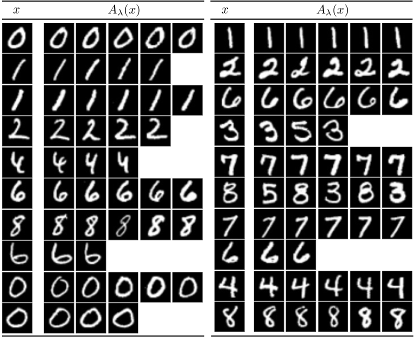
Figure 9: A visualization of the set of active constraints $A_{\lambda}(x)$ for several $x$. Atmost $5$ members of $A_{\lambda}(x)$ are shown for every $x$.

Visualization of Attacks restricted to the Certified Set

In Fig. 10, we visualize the attacks restricted to our certified set $C_{\lambda}$ computed by (13) for the classifier $g^{\rm RS}_{0.02}$. We observe that we can identify the correct digit from most of the attacked images, but the randomized smoothing classifier is incorrect at higher $\epsilon$. A small number of these attacked images are close to the actual class decision boundary, and the class is ambigous. This is expected, both due to the inherent class ambiguity present in some MNIST images, as well as the large $\epsilon$ we are attacking with. For all these images, the prediction of our classifier $g_{\lambda}$ is certified to be accurate. For comparison, the RS certificate is unable to certify anything beyond $\epsilon\geq 0.06$.

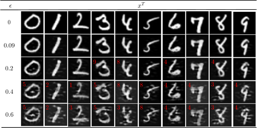
Figure 10: A visualization of attacks on the RS classifier $g^{\rm RS}_{0.02}$ restricted to our certified set $C_{\lambda}$ obtained by (13). Different rows plot different attack strengths $\epsilon$. Whenever an image is misclassified, the red annotation on the top left shows the class predicted by $g^{\rm RS}_{0.02}$.

F.2 Comparison along $\ell_{2}$ balls

Exact Certification for $g_{\lambda}$

In this section, we first state and prove Theorem 4.1 that allows us to exactly compute the $\ell_{2}$ certified radius for our classifier $g_{\lambda}$ at any point $x$.

Lemma F.1.

For all $x^{\prime}\in C(x)$ as defined in Theorem 4.1, we have $g_{\lambda}(x^{\prime})=g_{\lambda}(x)$. Additionally, for all $\|v\|_{2}\leq r_{0}(x)$ we have $g_{\lambda}(x+v)=g_{\lambda}(x)$, where

$$\begin{split}r_{0}(x)=&\quad\;\;\min_{\mathbf{u}}\quad-\langle x,\mathbf{u}\rangle\\ &\quad\text{sub. to}\quad\|\mathbf{u}\|_{2}=1,\quad\langle\mathbf{u},t_{i}\rangle\leq 0\ \forall t_{i}\in A_{\lambda}(x),\quad\langle\mathbf{u},v\rangle\leq 1\ \forall v\in{\rm ext}(F(x)),\end{split}$$ (27)

where ${\rm ext}(F(x))$ is the set of extreme points of the polyhedron $F(x)$.

Discussion

Before presenting the proof, let us ponder over the result. We see that (27) involves solving an optimization problem having as many constraints as the number of extreme points of the polyhedron $F(x)$. In general, this can be very large in high dimensions, and hence computationally inefficient to compute. As a result, while Lemma F.1 provides an exact certificate in theory, it is hard to use in practice without further approximations.

Proof.

Recall that given a set $A_{\lambda}(x)$, the polyhedron $C(x)$ is defined in (8) as

$$C(x)=F(x)+V(x),$$ (28)

where $F(x)$ is a polyhedron, and $V(x)$ is a cone given as the conic hull of $A_{\lambda}(x)$, i.e., $V(x)=\text{cone}(A_{\lambda}(x))$. We want to find the size $r(x)$ of the largest $\ell_{2}$ ball centered at $x$, i.e., $B(x,r(x))$, that can be inscribed within $C(x)$. From convex geometry [4], we know that any polyhedron can be described as an intersection over halfspaces obtained from its polar, $C^{\circ}$ as

$$C(x)=\cap_{\mathbf{u}\in C^{\circ}(x)}H^{-}(\mathbf{u},0),$$ (29)

where $H^{-}(\mathbf{u},0)=\{x\colon\langle\mathbf{u},x\rangle\leq 0\}$. The distance of $x$ from the boundary of $C(x)$ is the same as the smallest distance of $x$ from any halfspace in (29). However, this distance is simply

$$\text{dist}(x,H^{-}(\mathbf{u},0))=-\left\langle x,\frac{\mathbf{u}}{\|\mathbf{u}\|_{2}}\right\rangle.$$ (30)

In other words, we can expressing $C(x)$ as the intersection over halfspaces whose normals lie in $C^{\circ}(x)$, i.e.,

$$r(x)=\left(\min_{\mathbf{u}}-\langle x,\mathbf{u}\rangle,\text{ sub. to }\|\mathbf{u}\|_{2}=1,\mathbf{u}\in C^{\circ}(x)\right).$$ (31)

All that is left is to obtain a description of $C^{\circ}(x)$. This can be done by first expressing $C(x)$ in a standard form, as

$$C(x)=\text{conv}(\text{ext}(F(x)))+\text{cone}(A_{\lambda}(x)),$$ (32)

where $\text{ext}(F(x))$ denotes the extreme points of the polyhedron $F(x)$, $\text{conv}(\cdot)$ denotes the convex hull and $\text{cone}(\cdot)$ denotes the conic hull. Now we can apply a theorem in convex geometry to obtain the polar ([4, Th. 2.79]) as

$$C^{\circ}(x)=\left\{\mathbf{u}\colon\begin{array}[]{l}\langle\mathbf{u},t_{i}\rangle\leq 0\ \forall t_{i}\in A_{\lambda}(x)\\ \langle\mathbf{u},v\rangle\leq 1\ \forall v\in\text{ext}(F(x))\end{array}\right\}$$ (33)

Combining (31) and (33), we obtain the lemma statement. Finally, we note that as Theorem 4.1 shows that $A_{\lambda}(x^{\prime})=A_{\lambda}(x)$ for all $\lambda x^{\prime}\in C(x)$, and the classifier $g_{\lambda}(x)$ is purely a function of $A_{\lambda}(x)$, we have that $g_{\lambda}(x^{\prime})=g_{\lambda}(x)$ for all $\lambda x^{\prime}\in C(x)$. ∎

Black Box Attacks on $g_{\lambda}$

Since our classifier $g_{\lambda}$ is not explicitly differentiable with respect to its input, we use the HopSkipJump [8] black-box attack to obtain adversarial perturbations that cause a misclassification. The obtained attacked images, and the pertubation magnitude are shown in Fig. 11.

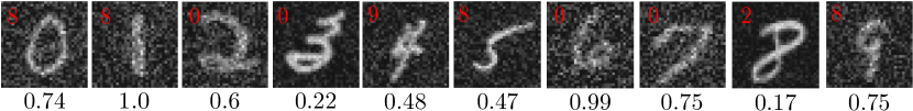
Figure 11: A visualization of attacks on our classifier $g_{\lambda}$ obtained by the HopSkipJump black box attack [8]. The label predicted by $g_{\lambda}$ is shown as a red annotation on the top left. The $\ell_{2}$ perturbation magnitude $\epsilon$ is shown at the bottom. Note that the $\epsilon$ values are not nice fractions because they are set by the HopSkipJump attack using a binary search to find the minimum attack strength that causes a misclassification.

F.3 Details of Randomized Smoothing Certificates

For obtaining the certified accuracy curves using Randomized Smoothing [10] (solid lines in Figs. 5 and 6), we follow the certification and prediction algorithms for RS in [10, Sec 3.2.2]: given a base classifier $f$ and a test image $x$, we use $n_{0}=100$ samples from an isotropic gaussian distribution $\mathcal{N}(0,\sigma)$ to prediction the majority class $g_{\sigma}^{\rm RS}(x)$. We then use $n=100$ samples to estimate the prediction probability $\underline{p_{A}}$ under $\mathcal{N}(0,\sigma)$ with confidence atleast $0.999$. If $\underline{p_{A}}$ is at least $0.5$, we report the certified radius $\sigma\Phi^{-1}(\underline{p_{A}})$. Otherwise, if $\underline{p_{A}}<0.5$, we abstain and return a certified radius of $0$.

Evaluating the Dual Classifier $g_{\lambda}$

We normalize each image in the MNIST dataset to have unit $\ell_{2}$ norm, and resize to $32\times 32$. We pick $10000$ images $s_{i}$ at random from the training set to obtain our data matrix $\mathbf{S}\in\mathbb{R}^{1024\times 10000}$. We now pick a test point $x$, and then solve the dual problem (5) with $\lambda=2$, to obtain the dual solution $d^{*}_{\lambda}(x)$. This allows us to then obtain the set of active constraints $A_{\lambda}(x)$ in (7). Then, we use the majority rule as the aggregate function in (11) to obtain the classfication output from the dual classifier $g_{\lambda}(x)$. We sample $100$ images $x$ uniformly at random from the MNIST test set for generating the curves in Figs. 5 and 6. All experiments are performed on a NVIDIA GeForce RTX 2080 Ti GPU with 12 GB memory.

References

- [1] Anish Athalye, Nicholas Carlini, and David Wagner. Obfuscated gradients give a false sense of security: Circumventing defenses to adversarial examples. In International conference on machine learning, pages 274–283. PMLR, 2018.
- [2] Pranjal Awasthi, Vaggos Chatziafratis, Xue Chen, and Aravindan Vijayaraghavan. Adversarially robust low dimensional representations. In Conference on Learning Theory, pages 237–325. PMLR, 2021.
- [3] Pranjal Awasthi, Himanshu Jain, Ankit Singh Rawat, and Aravindan Vijayaraghavan. Adversarial robustness via robust low rank representations. Advances in Neural Information Processing Systems, 33:11391–11403, 2020.
- [4] Amitabh Basu. Introduction to convexity. Optimization, 52:37, 2019.
- [5] Sébastien Bubeck, Yin Tat Lee, Eric Price, and Ilya Razenshteyn. Adversarial examples from computational constraints. In International Conference on Machine Learning, pages 831–840. PMLR, 2019.
- [6] Raffaele Cappelli, Dario Maio, and Davide Maltoni. Subspace classification for face recognition. In International Workshop on Biometric Authentication, pages 133–141. Springer, 2002.
- [7] Nicholas Carlini, Anish Athalye, Nicolas Papernot, Wieland Brendel, Jonas Rauber, Dimitris Tsipras, Ian Goodfellow, Aleksander Madry, and Alexey Kurakin. On evaluating adversarial robustness. arXiv preprint arXiv:1902.06705, 2019.
- [8] Jianbo Chen, Michael I Jordan, and Martin J Wainwright. Hopskipjumpattack: A query-efficient decision-based attack. In 2020 ieee symposium on security and privacy (sp), pages 1277–1294. IEEE, 2020.
- [9] Ping-yeh Chiang, Renkun Ni, Ahmed Abdelkader, Chen Zhu, Christoph Studer, and Tom Goldstein. Certified defenses for adversarial patches. In 8th International Conference on Learning Representations (ICLR 2020)(virtual). International Conference on Learning Representations, 2020.
- [10] Jeremy Cohen, Elan Rosenfeld, and Zico Kolter. Certified adversarial robustness via randomized smoothing. In International Conference on Machine Learning, pages 1310–1320. PMLR, 2019.
- [11] Elvis Dohmatob. Generalized no free lunch theorem for adversarial robustness. In International Conference on Machine Learning, pages 1646–1654. PMLR, 2019.
- [12] David L Donoho and Michael Elad. Optimally sparse representation in general (nonorthogonal) dictionaries via l1 minimization. Proceedings of the National Academy of Sciences, 100(5):2197–2202, 2003.
- [13] Francisco Eiras, Motasem Alfarra, Philip Torr, M Pawan Kumar, Puneet K Dokania, Bernard Ghanem, and Adel Bibi. Ancer: Anisotropic certification via sample-wise volume maximization. Transactions of Machine Learning Research, 2022.
- [14] Ehsan Elhamifar and René Vidal. Robust classification using structured sparse representation. In CVPR 2011, pages 1873–1879. IEEE, 2011.
- [15] Ehsan Elhamifar and René Vidal. Block-sparse recovery via convex optimization. IEEE Transactions on Signal Processing, 60(8):4094–4107, 2012.
- [16] Gamaleldin Elsayed, Shreya Shankar, Brian Cheung, Nicolas Papernot, Alexey Kurakin, Ian Goodfellow, and Jascha Sohl-Dickstein. Adversarial examples that fool both computer vision and time-limited humans. Advances in neural information processing systems, 31, 2018.
- [17] Alhussein Fawzi, Hamza Fawzi, and Omar Fawzi. Adversarial vulnerability for any classifier. Advances in neural information processing systems, 31, 2018.
- [18] Lunke Fei, Yong Xu, Xiaozhao Fang, and Jian Yang. Low rank representation with adaptive distance penalty for semi-supervised subspace classification. Pattern Recognition, 67:252–262, 2017.
- [19] Marc Fischer, Maximilian Baader, and Martin Vechev. Certified defense to image transformations via randomized smoothing. Advances in Neural Information Processing Systems, 33:8404–8417, 2020.
- [20] Simon Foucart and Holger Rauhut. An invitation to compressive sensing. In A mathematical introduction to compressive sensing, pages 1–39. Springer, 2013.
- [21] Chuan Guo, Mayank Rana, Moustapha Cisse, and Laurens van der Maaten. Countering adversarial images using input transformations. In International Conference on Learning Representations, 2018.
- [22] Kang-hua Hui, Chun-li Li, and Lei Zhang. Sparse neighbor representation for classification. Pattern Recognition Letters, 33(5):661–669, 2012.
- [23] Charles Jin and Martin Rinard. Manifold regularization for locally stable deep neural networks. arXiv preprint arXiv:2003.04286, 2020.
- [24] Mustafa D Kaba, Chong You, Daniel P Robinson, Enrique Mallada, and Rene Vidal. A nullspace property for subspace-preserving recovery. In Marina Meila and Tong Zhang, editors, Proceedings of the 38th International Conference on Machine Learning, volume 139 of Proceedings of Machine Learning Research, pages 5180–5188. PMLR, 18–24 Jul 2021.
- [25] Marc Khoury and Dylan Hadfield-Menell. On the geometry of adversarial examples. arXiv preprint arXiv:1811.00525, 2018.
- [26] Jorma Laaksonen et al. Subspace classifiers in recognition of handwritten digits. Helsinki University of Technology, 1997.
- [27] Yann LeCun. The mnist database of handwritten digits. http://yann.lecun.com/exdb/mnist/, 1998.
- [28] Alexander Levine and Soheil Feizi. (de) randomized smoothing for certifiable defense against patch attacks. Advances in Neural Information Processing Systems, 33:6465–6475, 2020.
- [29] Chun-Guang Li, Chong You, and René Vidal. On geometric analysis of affine sparse subspace clustering. IEEE Journal of Selected Topics in Signal Processing, 12(6):1520–1533, 2018.
- [30] Shengqiao Li. Concise formulas for the area and volume of a hyperspherical cap. Asian Journal of Mathematics & Statistics, 4(1):66–70, 2010.
- [31] Wei Li, Eric W Tramel, Saurabh Prasad, and James E Fowler. Nearest regularized subspace for hyperspectral classification. IEEE Transactions on Geoscience and Remote Sensing, 52(1):477–489, 2013.
- [32] Wei-An Lin, Chun Pong Lau, Alexander Levine, Rama Chellappa, and Soheil Feizi. Dual manifold adversarial robustness: Defense against lp and non-lp adversarial attacks. Advances in Neural Information Processing Systems, 33:3487–3498, 2020.
- [33] Xingjun Ma, Bo Li, Yisen Wang, Sarah M Erfani, Sudanthi Wijewickrema, Grant Schoenebeck, Dawn Song, Michael E Houle, and James Bailey. Characterizing adversarial subspaces using local intrinsic dimensionality. In International Conference on Learning Representations, 2018.
- [34] Seyed-Mohsen Moosavi-Dezfooli, Alhussein Fawzi, Jonathan Uesato, and Pascal Frossard. Robustness via curvature regularization, and vice versa. In Proceedings of the IEEE/CVF Conference on Computer Vision and Pattern Recognition, pages 9078–9086, 2019.
- [35] Seyed-Mohsen Moosavi-Dezfooli, Ashish Shrivastava, and Oncel Tuzel. Divide, denoise, and defend against adversarial attacks. arXiv preprint arXiv:1802.06806, 2018.
- [36] Imran Naseem, Roberto Togneri, and Mohammed Bennamoun. Linear regression for face recognition. IEEE transactions on pattern analysis and machine intelligence, 32(11):2106–2112, 2010.
- [37] Zhonghan Niu, Zhaoxi Chen, Linyi Li, Yubin Yang, Bo Li, and Jinfeng Yi. On the limitations of denoising strategies as adversarial defenses. arXiv preprint arXiv:2012.09384, 2020.
- [38] Ambar Pal and Jeremias Sulam. Understanding noise-augmented training for randomized smoothing. Transactions on Machine Learning Research, 2023.
- [39] Nicolas Papernot, Patrick McDaniel, Xi Wu, Somesh Jha, and Ananthram Swami. Distillation as a defense to adversarial perturbations against deep neural networks. In 2016 IEEE symposium on security and privacy (SP), pages 582–597. IEEE, 2016.
- [40] Samuel Pfrommer, Brendon G Anderson, and Somayeh Sojoudi. Projected randomized smoothing for certified adversarial robustness. 2022.
- [41] Hadi Salman, Jerry Li, Ilya Razenshteyn, Pengchuan Zhang, Huan Zhang, Sebastien Bubeck, and Greg Yang. Provably robust deep learning via adversarially trained smoothed classifiers. Advances in Neural Information Processing Systems, 32, 2019.
- [42] Pouya Samangouei, Maya Kabkab, and Rama Chellappa. Defense-gan: Protecting classifiers against adversarial attacks using generative models. In International Conference on Learning Representations, 2018.
- [43] Ludwig Schmidt, Shibani Santurkar, Dimitris Tsipras, Kunal Talwar, and Aleksander Madry. Adversarially robust generalization requires more data. Advances in neural information processing systems, 31, 2018.
- [44] Ali Shafahi, W Ronny Huang, Christoph Studer, Soheil Feizi, and Tom Goldstein. Are adversarial examples inevitable? arXiv preprint arXiv:1809.02104, 2018.
- [45] Ali Shafahi, Mahyar Najibi, Mohammad Amin Ghiasi, Zheng Xu, John Dickerson, Christoph Studer, Larry S Davis, Gavin Taylor, and Tom Goldstein. Adversarial training for free! Advances in Neural Information Processing Systems, 32, 2019.
- [46] Mahdi Soltanolkotabi and Emmanuel J Candes. A geometric analysis of subspace clustering with outliers. The Annals of Statistics, 40(4):2195–2238, 2012.
- [47] Mahdi Soltanolkotabi, Ehsan Elhamifar, and Emmanuel J Candes. Robust subspace clustering. The annals of Statistics, 42(2):669–699, 2014.
- [48] David Stutz, Matthias Hein, and Bernt Schiele. Disentangling adversarial robustness and generalization. In Proceedings of the IEEE/CVF Conference on Computer Vision and Pattern Recognition, pages 6976–6987, 2019.
- [49] Jeremias Sulam, Ramchandran Muthukumar, and Raman Arora. Adversarial robustness of supervised sparse coding. Advances in neural information processing systems, 33:2110–2121, 2020.
- [50] Christian Szegedy, Wojciech Zaremba, Ilya Sutskever, Joan Bruna, Dumitru Erhan, Ian Goodfellow, and Rob Fergus. Intriguing properties of neural networks. arXiv preprint arXiv:1312.6199, 2013.
- [51] Dimitris Tsipras, Shibani Santurkar, Logan Engstrom, Alexander Turner, and Aleksander Madry. Robustness may be at odds with accuracy. arXiv preprint arXiv:1805.12152, 2018.
- [52] René Vidal, Yi Ma, and S Shankar Sastry. Generalized Principal Component Analysis. Springer, 2016.
- [53] Yu-Xiang Wang and Huan Xu. Noisy sparse subspace clustering. In International Conference on Machine Learning, pages 89–97. PMLR, 2013.
- [54] Eric Wong, Leslie Rice, and J Zico Kolter. Fast is better than free: Revisiting adversarial training. In International Conference on Learning Representations, 2019.
- [55] John Wright, Yi Ma, Julien Mairal, Guillermo Sapiro, Thomas S Huang, and Shuicheng Yan. Sparse representation for computer vision and pattern recognition. Proceedings of the IEEE, 98(6):1031–1044, 2010.
- [56] John Wright, Allen Y Yang, Arvind Ganesh, S Shankar Sastry, and Yi Ma. Robust face recognition via sparse representation. IEEE transactions on pattern analysis and machine intelligence, 31(2):210–227, 2008.
- [57] Greg Yang, Tony Duan, J Edward Hu, Hadi Salman, Ilya Razenshteyn, and Jerry Li. Randomized smoothing of all shapes and sizes. In International Conference on Machine Learning, pages 10693–10705. PMLR, 2020.
- [58] Jianchao Yang, Jiangping Wang, and Thomas Huang. Learning the sparse representation for classification. In 2011 IEEE International Conference on Multimedia and Expo, pages 1–6. IEEE, 2011.
- [59] Chong You and René Vidal. Geometric conditions for subspace-sparse recovery. In International Conference on Machine Learning, pages 1585–1593. PMLR, 2015.
- [60] Guoxian Yu, Guoji Zhang, Zili Zhang, Zhiwen Yu, and Lin Deng. Semi-supervised classification based on subspace sparse representation. Knowledge and Information Systems, 43(1):81–101, 2015.
- [61] Bohang Zhang, Du Jiang, Di He, and Liwei Wang. Rethinking lipschitz neural networks for certified l-infinity robustness. arXiv preprint arXiv:2210.01787, 2022.
- [62] Shufei Zhang, Kaizhu Huang, Jianke Zhu, and Yang Liu. Manifold adversarial training for supervised and semi-supervised learning. Neural Networks, 140:282–293, 2021.