Magnetocaloric effect in $\mathrm{Cu}_{3}$-type compounds using the Heisenberg antiferromagnetic model in a triangular ring

Abstract

In this work we present a theoretical investigation into an antiferromagnetically coupled spin system, specifically ${\rm Cu}_{3}-X$ ($\mathrm{X=As,Sb}$), which exhibits an isosceles triangular configuration or slightly distorted equilateral triangular configuration, as previously identified in reference [Phys. Rev. Lett. 96, 107202 (2006)]. This system can be effectively represented by the Heisenberg model on a triangular structure, taking into account the exchange interaction, the Dzyaloshinskii-Moriya interaction, g-factors and external magnetic field, as delineated in the aforementioned reference. By using numerical approach we explore both zero-temperature and finite-temperature behaviors of a ${\rm Cu}_{3}$-like antiferromagnetically coupled spin system. At zero temperature, the system displays a 1/3 quasi-plateau magnetization, when the magnetic field is varied. Moreover, we place particular emphasis on magnetic properties including magnetization, magnetic susceptibility, entropy, and specific heat at finite temperatures. Furthermore, we investigate the magnetocaloric effect as a function of an externally imposed magnetic field, oriented both parallel and perpendicular to the plane of the triangular structure. Interestingly, these configurations demonstrate remarkably similar behavior for both orientations of the magnetic field. Our investigation also includes an analysis of the adiabatic curve, the Grüneisen parameter, and the variation in entropy when applied or removed the magnetic field. The magnetocaloric effect is found to be more prominent in low the temperature region, typically at $T\sim 1$K, for both parallel and perpendicular magnetic fields at $\sim 4.5$T and $\sim 5$T, respectively.

I Introduction

The study of spin systems with antiferromagnetic coupling has drawn significant attention in the field of condensed matter physics. These systems exhibit interesting features that arise from the interplay of various factors that can be investigated through their magnetic properties. Moreover, understanding the characteristics of these systems helps to clarify their potential applications in areas such as magnetocaloric materials and spintronics

The Magnetocaloric Effect (MCE) is a phenomenon that has been studied extensively due to its potential applications in magnetic refrigeration and cooling technologies. Initially observed in the late 19th century, it refers to the change in temperature that occurs when a magnetic material is subjected to a varying magnetic field, a phenomenon resulting from the intrinsic magnetic properties of the material [1, 2]. The reversibility of this effect has been confirmed in later studies, sparking significant interest [2]. The MCE has been observed in a variety of materials, such as rare earth alloys, magnetic oxides, and transition metals, with notable instances of a giant magnetocaloric effect (GMCE) driven by structural transitions [3, 4]. In 1951, Darby and colleagues made a pioneering step in the field by designing a two-stage magnetocaloric regenerator using materials with different Curie points, achieving temperature down to the final values as low as 3mK at an induction of 0.42T [5].

The concept of magnetic refrigeration at room temperature was introduced almost a century after the discovery of MCE. In 1976, Brown developed an efficient refrigeration system using gadolinium, marking a significant advancement [6]. Following this, in the late 90s, Gschneidner discovered GMCE at room temperature in gadolinium-germanium-silicon alloys (Ga-Ge-Si) [7]. Around the same time, Zimm proposed a prototype showcasing the feasibility of magnetic refrigeration near room temperature [8]. These developments led to substantial experimental and theoretical research on bulk $\mathrm{(Mn,Fe)_{2}(P,Si)}$-based GMCE materials [7, 9, 10, 11, 12].

Nanoscale materials with GMCE have gained attention due to their high surface-to-volume ratio, enhanced interactions, and rapid thermal response. These characteristics make them valuable for temperature control applications. Examples of such applications include a room-temperature thermal diode [13], a self-pumping magnetic cooling device using Mn-Zn ferrite nanoparticles that achieves efficient energy conservation without external energy input [14], a magnetic cooling device based on a ferrofluid thermomagnetic that can effectively transfer heat over large distances [15], control of ferrofluid droplets in microfluidics [16], and a magnetostructural phase transition in Ni-Mn-Ga films showing a strong MCE at low magnetic fields [17]. Other applications involve gadolinium thick films for energy conversion mechanisms [10, 11] and biomedical applications like magnetic hyperthermia [18] and efficient drug delivery via nanocarriers [19].

Furthermore, the study of magnetic materials has attracted significant attention due to their wide range of potential technological applications in fields such as spintronics, nanoscale engineering, and biomedicine. This has prompted investigations on $S=1/2$ antiferromagnetic triangular spin rings, which might be ideal for observing peculiar quantum magnetization due to two doublets. Compounds investigated include spin-frustrated $(\mathrm{VO})_{3}^{6+}$-triangle-sandwiching octadecatungstates as molecular magnets, displaying unusual magnetization jumps due to predicted half-step or 1/3-plateau magnetization [20]. Experiments on a $\mathrm{Cu}_{3}$ nanomagnet revealed half-step magnetization, hysteresis loops, and an asymmetric magnetization between negative and positive field in fast sweeping external field, which can be ascribed to an adiabatic change of mgnetization[21]. Whereas in [22] was investigated the spin-electric coupling. The $S=1/2$ spin triangle clusters were also investigated, revealing that the magnetization behavior and spin configurations are significantly affected by the diamagnetic heteroatom ($X={\rm As}$ and ${\rm Sb}$) [23]. These clusters show potential for implementing spin-based quantum gates [24]. Bouammali et al. [25] explored the antisymmetric exchange in a tri-copper(II) complex, highlighting its origins, theoretical implications, and potential for more advanced electronic structure calculations. A spin-frustrated trinuclear copper complex based on triaminoguanidine demonstrates strong antiferromagnetic interactions with negligible antisymmetric exchange [26]. Several other studies have also examined triangular copper structures [27, 28, 29, 30, 31].

On the other hand, theoretical investigations to explore various properties of nanomagnets or magnetic molecular clusters, beyond experimental results, are highly significant. For instance, Kowalewska and Szałowski conducted a theoretical study of the magnetocaloric properties of $V6$, a polyoxovanadate molecular magnet. Their research, using numerical diagonalization and field ensemble formalism, uncovered highly tunable magnetocaloric effects [32]. KarǏová et al. studied the magnetization in antiferromagnetic spin-1/2 XXZ Heisenberg clusters, demonstrating additional magnetization plateaux due to quantum interaction and an enhanced magnetocaloric effect near magnetization shifts [33]. Reference [34] employed exact diagonalization to examine the spin-1/2 Hamiltonian for coupled isosceles Heisenberg triangles, yielding a zero-temperature quantum phase transition diagram and a magnetization profile. They also analyzed the thermodynamic behavior and MCE. Another theoretical study was conducted on a $\mathrm{Cu}_{5}$ pentameric molecule using a spin-1/2 Heisenberg model, which explored the thermodynamic properties, phase diagram, magnetization, and magnetocaloric effects [35]. Theoretical study of the MCE in paramagnetic $\mathrm{PrNi}_{2}$ revealed an unexpected inverse effect due to an anomalous increase in magnetic entropy at low temperatures [36]. Several other theoretical investigations can be found in references therein [32, 33, 34, 35, 36].

In this context, a system of interest is ${\rm Cu}_{3}-X$ ($\mathrm{X=As,Sb}$), which adopts an isosceles triangular or slightly distorted equilateral triangular configuration. Previously, Choi et al. [21, 23, 24] have established that the behavior of this system can be effectively described by the Heisenberg model on a triangular structure, incorporating elements such as exchange interaction, Dzyaloshinskii-Moriya interaction, g-factors, and external magnetic fields. Exploring the magnetic properties and thermodynamic behavior of this ${\rm Cu}_{3}$-like spin system is important as it helps us understand its fundamental characteristics and identify potential advantages for its applications.

The article is organized as follows: in sec. 2 we present the model and analyze some fundamental properties. In sec. 3 we explore main thermodynamic properties. Whereas in sec.4 we discuss the magnetocaloric effect. Finally in sec. 5 we devote our conclusions.

II Model

In this work, we aim to explore the thermodynamics and magnetic properties of a triangular cluster ${\rm Na}_{9}[{\rm Cu}_{3}{\rm Na}_{3}({\rm H}_{2}{\rm O})_{9}(\alpha-X{\rm W}_{9}{\rm O}_{33})_{2}]$ (where $X={\rm As}$ and ${\rm Sb}$) hereinafter referred to as the {${\rm Cu}_{3}-X$} system[21]. The compound under consideration contains three copper atoms, each of which loses two electrons to form a Cu(II) or $\mathrm{Cu}^{+2}$ ion. The electron loss in Cu(II) ions occurs from both the 4s and one of the 3d orbitals, resulting in a single unpaired electron and a net magnetic moment with a spin of $S=1/2$; this behavior can be adequately described by the Heisenberg model within the framework of an isosceles triangular spin ring [21, 23, 24]. Consequently, we adopt the Hamiltonian, as presented in previous work [21, 23, 24], which characterizes ${\rm Cu}_{3}$-like compounds, as follows

$$\mathbf{H}= \sum_{j=1}^{3}\sum_{\alpha=x,y,z}J_{j,j+1}^{\alpha}S_{j}^{\alpha}S_{j+1}^{\alpha}$$

$$+\sum_{j=1}^{3}\Bigl{[}{\bf D}_{j,j+1}\cdot\left({\bf S}_{j}\times{\bf S}_{j+1}\right)+\mu_{B}{\bf S}_{j}\cdot\mathbf{g}_{j}\cdot{\bf B}_{j}\Bigr{]},$$ (1)

where $S_{j}^{\alpha}$ denotes the spin-1/2 components of localized ${\rm Cu}_{3}$-like spin with $\alpha=\{x,y,z\}$, and $J_{j,j+1}^{\alpha}$ (simplified as $J_{j}^{\alpha}$) represents the exchange interaction parameters between site $j$ and $j+1$ for each component (for schematic view see reference [21, 23, 24]). The second term refers to the Dzyaloshinskii-Moriya interaction vector ${\bf D}_{j,j+1}$ denoted as ${\bf D}_{j,j+1}=(D_{j,j+1}^{x},D_{j,j+1}^{y},D_{j,j+1}^{z})$. The site-dependent $g$-factors are defined as $\mathbf{g}_{j}=(g_{j}^{x},g_{j}^{y},g_{j}^{z})$, while the last term corresponds to the magnetic field $\mathbf{B}$, which we assume to be independent of the spin site on the triangle. Here, $\mu_{B}$ denotes the Bohr magneton. The specific parameters were obtained using Electron Spin Resonance (ESR) data [21, 23, 24], and these parameters are reproduced in table 1 for both compounds. It is worth mentioning that only ${\bf D}_{1,2}=(D,D,D)$ is isotropic, while ${\bf D}_{2,3}$ and ${\bf D}_{3,1}$ contribute solely to the $z$-component, expressed as ${\bf D}_{2,3}={\bf D}_{3,1}=(0,0,D)$. Other interactions, such as the crystal field effect and magneto-crystalline anisotropy, were disregarded in this study because their contributions are not deemed highly relevant, as supported by references[21, 31].

For convenience, we express the Hamiltonian (1) in units of kelvin (K). Hence, let us redefine $\mu_{B}$ as $\hat{\mu}_{B}=\frac{\mu_{B}}{k_{B}}=0.6717156644$ K/T, where $k_{B}$ denotes the Boltzmann constant. Therefore, the magnetic field $\mathbf{B}$ is conveniently measured in tesla (T) units. This can be equivalent to setting the Boltzmann constant as $k_{B}=1$, implying that, for the sake of simplicity, all calculation will be expressed in units of $k_{B}$.

Magnetic parameters	notation	{${\rm Cu}_{3}-{\rm As}$}	{${\rm Cu}_{3}-{\rm Sb}$}
$J_{1,2}^{x}=J_{1,2}^{y}$	$J_{1}$	$4.50$ K	$4.49$ K
$J_{1,2}^{z}$	$J_{1}^{z}$	$4.56$ K	$4.54$ K
$J_{2,3}^{x}=J_{2,3}^{y}=J_{3,1}^{x}=J_{3,1}^{y}$	$J_{2}$	$4.03$ K	$3.91$ K
$J_{2,3}^{z}=J_{3,1}^{z}$	$J_{2}^{z}$	$4.06$ K	$3.96$ K
$D_{1,2}^{z}=D_{2,3}^{z}=D_{3,1}^{z}$	$D$	$0.529$ K	$0.517$ K
$D_{1,2}^{x}=D_{1,2}^{y}$	$D$	$0.529$ K	$0.517$ K
$g_{1}^{x}=g_{1}^{y}$	$g_{1}$	$2.25$	$2.24$
$g_{2}^{x}=g_{2}^{y}$	$g_{2}$	$2.10$	$2.11$
$g_{3}^{x}=g_{3}^{y}$	$g_{3}$	$2.40$	$2.40$
$g_{1}^{z}=g_{2}^{z}=g_{3}^{z}$	$g_{z}$	$2.06$	$2.07$

Table 1: Magnetic parameters of the {${\rm Cu}_{3}-X$} compounds, where $X$ denotes either As or Sb, as extracted from reference[23].

III Thermodynamics quantities

The eigenvalues of the above mentioned Hamiltonian (1), can be obtained by direct numerical diagonalization. More details about the energy spectra can be found in reference [21, 23, 24], so let us assume that the eigenvalues can be expressed as follows

$$\mathbf{U}\mathbf{H}\mathbf{U}^{-1}=\mathbf{E}={\rm diag}\left(\varepsilon_{1},\varepsilon_{2},\cdots,\varepsilon_{8}\right),$$ (2)

where $\mathbf{U}$ is an $8\times 8$ matrix that diagonalizes the Hamiltonian (1). It is important to note that this matrix, which naturally depends on the Hamiltonian parameters, can only be obtained numerically for a fixed magnetic field.

Thus, the partition function can symbolically be represented by:

$$\mathcal{Z}={\rm tr}\left({\rm e}^{-\mathbf{E}/T}\right)=\sum_{i=1}^{8}{\rm e}^{-\varepsilon_{i}/T}.$$ (3)

Here, the eigenvalues $\varepsilon_{i}$ (in kelvin units) depend on the Hamiltonian parameters provided in table 1, as well as the magnetic field $\mathbf{B}$ (in tesla), while $T$ represents the temperature of the system (in kelvin). In theory, any physical quantity can be derived from the partition function (3). However, as the eigenvalues can only be obtained numerically, physical quantities that require derivatives, such as magnetization and magnetic susceptibility among others, must be calculated with caution. Numerical derivatives may not always provide accurate results, hence it is advisable to avoid them as much as possible. Therefore, we will combine numerical and analytical calculations to safely obtain all physical quantities.

In this regard, the free energy can be denoted by the expression

$$f=-T\ln(\mathcal{Z}).$$ (4)

It should be noted that the free energy is also represented in units of $k_{B}$.

III.1 Internal energy

The first quantity we will discuss is the internal energy, as it directly influences the magnitude of the magnetocaloric effect. As previously stated, the eigenvalues of the Hamiltonian can be obtained using the parameters listed in table 1 and a fixed magnetic field. Formally, the average internal energy can be represented as:

$$U=\langle\mathbf{H}\rangle=\frac{1}{\mathcal{Z}}{\rm tr}\left\{\mathbf{H}{\rm e}^{-\mathbf{H}/T}\right\}=\frac{1}{\mathcal{Z}}\sum_{i=1}^{8}\varepsilon_{i}{\rm e}^{-\varepsilon_{i}/T}.$$ (5)

For the purposes of our discussion, we will focus on the ${\rm Cu}_{3}-{\rm As}$ compound. The ${\rm Cu}_{3}-{\rm Sb}$ compound exhibits analogous characteristics because the parameters given in table 1 are quite similar.

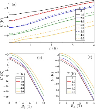
Figure 1: (a) Internal energy $U$ as a function of temperature, solid lines corresponds to $B_{\perp}$, while dashed lines corresponds to $B_{\parallel}$. (b-c) Internal energy $U$ as a function of perpendicular and parallel external magnetic field, respectively. These plots are specifically for the ${\rm Cu}_{3}-{\rm As}$ compound.

Figure 1a depicts the internal energy ($U$) as a function of temperature, assuming a constant parallel external magnetic field to the triangle plane (solid line) and perpendicular to it (dashed line). The internal energy varies slightly between the parallel and perpendicular magnetic fields. Although, as the magnetic field increases, the discrepancy becomes more pronounced. In contrast, panels (b and c) show the internal energy as a function of the parallel and perpendicular external magnetic fields, respectively. These figures assume several fixed temperatures, as specified inside the panel. At zero temperature, we observe a significant change of internal energy at $B_{\parallel}\approx 4.5$ T. Above this magnetic field, the system aligns entirely parallel to the magnetic field, while for $B_{\parallel}\lesssim 4.5$ T, the configuration comprises two aligned spins and a third with opposite alignment. We observe similar behavior when the external magnetic field acts perpendicularly to the triangular plane, but the shift occurs at a slightly higher magnetic field, $B_{\perp}\approx 5$ T. This similarity has previously been observed in energy spectra and zero-temperature magnetization [21, 23, 24]. As temperature increases, this curvature smooths out. In the absence of an external magnetic field, these spin moments are oriented randomly, leading to a higher internal energy state. When an external magnetic field is applied, the spins align with the field, reducing the internal energy of the compound. This variation of energy manifests as a change in the compound temperature, representing the core of the magnetocaloric effect.

III.2 Entropy

Entropy calculation is relevant as it plays a crucial role in the MCE. Essentially serving as the "driving force" to understand both the direct and inverse MCE, which we will discuss subsequently. As such, entropy is fundamental to understand the mechanism of MCE and is pertinent in applications such as magnetic refrigeration. Consequently, entropy can be derived from the internal energy with the following relation

$$\mathcal{S}=\frac{\langle\mathbf{H}\rangle-f}{T}.$$ (6)

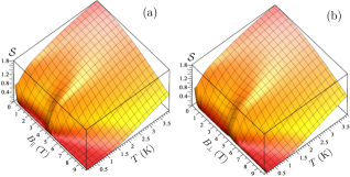
Figure 2: (a) Entropy ${\cal S}$ in the plane of temperature (in kelvin) and parallel external magnetic field (tesla). (b) Entropy ${\cal S}$ in the plane of temperature (in kelvin) and perpendicular external magnetic field (tesla). These visualizations are based on the ${\rm Cu}_{3}-{\rm As}$ compound.

In Fig. 2a the entropy is illustrated in the plane of temperature (in kelvin) and parallel external magnetic field (tesla). It is wort to note that $B_{\parallel}\approx 4.5$T where the entropy increases very fast in the low temperature region, this is because the region dominated by two spins aligned and one spin aligned oppositely, changes to a region with all aligned spins to magnetic field. Similarly, in panel (b) is illustrated the entropy as in the plane of temperature and perpendicular external magnetic field. Although the plot is quite similar to panel (a) there are some slight difference like a strong change occurs at little bit higher magnetic field $B_{\perp}\approx 5$T. It is worth to mention also in absence of external magnetic field the system is two-fold degenerate, so the entropy leads to $\mathcal{S}\rightarrow\ln(2)$.

III.3 Specific heat

Specific heat is of significant importance to the magnetocaloric effect (MCE) as it fundamentally influences the amount of heat absorbed or released during the application or removal of a magnetic field. It quantifies the amount of heat required to change a compound temperature by a certain amount. Therefore, we can use the following relation to obtain the specific heat:

$$C=\frac{\langle\mathbf{H}^{2}\rangle-\langle\mathbf{H}\rangle^{2}}{T^{2}},$$ (7)

where

$$\langle\mathbf{H}^{2}\rangle=\frac{1}{Z}\sum_{i=1}^{8}\varepsilon_{i}^{2}{\rm e}^{-\varepsilon_{i}/T}.$$ (8)

It is worth to mention that the specific heat can depend analytically of temperature, after eigenvalues is found numerically.

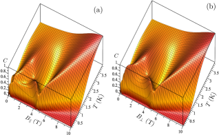
Figure 3: (a) Specific heat $C$ as a function of temperature and parallel external magnetic field. (b) Specific heat $C$ as a function of temperature and perpendicular external magnetic field. For the ${\rm Cu}_{3}-{\rm As}$ compound.

Figure 3a presents the specific heat as a function of temperature and the parallel external magnetic field $B_{\parallel}$. An anomalous behavior is noticeable at $B_{\parallel}\approx 4.5$ T, which manifests as an unusual peak in the low-temperature region. Additionally, two peculiar peaks appear at $B_{\parallel}\thicksim 2$ T, whereas other regions with a fixed magnetic field exhibit only one anomalous peak. Panel (b) illustrates an analogous plot, albeit with the perpendicular magnetic field $B_{\perp}$. The specific heat plots mainly resemble those in panel (a), with the exception of the absence of a minimum at $B_{\perp}\thicksim 2$ T. The low-temperature anomaly occurs at $B_{\parallel}\approx 5$ T. For a system with temperature around $T\sim 1$ K, the specific heat exhibits unusual behavior, absorbing or releasing heat more efficiently for a given temperature change. High specific heat is a beneficial property as it can enhance the overall efficiency and effectiveness of the triangular system. From the perspective of the MCE, this translates into more efficient magnetic cooling or heating.

III.4 Magnetization

We will now discuss magnetization, which has a key role in the MCE. The strength of the MCE is directly related to the change in magnetization of the compound in response to variation in temperature and the applied magnetic field. In our case, the magnetization can be derived without taking numerical derivatives, through the following relation

$$\left\langle\left(\tfrac{\partial\mathbf{H}}{\partial B_{k}}\right)\right\rangle=\frac{1}{Z}{\rm tr}\left\{\mathbf{H}_{B_{k}}{\rm e}^{-\mathbf{H}/T}\right\}=\frac{1}{Z}{\rm tr}\left\{\tilde{\mathbf{H}}_{B_{k}}{\rm e}^{-\mathbf{E}/T}\right\},$$ (9)

where $\tilde{\mathbf{H}}_{B_{k}}=\mathbf{U}\left(\tfrac{\partial\mathbf{H}}{\partial B_{k}}\right)\mathbf{U}^{-1}$, and $k=\{\|,\bot\}$. This method is a typical procedure to avoid numerical derivatives, as the Hamiltonian can be derived in relation to $B_{k}$ analytically. Therefore, the magnetization becomes

$$M_{k}=-\frac{1}{\mathfrak{g}_{k}}\left\langle\left(\tfrac{\partial\mathbf{H}}{\partial B_{k}}\right)\right\rangle,$$ (10)

where $\mathfrak{g}_{k}$ is a constant normalization chosen for convenience, defined as follows: $\mathfrak{g}_{k}=\frac{1}{3}\sum_{i=1}^{3}g_{i}^{k}$. The values of $\mathfrak{g}_{\parallel}$ is $2.25$ for both compounds, while the values of $\mathfrak{g}_{\perp}$ are $2.06$ and $2.07$ for As and Sb, respectively.

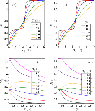
Figure 4: (a) Magnetization versus parallel magnetic field at various temperatures. (b) Magnetization versus perpendicular magnetic field at the same temperatures. (c) Temperature-dependent magnetization for different parallel magnetic fields for several parallel magnetic fields. (d) Analogously, temperature-dependent magnetization for a set of perpendicular magnetic fields. The study considers the ${\rm Cu}_{3}-{\rm As}$ compound.

Figure 4a presents the magnetization as a function of the parallel magnetic field, $B_{\parallel}$, at various temperature values, including zero-temperature. Note that a $1/3$ quasi-plateau feature appears, fading as temperature increases to around $1$K. Similarly, panel (b) reports magnetization as a function of a perpendicular external magnetic field. Here, the $1/3$ quasi-plateau becomes more noticeable, with effects largely mirroring those in the previous panel. Conversely, panel (c) displays magnetization as a function of temperature, considering multiple external magnetic fields parallel to the triangle plane. In this panel, the quasi-plateau region converges to $M\sim 0.5$, with a saturated region at $M\rightarrow 1.5$. A significant curvature change occurs at around $1$ K. Lastly, panel (d) illustrates the magnetization as a function of temperature for an external magnetic field perpendicular to the triangular plane. The magnetization behavior closely resembles that in panel (c), but with a more noticeable convergence to the $1/3$ quasi-plateau in low-temperature regions. Here again, the main curvature change happens approximately at $1$ K.

III.5 Magnetic Susceptibility

Magnetic susceptibility is another relevant quantity for studying the MCE as it determines how easily a material can be magnetized or demagnetized. To obtain this quantity, we can follow a procedure similar to the previous one. Thus the magnetic susceptibility, can be given by

$$\chi_{k}=\frac{1}{\mathfrak{g}_{k}^{2}T}\left\{\left\langle\left(\tfrac{\partial\mathbf{H}}{\partial B_{k}}\right)^{2}\right\rangle-\left\langle\left(\tfrac{\partial\mathbf{H}}{\partial B_{k}}\right)\right\rangle^{2}\right\}.$$ (11)

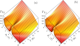
Figure 5: (a) Magnetic susceptibility times temperature, $T\chi_{\parallel}$ in the plane of temperature and parallel external magnetic field. (b) Magnetic susceptibility $T\chi_{\perp}$ in the plane of temperature and perpendicular external magnetic field.

Figure 5a illustrates the magnetic susceptibility times temperature ($T\chi_{\parallel}$) for ${\rm Cu}_{3}-{\rm As}$ compound, plotted against temperature (in kelvin) and parallel external magnetic field (tesla). It is noteworthy that at $B_{\parallel}\approx 4.5$ T, $T\chi_{\parallel}$ maintains a constant value of around $T\chi_{\parallel}\approx 0.3$. This means that the magnetic susceptibility inversely depends on the temperature in the low-temperature region. An alike finite value is observed for the null magnetic field. This is due to the shift from regions dominated by two aligned spins and one oppositely aligned spin, leading to complete alignment with the external magnetic field. The ${\rm Cu}_{3}-X$ compound, with higher magnetic susceptibility, can be magnetized or demagnetized more readily, resulting in greater thermal energy transfer and a more significant temperature change, roughly at $T\lesssim 1$ K. Similarly, panel (b) depicts the product of magnetic susceptibility and temperature, $T\chi_{\perp}$, in the plane of temperature and perpendicular external magnetic field. Although the behavior is quite similar to panel (a), there are slight differences, such as the pronounced change occurring at a slightly higher magnetic field, $B_{\perp}\approx 5$ T. Therefore, magnetic susceptibility affects the magnitude of the temperature change observed during the MCE and could play a crucial part in enhancing the magnetic refrigeration systems.

IV Magnetocaloric Effect

The Magnetocaloric Effect (MCE) refers to the thermal response of a material to the change in an external magnetic field. It holds potential for practical applications such as energy-efficient cooling technologies. Accordingly, we will discuss aspects like the isentropic curve and Grüneisen parameter.

IV.1 Isentropic curve

In magnetic systems, isentropic curves or adiabatic temperature curves provide a useful tool to visualize and understand the MCE. In the context of MCE, an isentropic curve represents a process that occurs at constant entropy in a magnetic field-temperature phase diagram.

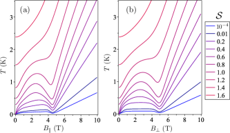
Figure 6: (a) Plot of isentropic $\mathcal{S}$ (in units of $k_{B})$ curve temperature $T\>({\rm K})$ against a parallel magnetic field $B_{\parallel}\;({\rm T})$. (b) Plot of isentropic curve temperature $T\>({\rm K})$ as a function of magnetic field $B_{\perp}\;({\rm T})$. Both plots are for the ${\rm Cu}_{3}-{\rm As}$ compound.

In Figure 6a, the isentropic curve for {${\rm Cu}_{3}-{\rm As}$} is illustrated for a parallel magnetic field. Between null magnetic field and $B_{\parallel}\approx 4.5$ T, the system exhibits the first step of magnetization, with two spins aligned parallel to the magnetic field while the third one is aligned antiparallel. Surely, for $B_{\parallel}\apprge 4.5$ T, all spins become aligned with the magnetic field. The isentropic curve shows high sensitivity at relatively low entropy, and as temperature increases, the crossover region between these two states manifests as a minimum. This minimum gradually disappears around $T\sim 1$ K. Notably, strong slopes of the isentropic curves occur around the minimum, indicating a large MCE in this region. Similarly, in Figure 6b, the isentropic curve for {${\rm Cu}_{3}-{\rm As}$} is depicted for a perpendicular magnetic field. The behavior of the isentropic curve is largely analogous to the previous case, with the only difference being that the minimum occurs at approximately $B_{\perp}\approx 5$ T. These curves provide insight into the temperature changes of a system in response to the application or removal of an external magnetic field. Additionally, the shape of the isentropic curve can provide valuable information about possible zero-temperature magnetic phase transitions in the {${\rm Cu}_{3}-{\rm As}$} compound.

IV.2 Grüneisen parameters

The Grüneisen parameter plays a essential role in understanding the MCE, which refers to the change in temperature of a material resulting from variations in an applied magnetic field. This effect has significant applications in magnetic cooling technologies. The Grüneisen parameter quantifies the relationship between the change in temperature of the compound and the magnetic field under constant entropy conditions. Specifically, the Grüneisen parameter $\Gamma$ is defined as the ratio of the temperature derivative of the magnetization per mole to the molar specific heat,

$$\Gamma_{k}=-\frac{1}{C}\!\left(\frac{\partial M}{\partial T}\right)_{B_{k}}\!=-\frac{\left(\tfrac{\partial\mathcal{S}}{\partial B_{k}}\right)_{T}}{T\left(\tfrac{\partial\mathcal{S}}{\partial T}\right)_{B_{k}}}=\frac{1}{T}\!\left(\frac{\partial T}{\partial B_{k}}\right)_{\mathcal{S}}\!,$$ (12)

To avoid numerical derivatives, an equivalent expression of the Grüneisen parameter can be derived

$$\Gamma_{k}=\frac{1}{\mathfrak{g}_{k}}\frac{\langle\mathbf{H}_{B_{k}}\mathbf{H}\rangle-\langle\mathbf{H}_{B_{k}}\rangle\langle\mathbf{H}\rangle}{\langle\mathbf{H}^{2}\rangle-\langle\mathbf{H}\rangle^{2}}.$$ (13)

Further research has explored these phenomena by analyzing the adiabatic temperature change, which demonstrates a strong correlation with the magnetic entropy change[37].

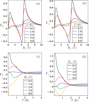
Figure 7: (a) Grüneisen parameter $\Gamma_{\parallel}$ as a function of parallel magnetic field $B_{\parallel}$, for a range of temperatures. (b) Grüneisen parameter $\Gamma_{\perp}$ as a function of perpendicular magnetic field. (c) $\Gamma_{\parallel}$ as a function of temperature for a set of parallel magnetic field. (d) $\Gamma_{\perp}$ as a function of temperature for a number of perpendicular magnetic field. The magnetic field is in units of tesla, while temperature is measured in kelvin. For the ${\rm Cu}_{3}-{\rm As}$ compound.

In Figure 7a, the Grüneisen parameter is illustrated as a function of the parallel magnetic field $B_{\parallel}$ for various fixed temperatures. The Grüneisen parameter shows significant changes in response to an applied magnetic field, with the most notable variations occurring at $B_{\parallel}\sim 1$ T for temperatures around $T\sim 1$ K. As the temperature increases, the magnitude of these changes decreases. Another region where the Grüneisen parameter becomes relevant is around $B_{\parallel}\approx 4.5$ T, exhibiting a strong variation. However, as the temperature increases, the magnitude of the Grüneisen parameter at this field strength decreases, eventually diminishing. Panel (b) presents an equivalent quantity obtained by applying a perpendicular magnetic field $B_{\perp}$, yielding results equivalent to the previous case. Additionally, in panel (c), we depict the variation of $\Gamma$ as a function of temperature for different external parallel magnetic fields. A significant change in the Grüneisen parameter $\Gamma_{\parallel}$ is observed for temperatures below $T\sim 2$ K. When the magnetic field is lower than $B_{\parallel}\sim 2$ T, $\Gamma_{\parallel}$ is positive, whereas for $B_{\parallel}\gtrsim 2$ T, this parameter becomes negative. Moreover, for temperatures $T\gtrsim 2$ K, the Grüneisen parameter decreases significantly. The final panel is similar to panel (c), but for a perpendicular magnetic field. Some differences arise, such as a stronger $\Gamma_{\perp}$ compared to the parallel case for low magnetic fields ($B_{\perp}\sim 0.5$ T) and the low-temperature region. Conversely, for large magnetic fields ($B_{\perp}\sim 4.0$ T), the Grüneisen parameter ($\Gamma_{\perp}$) is weaker than in the parallel case. In conclusion, the study of ${\rm Cu}_{3}-{\rm As}$ reveals a significant Grüneisen parameter at around $B\sim 5$ T, indicating a prominent MCE. This finding holds crucial implications for the selection and design of magnetic refrigeration systems.

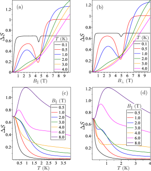
Figure 8: (a) Entropy variation $\Delta\mathcal{S}$ as a function of parallel magnetic field $B_{\parallel}$, for a set of fixed temperatures. (b) Entropy variation $\Delta\mathcal{S}$ as a function of perpendicular magnetic field. (c) $\Delta\mathcal{S}$ as a function of temperature for a variety of parallel magnetic field. (d)$\Delta\mathcal{S}$ as a function of temperature for different perpendicular magnetic fields.

Last but not least, the MCE can also be analyzed through the variation in entropy, $\Delta\mathcal{S}=\mathcal{S}(0,T)-\mathcal{S}(B,T)$, associated with the magnetic phase. This variation occurs due to the alignment or realignment of spins, resulting in changes in the disorder and order of the ${\rm Cu}_{3}-X$ compound and leading to a temperature change. Therefore, $\Delta\mathcal{S}$ is an important quantity to explore the magnetocaloric performance.

In Fig.8a, we illustrate $\Delta\mathcal{S}$ as a function of the parallel external magnetic field $B_{\parallel}$ for several fixed temperatures. We observe that at a temperature of $T\sim 0.1$ K, the entropy remains almost constant ($\Delta\mathcal{S}\sim\ln(2)\approx 0.7$). This is due to the system being roughly double degenerate at null magnetic field, and the degeneracy is broken by the presence of a magnetic field. There is a slight depression at $T\approx 4.5$ K, indicating a change in the dominant phases at this magnetic field. This behavior changes significantly as the temperature increases. For $B_{\parallel}\lesssim 4.5$ T, $\Delta\mathcal{S}$ decreases significantly, while for $B_{\parallel}\gtrsim 4.5$ T, it becomes larger. Panel (b) shows an analogous behavior but for the perpendicular external magnetic field $B_{\perp}$. The only difference is that the depression occurs at $B_{\perp}\lesssim 5.0$T. Furthermore, in panel (c), we present $\Delta\mathcal{S}$ as a function of temperature for several fixed parallel magnetic fields $B_{\parallel}$. For magnetic fields below $B_{\parallel}\lesssim 4.5$ T, $\Delta\mathcal{S}$ decreases monotonically. However, for stronger magnetic fields $B_{\parallel}\gtrsim 4.5$ T, a maximum appears, indicating a peak in $\Delta\mathcal{S}$. Similarly, panel (d) depicts $\Delta\mathcal{S}$ as a function of temperature, assuming a fixed perpendicular magnetic field. The behavior is mainly similar to panel (c), although $\Delta\mathcal{S}$ does not decrease monotonically. Additionally, for strong magnetic fields, it also exhibits a maximum, as observed in the previous panel.

V Conclusions

In this paper, we conduct a theoretical exploration of the ${\rm Cu}_{3}-X$ antiferromagnetic spin system (where $\mathrm{X=As,Sb}$), which is identified by its isosceles or slightly distorted equilateral triangular configurations, as detailed in reference [21, 23, 24]. This system can be accurately depicted using the Heisenberg model on a triangular structure, incorporating factors like the exchange interaction, Dzyaloshinskii-Moriya interaction, g-factors, and external magnetic fields.

Recently, ${\rm Cu}_{3}-X$ has garnered significant attention due to its fundamental properties [21, 23, 24]. Furthermore, the scientific community has shown a growing interest in the exploration of several magnetic compounds [25, 26, 27, 28, 29, 30, 31] due to their diverse potential in areas such as spintronics, nanotechnology, and biomedicine.

Our investigation uses a numerical approach to analyze both zero-temperature and finite-temperature behaviors of the ${\rm Cu}_{3}$-like spin system. At zero temperature, the system exhibits twofold degenerate energy in the absence of a magnetic field and a $1/3$ quasi-plateau magnetization when the magnetic field is varied. At finite temperatures, our focus primarily lies on analyzing magnetic properties such as magnetization, magnetic susceptibility, entropy, and specific heat.

In addition, we examine the MCE in relation to an externally applied magnetic field, oriented both parallel and perpendicular to the plane of the triangular structure. The ${\rm Cu}_{3}-X$ displays remarkably consistent behavior for both orientations of the magnetic field. We also extend our study to include the evaluation of the isentropic curve, the Grüneisen parameter, and the variation in entropy during the application or removal of the magnetic field. Therefore, in the low temperature region below $T\sim 1$K and for approximately 4.5T and 5T for parallel and perpendicular magnetic fields, respectively, our results confirm that the MCE is more prominent in this region. This study could contribute to the research and development of nano-compounds with triangular structures, potentially improving the performance of the Magnetocaloric Effect (MCE). Such advancements may be especially intriguing for applications in the cryogenic temperature range that utilize moderate magnetic fields.

- [1] O. Tegus, E. Brück, K, H. J. Buschow, F. R. de Boer, Transition-metal-based magnetic refrigerants for room-temperature applications, Nature 415, 150 (2002).
- [2] T. Gruner, D. Kim, M. Brando, A. V. Dukhnenko, N. Y. Shitsevalova, V. B. Filipov, D. Jang, Reversible and irreversible magnetocaloric effect: The cases of rare-earth intermetallics YbPt2Sn and , Jour. Magn. Mag. Mat., 489, 165389 (2019)
- [3] K. A. Gschneidner Jr, V. K. Pecharsky, A. O. Tsokol, Recent developments in magnetocaloric materials, Rep. Prog. Phys. 68 1479 (2005).
- [4] J. Liu, T. Gottschall, K. P. Skokov, J. D. Moore, O. Gutfleisch, Giant magnetocaloric effect driven by structural transitions, Nature Mat. 11, 620 (2012).
- [5] J. Darby, J. Hatton, B. V. Rollin, E. F. W. Seymour and H. B. Silsbee, Experiments on the Production of Very Low Temperatures by Two-Stage Demagnetization, Proceedings Phys. Soc. A, 64, 861 (1951)
- [6] G. V. Brown, Magnetic heat pumping near room temperature, Jour. Appl. Phys., 47, 3673 (1976)
- [7] V. K. Pecharsky, K. A. Gschneidner Jr., Giant Magnetocaloric Effect in , Phys. Rev. Lett., 78, 4494 (1997).
- [8] C. Zimm, A. Jastrab, A. Sternberg, V. K. Pecharsky, K. A. Gschneidner Jr., M. Osborne, I. Anderson, Description and Performance of a Near-Room Temperature Magnetic Refrigerator, Adv. Cryog. Eng., 43, 1759 (1998).
- [9] V. K. Pecharsky, K. A. Gschneidner Jr., A. O. Pecharsky, A. M. Tishin, Thermodynamics of the magnetocaloric effect, Phys. Rev. B, 64, 144406 (2001).
- [10] D.N. Ba, L. Becerra, N. Casaretto, J.E. Duvauchelle, M. Marangolo, S. Ahmim, M. Almanza, M. LoBue, Magnetocaloric Gadolinium thick films for energy harvesting applications, AIP Adv. 10, 035110 (2020).
- [11] D.N. Ba, Y.L. Zheng, L. Becerra, M. Marangolo, M. Almanza, M. LoBue, Magnetocaloric effect in flexible, free-standing gadolinium thick films for energy conversion applications, Phys. Rev. Appl. 15, 064045 (2021)
- [12] F. Zhang, C. Taake, B. Huang, X. You, H. Ojiyed, Q. Shen, I. Dugulan, L. Caron, N. van Dijk, E. Brücka, Magnetocaloric effect in the system: From bulk to nano, Acta Materialia 224, 117532 (2022)
- [13] K. Klinar, M.M. Rojo, Z. Kutnjak, A. Kitanovski, Toward a solid-state thermal diode for room-temperature magnetocaloric energy conversion, J. Appl. Phys. 127, 234101 (2020)
- [14] V. Chaudhary, Z. Wang, A. Ray, I. Sridhar, R.V. Ramanujan, Self pumping magnetic cooling, J. Phys. D 50, 03LT03 (2017)
- [15] M.S. Pattanaik, S.K. Cheekati, V.B. Varma, R.V. Ramanujan, App. Therm. Eng. 201, 117777 (2022)
- [16] U. Sen, S. Chatterjee, S, Sen, M. K. Tiwari, A. Mukhopadhyay, R. Ganguly, A novel magnetic cooling device for long distance heat transfer, J. Magn. Magn. Mater. 421, 165 (2017)
- [17] M. Qian, X. Zhang, L. Wei, P. Martin, J. Sun, L. Geng, T. B. Scott, H.-X. Peng, Tunable magnetocaloric effect in Ni-Mn-Ga microwires, Scientific Reports 8, 16574 (2018)
- [18] X.L. Liu, Y.F. Zhang, Y.Y. Wang, W.J. Zhu, G.L. Li, X.W. Ma, Y.H. Zhang, S.Z. Chen, S. Tiwari, K.J. Shi, S.W. Zhang, H.M. Fan, Y.X. Zhao, X.J. Liang, Comprehensive understanding of magnetic hyperthermia for improving antitumor therapeutic efficacy, Theranostics 10, 3793 (2020)
- [19] J.B. Li, Y. Qu, J. Ren, W.Z. Yuan, D.L. Shi, Magnetocaloric effect in magnetothermally-responsive nanocarriers for hyperthermia-triggered drug release, Nanotechnology 23, 505706 (2012)
- [20] T. Yamase, E. Ishikawa, K. Fukaya, H. Nojiri, T. Taniguchi, and T. Atake, Spin-frustrated -triangle-sandwiching octadecatungstates as a new class of molecular magnets, Inorg. Chem. 43, 8150 (2004)
- [21] K-Y Choi, Y. H. Matsuda and H. Nojiri, Observation of a Half Step Magnetization in the -Type Triangular Spin Ring, Phys. Rev. Lett. 96, 107202 (2006)
- [22] M. Trif, F. Troiani, D. Stepanenko, and D. Loss, Spin-Electric Coupling in Molecular Magnets, Rev. Lett. 101, 217201 (2008)
- [23] K-Y Choi, N. S. Dalal, A. P. Reyes, P.L. Kuhns, Y. H. Matsuda , H. Hojiri, S. S. Mal and U. Kortz, Pulsed-field magnetization, electron spin resonance, and nuclear spin-lattice relaxation in the spin triangle, Phys. Rev. B 77, 024406 (2008)
- [24] K.-Y. Choi, Z. Wang, H. Nojiri, J. van Tol, P. Kumar, P. Lemmens, B. S. Bassil, U. Kortz, and N. S. Dalal, Coherent Manipulation of Electron Spins in the Spin Triangle Complex Impregnated in Nanoporous Silicon, Phys. Rev. Lett. 108, 067206 (2012)
- [25] M.-A. Bouammali, N. Suaud, N. Guihéry, and R. Maurice, Antisymmetric Exchange in a Real Copper Triangular Complex, Inorg. Chem. 61, 12138 (2022)
- [26] E. T. Spielberg, A. Gilb, D. Plaul, D. Geibig, D. Hornig, D. Schuch, A. Buchholz, A. Ardavan, and W. Plass, A Spin-Frustrated Trinuclear Copper Complex Based on Triaminoguanidine with an Energetically Well-Separated Degenerate Ground State, Inorg. Chem. 54, 3432 (2015)
- [27] M. I. Belinsky, Spin Chirality of Cu3 and V3 Nanomagnets. 2. Frustration, Temperature, and Distortion Dependence of Spin Chiralities and Magnetization in the Rotating and Tilted Magnetic Fields, Inorg. Chem. 55, 4091 (2016)
- [28] J. Robert, N. Parizel, P. Turek, A. K. Boudalis, Relevance of Dzyaloshinskii–Moriya spectral broadenings in promoting spin decoherence: a comparative pulsed-EPR study of two structurally related iron(iii) and chromium(iii) spin-triangle molecular qubits, Phys. Chem. Phys. 21, 19575 (2019)
- [29] A. K. Boudalis, Half-Integer Spin Triangles: Old Dogs, New Tricks, Chem. Eur. J. 27, 7022 (2021)
- [30] A. C. Stowe, S. Nellutla, N. S. Dalal, U. Kortz, Magnetic Properties of Lone-Pair-Containing, Sandwich-Type Polyoxoanions: A Detailed Study of the Heteroatomic Effect, Eur. J. Inorg. Chem. 2004, 3792 (2004)
- [31] U. Kortz, S. Nellutla, A. C. Stowe, N. S. Dalal, J. van Tol, B. S. Bassil, Structure and Magnetism of the Tetra-Copper(II)-Substituted Heteropolyanion , Inorg. Chem. 43, 144 (2004)
- [32] P. Kowalewska, K. Szałowski, Magnetocaloric properties of V6 molecular magnet, J. Magn. Magn. Mater. 496, 165933 (2020)
- [33] K. KarǏová, J. Strečka, J. Richter, Enhanced magnetocaloric effect in the proximity of magnetization steps and jumps of spin-1/2 XXZ Heisenberg regular polyhedra, J. Phys.: Condens. Matter 29, 125802 (2017)
- [34] J. Torrico and J. A. Plascak, Ground state and thermodynamic properties of spin-1/2 isosceles Heisenberg triangles for -like magnetic molecules, Phys. Rev. E 102, 062116 (2020)
- [35] J. Torrico and J. A. Plascak, Study of the ground state and thermodynamic properties of Cu5-NIPA-like molecular nanomagnets, J. Magn. Magn. Mater. 552, 169151 (2022)
- [36] P. J. von Ranke, W. S. Torres, Theoretical investigation of crystalline electric field influence on the magnetocaloric effect in the cubic praseodymium system , Phys. Rev. B 105, 085153 (2022)
- [37] L. Zhu, M. Garst, A. Rosch, and Q. Si, Universally Diverging Grüneisen Parameter and the Magnetocaloric Effect Close to Quantum Critical Points, Phys. Rev. Lett. 91, 066404 (2003)