Bayesian Cramér-Rao Bound Estimation with Score-Based Models

Abstract

The Bayesian Cramér-Rao bound (CRB) provides a lower bound on the error of any Bayesian estimator under mild regularity conditions. It can be used to benchmark the performance of estimators, and provides a principled design metric for guiding system design and optimization. However, the Bayesian CRB depends on the prior distribution, which is often unknown for many problems of interest. This work develops a new data-driven estimator for the Bayesian CRB using score matching, a statistical estimation technique, to model the prior distribution. The performance of the estimator is analyzed in both the classical parametric modeling regime and the neural network modeling regime. In both settings, we develop novel non-asymptotic bounds on the score matching error and our Bayesian CRB estimator. Our proofs build on results from empirical process theory, including classical bounds and recently introduced techniques for characterizing neural networks, to address the challenges of bounding the score matching error. The performance of the estimator is illustrated empirically on a denoising problem example with a Gaussian mixture prior.

I Introduction

The Bayesian Cramér-Rao bound (CRB) [1], also known as the posterior or Van Trees CRB, provides a lower bound on the error covariance in Bayesian inference. Originally introduced by Van Trees, it is the Bayesian analog of the classical CRB and is widely used to guide system design and benchmark the performance of estimators. It has found a number of applications, including image registration [2, 3], dynamic system analysis [4], and communication array design [5].

Analytic computation of the Bayesian CRB requires knowledge of the Stein score (i.e., the derivative of the log-density) of the prior distribution and likelihood function. While for many applications of interest (e.g., medical imaging [6] and communication [7] systems), the likelihood function can be determined from physical principles, the prior distribution is often more complex and difficult to model. For example, in various inverse problems in imaging (e.g., image deconvolution or tomographic imaging), it has long been an open problem to model the probability distribution for certain image classes of interest. While generic or hand-crafted priors (e.g., [8, 9]) can be adopted, this could lead to substantial error in the Bayesian CRB calculation due to oversimplification and misspecification of the prior distribution. Motivated by these challenges and the ever-increasing availability of large data sets [10], the goal of this paper is to develop a provably accurate estimator of the Bayesian CRB when the likelihood function is known but only samples are available to characterize the prior distribution.

I-A Estimation of Cramér-Rao Type Bounds

Existing estimators of Cramér-Rao type bounds generally focus on the classical CRB and its inverse, the Fisher information. These estimators can be broadly split into two categories: plug-in approaches that first estimate the likelihood function and form the CRB using this estimate, and direct approaches that estimate the CRB without first estimating the likelihood [11].

Plug-in approaches can use parametric or non-parametric estimators of the likelihood. An example of a non-parametric approach can be found in [12], which uses density estimation using field theory (DEFT) [13] to estimate the underlying distribution. The authors demonstrate that this approach yields good performance on a univariate Gaussian distribution. However, the work does not provide any theoretical guarantees, and the approach does not scale well to high dimensions due to the curse of dimensionality inherent to DEFT.

A parametric plug-in approach was recently introduced by Habi et al [14, 15]. The main idea behind their approach is the use of a conditional normalizing flow to model the likelihood function. The authors demonstrate experimentally that this approach is accurate for Gaussian and non-Gaussian measurement models and can provide useful information for image denoising and image edge detection tasks. They also provide non-asymptotic bounds on the estimator error. However, their bounds rely on strong assumptions (e.g., the score of the likelihood function is required to be bounded, which does not hold for many widely used likelihood functions such as Gaussians), and the bounds depend on the total variation distance between the learned generative model and the true measurement distribution, which is unknown.

Direct approaches for CRB estimation exploit the relationship between $f$-divergences and the Fisher information [16, 11]. Specifically, these approaches require first estimating the $f$-divergence between the original likelihood function and a perturbed version of the likelihood for different choices of perturbations. Here the $f$-divergence can be estimated using the Friedman-Rafskay (FR) multivariate test statistic [16] or a neural network based mutual information estimator [11]. A semi-definite program is then solved to estimate the Fisher information from the $f$-divergence estimates. In [11], it was shown that these approaches can also be used for Bayesian CRB estimation.

While the above direct approaches are attractive because they avoid the estimation of the infinite-dimensional density function required by plug-in methods, they come with several practical difficulties. Specifically, both approaches require the estimation of the $f$-divergence for at least $D(D+1)/2$ perturbations where $D$ is the dimension of the unknown parameters, which is computationally expensive in high dimensions and, in the case of [11], requires the optimization of a separate neural network for each choice of perturbation. The approaches also do not have provable convergence guarantees.

I-B Our Contributions

Inspired by recent advances in generative modeling, this work introduces a novel Bayesian CRB estimator with non-asymptotic convergence guarantees. The key idea behind our approach is to use score matching [17] to directly estimate the score of the unknown prior distribution. Score matching is a statistical score estimation technique that minimizes the distance between the scores of the data and model distribution. Compared with plug-in approaches that use density estimation techniques such as maximum likelihood estimation, score matching has the advantage of being independent of the model’s normalizing constant, which is often intractable. It is also a key component of diffusion models, which have achieved state-of-the-art results in generative modeling [18].

To characterize the convergence properties of our estimator, we consider two different modeling regimes. The first regime corresponds to a classical parametric modeling setting where the number of model parameters is less than the number of prior samples. The second regime considers the case where the score model is a neural network. In both regimes, the key difficulty is establishing bounds on the score matching error, which is challenging because the score model is vector valued and the score matching objective depends on the Jacobian of the model. To address this challenge, we develop novel non-asymptotic score matching bounds in both regimes. Our proofs are based on several results from empirical process theory, including the rate theorem [19], Talagrand’s inequality for empirical processes [20], and neural network covering bounds [21]. To the best of our knowledge, this work is the first to provide non-asymptotic bounds on score matching with general neural network models.

The performance of our proposed estimator was validated in an empirical study of a ten-dimensional denoising problem with a synthetic Gaussian mixture prior. The results demonstrate the accuracy of our estimator at a wide range of signal-to-noise ratio (SNR) levels.

I-C Organization

The remainder of this paper is organized as follows. Section II introduces notation and provides technical background on the Bayesian CRB and score matching. Section III formally introduces the problem formulation and our estimator. Section IV then provides our convergence results in the classical setting, while Section V derives the bounds in the neural network setting. Results from the numerical experiments are presented in Section VI. Finally, Section VII provides concluding remarks and a discussion of future research directions.

II Background and Preliminaries

II-A Notation

We use bold letters to denote vectors (e.g., $\mathbf{x}$) and capital bold letters to denote matrices and higher-order tensors (e.g., $\mathbf{X}$). The gradient of a scalar-valued function $f(\mathbf{x}):\mathbb{R}^{N}\to\mathbb{R}$ is denoted $\nabla_{\mathbf{x}}f(\mathbf{x})$ and is written as an $N\times 1$ vector. The Jacobian of a vector-valued function $F(\mathbf{x}):\mathbb{R}^{N}\to\mathbb{R}^{M}$ is written as an $M\times N$ matrix, denoted $\nabla_{\mathbf{x}}F(\mathbf{x})$, with $[\nabla_{\mathbf{x}}F(\mathbf{x})]_{i,j}=\partial F(\mathbf{x})_{i}/\partial\mathbf{x}_{j}$. We use $\mathbf{x}_{1}^{N}$ as shorthand for the data set $\{\mathbf{x}_{1},\cdots,\mathbf{x}_{N}\}$.

We use $\mathbf{X}^{T}$, $\text{tr}(\mathbf{X})$, $\mathbf{X}^{-1}$, and $\mathbf{X}^{\dagger}$ to respectively denote the transpose, trace, inverse, and Moore-Penrose pseudoinverse of a given matrix $\mathbf{X}$. For square matrices $\mathbf{A}$ and $\mathbf{B}$, the generalized inequality $\mathbf{A}\succcurlyeq\mathbf{B}$ means that $\mathbf{A}-\mathbf{B}$ is a positive semidefinite matrix. We use $\|\cdot\|_{\sigma}$ to denote the spectral norm of a given matrix, while $\|\cdot\|_{2}$ is used to denote the component-wise two-norm of a given tensor; thus, for a matrix, it corresponds to the Frobenius norm. The expression $\|\cdot\|_{p,q}$ denotes the $(p,q)$ matrix norm, defined by $\|\mathbf{X}\|_{p,q}=\|[\|\mathbf{X}_{:,1}\|_{p},\cdots,\|\mathbf{X}_{:,M}\|_{p}]^{T}\|_{q}$ for $\mathbf{X}\in\mathbb{R}^{N\times M}$. The bilinear expression $\langle\cdot,\cdot\rangle$ refers to the standard Euclidean inner product.

For random vectors $\mathbf{x}$ and $\mathbf{y}$, we use $p(\mathbf{x})$ to denote the density function of $\mathbf{x}$, $p(\mathbf{y}|\mathbf{x})$ to denote the conditional density of $\mathbf{y}$ given $\mathbf{x}$, and $p(\mathbf{x},\mathbf{y})$ to denote the joint density function. The term $\mathbb{E}_{\mathbf{x}}$ denotes the expectation with respect to $\mathbf{x}$, $\mathbb{E}_{\mathbf{x},\mathbf{y}}$ denotes the expectation with respect to the joint distribution of $\mathbf{x}$ and $\mathbf{y}$, and $\mathbb{E}_{\mathbf{y}|\mathbf{x}}$ denotes the conditional expectation of $\mathbf{y}$ given $\mathbf{x}$. The $\epsilon$-covering number of a set $A$ with respect to a given norm $d$ is denoted $N(A,d,\epsilon)$. We use $\log(\cdot)$ to refer to the natural logarithm.

II-B The Bayesian CRB

Let $\mathbf{x}\in\mathcal{X}\subset\mathbb{R}^{D}$ be a random parameter vector of interest, let $\mathbf{y}\in\mathcal{Y}\subset\mathbb{R}^{K}$ be observations from a model with parameters $\mathbf{x}$, and let $\hat{\mathbf{x}}(\mathbf{y})$ be an estimator of $\mathbf{x}$. Assume the following regularity conditions hold.

Assumption II.1 (Support).

The set $\mathcal{X}$ is either $\mathbb{R}^{D}$ or an open bounded subset of $\mathbb{R}^{D}$ with piecewise smooth boundary.

Assumption II.2 (Existence of Derivatives).

The derivatives $[\nabla_{\mathbf{x}}p(\mathbf{x},\mathbf{y})]_{i}$, $i=1,\dots,D$, exist and are absolutely integrable.

Assumption II.3 (Finite Expected Error).

The expected error for the estimator as a function of $\mathbf{x}$, i.e., $B(\mathbf{x})\triangleq\int\left(\hat{\mathbf{x}}(\mathbf{y})-\mathbf{x}\right)p(\mathbf{y}\mid\mathbf{\mathbf{x}})\;d\mathbf{y}$, exists and is finite for all $\mathbf{x}$.

Assumption II.4 (Positive Density).

The joint probability density is nonzero for all $\mathbf{x},\mathbf{y}$.

Assumption II.5 (Dominated Convergence).

The probability function $p(\mathbf{x},\mathbf{y})$ and estimator $\hat{\mathbf{x}}(\mathbf{y})$ satisfy

$$\nabla_{\mathbf{x}}\int p(\mathbf{x},\mathbf{y})\left[\hat{\mathbf{x}}(\mathbf{y})-\mathbf{x}\right]^{T}d\mathbf{y}=\int\nabla_{\mathbf{x}}\left(p(\mathbf{x},\mathbf{y})[\hat{\mathbf{x}}(\mathbf{y})-\mathbf{x}]^{T}\right)d\mathbf{y}$$

for all $\mathbf{x}$.

Assumption II.6 (Error Boundary Conditions).

Let $\partial\mathcal{X}$ denote the boundary of $\mathcal{X}$. For any sequence $\{\mathbf{x}_{i}\}_{i=0}^{\infty}$, $\mathbf{x}_{i}\in\mathcal{X}$, such that $\mathbf{x}_{i}\to\mathbf{x}\in\partial\mathcal{X}$, we have that $B(\mathbf{x}_{i})p(\mathbf{x}_{i})\to 0$.

Under the above assumptions, the Bayesian CRB can be defined via information inequality [1]:

$$\mathbb{E}_{\mathbf{x},\mathbf{y}}\left[\left(\hat{\mathbf{x}}(\mathbf{y})-\mathbf{x}\right)(\hat{\mathbf{x}}\left(\mathbf{y})-\mathbf{x}\right)^{T}\right]\succcurlyeq\mathbf{V}_{B}\triangleq\mathbf{J}_{B}^{-1}.$$

Here $\mathbf{V}_{B}\in\mathbb{R}^{D\times D}$ denotes the Bayesian CRB and $\mathbf{J}_{B}\in\mathbb{R}^{D\times D}$ is the Bayesian information, which can be written as

$$\mathbf{J}_{B}\triangleq\mathbb{E}_{\mathbf{x},\mathbf{y}}\left[\nabla_{\mathbf{x}}\log p(\mathbf{x},\mathbf{y})\nabla_{\mathbf{x}}\log p(\mathbf{x},\mathbf{y})^{T}\right].$$

The Bayesian information can be decomposed into a prior-informed term $\mathbf{J}_{P}$ and a data-informed term $\mathbf{J}_{D}$, i.e., [1]:

$$\mathbf{J}_{B}=\mathbf{J}_{P}+\mathbf{J}_{D}.$$ (1)

Here $\mathbf{J}_{P}$ is defined as

$$\mathbf{J}_{P}\triangleq\mathbb{E}_{\mathbf{x}}\left[\nabla_{\mathbf{x}}\log p(\mathbf{x})\nabla_{\mathbf{x}}\log p(\mathbf{x})^{T}\right],$$

while $\mathbf{J}_{D}$ is the average Fisher information associated with the observations, i.e.,

$$\mathbf{J}_{D}\triangleq\mathbb{E}_{\mathbf{x},\mathbf{y}}\left[\nabla_{\mathbf{x}}\log p(\mathbf{y}|\mathbf{x})\nabla_{\mathbf{x}}\log p(\mathbf{y}|\mathbf{x})^{T}\right]=\mathbb{E}_{\mathbf{x}}\left[\mathbf{J}_{F}(\mathbf{x})\right],$$

where

$$\mathbf{J}_{F}(\mathbf{x})\triangleq\mathbb{E}_{\mathbf{y}|\mathbf{x}}\left[\nabla_{\mathbf{x}}\log p(\mathbf{y}|\mathbf{x})\nabla_{\mathbf{x}}\log p(\mathbf{y}|\mathbf{x})^{T}\right]$$

is the Fisher information.

II-C Score Matching

Score matching [17] is a statistical method for estimating the (Stein) score of an unknown data distribution $p(\mathbf{x})$, i.e., $\nabla_{\mathbf{x}}\log p(\mathbf{x})$, from a set of i.i.d. samples $\{\mathbf{x}_{1},\mathbf{x}_{2},\cdots,\mathbf{x}_{N}\}\subset\mathbb{R}^{D}$. Originally introduced by Hvärinen and Dayan, the technique is based on minimizing the Fisher divergence between the data scores and the scores of a vector-valued model $s(\mathbf{x};\boldsymbol{\theta}):\mathbb{R}^{D}\to\mathbb{R}^{D}$ parameterized by $\boldsymbol{\theta}\in\boldsymbol{\Theta}$:

$$L(\boldsymbol{\theta})\triangleq\frac{1}{2}\mathbb{E}_{\mathbf{x}}\left[\|s(\mathbf{x};\boldsymbol{\theta})-\nabla_{\mathbf{x}}\log p(\mathbf{x})\|_{2}^{2}\right].$$ (2)

Minimizing (2) directly is intractable since $\nabla_{\mathbf{x}}\log p(\mathbf{x})$ is unknown. However, under the following regularity conditions, Hvärinen and Dayan proved that $L(\boldsymbol{\theta})=J(\boldsymbol{\theta})+C$, where $C$ is a constant independent of $\boldsymbol{\theta}$ and

$$J(\boldsymbol{\theta})\triangleq\mathbb{E}_{\mathbf{x}}\left[\text{tr}\left(\nabla_{\mathbf{x}}s(\mathbf{x};\boldsymbol{\theta})\right)+\frac{1}{2}\|s(\mathbf{x};\boldsymbol{\theta})\|_{2}^{2}\right].$$ (3)

Assumption II.7 (Regularity of Score Functions).

The score function estimate $s(\mathbf{x};\boldsymbol{\theta})$ and the true score function $\nabla_{\mathbf{x}}\log p(\mathbf{x})$ are both differentiable with respect to $\mathbf{x}$. They additionally satisfy $\mathbb{E}_{\mathbf{x}}\left[\|s(\mathbf{x},\boldsymbol{\theta})\|_{2}^{2}\right]<\infty$ for all $\boldsymbol{\theta}\in\boldsymbol{\Theta}$ and $\mathbb{E}_{\mathbf{x}}\left[\nabla_{\mathbf{x}}\|\log p(\mathbf{x})\|_{2}^{2}\right]<\infty$.

Assumption II.8 (Score Matching Boundary Conditions).

For any $\boldsymbol{\theta}\in\boldsymbol{\Theta}$ and any sequence $\{\mathbf{x}_{i}\}_{i=0}^{\infty}$, $\mathbf{x}_{i}\in\mathcal{X}$, such that $\mathbf{x}_{i}\to\mathbf{x}\in\partial\mathcal{X}$, we have that $s(\mathbf{x}_{i};\boldsymbol{\theta})p(\mathbf{x}_{i})\to\mathbf{0}$ for all $\boldsymbol{\theta}\in\boldsymbol{\Theta}$.

The proof is based on integration by parts [17]. The following unbiased estimator of (3) is then obtained with the samples $\mathbf{x}_{1}^{N}$:

$$\hat{J}(\boldsymbol{\theta};\mathbf{x}_{1}^{N})\triangleq\frac{1}{N}\sum_{i=1}^{N}\text{tr}\left(\nabla_{\mathbf{x}}s(\mathbf{x}_{i};\boldsymbol{\theta})\right)+\frac{1}{2}\|s(\mathbf{x}_{i};\boldsymbol{\theta})\|_{2}^{2}.$$ (4)

Note that computing (4) only requires the evaluation of the vector-valued model and its derivative, and under additional regularity conditions, (4) is a consistent estimator of (3) [17, 22].

Since the introduction of score matching, a number of extensions and variants of the technique have been developed. Hvärinen extended the approach to binary-valued variables and variables defined over bounded domains [23]. Kingma and LeCun introduced a regularized version of score matching [24]. Song et al developed a scalable version of score matching, known as sliced score matching, for high-dimensional data by using projections to approximate the Jacobian term in the score matching objective [22]. They also showed that their approach was consistent, and that both the original and sliced score matching objectives lead to asymptotically normal estimators of the score. Song and Ermon’s seminal generative modeling work [25] then leveraged both sliced score matching and a denoising version of score matching introduced by Vincent [26] as training objectives for diffusion models, which have achieved state-of-the-art results in generative modeling [18].

Theoretical results in the works cited above are limited to asymptotic characterizations of score matching. To the best of our knowledge, the only previous non-asymptotic bounds on score matching were developed by Koehler et al in [27], which considers the case where score matching is used to learn an energy-based model, i.e., a deep generative model parameterized up to the constant of parameterization. Koehler et al show that in this setting the expected Kullback–Leibler (KL) divergence between the data distribution and the learned distribution can be bounded by a term proportional to the Rademacher complexity of the parameterized model class and the log-Sobolev constant, which relates the KL divergence to the score matching loss. This approach provides important insight into score matching performance. However, it does not attempt to bound the Rademacher complexity, and can therefore be viewed as somewhat orthogonal to our score matching analysis, which provides explicit error bounds.

III Proposed Estimator

Given i.i.d. samples $\{\mathbf{x}_{1},\mathbf{x}_{2},\cdots,\mathbf{x}_{N}\}\subset\mathbb{R}^{D}$ from a prior distribution $p(\mathbf{x})$ and a known likelihood function $p(\mathbf{y}|\mathbf{x})$, our task is to obtain an estimate $\hat{\mathbf{V}}_{B}(\mathbf{x}_{1}^{N})$ of the Bayesian CRB $\mathbf{V}_{B}$. Here we have assumed Assumptions II.1 - II.6 hold to make the problem well-defined. This problem is well motivated from a variety of applications (e.g., imaging or communications) in which we have complete knowledge of the measurement process (e.g., from physics), in addition to our prior information through some previously collected training data.

To address the problem, we propose a data-driven estimator of the Bayesian CRB using score matching. The proposed method makes use of the decomposition of $\mathbf{J}_{B}$ in (1), and estimates $\mathbf{J}_{P}$ and $\mathbf{J}_{D}$ separately. To estimate $\mathbf{J}_{P}$, we use the following estimator:

$$\hat{\mathbf{J}}_{P}(\mathbf{x}_{1}^{N})=\frac{1}{N}\sum_{i=1}^{N}s(\mathbf{x}_{i};\hat{\boldsymbol{\theta}}_{N})s(\mathbf{x}_{i};\hat{\boldsymbol{\theta}}_{N})^{T},$$ (5)

where $s(\mathbf{x}_{i};\hat{\boldsymbol{\theta}}_{N})$ is the prior score estimate obtained by minimizing the empirical score matching loss (4), and we have assumed Assumptions II.7 and II.8 hold. Note that in (5), we use the sample mean to approximate the expectation.

To estimate $\mathbf{J}_{D}$, we consider the following two cases for the known data model. First, if $\mathbf{J}_{F}(\mathbf{x})$ can be computed analytically with the given data model (e.g., a linear/nonlinear Gaussian or Poisson model), we use the following estimator:

$$\hat{\mathbf{J}}_{D}(\mathbf{x}_{1}^{N})=\frac{1}{N}\sum_{i=1}^{N}\mathbf{J}_{F}(\mathbf{x}_{i}).$$ (6)

Note that this encompasses a linear Gaussian model as a special example, in which $\mathbf{J}_{F}(\mathbf{x})$ is a constant independent of $\mathbf{x}$. Second, if $\mathbf{J}_{F}(\mathbf{x})$ cannot be computed in a closed-form, we construct the following estimator:

$$\hat{\mathbf{J}}_{D}(\mathbf{x}_{1}^{N})=\frac{1}{N}\sum_{i=1}^{N}\hat{\mathbf{J}}_{F}(\mathbf{x}_{i}),$$ (7)

where

$$\hat{\mathbf{J}}_{F}(\mathbf{x}_{i})=\frac{1}{M}\sum_{j=1}^{M}\nabla_{\mathbf{x}}\log p(\mathbf{y}_{j}^{i}\,|\,\mathbf{x}_{i})\nabla_{\mathbf{x}}\log p(\mathbf{y}_{j}^{i}\,|\,\mathbf{x}_{i})^{T}.$$

Here we assume that we can obtain i.i.d. samples from the given data model (e.g., using Monte Carlo methods [28]), i.e., $\mathbf{y}_{j}^{i}\sim p(\mathbf{y}\,|\,\mathbf{x}_{i})$ for $j=1,\cdots,M$.

Putting together the above estimators for $\mathbf{J}_{P}$ and $\mathbf{J}_{D}$, we form the following estimator for the Bayesian information:

$$\hat{\mathbf{J}}_{B}(\mathbf{x}_{1}^{N})=\hat{\mathbf{J}}_{P}(\mathbf{x}_{1}^{N})+\hat{\mathbf{J}}_{D}(\mathbf{x}_{1}^{N}),$$

from which we obtain the Bayesian CRB estimator:

$$\hat{\mathbf{V}}_{B}(\mathbf{x}_{1}^{N})=\hat{\mathbf{J}}_{B}(\mathbf{x}_{1}^{N})^{\dagger},$$

where the pseudoinversion ensures that $\hat{\mathbf{V}}_{B}(\mathbf{x}_{1}^{N})$ is well defined.

IV Convergence in the Classical Regime

The goal of this section is to derive non-asymptotic error bounds for our Bayesian information and Bayesian CRB estimators in the classical parametric regime, where the dimension of the score model parameter space is less than the number of available samples from the prior distribution. To this end, we first obtain a generalization bound on the distance between the minimizer of the empirical score matching loss $\hat{\boldsymbol{\theta}}_{N}$ and the true minimizer $\boldsymbol{\theta}^{*}\triangleq\operatorname*{arg\,min}_{\boldsymbol{\theta}\in\boldsymbol{\Theta}}L(\boldsymbol{\theta})$ by leveraging existing score matching bounds and the rate theorem from empirical process theory [19]. We then build off of this result and covariance matrix estimation bounds [29] to obtain error bounds for the Bayesian CRB estimator.

IV-A Score Matching Convergence Rate

In this subsection, we provide convergence rate analysis for score matching, which we will use to prove error bounds for our Bayesian information and Bayesian CRB estimators. We first summarize key results from previous work on the consistency of the score matching estimator [17, 22]. As in [22], we require the following three assumptions to hold.

Assumption IV.1 (Compactness).

The parameter space $\boldsymbol{\Theta}$ is compact.

Assumption IV.2 (Lipschitz Continuity).

Both $\nabla_{\mathbf{x}}s(\mathbf{x};\boldsymbol{\theta})$ and $s(\mathbf{x};\boldsymbol{\theta})s(\mathbf{x};\boldsymbol{\theta})^{T}$ are Lipschitz continuous in terms of the Frobenius norm, i.e., for any $\boldsymbol{\theta}_{1},\boldsymbol{\theta}_{2}\in\boldsymbol{\Theta}$, $\|\nabla_{\mathbf{x}}s(\mathbf{x};\boldsymbol{\theta}_{1})-\nabla_{\mathbf{x}}s(\mathbf{x};\boldsymbol{\theta}_{2})\|_{2}\leq L_{1}(\mathbf{x})\|\boldsymbol{\theta}_{1}-\boldsymbol{\theta}_{2}\|_{2}$ and $\|s(\mathbf{x};\boldsymbol{\theta}_{1})s(\mathbf{x};\boldsymbol{\theta}_{1})^{T}-s(\mathbf{x};\boldsymbol{\theta}_{2})s(\mathbf{x};\boldsymbol{\theta}_{2})^{T}\|_{2}\leq L_{2}(\mathbf{x})\|\boldsymbol{\theta}_{1}-\boldsymbol{\theta}_{2}\|_{2}$. Additionally, we require $\mathbb{E}_{\mathbf{x}}[L_{1}(\mathbf{x})^{2}]<\infty$ and $\mathbb{E}_{\mathbf{x}}[L_{2}(\mathbf{x})^{2}]<\infty$.

Assumption IV.3 (Exact Minimization).

The optimized parameters $\hat{\boldsymbol{\theta}}_{N}$ exactly minimize the empirical loss (4).

From these assumptions, we obtain the following uniform bound on the expected error from the empirical approximation of the true score matching objective. The theorem is a straightforward modification of Lemma 3 in [22], which proves a similar bound for sliced score matching.

Theorem 1 (Uniform convergence of the expected error).

Assume the score matching regularity conditions (Assumptions II.7 and II.8) hold and Assumptions IV.1 and IV.2 are satisfied. Then there exists a constant $C_{S}$ such that

$$\mathbb{E}_{\mathbf{x}}\left[\sup_{\boldsymbol{\theta}\in\boldsymbol{\Theta}}\left|\hat{J}(\boldsymbol{\theta};\mathbf{x}_{1}^{N})-J(\boldsymbol{\theta})\right|\right]\leq\frac{C_{S}}{\sqrt{N}}$$ (8)

for all $N$.

Proof Sketch.

We first show that $\ell(\mathbf{x};\boldsymbol{\theta})\triangleq\text{tr}\left(\nabla_{\mathbf{x}}s(\mathbf{x};\boldsymbol{\theta})\right)+\frac{1}{2}\|s(\mathbf{x};\boldsymbol{\theta})\|_{2}^{2}$ is Lipschitz continuous in $\boldsymbol{\theta}$ (Lemma 10), which is an analogous result to Lemma 2 in [22]). Uniform convergence of the expected error then follows using standard techniques from empirical process theory (i.e., the symmetrization trick and Dudley’s entropy integral). See Appendix A for the full proof. ∎

In this work, we also require the following additional assumption, which ensures that the objective function is well behaved around $\boldsymbol{\theta}^{*}$.

Assumption IV.4 (Locally Quadratic).

There exist $\lambda,\eta>0$ such that

$$J(\boldsymbol{\theta})\geq J(\boldsymbol{\theta}^{*})+\lambda\|\boldsymbol{\theta}-\boldsymbol{\theta}^{*}\|_{2}^{2}$$

for all $\boldsymbol{\theta}\in B_{\eta}(\boldsymbol{\theta}^{*})$. Further, we have that

$$J(\boldsymbol{\theta})\geq J(\boldsymbol{\theta}^{*})+\lambda\eta^{2}$$

for all $\boldsymbol{\theta}\not\in B_{\eta}(\boldsymbol{\theta}^{*})$.

Using the above assumption, we can bound the score matching error in parameter space.

Lemma 1.

Assume the score matching regularity conditions (Assumptions II.7 and II.8) hold and Assumptions IV.1, IV.2, and IV.3 are satisfied. Then

$$\mathbb{P}\left[\|\hat{\boldsymbol{\theta}}_{N}-\boldsymbol{\theta}^{*}\|_{2}\geq\eta\right]\leq\frac{2C_{S}}{\sqrt{N}\lambda\eta^{2}}.$$ (9)

Proof.

We have that

$$\mathbb{E}_{\mathbf{x}}\left[J(\hat{\boldsymbol{\theta}}_{N})-J(\boldsymbol{\theta}^{*})\right] =\mathbb{E}_{\mathbf{x}}\left[\hat{J}(\hat{\boldsymbol{\theta}}_{N};\mathbf{x}_{1}^{N})+(J(\hat{\boldsymbol{\theta}}_{N})-\hat{J}(\hat{\boldsymbol{\theta}}_{N};\mathbf{x}_{1}^{N}))-\hat{J}(\boldsymbol{\theta}^{*};\mathbf{x}_{1}^{N})-(J(\boldsymbol{\theta}^{*})-\hat{J}(\boldsymbol{\theta}^{*};\mathbf{x}_{1}^{N}))\right]$$

$$\stackrel{{\scriptstyle\footnotesize\mathclap{\mbox{$(i)$}}}}{{\leq}}\mathbb{E}_{\mathbf{x}}\left[(J(\hat{\boldsymbol{\theta}}_{N})-\hat{J}(\hat{\boldsymbol{\theta}}_{N};\mathbf{x}_{1}^{N}))-(J(\hat{\boldsymbol{\theta}}_{N})-\hat{J}(\hat{\boldsymbol{\theta}}_{N};\mathbf{x}_{1}^{N})\right]$$

$$\leq\mathbb{E}_{\mathbf{x}}\left[|J(\hat{\boldsymbol{\theta}}_{N})-\hat{J}(\hat{\boldsymbol{\theta}}_{N};\mathbf{x}_{1}^{N})|\right]+\mathbb{E}_{\mathbf{x}}\left[|J(\boldsymbol{\theta}^{*})-\hat{J}(\boldsymbol{\theta}^{*};\mathbf{x}_{1}^{N})|\right]$$

$$\stackrel{{\scriptstyle\footnotesize\mathclap{\mbox{$(ii)$}}}}{{\leq}}2\frac{C_{S}}{\sqrt{N}},$$

where $(i)$ holds since $\hat{J}(\hat{\boldsymbol{\theta}}_{N};\mathbf{x}_{1}^{N})\leq\hat{J}(\boldsymbol{\theta}^{*};\mathbf{x}_{1}^{N})$ by definition of $\hat{\boldsymbol{\theta}}_{N}$ and $(ii)$ is by Theorem 1. Applying Markov’s inequality gives

$$\mathbb{P}\left[J(\hat{\boldsymbol{\theta}}_{N})-J(\boldsymbol{\theta}^{*})\geq\lambda\eta^{2}\right]\leq\frac{2C_{S}}{\sqrt{N}\lambda\eta^{2}}.$$

By Assumption IV.4, this implies that

$$\mathbb{P}\left[\|\hat{\boldsymbol{\theta}}_{N}-\boldsymbol{\theta}^{*}\|_{2}\geq\eta\right]\leq\frac{2C_{S}}{\sqrt{N}\lambda\eta^{2}}$$

as desired. ∎

After a change of variables, (9) can be rewritten as

$$\mathbb{P}\left[\|\hat{\boldsymbol{\theta}}_{N}-\boldsymbol{\theta}^{*}\|_{2}\geq\frac{\sqrt{2C_{S}}}{\sqrt{\lambda\epsilon}N^{1/4}}\right]\leq\epsilon,$$

so the convergence rate has $N^{1/4}$ dependence on $N$. In the following, we show that this rate can be improved upon. Our proof utilizes the following corollary of Theorem 1.

Corollary 1.

Assume all of the previously stated assumptions hold. Then there exists a $C_{\boldsymbol{\theta}}>0$ such that for any $\delta>0$,

$$\mathbb{E}_{\mathbf{x}}\left[\sup_{\|\boldsymbol{\theta}-\boldsymbol{\theta}^{*}\|_{2}\leq\delta}\left|\Delta_{N}(\boldsymbol{\theta})\right|\right]\leq\frac{C_{\boldsymbol{\theta}}\sqrt{P}\delta}{\sqrt{N}}$$

for all $N$, where $P$ is the dimension of the parameter space $\boldsymbol{\Theta}$, $C_{\boldsymbol{\theta}}$ is independent of $P$, and

$$\Delta_{N}(\boldsymbol{\theta})\triangleq(\hat{J}(\boldsymbol{\theta};\mathbf{x}_{1}^{N})-J(\boldsymbol{\theta}))-(\hat{J}(\boldsymbol{\theta}^{*};\mathbf{x}_{1}^{N})-J(\boldsymbol{\theta}^{*})).$$

Proof.

See Appendix A. ∎

We are now ready to present our score matching convergence rate result. The proof is based on the rate of convergence theorem for empirical processes [19, Theorem 3.2.5].

Theorem 2.

Assume all of the previously stated assumptions hold. Then for any $\epsilon>0$ and all $N\geq N^{\prime}\triangleq 16C_{S}^{2}/\epsilon^{2}\lambda^{2}\eta^{4}$, with probability at least $1-\epsilon$ it holds that

$$\sqrt{N}\lVert\hat{\boldsymbol{\theta}}_{N}-\boldsymbol{\theta}^{*}\rVert_{2}\leq\frac{8C_{\boldsymbol{\theta}}\sqrt{P}}{\epsilon\lambda}.$$

Proof.

See Appendix A.

∎

IV-B Bayesian CRB Bounds

In this subsection we prove non-asymptotic error bounds on the proposed estimators of the Bayesian information and Bayesian CRB using the just-proved score matching convergence rate. Our result requires an additional assumption, which ensures the scores of the prior distribution and likelihood function are well-behaved.

Assumption IV.5 (Sub-Gaussian Scores).

The random vectors $\nabla_{\mathbf{x}}\log p(\mathbf{x})$ and $\nabla_{\mathbf{x}}\log p(\mathbf{y}\,|\,\mathbf{x})$ are sub-Gaussian with norms $C_{P}$ and $C_{D}$, respectively, i.e., for any $\mathbf{z}\in\mathbb{S}^{D-1}$ we have that

$$\mathbb{E}_{\mathbf{x}}\left[e^{\langle\nabla_{\mathbf{x}}\log p(\mathbf{x}),\mathbf{z}\rangle^{2}/C_{P}^{2}}\right]\leq 2$$

and

$$\mathbb{E}_{\mathbf{x},\mathbf{y}}\left[e^{\langle\nabla_{\mathbf{x}}\log p(\mathbf{y}\mid\mathbf{x}),\mathbf{z}\rangle^{2}/C_{D}^{2}}\right]\leq 2.$$

Note that this assumption is satisfied for many Bayesian models of interest, such as those with Gaussian or Gaussian mixture priors and likelihood functions. The following example shows this is the case for a model with a Gaussian prior.

Example 1 (Gaussian prior).

Consider a model with a Gaussian prior and without loss of generality assume that the prior is zero mean. Letting $\boldsymbol{\Sigma}$ denote its covariance matrix, for any $\mathbf{z}\in\mathbb{S}^{D-1}$ we have that

$$\mathbb{E}_{\mathbf{x}}\left[e^{\langle\nabla_{\mathbf{x}}\log p(\mathbf{x}),\mathbf{z}\rangle^{2}/C_{P}^{2}}\right] =\mathbb{E}_{\mathbf{x}}\left[e^{\langle-\boldsymbol{\Sigma}^{-1}\mathbf{x},\mathbf{z}\rangle^{2}/C_{P}^{2}}\right]$$

$$=C\int_{\mathbf{x}}e^{-\frac{1}{2}\mathbf{x}^{T}\boldsymbol{\Sigma}^{-1}\mathbf{x}}e^{\langle-\boldsymbol{\Sigma}^{-1}\mathbf{x},\mathbf{z}\rangle^{2}/C_{P}^{2}}\;d\mathbf{x}$$

$$\leq C\int_{\mathbf{x}}e^{-\frac{1}{2}\mathbf{x}^{T}\boldsymbol{\Sigma}^{-1}\mathbf{x}}e^{\mathbf{x}^{T}\boldsymbol{\Sigma}^{-2}\mathbf{x}/C_{P}^{2}}\;d\mathbf{x}.$$

where $C$ is the normalizing constant for the Gaussian prior and the inequality holds because $\mathbf{z}\in\mathbb{S}^{D-1}$. Setting $C_{P}$ so that $C_{P}^{2}=2\|\boldsymbol{\Sigma}^{-1}\|_{2}\beta$, $\beta>1$, we have that

$$C\int_{\mathbf{x}}e^{-\frac{1}{2}\mathbf{x}^{T}\boldsymbol{\Sigma}^{-1}\mathbf{x}}e^{\mathbf{x}^{T}\boldsymbol{\Sigma}^{-2}\mathbf{x}/C_{P}^{2}}\;d\mathbf{x}\leq C\int_{\mathbf{x}}e^{-\frac{1}{2}\mathbf{x}^{T}\boldsymbol{\Sigma}^{-1}\mathbf{x}}e^{\mathbf{x}^{T}\boldsymbol{\Sigma}^{-1}\mathbf{x}/(2\beta)}\;d\mathbf{x}=C\int_{\mathbf{x}}e^{-\frac{\beta-1}{2\beta}\mathbf{x}^{T}\boldsymbol{\Sigma}^{-1}\mathbf{x}}\;d\mathbf{x},$$

which is clearly finite. Further scaling $C_{P}$ so that the integral is less than $2$ shows that $\nabla_{\mathbf{x}}\log p(\mathbf{x})$ is sub-Gaussian. So Gaussian priors satisfy Assumption IV.5.

In addition to the above assumption, our results make use of the following two lemmas.

Lemma 2.

Let $\mathbf{x}\in\mathbb{R}^{D}$ be a sub-Gaussian random vector, and define

$$\hat{\boldsymbol{\Sigma}}\triangleq\frac{1}{N}\sum_{i=1}^{N}\mathbf{x}_{i}\mathbf{x}_{i}^{T},\quad\boldsymbol{\Sigma}\triangleq\mathbb{E}_{\mathbf{x}}\left[\mathbf{x}\mathbf{x}^{T}\right].$$

Then for all $\epsilon>0$, with probability at least $1-\epsilon$ we have

$$\lVert\hat{\boldsymbol{\Sigma}}-\boldsymbol{\Sigma}\rVert_{2}\leq C_{\boldsymbol{\Sigma}}\|\mathbf{x}\|^{2}_{\psi_{2}}m\left(\sqrt{\frac{D-\log(\epsilon)}{N}}\right),$$

where $\|\cdot\|_{\psi_{2}}$ is the sub-Gaussian norm, $C_{\boldsymbol{\Sigma}}$ is a universal constant, and $m(t)\triangleq\mathrm{max}\{t,t^{2}\}$.

Proof.

This is a minor modification of [30, Proposition 2.1]. ∎

Lemma 3.

Assume all of the previously stated assumptions hold. Then

$$\mathbb{E}_{\mathbf{x}}\left[\|s(\mathbf{x};\boldsymbol{\theta}^{*})s(\mathbf{x};\boldsymbol{\theta}^{*})^{T}-\nabla_{\mathbf{x}}\log p(\mathbf{x})\nabla_{\mathbf{x}}\log p(\mathbf{x})^{T}\|_{\sigma}\right]\leq 2L(\boldsymbol{\theta}^{*})+2\mu_{P}\sqrt{2L(\boldsymbol{\theta}^{*})},$$ (10)

where $\mu_{P}\triangleq\mathbb{E}_{\mathbf{x}}\left[\|\nabla_{\mathbf{x}}\log p(\mathbf{x})\|_{2}^{2}\right]^{1/2}$.

Proof.

We have that

$$\mathbb{E}_{\mathbf{x}} \left[\|s(\mathbf{x};\boldsymbol{\theta}^{*})s(\mathbf{x};\boldsymbol{\theta}^{*})^{T}-\nabla_{\mathbf{x}}\log p(\mathbf{x})\nabla_{\mathbf{x}}\log p(\mathbf{x})^{T}\|_{\sigma}\right]$$

$$\hskip 28.45274pt=\mathbb{E}_{\mathbf{x}}\left[\|s(\mathbf{x};\boldsymbol{\theta}^{*})s(\mathbf{x};\boldsymbol{\theta}^{*})^{T}-s(\mathbf{x};\boldsymbol{\theta}^{*})\nabla_{\mathbf{x}}\log p(\mathbf{x})^{T}+s(\mathbf{x};\boldsymbol{\theta}^{*})\nabla_{\mathbf{x}}\log p(\mathbf{x})^{T}-\nabla_{\mathbf{x}}\log p(\mathbf{x})\nabla_{\mathbf{x}}\log p(\mathbf{x})^{T}\|_{\sigma}\right]$$

$$\hskip 28.45274pt\leq\mathbb{E}_{\mathbf{x}}\left[\|s(\mathbf{x};\boldsymbol{\theta}^{*})\left(s(\mathbf{x};\boldsymbol{\theta}^{*})-\nabla_{\mathbf{x}}\log p(\mathbf{x})\right)^{T}\|_{\sigma}\right]+\mathbb{E}_{\mathbf{x}}\left[\|\left(s(\mathbf{x};\boldsymbol{\theta}^{*})-\nabla_{\mathbf{x}}\log p(\mathbf{x})\right)\nabla_{\mathbf{x}}\log p(\mathbf{x})^{T}\|_{\sigma}\right]$$

$$\hskip 28.45274pt=\mathbb{E}_{\mathbf{x}}\left[\|\left(s(\mathbf{x};\boldsymbol{\theta}^{*})-\nabla_{\mathbf{x}}\log p(\mathbf{x})+\nabla_{\mathbf{x}}\log p(\mathbf{x})\right)\left(s(\mathbf{x};\boldsymbol{\theta}^{*})-\nabla_{\mathbf{x}}\log p(\mathbf{x})\right)^{T}\|_{\sigma}\right]$$

$$\hskip 28.45274pt\quad\quad+\mathbb{E}_{\mathbf{x}}\left[\|\left(s(\mathbf{x};\boldsymbol{\theta}^{*})-\nabla_{\mathbf{x}}\log p(\mathbf{x})\right)\nabla_{\mathbf{x}}\log p(\mathbf{x})^{T}\|_{\sigma}\right]$$

$$\hskip 28.45274pt\leq\mathbb{E}_{\mathbf{x}}\left[\|\left(s(\mathbf{x};\boldsymbol{\theta}^{*})-\nabla_{\mathbf{x}}\log p(\mathbf{x})\right)\left(s(\mathbf{x};\boldsymbol{\theta}^{*})-\nabla_{\mathbf{x}}\log p(\mathbf{x})\right)^{T}\|_{\sigma}\right]$$

$$\hskip 28.45274pt\quad\quad+2\mathbb{E}_{\mathbf{x}}\left[\|\left(s(\mathbf{x};\boldsymbol{\theta}^{*})-\nabla_{\mathbf{x}}\log p(\mathbf{x})\right)\nabla_{\mathbf{x}}\log p(\mathbf{x})^{T}\|_{\sigma}\right]$$

$$\hskip 28.45274pt\stackrel{{\scriptstyle\footnotesize\mathclap{\mbox{$(i)$}}}}{{\leq}}\mathbb{E}_{\mathbf{x}}\left[\|s(\mathbf{x};\boldsymbol{\theta}^{*})-\nabla_{\mathbf{x}}\log p(\mathbf{x})\|_{2}^{2}\right]+2\mathbb{E}_{\mathbf{x}}\left[\|s(\mathbf{x};\boldsymbol{\theta}^{*})-\nabla_{\mathbf{x}}\log p(\mathbf{x})\|_{2}\|\nabla_{\mathbf{x}}\log p(\mathbf{x})\|_{2}\right],$$ (11)

where $(i)$ holds by sub-multiplicity of the matrix norm. Now note that since $\mathbf{J}_{P}$ is well defined and $\mu_{P}=\sqrt{\text{tr}(\mathbf{J}_{P})}$, $\mu_{P}$ is also well defined. We can therefore apply the Cauchy–Schwarz inequality to (IV-B) to obtain

$$\mathbb{E}_{\mathbf{x}} \left[\|s(\mathbf{x};\boldsymbol{\theta}^{*})s(\mathbf{x};\boldsymbol{\theta}^{*})^{T}-\nabla_{\mathbf{x}}\log p(\mathbf{x})\nabla_{\mathbf{x}}\log p(\mathbf{x})^{T}\|_{\sigma}\right]$$

$$\hskip 28.45274pt\leq\mathbb{E}_{\mathbf{x}}\left[\|s(\mathbf{x};\boldsymbol{\theta}^{*})-\nabla_{\mathbf{x}}\log p(\mathbf{x})\|_{2}^{2}\right]+2\mathbb{E}_{\mathbf{x}}\left[\|\nabla_{\mathbf{x}}\log p(\mathbf{x})\|_{2}^{2}\right]^{1/2}\mathbb{E}_{\mathbf{x}}\left[\|s(\mathbf{x};\boldsymbol{\theta}^{*})-\nabla_{\mathbf{x}}\log p(\mathbf{x})\|_{2}^{2}\right]^{1/2}$$

$$\hskip 28.45274pt=2L(\boldsymbol{\theta}^{*})+2\mu_{P}\sqrt{2L(\boldsymbol{\theta}^{*})},$$

as desired. ∎

We now introduce the main results of this section.

Theorem 3.

Assume all of the previously stated assumptions hold. Then for any $\epsilon>0$ and any $N\geq N^{\prime}$, the Bayesian information estimator satisfies, with probability at least $1-\epsilon$,

$$\|\hat{\mathbf{J}}_{B}(\mathbf{x}_{1}^{N})-\mathbf{J}_{B}\|_{\sigma}\leq C_{1}\left[(C_{P}^{2}+C_{D}^{2})\mathrm{m}\left(\sqrt{\frac{D-\log(\epsilon)}{N}}\right)+\frac{C_{\boldsymbol{\theta}}\sqrt{P}}{\epsilon\lambda\sqrt{N}}\left(\mu_{L}+\frac{\sigma_{L}}{\sqrt{\epsilon N}}\right)+\frac{1}{\epsilon}\left(L(\boldsymbol{\theta}^{*})+\mu_{P}\sqrt{L(\boldsymbol{\theta}^{*})}\right)\right],$$ (12)

where $C_{1}$ is a universal constant, $\mu_{L}\triangleq\mathbb{E}_{\mathbf{x}}\left[L_{2}(\mathbf{x})\right]$, and $\sigma_{L}^{2}\triangleq\mathbb{E}_{\mathbf{x}}\left[(L_{2}(\mathbf{x})-\mu_{L})^{2}\right]$.

Proof Sketch.

Through application of the triangle inequality, the Bayesian information estimation error can be bounded by the error in sample-based estimation of $\mathbf{J}_{D}$ and $\mathbf{J}_{P}$, a model mismatch term, and error in the score estimates. The sample based estimation error terms can be handled using Lemma 2, the model mismatch terms can be handled using Lemma 3 and Markov’s inequality, and the score matching error term can be bounded using Theorem 2. See Appendix A for a full proof. ∎

Remark 1.

A bound on the Bayesian information estimation error can still be proven if Assumption IV.5 is weakened. For example, if the score vectors are sub-exponential, a weaker version of Theorem 3 can be proven using covariance estimation bounds for sub-exponential random variables (see, e.g., [30]).

Theorem 4.

Assume all of the previously stated assumptions hold and that the model is well-specified, i.e., $L(\boldsymbol{\theta}^{*})=0$. Then there exists a constant $C_{V}$ such that for any $\epsilon>0$ and any $N\geq C_{V}\mathrm{max}\{D-\log(\epsilon),1/\epsilon^{2}\}$, the Bayesian CRB estimator satisfies, with probability at least $1-\epsilon$,

$$\|\hat{\mathbf{V}}_{B}(\mathbf{x}_{1}^{N})-\mathbf{V}_{B}\|_{\sigma}\leq C_{2}\|\mathbf{V}_{B}\|_{\sigma}^{2}\left[(C_{P}^{2}+C_{D}^{2})\mathrm{m}\left(\sqrt{\frac{D-\log(\epsilon)}{N}}\right)+\frac{C_{\boldsymbol{\theta}}\sqrt{P}}{\epsilon\lambda\sqrt{N}}\left(\mu_{L}+\frac{\sigma_{L}}{\sqrt{\epsilon N}}\right)\right],$$ (13)

where $C_{2}$ is a universal constant.

Proof.

Assume that $\hat{\mathbf{J}}_{B}(\mathbf{x}_{1}^{N})$ is invertible, which will be guaranteed later by concentration arguments. Conditioned on this event, $\hat{\mathbf{V}}_{B}(\mathbf{x}_{1}^{N})-\mathbf{V}_{B}$ can be rewritten as

$$\hat{\mathbf{V}}_{B}(\mathbf{x}_{1}^{N})-\mathbf{V}_{B} =\hat{\mathbf{V}}_{B}(\mathbf{x}_{1}^{N})(\mathbf{J}_{B}-\hat{\mathbf{J}}_{B}(\mathbf{x}_{1}^{N}))\mathbf{V}_{B}$$

$$=(\hat{\mathbf{V}}_{B}(\mathbf{x}_{1}^{N})-\mathbf{V}_{B}+\mathbf{V}_{B})(\mathbf{J}_{B}-\hat{\mathbf{J}}_{B}(\mathbf{x}_{1}^{N}))\mathbf{V}_{B}$$

$$=(\hat{\mathbf{V}}_{B}(\mathbf{x}_{1}^{N})-\mathbf{V}_{B})(\mathbf{J}_{B}-\hat{\mathbf{J}}_{B}(\mathbf{x}_{1}^{N}))\mathbf{V}_{B}+\mathbf{V}_{B}(\mathbf{J}_{B}-\hat{\mathbf{J}}_{B}(\mathbf{x}_{1}^{N}))\mathbf{V}_{B}.$$

Let $\Delta\triangleq\mathbf{J}_{B}-\hat{\mathbf{J}}_{B}(\mathbf{x}_{1}^{N})$. Taking the norm of both sides of the above expression and applying the triangle inequality gives

$$\|\hat{\mathbf{V}}_{B}(\mathbf{x}_{1}^{N})-\mathbf{V}_{B}\|_{\sigma}\leq\|\hat{\mathbf{V}}_{B}(\mathbf{x}_{1}^{N})-\mathbf{V}_{B}\|_{\sigma}\|\Delta\|_{\sigma}\|\mathbf{V}_{B}\|_{\sigma}+\|\mathbf{V}_{B}\|_{\sigma}^{2}\|\Delta\|_{\sigma},$$

which can be rewritten as

$$\|\hat{\mathbf{V}}_{B}(\mathbf{x}_{1}^{N})-\mathbf{V}_{B}\|_{\sigma}(1-\|\Delta\|_{\sigma}\|\mathbf{V}_{B}\|_{\sigma})\leq\|\mathbf{V}_{B}\|_{\sigma}^{2}\|\Delta\|_{\sigma}.$$

Note that by Theorem 3 and the well-specified assumption, for $N\geq C_{V}\mathrm{max}\{D-\log(\epsilon),1/\epsilon^{2}\}$, $C_{V}\geq 16C_{S}^{2}/\lambda^{2}\eta^{4}$, it holds that

$$\|\Delta\|_{\sigma}\leq C_{1}\left[(C_{P}^{2}+C_{D}^{2})\sqrt{\frac{1}{C_{V}}}+\frac{C_{\boldsymbol{\theta}}\sqrt{P}}{\lambda\sqrt{C_{V}}}\left(\mu_{L}+\frac{\sigma_{L}}{\sqrt{C_{V}}}\right)\right].$$

with probability at least $1-\epsilon$. So we can choose $C_{V}$ such $\|\Delta\|_{\sigma}\leq 1/2\|\mathbf{V}_{B}\|_{\sigma}$ with probability at least $1-\epsilon$. In this regime $\hat{\mathbf{J}}_{B}(\mathbf{x}_{1}^{N})$ is guaranteed to be invertible, and it holds that

$$\|\hat{\mathbf{V}}_{B}(\mathbf{x}_{1}^{N})-\mathbf{V}_{B}\|_{\sigma} \leq(1-\|\Delta\|_{\sigma}\|\mathbf{V}_{B}\|_{\sigma})^{-1}\|\mathbf{V}_{B}\|_{\sigma}^{2}\|\Delta\|_{\sigma}$$

$$\leq 2\|\mathbf{V}_{B}\|_{\sigma}^{2}\|\Delta\|_{\sigma}.$$

Applying Theorem 3 with $L(\boldsymbol{\theta}^{*})=0$ to $\Delta$, taking the union bound of the above probabilities, and introducing the universal constant gives the desired result. ∎

Remark 2.

The above theorems establish non-asymptotic bounds for our Bayesian information and CRB estimators. These results rely on a couple of key assumptions, including a locally quadratic objective function (Assumption IV.4) and sub-Gaussian score vectors (Assumption IV.5). However, the consistency of our estimators, i.e., their asymptotic convergence, can be proven without these assumptions. See our early work for the theorem and proof [31].

V Convergence with Neural Network Models

The Bayesian information and Bayesian CRB bounds in the previous section have $\sqrt{P}$ dependence on the dimension $P$ of the parameter space $\boldsymbol{\Theta}$ and $1/{\sqrt{N}}$ dependence on the sample size $N$. Since modern neural networks are often highly overparameterized, i.e., $N\ll P$, these bounds are inadequate for cases where the score model is a neural network. In this section, we address this limitation by developing bounds for our estimator with neural network score models that have improved dependence on the parameter space dimension. Specifically, we make the following assumption about the form of $s(\mathbf{x};\boldsymbol{\theta})$.

Assumption V.1 (Model Structure).

The parametric model $s(\mathbf{x};\boldsymbol{\theta})$ is a feedforward neural network that can be written as follows:

$$s(\mathbf{x};\boldsymbol{\theta})=\sigma_{L}(\mathbf{W}_{L}\sigma_{L-1}(\cdots\sigma_{1}(\mathbf{W}_{1}\mathbf{x}))).$$

Here $\boldsymbol{\theta}\triangleq\{\mathbf{W}_{i}\}_{i=1}^{L}$ are the neural network weights, i.e., $\mathbf{W}_{i}\in\mathbb{R}^{d_{i}\times d_{i-1}}$ with $d_{0}=d_{L}=D$. The $\{\sigma_{i}\}_{i=1}^{L}$ are fixed nonlinearities $\sigma_{i}:\mathbb{R}^{d_{i}}\to\mathbb{R}^{d_{i}}$. We assume that they satisfy the following properties:

1. They are Lipschitz with Lipschitz constants $\{\rho_{i}\}^{L}_{i=1}$.

2. They satisfy $\sigma_{i}(0)=0$.

3. Evaluation of the derivatives of the is $\tau_{i}$-Lipschitz i.e.,

   $$\left\lVert\,\nabla_{\mathbf{x}}\sigma_{i}(\mathbf{x})|_{\mathbf{s}}-\nabla_{\mathbf{x}}\sigma_{i}(\mathbf{x})|_{\mathbf{t}}\,\right\rVert_{2}\leq\tau_{i}\|\mathbf{s}-\mathbf{t}\|_{2}$$

   for any $\mathbf{s},\mathbf{t}\in\mathbb{R}^{d_{i}}$.

4. The Jacobians are bounded by constants $f_{i}$ in the spectral norm, i.e., $\|\,\nabla_{\mathbf{x}}\sigma_{i}(\mathbf{x})|_{\mathbf{s}}\,\|_{\sigma}\leq f_{i}$ for any $\mathbf{s}\in\mathbb{R}^{d_{i}}$.

Note that many commonly used nonlinearities, such as pointwise Tanh or Softplus functions, satisfy the above conditions. We also make two additional assumptions about the model and data distribution.

Assumption V.2 (Bounded Support).

The data distribution has bounded support, i.e., there exists a constant $T$ such that $\|\mathbf{x}\|_{2}\leq T$ for all $\mathbf{x}\in\mathcal{X}$.

Assumption V.3 (Bounded Weights).

The model weights $\mathbf{W}_{i}$ lie in spaces $\mathcal{W}_{i}$ that satisfy $\|\mathbf{W}_{i}\|_{\sigma}\leq c_{i}$ and $\|\mathbf{W}_{i}\|_{2,1}\leq b_{i}$ for all $\mathbf{W}_{i}\in\mathcal{W}_{i}$ and all $i$. The parameter space $\boldsymbol{\Theta}$ therefore denotes the Cartesian product space $\mathcal{W}_{1}\times\mathcal{W}_{2}\times\dots\times\mathcal{W}_{L}$.

Finally, as in Section IV, we make an assumption regarding the optimized model parameters.

Assumption V.4 (Neural Network Optimization).

The optimized parameters $\hat{\boldsymbol{\theta}}_{N}$ satisfy $\hat{J}(\hat{\boldsymbol{\theta}}_{N};\mathbf{x}_{1}^{N})\leq\hat{J}(\boldsymbol{\theta}^{*};\mathbf{x}_{1}^{N})$.

V-A Score Matching Convergence Rate

This subsection provides a bound on $L(\hat{\boldsymbol{\theta}}_{N})$, the score matching error, under the above assumptions. To that end, we first show that $L(\hat{\boldsymbol{\theta}}_{N})$ can be related to the empirical Rademacher complexity of the neural network function class. Our result makes use of the following two lemmas.

Lemma 4 (Theorem 2.1 in [20]).

Let $\mathcal{F}$ be a class of functions that maps $\mathcal{X}$ into $[-M,M]$. Assume that there is some $r\geq 0$ such that for every $f\in\mathcal{F}$, $\mathrm{var}[f(\mathbf{x})]\leq r$. Then for every $\epsilon>0$, with probability at least $1-\epsilon$ over the data $\mathbf{X}=[\mathbf{x}_{1},\ldots,\mathbf{x}_{N}]$, we have that

$$\sup_{f\in\mathcal{F}}\mathbb{E}_{\mathbf{x}}f(\mathbf{x})-\frac{1}{N}\sum_{i=1}^{N}f(\mathbf{x}_{i})\leq 6\mathfrak{R}\left(\mathcal{F}|_{\mathbf{X}}\right)+\sqrt{\frac{2r\log(2/\epsilon)}{N}}+\frac{32M\log(2/\epsilon)}{3N},$$

where $\mathcal{F}|_{\mathbf{X}}\triangleq\{[f(\mathbf{x}_{1}),\dots,f(\mathbf{x}_{N})]\mid f\in\mathcal{F}\}$ and $\mathfrak{R}\left(\mathcal{F}|_{\mathbf{X}}\right)$ is the empirical Rademacher complexity of $\mathcal{F}$, i.e.,

$$\mathfrak{R}\left(\mathcal{F}|_{\mathbf{X}}\right)\triangleq\frac{1}{N}\mathbb{E}_{\epsilon}\left[\sup_{f\in\mathcal{F}}\sum_{i=1}^{N}\epsilon_{i}f(\mathbf{x}_{i})\right]$$

where the $\epsilon_{i}$ are independent Rademacher random variables.

Lemma 5.

Assume Assumptions V.1, V.2, and V.3 are satisfied. Then for any $\mathbf{x}\in\mathcal{X}$ and any $\boldsymbol{\theta}\in\boldsymbol{\Theta}$,

$$|\ell(\mathbf{x};\boldsymbol{\theta})|\leq B,\quad B\triangleq\frac{T^{2}}{2}\prod_{i=1}^{L}\rho_{i}^{2}c_{i}^{2}+\prod_{i=1}^{L}b_{i}f_{i}.$$

Proof.

See Appendix B. ∎

We now introduce the first major result of this section.

Theorem 5.

Assume Assumptions V.1-V.4 and the regularity conditions in Section II hold. Then

$$L(\hat{\boldsymbol{\theta}}_{N})\leq L(\boldsymbol{\theta}^{*})+\mathfrak{R}\left(\mathcal{G}|_{\mathbf{X}}\right)+\sqrt{\frac{8B^{2}\log(2/\epsilon)}{N}}+\frac{64B\log(2/\epsilon)}{3N}$$ (14)

with probability at least $1-\epsilon$ over $\{\mathbf{x}_{i}\}_{i=1}^{N}$, where $\mathcal{G}\triangleq\{\ell(\cdot;\boldsymbol{\theta})-\ell(\cdot;\boldsymbol{\theta}^{*})\mid\boldsymbol{\theta}\in\boldsymbol{\Theta}\}$ and, as in the previous section, $\boldsymbol{\theta}^{*}\triangleq\operatorname*{arg\,min}_{\boldsymbol{\theta}\in\boldsymbol{\Theta}}L(\boldsymbol{\theta})$.

Proof.

First note that by definition, $\hat{J}(\hat{\boldsymbol{\theta}}_{N};\mathbf{x}_{1}^{N})\leq\hat{J}(\boldsymbol{\theta}^{*};\mathbf{x}_{1}^{N})$, so we have that

$$L(\hat{\boldsymbol{\theta}}_{N}) =J(\hat{\boldsymbol{\theta}}_{N})+C$$

$$\leq J(\hat{\boldsymbol{\theta}}_{N})-\hat{J}(\hat{\boldsymbol{\theta}}_{N};\mathbf{x}_{1}^{N})+\hat{J}(\boldsymbol{\theta}^{*};\mathbf{x}_{1}^{N})+C$$

$$=J(\hat{\boldsymbol{\theta}}_{N})-\hat{J}(\hat{\boldsymbol{\theta}}_{N};\mathbf{x}_{1}^{N})+\hat{J}(\boldsymbol{\theta}^{*};\mathbf{x}_{1}^{N})-J(\boldsymbol{\theta}^{*})+J(\boldsymbol{\theta}^{*})+C$$

$$=J(\hat{\boldsymbol{\theta}}_{N})-\hat{J}(\hat{\boldsymbol{\theta}}_{N};\mathbf{x}_{1}^{N})+\hat{J}(\boldsymbol{\theta}^{*};\mathbf{x}_{1}^{N})-J(\boldsymbol{\theta}^{*})+L(\boldsymbol{\theta}^{*}).$$ (15)

The term $L(\boldsymbol{\theta}^{*})$ quantifies the model mismatch. The remaining terms define an empirical process

$$J(\hat{\boldsymbol{\theta}}_{N})-\hat{J}(\hat{\boldsymbol{\theta}}_{N};\mathbf{x}_{1}^{N})+\hat{J}(\boldsymbol{\theta}^{*};\mathbf{x}_{1}^{N})-J(\boldsymbol{\theta}^{*})=\mathbb{E}_{\mathbf{x}}\left(\ell(\cdot;\hat{\boldsymbol{\theta}}_{N})-\ell(\cdot;\boldsymbol{\theta}^{*})\right)-\frac{1}{N}\sum_{i=1}^{N}\left(\ell(\mathbf{x}_{i};\hat{\boldsymbol{\theta}}_{N})-\ell(\mathbf{x}_{i};\boldsymbol{\theta}^{*})\right),$$

indexed by $\hat{\boldsymbol{\theta}}_{N}$ over the function class $\mathcal{G}$. Note that for any $g\in\mathcal{G}$ and $\mathbf{x}\in\mathcal{X}$, by Lemma 5 we have that

$$|g(\mathbf{x})|\leq 2\sup_{\boldsymbol{\theta}\in\boldsymbol{\Theta}}\left|\ell(\mathbf{x};\boldsymbol{\theta})\right|\leq 2B.$$

Further it holds that

$$\mathrm{var}(g(\mathbf{x}))\leq\sup_{\mathbf{x}_{1},\mathbf{x}_{2}\in\mathcal{X}}\frac{1}{4}|g(\mathbf{x}_{1})-g(\mathbf{x}_{2})|^{2}\leq\sup_{\mathbf{x}\in\mathcal{X}}|g(\mathbf{x})|^{2}\leq 4B^{2}.$$

Applying Lemma 4 with $r=4B^{2}$ and $M=2B$ to the function class $\mathcal{G}$ therefore gives

$$\mathbb{E}_{\mathbf{x}}\left(\ell(\cdot;\hat{\boldsymbol{\theta}}_{N})-\ell(\cdot;\boldsymbol{\theta}^{*})\right)-\frac{1}{N}\sum_{i=1}^{N}\left(\ell(\mathbf{x}_{i};\hat{\boldsymbol{\theta}}_{N})-\ell(\mathbf{x}_{i};\boldsymbol{\theta}^{*})\right)\leq\mathfrak{R}\left(\mathcal{G}|_{\mathbf{X}}\right)+\sqrt{\frac{8B^{2}\log(2/\epsilon)}{N}}+\frac{64B\log(2/\epsilon)}{3N}$$

with probability at least $1-\epsilon$ over $\{\mathbf{x}_{i}\}_{i=1}^{N}$. Incorporating the above result into (15) completes the proof. ∎

The above theorem reduces the problem to bounding the empirical Rademacher complexity of $\mathcal{G}$. The following lemma, which is a straightforward generalization of Lemma A.5 in [21], can be used to relate the empirical Rademacher complexity to the covering number of the function class.

Lemma 6 (Lemma A.5 in [21]).

Let $\mathcal{F}$ be a real valued function class taking values in $[-M,M]$ and assume that $\mathbf{0}\in\mathcal{F}$. Then

$$\mathfrak{R}\left(\mathcal{F}|_{\mathbf{X}}\right)\leq\inf_{\alpha>0}\left(\frac{4\alpha}{\sqrt{N}}+\frac{12}{N}\int_{\alpha}^{M\sqrt{N}}\sqrt{\log\mathcal{N}(\mathcal{F}|_{\mathbf{X}},\epsilon,\|\cdot\|_{2})}\;d\epsilon\right).$$

The following two lemmas from [21] can be used to bound the covering number of neural networks.

Lemma 7 (Theorem 3.3 in [21]).

Assume Assumptions V.1, V.2, and V.3 are satisfied. For data $\{\mathbf{x}_{i}\}_{i=1}^{N}$, define

$$\mathcal{H}\triangleq\{[s(\mathbf{x}_{1};\boldsymbol{\theta}),s(\mathbf{x}_{2};\boldsymbol{\theta}),\dots,s(\mathbf{x}_{N};\boldsymbol{\theta})]\mid\boldsymbol{\theta}\in\boldsymbol{\Theta}\}.$$

Then for any $\epsilon>0$,

$$\log\mathcal{N}(\mathcal{H},\epsilon,\|\cdot\|_{2})\leq\frac{\|\mathbf{X}\|_{2}^{2}\log(2d_{\mathrm{max}}^{2})}{\epsilon^{2}}\left(\prod_{j=1}^{L}c_{j}^{2}\rho_{j}^{2}\right)\left(\sum_{i=1}^{L}\left(\frac{b_{i}}{c_{i}}\right)^{2/3}\right)^{3},$$

where $d_{\mathrm{max}}=\max\{d_{0},\dots d_{L}\}$.

Lemma 8 (Lemma 3.2 in [21]).

Let conjugate exponents $(p,q)$ and $(r,s)$ be given with $p\leq 2$m as well as positive reals $(a,b,\epsilon)$ and positive integer $m$. Let matrix $\mathbf{X}\in\mathbb{R}^{n\times d}$ be given with $\|\mathbf{X}\|_{p}\leq b$, where $\|\mathbf{X}\|_{p}$ is the element-wise p-norm. Then

$$\log\mathcal{N}\left(\left\{\mathbf{X}\mathbf{A}\mid\mathbf{A}\in\mathbb{R}^{d\times m},\|\mathbf{A}\|_{q,s}\leq a\right\},\epsilon,\|\cdot\|_{2}\right)\leq\left\lceil\frac{a^{2}b^{2}m^{2/r}}{\epsilon^{2}}\right\rceil\log(2dm),$$

where $\lceil\cdot\rceil$ is the ceiling operator.

We also make use of the following result, which we use to handle the covering number of sets of matrix-matrix products.

Lemma 9.

Suppose that we are given a collection of sets $\{\mathcal{Y}_{l}\}_{l=1}^{L}$, where each set $\mathcal{Y}_{l}$ contains tensors $\mathbf{Y}^{l}\in\mathbb{R}^{N\times d_{l}\times d_{l-1}}$ and satisfies

$$\mathcal{N}(\mathcal{Y}_{l},\epsilon_{l},\|\cdot\|_{2})\leq v_{l}$$

for some $\epsilon_{l}$ and $v_{l}$. Define $\mathbf{Y}\triangleq\mathbf{Y}^{L}\mathbf{Y}^{L-1}\cdots\mathbf{Y}^{1}$, where for two tensors $\mathbf{A}\in\mathbb{R}^{N\times d_{0}\times d_{1}}$ and $\mathbf{B}\in\mathbb{R}^{N\times d_{1}\times d_{2}}$, the bilinear operation $\mathbf{A}\mathbf{B}$ yields a tensor $\mathbf{C}\in\mathbb{R}^{N\times d_{0}\times d_{2}}$ defined by

$$\mathbf{C}_{i}=\mathbf{A}_{i}\mathbf{B}_{i}$$

for $i=1,\cdots,N$, where $\mathbf{A}_{i}$ is shorthand for the matrix $\mathbf{A}_{i,:,:}$. Further, assume that for any $l$, every element $\mathbf{Y}^{l}$ of either $\mathcal{Y}_{l}$ or the cover of $\mathcal{Y}_{l}$ satisfies $\|\mathbf{Y}^{l}_{i}\|_{2}\leq b_{l}$ for any $i$. Then for

$$\epsilon=\sum_{l=1}^{L}\epsilon_{i}\prod_{k\neq l}b_{k}$$

we have that

$$\mathcal{N}(\mathcal{Y},\epsilon,\|\cdot\|_{2})\leq\prod_{l=1}^{L}v_{l},$$

where $\mathcal{Y}=\{\mathbf{Y}\mid\mathbf{Y}=\mathbf{Y}^{L}\mathbf{Y}^{L-1}\cdots\mathbf{Y}^{1},\mathbf{Y}^{l}\in\mathcal{Y}_{l}\text{ for }l=1,\dots,L\}$.

Proof.

See Appendix B. ∎

We are now ready to bound the empirical Rademacher complexity of $\mathcal{G}|_{\mathbf{X}}$.

Theorem 6.

Assume Assumptions V.1-V.4, II.7 and II.8 hold. Then the empirical Rademacher complexity of the function class $\mathcal{G}$ satisfies

$$\mathfrak{R}\left(\mathcal{G}|_{\mathbf{X}}\right)\leq\frac{12\sqrt{R}}{N}\left(1+\log(2BN/3\sqrt{R})\right),$$

where

$$R=16LD\bar{\alpha}^{2}\log(2d_{\mathrm{max}}^{2})\|\mathbf{X}\|_{2}^{2}\prod_{l=1}^{L}f_{l}^{2}b_{l}^{2}+4T^{2}\|\mathbf{X}\|_{2}^{2}\log(2d_{\mathrm{max}}^{2})\left(\prod_{j=1}^{L}c_{j}^{4}\rho_{j}^{4}\right)\left(\sum_{i=1}^{L}\left(\frac{b_{i}}{c_{i}}\right)^{2/3}\right)^{3}$$

with

$$\bar{\alpha}=\sum_{l=1}^{L}\left(\prod_{j=1}^{l-1}c_{j}\rho_{j}\right)c_{l}\tau_{l}\left(c_{l}^{2}\left(\sum_{i=1}^{l}\left(\frac{b_{i}}{c_{i}}\right)^{2/3}\right)^{3}+b_{l}^{2}\right)^{1/2}.$$

Proof.

First note that the assumption that the zero function lies in the function class is trivially satisfied for $\mathcal{G}$, and that $|g(\mathbf{x})|<2B$ for any $g\in\mathcal{G}$. So using Lemma 6, we obtain

$$\mathfrak{R}\left(\mathcal{G}|_{\mathbf{X}}\right)\leq\inf_{\alpha>0}\left(\frac{4\alpha}{\sqrt{N}}+\frac{12}{N}\int_{\alpha}^{2B\sqrt{N}}\sqrt{\log\mathcal{N}(\mathcal{G}|_{\mathbf{X}},\epsilon,\|\cdot\|_{2})}\;d\epsilon\right).$$ (16)

Next, note that shifting by the fixed function $\ell(\cdot;\boldsymbol{\theta}^{*})$ will not effect the covering number, so it is sufficient to bound the covering number of $\mathcal{G}^{\prime}|_{\mathbf{X}}$, where $\mathcal{G}^{\prime}\triangleq\{\ell(\cdot;\boldsymbol{\theta})\mid\boldsymbol{\theta}\in\boldsymbol{\Theta}\}$. Further, since $\ell(\cdot;\boldsymbol{\theta})=\frac{1}{2}\|s(\mathbf{x};\boldsymbol{\theta})\|_{2}^{2}+\text{tr}\left(\nabla_{\mathbf{x}}s(\mathbf{x};\boldsymbol{\theta})\right)$, we have that

$$\log\mathcal{N}(\mathcal{G}|_{\mathbf{X}},2\epsilon,\|\cdot\|_{2})=\log\mathcal{N}(\mathcal{G^{\prime}}|_{\mathbf{X}},2\epsilon,\|\cdot\|_{2})\leq\log\mathcal{N}(\mathcal{G}_{1}|_{\mathbf{X}},\epsilon,\|\cdot\|_{2})+\log\mathcal{N}(\mathcal{G}_{2}|_{\mathbf{X}},\epsilon,\|\cdot\|_{2}),$$ (17)

where $\mathcal{G}_{1}=\{\|s(\mathbf{x};\boldsymbol{\theta})\|_{2}^{2}/2\mid\boldsymbol{\theta}\in\boldsymbol{\Theta}\}$ and $\mathcal{G}_{2}=\{\text{tr}\left(\nabla_{\mathbf{x}}s(\mathbf{x};\boldsymbol{\theta})\right)\mid\boldsymbol{\theta}\in\boldsymbol{\Theta}\}$.

We first bound the covering number of $\mathcal{G}_{1}$. To that end, note that for any $M$-Lipschitz function $f$ and any set $A$, we have that $\mathcal{N}(f(A),M\epsilon,\|\cdot\|_{2})\leq\mathcal{N}(A,\epsilon,\|\cdot\|_{2})$. Since the function $x^{2}/2$ is $M$-Lipschitz for $x\leq M$, we can use the bound on $\|s(\mathbf{x};\boldsymbol{\theta})\|_{2}$ given by (45) together with Lemma 7 to obtain that for any $\epsilon>0$,

$$\log\mathcal{N}\left(\mathcal{G}_{1}|_{\mathbf{X}},\left(\prod_{i=1}^{L}\rho_{i}c_{i}\right)T\epsilon,\|\cdot\|_{2}\right)\leq\frac{\|\mathbf{X}\|_{2}^{2}\log(2d_{\mathrm{max}}^{2})}{\epsilon^{2}}\left(\prod_{j=1}^{L}c_{j}^{2}\rho_{j}^{2}\right)\left(\sum_{i=1}^{L}\left(\frac{b_{i}}{c_{i}}\right)^{2/3}\right)^{3},$$

which after a change of variables becomes

$$\log\mathcal{N}(\mathcal{G}_{1}|_{\mathbf{X}},\epsilon,\|\cdot\|_{2})\leq\frac{T^{2}\|\mathbf{X}\|_{2}^{2}\log(2d_{\mathrm{max}}^{2})}{\epsilon^{2}}\left(\prod_{j=1}^{L}c_{j}^{4}\rho_{j}^{4}\right)\left(\sum_{i=1}^{L}\left(\frac{b_{i}}{c_{i}}\right)^{2/3}\right)^{3}.$$ (18)

We now cover $\mathcal{G}_{2}$. We first define

$$\mathcal{H}_{l}\triangleq\{[s_{l}(\mathbf{x}_{1};\boldsymbol{\theta}),s_{l}(\mathbf{x}_{2};\boldsymbol{\theta}),\dots,s_{l}(\mathbf{x}_{N};\boldsymbol{\theta})]\mid\boldsymbol{\theta}\in\boldsymbol{\Theta}\}$$

for $l=1,\dots,L$. By straightforward modification of Lemma 7, we have that for any $\epsilon>0$, it holds that

$$\log\mathcal{N}(\mathcal{H}_{l},\epsilon,\|\cdot\|_{2})\leq\frac{\|\mathbf{X}\|_{2}^{2}\log(2d_{\mathrm{max}}^{2})}{\epsilon^{2}}\left(\prod_{j=1}^{l-1}c_{j}^{2}\rho_{j}^{2}\right)c_{l}^{2}\left(\sum_{i=1}^{l}\left(\frac{b_{i}}{c_{i}}\right)^{2/3}\right)^{3}.$$ (19)

Now let

$$\mathcal{F}_{l}\triangleq\left\{\left[\nabla_{\mathbf{x}}\sigma_{l}(\mathbf{x})\bigg{\rvert}_{s_{l}(\mathbf{x}_{1};\boldsymbol{\theta})},\dots,\nabla_{\mathbf{x}}\sigma_{l}(\mathbf{x})\bigg{\rvert}_{s_{l}(\mathbf{x}_{N};\boldsymbol{\theta})}\right]\mid\boldsymbol{\theta}\in\boldsymbol{\Theta}\right\},$$

By Assumption V.1, evaluation of $\nabla_{\mathbf{x}}\sigma_{l}(\mathbf{x})$ at $s_{l}(\mathbf{x};\boldsymbol{\theta})$ is Lipschitz with Lipschitz constant $\tau_{l}$. Using the previously discussed Lipschitz property of covering numbers we can build off of the bound given in Eq. (19) to obtain

$$\log\mathcal{N}(\mathcal{F}_{l},\tau_{l}\epsilon,\|\cdot\|_{2})\leq\frac{\|\mathbf{X}\|_{2}^{2}\log(2d_{\mathrm{max}}^{2})}{\epsilon^{2}}\left(\prod_{j=1}^{l-1}c_{j}^{2}\rho_{j}^{2}\right)c_{l}^{2}\left(\sum_{i=1}^{l}\left(\frac{b_{i}}{c_{i}}\right)^{2/3}\right)^{3},$$

which after a change of variables becomes

$$\log\mathcal{N}(\mathcal{F}_{l},\epsilon,\|\cdot\|_{2})\leq\frac{\|\mathbf{X}\|_{2}^{2}\log(2d_{\mathrm{max}}^{2})}{\epsilon^{2}}\left(\prod_{j=1}^{l-1}c_{j}^{2}\rho_{j}^{2}\right)c_{l}^{2}\tau_{l}^{2}\left(\sum_{i=1}^{l}\left(\frac{b_{i}}{c_{i}}\right)^{2/3}\right)^{3}.$$ (20)

We now extend the above result to bound the covering number of

$$\mathcal{F}_{l}\mathcal{W}_{l}\triangleq\left\{\left[\nabla_{\mathbf{x}}\sigma_{l}(\mathbf{x})\bigg{\rvert}_{s_{l}(\mathbf{x}_{1};\boldsymbol{\theta})}\mathbf{W}_{l},\dots,\nabla_{\mathbf{x}}\sigma_{l}(\mathbf{x})\bigg{\rvert}_{s_{l}(\mathbf{x}_{N};\boldsymbol{\theta})}\mathbf{W}_{l}\right]\mid\boldsymbol{\theta}\in\boldsymbol{\Theta},\mathbf{W}_{l}\in\mathcal{W}_{l}\right\}.$$ (21)

To this end, note that the covering number of this set under the componentwise two-norm is equivalent to the covering number of the set containing elements of the form

$$\mathbf{F}_{l}\mathbf{W}_{l},\quad\mathbf{F}_{l}\triangleq\begin{bmatrix}\nabla_{\mathbf{x}}\sigma_{l}(\mathbf{x})\bigg{\rvert}_{s_{l}(\mathbf{x}_{1};\boldsymbol{\theta})}\\ \vdots\\ \nabla_{\mathbf{x}}\sigma_{l}(\mathbf{x})\bigg{\rvert}_{s_{l}(\mathbf{x}_{N};\boldsymbol{\theta})}\end{bmatrix},$$

which is the product of a matrix of size $d_{i}N\times d_{i}$ with a matrix of size $d_{i}\times d_{i-1}$. By Assumption V.3, we have that $\|\mathbf{W}_{l}\|_{2,1}\leq b_{l}$, and by Assumptions V.1 and V.3, we have that

$$\|\mathbf{F}_{l}\|_{2}\leq\|\mathbf{X}\|_{2}\left(\prod_{i=1}^{l-1}c_{i}\rho_{i}\right)c_{l}\tau_{l}.$$

Applying Lemma 8 with $p=q=2$ and $r=\infty$, $s=1$ to the matrix product $\mathbf{F}_{l}\mathbf{W}_{l}$ therefore gives

$$\log\mathcal{N}\left(\left\{\mathbf{F}_{l}\mathbf{W}_{l}\mid\mathbf{W}_{l}\in\mathcal{W}_{l}\right\},\epsilon,\|\cdot\|_{2}\right)\leq\left\lceil\frac{\|\mathbf{X}\|_{2}^{2}}{\epsilon^{2}}\left(\prod_{i=1}^{l-1}c_{i}^{2}\rho_{i}^{2}\right)b_{l}^{2}c_{l}^{2}\tau_{l}^{2}\right\rceil\log(2d_{\text{max}}^{2}).$$

The above result bounds the covering number of $\mathbf{F}_{l}\mathbf{W}_{l}$ under the assumption that $\mathbf{F}_{l}$ is fixed. However, we can incorporate the covering result from (20) into this result to bound the covering number of (21). Specifically, recalling the Lipschitz property of covering numbers and noting that by Assumption V.3, we have that $||\mathbf{W}_{l}||_{\sigma}\leq c_{l}$, it holds that

$$\log\mathcal{N}\left(\mathcal{F}_{l}\mathcal{W}_{l},\epsilon_{1}+\epsilon_{2}c_{l},\|\cdot\|_{2}\right) \leq\frac{\|\mathbf{X}\|_{2}^{2}\log(2d_{\mathrm{max}}^{2})}{\epsilon_{2}^{2}}\left(\prod_{j=1}^{l-1}c_{j}^{2}\rho_{j}^{2}\right)c_{l}^{2}\tau_{l}^{2}\left(\sum_{i=1}^{l}\left(\frac{b_{i}}{c_{i}}\right)^{2/3}\right)^{3}$$

$$\quad+\frac{\|\mathbf{X}\|_{2}^{2}\log(2d_{\text{max}}^{2})}{\epsilon_{1}^{2}}\left(\prod_{j=1}^{l-1}c_{j}^{2}\rho_{j}^{2}\right)b_{l}^{2}c_{l}^{2}\tau_{l}^{2}.$$

Setting $\epsilon_{1}=\epsilon/2$ and $\epsilon_{2}c_{l}=\epsilon/2$ and combining like terms gives

$$\log\mathcal{N}\left(\mathcal{F}_{l}\mathcal{W}_{l},\epsilon,\|\cdot\|_{2}\right)\leq\frac{4\|\mathbf{X}\|_{2}^{2}\log(2d_{\mathrm{max}}^{2})}{\epsilon^{2}}\left(\prod_{j=1}^{l-1}c_{j}^{2}\rho_{j}^{2}\right)c_{l}^{2}\tau_{l}^{2}\left(c_{l}^{2}\left(\sum_{i=1}^{l}\left(\frac{b_{i}}{c_{i}}\right)^{2/3}\right)^{3}+b_{l}^{2}\right).$$ (22)

We now have a bound on the covering number of $\mathcal{F}_{l}\mathcal{W}_{l}$ for $l=1,\dots L$. What remains is to bound the covering number of the product of these terms, i.e., to bound the covering number of $\nabla_{\mathbf{x}}s(\mathbf{x};\boldsymbol{\theta})$. To that end, identify $\mathcal{Y}_{l}$ in Lemma 9 with $\mathcal{F}_{l}\mathcal{W}_{l}$ and $v_{l}$ with the covering number bound given by Eq. (22). Also note that by Assumptions V.1 and V.3, we have that $\|(\mathbf{F}_{l}\mathbf{W}_{l})_{i,:,:}\|_{2}\leq f_{l}b_{l}$ for any $\mathbf{F}_{l}\mathbf{W}_{l}\in\mathcal{F}_{l}\mathcal{W}_{l}$ and any $i\in 1,\dots,N$, where here we view $\mathbf{F}_{l}\mathbf{W}_{l}$ as a $N\times d_{i}\times d_{i-1}$ tensor. We argue that any element of the cover of $\mathcal{F}_{l}\mathcal{W}_{l}$ can also be made to satisfy this bound. To see this, note that if there is an element of the cover that does not satisfy this bound, we can simply replace it by its projection onto the set of terms satisfying the bound while maintaining the epsilon-cover. So applying Lemma 9 gives

$$\log\mathcal{N}\left(\nabla_{\mathbf{x}}s(\mathbf{x};\boldsymbol{\theta}),\sum_{l=1}^{L}\epsilon_{l}\prod_{k\neq l}f_{k}b_{k},\|\cdot\|_{2}\right)\leq\sum_{l=1}^{L}\frac{4\log(2d_{\mathrm{max}}^{2})\|\mathbf{X}\|_{2}^{2}}{\epsilon_{l}^{2}}\underbrace{\left(\prod_{j=1}^{l-1}c_{j}^{2}\rho_{j}^{2}\right)c_{l}^{2}\tau_{l}^{2}\left(c_{l}^{2}\left(\sum_{i=1}^{l}\left(\frac{b_{i}}{c_{i}}\right)^{2/3}\right)^{3}+b_{l}^{2}\right)}_{\alpha_{l}}.$$ (23)

Let

$$\epsilon_{l}\triangleq\frac{\epsilon\sqrt{\alpha_{l}}}{\bar{\alpha}\prod_{k\neq l}f_{k}b_{k}},\quad\text{where}\quad\bar{\alpha}\triangleq\sum_{l=1}^{L}\sqrt{\alpha_{l}}.$$

Then

$$\sum_{l=1}^{L}\epsilon_{l}\prod_{k\neq l}f_{k}b_{k}=\sum_{l=1}^{L}\frac{\epsilon\sqrt{\alpha_{l}}}{\bar{\alpha}}=\frac{\epsilon}{\bar{\alpha}}\sum_{l=1}^{L}\sqrt{\alpha_{l}}=\epsilon.$$

Incorporating this change of variables into (23) then gives

$$\log\mathcal{N}\left(\nabla_{\mathbf{x}}s(\mathbf{x};\boldsymbol{\theta}),\epsilon,\|\cdot\|_{2}\right)\leq\frac{4\bar{\alpha}^{2}\|\mathbf{X}\|_{2}^{2}\log(2d_{\mathrm{max}}^{2})}{\epsilon^{2}}\sum_{l=1}^{L}\prod_{k\neq l}f_{k}^{2}b_{k}^{2}\leq\frac{4L\bar{\alpha}^{2}\|\mathbf{X}\|_{2}^{2}\log(2d_{\mathrm{max}}^{2})}{\epsilon^{2}}\prod_{l=1}^{L}f_{l}^{2}b_{l}^{2}.$$

Noting that the trace operator is $\sqrt{D}$-Lipschitz in the Frobenius norm and using the Lipschitz property of covering numbers, a bound on the covering number of $\mathcal{G}_{2}|_{\mathbf{X}}$ then immediately follows:

$$\log\mathcal{N}\left(\mathcal{G}_{2}|_{\mathbf{X}},\epsilon,\|\cdot\|_{2}\right)\leq\frac{4LD\bar{\alpha}^{2}\|\mathbf{X}\|_{2}^{2}\log(2d_{\mathrm{max}}^{2})}{\epsilon^{2}}\prod_{l=1}^{L}f_{l}^{2}b_{l}^{2}.$$

Incorporating this result and the bound on the covering number of $\mathcal{G}_{1}|_{\mathbf{X}}$ given by (18) into (17) and applying a change of variables to $\epsilon$ then gives

$$\log\mathcal{N}(\mathcal{G}|_{\mathbf{X}},\epsilon,\|\cdot\|_{2})\leq \;\frac{16LD\bar{\alpha}^{2}\|\mathbf{X}\|_{2}^{2}\log(2d_{\mathrm{max}}^{2})}{\epsilon^{2}}\prod_{l=1}^{L}f_{l}^{2}b_{l}^{2}$$

$$+\frac{4T^{2}\|\mathbf{X}\|_{2}^{2}\log(2d_{\mathrm{max}}^{2})}{\epsilon^{2}}\left(\prod_{j=1}^{L}c_{j}^{4}\rho_{j}^{4}\right)\left(\sum_{i=1}^{L}\left(\frac{b_{i}}{c_{i}}\right)^{2/3}\right)^{3}$$

$$\triangleq \frac{R}{\epsilon^{2}}.$$ (24)

Incorporating the score matching covering bound given by (24) into the bound on $\mathfrak{R}\left(\mathcal{G}|_{\mathbf{X}}\right)$ given by (16), we then have that

$$\mathfrak{R}\left(\mathcal{G}|_{\mathbf{X}}\right)\leq\inf_{\alpha>0}\left(\frac{4\alpha}{\sqrt{N}}+\frac{12}{N}\int_{\alpha}^{2B\sqrt{N}}\sqrt{\frac{R}{\epsilon^{2}}}\;d\epsilon\right).$$

This bound is uniquely minimized at $\alpha=3\sqrt{R/N}$. Plugging this value in to the above equation and simplifying gives the stated result.

∎

A bound on $L(\hat{\boldsymbol{\theta}}_{N})$ now follows from Theorems 5 and 6.

Theorem 7.

Assume Assumptions V.1-V.4 and regularity conditions II.7 and II.8 hold. Then with probability $1-\epsilon$ over the $\{\mathbf{x}_{i}\}_{i=1}^{N}$, the score matching loss satisfies

$$L(\hat{\boldsymbol{\theta}}_{N})\leq L(\boldsymbol{\theta}^{*})+\sqrt{\frac{8B^{2}\log(2/\epsilon)}{N}}+\frac{64B\log(2/\epsilon)}{3N}+\frac{12\sqrt{R}}{N}\left(1+\log(2BN/3\sqrt{R})\right),$$ (25)

where $L(\boldsymbol{\theta}^{*})$ quantifies the model mismatch and the remaining terms bound the generalization error.

Proof.

This follows directly from incorporating the bound on the empirical Rademacher complexity given by Theorem 6 into Theorem 5. ∎

V-B Bayesian CRB Bounds

In this subsection we build off the results introduced in the previous subsection to prove non-asymptotic error bounds on the proposed estimators of the Bayesian information and Bayesian CRB in the neural network model setting. As in the classical setting (Section IV), we require the scores of the likelihood function to be well-behaved, which is formalized through the following assumption.

Assumption V.5 (Sub-Gaussian Scores).

The random vector $\nabla_{\mathbf{x}}\log p(\mathbf{y}\,|\,\mathbf{x})$ is sub-Gaussian with norms $C_{D}$, i.e., for any $\mathbf{z}\in\mathbb{S}^{D-1}$ we have that

$$\mathbb{E}_{\mathbf{x},\mathbf{y}}\left[e^{\langle\nabla_{\mathbf{x}}\log p(\mathbf{y}\mid\mathbf{x}),\mathbf{z}\rangle^{2}/C_{D}^{2}}\right]\leq 2.$$ (26)

Note that unlike the previous section, we do not also need to require the scores of the prior to be sub-Gaussian, as the assumption that the prior distribution has bounded support (Assumption V.2) together with Assumption II.7 imply that the prior distribution scores are bounded and therefore sub-Gaussian. As in the previous section, we use $C_{P}$ to denote the sub-Gaussian norm of the prior distribution scores.

Our bound also makes use of the following corollary of Lemma 3.

Corollary 2.

Assume the regularity conditions in Section II are satisfied. Then it holds that

$$\mathbb{E}_{\mathbf{x}}\left[||s(\mathbf{x};\hat{\boldsymbol{\theta}}_{N})s(\mathbf{x};\hat{\boldsymbol{\theta}}_{N})^{T}-\nabla_{\mathbf{x}}\log p(\mathbf{x})\nabla_{\mathbf{x}}\log p(\mathbf{x})^{T}||_{\sigma}\right]\leq 2L(\hat{\boldsymbol{\theta}}_{N})+2\mu_{P}\sqrt{2L(\hat{\boldsymbol{\theta}}_{N})},$$ (27)

where $\mu_{P}\triangleq\mathbb{E}_{\mathbf{x}}\left[||\nabla_{\mathbf{x}}\log p(\mathbf{x})||_{2}^{2}\right]^{1/2}$.

Proof.

This is a straightforward extension of Lemma 3 and the proof is thus omitted. ∎

We now introduce the main results.

Theorem 8.

Assume Assumptions V.1-V.5 hold and the regularity conditions in Section II are satisfied. Then for any $\epsilon>0$ and all $N$, the Bayesian information estimator satisfies, with probability at least $1-\epsilon$,

$$||\hat{\mathbf{J}}_{B}(\mathbf{x}_{1}^{N})-\mathbf{J}_{B}||_{\sigma} \leq C_{3}\Big{[}(C_{P}^{2}+C_{D}^{2})\mathrm{m}\left(\sqrt{\frac{D-\log(\epsilon)}{N}}\right)+\frac{1}{\epsilon}\left(L(\boldsymbol{\theta}^{*})+\mu_{P}\sqrt{L(\boldsymbol{\theta}^{*})}\right)$$

$$\quad+\frac{1}{\epsilon N}\left(B\log(1/\epsilon)+\sqrt{R}(1+\log(BN/\sqrt{R})\right)+\frac{1}{\epsilon N^{1/4}}\left(\mu_{P}\sqrt{B}\log(1/\epsilon)^{1/4}\right)$$

$$\quad+\frac{1}{\epsilon N^{1/2}}\left(B\log(1/\epsilon)+\mu_{P}\sqrt{B\log(1/\epsilon)}+\mu_{P}R^{1/4}(1+\log(BN/\sqrt{R}))^{1/2}\right)\Big{]},$$ (28)

where $C_{3}$ is a universal constant.

Proof Sketch.

As in the proof of Theorem 3, the triangle inequality is used to bound the Bayesian information error, which reduces the problem to bounding the by error in the sample-based estimation of $\mathbf{J}_{D}$ and $\mathbf{J}_{P}$, as well as a score matching error term. We again use Lemma 2 to bound the sample-based estimation of $\mathbf{J}_{D}$ and $\mathbf{J}_{P}$, while the score matching error is bounded using Theorem 7 and Corollary 2.

∎

At this point it is worth making a couple of remarks regarding the major differences between Theorem 3 and Theorem 8. Specifically, while both theorems provide the same dependence on the score matching model mismatch and the finite-sample covariance matrix estimation, their dependence on the score matching generalization error differs. Theorem 3 leverages the local quadratic assumption (Assumption IV.4) to provide $1/\sqrt{N}$ dependence on the number of samples $N$ and $\sqrt{P}$ dependence on the number of model parameters $P$ once the estimated score parameters $\hat{\boldsymbol{\theta}}_{N}$ enter the locally quadratic neighborhood of $\boldsymbol{\theta}^{*}$. In contrast, while Theorem 8 provides worse $1/N^{1/4}$ dependence on $N$, the bound has $\sqrt{L}$ dependence on the model depth but only log dependence on the network width. As a consequence, in the infinite-width limit the bound has only log dependence on the number of model parameters, allowing the model depth to grow polynomially and the width to grow exponentially with the number of samples without comprising the bound.

We now introduce the final result, which is a straightforward consequence of Theorem 8 and the proof techniques used in Theorem 4.

Theorem 9.

Assume Assumptions V.1-V.5 and the regularity conditions in Section II hold and that the model is well-specified, i.e., $L(\boldsymbol{\theta}^{*})=0$. Then there exists a constant $C_{V^{\prime}}$ such that for any $\epsilon>0$ and any $N\geq C_{V^{\prime}}\mathrm{max}\{D-\log(\epsilon),1/\epsilon^{4}\}$, the Bayesian CRB estimator satisfies, with probability at least $1-\epsilon$,

$$||\hat{\mathbf{V}}_{B}(\mathbf{x}_{1}^{N})-\mathbf{V}_{B}||_{\sigma} \leq C_{4}||\mathbf{V}_{B}||_{\sigma}^{2}\Big{[}(C_{P}^{2}+C_{D}^{2})\mathrm{m}\left(\sqrt{\frac{D-\log(\epsilon)}{N}}\right)+\frac{1}{\epsilon}\left(L(\boldsymbol{\theta}^{*})+\mu_{P}\sqrt{L(\boldsymbol{\theta}^{*})}\right)$$

$$\quad+\frac{1}{\epsilon N}\left(B\log(1/\epsilon)+\sqrt{R}(1+\log(BN/\sqrt{R})\right)+\frac{1}{\epsilon N^{1/4}}\left(\mu_{P}\sqrt{B}\log(1/\epsilon)^{1/4}\right)$$

$$\quad+\frac{1}{\epsilon N^{1/2}}\left(B\log(1/\epsilon)+\mu_{P}\sqrt{B\log(1/\epsilon)}+\mu_{P}R^{1/4}(1+\log(BN/\sqrt{R}))^{1/2}\right)\Big{]},$$ (29)

where $C_{4}$ is a universal constant.

Proof.

The proof is similar to that of Theorem 4 and is thus omitted. ∎

VI Numerical Experiments

We illustrate the performance of the proposed method with the following simple denoising example:

$$\mathbf{y}=\mathbf{x}+\mathbf{z},\quad\mathbf{z}\sim N(\mathbf{0},\tau^{2}\mathbf{I}).$$

Here $\mathbf{x}$ is a ten-dimensional random vector with the following Gaussian mixture prior distribution: $p(\mathbf{x})=.4p_{1}(\mathbf{x})+.3p_{2}(\mathbf{x})+.3p_{3}(\mathbf{x}),$ where $p_{1}(\mathbf{x})$ has mean $[-5,\cdots,-5]^{T}$ and an identity covariance matrix, $p_{2}(\mathbf{x})$ has mean $[0,\cdots,0]^{T}$ and a diagonal covariance matrix whose diagonal entries are linearly spaced between $1$ and $2$, and $p_{3}(x)$ has mean $[5,\cdots,5]^{T}$ and a covariance matrix with the same eigenvalues as those of $p_{2}(\mathbf{x})$ but randomly chosen eigenvectors.

Note that this problem has a linear Gaussian data model, for which $\mathbf{J}_{D}$ can be computed analytically, i.e., $\mathbf{J}_{D}=(1/\tau^{2})\mathbf{I}$. Here we focus on the proposed estimator for $\mathbf{J}_{P}$. Specifically, we examined the performance of the proposed approach as a function of of available prior samples $N$, with $N=10^{4}$, $2.5\times 10^{4}$, $5\times 10^{4}$, $7.5\times 10^{4}$, or $10^{5}$.

For each $N$, the score-estimator was implemented using a vector-valued fully-connected neural network with five hidden layers, Softplus activations, and network width $50$ (the $N=10^{4}$ case) or $200$ (all other cases). Note that this model satisfies the assumptions in Section V regarding the network structure. The networks were trained using the Adam optimizer [32] with a batch size of $8000$ and a learning rate of $10^{-4}$ for the $N=10^{4}$ case; the learning rate was $10^{-5}$ for the other cases. For validation, $1000$ ($N=10^{4}$) or $5000$ (all other cases) of the samples were set aside during the network training. Training was terminated when the score matching loss on this validation set had not improved in $200$ iterations; the network weights corresponding to the best validation loss were saved.

For this problem, we have access to the ground truth score $\nabla_{\mathbf{x}}\log p(\mathbf{x})$. Thus, we can calculate $\mathbf{J}_{P}$ using the ground truth scores, where the only source of estimation error is from Monte-Carlo sampling, and use this as a reference to assess the sources of error in the proposed estimator $\hat{\mathbf{J}}_{P}$. Together with $\mathbf{J}_{D}$, we can also provide references for the Bayesian information and Bayesian CRB estimators. Fig. 1 shows the relative errors in the estimation of $\mathbf{J}_{P}$, $\mathbf{J}_{B}$, and $\mathbf{V}_{B}$ at different sample sizes with signal-to-noise ratio (SNR) $=10\log_{10}\left(\mathbb{E}_{\mathbf{x}}[||\mathbf{x}||_{2}^{2}]/\tau^{2}\right)=30\,\mathrm{dB}$. Here we treated the reference with $10^{6}$ samples as the ground truth. As can be seen, the proposed method provides comparable performance with respect to the reference. In particular, they both attain under $1\%$ relative error in the Bayesian information and Bayesian CRB estimation.

To examine the effectiveness of the proposed method as a lower bound on the MSE of estimators, we also implemented the minimum mean square error (MMSE) and maximum a posterior (MAP) estimators with the true prior distribution. Note that for the above denosing problem, it can be shown that the posterior distribution $p(\mathbf{x}|\mathbf{y})$ is a Gaussian mixture, from which we can compute the MMSE estimator analytically. The MAP estimator was obtained by running gradient ascent on the posterior distribution. Fig. 2 shows the root-mean-square error (RMSE) as a function of the SNR level for the ground-truth Bayesian CRB and the estimated Bayesian CRB, as well as the MAP and MMSE estimators. As can be seen, the proposed Bayesian CRB estimator is rather close to the ground-truth Bayesian CRB, which provides a tight lower bound on the MSE in the high-SNR regime.

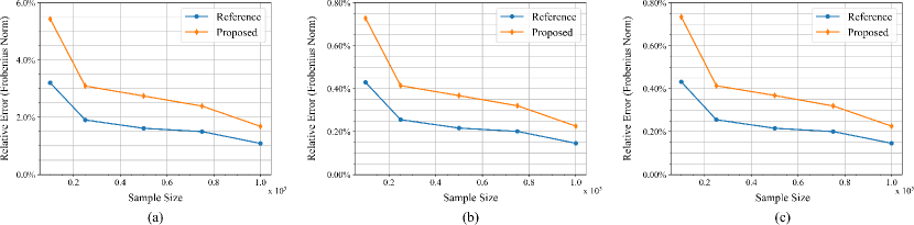
Figure 1: Relative error in estimation of (a) the prior Fisher information $\mathbf{J}_{P}$, (b) the Bayesian information $\mathbf{J}_{B}$, and (c) the Bayesian CRB $\mathbf{V}_{B}$ as a function of sample size. The performance when $\nabla_{\mathbf{x}}\log p(\mathbf{x})$ is known is included as a reference at different sample sizes. As can be seen, the estimation error in the Bayesian information and Bayesian CRB is under $1\%$ in all cases.

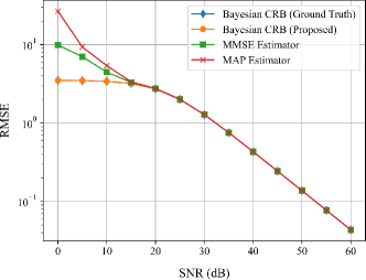
Figure 2: Root-mean-square error (RMSE) as a function of signal-to-noise ratio (SNR) for the ground-truth Bayesian CRB, the proposed estimator, and the minimum mean square error (MMSE) and maximum a posterior (MAP) estimators. Here the proposed estimator was implemented with $N=10^{4}$ samples from the prior distribution, and for each SNR level $20{,}000$ samples from $p(\mathbf{x},\mathbf{y})$ were used to calculate the MAP and MMSE estimators’ RMSEs. The Bayesian CRB estimator is visually identical to the ground truth Bayesian CRB and provides a tight lower bound on the MSE in the high SNR regime.

VII Conclusion

This paper proposed a new data-driven estimator for the Bayesian CRB. The proposed approach incorporates score matching, a statistical estimation technique that underpins a new class of state-of-the-art generative modeling approaches, to model the prior distribution. To characterize the estimator, we considered two different modeling regimes: a classical parametric regime, and a neural network modeling regime, where the score model is a neural network. In both regimes, we proved non-asymptotic bounds on the score matching and Bayesian CRB estimation error. Our proofs draw upon results in empirical process theory, building off of both classical theory and recently developed techniques for characterizing neural networks. We then validated the performance of our estimator on a simple denoising problem with a Gaussian mixture prior, where the estimator was shown to provide accurate estimation performance.

The proposed method assumes that the data model is given, along with a set of i.i.d. samples from the prior distribution. In future work, it would be useful to generalize it to the setting which does not assume explicit knowledge of the data model. It is also of interest to develop regularization techniques for the estimator that provide better sample efficiency in high-dimensional problem settings. Finally, regarding the non-asymptotic estimator bounds, an interesting direction is the development of lower bounds that would provide insight into the optimality of our current results.

Appendix A Proofs for Section IV

This appendix collects various proofs omitted from Section IV in the main text.

Lemma 10.

Suppose $s(\mathbf{x};\boldsymbol{\theta})$ is sufficiently smooth (Assumption IV.2). Then $\ell(\mathbf{x};\boldsymbol{\theta})$ is Lipschitz continuous with Lipschitz constant $L(\mathbf{x})$ and $\mathbb{E}_{\mathbf{x}}\left[L(\mathbf{x})^{2}\right]<\infty$.

Proof.

We have that

$$|\ell(\mathbf{x};\boldsymbol{\theta}_{1})-\ell(\mathbf{x};\boldsymbol{\theta}_{2})| =\left|\text{tr}\left(\nabla_{\mathbf{x}}s(\mathbf{x};\boldsymbol{\theta}_{1})\right)+\frac{1}{2}s(\mathbf{x};\boldsymbol{\theta}_{1})^{T}s(\mathbf{x};\boldsymbol{\theta}_{1})-\left(\text{tr}\left(\nabla_{\mathbf{x}}s(\mathbf{x};\boldsymbol{\theta}_{2})\right)+\frac{1}{2}s(\mathbf{x};\boldsymbol{\theta}_{2})^{T}s(\mathbf{x};\boldsymbol{\theta}_{2})\right)\right|$$

$$\leq\left|\text{tr}\left(\nabla_{\mathbf{x}}s(\mathbf{x};\boldsymbol{\theta}_{1})\right)-\text{tr}\left(\nabla_{\mathbf{x}}s(\mathbf{x};\boldsymbol{\theta}_{2})\right)\right|+\frac{1}{2}\left|s(\mathbf{x};\boldsymbol{\theta}_{1})^{T}s(\mathbf{x};\boldsymbol{\theta}_{1})-s(\mathbf{x};\boldsymbol{\theta}_{2})^{T}s(\mathbf{x};\boldsymbol{\theta}_{2})\right|$$

$$=\sum_{i=1}^{D}\left|\nabla_{\mathbf{x}}s(\mathbf{x};\boldsymbol{\theta}_{1})_{ii}-\nabla_{\mathbf{x}}s(\mathbf{x};\boldsymbol{\theta}_{2})_{ii}\right|+\frac{1}{2}\sum_{i=1}^{D}|s(\mathbf{x};\boldsymbol{\theta}_{1})_{i}^{2}-s(\mathbf{x};\boldsymbol{\theta}_{2})_{i}^{2}|$$

$$\stackrel{{\scriptstyle\footnotesize\mathclap{\mbox{$(i)$}}}}{{\leq}}\sqrt{D}\sqrt{\sum_{i=1}^{D}\left[\nabla_{\mathbf{x}}s(\mathbf{x};\boldsymbol{\theta}_{1})_{ii}-\nabla_{\mathbf{x}}s(\mathbf{x};\boldsymbol{\theta}_{2})_{ii}\right]^{2}}+\frac{\sqrt{D}}{2}\sqrt{\sum_{i=1}^{D}\left[s(\mathbf{x};\boldsymbol{\theta}_{1})_{i}^{2}-s(\mathbf{x};\boldsymbol{\theta}_{2})_{i}^{2}\right]^{2}}$$

$$\leq\sqrt{D}\|\nabla_{\mathbf{x}}s(\mathbf{x};\boldsymbol{\theta}_{1})-\nabla_{\mathbf{x}}s(\mathbf{x};\boldsymbol{\theta}_{2})\|_{2}+\frac{\sqrt{D}}{2}\|s(\mathbf{x};\boldsymbol{\theta}_{1})s(\mathbf{x};\boldsymbol{\theta}_{1})^{T}-s(\mathbf{x};\boldsymbol{\theta}_{2})s(\mathbf{x};\boldsymbol{\theta}_{2})^{T}\|_{2}$$

$$\stackrel{{\scriptstyle\footnotesize\mathclap{\mbox{$(ii)$}}}}{{\leq}}\left[\sqrt{D}L_{1}(\mathbf{x})+\frac{\sqrt{D}}{2}L_{2}(\mathbf{x})\right]\|\boldsymbol{\theta}_{1}-\boldsymbol{\theta}_{2}\|_{2},$$

where $(i)$ is due to the equivalence of finite dimensional norms and $(ii)$ is by Assumption IV.2. So $\ell(\mathbf{x};\boldsymbol{\theta})$ is Lipschitz with a Lipschitz constant bounded by $L(\mathbf{x})\triangleq\sqrt{D}(L_{1}(\mathbf{x})+L_{2}(\mathbf{x})/2)$. Further, we have that

$$\mathbb{E}_{\mathbf{x}}\left[L(\mathbf{x})^{2}\right] =D\mathbb{E}_{\mathbf{x}}\left[L_{1}^{2}(\mathbf{x})+\frac{L_{2}(\mathbf{x})^{2}}{4}+L_{1}(\mathbf{x})L_{2}(\mathbf{x})\right]$$

$$\stackrel{{\scriptstyle\footnotesize\mathclap{\mbox{$(i)$}}}}{{\leq}}D\mathbb{E}_{\mathbf{x}}\left[\frac{3}{2}L_{1}^{2}(\mathbf{x})+\frac{3L_{2}(\mathbf{x})^{2}}{4}\right]\stackrel{{\scriptstyle\footnotesize\mathclap{\mbox{$(ii)$}}}}{{<}}\infty,$$

where $(i)$ is by Young’s inequality and $(ii)$ is due to Assumption IV.2. ∎

Proof of Theorem 1.

By Jensen’s inequality, we have that

$$\mathbb{E}_{\mathbf{x}}\left[\sup_{\boldsymbol{\theta}\in\boldsymbol{\Theta}}\left|\hat{J}(\boldsymbol{\theta};\mathbf{x}_{1}^{N})-J(\boldsymbol{\theta})\right|\right] =\mathbb{E}_{\mathbf{x}}\left[\sup_{\boldsymbol{\theta}\in\boldsymbol{\Theta}}\left|\hat{J}(\boldsymbol{\theta};\mathbf{x}_{1}^{N})-\mathbb{E}_{\mathbf{x}}\left[\hat{J}(\boldsymbol{\theta};\mathbf{x}_{1}^{N})\right]\right|\right]$$

$$=\mathbb{E}_{\mathbf{x}}\left[\sup_{\boldsymbol{\theta}\in\boldsymbol{\Theta}}\left|\hat{J}(\boldsymbol{\theta};\mathbf{x}_{1}^{N})-\mathbb{E}_{\mathbf{x}^{\prime}}\left[\hat{J}(\boldsymbol{\theta};{\mathbf{x}^{\prime}}_{1}^{N})\right]\right|\right]$$

$$\leq\mathbb{E}_{\mathbf{x},\mathbf{x}^{\prime}}\left[\sup_{\boldsymbol{\theta}\in\boldsymbol{\Theta}}\left|\hat{J}(\boldsymbol{\theta};\mathbf{x}_{1}^{N})-\hat{J}(\boldsymbol{\theta};{\mathbf{x}^{\prime}}_{1}^{N})\right|\right],$$

where ${\mathbf{x}^{\prime}}_{1}^{N}$ is an independent copy of $\mathbf{x}_{1}^{N}$. Now let $\{\epsilon_{i}\}_{i=1}^{N}$ be a set of independent Rademacher (symmetric Bernoulli) random variables. Since $\ell(\mathbf{x}_{i};\boldsymbol{\theta})-\ell({\mathbf{x}^{\prime}}_{i};\boldsymbol{\theta})$ is symmetric around zero, we have that

$${\mathbb{E}_{\mathbf{x},\mathbf{x}^{\prime}}}\left[\sup_{\boldsymbol{\theta}\in\boldsymbol{\Theta}}\left|\hat{J}(\boldsymbol{\theta};\mathbf{x}_{1}^{N})-\hat{J}(\boldsymbol{\theta};{\mathbf{x}^{\prime}}_{1}^{N})\right|\right] =\mathbb{E}_{\mathbf{x},\mathbf{x}^{\prime}}\left[\sup_{\boldsymbol{\theta}\in\boldsymbol{\Theta}}\left|\frac{1}{N}\sum_{i=1}^{N}\ell(\mathbf{x}_{i};\boldsymbol{\theta})-\ell({\mathbf{x}^{\prime}}_{i};\boldsymbol{\theta})\right|\right]$$

$$=\mathbb{E}_{\mathbf{x},\mathbf{x}^{\prime},\epsilon}\left[\sup_{\boldsymbol{\theta}\in\boldsymbol{\Theta}}\left|\frac{1}{N}\sum_{i=1}^{N}\epsilon_{i}\left[\ell(\mathbf{x}_{i};\boldsymbol{\theta})-\ell({\mathbf{x}^{\prime}}_{i};\boldsymbol{\theta})\right]\right|\right].$$

We then fix a $\boldsymbol{\theta}^{\prime}\in\boldsymbol{\Theta}$ to obtain

$$\mathbb{E}_{\mathbf{x},\mathbf{x}^{\prime},\epsilon} \left[\sup_{\boldsymbol{\theta}\in\boldsymbol{\Theta}}\left|\frac{1}{N}\sum_{i=1}^{N}\epsilon_{i}\left[\ell(\mathbf{x}_{i};\boldsymbol{\theta})-\ell({\mathbf{x}^{\prime}}_{i};\boldsymbol{\theta})\right]\right|\right]$$

$$=\mathbb{E}_{\mathbf{x},\mathbf{x}^{\prime},\epsilon}\left[\sup_{\boldsymbol{\theta}\in\boldsymbol{\Theta}}\left|\frac{1}{N}\sum_{i=1}^{N}\epsilon_{i}\left[\ell(\mathbf{x}_{i};\boldsymbol{\theta})-\ell(\mathbf{x}_{i};\boldsymbol{\theta}^{\prime})+\ell(\mathbf{x}_{i};\boldsymbol{\theta}^{\prime})-\ell({\mathbf{x}^{\prime}}_{i};\boldsymbol{\theta})\right]\right|\right]$$

$$\leq\mathbb{E}_{\mathbf{x},\epsilon}\left[\sup_{\boldsymbol{\theta}\in\boldsymbol{\Theta}}\left|\frac{1}{N}\sum_{i=1}^{N}\epsilon_{i}\left[\ell(\mathbf{x}_{i};\boldsymbol{\theta})-\ell(\mathbf{x}_{i};\boldsymbol{\theta}^{\prime})\right]\right|\right]+\mathbb{E}_{\mathbf{x},\mathbf{x}^{\prime}\epsilon}\left[\sup_{\boldsymbol{\theta}\in\boldsymbol{\Theta}}\left|\frac{1}{N}\sum_{i=1}^{N}\epsilon_{i}\left[\ell(\mathbf{x}_{i};\boldsymbol{\theta}^{\prime})-\ell({\mathbf{x}^{\prime}}_{i};\boldsymbol{\theta})\right]\right|\right]$$

$$=\mathbb{E}_{\mathbf{x},\epsilon}\left[\sup_{\boldsymbol{\theta}\in\boldsymbol{\Theta}}\left|\frac{1}{N}\sum_{i=1}^{N}\epsilon_{i}\left[\ell(\mathbf{x}_{i};\boldsymbol{\theta})-\ell(\mathbf{x}_{i};\boldsymbol{\theta}^{\prime})\right]\right|\right]$$

$$\quad\quad+\mathbb{E}_{\mathbf{x},\mathbf{x}^{\prime}\epsilon}\left[\sup_{\boldsymbol{\theta}\in\boldsymbol{\Theta}}\left|\frac{1}{N}\sum_{i=1}^{N}\epsilon_{i}\left[\ell(\mathbf{x}_{i};\boldsymbol{\theta}^{\prime})-\ell({\mathbf{x}^{\prime}}_{i};\boldsymbol{\theta}^{\prime})+\ell({\mathbf{x}^{\prime}}_{i};\boldsymbol{\theta}^{\prime})-\ell({\mathbf{x}^{\prime}}_{i};\boldsymbol{\theta})\right]\right|\right]$$

$$\leq\mathbb{E}_{\mathbf{x},\epsilon}\left[\sup_{\boldsymbol{\theta}\in\boldsymbol{\Theta}}\left|\frac{1}{N}\sum_{i=1}^{N}\epsilon_{i}\left[\ell(\mathbf{x}_{i};\boldsymbol{\theta})-\ell(\mathbf{x}_{i};\boldsymbol{\theta}^{\prime})\right]\right|\right]+\mathbb{E}_{\mathbf{x},\mathbf{x}^{\prime},\epsilon}\left[\left|\frac{1}{N}\sum_{i=1}^{N}\epsilon_{i}\left[\ell(\mathbf{x}_{i};\boldsymbol{\theta}^{\prime})-\ell({\mathbf{x}^{\prime}}_{i};\boldsymbol{\theta}^{\prime})\right]\right|\right]$$

$$\quad\quad+\mathbb{E}_{\mathbf{x}^{\prime},\epsilon}\left[\sup_{\boldsymbol{\theta}\in\boldsymbol{\Theta}}\left|\frac{1}{N}\sum_{i=1}^{N}\epsilon_{i}\left[\ell(\mathbf{x}^{\prime}_{i};\boldsymbol{\theta}^{\prime})-\ell(\mathbf{x}^{\prime}_{i};\boldsymbol{\theta})\right]\right|\right]$$

$$=2\mathbb{E}_{\mathbf{x},\epsilon}\left[\sup_{\boldsymbol{\theta}\in\boldsymbol{\Theta}}\left|\frac{1}{N}\sum_{i=1}^{N}\epsilon_{i}\left[\ell(\mathbf{x}_{i};\boldsymbol{\theta})-\ell(\mathbf{x}_{i};\boldsymbol{\theta}^{\prime})\right]\right|\right]+\mathbb{E}_{\mathbf{x},\mathbf{x}^{\prime},\epsilon}\left[\left|\frac{1}{N}\sum_{i=1}^{N}\epsilon_{i}\left[\ell(\mathbf{x}^{\prime}_{i};\boldsymbol{\theta}^{\prime})-\ell(\mathbf{x}_{i};\boldsymbol{\theta}^{\prime})\right]\right|\right]$$ (30)

through repeated application of the triangle inequality.

The above expression has two terms. The second term does not involve a supremum and can be straightforwardly bounded by the law of large numbers. Specifically, we have that

$$\mathbb{E}_{\mathbf{x},\mathbf{x}^{\prime},\epsilon}\left[\left|\frac{1}{N}\sum_{i=1}^{N}\epsilon_{i}\left[\ell({\mathbf{x}^{\prime}}_{i};\boldsymbol{\theta}^{\prime})-\ell(\mathbf{x}_{i};\boldsymbol{\theta}^{\prime})\right]\right|\right] =\mathbb{E}_{\mathbf{x},\mathbf{x}^{\prime}}\left[\left|\frac{1}{N}\sum_{i=1}^{N}\left[\ell({\mathbf{x}^{\prime}}_{i};\boldsymbol{\theta}^{\prime})-\ell(\mathbf{x}_{i};\boldsymbol{\theta}^{\prime})\right]\right|\right]$$

$$=\mathbb{E}_{\mathbf{x},\mathbf{x}^{\prime}}\left[\left|\frac{1}{N}\sum_{i=1}^{N}\left[\ell({\mathbf{x}^{\prime}}_{i};\boldsymbol{\theta}^{\prime})-J(\boldsymbol{\theta}^{\prime})+J(\boldsymbol{\theta}^{\prime})-\ell(\mathbf{x}_{i};\boldsymbol{\theta}^{\prime})\right]\right|\right]$$

$$\leq\mathbb{E}_{\mathbf{x}}\left[\left|\hat{J}(\boldsymbol{\theta}^{\prime},\mathbf{x}_{1}^{N})-J(\boldsymbol{\theta}^{\prime})\right|\right]+\mathbb{E}_{\mathbf{x}^{\prime}}\left[\left|\hat{J}(\boldsymbol{\theta}^{\prime},{\mathbf{x}^{\prime}}_{1}^{N})-J(\boldsymbol{\theta}^{\prime})\right|\right]$$

$$=2\mathbb{E}_{\mathbf{x}}\left[\left|\hat{J}(\boldsymbol{\theta}^{\prime},\mathbf{x}_{1}^{N})-J(\boldsymbol{\theta}^{\prime})\right|\right]=O\left(\frac{1}{\sqrt{N}}\right).$$ (31)

To bound the first term, note that for any fixed $\mathbf{x}_{1}^{N}$, the random variable $\frac{1}{N}\sum_{i=1}^{N}\epsilon_{i}\ell(\mathbf{x}_{i};\boldsymbol{\theta})$ is a sub-Gaussian process (see, e.g., Definition 5.16 in [33]) with respect to $\boldsymbol{\theta}$, i.e., for any $\boldsymbol{\theta}_{1},\boldsymbol{\theta}_{2}\in\boldsymbol{\Theta}$, $\mathbf{x}_{1}^{N}$, and $\lambda\in\mathbb{R}$, we have that

$$\mathbb{E}_{\epsilon}\left[e^{\lambda\frac{1}{N}\sum_{i=1}^{N}\epsilon_{i}\left[\ell(\mathbf{x}_{i};\boldsymbol{\theta}_{1})-\ell(\mathbf{x}_{i};\boldsymbol{\theta}_{2})\right]}\right] \stackrel{{\scriptstyle\footnotesize\mathclap{\mbox{$(i)$}}}}{{=}}\prod_{i=1}^{N}\mathbb{E}_{\epsilon}\left[e^{\lambda\frac{1}{N}\epsilon_{i}\left[\ell(\mathbf{x}_{i};\boldsymbol{\theta}_{1})-\ell(\mathbf{x}_{i};\boldsymbol{\theta}_{2})\right]}\right]$$

$$\stackrel{{\scriptstyle\footnotesize\mathclap{\mbox{$(ii)$}}}}{{\leq}}\prod_{i=1}^{N}\mathrm{exp}\left(\frac{\lambda^{2}}{2N^{2}}\left[\ell(\mathbf{x}_{i};\boldsymbol{\theta}_{1})-\ell(\mathbf{x}_{i};\boldsymbol{\theta}_{2})\right]^{2}\right)$$

$$\stackrel{{\scriptstyle\footnotesize\mathclap{\mbox{$(iii)$}}}}{{\leq}}\prod_{i=1}^{N}\mathrm{exp}\left(\frac{\lambda^{2}}{2N^{2}}L^{2}(\mathbf{x}_{i})\|\boldsymbol{\theta}_{1}-\boldsymbol{\theta}_{2}\|_{2}^{2}\right)$$

$$=\mathrm{exp}\left(\sum_{i=1}^{N}\frac{\lambda^{2}}{2N^{2}}L^{2}(\mathbf{x}_{i})\|\boldsymbol{\theta}_{1}-\boldsymbol{\theta}_{2}\|_{2}^{2}\right).$$

Here $(i)$ is by independence of the $\epsilon_{i}$, $(ii)$ is because $\mathbb{E}_{\epsilon}\left[e^{\beta\epsilon}\right]\leq e^{\beta^{2}/2}$ for all $\beta\in\mathbb{R}$, and $(iii)$ is by Lemma 10. This shows that $\frac{1}{N}\sum_{i=1}^{N}\epsilon_{i}\ell(\mathbf{x}_{i};\boldsymbol{\theta})$ is a sub-Gaussian process with metric

$$d(\boldsymbol{\theta}_{1},\boldsymbol{\theta}_{2})\triangleq\frac{1}{\sqrt{N}}\sqrt{\frac{1}{N}\sum_{i=1}^{N}L^{2}(\mathbf{x}_{i})}\|\boldsymbol{\theta}_{1}-\boldsymbol{\theta}_{2}\|_{2}.$$

Now, since $\boldsymbol{\Theta}$ is compact, the diameter of $\boldsymbol{\Theta}$ with respect to the Euclidean norm is finite, and we denote it as $\mathrm{diam}(\boldsymbol{\Theta})$. Using Dudley’s entropy integral [34], we can conclude that

$$\mathbb{E}_{\mathbf{x},\epsilon}\left[\sup_{\boldsymbol{\theta}\in\boldsymbol{\Theta}}\left|\frac{1}{N}\sum_{i=1}^{N}\epsilon_{i}\left[\ell(\mathbf{x}_{i};\boldsymbol{\theta})-\ell(\mathbf{x}_{i};\boldsymbol{\theta}^{\prime})\right]\right|\right]\leq O(1)\mathbb{E}_{\mathbf{x}}\left[\int_{0}^{\frac{1}{\sqrt{N}}\sqrt{\frac{1}{N}\sum_{i=1}^{N}L^{2}(\mathbf{x}_{i})}\mathrm{diam}(\boldsymbol{\Theta})}\sqrt{\log N(\boldsymbol{\Theta},d,\epsilon)}\;d\epsilon\right].$$ (32)

Here $\log N(\boldsymbol{\Theta},d,\epsilon)$ is the metric entropy, i.e., the log of the $\epsilon$-covering number, of $\boldsymbol{\Theta}$ with respect to the metric $d(\boldsymbol{\theta}_{1},\boldsymbol{\theta}_{2})=\frac{1}{\sqrt{N}}\sqrt{\frac{1}{N}\sum_{i=1}^{N}L^{2}(\mathbf{x}_{i})}\|\boldsymbol{\theta}_{1}-\boldsymbol{\theta}_{2}\|_{2}$.

It is known that the $\epsilon$-covering number of $\boldsymbol{\Theta}$ with the canonical Euclidean metric satisfies

$$N(\boldsymbol{\Theta},\|\cdot\|_{2},\epsilon)\leq\left(1+\frac{\mathrm{diam}(\boldsymbol{\Theta})}{\epsilon}\right)^{P}.$$

We can therefore bound $N(\boldsymbol{\Theta},d,\epsilon)$ by

$$N(\boldsymbol{\Theta},d,\epsilon)\leq\left(1+\sqrt{\frac{1}{N}\sum_{i=1}^{N}L^{2}(\mathbf{x}_{i})}\frac{\mathrm{diam}(\boldsymbol{\Theta})}{\sqrt{N}\epsilon}\right)^{P}.$$

Using this bound, we can bound the metric entropy integral as follows:

$$\int_{0}^{\frac{1}{\sqrt{N}}\sqrt{\frac{1}{N}\sum_{i=1}^{N}L^{2}(\mathbf{x}_{i})}\mathrm{diam}(\boldsymbol{\Theta})}\sqrt{\log N(\boldsymbol{\Theta},d,\epsilon)}\;d\epsilon$$

$$\quad\quad\quad\leq\int_{0}^{\frac{1}{\sqrt{N}}\sqrt{\frac{1}{N}\sum_{i=1}^{N}L^{2}(\mathbf{x}_{i})}\mathrm{diam}(\boldsymbol{\Theta})}\sqrt{P\log\left(1+\sqrt{\frac{1}{N}\sum_{i=1}^{N}L^{2}(\mathbf{x}_{i})}\frac{\mathrm{diam}(\boldsymbol{\Theta})}{\sqrt{N}\epsilon}\right)}d\epsilon$$

$$\quad\quad\quad\stackrel{{\scriptstyle\footnotesize\mathclap{\mbox{$(i)$}}}}{{\leq}}\int_{0}^{\frac{1}{\sqrt{N}}\sqrt{\frac{1}{N}\sum_{i=1}^{N}L^{2}(\mathbf{x}_{i})}\mathrm{diam}(\boldsymbol{\Theta})}\sqrt{\sqrt{\frac{1}{N}\sum_{i=1}^{N}L^{2}(\mathbf{x}_{i})}\frac{P\mathrm{diam}(\boldsymbol{\Theta})}{\sqrt{N}\epsilon}}\;d\epsilon$$

$$\quad\quad\quad=2\sqrt{\frac{1}{N}\sum_{i=1}^{N}L^{2}(\mathbf{x}_{i})}\sqrt{\frac{P}{N}}\mathrm{diam}(\boldsymbol{\Theta}),$$ (33)

where here $(i)$ holds because $\log(1+x)\leq x$ for all $x\geq 0$. Finally, combining (A), (A), (32) and (A) gives

$$\mathbb{E}_{\mathbf{x}}\left[\sup_{\boldsymbol{\theta}\in\boldsymbol{\Theta}}\left|\hat{J}(\boldsymbol{\theta};\mathbf{x}_{1}^{N})-J(\boldsymbol{\theta})\right|\right] \leq 4O(1)\mathbb{E}_{\mathbf{x}}\left[\sqrt{\frac{1}{N}\sum_{i=1}^{N}L^{2}(\mathbf{x}_{i})}\sqrt{\frac{P}{N}}\mathrm{diam}(\boldsymbol{\Theta})\right]+O\left(\frac{1}{\sqrt{N}}\right)$$

$$\stackrel{{\scriptstyle\footnotesize\mathclap{\mbox{$(i)$}}}}{{\leq}}O(1)\sqrt{\frac{P}{N}}\mathrm{diam}(\boldsymbol{\Theta})\sqrt{\mathbb{E}_{\mathbf{x}}\left[\frac{1}{N}\sum_{i=1}^{N}L^{2}(\mathbf{x}_{i})\right]}+O\left(\frac{1}{\sqrt{N}}\right)$$

$$\stackrel{{\scriptstyle\footnotesize\mathclap{\mbox{$(ii)$}}}}{{=}}O\left(\frac{1+\mathrm{diam}\left(\boldsymbol{\Theta}\right)\sqrt{P}}{\sqrt{N}}\right),$$

where $(i)$ is due to Jensen’s inequality and $(ii)$ holds because Lemma 10 guarantees that the expectation is finite. Setting $C_{S}\triangleq O(1+\mathrm{diam}\left(\boldsymbol{\Theta}\right)\sqrt{P})$ completes the proof. ∎

Proof of Corollary 1.

By Jensen’s inequality, we have that

$$\mathbb{E}_{\mathbf{x}}\left[\sup_{\|\boldsymbol{\theta}-\boldsymbol{\theta}^{*}\|_{2}\leq\delta}\left|\Delta_{N}(\boldsymbol{\theta})\right|\right] =\mathbb{E}_{\mathbf{x}}\left[\sup_{\|\boldsymbol{\theta}-\boldsymbol{\theta}^{*}\|_{2}\leq\delta}\left|(\hat{J}(\boldsymbol{\theta};\mathbf{x}_{1}^{N})-J(\boldsymbol{\theta}))-(\hat{J}(\boldsymbol{\theta}^{*};\mathbf{x}_{1}^{N})-J(\boldsymbol{\theta}^{*}))\right|\right]$$

$$=\mathbb{E}_{\mathbf{x}}\left[\sup_{\|\boldsymbol{\theta}-\boldsymbol{\theta}^{*}\|_{2}\leq\delta}\left|(\hat{J}(\boldsymbol{\theta};\mathbf{x}_{1}^{N})-\hat{J}(\boldsymbol{\theta}^{*};\mathbf{x}_{1}^{N}))-\mathbb{E}_{\mathbf{x}^{\prime}}\left[\hat{J}(\boldsymbol{\theta};{\mathbf{x}^{\prime}}_{1}^{N})-\hat{J}(\boldsymbol{\theta}^{*};{\mathbf{x}^{\prime}}_{1}^{N})\right]\right|\right]$$

$$\leq\mathbb{E}_{\mathbf{x},\mathbf{x}^{\prime}}\left[\sup_{\|\boldsymbol{\theta}-\boldsymbol{\theta}^{*}\|_{2}\leq\delta}\left|(\hat{J}(\boldsymbol{\theta};\mathbf{x}_{1}^{N})-\hat{J}(\boldsymbol{\theta};{\mathbf{x}^{\prime}}_{1}^{N}))-(\hat{J}(\boldsymbol{\theta}^{*};\mathbf{x}_{1}^{N})-\hat{J}(\boldsymbol{\theta}^{*};{\mathbf{x}^{\prime}}_{1}^{N}))\right|\right].$$

Now let $\{\epsilon_{i}\}_{i=1}^{N}$ be a set of independent Rademacher random variables. We have that

$$\mathbb{E}_{\mathbf{x},\mathbf{x}^{\prime}} \left[\sup_{\|\boldsymbol{\theta}-\boldsymbol{\theta}^{*}\|_{2}\leq\delta}\left|(\hat{J}(\boldsymbol{\theta};\mathbf{x}_{1}^{N})-\hat{J}(\boldsymbol{\theta};{\mathbf{x}^{\prime}}_{1}^{N}))-(\hat{J}(\boldsymbol{\theta}^{*};\mathbf{x}_{1}^{N})-\hat{J}(\boldsymbol{\theta}^{*};{\mathbf{x}^{\prime}}_{1}^{N}))\right|\right]$$

$$\hskip 56.9055pt=\mathbb{E}_{\mathbf{x},\mathbf{x}^{\prime}}\left[\sup_{\|\boldsymbol{\theta}-\boldsymbol{\theta}^{*}\|_{2}\leq\delta}\left|\frac{1}{N}\sum_{i=1}^{N}(\ell(\mathbf{x}_{i};\boldsymbol{\theta})-\ell({\mathbf{x}^{\prime}}_{i};\boldsymbol{\theta}))-(\ell(\mathbf{x}_{i};\boldsymbol{\theta}^{*})-\ell({\mathbf{x}^{\prime}}_{i};\boldsymbol{\theta}^{*}))\right|\right]$$

$$\hskip 56.9055pt\stackrel{{\scriptstyle\footnotesize\mathclap{\mbox{$(i)$}}}}{{=}}\mathbb{E}_{\mathbf{x},\mathbf{x}^{\prime},\epsilon}\left[\sup_{\|\boldsymbol{\theta}-\boldsymbol{\theta}^{*}\|_{2}\leq\delta}\left|\frac{1}{N}\sum_{i=1}^{N}\epsilon_{i}(\ell(\mathbf{x}_{i};\boldsymbol{\theta})-\ell({\mathbf{x}^{\prime}}_{i};\boldsymbol{\theta}))-\epsilon_{i}(\ell(\mathbf{x}_{i};\boldsymbol{\theta}^{*})-\ell({\mathbf{x}^{\prime}}_{i};\boldsymbol{\theta}^{*}))\right|\right]$$

$$\hskip 56.9055pt\leq\mathbb{E}_{\mathbf{x},\epsilon}\left[\sup_{\|\boldsymbol{\theta}-\boldsymbol{\theta}^{*}\|_{2}\leq\delta}\left|\frac{1}{N}\sum_{i=1}^{N}\epsilon_{i}(\ell(\mathbf{x}_{i};\boldsymbol{\theta})-\ell(\mathbf{x}_{i};\boldsymbol{\theta}^{*}))\right|\right]$$

$$\hskip 85.35826pt+\mathbb{E}_{\mathbf{x}^{\prime},\epsilon}\left[\sup_{\|\boldsymbol{\theta}-\boldsymbol{\theta}^{*}\|_{2}\leq\delta}\left|\frac{1}{N}\sum_{i=1}^{N}\epsilon_{i}(\ell({\mathbf{x}^{\prime}}_{i};\boldsymbol{\theta})-\ell({\mathbf{x}^{\prime}}_{i};\boldsymbol{\theta}^{*}))\right|\right]$$

$$\hskip 56.9055pt=2\mathbb{E}_{\mathbf{x},\epsilon}\left[\sup_{\|\boldsymbol{\theta}-\boldsymbol{\theta}^{*}\|_{2}\leq\delta}\left|\frac{1}{N}\sum_{i=1}^{N}\epsilon_{i}(\ell(\mathbf{x}_{i};\boldsymbol{\theta})-\ell(\mathbf{x}_{i};\boldsymbol{\theta}^{*}))\right|\right],$$

where $(i)$ holds because $\ell(\mathbf{x}_{i};\boldsymbol{\theta})-\ell({\mathbf{x}^{\prime}}_{i};\boldsymbol{\theta})$ is symmetric around zero.

The rest of the proof is similar to that of Theorem 9 and is therefore omitted.

∎

Proof of Theorem 2.

The proof is based on a partition of the parameter space into the following collection of “shells”:

$$S_{N,j}\triangleq\{\boldsymbol{\theta}\in\boldsymbol{\Theta}\,:\,2^{j}<\sqrt{N}\|\boldsymbol{\theta}-\boldsymbol{\theta}^{*}\|_{2}\leq 2^{j+1}\}.$$

Specifically, letting $T\triangleq 8C_{\boldsymbol{\theta}}\sqrt{P}/\epsilon\lambda$, we have that

$$\mathbb{P}\left[\sqrt{N}\|\hat{\boldsymbol{\theta}}_{N}-\boldsymbol{\theta}^{*}\|_{2}>T\right] \leq\mathbb{P}\left[\sqrt{N}\|\hat{\boldsymbol{\theta}}_{N}-\boldsymbol{\theta}^{*}\|_{2}>T,\|\hat{\boldsymbol{\theta}}_{N}-\boldsymbol{\theta}^{*}\|_{2}\leq\eta\right]+\mathbb{P}\left[\|\hat{\boldsymbol{\theta}}_{N}-\boldsymbol{\theta}^{*}\|_{2}>\eta\right]$$

$$\leq\mathbb{P}[\exists j\geq\log_{2}\left(T\right)\text{ such that }2^{j}\leq\sqrt{N}\eta\text{ and }\hat{\boldsymbol{\theta}}_{N}\in S_{N,j}]+\mathbb{P}\left[\|\hat{\boldsymbol{\theta}}_{N}-\boldsymbol{\theta}^{*}\|_{2}>\eta\right]$$

$$\leq\sum_{j\geq\log_{2}\left(T\right),2^{j}\leq\sqrt{N}\eta}\mathbb{P}[\hat{\boldsymbol{\theta}}_{N}\in S_{N,j}]+\mathbb{P}\left[\|\hat{\boldsymbol{\theta}}_{N}-\boldsymbol{\theta}^{*}\|_{2}>\eta\right]$$ (34)

where $\eta$ is defined by Assumption IV.4. By Lemma 1, we have that for all $N\geq 16C_{S}^{2}/\epsilon^{2}\lambda^{2}\eta^{4}$, it holds that

$$\mathbb{P}\left[\|\hat{\boldsymbol{\theta}}_{N}-\boldsymbol{\theta}^{*}\|_{2}>\eta\right]\leq\frac{\epsilon}{2},$$ (35)

which bounds the second term in (A).

To bound the first term, assume $\hat{\boldsymbol{\theta}}_{N}\in S_{N,j}$. Then there exists $\boldsymbol{\theta}\in S_{N,j}$ such that $\hat{J}(\boldsymbol{\theta};\mathbf{x}_{1}^{N})\leq\hat{J}(\boldsymbol{\theta}^{*};\mathbf{x}_{1}^{N})$. By Assumption IV.4, we have that

$$\Delta_{N}(\boldsymbol{\theta}) =(\hat{J}(\boldsymbol{\theta};\mathbf{x}_{1}^{N})-\hat{J}(\boldsymbol{\theta}^{*};\mathbf{x}_{1}^{N}))+(J(\boldsymbol{\theta}^{*})-J(\boldsymbol{\theta}))$$

$$\leq J(\boldsymbol{\theta}^{*})-J(\boldsymbol{\theta})\leq-\lambda\|\boldsymbol{\theta}-\boldsymbol{\theta}^{*}\|_{2}^{2},$$

which implies that

$$|\Delta_{N}(\boldsymbol{\theta})|\geq\lambda\|\boldsymbol{\theta}-\boldsymbol{\theta}^{*}\|_{2}^{2}>\lambda\frac{4^{j}}{N}.$$

This allows us to rewrite $\mathbb{P}[\hat{\boldsymbol{\theta}}_{N}\in S_{N,j}]$ in terms of $\Delta_{N}(\boldsymbol{\theta})$; we have that

$$\mathbb{P}[\hat{\boldsymbol{\theta}}_{N}\in S_{N,j}] \leq\mathbb{P}\left(\exists\boldsymbol{\theta}\in S_{N,j}\text{ such that }|\Delta_{N}(\boldsymbol{\theta})|>\lambda\frac{4^{j}}{N}\right)$$

$$\leq\mathbb{P}\left(\text{sup}_{\boldsymbol{\theta}\in S_{N,j}}|\Delta_{N}(\boldsymbol{\theta})|>\lambda\frac{4^{j}}{N}\right)$$

$$\stackrel{{\scriptstyle\footnotesize\mathclap{\mbox{$(i)$}}}}{{\leq}}\frac{\mathbb{E}_{\mathbf{x}}\left[\text{sup}_{\boldsymbol{\theta}\in S_{N,j}}|\Delta_{N}(\boldsymbol{\theta})|\right]}{\frac{\lambda 4^{j}}{N}},$$

where $(i)$ is due to Markov’s inequality. Since $\boldsymbol{\theta}\in S_{N,j}$ implies $\|\boldsymbol{\theta}-\boldsymbol{\theta}^{*}\|_{2}\leq 2^{j+1}/\sqrt{N}$, by Corollary 1 this supremum can be bounded, i.e., we have that

$$\mathbb{P}[\hat{\boldsymbol{\theta}}_{N}\in S_{N,j}]\leq\frac{\mathbb{E}_{\mathbf{x}}\left[\text{sup}_{\boldsymbol{\theta}\in S_{N,j}}|\Delta_{N}(\boldsymbol{\theta})|\right]}{\lambda\frac{4^{j}}{N}}\leq\frac{N}{\lambda 4^{j}}C_{\boldsymbol{\theta}}\sqrt{P}\frac{2^{j+1}}{\sqrt{N}}\frac{1}{\sqrt{N}}\leq\frac{C_{\boldsymbol{\theta}}\sqrt{P}}{\lambda 2^{j-1}}.$$

Now note that for any $\epsilon>0$, we have that

$$\sum_{j\geq\log_{2}\left(T\right),2^{j}\leq\sqrt{N}\eta}\mathbb{P}[\hat{\boldsymbol{\theta}}_{N}\in S_{N,j}]\leq\sum_{j\geq\log_{2}\left(T\right)}\frac{C_{\boldsymbol{\theta}}\sqrt{P}}{\lambda 2^{j-1}}=\frac{2C_{\boldsymbol{\theta}}\sqrt{P}}{\lambda}\sum_{j\geq\log_{2}\left(T\right)}\frac{1}{2^{j}}=\frac{2C_{\boldsymbol{\theta}}\sqrt{P}}{\lambda}\frac{2}{T}=\frac{\epsilon}{2}.$$ (36)

Plugging in (35) and (36) into (A) gives

$$\mathbb{P}\left[\sqrt{N}\|\hat{\boldsymbol{\theta}}_{N}-\boldsymbol{\theta}^{*}\|_{2}>T\right]\leq\sum_{j\geq\log_{2}\left(T\right),2^{j}\leq\sqrt{N}\eta}\mathbb{P}[\hat{\boldsymbol{\theta}}_{N}\in S_{N,j}]+\mathbb{P}\left[\|\hat{\boldsymbol{\theta}}_{N}-\boldsymbol{\theta}^{*}\|_{2}>\eta\right]\leq\frac{\epsilon}{2}+\frac{\epsilon}{2}=\epsilon$$

for all $N\geq N^{\prime}$, as desired.

∎

Proof of Theorem 3.

First, note that the $\mathbf{J}_{B}$ estimation error can be bounded as follows:

$$\|\hat{\mathbf{J}}_{B}(\mathbf{x}_{1}^{N})-\mathbf{J}_{B}\|_{\sigma} =\left\lVert\frac{1}{N}\sum_{i=1}^{N}s(\mathbf{x}_{i};\hat{\boldsymbol{\theta}}_{N})s(\mathbf{x}_{i};\hat{\boldsymbol{\theta}}_{N})^{T}+\hat{\mathbf{J}}_{F}(\mathbf{x}_{i})-(\mathbf{J}_{P}+\mathbf{J}_{D})\right\rVert_{\sigma}$$

$$\leq\left\lVert\frac{1}{N}\sum_{i=1}^{N}s(\mathbf{x}_{i};\hat{\boldsymbol{\theta}}_{N})s(\mathbf{x}_{i};\hat{\boldsymbol{\theta}}_{N})^{T}-\mathbf{J}_{P}\right\rVert_{\sigma}+\left\lVert\frac{1}{N}\sum_{i=1}^{N}\hat{\mathbf{J}}_{F}(\mathbf{x}_{i})-\mathbf{J}_{D}\right\rVert_{\sigma}$$

$$\leq\left\lVert\frac{1}{N}\sum_{i=1}^{N}s(\mathbf{x}_{i};\hat{\boldsymbol{\theta}}_{N})s(\mathbf{x}_{i};\hat{\boldsymbol{\theta}}_{N})^{T}-\frac{1}{N}\sum_{i=1}^{N}s(\mathbf{x}_{i};\boldsymbol{\theta}^{*})s(\mathbf{x}_{i};\boldsymbol{\theta}^{*})^{T}\right\rVert_{\sigma}$$

$$\quad+\left\lVert\frac{1}{N}\sum_{i=1}^{N}s(\mathbf{x}_{i};\boldsymbol{\theta}^{*})s(\mathbf{x}_{i};\boldsymbol{\theta}^{*})^{T}-\frac{1}{N}\sum_{i=1}^{N}\nabla_{\mathbf{x}}\log p(\mathbf{x}_{i})\nabla_{\mathbf{x}}\log p(\mathbf{x}_{i})^{T}\right\rVert_{\sigma}$$

$$\quad+\left\lVert\frac{1}{N}\sum_{i=1}^{N}\nabla_{\mathbf{x}}\log p(\mathbf{x}_{i})\nabla_{\mathbf{x}}\log p(\mathbf{x}_{i})^{T}-\mathbf{J}_{P}\right\rVert_{\sigma}+\left\lVert\frac{1}{N}\sum_{i=1}^{N}\hat{\mathbf{J}}_{F}(\mathbf{x}_{i})-\mathbf{J}_{D}\right\rVert_{\sigma}.$$

We now bound the four terms in the above expression. For the first term, by Theorem 2 we have that

$$\|\hat{\boldsymbol{\theta}}_{N}-\boldsymbol{\theta}^{*}\|_{2}\leq\frac{8C_{\boldsymbol{\theta}}\sqrt{P}}{\epsilon\lambda\sqrt{N}}$$

with probability at least $1-\epsilon$ for all $N\geq N^{\prime}$. Using this fact and Assumption IV.2, it holds that

$$\left\lVert\frac{1}{N}\sum_{i=1}^{N}\left(s(\mathbf{x}_{i};\hat{\boldsymbol{\theta}}_{N})s(\mathbf{x}_{i};\hat{\boldsymbol{\theta}}_{N})^{T}-s(\mathbf{x}_{i};\boldsymbol{\theta}^{*})s(\mathbf{x}_{i};\boldsymbol{\theta}^{*})^{T}\right)\right\rVert_{\sigma} \leq\left\lVert\frac{1}{N}\sum_{i=1}^{N}\left(s(\mathbf{x}_{i};\hat{\boldsymbol{\theta}}_{N})s(\mathbf{x}_{i};\hat{\boldsymbol{\theta}}_{N})^{T}-s(\mathbf{x}_{i};\boldsymbol{\theta}^{*})s(\mathbf{x}_{i};\boldsymbol{\theta}^{*})^{T}\right)\right\rVert_{2}$$

$$\leq\frac{1}{N}\sum_{i=1}^{N}\left\lVert s(\mathbf{x}_{i};\hat{\boldsymbol{\theta}}_{N})s(\mathbf{x}_{i};\hat{\boldsymbol{\theta}}_{N})^{T}-s(\mathbf{x}_{i};\boldsymbol{\theta}^{*})s(\mathbf{x}_{i};\boldsymbol{\theta}^{*})^{T}\right\rVert_{2}$$

$$\leq\left[\frac{1}{N}\sum_{i=1}^{N}L_{2}(\mathbf{x}_{i})\right]\frac{8C_{\boldsymbol{\theta}}\sqrt{P}}{\epsilon\lambda\sqrt{N}}$$ (37)

for all $N\geq N^{\prime}$ with probability at least $1-\epsilon$. Note that $\mu_{L}$ is well defined since $\mathbb{E}_{\mathbf{x}}\left[L_{2}(\mathbf{x})\right]\leq\sqrt{\mathbb{E}_{\mathbf{x}}\left[L_{2}(\mathbf{x})^{2}\right]}$ by Jensen’s inequality and $\mathbb{E}_{\mathbf{x}}\left[L_{2}(\mathbf{x})^{2}\right]$ is finite by Assumption IV.2. Further, $\sigma_{L}=\sqrt{\mathbb{E}_{\mathbf{x}}\left[(L_{2}(\mathbf{x})-\mu_{L})^{2}\right]}$ is well defined since $\mathbb{E}_{\mathbf{x}}\left[(L_{2}(\mathbf{x})-\mu_{L})^{2}\right]=\mathbb{E}_{\mathbf{x}}\left[L_{2}(\mathbf{x})^{2}\right]+\mu_{L}^{2}-2\mu_{L}\mathbb{E}_{\mathbf{x}}\left[L_{2}(\mathbf{x})\right]<\infty$. So by Chebyshev’s inequality we have that

$$\left|\frac{1}{N}\sum_{i=1}^{N}L_{2}(\mathbf{x}_{i})-\mu_{L}\right|\leq\frac{\sigma_{L}}{\sqrt{\epsilon N}}.$$ (38)

with probability $1-\epsilon$. Taking the union bound of (A) and (38) and adjusting the confidence level, we have that for all $\epsilon>0$ and all $N\geq N^{\prime}$, it holds that

$$\left\lVert\frac{1}{N}\sum_{i=1}^{N}s(\mathbf{x}_{i};\hat{\boldsymbol{\theta}}_{N})s(\mathbf{x}_{i};\hat{\boldsymbol{\theta}}_{N})^{T}-s(\mathbf{x}_{i};\boldsymbol{\theta}^{*})s(\mathbf{x}_{i};\boldsymbol{\theta}^{*})^{T}\right\rVert_{\sigma}\leq\frac{16C_{\boldsymbol{\theta}}\sqrt{P}}{\epsilon\lambda\sqrt{N}}\left[\mu_{L}+\frac{\sqrt{2}\sigma_{L}}{\sqrt{\epsilon N}}\right].$$ (39)

with probability at least $1-\epsilon$.

For the second term, by Lemma 3 we have that

$$\mathbb{E}_{\mathbf{x}}\left[\|s(\mathbf{x};\boldsymbol{\theta}^{*})s(\mathbf{x};\boldsymbol{\theta}^{*})^{T}-\nabla_{\mathbf{x}}\log p(\mathbf{x})\nabla_{\mathbf{x}}\log p(\mathbf{x})^{T}\|_{\sigma}\right]\leq 2L(\boldsymbol{\theta}^{*})+2\mu_{P}\sqrt{2L(\boldsymbol{\theta}^{*})},$$

so by Markov’s inequality with probability $1-\epsilon$ it holds that

$$\left\lVert\frac{1}{N}\sum_{i=1}^{N}s(\mathbf{x}_{i};\boldsymbol{\theta}^{*})s(\mathbf{x}_{i};\boldsymbol{\theta}^{*})^{T}-\frac{1}{N}\sum_{i=1}^{N}\nabla_{\mathbf{x}}\log p(\mathbf{x}_{i})\nabla_{\mathbf{x}}\log p(\mathbf{x}_{i})^{T}\right\rVert_{\sigma}\leq\frac{1}{\epsilon}\left(2L(\boldsymbol{\theta}^{*})+2\mu_{P}\sqrt{2L(\boldsymbol{\theta}^{*})}\right).$$ (40)

For the third term, note that since $\nabla_{\mathbf{x}}\log p(\mathbf{x})$ is sub-Gaussian with norm $C_{P}$ by Assumption IV.5, by Lemma 2 we have that for all $N$, with probability at least $1-\epsilon$,

$$\left\lVert\frac{1}{N}\sum_{i=1}^{N}\nabla_{\mathbf{x}}\log p(\mathbf{x}_{i})\nabla_{\mathbf{x}}\log p(\mathbf{x}_{i})^{T}-\mathbf{J}_{P}\right\rVert_{\sigma}\leq C_{\boldsymbol{\Sigma}}C_{P}^{2}\mathrm{m}\left(\sqrt{\frac{D-\log(\epsilon)}{N}}\right).$$ (41)

For the fourth term, since $\nabla_{\mathbf{x}}\log p(\mathbf{y}_{ij}\mid\mathbf{x}_{i})$ with $\mathbf{y}_{ij}\sim p(\mathbf{y}\mid\mathbf{x}_{i})$ is sub-Gaussian with norm $C_{D}$ by Assumption IV.5, we have that

$$\left\lVert\frac{1}{M}\sum_{j=1}^{M}\nabla_{\mathbf{x}}\log p(\mathbf{y}_{ij}\mid\mathbf{x}_{i})\right\rVert_{\Psi^{2}}\leq\frac{1}{M}\sum_{j=1}^{M}\left\lVert\nabla_{\mathbf{x}}\log p(\mathbf{y}_{ij}\mid\mathbf{x}_{i})\right\rVert_{\Psi^{2}}=C_{D},$$ (42)

so $\frac{1}{M}\sum_{j=1}^{M}\nabla_{\mathbf{x}}\log p(\mathbf{y}_{ij}\mid\mathbf{x}_{i})$ is also sub-Gaussian with norm bounded by $C_{D}$. So if (7) is used to estimate $\mathbf{J}_{D}$, by Lemma 2 the fourth term can therefore be bounded as follows with probability at least $1-\epsilon$:

$$\left\lVert\frac{1}{N}\sum_{i=1}^{N}\hat{\mathbf{J}}_{F}(\mathbf{x}_{i})-\mathbf{J}_{D}\right\rVert_{\sigma} =\left\lVert\frac{1}{N}\sum_{i=1}^{N}\left(\frac{1}{M}\sum_{j=1}^{M}\nabla_{\mathbf{x}}\log p(\mathbf{y}_{ij}\mid\mathbf{x}_{i})\right)\left(\frac{1}{M}\sum_{j=1}^{M}\nabla_{\mathbf{x}}\log p(\mathbf{y}_{ij}\mid\mathbf{x}_{i})\right)^{T}-\mathbf{J}_{D}\right\rVert_{\sigma}$$

$$\leq C_{\boldsymbol{\Sigma}}C_{D}^{2}\mathrm{m}\left(\sqrt{\frac{D-\log(\epsilon)}{N}}\right).$$ (43)

Taking $M\to\infty$ in (42) and employing the same argument shows that the above bound also holds if (6) is used to estimate $\mathbf{J}_{D}$.

Finally, taking the union bound of (39), (40), (41), and (A), adjusting the confidence level, and introducing the universal constant $C_{1}$ completes the proof. ∎

Appendix B Proofs for Section V

This appendix collects various proofs omitted from Section V in the main text.

Proof of Lemma 5.

First note that we have that for any $\boldsymbol{\theta}\in\boldsymbol{\Theta}$ and $\mathbf{x}\in\mathcal{X}$, we have that

$$\sup_{\boldsymbol{\theta}\in\boldsymbol{\Theta}}\left|\ell(\mathbf{x};\boldsymbol{\theta})\right|\leq\sup_{\boldsymbol{\theta}\in\boldsymbol{\Theta}}\frac{1}{2}\|s(\mathbf{x};\boldsymbol{\theta})\|_{2}^{2}+\sup_{\boldsymbol{\theta}\in\boldsymbol{\Theta}}\left|\text{tr}\left(\nabla_{\mathbf{x}}s(\mathbf{x};\boldsymbol{\theta})\right)\right|.$$ (44)

By Assumptions V.1, V.2, and V.3, the first term in the above expression satisfies

$$\|s(\mathbf{x};\boldsymbol{\theta})\|_{2}\leq\left(\prod_{i=1}^{L}\rho_{i}c_{i}\right)T.$$ (45)

For the second term, first note that the derivative of $s(\mathbf{x};\boldsymbol{\theta})$ can be written as

$$\nabla_{\mathbf{x}}s(\mathbf{x};\boldsymbol{\theta})=\nabla_{\mathbf{x}}\sigma_{L}(\mathbf{x})\bigg{\rvert}_{s_{L}(\mathbf{x};\boldsymbol{\theta})}\mathbf{W}_{L}\nabla_{\mathbf{x}}\sigma_{L-1}(\mathbf{x};\boldsymbol{\theta})\bigg{\rvert}_{s_{L-1}(\mathbf{x};\boldsymbol{\theta})}\mathbf{W}_{L-1}\cdots\nabla_{\mathbf{x}}\sigma_{1}(\mathbf{x})\bigg{\rvert}_{s_{1}(\mathbf{x};\boldsymbol{\theta})}\mathbf{W}_{1},$$ (46)

where $s_{l}(\mathbf{x};\boldsymbol{\theta})\triangleq\mathbf{W}_{l}\sigma_{l-1}(\cdots\sigma_{1}(\mathbf{W}_{1}\mathbf{x}))$. So we have that

$$\left|\text{tr}\left(\nabla_{\mathbf{x}}s(\mathbf{x};\boldsymbol{\theta})\right)\right|\leq\left\lVert\nabla_{\mathbf{x}}\sigma_{1}(\mathbf{x})\bigg{\rvert}_{s_{1}(\mathbf{x};\boldsymbol{\theta})}\mathbf{W}_{1}\right\rVert_{2}\left\lVert\prod_{i=1}^{L-1}\nabla_{\mathbf{x}}\sigma_{l}(\mathbf{x})\bigg{\rvert}_{s_{l}(\mathbf{x};\boldsymbol{\theta})}\mathbf{W}_{l}\right\rVert_{2}\leq\prod_{i=1}^{L}\left\lVert\nabla_{\mathbf{x}}\sigma_{l}(\mathbf{x})\bigg{\rvert}_{s_{l}(\mathbf{x};\boldsymbol{\theta})}\mathbf{W}_{l}\right\rVert_{2},$$

where here we used the inequality $\left|\text{tr}\left(\mathbf{A}\mathbf{B}\right)\right|\leq||\mathbf{A}||_{2}||\mathbf{B}||_{2}$, which holds for any two matrices $\mathbf{A}$ and $\mathbf{B}$, and the submultiplicative property of the Frobenius norm. We now use the inequalities $\|\mathbf{A}\mathbf{B}\|_{2}\leq\|\mathbf{A}\|_{2}\|\mathbf{B}\|_{\sigma}$ and $\|\mathbf{A}\|_{2}\leq\|\mathbf{A}\|_{2,1}$ along with Assumptions V.1 and V.3 to obtain

$$\left|\text{tr}\left(\nabla_{\mathbf{x}}s(\mathbf{x};\boldsymbol{\theta})\right)\right|\leq\prod_{i=1}^{L}\left\lVert\nabla_{\mathbf{x}}\sigma_{l}(\mathbf{x})\bigg{\rvert}_{s_{l}(\mathbf{x};\boldsymbol{\theta})}\right\rVert_{\sigma}\left\lVert\mathbf{W}_{l}\right\rVert_{2}\leq\prod_{i=1}^{L}\left\lVert\nabla_{\mathbf{x}}\sigma_{l}(\mathbf{x})\bigg{\rvert}_{s_{l}(\mathbf{x};\boldsymbol{\theta})}\right\rVert_{\sigma}\left\lVert\mathbf{W}_{l}\right\rVert_{2,1}\leq\prod_{i=1}^{L}b_{i}f_{i}.$$ (47)

Plugging in the bounds in (45) and (47) into (44) gives the desired result. ∎

Proof of Lemma 9.

Consider the set $\mathcal{C}$ consisting of all of the elements of the form $\mathbf{C}=\mathbf{C}^{L}\mathbf{C}^{L-1}\cdots\mathbf{C}^{1}$, where each $\mathbf{C}^{l}$ is an element of the cover of $\mathcal{Y}_{l}$. Note that the cardinality of $\mathcal{C}$ is at most $\prod_{l=1}^{L}v_{l}$, so all that needs to be shown to complete the proof is that $\mathcal{C}$ is an $\epsilon$-cover of $\mathcal{Y}$. To that end, note that by the definition of $\mathcal{Y}$, any $\mathbf{Y}\in\mathcal{Y}$ can be written as $\mathbf{Y}=\mathbf{Y}^{L}\mathbf{Y}^{L-1}\cdots\mathbf{Y}^{1}$. For each $\mathbf{Y}^{l}$, let $\mathbf{C}^{l}$ be the element of the corresponding cover, and let $\mathbf{C}\in\mathcal{C}$ be given by $\mathbf{C}=\mathbf{C}^{L}\mathbf{C}^{L-1}\cdots\mathbf{C}^{1}$. Using a telescoping sum, we have that

$$\mathbf{Y}-\mathbf{C}=\sum_{l=1}^{L}\mathbf{Y}^{1}\cdots\mathbf{Y}^{l-1}(\mathbf{Y}^{l}-\mathbf{C}^{l})\mathbf{C}^{l+1}\cdots\mathbf{C}^{L},$$

so

$$\|\mathbf{Y}-\mathbf{C}\|_{2}\leq\sum_{l=1}^{L}\|\mathbf{Y}^{1}\cdots\mathbf{Y}^{l-1}(\mathbf{Y}^{l}-\mathbf{C}^{l})\mathbf{C}^{l+1}\cdots\mathbf{C}^{L}\|_{2}.$$ (48)

Next, observe that

$$\|\mathbf{Y}^{1}\mathbf{Y}^{l-1}(\mathbf{Y}^{l}-\mathbf{C}^{l})\mathbf{C}^{l+1}\cdots\mathbf{C}^{L}\|_{2} =\left(\sum_{i=1}^{N}\|\mathbf{Y}^{1}_{i}\cdots\mathbf{Y}^{l-1}_{i}(\mathbf{Y}^{l}_{i}-\mathbf{C}^{l}_{i})\mathbf{C}^{l+1}_{i}\cdots\mathbf{C}^{L}_{i}\|_{2}^{2}\right)^{1/2}$$

$$\leq\left(\sum_{i=1}^{N}\|\mathbf{Y}^{1}_{i}\|_{2}^{2}\cdots\|\mathbf{Y}^{l-1}_{i}\|_{2}^{2}\|\mathbf{Y}^{l}_{i}-\mathbf{C}^{l}_{i}\|_{2}^{2}\|\mathbf{C}^{l+1}_{i}\|_{2}^{2}\cdots\|\mathbf{C}^{L}_{i}\|_{2}^{2}\right)^{1/2}$$

$$\leq\left(\sum_{i=1}^{N}\prod_{k\neq l}b_{k}^{2}\|\mathbf{Y}^{l}_{i}-\mathbf{C}^{l}_{i}\|_{2}^{2}\right)^{1/2}=\prod_{k\neq l}b_{k}\left(\sum_{i=1}^{N}\|\mathbf{Y}^{l}_{i}-\mathbf{C}^{l}_{i}\|_{2}^{2}\right)^{1/2}$$

$$=\prod_{k\neq l}b_{k}\|\mathbf{Y}^{l}-\mathbf{C}^{l}\|_{2}\leq\epsilon_{l}\prod_{k\neq l}b_{k}.$$

Plugging in the above result into Eq. (48) completes the proof. ∎

Proof of Theorem 8.

The proof is similar to that of Theorem 3. Specifically, as in Theorem 3, we first decompose the $\mathbf{J}_{B}$ estimation error:

$$\|\hat{\mathbf{J}}_{B}(\mathbf{x}_{1}^{N})-\mathbf{J}_{B}\|_{\sigma} =\left\lVert\frac{1}{N}\sum_{i=1}^{N}s(\mathbf{x}_{i};\hat{\boldsymbol{\theta}}_{N})s(\mathbf{x}_{i};\hat{\boldsymbol{\theta}}_{N})^{T}+\hat{\mathbf{J}}_{F}(\mathbf{x}_{i})-(\mathbf{J}_{P}+\mathbf{J}_{D})\right\rVert_{\sigma}$$

$$\leq\left\lVert\frac{1}{N}\sum_{i=1}^{N}s(\mathbf{x}_{i};\hat{\boldsymbol{\theta}}_{N})s(\mathbf{x}_{i};\hat{\boldsymbol{\theta}}_{N})^{T}-\mathbf{J}_{P}\right\rVert_{\sigma}+\left\lVert\frac{1}{N}\sum_{i=1}^{N}\hat{\mathbf{J}}_{F}(\mathbf{x}_{i})-\mathbf{J}_{D}\right\rVert_{\sigma}$$

$$\leq\left\lVert\frac{1}{N}\sum_{i=1}^{N}s(\mathbf{x}_{i};\hat{\boldsymbol{\theta}}_{N})s(\mathbf{x}_{i};\hat{\boldsymbol{\theta}}_{N})^{T}-\frac{1}{N}\sum_{i=1}^{N}\nabla_{\mathbf{x}}\log p(\mathbf{x}_{i})\nabla_{\mathbf{x}}\log p(\mathbf{x}_{i})^{T}\right\rVert_{\sigma}$$

$$\quad+\left\lVert\frac{1}{N}\sum_{i=1}^{N}\nabla_{\mathbf{x}}\log p(\mathbf{x}_{i})\nabla_{\mathbf{x}}\log p(\mathbf{x}_{i})^{T}-\mathbf{J}_{P}\right\rVert_{\sigma}+\left\lVert\frac{1}{N}\sum_{i=1}^{N}\hat{\mathbf{J}}_{F}(\mathbf{x}_{i})-\mathbf{J}_{D}\right\rVert_{\sigma}.$$

We now bound the three terms in the above expression. For the first term, by Lemma 2 we have that

$$\mathbb{E}_{\mathbf{x}}\left[||s(\mathbf{x};\hat{\boldsymbol{\theta}}_{N})s(\mathbf{x};\hat{\boldsymbol{\theta}}_{N})^{T}-\nabla_{\mathbf{x}}\log p(\mathbf{x})\nabla_{\mathbf{x}}\log p(\mathbf{x})^{T}||_{\sigma}\right]\leq 2L(\hat{\boldsymbol{\theta}}_{N})+2\mu_{P}\sqrt{2L(\hat{\boldsymbol{\theta}}_{N})},$$

so by Markov’s inequality with probability $1-\epsilon$ it holds that

$$\left\lVert\frac{1}{N}\sum_{i=1}^{N}s(\mathbf{x}_{i};\boldsymbol{\theta}^{*})s(\mathbf{x}_{i};\boldsymbol{\theta}^{*})^{T}-\frac{1}{N}\sum_{i=1}^{N}\nabla_{\mathbf{x}}\log p(\mathbf{x}_{i})\nabla_{\mathbf{x}}\log p(\mathbf{x}_{i})^{T}\right\rVert_{\sigma}\leq\frac{1}{\epsilon}\left(2L(\hat{\boldsymbol{\theta}}_{N})+2\mu_{P}\sqrt{2L(\hat{\boldsymbol{\theta}}_{N})}\right).$$ (49)

Further, by Theorem 7,

$$L(\hat{\boldsymbol{\theta}}_{N})\leq L(\boldsymbol{\theta}^{*})+\sqrt{\frac{8B^{2}\log(2/\epsilon)}{N}}+\frac{64B\log(2/\epsilon)}{3N}+\frac{12\sqrt{R}}{N}\left(1+\log(BN/3\sqrt{R})\right)$$ (50)

with probability at least $1-\epsilon$. Taking the union bound of (49) and (50), we have that

$$\left\lVert\frac{1}{N}\sum_{i=1}^{N}s(\mathbf{x}_{i};\boldsymbol{\theta}^{*})s(\mathbf{x}_{i};\boldsymbol{\theta}^{*})^{T}-\frac{1}{N}\sum_{i=1}^{N}\nabla_{\mathbf{x}}\log p(\mathbf{x}_{i})\nabla_{\mathbf{x}}\log p(\mathbf{x}_{i})^{T}\right\rVert_{\sigma}\leq$$

$$\hskip 22.76228pt\frac{2}{\epsilon}\left(L(\boldsymbol{\theta}^{*})+\sqrt{\frac{8B^{2}\log(2/\epsilon)}{N}}+\frac{64B\log(2/\epsilon)}{3N}+\frac{12\sqrt{R}}{N}\left(1+\log(2BN/3\sqrt{R})\right)\right)$$

$$\hskip 22.76228pt+\frac{2\sqrt{2}\mu_{P}}{\epsilon}\left(\sqrt{L(\boldsymbol{\theta}^{*})}+\left(\frac{8B^{2}\log(2/\epsilon)}{N}\right)^{1/4}+\sqrt{\frac{64B\log(2/\epsilon)}{3N}}+\sqrt{\frac{12\sqrt{R}}{N}\left(1+\log(2BN/3\sqrt{R})\right)}\right)$$ (51)

with probability at least $1-2\epsilon$.

To bound the second and third terms, we use the same arguments as used in proof of Theorem 4. Specifically, for the second term, note that since $\nabla_{\mathbf{x}}\log p(\mathbf{x})$ is sub-Gaussian with norm $C_{P}$, by Lemma 2 we have that for all $N$, with probability at least $1-\epsilon$,

$$\left\lVert\frac{1}{N}\sum_{i=1}^{N}\nabla_{\mathbf{x}}\log p(\mathbf{x}_{i})\nabla_{\mathbf{x}}\log p(\mathbf{x}_{i})^{T}-\mathbf{J}_{P}\right\rVert_{\sigma}\leq C_{\boldsymbol{\Sigma}}C_{P}^{2}\mathrm{m}\left(\sqrt{\frac{D-\log(\epsilon)}{N}}\right).$$ (52)

For the third term, since $\nabla_{\mathbf{x}}\log p(\mathbf{y}_{ij}\mid\mathbf{x}_{i})$ with $\mathbf{y}_{ij}\sim p(\mathbf{y}\mid\mathbf{x}_{i})$ is sub-Gaussian with norm $C_{D}$ by Assumption IV.5, we have that

$$\left\lVert\frac{1}{M}\sum_{j=1}^{M}\nabla_{\mathbf{x}}\log p(\mathbf{y}_{ij}\mid\mathbf{x}_{i})\right\rVert_{\Psi^{2}}\leq\frac{1}{M}\sum_{j=1}^{M}\left\lVert\nabla_{\mathbf{x}}\log p(\mathbf{y}_{ij}\mid\mathbf{x}_{i})\right\rVert_{\Psi^{2}}=C_{D},$$ (53)

so $\frac{1}{M}\sum_{j=1}^{M}\nabla_{\mathbf{x}}\log p(\mathbf{y}_{ij}\mid\mathbf{x}_{i})$ is also sub-Gaussian with norm bounded by $C_{D}$. So if (7) is used to estimate $\mathbf{J}_{D}$, by Lemma 2 the fourth term can therefore be bounded as follows with probability at least $1-\epsilon$:

$$\left\lVert\frac{1}{N}\sum_{i=1}^{N}\hat{\mathbf{J}}_{F}(\mathbf{x}_{i})-\mathbf{J}_{D}\right\rVert_{\sigma} =\left\lVert\frac{1}{N}\sum_{i=1}^{N}\left(\frac{1}{M}\sum_{j=1}^{M}\nabla_{\mathbf{x}}\log p(\mathbf{y}_{ij}\mid\mathbf{x}_{i})\right)\left(\frac{1}{M}\sum_{j=1}^{M}\nabla_{\mathbf{x}}\log p(\mathbf{y}_{ij}\mid\mathbf{x}_{i})\right)^{T}-\mathbf{J}_{D}\right\rVert_{\sigma}$$

$$\leq C_{\boldsymbol{\Sigma}}C_{D}^{2}\mathrm{m}\left(\sqrt{\frac{D-\log(\epsilon)}{N}}\right).$$ (54)

Taking $M\to\infty$ in (42) and employing the same argument shows that the above bound also holds if (6) is used to estimate $\mathbf{J}_{D}$.

Finally, taking the universal bound of (B), (52), and (B), adjusting the confidence level, and introducing the universal constant completes the proof. ∎

References

• [1] H. L. Van Trees and K. Bell, Detection, Estimation, and Modulation Theory, Part I, 2nd ed.   New York: Wiley, 2013.
• [2] D. Robinson and P. Milanfar, “Fundamental performance limits in image registration,” IEEE Trans. Image Process., vol. 13, pp. 1185–1199, 2004.
• [3] C. Aguerrebere, M. Delbracio, A. Bartesaghi, and G. Sapiro, “Fundamental limits in multi-image alignment,” IEEE Trans. Signal Process., vol. 64, pp. 5707–5722, 2016.
• [4] P. Tichavský, C. H. Muravchik, and A. Nehorai, “Posterior Cramér-Rao bounds for discrete-time nonlinear filtering,” IEEE Trans. Signal Process., vol. 46, pp. 1386–1396, 1998.
• [5] U. Oktel and R. L. Moses, “A Bayesian approach to array geometry design,” IEEE Trans. Signal Process., vol. 53, pp. 1919–1923, 2005.
• [6] J. L. Prince and J. M. Links, Medical Imaging Signals and Systems, 2nd ed.   Upper Saddle River: Pearson, 2015.
• [7] U. Madhow, Introduction to Communication Systems.   Cambridge Univ. Press, 2014.
• [8] C. Bouman and K. Sauer, “A generalized Gaussian image model for edge-preserving MAP estimation,” IEEE Trans. Image Process., vol. 2, pp. 296–310, 1993.
• [9] S. D. Babacan, R. Molina, and A. K. Katsaggelos, “Bayesian compressive sensing using Laplace priors,” IEEE Trans. Image Process., vol. 19, pp. 53–63, 2010.
• [10] J. Deng, W. Dong, R. Socher, L.-J. Li, K. Li, and L. Fei-Fei, “ImageNet: A large-scale hierarchical image database,” in Proc. IEEE Conf. Comput. Vis. Pattern Recognit., 2009, pp. 248–255.
• [11] T. T. Duy, N. V. Ly, N. L. Trung, and K. Abed-Meraim, “Fisher information estimation using neural networks,” REV Journal on Electronics and Communications, Jun. 2023.
• [12] O. Har-Shemesh, R. Quax, B. Miñano, A. G. Hoekstra, and P. M. A. Sloot, “Nonparametric estimation of Fisher information from real data,” Phys. Rev. E., vol. 93, no. 2, p. 023301, 2016.
• [13] J. B. Kinney, “Estimation of probability densities using scale-free field theories,” Phys. Rev. E., vol. 90, no. 1, p. 011301, 2014.
• [14] H. V. Habi, H. Messer, and Y. Bresler, “A generative Cramér-Rao bound on frequency estimation with learned measurement distribution,” in Proc. IEEE 12th Sensor Array Multichannel Signal Process. Workshop, Jun. 2022, pp. 176–180.
• [15] ——, “Learning to bound: A generative Cramér-Rao bound,” IEEE Trans. Signal Process., vol. 71, pp. 1216–1231, 2023.
• [16] V. Berisha and A. O. Hero, “Empirical non-parametric estimation of the Fisher information,” IEEE Signal Process. Lett., vol. 22, no. 7, pp. 988–992, 2015.
• [17] A. Hyvärinen and P. Dayan, “Estimation of non-normalized statistical models by score matching,” J. Mach. Learn. Res., vol. 6, pp. 695–709, 2005.
• [18] P. Dhariwal and A. Nichol, “Diffusion models beat GANs on image synthesis,” in Adv. Neural Inf. Process. Syst., 2021, pp. 8780–8794.
• [19] J. Wellner and A. van der Vaart, Weak Convergence and Empirical Processes.   Springer Science & Business Media, 1996.
• [20] P. L. Bartlett, O. Bousquet, and S. Mendelson, “Local rademacher complexities,” Ann. Stat., vol. 33, no. 4, pp. 1497 – 1537, 2005.
• [21] P. L. Bartlett, D. J. Foster, and M. J. Telgarsky, “Spectrally-normalized margin bounds for neural networks,” in Adv. Neural Inf. Process. Syst., 2017, pp. 6240–6249.
• [22] Y. Song, S. Garg, J. Shi, and S. Ermon, “Sliced score matching: A scalable approach to density and score estimation,” in Proc. Uncertainty Artif. Intell., 2020, pp. 574–584.
• [23] A. Hyvärinen, “Some extensions of score matching,” Comput. Stat. Data Anal., vol. 51, no. 5, pp. 2499–2512, 2007.
• [24] D. P. Kingma and Y. LeCun, “Regularized estimation of image statistics by score matching,” in Adv. Neural Inf. Process. Syst., vol. 23, 2010.
• [25] Y. Song and S. Ermon, “Generative modeling by estimating gradients of the data distribution,” in Adv. Neural Inf. Process. Syst., 2019, pp. 11 895–11 907.
• [26] P. Vincent, “A connection between score matching and denoising autoencoders,” Neural Comput., vol. 23, no. 7, pp. 1661–1674, 2011.
• [27] F. Koehler, A. Heckett, and A. Risteski, “Statistical efficiency of score matching: The view from isoperimetry,” in Proc. Int. Conf. Learn. Represent., 2023.
• [28] P. R. Christian and C. George, Monte Carlo Statistical Methods, 2nd ed.   New York: Springer, 2004.
• [29] R. Vershynin, High-Dimensional Probability: An Introduction with Applications in Data Science.   Cambridge University Press, 2018, vol. 47.
• [30] ——, “How close is the sample covariance matrix to the actual covariance matrix?” J. Theor. Probab., vol. 25, no. 3, pp. 655–686, 2012.
• [31] E. S. Crafts and B. Zhao, “Bayesian Cramér-Rao bound estimation with score-based models,” in Proc. IEEE Int. Conf. Acoust. Speech Signal Process., 2023, pp. 1–5.
• [32] D. P. Kingma and J. Ba, “Adam: A method for stochastic optimization,” in Proc. Int. Conf. Learn. Represent., 2015.
• [33] M. J. Wainwright, High-dimensional statistics: A non-asymptotic viewpoint.   Cambridge University Press, 2019.
• [34] R. M. Dudley, “The sizes of compact subsets of Hilbert space and continuity of Gaussian processes,” J. Funct. Anal., vol. 1, no. 3, pp. 290–330, 1967.