Model Predictive Planning:
Towards Real-Time Multi-Trajectory Planning Around Obstacles*

Abstract

This paper presents a motion planning scheme we call Model Predictive Planning (MPP), designed to optimize trajectories through obstacle-laden environments. The approach involves path planning, trajectory refinement through the solution of a quadratic program, and real-time selection of optimal trajectories. The paper highlights three technical innovations: a raytracing-based path-to-trajectory refinement, the integration of this technique with a multi-path planner to overcome difficulties due to local minima, and a method to achieve timescale separation in trajectory optimization. The scheme is demonstrated through simulations on a 2D longitudinal aircraft model and shows strong obstacle avoidance performance.

I Introduction and motivation

This paper is concerned with planning a trajectory for a vehicle with complex dynamics through a cluttered obstacle field. Our motivating example is flying a fixed wing drone around obstacles. More generally, our work applies to systems where dynamics are sufficiently underactuated that it would be difficult to configure a path planner to produce a trackable reference, but also one where the obstacles are not known a priori, precluding offline trajectory optimization.

Our approach is a modification of traditional Model Predictive Control (MPC), which we call Model Predictive Planning (MPP). As with traditional MPC, we make use of the dynamics to optimize a planned trajectory. However, we assume that an underlying inner-loop control, in this case a Linear Quadratic Regulator (LQR), is responsible for rejecting high frequency disturbances. This frees MPP to run at a lower frequency and with a lower integration resolution by considering only the dynamics relevant to obstacles avoidance. We leverage this lower computational burden to explore topologically different trajectories through the obstacle field.

Our motivation for this approach is experience with offline trajectory optimizer like GPOPs or PROPT [1, 2]. These tools have limitations when dealing with local minima around obstacles. For example, if an obstacle were to split the space in half so that a vehicle could go either left or right, a trajectory optimizer would only explore one of these options based on our initial guess. MPC techniques, which were originally conceived for problems without obstacles like chemical and oil plants, suffer from similar limitations [3].

Path planners do not suffer from this problem of local optimality. A path planner would consider both the option of going left and right around an obstacle, refining both in pursuit of the global shortest path. A path is a collection of the curves within the feasible set connecting the initial and final point, but these paths are not feasible with respect to the dynamics as in a trajectory. In contrast, a trajectory is a function that satisfies the differential equation, thus includes all the states and controls. In this paper, paths are parameterized as a set of points and the straight lines connecting them. Methods like RRT* provide guarantees of convergence to the global shortest path, without the requirements on initial guesses present in trajectory optimization [4]. Our approach uses a path planner to produce many suboptimal but good initial guesses that are refined through trajectory optimization.

MPP consists of planning many paths from the initial position to the target positions, then refining these paths to locally optimal trajectories, and finally select the best trajectory as the new reference for the next second of flight. We claim 3 technical innovations:

• A method based on raytracing and convex optimization to refine a path into a full trajectory by solving a Quadratic Program (QP).

• The linking of this method with a multi-path planner, which addresses problems of local infeasible minima.

• A method to implement timescale separation between the trajectory optimization and inner-loop controller by converting some differential equation constraints into algebraic constraints.

We demonstrate our approach on a 2D aircraft model. Details of the system model are given in Section II. Section III develops the path planner and trajectory optimizer algorithm in full detail. Section IV gives results and Section V states conclusions and future work.

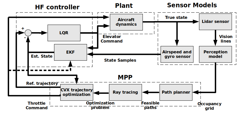
Figure 1: The system architecture, which consists of four components: the plant, sensor models, HF controller, and MPP. The plant simulates the dynamics of the vehicle. The sensor models are comprised of the lidar, airspeed and gyro sensors, and perception model. The HF controller regulates the system and also provides a high frequency estimate of the airspeed and angles for trajectory optimization at 100 Hz. MPP begins with planning a path from the occupancy grid, which is then used to determine constraints on an optimization problem through raytracing, and finally that problem is solved to find the trajectory.

II System Mode

Our system architecture is shown in Fig. 1. We discuss our plant and dynamics in Aircraft Dynamics Model subsection. The High Frequency (HF) controller operates on information provided by the airspeed and gyro sensors to regulate the vehicle, which is discussed in the High Frequency Controller subsection. The lidar sensor model provides information about nearby obstacles which is refined in to an occupancy grid in the perception model and this function is discussed in the perception model subsection. This overall structure is inspired by Ryll et al. [5].

II-A Aircraft Dynamics Model

We use a longitudinal flight dynamics model, with states being the downrange distance, vertical height, airspeed, pitch, pitch derivative, and flight path angle $(x,z,v,\theta,\dot{\theta},\gamma)$ [6].

The dynamics are:

$$\dot{x} =v\cos{\gamma}$$

$$\dot{z} =-v\sin{\gamma}$$

$$\dot{v} =-\frac{D}{m}-g\sin{\gamma}+\frac{T}{m}\cos{\alpha}$$

$$\ddot{\theta} =\frac{1}{I_{yy}}\mathcal{M}$$

$$\dot{\gamma} =\frac{L}{mv}-\frac{1}{v}\cos{\gamma}-\frac{T}{mv}\sin{\alpha}$$

The angle of attack ($\alpha:=\theta-\gamma$) is defined as the angle between the wings and oncoming airflow. The vehicle has two control inputs, the thrust ($T$) and elevator deflection ($\delta_{e}$ appearing in $\mathcal{M}$). Drag ($D$), lift ($L$), and moment ($\mathcal{M}$) are aerodynamic terms that depend on fixed aerodynamic coefficients and dynamic pressure, which is quadratic in terms of the airspeed. Full equations are given in the appendix. Mass ($m$), moment of inertia $I_{yy}$, and gravity ($g$) are also fixed parameters. We modeled our system as having airspeed and gyro sensors which provide measurements of airspeed and pitch, respectively, each with Normal errors. We assume the system is perfectly identified. Fig. 2 is a diagram of the modeled forces and angles.

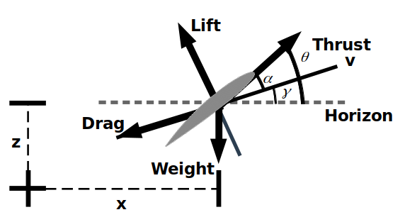
Figure 2: A free body diagram of forces acting on the system. $\gamma$, the flight path angle, is defined as the angle between velocity and the horizon. $\alpha$, the angle of attack, is defined as the angle between the wings (or thrust vector) and velocity. $\theta$, the pitch, is the angle between the wings (or thrust vector) and the horizon.

II-B High Frequency Controller

The HF controller consists of a Linear Quadratic Regulator (LQR) and an Extended Kalman Filter (EKF). The LQR regulates the flight path angle response of the system using elevator action, added to the feedfoward elevator signal determined by the planner. We linearize around straight and level flight conditions. The flight controller is responsible for tracking the desired pitch angle determined by the CVX Trajectory Optimization. CVX here refers to the convex optimization package [7], [8]. The Q matrix for state cost and R matrix for control cost are:

$$x_{ctrl}=\begin{bmatrix}v\\ \theta\\ \dot{\theta}\\ \gamma\end{bmatrix}\quad Q=\begin{bmatrix}10&0&0&0\\ 0&10&0&0\\ 0&0&0&0\\ 0&0&0&10000\end{bmatrix}\quad R=\begin{bmatrix}5\end{bmatrix}$$

The regulation of flight path angle is crucial for obstacle avoidance. The controller significantly improves the step response of the system. This control loop does not attempt to correct for positional error, which is only considered in the planner. We used the continuous time LQR solver from the Python Control Systems Library to calculate our LQR gains [9].

The EKF estimates the true states based on pitch and airspeed indicator measurements. The estimated state is used both in the flight controller and trajectory generation.

II-C Perception model

We modeled our perception system using a generated obstacle field and simulated lidar. The model identified objects at a particular angle and range with an error proportional to the range. These ray measurements are convert into an occupancy grid. This finds the $(x,y)$ coordinates where the lidar rays intersect with the obstacles in the field of view. The first pane of Fig. 3 shows the output occupancy grid from the perception model.

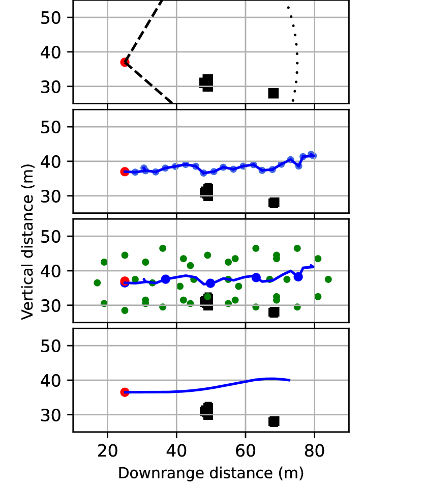
Figure 3: The MPP trajectory creation process, beginning with the first pane showing a lidar used to create an occupancy grid. This occupancy grid is used in the second pane to produce a feasible path with an RRT. The third shows raytracing around the path. The final pane shows a trajectory produced using the optimization problem from raytracing.

III Algorithm

Pseudocode for the MPP algorithm is given in Algorithm 1. The inputs to this method are an estimated dynamic state and occupancy grid, supplied by the EKF and perception model respectively. The path planner, a variation on RRT discussed in Section III-A, takes in the occupancy grid and identifies paths through this space towards the goal states of 54 meters directly ahead. The raytracing procedure converts these paths and the occupancy grid to convex optimization constraint and is discussed in Section III-B. The resulting optimization problem is solved in CVX, which is discussed in Section III-C. Fig. 3 shows the algorithm run with a single path. Because any given path determined by path planning may correspond to an infeasible well, we optimize several paths rather than a single one. This approach is shown in Fig. 5.

Algorithm 1 Model Predictive Planning

$x_{0}\leftarrow$ EKF

OccupancyGrid $\leftarrow$ PerceptionModel

Paths $\leftarrow$ RRT^∗-AR(OccupancyGrid)

Trajectory^∗

for Path in Paths do

     PositionConstraints $\leftarrow$ Raytrace(Path, OG)

     Trajectory $\leftarrow$ CVX($x_{0}$, PositionConstraints)

     Trajectory^∗ $\leftarrow$ mincost(Trajectory, Trajectory^∗)

end for

III-A Path Planning

Path Planning is carried out with the RRT variant RRT*-AR, which differs from RRT* in that it adds a cost penalty to close nodes sharing the same parent node [10]. This approach produces several suboptimal alternate routes to the goal. We found running RRT*-AR a single time provided insufficient dispersion of paths, but that sufficient dispersion was achieved by rerunning RRT*-AR with a low number of samples each time. The results of a single run are shown in the second pane of Fig. 3 and for 50 sampled paths in second pane of Fig. 5.

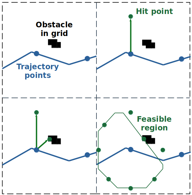
Figure 4: A visualization of raytracing. Trajectory points are determined from the path. 8 directions are searched from each of these to find if any obstacles are within a given search radius. Each hit point defines a linear constraint within which the final trajectory reference point can move.

III-B Raytracing

The raytracing procedure determines a feasible region around a path in which to search for a trajectory. While the optimization problem over the whole space is not convex, this local search problem is convex and thus much more practical to solve online. Our approach is inspired by the algorithm from Meerpohi et al. [11].

Beginning from points on the path, we check the occupancy grid (stored as a binary matrix) along 8 directions, returning when an occupied point is encountered. This process is visualized in Fig. 4. Hit points are shown in the third pane of Fig. 3. Hit points are translated to their position in a linearized straight and level vehicle frame and then an inner product is taken with the search direction, resulting in a linear constraint. Note, these constraints are padded slightly to account for rounding error and provide margin for tracking.

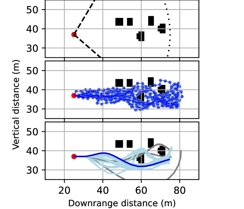
Figure 5: A visualization of the multi-trajectory process. It begins with the same lidar and path planning process, but many paths are planned instead of a single one. Each of these candidate paths is refined into a trajectory, with blue being the global optimal solution, light blue the suboptimal solutions, and gray infeasible results.

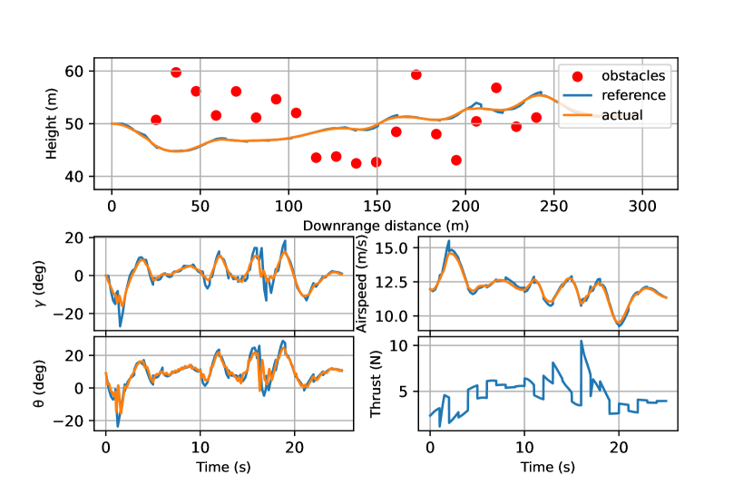
Figure 6: A full run of MPP with 20 obstacles and 25 paths per iteration is shown above. The reference command here is re-planned each second with a 4.5 second time horizon and orange shows the true trajectory.

III-C Trajectory Optimization

The trajectory optimization problem is a quadratic program. This approach to trajectory optimization is a form of convex optimization, an introduction to which is given by Malyuta et al. [12]. We make use of CVX to solve the quadratic program [7, 8]. The problem consists of the search variable ($\bar{x}$) which is the perturbation of states and controls from straight and level flight, the quadratic cost (Q), the equality constraint from the dynamics $\bar{A}$ which are equal to zero so that the dynamics are satisfied $(\bar{b})$, the inequality constraint matrix to capture the search directions $\bar{G}$, and its corresponding vector from raytracing $\bar{h}$. The optimization problem is:

$$\min(\bar{x}^{T}Q\bar{x})\quad\text{s.t.}\quad\bar{A}\bar{x}=\bar{b},\,\,\,\,\bar{G}x\leq\bar{h}$$

The system is linearized around straight and level flight. Those dynamics are captured in equality constraints:

$$\begin{split}\bar{x}=\begin{bmatrix}\delta x_{0}\\ \delta u_{0}\\ \vdots\\ \delta x_{n}\end{bmatrix}\quad\bar{A}=\begin{bmatrix}I&0&0&\cdots&0\\ A&B&-I&\cdots&0\\ \vdots&\ddots&\ddots&\ddots&\vdots\\ 0&\cdots&A&B&-I\end{bmatrix}\quad\bar{b}=0\end{split}$$

The feasible region found from raytracing is encoded as inequality constraints. The unit length search directions (g), of which there are p, are identical for each point and form into the blocks (G) that compose the inequality constraint matrix ($\bar{G}$):

$$\begin{split}G=\begin{bmatrix}g_{1}^{T}\\ \vdots\\ g_{p}^{T}\end{bmatrix}\quad\bar{G}=\begin{bmatrix}G&\cdots&0\\ \vdots&\ddots&\vdots\\ 0&\cdots&G\end{bmatrix}\\ \end{split}$$

For the experiments in this paper, $p=8$ gave good performance.

The raytracing vector is calculated by taking the inner product of the ”hit” point (o) and the search direction. The inner product of the new reference coordinate and the search direction must be less than this value of the coordinate to be inside the open region.

$$\begin{split}h_{i}=\begin{bmatrix}g_{0}^{T}o_{i0}\\ \vdots\\ g_{p}^{T}o_{ip}\end{bmatrix}\quad\bar{h}=\begin{bmatrix}h_{0}\\ \vdots\\ h_{n}\end{bmatrix}\end{split}$$

An additional inequality constraint is used to capture the throttle lower limit and prevent the command from falling below zero.

The cost function consists of a penalty on the control and the terminal state’s deviations from straight and level flight values. Experimentally, we determined that penalizing throttle greater than elevator produced smooth trajectories. Similarly, the final state weight of $w=100$ is based on experimentation. Obstacle avoidance is enforced solely in the constraints and does not appear in the cost function.

$$\bar{Q}=\begin{bmatrix}\begin{bmatrix}0_{6\times 6}&0_{6\times 2}\\ 0_{2\times 6}&C_{ctrl}\end{bmatrix}&\ldots&0_{8\times 8}&0_{8\times 2}\\ \vdots&\ddots&\vdots&\vdots\\ 0_{8\times 8}&\ldots&\begin{bmatrix}0_{6\times 6}&0_{6\times 2}\\ 0_{2\times 6}&C_{ctrl}\end{bmatrix}&0_{8\times 2}\\ 0_{2\times 8}&\ldots&0_{2\times 8}&wI_{2}\end{bmatrix}$$

$$\begin{split}C_{ctrl}=\begin{bmatrix}1&0\\ 0&3\end{bmatrix}\quad w=100\end{split}$$

III-D Dynamic modifications

Trajectory optimization is conducted using a time resolution of 0.25 seconds. However, this resolution is inadequate for accurately capturing the rotational dynamics exhibited by the system. To address this limitation, we introduced adjustments to the equality constraints associated with the rotational states. The differential equations are transformed into algebraic ones, constraining these states to their steady-state values after oscillations have decayed. In scenarios involving a single variable, this transformation takes on the following structure:

$$x_{t+1}=Ax_{t}+Bu_{t}\implies(I-A)x_{t+1}=Bu_{t}$$

In the optimization equations, this takes the form:

$$\bar{A}_{i}=\begin{bmatrix}0&\cdots&0&B&(I-A)&0&\cdots&0\end{bmatrix}$$

In addition to allowing the planner to be run at a lower resolution, this procedure also prevents negative interactions between the HF controller and feedfoward control from the LF planner.

IV Results

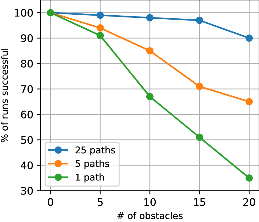
Figure 7: The MPP success rate base on number of paths and number of obstacles. With only a single path, the success rate is 35% in a cluttered environment but increases significantly to 90% given 25 paths. The case of a single path is representative of traditional MPC performance on this problem.

Fig. 6 shows an example run of MPP with 25 path candidates at each iteration through a field of 20 1-m radius obstacles. The vehicle’s vision is limited to 45 m ahead and it cruises at 12 m/s. The trajectory is planned 54 meters and 4.5 seconds ahead of the vehicle each iteration. The reference trajectory and open loop commands is calculated once per seconds, while the controller and dynamics resolve at 100 Hz.

Fig. 7 shows the performance of MPP based on numbers of paths and obstacles. Failure occurs if either an extreme state is reached (pitch exceed 60 degrees or flight path angle exceeding 45 degrees) or there is a collision with an obstacle. For a single path, the algorithm fails frequently when there are obstacles as often the path determined by the RRT does not correspond to a feasible trajectory. This high failure rate is representative of naive application of MPC to navigating an obstacle field. The success rate increases significantly when many paths are used. The tradeoff for this higher success rate is greater computational load. Each path takes approximately 0.04 seconds to refine on a Ryzen 9 4900HS processor, which precludes real time use with more than a small number of paths. The driver of computational load is raytracing, followed distantly by the optimization problem.

V Conclusion

MPP is a modification of traditional MPC to plan trajectories around obstacles. This approach is based on planning many paths around obstacles, raytracing around these paths to set up inequality constraints in a quadratic program, capturing dynamic constraints from an algebraic-differential equation as equality constraint, and solving this program repeatedly to re-plan around newly identified obstacles.

MPP is demonstrated in maneuvering around dense obstacle fields. MPP performance improves markedly with increasing numbers of paths, showing the need for many alternative paths to initialize the convex optimization in order to avoid problems of local in-feasibility.

We envision many promising avenues for advancing the MPP algorithm. The RRT*-AR path planner demands further refinement. A method producing 5-10 topologically distinct routes would not only improve the results of trajectory optimization but also reduce the computational load compared with the current approach. An alternative collocation methods to Euler collocation may also improve the reference trajectory. The raytracing method, which is the primary computational bottleneck, offers room for improvement. Furthermore, aspects of the stack, such as the simplistic approach to for obstacle grid generation, could be refined and provide additional criterion for selecting the new reference trajectory. The core MPP approach of iteratively refining path planning outcomes is a promising direction for future research.

VI Appendix

The coefficients of lift, drag, and pitching moment are modeled as functions of parameters of the angle of attack ($\alpha:=\theta-\gamma$) defined as:

$$\begin{split}C_{L}&=C_{L0}+C_{L\alpha}\alpha\\ C_{D}&=C_{D0}+KC_{L}^{2}\\ C_{\mathcal{M}}&=C_{\mathcal{M}0}+C_{\mathcal{M}\alpha}\alpha+C_{\mathcal{M}\dot{\alpha}}\dot{\alpha}+C_{\mathcal{M}\delta_{e}}\delta_{e}\end{split}$$

The above terms are mostly parameters: coefficient of lift at zero angle of attack ($C_{L0}$), coefficient of lift with angle of attack ($C_{L\alpha}$), coefficient of drag at zero angle of attack ($C_{d0}$), drag polar (K), coefficient of moment at zero angle of attack ($C_{\mathcal{M}0}$), coefficient of moment with angle of attack derivative ($C_{\mathcal{M}\dot{\alpha}}\dot{\alpha}$), and coefficient of moment with elevator ($C_{\mathcal{M}\delta_{e}}$).

The lift force, drag force, and pitching moment:

$$\begin{split}L=\frac{1}{2}\rho v^{2}SC_{L}\quad D=\frac{1}{2}\rho v^{2}SC_{D}\quad\mathcal{M}=\frac{1}{2}\rho v^{2}ScC_{\mathcal{M}}\end{split}$$

Here, S is the surface area of the wing, c is the chord length, and $\rho$ is the density of air.

The parameters used in the simulations in this paper are:

$$m =3.2\,\text{kg} C_{L\alpha} =5.73\,\frac{1}{\text{rad}} C_{L0} =0.5$$

$$K =0.05 C_{\mathcal{M}\alpha} =-8.02\,\frac{1}{\text{rad}} C_{\mathcal{M}0} =0.5$$

$$S =0.25\,\text{m}^{2} C_{\mathcal{M}\dot{\alpha}} =-0.46\,\frac{\text{s}}{\text{rad}} C_{\mathcal{M}\delta_{e}} =0.2$$

$$c =0.13\,\text{m} \rho =1.225\,\frac{\text{kg}}{\text{m}^{3}} C_{D0} =0.1$$

$$g =9.81\,\frac{\text{m}}{\text{s}^{2}} I_{yy} =0.17\,\text{kg}\,\text{m}^{2}$$

References

- [1] M. A. Patterson and A. V. Rao, “GPOPS-II: A MATLAB software for solving multiple-phase optimal control problems using hp-adaptive gaussian quadrature collocation methods and sparse nonlinear programming,” ACM Transactions on Mathematical Software (TOMS), vol. 41, no. 1, pp. 1–37, 2014.
- [2] P. E. Rutquist and M. M. Edvall, “PROPT-Matlab optimal control software,” Tomlab Optimization Inc, vol. 260, no. 1, p. 12, 2010.
- [3] J. H. Lee, “Model predictive control: Review of the three decades of development,” International Journal of Control, Automation and Systems, vol. 9, pp. 415–424, 2011.
- [4] S. Karaman and E. Frazzoli, “Sampling-based algorithms for optimal motion planning,” International Journal of Robotics Research, vol. 30, no. 7, pp. 846–894, 2011.
- [5] M. Ryll, J. Ware, J. Carter, and N. Roy, “Efficient trajectory planning for high speed flight in unknown environments,” in IEEE International Conference on Robotics and Automation (ICRA), 2019, pp. 732–738.
- [6] R. F. Stengel, “Longitudinal motions,” in Flight Dynamics. Princeton University Press, 2005, ch. 5.
- [7] M. Grant and S. Boyd, “CVX: Matlab software for disciplined convex programming, version 2.1,” http://cvxr.com/cvx, Mar. 2014.
- [8] ——, “Graph implementations for nonsmooth convex programs,” in Recent Advances in Learning and Control, ser. Lecture Notes in Control and Information Sciences, V. Blondel, S. Boyd, and H. Kimura, Eds. Springer-Verlag Limited, 2008, pp. 95–110, http://stanford.edu/~boyd/graph_dcp.html.
- [9] S. Fuller, B. Greiner, J. Moore, R. Murray, R. van Paassen, and R. Yorke, “The python control systems library (python-control),” in IEEE Conference on Decision and Control (CDC), 2021, pp. 4875–4881.
- [10] S. Choudhury, S. Scherer, and S. Singh, “RRT*-AR: Sampling-based alternate routes planning with applications to autonomous emergency landing of a helicopter,” in IEEE International Conference on Robotics and Automation (ICRA), 2013, pp. 3947–3952.
- [11] C. Meerpohl, M. Rick, and C. Büskens, “Free-space polygon creation based on occupancy grid maps for trajectory optimization methods,” IFAC-PapersOnLine, vol. 52, no. 8, pp. 368–374, 2019, 10th IFAC Symposium on Intelligent Autonomous Vehicles.
- [12] D. Malyuta, T. P. Reynolds, M. Szmuk, T. Lew, R. Bonalli, M. Pavone, and B. Açıkmeşe, “Convex optimization for trajectory generation: A tutorial on generating dynamically feasible trajectories reliably and efficiently,” IEEE Control Systems Magazine, vol. 42, no. 5, pp. 40–113, 2022.