Angular Correlation Function from sample covariance with BOSS and eBOSS LRG

Abstract

The Baryon Acoustic Oscillations (BAO) are one of the most used probes to understand the accelerated expansion of the Universe. Traditional methods rely on fiducial model information within their statistical analysis, which may be a problem when constraining different families of models. The aim of this work is to provide a method that constrains $\theta_{BAO}$ through a model-independent and compare parameter estimation of the angular correlation function polynomial approach, using the covariance matrix from the galaxy sample from thin redshift bins, with the usual mock sample covariance matrix. We proposed a different approach to finding the BAO angular feature revisiting previous work in the literature, we take the bias between the correlation function between the bins and the whole sample. We used widths of $\delta z=0.002$ separation for all samples as the basis for a sample covariance matrix weighted by the statistical importance of the redshift bin. We propose a different weighting scheme based only on random pair counting. We also propose an alternate shift parameter based only on the data. Each sample belongs to the Sloan Digital Sky Survey Luminous Red Galaxies (LRG): BOSS1, BOSS2, and eBOSS, with effective redshift $z_{eff}$: 0.35, 0.51, 0.71, respectively, and different numbers of bins with 50, 100, and 200 respectively. In addition, we correct the angular separation from the polynomial fit ($\theta_{fit}$) that encodes the BAO feature with a bias function obtained by comparing each bin correlation function with the correlation function of the whole set. We also tested the same correction choosing the bin at $z_{eff}$ and found that for eBOSS $\theta_{BAO}$ is in $1\sigma$ agreement with the Planck 18 model. BOSS1 and BOSS2 $\theta_{BAO}$ agreed in $1\sigma$ with the Pantheon+ & S$H_{0}$ES Flat$\Lambda$CDM model, in tension with Planck 18.

Keywords cosmology  $\cdot$ observations  $\cdot$ surveys  $\cdot$ large-scale structure of Universe  $\cdot$ BAO

1 Introduction

The Baryon Acoustic Oscillations (BAO) are one of the most used probes to understand the accelerated expansion of the Universe. Cosmological information can be extracted through the two-point correlation function and power spectra estimated with the sky distribution and redshift of standard tracers Peebles (2001). Among the tracers, the most used are the luminous red galaxy (LRG) first used by Eisenstein et al. (2005) and Percival et al. (2001). Now, a multi-tracer analysis is possible with emission line galaxies (Wang et al., 2020; De Mattia et al., 2021), quasars Hou et al. (2021) and Lyman-$\alpha$ forests (Des Bourboux et al., 2020).

Future and current surveys will reach a larger number of observed objects, such as the Dark Energy Spectroscopic Instrument (DESI) Flaugher & Bebek (2014), the Dark Energy Survey (DES) Rosell et al. (2022), the Large Synoptic Survey Telescope (LSST) surveyAnsari et al. (2019), the Javalambre-Physics of the Accelerated Universe Astrophysical Survey (J-PAS) (Benitez et al., 2014), Euclid (Scaramella et al., 2022). Larger samples have the advantage of being statistically robust and less susceptible to cosmic variance (Moster et al., 2011). Their goal is to reach higher precision in order to test different cosmological models. This is only achievable through a template analysis that can be applied to any model.

The traditional methods rely on fiducial cosmology and ad hoc parameters to fix nonlinear effects (Seo et al., 2008). Moreover, the statistical analysis carries fiducial model information within its template. A possible issue with these methods is the applicability to test other families of models. Anselmi et al. (2016); Anselmi et al. (2018) proposed a method to find the BAO peak without a fiducial model and avoid nonlinear interference. Sánchez et al. (2011, 2013) analysed the angular and radial correlation functions using a polynomial fit, also independent of the model. Marra & Chirinos Isidro (2019) and Menote & Marra (2022) followed this construction using the Sloan Digital Sky Server (SDSS) precise surveys.

Parameter estimation from Large Scale Structure (LSS) galaxy counting requires a covariance matrix. Usually, the community uses hundreds of mock catalogs that mimic surveys. This can be done by N-body simulations such as the MultiDark-Patchy Mocks by (Kitaura et al., 2016; Rodríguez-Torres et al., 2016), and the N-body Parallel Particle-Mesh GLAM code (PPMGLAM) by Klypin & Prada (2018), which is the core of GLAM (GaLAxy Mocks). Simulation mocks are highly computationally expensive because they solve the matter density field evolution. The solution for many collaborations was to use a modest mock construction like the Log-Normal mocks, that can be found in CoLoRe (Ramírez-Pérez et al., 2022), FLASK (Xavier et al., 2016), nbodykit (Hand et al., 2018) LogNormalCatalog. Both approaches require fiducial cosmology, something that would be desirable to avoid.

Scranton et al. (2002) estimated the covariance matrix assuming that the error distribution is Gaussian. Zehavi et al. (2002, 2004) used the so-called jackknife error estimate, by dividing a larger sample into subsamples in order to find the covariance matrix. Their analysis concluded that the results were representative error estimators. Ross et al. (2007) also used subsamples to find the covariance matrix and error bars from the data set. However, there was a lack of observed objects. The latest data sets from spectroscopic surveys must provide even more representative errors and covariance matrices once we are provided with more objects, thus thinner redshift subsamples.

The aim of this work is to provide a pipeline to constrain $\theta_{BAO}$ through a model-independent estimation of the angular correlation function. We use thin bins of redshift with width $\delta z=0.002$ as the basis for a covariance matrix weighted by the statistical importance of the redshift bin. Our analysis compares the sample covariance to the covariance matrix originating from mock catalogs. We compare samples with different effective redshift values, from lowest $z$ to highest $z$ and check the consistency according to each scale. Furthermore, we correct the angular separation that encodes the BAO feature of the Sánchez et al. (2011) polynomial fit by a bias function that compares the correlation function of each bin with the whole set.

Our analysis is first structured with our methodology in 2 where we describe the data used in 2.1, how it was divided into redshift bins in 2.2, and finally its correlation function estimator in 2.3. Next, we describe the construction of the covariance matrix with the data and with mocks in 3. The polynomial function is described in 4.2 and our $\theta_{BAO}$ method in section 3.2. The results and conclusion are found in 4 and 5, respectively.

2 Methods

2.1 Data and mocks

In this work, we used two data sets from the SDSS. The LRG and the LRG CMASS data from the Data Release 16 (DR16) Wang et al. (2020) of the extended Baryon Oscillation Spectroscopic Survey (eBOSS) spectroscopic observations from the SDSS IV. The sample is distributed in both Northern Galactic Cap (NGC) and Southern Galactic Cap (SGC) with a redshift range of $0.6\leq z\leq 1.0$ and a total of $552,274$ galaxies. Its random catalogue contains fifty times more galaxies than the real one.

The other set consists of galaxies from the BOSS sample of the SDSS-III DR12. We separated a redshift range $0.3\leq z<0.4$ called the BOSS1 set and BOSS2 range is $0.4\leq z<0.6$. The summary of the data specification can be found in Table 1. We chose this minimum redshift because, according to our tests, smaller redshift ranges did not show a significant signal for the BAO feature, as expected.

For the eBOSS set, we used $N=1,000$ realisations of realistic mocks catalogs from Zhao et al. (2021), for each galactic cap, based on the effective Zel’dovich approximation mock generator (EZmock) by Chuang et al. (2015). The mocks were constructed using the Zel’dovich approximation Zel’Dovich (1970) which is faster than producing mocks using N-body simulations and accurate in clustering statistics.

We used $N=1,000$ realisations of the MultiDark-Patchy mocks for the BOSS set. The mocks were constructed for both the LOWZ redshift range Kitaura et al. (2016) and the CMASS part Rodríguez-Torres et al. (2016).

We cut the mocks to match the survey’s redshift range. The same routine was applied to calculate the angular correlation function for the mocks using the same random catalogue for all mocks.

2.2 Redshift bins

In order to get a direct BAO measurement, we used an approach similar to the one developed by Sánchez et al. (2011).

eBOSS sample was divided into 200 redshift bins with width $\delta z=0.002$. The choice was made considering the distribution of galaxies in the sky. One wants many bins to construct a fair covariance matrix and enough galaxies in each bin to get the BAO feature through angular counting. The angular pairs of each bin were computed using the code corrfunc developed by Sinha & Garrison (2020). The data-data ($DD$), the data-random ($DR$), and random-random ($RR$) pairs counts calculated for angular pixels from $0.8^{\circ}$ to $10^{\circ}$ with width $\delta\theta\sim 0.4^{\circ}$. This was also a convenient choice to find the BAO feature. Larger angles would provide a smeared function, while smaller ones would have too few galaxies.

The BOSS1 set was divided into 50 bins with width $\delta z=0.002$, angular range $1^{\circ}<\theta<12^{\circ}$ with $\delta\theta\sim 0.31^{\circ}$. BOSS2 was divided into 100 bins with the same redshift separation and the same angular configuration as eBOSS. The redshift distribution for the chosen binning can be visualized in Figure 1.

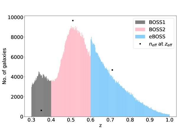
Figure 1: Each sample bin separation. The black squares are the $n_{eff}$ of each sample. BOSS1, BOSS2, and eBOSS are in gray, pink, and blue, respectively.

With the pairs counts, we computed the angular two-point correlation function for each redshift bin using the Landy-Szalay estimator Landy & Szalay (1993). Each angular function was normalised according to its corresponding i-th bin length. The angular correlation function ($\mathrm{w}_{i}$) of the i-th bin is written in the following equation:

$$\mathrm{w}_{i}(\theta)=\left(\frac{N_{i,rand}}{N_{i,data}}\right)^{2}\frac{DD_{i}(\theta)}{RR_{i}(\theta)}-2\frac{N_{i,rand}}{N_{i,data}}\frac{DR_{i}(\theta)}{RR_{i}(\theta)}+1\text{ ,}$$ (1)

where $N_{i,rand}$ is the number of galaxies in the random bin, and $N_{i,data}$ in a data bin.

Table 1: Data specifications

Sample	$z$ range	No. of Galaxies	$z_{eff}$	No. of bins
BOSS1	$0.3\leq z<0.4$	$192,285$	$0.35$	$50$
BOSS2	$0.4\leq z<0.6$	$686,370$	$0.51$	$100$
eBOSS	$0.6\leq z\leq 1.0$	$552,274$	$0.71$	$200$

2.3 Weighting-scheme and correlation function

In addition to normalisation, it is important to account for the statistical significance of each bin. Our approach was to use the total weights ($w_{tot,\alpha}$) that account for the systematic effects of the spectrographs. For the LRG sample, the weights given by

$$w^{LRG}_{tot}=w_{sys,\alpha}\cdot w_{cp,\alpha}\cdot w_{noz,\alpha},$$ (2)

which is described in Gil-Marín et al. (2020). We used the prescription described in Reid et al. (2016) with the pCMASS, eBOSS and CMASS BOSS samples:

$$w_{tot,\alpha}=w_{sys,\alpha}(w_{cp,\alpha}+w_{noz,\alpha}-1),$$ (3)

where the total galaxy weights $w_{tot,\alpha}$ depends on the total angular systematic weights $w_{systot,\alpha}$, the weight for close pair correction $w_{cp,\alpha}$, and the total weight to the nearest neighbour of the redshift failure $w_{noz,\alpha}$. corrfunc (Sinha & Garrison, 2020) weights the pairs using the pair_product method, which is simply multiplying the weights of the galaxies in a pair.

We computed the effective redshift of the three samples according to the following equation based on Beutler et al. (2011):

$$z_{eff}=\frac{\displaystyle\displaystyle\sum_{\alpha<\beta}\frac{w_{\alpha}w_{\beta}(z_{\alpha}+z_{\beta})}{2}}{\displaystyle\displaystyle\sum_{\alpha<\beta}w_{\alpha}w_{\beta}}\text{ ,}$$ (4)

where $\alpha$ and $\beta$ represent galaxies in a sample, and $w_{\alpha|\beta}$ is their $w_{tot}$. The values are shown in Table 1.

Random and mock bins do not carry the systematic effects of fibres on the spectrographs. Since the available FKP weight by Feldman et al. (1993) accounts for the number of galaxies in a volume, we use unit weights $w=1.0$ for the angular correlation function.

As the bins have different sizes and redshifts, the bins also need to be weighted. For that, we consider a bin weighting revisiting Marra & Chirinos Isidro (2019). Now, redshift bins are weighted instead of pixels.

The weighting of each bin is similar to the variance of the weights of each random galaxy. For each bin, the weight $rr_{i}$ is written as:

$$rr_{i}=\frac{\left(\displaystyle\displaystyle\sum_{j}RR_{ij}\right)^{2}-\displaystyle\displaystyle\sum_{j}RR_{ij}^{2}}{2}$$ (5)

where $i$ stands for the redshift bin and $j$ for $j$-angular separation. Marra & Chirinos Isidro (2019) wrote $rr_{\alpha}$ as a weight for each pixel; here we use the pair counting $RR$ because all of them are uncorrelated with the observed points but still an accurate representation of them in terms of redshift. We want to weigh the bins according to statistical significance and that is related to how many galaxies are in the $ij$ box.

Finally, the correlation function $\mathrm{W}(\theta)$ is computed as a weighted mean of the functions for each bin

$$\mathrm{W}(\theta)=\frac{\displaystyle\displaystyle\sum\limits_{i}\mathrm{w}_{i}(\theta)\cdot rr_{i}}{\displaystyle\displaystyle\sum\limits_{i}rr_{i}}.$$ (6)

3 Covariance matrix and $\theta_{BAO}$

The whole sample has an effective number of galaxies per bin ($n_{eff}$):

$$n_{eff}=\frac{\left(\displaystyle\sum_{i}rr_{i}\right)^{2}}{\displaystyle\sum_{i}rr_{i}^{2}}.$$ (7)

We consider a good sample the one that has an $n_{eff}$ close to the number of galaxies at the $z_{i}\sim z_{eff}$. This can be seen in Figure 1, where we display the $n_{eff}$ of each sample as black squares. The BOSS2 and eBOSS present this characteristic, while the smaller sample with fewer bins shows disagreement with the size of the bin.

Equation (1) works as a matrix of many correlation function realisations, similar to the usual usage of mocks. We use each $\mathrm{w}_{i}(\theta)$ compared to $\mathrm{W}(\theta)$ from equation 6 to construct the sample covariance matrix $\zeta_{ml}$:

$$\zeta_{ml}=\frac{n_{eff}^{-1}}{(N_{i}-1)}\displaystyle\sum\limits_{i=1}^{N_{i}}[\mathrm{w}_{i}(\theta_{m})-\mathrm{W}(\theta_{m})]\times[\mathrm{w}_{i}(\theta_{l})-\mathrm{W}(\theta_{l})].$$ (8)

Basically, we compute the bias between each $\mathrm{w}_{i}(\theta)$ and $\mathrm{W}(\theta)$, but because $\mathrm{w}_{i}(\theta)$ is not weighted according to Eq. (3), so we must correct this by $n_{eff}$.

As means of comparison, we use mocks to compute $\mathrm{W}_{k}(\theta)$ of the $k$-mock and test the method. Now, the covariance matrix $C_{ml}$:

$$C_{ml}=\frac{n_{eff}^{-1}}{N-1}\displaystyle\sum\limits_{k=1}^{N=1000}[\mathrm{W}_{k}(\theta_{m})-\mathrm{\bar{W}}(\theta_{m})]\times[\mathrm{W}_{k}(\theta_{l})-\mathrm{\bar{W}}(\theta_{l})],$$ (9)

where $\mathrm{\bar{W}}$ is the average over the correlation function $W_{k}(\theta)$ of each mock. Nevertheless, Eq. (9) is not model-independent, because the mocks were constructed assuming a fiducial cosmology.

3.1 Polynomial function

We used Sánchez et al. (2011) expression below for the angular two-point correlation function to fit our estimated $W(\theta)$.

$$\mathcal{W}(\theta)=A+B\theta^{\gamma}+Ce^{-\frac{(\theta-\theta_{fit})^{2}}{2\sigma^{2}}}$$ (10)

The parameter $A$ is related to the behaviour of the function after the BAO peak. $B$ and $C$ weigh the importance of their respective terms, if there is no BAO peak, for instance, $C=0$. $\gamma$ is the power law of the function’s overall shape. The physical parameters are $\theta_{fit}$ and $\sigma$, $\theta_{fit}$ gives the position of the BAO, while $\sigma$ is the width of the BAO.

We applied Gaussian priors to the parameters that are related to the BAO: $C$, $\theta_{fit}$, and $\sigma$, the priors are written in table 2. The parameter estimation was done using the maximum likelihood estimator method through the emcee’s Affine Invariant Markov Chain Monte Carlo (MCMC) Ensemble sampler software by Foreman-Mackey et al. (2013). The fitting is done with the $W(\theta)$ from the data, we will compare the best-fit results alternating between $\zeta_{ml}$ and $C_{ml}$.

	$C$	$\theta_{fit}$	$\sigma$
BOSS1	$\mathcal{N}(5\times 10^{-3},1\times 10^{-5})$	$\mathcal{N}(6.00,0.01)$	$\mathcal{N}(1.00,0.01)$
BOSS2	$C>0$	$\mathcal{N}(4.2,0.1)$	$\mathcal{N}(0.04,0.01)$
eBOSS	$\mathcal{N}(7.60\times 10^{-3},1\times 10^{-5})$	$\mathcal{N}(2.70,0.01)$	$\sigma>0$

Table 2: Priors used in the MCMC, both with $\zeta_{ml}$ and $C_{ml}$.

The chi-squared function is:

$$\chi^{2}=\displaystyle\sum\limits_{ml}\left[\mathrm{W}(\theta_{m})-\mathcal{W}(\theta_{m})\right]\zeta_{ml}^{-1}\left[\mathrm{W}(\theta_{l})-\mathcal{W}(\theta_{l})\right],$$ (11)

the same equation is used with $C_{ml}$.

3.2 The BAO scale $\theta_{BAO}$

Should the estimator and its covariance matrix be representative of the angular pairs counting of the LSS, we can constrain cosmological parameters from fitting a model to the data. For that we need to find the BAO signal, $\theta_{BAO}$ as a function of $\theta_{fit}$. Here, we will focus on the use of a totally model-independent procedure, leaving a model that gets the advantage of our estimator for future work.

We propose a similar method to Carvalho et al. (2016) to find $\theta_{BAO}$. We take the correlation function estimation for the whole set, as in Eq. (1) without weighting according to the random bins, to find $\mathrm{w}_{\delta z=0}(\theta)$ and compute a bias function, the difference between $\mathrm{w}_{\delta z=0}(\theta)$ and the $\mathrm{w}_{i}(\theta)$ not normalised by $rr_{i}$:

$$\Delta\mathrm{w}_{i}(\theta)=\frac{\mathrm{w}_{i}(\theta)-\mathrm{w}_{\delta z=0}(\theta)}{\sqrt{\int|\mathrm{w}_{i}(\theta)-\mathrm{w}_{\delta z=0}(\theta)|^{2}\mathrm{d}\theta}},$$ (12)

where $\Delta w_{i}(\theta)$ is normalised by one. Next, we take this bias function and compute the 20^th percentile and the median over the bins to get our shift parameter $\alpha$ as a function of $\theta$:

$$\alpha_{20}(\theta)=\frac{\displaystyle\sum_{i}^{N_{20}}\Delta\mathrm{w}_{i}(\theta)}{N_{20}}\geq\frac{1}{5},$$ (13)

$$\alpha_{50}(\theta)=\frac{\displaystyle\sum_{i}^{N_{50}}\Delta\mathrm{w}_{i}(\theta)}{N_{50}}\geq\frac{1}{2}.$$ (14)

$\alpha_{20}(\theta)$ represents the bias function of a bin that is greater or equal to 20% of the bias function of the other bins, $\alpha_{50}(\theta)$ is 50% greater or equal to the other bias functions.

Finally, $\theta_{BAO}$ is the correction of the model-independent $\theta_{fit}$ according to the bias of each with respect to the correlation function if the binning was not applied:

$$\theta_{BAO}(z_{eff})=\theta_{fit}+\alpha(\theta_{fit})\theta_{fit}.$$ (15)

$\alpha(\theta_{fit})$ is the value of the function $\alpha$ at the angle found from the MCMC fitting results, both from sample covariance and mock covariance. We used $\alpha_{20}$ and $\alpha_{50}$ in Eq. (15) and will present the results for both.

We also tested $\alpha$ in equation (15) as the normalized dispersion between the whole set correlation function and the one for the bin which contains $z_{eff}$. This bin is expected to be representative of the whole sample as described in section 2.3. We can write it as

$$\alpha_{eff}(\theta)=\frac{\mathrm{w}_{eff}(\theta)-\mathrm{w}_{\delta z=0}(\theta)}{\sqrt{\int|\mathrm{w}_{eff}(\theta)-\mathrm{w}_{\delta z=0}(\theta)|^{2}\mathrm{d}\theta}},$$ (16)

4 Results

4.1 Covariance matrix

The correlation matrices of both mocks and data sets are shown in Fig. (2). The top left panel shows the correlation matrix of the BOSS1 sample, while the MultiDark Patchy Mocks results are shown on the top right one. Both plots show a higher correlation at smaller scales, from $\sim 1^{o}$ to $\sim 5^{o}$, and the data matrix is more noisy than the mocks, as one could expect.

In the middle left panel, we can see that BOSS2 has more low correlation patches when compared to BOSS1, possibly due to the bigger number of objects and depth of this sample. Its mock counterpart shows much less noise, as expected, and similar over-correlated regions on both extremes of the angular separation. Additionally, the BOSS2 sample shows a high correlation between small and big scales that is not visible in BOSS1 and the mocks.

Lastly, the results for eBOSS, the larger and deeper sample, are shown in the bottom panels of Fig (2). The data correlation matrix is clearly more noisy, and it does not show regions of stronger or weaker correlation, except for the diagonal. The EZ mocks appear to have a similar pattern to that of the other mocks, but there is a stronger correlation region on larger scales unlike the other mocks.

4.2 Polynomial fit

After taking the steps described in the previous section, we get the estimated correlation function, where the results of the physical parameters of the fitting formula are compiled in Table 3. The comparison between mock and data fitting is shown in figures 3, 4, and 5. The contour indicate the $68\%$, $95\%$, and $99.7\%$ confidence level regions, from darker to lighter colours, respectively.

Table 3: Best-fit parameters

Sample	$C$	$\theta_{fit}(^{o})$	$\sigma(^{o})$
BOSS1 using $\zeta_{ml}$	$0.010\pm 0.001$	$5.66\pm 0.02$	$0.15\pm 0.03$
BOSS1 using $C_{ml}$	$0.0047\pm 0.0001$	$5.79\pm 0.006$	$0.198\pm 0.005$
BOSS2 using $\zeta_{ml}$	$0.002\pm 0.0001$	$4.24\pm 0.02$	$0.30\pm 0.01$
BOSS2 using $C_{ml}$	$0.02\pm 0.01$	$4.21\pm 0.02$	$0.030\pm 0.009$
eBOSS using $\zeta_{ml}$	$0.008\pm 0.002$	$2.72\pm 0.09$	$0.13\pm 0.05$
eBOSS using $C_{ml}$	$0.009\pm 0.001$	$2.77\pm 0.04$	$0.12\pm 0.03$

We chose Gaussian priors for the physical parameters for all samples. But instead of using traditional random walkers, we used a mixture of moves in our code, in order to improve the performance of the MCMC walkers. 80% of the moves are a "differential evolution" algorithm Differential Evolution MCMC (DEMCMC) by Nelson et al. (2013), available in emcee as DEMove. The other 20% of the moves are done with KDEMove.

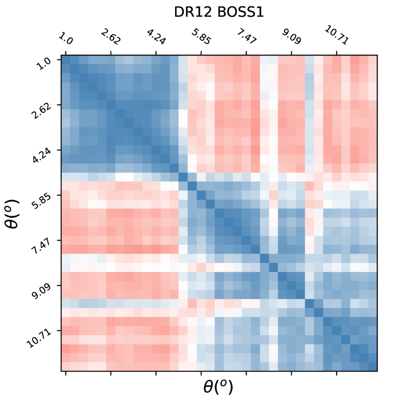
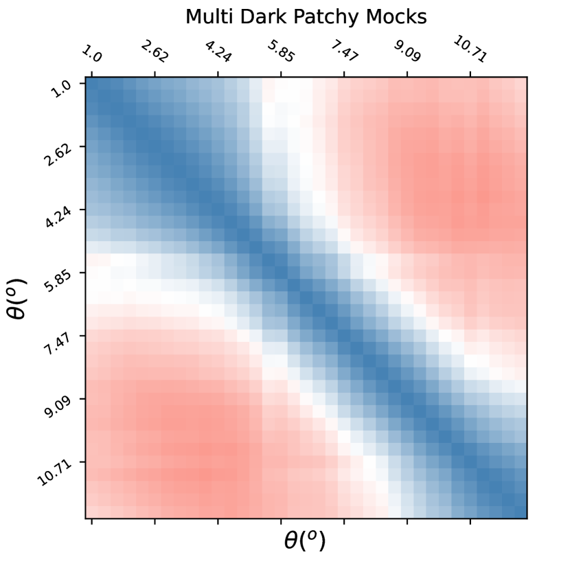
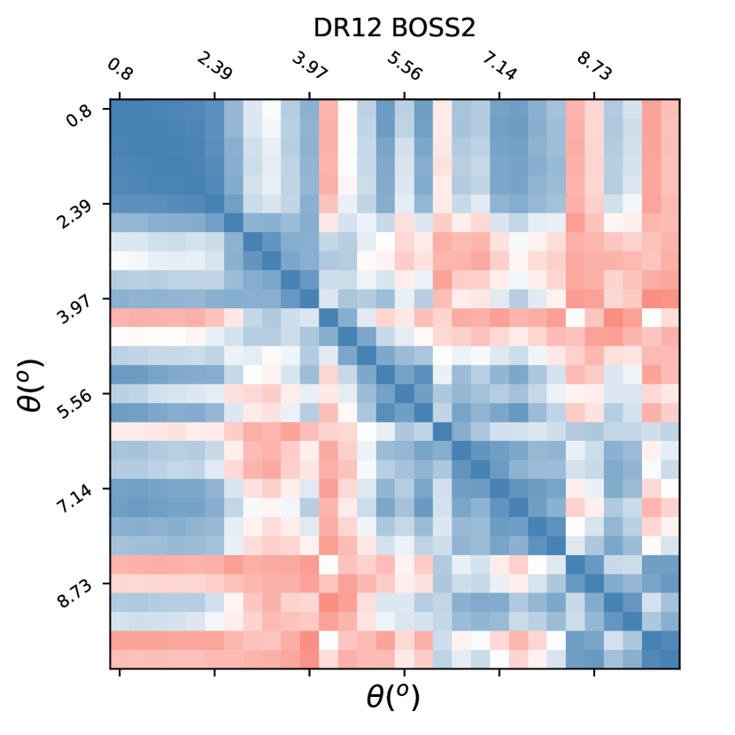
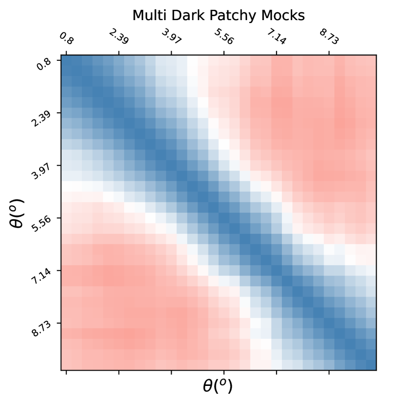
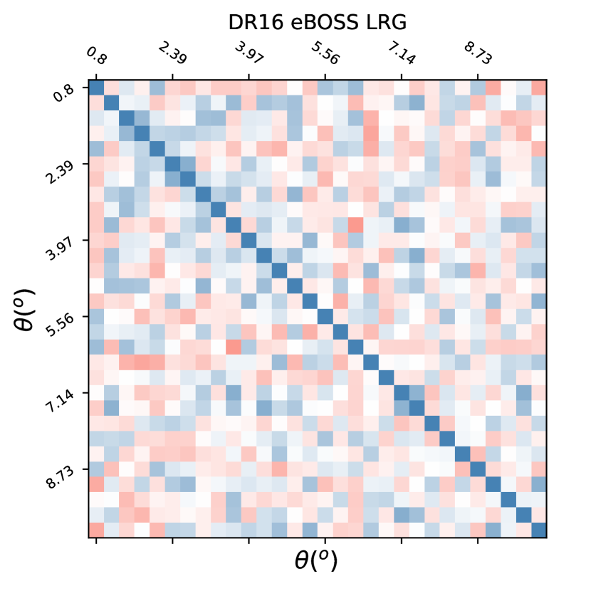
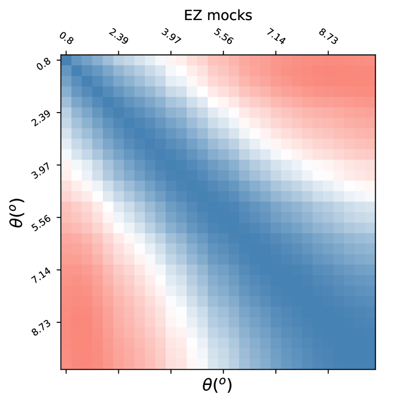
Figure 2: Correlation matrices relative to $\zeta_{ml}$, left column, and $C_{ml}$, right column. Negative correlation in salmon, a positive correlation in blue, and a zero correlation in white colour.

Table 2 shows the priors chosen for all cases. For all results shown in Figures 3, 4 and 5, and table 3, we used the real data and changed the covariance as indicated. BOSS1 and BOSS2 results for the parameter $C$ did not agree at $\sim 5\sigma$ when we change the covariance from data to their respective mocks, while eBOSS does not show such issue.

eBOSS agrees within $1\sigma$ compared to their respective mocks for all parameters, as seen in Figure 5, with the mocks covariance presenting tighter constraints as expected due to the lower noise. The posteriors are not close to a Gaussian distribution, showing a long tail towards higher values of $C$.

BOSS1 did not show the same behaviour; the main reason is the size of the sample. It is reasonable to expected that the mocks do not include all possible nonlinear effects of the real LSS. This should be particularly important for lower redshift samples, where such effects will be greater. The method used here does not account for this depth dependence. The struggles with lower redshift and modelled solutions have been discussed extensively in the literature, especially in the 3D power spectrum case as seen in Seo et al. (2008) and Xu et al. (2012).

We see in Figure 3 that, despite the tension in the results, both $C_{ml}$ and $\zeta_{ml}$ show the BAO feature, with tighter 1$\sigma$ CL for $C_{ml}$ results. The first sample is affected by two peculiarities. As a consequence, we expect that the precision of the angular diameter distance will be affected.

BOSS2 presented better results based on $\zeta_{ml}$ (Figure 4), while for $C_{ml}$ (Figure 4) we obtained broader posteriors. This again reflects that this method does not account for nonlinear effects and that the mocks are not perfect idealizations of the LSS.

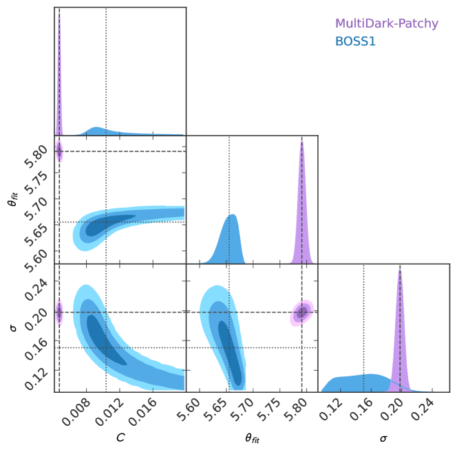
Figure 3: Comparison between results for the BOSS1 using using $\zeta_{ml}$ in blue, and $C_{ml}$ in purple, using pygtc (Bocquet & Carter, 2016) for the parameters $C$, $\theta_{fit}$, and $\sigma$.

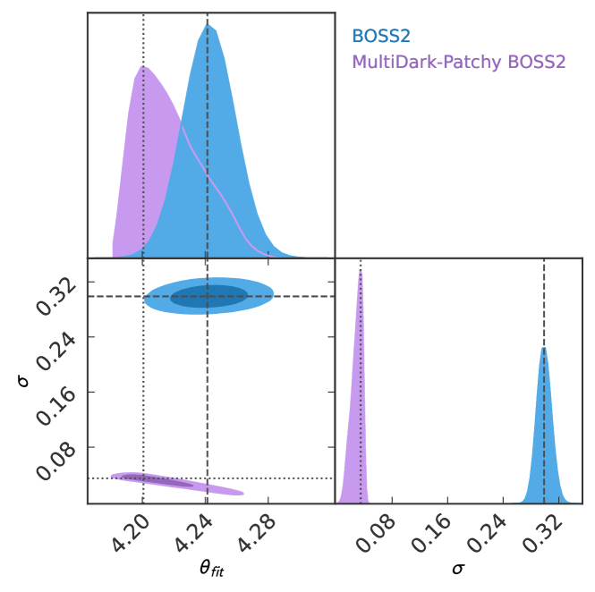
Figure 4: Comparison between results for the BOSS2 using using $\zeta_{ml}$ in blue, and $C_{ml}$ in purple, using pygtc (Bocquet & Carter, 2016) for the parameters $C$, $\theta_{fit}$, and $\sigma$.

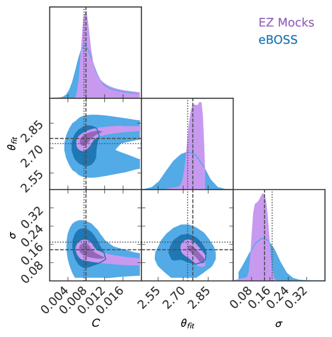
Figure 5: Comparison between results for the eBOSS using using $\zeta_{ml}$ in blue, and $C_{ml}$ in purple, using pygtc (Bocquet & Carter, 2016) for the parameters $C$, $\theta_{fit}$, and $\sigma$.

4.3 $\theta_{BAO}$ results

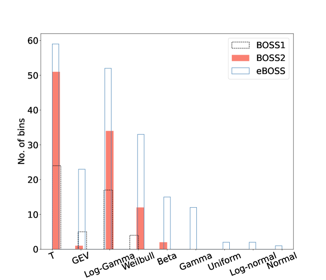
Figure 6: The best-fit of the types of distribution of the bias function $\Delta w_{i}(\theta)$ in terms of $\delta z$ for each sample. The shaded black bars are BOSS1 bins, the salmon shaded bars are BOSS2 bins, and the eBOSS bars are in blue bars.

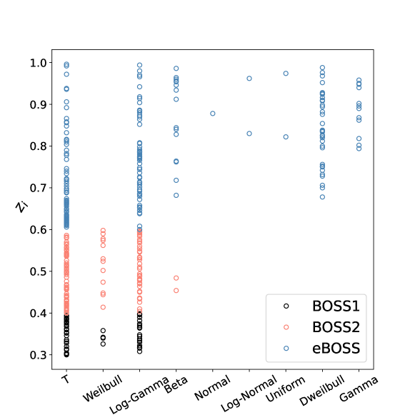
Figure 7: The the best-fit of the types of distribution of the bias function $\Delta w_{i}(\theta)$ in terms of $z_{i}$. The black, salmon, and blue circles represent BOSS1, BOSS2, and eBOSS bins, respectively.

The bias function from Eq. (12) can be visualized as a scatter matrix between the redshift bins. Some bin distributions can be found in Appendix A, in which we chose 10 bins close to the effective redshift to understand this bias relation. If the bias function is close to zero, the difference between the CFs of each bin and the whole set is supposed to be close to a symmetric distribution with mean zero. We fitted these distributions for some common analytic distribution functions using distifit (Taskesen, 2020) and show the best-fit in Figure (6). We see that eBOSS has more symmetric best-fit distributions (T, Uniform, Log-normal, Normal) in terms of $\delta z$ than the other samples. We show again in Figure (7) the best-fit distribution types, indicating the central redshift of each bin. We can see that most bins are symmetric for all samples. However, we see that there are many low-z bins ($z<0.5$) with Log-Gamma best-fit bias functions, with only $50$ (BOSS1) and $100$ (BOSS2) bins which reduces the statistical significance of our results. eBOSS, on the other hand, proves to be a reliable sample, with more symmetric bias functions compared to the others.

In Figure 8 we show the $\theta_{BAO}$ results from Eq. (15). The sample covariance results are shown in blue, while the mock covariance results are in salmon with two different cosmological parameter references to compare with our results. The first is the Planck 2018 Collaboration (Aghanim et al., 2020), which is shown in black with a gray-shaded region. We considered the TT, TE, EE+lowE+lensing constraints. The second model is based on the Pantheon+ & S$H_{0}$ES (Brout et al., 2022) Flat$\Lambda$CDM in light blue with a purple shaded region. The cosmological parameters can be found in Table 4. The shaded regions are the $68\%$ (darker) and $95\%$ (lighter) confidence levels (CL) for the results. The curves are plotted using the following relation as a function of redshift:

$$\theta_{BAO}=\frac{r_{s}}{(1+z)D_{A}(z)},$$ (17)

where $D_{A}(z)$ is the angular diameter distance as a function of redshift and $r_{s}=147.090\pm 0.026$ Mpc is the sound horizon at drag epoch which is the Planck 18 Aghanim et al. (2020) TT, TE, EE, lowE, lensing result for the black region. For S$H_{0}$ES fiducial model we chose to vary the sound horizon between the smaller and larger results from Planck 18 (Aghanim et al., 2020) including the BAO constraints, this gives $r_{s}=146.46\pm 2.32$ Mpc.

Parameters	Planck 18	Pantheon+ & S$H_{0}$ES
$\Omega_{m}$	$0.3153\pm 0.0073$	$0.334\pm 0.018$
$\Omega_{\Lambda}$	$0.6847\pm 0.0073$	$0.666\pm 0.018$
$H_{0}$(km s-1 Mpc-1)	$67.36\pm 0.54$	$73.6\pm 1.1$

Table 4: Parameters for Flat$\Lambda$CDM cosmology for Planck 18 (Aghanim et al., 2020) and Pantheon+ & S$H_{0}$ES (Brout et al., 2022).

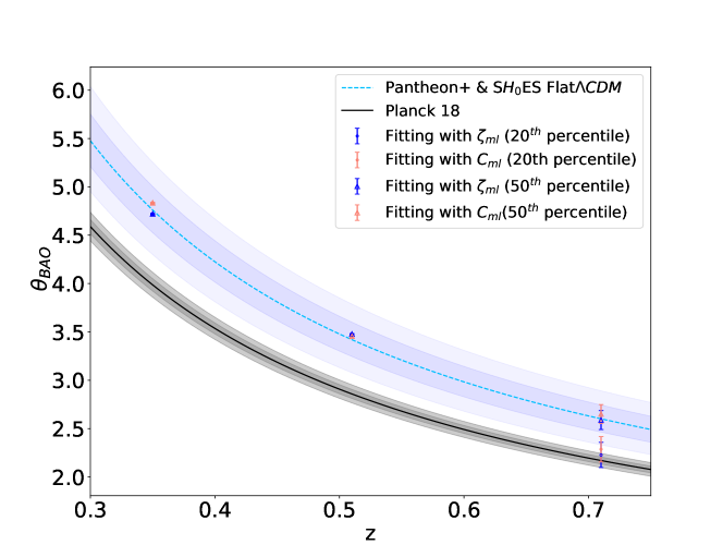
Figure 8: $\theta_{BAO}$ as a function of redshift with $\alpha$ from Eq. (13) and (14). Planck 18 (Aghanim et al., 2020) $\theta_{BAO}$ is shown as the black line and S$H_{0}$ES (Brout et al., 2022) as the dashed blue region. We kept the blue color for the results with $\zeta_{ml}$ and salmon for $C_{ml}$. The shaded regions are the CL of Planck 18 in gray and S$H_{0}$ES in purple, the darker region corresponds to 68% CL and the lighter one to 95% CL. The dots correspond to $\alpha_{20}(\theta)$ correction and the triangles correspond to the $\alpha_{50}(\theta)$ correction.

We see in Figure 8 that the highest $z_{eff}$ sample, eBOSS, has the larger error bars, this is due to the incompleteness of the sample. Since Eq. (6) weights the correlation function of each bin according to its random catalog size, this clearly affects $\theta_{fit}$ and consequently $\theta_{BAO}$, as the number of galaxies per bin decreases with redshift for eBOSS, so the $n_{eff}$ is smaller compared to the other samples which increase the error bars. For all samples, the mock results have smaller error bars due to a larger number of galaxies per bin. Since we chose the same bin size ($\delta z=0.002$) for all samples this results in fewer galaxies per bin for BOSS1 when compared to BOSS2 which leads to greater error bars for BOSS1.

The results for $\alpha_{20}$ agree with the ones from $\alpha_{50}$ in Figure 8 for BOSS1 and BOSS2, this indicates that $\Delta\mathrm{w}_{i}$ distribution is narrow. eBOSS, on the other hand, had a significant change, the reason for that again is the decline in the number of galaxies as $z_{i}$ increases. The comparison of $\theta_{BAO}$ between data and mock analysis is shown in Table 5.

	$\theta_{BAO}^{20}-\theta_{BAO}^{50}$	$\theta_{BAO}^{20}/\theta_{BAO}^{50}$
BOSS1	$-0.006$	$99.87\%$
BOSS2	$-0.002$	$99.93\%$
eBOSS	$-0.361$	$86.04\%$
BOSS1 mocks	$-0.006$	$99.87\%$
BOSS2 mocks	$-0.002$	$99.93\%$
eBOSS mocks	$-0.365$	$86.24\%$

Table 5: The difference between the 20^th percentile and the 50^th percentile.

All samples agree within the $68\%$ CL with Pantheon+ & S$H_{0}$ES, even for eBOSS. However, we must consider how BOSS1 is shallower than the other samples. In this sense, eBOSS is the most reliable sample, especially because $\zeta_{ml}$ was not as noisy as the other samples.

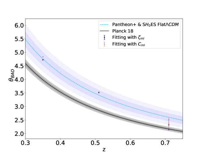
Figure 9: $\theta_{BAO}$ as a function of redshift with $\alpha$ from Eq. (13) and (16). Planck 18 (Aghanim et al., 2020) $\theta_{BAO}$ is shown as the black line and S$H_{0}$ES (Brout et al., 2022) as the dashed blue region. We kept the blue color for the results with $\zeta_{ml}$ and salmon for $C_{ml}$. The shaded regions are the CL of Planck 18 in gray and S$H_{0}$ES in purple, the darker region corresponds to 68% CL and the lighter one to 95% CL.

In Figure 9, we show the results of one bin from Eq. (16). All results agree at least in $1\sigma$ with the Pantheon+ & S$H_{0}$ES Flat$\Lambda$CDM. The eBOSS sample had a more significant increase in its error bars when compared to the other samples due to the difference in the number of galaxies per bin. According to previous discussions from section 4.1 regarding sample depth and the weighting criteria, we consider eBOSS results more robust. Furthermore, eBOSS results agree with the Planck 18 results as most redshift bins in BAO analyses in the literature (Carvalho et al., 2016; Des Bourboux et al., 2020; Menote & Marra, 2022; Ross et al., 2020). For BOSS1 and BOSS2 the bin at $z_{eff}$ is the one with more galaxies so these results do not change much with respect to the overall results from Figure 8, which is not true for eBOSS.

Menote & Marra (2022) used the same data set, but chose a different approach from Marra & Chirinos Isidro (2019) and a different selection cut than ours. Their method is based on Marra & Chirinos Isidro (2019) as well as the present study, but maintained the mocks as the only covariance matrix estimator. We had a similar pattern of $\theta_{BAO}$ as a function of the redshift. Like our results, many of their bins did not agree with Planck 18 cosmology. Moreover, their findings were capable of extending to cosmological parameter inference because we are just interested in the fiducial model independent analysis itself.

5 Conclusions

We used BOSS and eBOSS LRG samples to obtain the angular feature of the BAO using thin bins to construct its covariance matrix. Each sample BOSS1, BOSS2, and eBOSS had 50, 100, and 200 thin redshift bins with $\delta z=0.002$ width. We adapted Sánchez et al. (2011) and Marra & Chirinos Isidro (2019) methodology and wrote an angular correlation function estimator through those thin bins using a weighting scheme based only on the random catalog. We also performed the full analysis using both covariance matrices from mocks and real data. We considered the random binning as the reference to the weight of each bin according to the number of galaxies Poisson distributed in the sky.

The comparison between mocks ($C_{ml}$) and sample covariance ($\zeta_{ml}$) best-fit showed that they agree at least for higher redshift. BOSS1 and BOSS2 showed disagreement with the physical parameters $C$ and $\sigma$. We must remind ourselves that the mocks are idealizations of the LSS and its nonlinearity, but they may not represent the exact structure of the data, which could explain the disagreements in BOSS1 and BOSS2 results.

Furthermore, our approach is purely statistical, the way we divide the bins and the amount of galaxies for each bin also changes the covariance matrix. Therefore, one must divide the bins in order to hold statistical significance (many galaxies in one bin) and also good correlation significance (as many bins as possible to a robust mean to represent the whole sample).

eBOSS performed better in our analysis, first, because it is a deeper sample. Second, it has more thin bins than the other samples, a closer approximation to a redshift-space correlation function, but losing statistical significance. The results showed agreement between the data and mock covariance estimation for all physical parameters.

We provided a model-free approach to estimate $\theta_{BAO}$ from $\theta_{fit}$ revisiting Carvalho et al. (2016), we compute the correlation function of the whole sample and then find a bias compared to each bin correlation function. This is used to write a bias function $\alpha$ that shifts $\theta_{fit}$ closer to $\theta_{BAO}$. Instead of averaging over the bins, we get $\alpha(\theta)$ through the 20^th and 50^th percentile.

The results were compared to the fiducial models of Planck 18 (Aghanim et al., 2020) and Pantheon+ & S$H_{0}$ES (Brout et al., 2022) Flat$\Lambda$CDM. For S$H_{0}$ES we used the $r_{s}$ estimation based on Planck 18 results Our findings indicated the samples agree in $1\sigma$ with Pantheon+ & S$H_{0}$ES Flat$\Lambda$CDM cosmology.

The difference between $\alpha_{20}$ and $\alpha_{50}$ is more significant for eBOSS than the other samples due to the nature of the whole set’s redshift distribution. The difference between the percentile results shows the bin distribution of the bin greater or equal to 20% of the bins is in closer agreement with Planck 18 than the 50^th percentile. We also tested the approach considering only the bin at $z_{eff}$ and got a correction that made eBOSS match Planck 18 results as usually found in the literature.

The other samples did not show the same behaviour for two main reasons. First, we discussed the noisy covariance in terms of $\delta z$ separation, a problem related to the nonlinearity issues of low redshift samples. Secondly, these were particularly the samples that had fewer bins than eBOSS, this reduces the statistical significance of the method. It is important to note other $\theta_{BAO}$ estimations found tensions with Planck’s results as well, varying between bins such as Menote & Marra (2022) and Carvalho et al. (2016).

The next-generation surveys with large samples are suitable for the method. DESI promises 8 million LRGs (Zhou et al., 2023) with $0.4<z<1.0$, ideal to reduce the nonlinearity noise in our covariance matrix. These future samples should allow us to use thinner bins without reducing the number of galaxies per bin, which seems to be a key feature of this method. A further study is required to construct a test for cosmological models from that methodology, this would require a larger sample with higher redshift distribution, something interesting to future photometric surveys. This, however, also comes with the price of adding the photometric redshift uncertainties and even probability distribution functions of each object.

Appendix A Bias function scatter matrices

In figures 10, 11, and 12, we present the scatter matrix of the bias function from Eq. (12) for 10 bins close to the $z_{eff}$ for the three samples we chose to analyse. It is clear that BOSS1 and BOSS2 (figures 10, 11) show a high bias between the bins and whole set correlation function, in other words, they are not a symmetric distribution with mean zero. eBOSS (12), on the other hand, maintains symmetric distributions even between bins distant from $z_{eff}$. This reflects the strong correlation between bins for low-z samples due to nonlinearities.

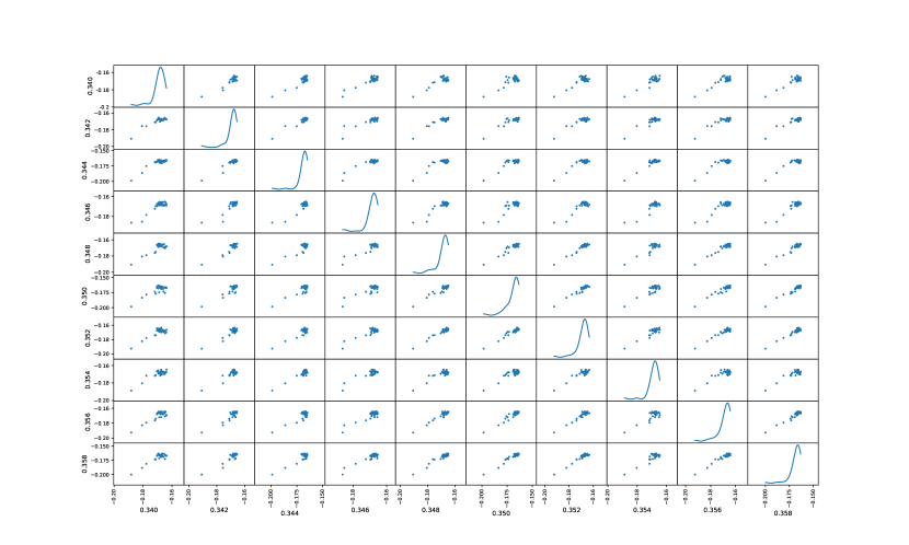
Figure 10: BOSS1 scatter matrix of the bias relation between 10 neighbour bins. Both axes show the average $z$ for each bin.

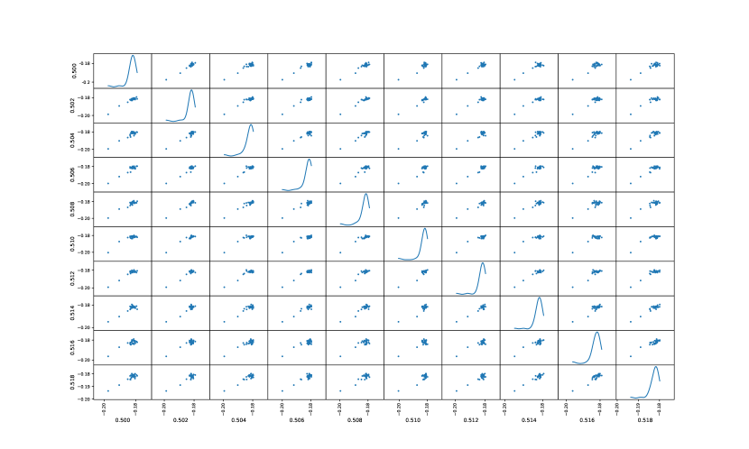
Figure 11: BOSS2 scatter matrix of the bias relation between 10 neighbour bins. Both axes show the average $z$ for each bin.

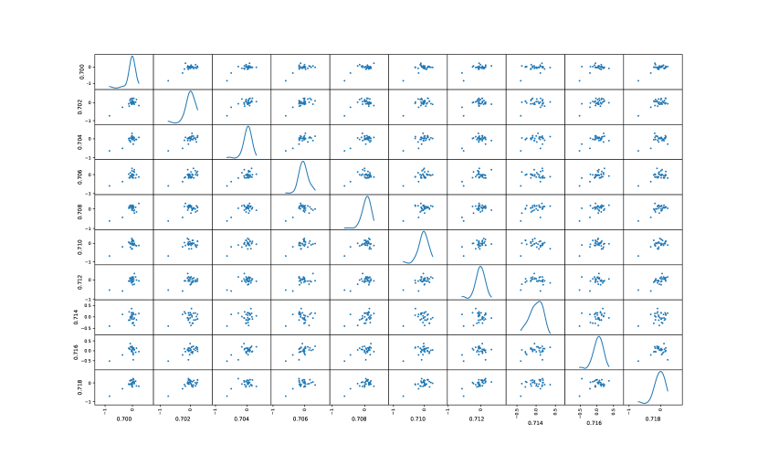
Figure 12: eBOSS scatter matrix of the bias relation between 10 neighbour bins. Both axes show the average $z$ for each bin.

Appendix B BOSS2 triangle plots

In figures 13(a) and 13(b), there are constraints for the separated physical parameters. The $C_{ml}$ results did not perform as well as the real data inference which agrees with the discussion of section 4.2. The mocks should be a good representation, but this is more challenging for a shallower sample. The very different results are a combination of nonlinear effects representation for the mocks and our method not being successful in fixing such issues.

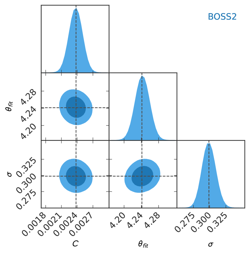
(a) BOSS2 results with $\zeta_{ml}$.

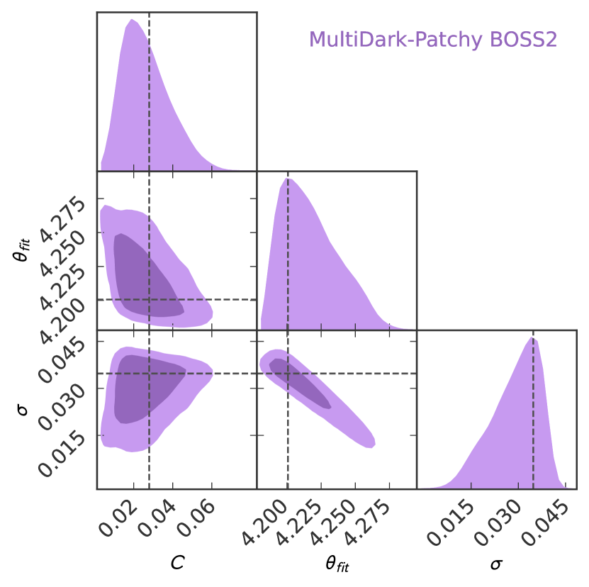
(b) BOSS2 results with $\zeta_{ml}$.

Figure 13: BOSS2 results using pygtc (Bocquet & Carter, 2016).

References

- Aghanim et al. (2020) Aghanim N., et al., 2020, Astronomy & Astrophysics, 641, A6
- Ansari et al. (2019) Ansari R., et al., 2019, Astronomy & Astrophysics, 623, A76
- Anselmi et al. (2016) Anselmi S., Starkman G. D., Sheth R. K., 2016, Monthly Notices of the Royal Astronomical Society, 455, 2474
- Anselmi et al. (2018) Anselmi S., Corasaniti P.-S., Starkman G. D., Sheth R. K., Zehavi I., 2018, Physical Review D, 98, 023527
- Benitez et al. (2014) Benitez N., et al., 2014, arXiv preprint arXiv:1403.5237
- Beutler et al. (2011) Beutler F., et al., 2011, Monthly Notices of the Royal Astronomical Society, 416, 3017
- Bocquet & Carter (2016) Bocquet S., Carter F. W., 2016, Journal of Open Source Software, 1, 46
- Brout et al. (2022) Brout D., et al., 2022, The Astrophysical Journal, 938, 110
- Carvalho et al. (2016) Carvalho G., Bernui A., Benetti M., Carvalho J., Alcaniz J., 2016, Physical Review D, 93, 023530
- Chuang et al. (2015) Chuang C.-H., Kitaura F.-S., Prada F., Zhao C., Yepes G., 2015, Monthly Notices of the Royal Astronomical Society, 446, 2621
- De Mattia et al. (2021) De Mattia A., et al., 2021, Monthly Notices of the Royal Astronomical Society, 501, 5616
- Des Bourboux et al. (2020) Des Bourboux H. D. M., et al., 2020, The Astrophysical Journal, 901, 153
- Eisenstein et al. (2005) Eisenstein D. J., et al., 2005, The Astrophysical Journal, 633, 560
- Feldman et al. (1993) Feldman H. A., Kaiser N., Peacock J. A., 1993, arXiv preprint astro-ph/9304022
- Flaugher & Bebek (2014) Flaugher B., Bebek C., 2014, in Ground-based and Airborne Instrumentation for Astronomy V. pp 282–289
- Foreman-Mackey et al. (2013) Foreman-Mackey D., Hogg D. W., Lang D., Goodman J., 2013, PASP, 125, 306
- Gil-Marín et al. (2020) Gil-Marín H., et al., 2020, Monthly Notices of the Royal Astronomical Society, 498, 2492
- Hand et al. (2018) Hand N., Feng Y., Beutler F., Li Y., Modi C., Seljak U., Slepian Z., 2018, The Astronomical Journal, 156, 160
- Hou et al. (2021) Hou J., et al., 2021, Monthly Notices of the Royal Astronomical Society, 500, 1201
- Kitaura et al. (2016) Kitaura F.-S., et al., 2016, Monthly Notices of the Royal Astronomical Society, 456, 4156
- Klypin & Prada (2018) Klypin A., Prada F., 2018, Monthly Notices of the Royal Astronomical Society, 478, 4602
- Landy & Szalay (1993) Landy S. D., Szalay A. S., 1993, The Astrophysical Journal, 412, 64
- Marra & Chirinos Isidro (2019) Marra V., Chirinos Isidro E. G., 2019, Monthly Notices of the Royal Astronomical Society, 487, 3419
- Menote & Marra (2022) Menote R., Marra V., 2022, Monthly Notices of the Royal Astronomical Society, 513, 1600
- Moster et al. (2011) Moster B. P., Somerville R. S., Newman J. A., Rix H.-W., 2011, The Astrophysical Journal, 731, 113
- Nelson et al. (2013) Nelson B., Ford E. B., Payne M. J., 2013, The Astrophysical Journal Supplement Series, 210, 11
- Peebles (2001) Peebles P., 2001, arXiv preprint astro-ph/0103040
- Percival et al. (2001) Percival W. J., et al., 2001, Monthly Notices of the Royal Astronomical Society, 327, 1297
- Ramírez-Pérez et al. (2022) Ramírez-Pérez C., Sanchez J., Alonso D., Font-Ribera A., 2022, Journal of Cosmology and Astroparticle Physics, 2022, 002
- Reid et al. (2016) Reid B., et al., 2016, Monthly Notices of the Royal Astronomical Society, 455, 1553
- Rodríguez-Torres et al. (2016) Rodríguez-Torres S. A., et al., 2016, Monthly Notices of the Royal Astronomical Society, 460, 1173
- Rosell et al. (2022) Rosell A. C., et al., 2022, Monthly Notices of the Royal Astronomical Society, 509, 778
- Ross et al. (2007) Ross N. P., et al., 2007, Monthly Notices of the Royal Astronomical Society, 381, 573
- Ross et al. (2020) Ross A. J., et al., 2020, Monthly Notices of the Royal Astronomical Society, 498, 2354
- Sánchez et al. (2011) Sánchez E., et al., 2011, Monthly Notices of the Royal Astronomical Society, 411, 277
- Sánchez et al. (2013) Sánchez E., Alonso D., Sánchez F., García-Bellido J., Sevilla I., 2013, Monthly Notices of the Royal Astronomical Society, 434, 2008
- Scaramella et al. (2022) Scaramella R., et al., 2022, Astronomy & Astrophysics, 662, A112
- Scranton et al. (2002) Scranton R., et al., 2002, The Astrophysical Journal, 579, 48
- Seo et al. (2008) Seo H.-J., Siegel E. R., Eisenstein D. J., White M., 2008, The Astrophysical Journal, 686, 13
- Sinha & Garrison (2020) Sinha M., Garrison L. H., 2020, MNRAS, 491, 3022
- Taskesen (2020) Taskesen E., 2020, Distfit, https://erdogant.github.io/distfit
- Wang et al. (2020) Wang Y., et al., 2020, Monthly Notices of the Royal Astronomical Society, 498, 3470
- Xavier et al. (2016) Xavier H. S., Abdalla F. B., Joachimi B., 2016, Monthly Notices of the Royal Astronomical Society, 459, 3693
- Xu et al. (2012) Xu X., Padmanabhan N., Eisenstein D. J., Mehta K. T., Cuesta A. J., 2012, Monthly Notices of the Royal Astronomical Society, 427, 2146
- Zehavi et al. (2002) Zehavi I., et al., 2002, The Astrophysical Journal, 571, 172
- Zehavi et al. (2004) Zehavi I., et al., 2004, The Astrophysical Journal, 608, 16
- Zel’Dovich (1970) Zel’Dovich Y. B., 1970, Astronomy and astrophysics, 5, 84
- Zhao et al. (2021) Zhao C., et al., 2021, Monthly Notices of the Royal Astronomical Society, 503, 1149
- Zhou et al. (2023) Zhou R., et al., 2023, The Astronomical Journal, 165, 58