Optimal Entry and Exit with Signature in Statistical Arbitrage

Abstract

In this paper, we explore an optimal timing strategy for the trading of price spreads exhibiting mean-reverting characteristics. A sequential optimal stopping problem is formulated to analyze the optimal timings for both entering and subsequently liquidating positions, all while considering the impact of transaction costs. Our approach leverages the signature optimal stopping method to resolve this sequential optimal stopping problem, thereby unveiling the precise entry and exit timings that maximize gains. Our framework accommodates a wide range of mean reversion dynamics, offering adaptability to diverse scenarios. Numerical results are provided to demonstrate its superior performance when comparing with conventional mean reversion trading rules.

Keywords— mean-reversion trading; signature method; optimal stopping Time

1 Introduction

Statistical arbitrage, also referred to mean reversion trading, is a trading strategy that employs statistical methods to identify pricing discrepancies between assets and capitalize on them for profit. It is widely used by traders and fund managers to simultaneously establish positions in two correlated assets and speculate on the resultant spread’s path behavior. While modeling the dynamics of a single asset can be challenging, statistical models excel in capturing the mean-reverting behavior exhibited by pairs of assets or securities. The mean reversion trading process comprises three fundamental steps: (1) the identification of co-moving assets, (2) the construction of spreads, and (3) the design of trading rules. The first two steps can be referred to as the formation period, while the last constitutes the trading period.

The process of identifying assets for statistical arbitrage relies on principles grounded in market dynamics, such as the co-movement of risk-on assets in the same direction or the correlation between stocks within a shared sector. For a trading pair to be considered profitable, it is imperative that the two assets exhibit a certain degree of correlation. This strategy entails the simultaneous purchase of one asset and sale of another, thereby achieving market neutrality within the designated group or sector, with the ultimate goal of capitalizing on the subsequent price convergence between these two assets. Empirical research has substantiated the presence of mean-reverting price behavior in various instances, including pairs of stocks and/or ETFs, disparities between futures and their corresponding spot prices, and spreads between physical commodities and commodity stocks/ETFs. Additionally, automated methodologies have been developed to identify portfolios with mean-reverting characteristics. In the context of this paper, we undertake a preliminary selection of several stock pairs in the US market, guided by human expertise, spanning diverse sectors, ranging from airlines to the technology industry. Each pair comprises two stocks originating from the same industry, thereby affording a comprehensive examination of mean reversion within different sectors.

The constructed spreads are essential to possess a mean-reverting characteristic, as this property underpins the opportunities available to traders engaged in statistical arbitrage. To illustrate, when the price of a spread deviates below its long-term mean, traders adopt a long position in the spread and await its reversion to the mean, thereby securing a profitable outcome. In the numerical experiments of the paper, we embrace a statistical approach to construct these spreads. For any given pair of stocks, we configure the spread to best conform to the Ornstein-Uhlenbeck (OU) model. More precisely, we ascertain the optimal ratio between the two stocks, as well as the model parameters, in a manner that maximizes the likelihood of the resulting spread time series. Notably, this method represents an extension of the conventional maximum likelihood estimation (MLE) approach, which traditionally focuses solely on determining the model parameters.

Within the trading period, investors confront the intricate task of deciding the optimal trading rules for both entering and exiting a position, a determination contingent upon the dynamic fluctuations in the price of the risky asset. Investors are presented with the choice of either entering the market immediately or exercising patience while monitoring the prevailing market prices, awaiting a more propitious moment. After executing the initial trade, the investor encounters the consequential decision of pinpointing the most advantageous instance for closing the position. This challenge motivates the central inquiry of our research—namely, the investigation of the optimal timing of trades.

In response to this challenge, we introduce a optimal trading timing framework designed to systematically assess the optimal moments for both initiating and subsequently liquidating positions. Our methodology formulates a sequential optimal stopping problem to analyze the optimal trading timings, and capitalizes on the signature optimal stopping method, a powerful tool for solving this sequential optimal stopping problem, consequently revealing the precise timings for entry and exit that yield maximal gains. Importantly, our framework is adapted to a broad spectrum of mean reversion dynamics, with the Ornstein-Uhlenbeck (OU) model serving as a prime illustration in our experimental investigations.

The remainder of this paper is structured as follows. In Section 2, we offer a comprehensive review of relevant literature. Section 3 lays the foundation by introducing the fundamental concepts pertaining to the signature. Within Section 4, we expound upon the signature optimal stopping method. In Section 5, we elaborate on our proposed framework for optimizing entry and exit decisions, presenting the associated solutions. The empirical validation of our methodology through numerical experiments, encompassing both simulated and real-world data, is detailed in Section 6. Finally, Section 7 provides concluding remarks.

2 Related Research

Examples of mean-reverting spreads are well-documented in a variety of empirical studies spanning diverse asset classes. They have been observed in pairs of stocks and ETFs (Gatev et al. (2006), Avellaneda and Lee (2010), Montana and Triantafyllopoulos (2011), Leung and Li (2016)), futures contracts (Brennan and Schwartz (1990), Dai et al. (2011)), physical commodity and commodity stocks/ETFs (Kanamura et al. (2010)), as well as cryptocurrencies (Leung and Nguyen (2019)).

The work of Gatev et al. (2006) stands as one of the pioneering studies in the realm of mean reversion trading, often referred to as pairs trading due to their method’s reliance on pairs to construct a mean-reverting process. They introduce the widely adopted Distance Method (DM) and conduct empirical testing using CRSP stocks spanning from 1962 to 2002. The DM method initiates a trading position for a pair of assets when their prices deviate from each other by more than two historical standard deviations, subsequently closing the position when the prices converge again. Their findings reveal an excess return of 1.3 $\%$ for the top 5 pairs identified by the DM method and 1.4$\%$ for the top 20 pairs. Furthermore, Do and Faff (2012) delve into the profitability of pairs trading while accounting for transaction costs. Their research extends the understanding of the practicality of pairs trading by incorporating the impact of transaction expenses, offering valuable insights into the real-world feasibility of this trading strategy.

In addition to the Distance Method (DM), cointegration tests are commonly employed in various alternative methods for mean reversion trading. Vidyamurthy (2004) elucidate a cointegration framework for mean reversion trading, drawing inspiration from Engle and Granger’s error correction model representation of cointegrated series as presented in the seminal work of Engle and Granger (1987). Galenko et al. (2012) explore an active ETF trading strategy built upon cointegrated time series. Their research leverages the concept of cointegration to develop trading strategies within the context of exchange-traded funds. Leung and Nguyen (2019) construct cointegrated portfolios of cryptocurrencies using the Engle-Granger two-step approach and the Johansen cointegration test, exemplifying the versatility of cointegration in portfolio construction across diverse asset classes. Huck and Afawubo (2015) undertake a comparative analysis of the performance of the DM method and cointegration-based approaches using the components of the S$\&$P 500 index. This study sheds light on the relative merits of these two methodologies in the context of mean reversion trading.

Another popular approach in mean reversion trading is the stochastic spread method, which characterizes the path behavior of the spread using a stochastic process exhibiting mean-reverting properties. In this methodology, the construction of spreads and the extraction of trading signals typically rely on the analysis of parameters within the underlying stochastic model. For instance, Elliott et al. (2005) introduce a mean-reverting Gaussian Markov chain model to describe the dynamics of spreads. They utilize this model’s estimates in comparison with observed spread data to make informed trading decisions. Expanding on this framework, Do et al. (2006) delve deeper into the methodology proposed by Elliott et al. and present a generalized stochastic residual spread method. This method is designed to model relative mispricing, offering a broader perspective on the stochastic spread approach in mean reversion trading. In their comprehensive work, Leung and Li (2016) provide insights into optimal mean reversion trading strategies founded on various stochastic modeling approaches. Their research encompasses a range of models, including the Ornstein-Uhlenbeck (OU) model, Exponential OU Model, and CIR Model, elucidating how these different models can be leveraged to optimize mean reversion trading strategies. This work contributes to the broader understanding of mean reversion trading by exploring the effectiveness of diverse stochastic frameworks.

Furthermore, various alternative methods for mean reversion trading have emerged in recent years. Some of these methods leverage copulas (Liew and Wu (2013), Xie et al. (2016)), Principal Component Analysis (PCA) (Avellaneda and Lee (2010), and machine learning techniques (Guijarro-Ordonez et al. (2021)) to identify trading opportunities based on statistical patterns and relationships among assets. In addition to these methodologies, new optimization algorithms have been proposed to construct spreads with maximum in-sample mean reversion. Notably, some of these algorithms are designed for automation, enabling the simultaneous analysis of a large number of stocks (d’Aspremont (2011), Leung et al. (2020)). These advancements reflect the ongoing innovation in the field of mean reversion trading, offering traders and researchers a diverse set of tools and techniques to explore.

In the domain of optimal timing strategies for trading mean-reverting spreads, several notable studies have contributed to the understanding of this field. Ekström et al. (2011) investigate the optimal single liquidation timing in the context of the Ornstein-Uhlenbeck (OU) model with zero long-run mean and no transaction costs. Song et al. (2009) introduce a numerical stochastic approximation scheme to solve for optimal buy-low-sell-high strategies over a finite time horizon. Leung and Li (2015) address an optimal double stopping problem, providing optimal entry and exit decision rules. They derive analytical solutions for both the entry and exit problems under the assumption of an OU process. These studies collectively contribute to the advancement of optimal timing strategies for trading mean-reverting spreads, offering various perspectives and methodologies for tackling this challenging problem. The current paper is motivated by the model introduced by these prior researchers, proposing a sequential optimal stopping problem to determine optimal trading times without assuming specific dynamics for the spread.

The utilization of the signature method in the paper to address the optimal stopping problem aligns with recent developments in mathematical finance. Bayer et al. (2021) have introduced a novel approach to solving optimal stopping problems based on signature theory. Importantly, this method does not require specific assumptions about the underlying stochastic process other than it being a continuous (geometric) random rough path. The core concept revolves around considering classic stopping times approximated as signature optimal stopping times, which can be decided through a functional of the signature associated with the stochastic process. Bayer et al. demonstrate that optimizing over these classes of signature stopping times effectively solves the original optimal stopping problem. This transformation allows for the problem to be reformulated as an optimization task dependent solely on the truncated signature. Furthermore, Bayer et al. introduce a numerical solution to the signature optimal stopping problem by formulating the problem as an optimization task involving the minimization of a loss function associated with the truncated signature. This numerical approach provides a practical tool to implement the signature-based framework for solving optimal stopping problems, making it applicable to a wide range of real-world scenarios. They illustrate the practicality of this method in the context of optimal stopping for fractional Brownian motions.

Indeed, motivated by the innovative methodology introduced by Bayer et al. (2021), our paper embarks on an exploration of the potential application of the signature framework to tackle the optimal entry and exit problem in mean reversion trading. This extension highlights the remarkable versatility and promising capabilities of signature-based methods in effectively addressing a wide spectrum of challenges within financial contexts.

3 Preliminaries of Signature

Signature methods play an important role in this paper. In this section, we will introduce the theory of signatures that will serve as a foundational framework for the article.

3.1 Tensor algebra

A signature is an infinite series that takes values in a specific graded space known as the tensor algebra. To provide a solid foundation for understanding signatures, we will begin by introducing the fundamentals of tensor algebra.

The tensor product of two vectors $\mathbf{u}=(u_{i})$ and $\mathbf{v}=(v_{j})$ is given by:

$$(\mathbf{u}\otimes\mathbf{v})_{i,j}=u_{i}v_{j}$$

For example, if $\mathbf{u}=(u_{1},u_{2})\in\mathbb{R}^{2}$ and $\mathbf{v}=(v_{1},v_{2},v_{3})\in\mathbb{R}^{3}$, then their tensor product is given by

$$\mathbf{u}\otimes\mathbf{v}=\begin{pmatrix}u_{1}v_{1}&u_{1}v_{2}&u_{1}v_{3}\\ u_{2}v_{1}&u_{2}v_{2}&u_{2}v_{3}\\ \end{pmatrix}\in\mathbb{R}^{2\times 3}.$$

The concept of the tensor product can indeed be extended to accommodate multiple vectors or tensors. To illustrate, consider the example of taking the 3-way tensor product of three vectors $\mathbf{u}=[1,2],\ \mathbf{v}=[3,4],\ \mathbf{w}=[5,6]$:

$$\begin{pmatrix}1\\ 2\end{pmatrix}\otimes\begin{pmatrix}3\\ 4\end{pmatrix}\otimes\begin{pmatrix}5\\ 6\end{pmatrix}=\begin{pmatrix}1\cdot\begin{pmatrix}3\\ 4\end{pmatrix}\otimes\begin{pmatrix}5\\ 6\end{pmatrix}\\ 2\cdot\begin{pmatrix}3\\ 4\end{pmatrix}\otimes\begin{pmatrix}5\\ 6\end{pmatrix}\end{pmatrix}=\begin{bmatrix}\begin{array}[]{cc}15\ 18\\ 20\ 24\\ \hline\cr 30\ 36\\ 40\ 48\end{array}\end{bmatrix}$$

In this context, the resulting tensor $\mathbf{u}\otimes\mathbf{v}\otimes\mathbf{w}$ is a $2\times 2\times 2$ array, where the $(i,j,k)$-th entry is the product of the $i$-th entry of $u$, the $j$-th entry of $v$, and the $k$-th entry of $w$.

Let $U$ and $V$ represent two vector spaces with bases $\{\mathbf{u}_{1},\ldots,\mathbf{u}_{m}\}$ and $\{\mathbf{v}_{1},\ldots,\mathbf{v}_{n}\}$, respectively. The tensor product space $U\otimes V$ is defined as the vector space formed by the linear combinations of all possible products $\mathbf{u}_{i}\otimes\mathbf{v}_{j}$, where $i$ ranges from 1 to $m$ and $j$ ranges from 1 to $n$. Formally, we express this as follows:

$$U\otimes V=span\{\mathbf{u}_{i}\otimes\mathbf{v}_{j}|1\leq i\leq m,1\leq j\leq n\}.$$

The tensor product space $U\otimes V$ possesses a natural basis $\{\mathbf{u}_{i}\otimes\mathbf{v}_{j}\,|\,1\leq i\leq m,1\leq j\leq n\}$. As an illustrative example, consider $U=\mathbb{R}^{2}$ and $V=\mathbb{R}^{3}$. In this case, the tensor product space $U\otimes V$ has a dimension of $2\times 3=6$, and a possible basis can be represented as follows:

$$\mathbf{u}_{1}\otimes\mathbf{v}_{1} =\begin{pmatrix}1\\ 0\end{pmatrix}\otimes\begin{pmatrix}1\\ 0\\ 0\end{pmatrix}=\begin{pmatrix}1\ 0\\ 0\ 0\\ 0\ 0\\ \end{pmatrix}$$

$$\mathbf{u}_{1}\otimes\mathbf{v}_{2} =\begin{pmatrix}1\\ 0\end{pmatrix}\otimes\begin{pmatrix}0\\ 1\\ 0\end{pmatrix}=\begin{pmatrix}0\ 0\\ 1\ 0\\ 0\ 0\\ \end{pmatrix}$$

$$\vdots$$

$$\mathbf{u}_{2}\otimes\mathbf{v}_{3} =\begin{pmatrix}0\\ 1\end{pmatrix}\otimes\begin{pmatrix}0\\ 0\\ 1\end{pmatrix}=\begin{pmatrix}0\ 0\\ 0\ 0\\ 0\ 1\\ \end{pmatrix}$$

The concept of tensor product for two spaces can be readily extended to multiple spaces. Let $\mathbb{R}^{d}$, where $d\geq 1$, be a finite-dimensional real vector space with a basis $\{\mathbf{e}_{1},\cdots,\mathbf{e}_{d}\}$. Then, $(\mathbb{R}^{d})^{\otimes n}$ is the tensor product of $n$ copies of $\mathbb{R}^{d}$, resulting in a vector space with $d^{n}$ dimensions. Each element in this tensor product space is represented as a tensor formed by taking the tensor product of $n$ vectors, each belonging to $\mathbb{R}^{d}$. We can define a basis for $(\mathbb{R}^{d})^{\otimes n}$ as follows:

$$\{\mathbf{e}_{i_{1}}\otimes\cdots\otimes\mathbf{e}_{i_{n}}\ |\ i_{j}\in\{1,\cdots,d\}\ \text{for}\ j=1,\cdots,n\}.$$

Based on $(\mathbb{R}^{d})^{\otimes n}$, we can provide the definition for the extended tensor algebra.

Definition 3.1

(Extended tensor algebra) The extended tensor algebra over $\mathbb{R}^{d}$ is defined by

$$T((\mathbb{R}^{d})):=\{\textbf{a}=(a_{n})_{n=0}^{\infty}\ |\ a_{n}\in(\mathbb{R}^{d})^{\otimes n}\}.$$

Given $\textbf{a}=(a_{i})_{i=0}^{\infty}$, $\textbf{b}=(b_{i})_{i=0}^{\infty}\in T((\mathbb{R}^{d}))$, define the sum and product by

$$\textbf{a}+\textbf{b}:=(a_{i}+b_{i})_{i=0}^{\infty}$$

$$\textbf{a}\otimes\textbf{b}:=\left(\sum_{k=0}^{i}a_{k}\otimes b_{i-k}\right)_{i=0}^{\infty}.$$

We also define the action on $\mathbb{R}$ given by $\lambda\textbf{a}:=(\lambda a_{i})_{i=0}^{\infty}$ for $\lambda\in\mathbb{R}$.

Likewise, we can define the tensor algebra as the space of all finite sequences of tensors. Additionally, we can define the truncated tensor algebra as the space of sequences of tensors of a specified, fixed length. These definitions allow us to work with sequences of tensors, accommodating various mathematical operations and analyses in this paper.

Definition 3.2

(Tensor algebra) The tensor algebra over $\mathbb{R}^{d}$, denoted by $T(\mathbb{R}^{d})\subset T((\mathbb{R}^{d}))$, is given by

$$T(\mathbb{R}^{d}):=\{\textbf{a}=(a_{n})_{n=0}^{\infty}\ |\ a_{n}\in(\mathbb{R}^{d})^{\otimes n}\ \text{and}\ \exists N\in\mathbb{N}\ \text{such that}\ a_{n}=0\ \forall n\geq N\}.$$

Definition 3.3

(Truncated tensor algebra) The truncated tensor algebra of order $n\in\mathbb{N}$ over $\mathbb{R}^{d}$ is defined by

$$T^{(N)}(\mathbb{R}^{d}):=\{\textbf{a}=(a_{n})_{n=0}^{\infty}\ |\ a_{n}\in(\mathbb{R}^{d})^{\otimes n}\ \text{and}\ a_{n}=0\ \forall n\geq N\}.$$

In the context of the dual space and linear functions on the tensor algebra, let $\{\mathbf{e}_{1}^{*},\cdots,\mathbf{e}^{*}_{d}\}$ be a dual basis for $(\mathbb{R}^{d})^{*}$, where $(\mathbb{R}^{d})^{*}$ represents the dual space of $\mathbb{R}^{d}$. This dual space consists of all continuous linear functions mapping from $\mathbb{R}^{d}$ to $\mathbb{R}$. We can define a basis for $((\mathbb{R}^{d})^{*})^{\otimes n}$ as follows:

$$\{\mathbf{e}^{*}_{i_{1}}\otimes\cdots\otimes\mathbf{e}^{*}_{i_{n}}\ |\ i_{j}\in\{1,\cdots,d\}\ \text{for}\ j=1,\cdots,n\}.$$

We denote the dual space of $T((\mathbb{R}^{d}))$ as $T((\mathbb{R}^{d})^{*}):=((\mathbb{R}^{d})^{*})^{\otimes n}$.

It’s important to note that there exists a natural pairing between $T((\mathbb{R}^{d})^{*})$ and $T((\mathbb{R}^{d}))$, which we denote as $\langle\cdot,\cdot\rangle:T((\mathbb{R}^{d})^{*})\times T((\mathbb{R}^{d}))\rightarrow\mathbb{R}$. Consequently, the dual space $T((\mathbb{R}^{d})^{*})$ encompasses all continuous linear functions defined on the extended tensor algebra $T((\mathbb{R}^{d}))$.

3.2 Signature

We will now introduce a pivotal concept in this paper: the signature of a path. For a given path $X:[0,T]\mapsto\mathbb{R}^{d}$, we denote the coordinate paths as $(X^{1}_{t},\cdots,X^{d}_{t})$, where each $X^{i}:[0,T]\mapsto\mathbb{R}$ represents a real-valued path. For any single index $i\in\{1,\cdots,d\}$ and $0\leq a\leq b\leq T$, we define the quantity:

$$S(X)^{i}_{a,b}=\int_{a<s<b}dX_{s}^{i}=X_{b}^{i}-X_{a}^{i},$$

which signifies the increment of the $i$-th coordinate of the path within the time interval $t\in[a,b]$.

For any pair of indices $i,j\in\{1,\cdots,d\}$, we define the second-order path integral:

$$S(X)^{i,j}_{a,b}=\int_{a<r<s<b}dX_{r}^{i}dX_{s}^{j},$$

and this concept can be generalized to arbitrary orders. For any integer $n\geq 1$ and a collection of indices $i_{1},\cdots,i_{n}\in\{1,\cdots,d\}$, we define:

$$S(X)^{i_{1},\cdots,i_{n}}_{a,b}=\int_{a<t_{1}<\cdots<t_{n}<b}dX_{t_{1}}^{i_{1}}\cdots dX_{t_{n}}^{i_{n}},$$

referred to as the $n$-fold iterated integral of $X$ along the indices $i_{1},\cdots,i_{n}$. The vector comprising all the $n$-fold iterated integrals of $X$ is defined as:

$$\mathbb{X}_{a,b}^{n}:=\left(S(X)^{i_{1},\cdots,i_{n}}_{a,b}\ \vline\ i_{1},\cdots,i_{n}\in\{1,\cdots,d\}\right).$$

In fact, $\mathbb{X}_{a,b}^{n}$ belongs to $(\mathbb{R}^{d})^{\otimes n}$, and we can express it concisely using the tensor product symbol:

$$\mathbb{X}_{a,b}^{n}=\int_{a<t_{1}<\cdots<t_{n}<b}dX_{t_{1}}\otimes\cdots\otimes dX_{t_{n}}\in(\mathbb{R}^{d})^{\otimes n}.$$

Example 3.4

Consider a path $X:[0,T]\mapsto\mathbb{R}^{3}$, then

$$\mathbb{X}_{a,b}^{1}=\left(S(X)^{1}_{a,b},S(X)^{2}_{a,b},S(X)^{3}_{a,b}\right),$$

$$\mathbb{X}_{a,b}^{2}=\left(S(X)^{1,1}_{a,b},S(X)^{1,2}_{a,b},S(X)^{1,3}_{a,b},S(X)^{2,1}_{a,b},S(X)^{2,2}_{a,b},S(X)^{2,3}_{a,b},S(X)^{3,1}_{a,b},S(X)^{3,2}_{a,b},S(X)^{3,3}_{a,b}\right).$$

Now, we can introduce the definition of a signature.

Definition 3.5

(Signature) Let $0\leq a<b\leq T$. For a path $X:[0,T]\rightarrow\mathbb{R}^{d}$, we define the signature of $X$ over $[a,b]$ by

$$\mathbb{X}_{a,b}^{<\infty}:=(1,\mathbb{X}_{a,b}^{1},\cdots,\mathbb{X}_{a,b}^{n},\cdots)\in T((\mathbb{R}^{d})),$$

where

$$\mathbb{X}_{a,b}^{n}:=\int_{a<t_{1}<\cdots<t_{n}<b}dX_{t_{1}}\otimes\cdots\otimes dX_{t_{n}}\in(\mathbb{R}^{d})^{\otimes n}.$$

Similarly, the truncated signature of order $N$ is defined by

$$\mathbb{X}_{a,b}^{\leq N}:=(1,\mathbb{X}_{a,b}^{1},\cdots,\mathbb{X}_{a,b}^{N})\in T^{(N)}((\mathbb{R}^{d})).$$

If we refer to the signature of $X$ without specifying the interval over which the signature is taken, we will implicitly refer to $\mathbb{X}_{0,T}^{<\infty}$.

In practical applications of the signature method, we typically transform the original path into an augmented path and then compute the truncated signature of the augmented path as the input features for any algorithm.

Given a $d$-dimensional path $X_{t}:[0,T]\rightarrow\mathbb{R}^{d}$, we denote its augmentation by $\widehat{X}_{t}=(t,X_{t})\in\mathbb{R}^{1+d}$, and define $\widehat{\mathbb{X}}^{\leq\infty}$ and $\widehat{\mathbb{X}}^{\leq\lfloor p\rfloor}$ as the signature and $\lfloor p\rfloor$-truncated signature of $\widehat{X}_{t}$, respectively. Then, we define the space $\widehat{\Omega}^{p}_{T}$ as the closure of all the $p$-truncated signatures. In other words, elements of $\widehat{\Omega}^{p}_{T}$ are $p$-truncated signatures of some augmented paths $(t,X_{t})$. Due to the first dimension of the augmented path being monotonically increasing, the signature $\widehat{\mathbb{X}}^{\leq\infty}$ provides a complete characterization of $\widehat{X}$ (and therefore $X$). See Hambly and Lyons(2010). However, computing the entire signature with infinite length is not feasible, so the truncated signature with a fixed order $p$ is used in the practice of the signature method. As a result, the time series to be analyzed in this paper will first be transformed into the space of $\widehat{\Omega}^{p}_{T}$ for analysis.

4 Signature Optimal Stopping Method

In this section, we introduce the signature optimal stopping method proposed by Bayer et al.(2021), which will be applied in our approach to solve the proposed sequential optimal stopping problems.

The general optimal stopping problem involves determining an optimal stopping time that maximizes the value of the underlying process. Fix the probability space $(\Omega,\mathcal{F},\mathbb{P})$. Suppose $X_{t}$ is a stochastic process and denote the filtration generated by $X$ as $(\mathcal{F}_{t})$, $\mathcal{F}_{t}=\sigma(X_{s}:0\leq s\leq t)$. Consider a payoff process $Y:[0,T]\times\Omega\rightarrow\mathbb{R}$ being a real-valued continuous stochastic process adapted to the filtration $(\mathcal{F}_{t})$, then the optimal stopping problem for $Y_{t}$ is

$$\sup_{\tau\in\mathcal{T}}\mathbb{E}[Y_{\tau\wedge T}],$$ (1)

where $\tau$ is a stopping time adapted to $(\mathcal{F}_{t})$ and $\mathcal{T}$ is the space of all $(\mathcal{F}_{t})$-stopping times

The definition of signature optimal stopping problem is similar to the general optimal stopping problem above, with the key difference lying in the filtration used. Let $(\Omega,{\mathcal{F}},\mathbb{P})$ be a probability space. Given a $d$-dimensional path $X_{t}:[0,T]\rightarrow\mathbb{R}^{d}$ and $\widehat{\mathbb{X}}$ denotes its augmented signature in $\widehat{\Omega}_{T}^{p}$. The filtration generated by the signatures are defined as $(\mathcal{G}_{t})$, $\mathcal{G}_{t}=\sigma(\widehat{\mathbb{X}}_{0,s}:0\leq s\leq t)$ and denote by $\mathcal{S}$ the space of all $(\mathcal{G}_{t})$-stopping times. $\mathcal{S}$ is referred as the space of signature stopping times. Consider a payoff process $Y:[0,T]\times\Omega\rightarrow\mathbb{R}$ being a real-valued continuous stochastic process adapted to the filtration $(\mathcal{G}_{t})$, then the signature optimal stopping problem for $Y_{t}$ is:

$$\sup_{\tau\in\mathcal{S}}\mathbb{E}[Y_{\tau\wedge T}]$$ (2)

where $\tau$ is a signature stopping time adapted to $(\mathcal{G}_{t})$.

In Section 5, we will formulate a sequence of signature optimal stopping problems to address the optimal timing strategy for trading a mean-reverting price spread. This intricate problem will be solved using the signature optimal stopping method. In the following subsection, we will provide a detailed introduction to the implementation of the signature optimal stopping method.

4.1 Randomized Stopping Time

The fundamental concept for addressing the signature optimal stopping problem lies in the utilization of randomized stopping times. As demonstrated by Bayer et al., randomized stopping times are, in fact, equivalent to signature stopping times. Consequently, the signature optimal stopping problem, as depicted in Equation 2, can be effectively transformed into an equivalent problem known as the randomized optimal stopping problem.

Firstly, we define randomized stopping times associated with continuous stopping policies and demonstrate that general stopping times can be approximated by randomized stopping times based on continuous stopping policies. For a given time horizon $T>0$, we define $\Lambda_{T}:=\bigcup_{t\in[0,T]}\widehat{\Omega}_{t}^{p}$, referring to it as the space of stopped signatures. Specifically, we characterize a continuous stopping policy as a Borel measurable mapping $\theta:\Lambda_{T}\rightarrow\mathbb{R}$, and denote the space of continuous stopping policies as $\Theta:=C(\Lambda_{T},\mathbb{R})$. It’s worth noting that we refer to $\theta$ as a stopping policy because it can be employed to define a stopping time based on its mapping value.

Definition 4.1

(Randomized stopping time) Let $Z$ be a non-negative random variable independent of $\widehat{\mathbb{X}}$ and such that $P(Z=0)=0$. For a continuous stopping policy $\theta\in\Theta$, we define the randomized stopping time by

$$\tau^{r}_{\theta}:=\inf\left\{t\geq 0:\int_{0}^{t\wedge T}\theta(\widehat{\mathbb{X}}|_{[0,s]})^{2}ds\geq Z\right\}$$ (3)

where $\inf\phi=+\infty$.

Randomized stopping times, which are derived from continuous stopping policies, possess the capability to approximate general stopping times, as demonstrated in the following theorem [2, Proposition 4.2].

Theorem 4.2

For every stopping time $\tau\in\mathcal{S}$, there exists a sequence $\theta_{n}\in\Theta$ such that the randomized stopping times $\tau^{r}_{\theta_{n}}$ satisfy $\tau^{r}_{\theta_{n}}\rightarrow\tau$ almost surely as $n\rightarrow\infty$. In particular, if $\mathbb{E}[\|Y\|_{\infty}]<\infty$, then

$$\sup_{\theta\in\Theta}\mathbb{E}[Y_{\tau_{\theta}^{r}\wedge T}]=\sup_{\tau\in\mathcal{S}}\mathbb{E}[Y_{\tau\wedge T}].$$ (4)

An astonishing result is that the general stopping time can be approximated by using stopping policies that are linear functions of the signature. The space of linear signature stopping policies $\Theta_{sig}\subset\Theta$ is defined as

$$\Theta_{sig}=\{\theta\in\Theta:\exists l\in T((\mathbb{R}^{1+d})^{*})\ \text{such that}\ \theta(\widehat{\mathbb{X}}|_{[0,t]})=\langle l,\widehat{\mathbb{X}}_{0,t}^{<\infty}\rangle\ \forall\widehat{\mathbb{X}}|_{[0,t]}\in\Lambda_{T}\}.$$

Note that every $l\in T((\mathbb{R}^{1+d})^{*})$ defines a stopping policy $\theta_{l}\in\Theta$ by setting $\theta(\widehat{\mathbb{X}}|_{[0,t]})=\langle l,\widehat{\mathbb{X}}_{0,t}^{<\infty}\rangle$. Then we introduce the following notation for randomized stopping times associated to linear signature stopping policies

$$\tau^{r}_{l}:=\tau^{r}_{\theta_{l}}=\inf\left\{t\geq 0:\int_{0}^{t\wedge T}\langle l,\widehat{\mathbb{X}}_{0,s}^{<\infty}\rangle^{2}ds\geq Z\right\}.$$ (5)

The subsequent theorem, detailed in [2, Proposition 5.3], demonstrates that the randomized stopping times linked to linear signature stopping policies are able to approximate general randomized stopping times.

Theorem 4.3

Assume that $Z$ has a continuous density and $\mathbb{E}[\|Y\|_{\infty}]<\infty$. Then

$$\sup_{\theta\in\Theta}\mathbb{E}[Y_{\tau_{\theta}^{r}\wedge T}]=\sup_{\theta\in\Theta_{sig}}\mathbb{E}[Y_{\tau_{\theta}^{r}\wedge T}].$$

It follows that

$$\sup_{\theta\in\Theta}\mathbb{E}[Y_{\tau_{\theta}^{r}\wedge T}]=\sup_{l\in T((\mathbb{R}^{1+d})^{*})}\mathbb{E}[Y_{\tau_{l}^{r}\wedge T}].$$ (6)

Continuing our exploration, we turn our attention to the evaluation of the optimal stopping problem with regard to a specific stopping policy $\theta$. This evaluation plays a crucial role as it serves as a pivotal loss function, which will be utilized in the process of identifying the optimal linear policy during training. [2, Proposition 4.4] offers comprehensive details into this matter.

Theorem 4.4

Let $F_{Z}$ denote the cumulative distribution function of $Z$. Then

$$\mathbb{E}[Y_{\tau^{r}_{\theta}\wedge T}]=\int_{0}^{T}Y_{t}d\widetilde{F}(t)+Y_{T}(1-\widetilde{F}(T))=\int_{0}^{T}(1-\widetilde{F}(t))dY_{t}+Y_{0}$$ (7)

where the second integral is implicitly defined by integration by parts and

$$\widetilde{F}(t):=F_{Z}\left(\int_{0}^{t}\theta(\widehat{\mathbb{X}}|_{[0,s]})^{2}ds\right).$$

In particular, if $Z$ has a density $f_{Z}$,

$$\mathbb{E}[Y_{\tau^{r}_{\theta}\wedge T}]=\int_{0}^{T}Y_{t}\ \theta(\widehat{\mathbb{X}}|_{[0,t]})^{2}\ f_{Z}\left(\int_{0}^{t}\theta(\widehat{\mathbb{X}}|_{[0,s]})^{2}ds\right)dt+Y_{T}(1-\widetilde{F}(T)).$$

The use of stopping times derived from signature stopping policies for approximation doesn’t inherently demand randomization. In fact, if we substitute the random variable $Z$ in Equation (3) and (5) with any positive constant $k>0$, Equations (4) and (6) will remain applicable. The computation of the optimal stopping value as shown in Equation (7) remains valid as well, and the cumulative distribution function $F_{Z}$ will simplify to a straightforward indicator function. This flexibility in handling randomization underscores the versatility of the signature-based approach in solving complex optimization problems.

In our algorithm, we will utilize stopping times associated with linear signature stopping policies, denoted as $\tau^{r}_{l}$, with respect to a positive constant $k$ to determine the optimal stopping times. This constant $k$ serves as a hyper-parameter, granting us the flexibility to finely adjust the stopping time according to specific timing preferences and requirements. The initial step involves identifying the optimal linear stopping policy, denoted as $l^{*}$, based on the training paths. Subsequently, we can approximate the optimal stopping time by computing the stopping times associated with the optimal linear signature stopping policies $l^{*}$.

4.2 Implementation of signature optimal stopping method

In this section, we will introduce the details of implementing the signature Assume we have a $d$-dimensional process denoted as $X_{t}$, and a continuous real-valued payoff process $Y_{t}$ adapted to the filtration generated by $X_{t}$ for $0\leq t\leq T$.

Our initial step involves discretizing the paths, where we establish a time grid comprising equidistant points denoted as $\{t_{j}\}_{j=0,1,\ldots,n}$, with $t_{j}=\frac{j}{n}T$. To simplify matters, we introduce the discretized path and payoff process as follows: $\widetilde{X}_{j}=X_{t_{j}}$ and $\widetilde{Y}_{j}=Y_{t_{j}}$, where $j=0,1,\ldots,n$. Furthermore, we define the filtration generated by the discretized path as:

$$\widetilde{\mathcal{F}}_{j}:=\sigma(\widetilde{X}_{i}:0\leq i\leq j),\ j=0,1,\ldots,n.$$

We denote $\mathcal{S}_{J}$ as the set of discrete stopping times with respect to this filtration. Consequently, we can approximate the value of the optimal stopping problem with the value of the discrete-time optimal stopping problem:

$$\sup_{\nu\in\mathcal{S}_{J}}\mathbb{E}[\widetilde{Y}_{\nu\wedge n}]=\sup_{\tau\in\mathcal{S}}\mathbb{E}[Y_{\tau\wedge T}].$$

This discretization facilitates the analysis of our problem and enables us to work with discrete-time paths in the practise.

For calculating the signature of discrete paths, we need to define the linear interpolation of the process $X$,

$$\widetilde{X}_{t}=X_{t_{j}}+\frac{t-t_{j}}{t_{j+1}-t_{j}}(X_{t_{j+1}}-X_{t_{j}}),\ t_{j}\leq t\leq t_{j+1},\ j=0,1,\cdots,n-1.$$

Following the discretization step, we proceed by computing the signature of the time-augmented path, denoted as $(t,\widetilde{X}_{t})_{0\leq t\leq T}$, and represent it as $\widetilde{\mathbb{X}}$. Now, we adapt the definition of randomized stopping times to the discrete-time setting. Given a positive random variable $Z$ and a continuous stopping rule $\theta\in\mathcal{T}$, we define the discrete version of the randomized stopping time as follows:

$$\nu^{r}_{\theta}:=\inf\left\{0\leq j\leq n:\sum_{i=0}^{j}\theta(\widetilde{\mathbb{X}}|_{[0,t_{i}]})^{2}\geq Z\right\}$$ (8)

Note that in the context of discrete scenario, we exclusively utilize the values on time grid $\{t_{j}\}_{j=0,1,\ldots,n}$. The discrete version of randomized stopping times associated with linear signature stopping policies is defined as:

$$\nu^{r}_{l}:=\inf\left\{0\leq j\leq n:\sum_{i=0}^{j}\langle l,\widetilde{\mathbb{X}}^{<\infty}_{0,t_{i}}\rangle^{2}\geq Z\right\}$$ (9)

The similar results established in Theorems 4.2 to 4.4 also extend to discrete stopping times. Building upon Theorem 4.4, we can represent the expected payoff as follows:

$$\mathbb{E}[\widetilde{Y}_{\nu^{r}_{\theta}}]=\sum_{j=0}^{n-1}G(j)(\widetilde{Y}_{j+1}-\widetilde{Y}_{j})+\widetilde{Y}_{0},\ \text{where}\ G(j)=1-F_{Z}\left(\sum_{i=0}^{j}\theta(\widetilde{\mathbb{X}}|_{[0,t_{i}]})^{2}\right).$$ (10)

We can further elaborate on the loss function for linear stopping policies based on the regular form of the expected payoff provided above. Given a data-set comprising $M$ samples in the format $(\widetilde{X}_{j}^{(m)},\widetilde{Y}_{j}^{(m)})_{1\leq m\leq M,0\leq j\leq n}$ and a predetermined truncation level $N\geq 1$, we compute the $N$-truncated signature of the linearly interpolated augmented path on each sub-interval $[0,t_{j}]$ for each series of samples. For simplicity, we define

$$\widetilde{\mathbb{X}}_{j}^{(m)}:=\widetilde{\mathbb{X}}_{0,t_{j}}^{(m)},$$

where $1\leq m\leq M$ and $0\leq j\leq n$. Subsequently, we establish the following loss function for the linear stopping policy $\theta_{l}$ based on Equation (12):

$$\text{loss}(l)=-\frac{1}{M}\sum_{i=1}^{M}\left\{\widetilde{Y}_{0}^{(m)}+\sum_{j=0}^{n-1}G_{Z}\left(\sum_{i=0}^{j}\langle l,\widetilde{\mathbb{X}}_{i}^{(m)}\rangle^{2}\right)(\widetilde{Y}^{(m)}_{j+1}-\widetilde{Y}^{(m)}_{j})\right\},$$ (11)

where $G_{Z}=1-F_{Z}$.

In this paper, we’ve opted to replace the random variable $Z$ with a constant $k$ to provide a deterministic solution for the optimal stopping time. Specifically, to compute the optimal stopping time associated with a linear signature stopping policy $l$, the random variable $Z$ in (9) is replaced with a positive constant $k$. The non-randomized stopping time associated with linear signature stopping policies is then defined as follows:

$$\nu_{l}:=\inf\left\{0\leq j\leq n:\sum_{i=0}^{j}\langle l,\widetilde{\mathbb{X}}^{<\infty}_{0,t_{i}}\rangle^{2}\geq k\right\},$$ (12)

where $k$ is a positive constant. This approach allows us to compute the stopping time without relying on randomness, offering a deterministic solution.

Therefore, in our practical implementation, we can employ $\nu_{l}$ to approximate the optimal stopping time. In other words, we calculate the optimal stopping time based on Equation (12) once we have determined the optimal linear stopping policy $l^{*}$.

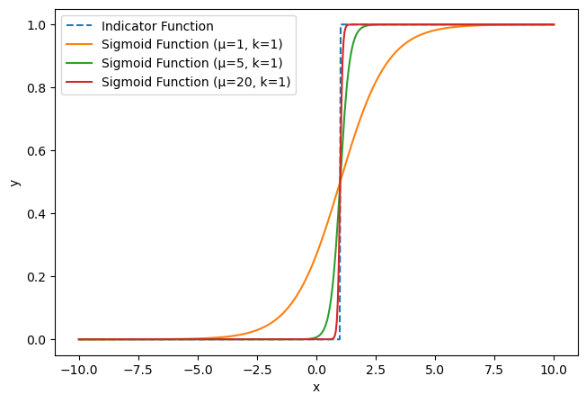
To derive the optimal linear policy, we propose a refinement to the loss function, as originally defined in Equation (11). Initially, we substitute $G_{Z}$ with $G_{k}$, defined as $G_{k}=1-F_{k}$. Here, $F_{k}(x)=\mathbb{I}\{x>k\}$, with $\mathbb{I}$ as the indicator function. To facilitate gradient-based optimization, we approximate $F_{k}$ using a sigmoid function centered at $k$. The approximation $\widehat{F}_{k}(x)$ is given by:

$$\widehat{F}_{k}(x)=\frac{1}{1+e^{-\mu\cdot(x-k)}}$$

where $\mu$ is a large positive constant that sharpens the sigmoid function. Figure 1 illustrates the approximation of the indicator function using a sigmoid function, providing a visual representation of how the sigmoid curve serves as a smoothed substitute for the step-like behavior of the indicator function. In the subsequent experiments, we employ a $\mu$ value of 20.

Figure 1: Approximating indicator function using sigmoid function.

Subsequently, we employ the following modified loss function in our practical implementation:

$$\text{loss}(l)=-\frac{1}{M}\sum_{i=1}^{M}\left\{\widetilde{Y}_{0}^{(m)}+\sum_{j=0}^{n-1}\widehat{G}_{k}\left(\sum_{i=0}^{j}\langle l,\widetilde{\mathbb{X}}_{i}^{(m)}\rangle^{2}\right)(\widetilde{Y}^{(m)}_{j+1}-\widetilde{Y}^{(m)}_{j})\right\},$$ (13)

where $\widehat{G}_{k}=1-\widehat{F}_{k}$. This formulation allows for gradient-based methods to be effectively employed for optimization.

In this section, we have provided a comprehensive overview of our implementation process, with a particular emphasis on the construction of a loss function tailored for linear stopping policies. This loss function serves as a crucial component in our training procedure, facilitating the identification of the optimal linear policy within the signature-based optimal stopping method. Upon successfully obtaining the optimal linear policy, we proceed to compute the corresponding optimal stopping time using Equation (12). This comprehensive methodology underscores our approach to solving complex sequential optimal stopping problems within the signature framework.

5 Signature Optimal Trading

The main contribution of this paper is the development of an innovative trading strategy tailored for mean reversion markets. Our methodology hinges on the formulation of a sequence of optimal stopping problems, aimed at identifying the most advantageous moments for both market entry and exit.

In addition, we propose a solution to these optimal stopping problems through a sequential signature-based optimal stopping framework. This serves as a robust approximation to the broader, more general optimal stopping challenges commonly found in financial mathematics. Notably, our approach is highly adaptable, accommodating any form of mean-reverting dynamics. This framework empowers us to derive a sequence of optimal timing solutions for trading activities, thereby elevating the existing mean-reversion trading rules in both theoretical constructs and real-world applications.

5.1 Long Strategy

Given that a price process or portfolio value following a mean-reverting process, our primary goal is to investigate the optimal timing for opening a long position and subsequently closing the position, while taking into account transaction costs and discount rates. To achieve this, we first introduce a framework that involves solving a sequence of optimal stopping problems.

Suppose that the investor trades on a spread or portfolio whose value process $(X_{t})_{t\geq 0}$ follows a mean reverting process. Recall that $\widehat{\mathbb{X}}$ denotes the augmented signature of $X_{t}$ and the filtration generated by signatures is $(\mathcal{G}_{t})$, where $\mathcal{G}_{t}=\sigma(\widehat{\mathbb{X}}_{0,s}:0\leq s\leq t)$. Denote by $\mathcal{S}$ the space of all $(\mathcal{G}_{t})$-stopping times.

Let us define the shorthand notation for the expectation conditional on the starting value $x$ as $E_{x}\{\cdot\}:=E\{\cdot|X_{0}=x\}$. If the long position is opened at some time $\tau_{0}>0$, then the investor will pay the value $X_{\tau_{0}}$ plus a constant transaction cost $c>0$. Assuming that $r>0$ is the investor’s subjective constant discount rate, the total cost of entering a long position is $e^{-r\tau_{0}}(X_{\tau_{0}}+c)$. Our goal is to minimize the expectation of the entering cost. Therefore, we obtain the following optimal stopping problem for finding the optimal time of entering a long position:

$$\sup_{\tau_{0}\in\mathcal{S}}E_{x_{0}}\{e^{-r\tau_{0}}(-X_{\tau_{0}}-c)\},$$ (14)

where $\mathcal{S}$ is the space of all $(\mathcal{F}_{t})$-stopping times. In a word, we are minimizing the expected cost of entering a long position, given the initial point $x_{0}$.

After obtaining the optimal time to enter a long position, denoted by $\tau_{0}^{*}$, the next question is when to exit the position. If the position is closed at time $\nu_{0}$, the investor will receive the value $X_{\nu_{0}}$ and pay a constant transaction cost $\hat{c}>0$. To maximize the expected discounted value, the investor solves the optimal stopping problem:

$$\sup_{\nu_{0}\in\mathcal{S}}E_{x_{\tau^{*}_{0}}}\{e^{-\hat{r}\nu_{0}}(X_{\nu_{0}}-\hat{c})\}.$$ (15)

Here, we aim to maximize the expectation of discounted earnings conditional on the starting point $x_{\tau^{*}_{0}}$. Note that the pre-entry and post-entry discount rates, $\hat{r}$ and $r$, as well as the entry and exit transaction costs $\hat{c}$ and $c$, can differ in our analysis.

Then we can solve a sequence of optimal stopping problems iteratively to obtain the optimal entry and exit times. That is, for $i=1,2,3,\ldots$, we solve the following equations iteratively:

$$\sup_{\tau_{i}\in\mathcal{S}}E_{x_{\nu_{i-1}^{*}}} \{e^{-r\tau_{i}}(-X_{\tau_{i}}-c)\},$$ (16)

$$\sup_{\nu_{i}\in\mathcal{S}}E_{x_{\tau^{*}_{i}}} \{e^{-\hat{r}\nu_{i}}(X_{\nu_{i}}-\hat{c})\}.$$

Thus, we get the optimal times of trading $\{\tau^{*}_{0},\nu^{*}_{0},\tau^{*}_{1},\nu^{*}_{1},\tau^{*}_{2},\nu^{*}_{2},\cdots\}$.

5.2 Short Strategy

In the short strategy, our main objective is to determine the optimal timing for opening and subsequently closing a short position, similar to the long strategy. We only need to change the order of equations for the optimal stopping problems in (16). Specifically, we obtain the first optimal entry time $\nu_{0}^{*}$ and exit time $\tau_{0}^{*}$ by solving:

$$\sup_{\nu_{0}\in\mathcal{S}}E_{x_{0}}\{e^{-r\nu_{0}}(X_{\nu_{0}}-c)\},$$ (17)

$$\sup_{\tau_{0}\in\mathcal{S}}E_{x_{\nu_{0}^{*}}}\{e^{-\hat{r}\tau_{0}}(-X_{\tau_{0}}-\hat{c})\}.$$

Next, we solve the following equations iteratively for $i=1,2,3,\cdots$:

$$\sup_{\nu_{i}\in\mathcal{S}}E_{x_{\tau_{i-1}^{*}}} \{e^{-r\nu_{i}}(X_{\nu_{i}}-c)\},$$ (18)

$$\sup_{\tau_{i}\in\mathcal{S}}E_{x_{\nu^{*}_{i}}} \{e^{-\hat{r}\tau_{i}}(-X_{\tau_{i}}-\hat{c})\}$$

to obtain the optimal trading times $\{\nu^{*}_{0},\tau^{*}_{0},\nu^{*}_{1},\tau^{*}_{1},\nu^{*}_{2},\tau^{*}_{2},\cdots\}$. The intuition behind is opening a short position when the spread price reaches a high value, and closing the position as the price drops significantly.

5.3 Signature Optimal Stopping Method

The signature optimal stopping method is a powerful technique for solving a sequence of optimal stopping problems. To apply the signature optimal stopping method in our problem, the focus is on generating training samples of the underlying stochastic process and its corresponding payoff process, and then using the signature of the training path as a feature to train an optimal linear stopping policy.

The method can be applied to both long and short strategies, but we will focus on the long strategy in this discussion. In the long strategy, we assume that the underlying process $X_{t}$ follows a one-dimensional Ornstein-Uhlenbeck (OU) process, and that the continuous real-valued payoff process $Y_{t}$ is adapted to the filtration $(\mathcal{F}_{t})$, where $0\leq t\leq T$. The payoff process is given by $Y_{t}=e^{-rt}(-X_{t}-c)$, where $r$ is the risk-free interest rate, $c$ is a constant transaction cost, and $e^{-rt}$ is the discount factor.

To apply the signature optimal stopping method, we first generate training samples of $X_{t}$ starting at a given initial value $x$, and the corresponding $Y_{t}$. We then use these samples to minimize the loss function given in equation (13) to obtain the optimal linear function $l_{1}^{*}$.

Once we obtain the optimal linear stopping policy $l_{1}^{*}$, we can use it to approximate the optimal entry time $\tau^{*}$ by the linear randomized optimal stopping time defined in equation (12). Specifically, the optimal entry time is given by:

$$\tau^{*}=\inf\left\{0\leq j\leq n:\sum_{i=0}^{j}\langle l_{1}^{*},\widehat{\mathbb{X}}_{0,t_{i}}^{\leq N}\rangle^{2}\geq k\right\}$$

where $n$ is the number of discretization intervals, $\widehat{\mathbb{X}}_{0,t_{i}}^{\leq N}$ is the $N$-truncated signature of the path of $(t,X_{t})$ from time $0$ to time $t_{i}$, and $k$ is a positive threshold value.

To solve the optimal exit problem, we need to generate sample paths of $X_{t}$ following an OU process starting from $X_{\tau^{*}}$, and the payoff process $Y_{t}=e^{-\hat{r}t}(X_{t}-\hat{c})$. We then calculate another optimal linear function $l_{2}^{*}$ using the generated samples, and the optimal exit time is given by:

$$\nu^{*}=\inf\left\{0\leq j\leq n:\sum_{i=0}^{j}\langle l_{2}^{*},\widehat{\mathbb{X}}_{\tau^{*},\tau^{*}+t_{i}}^{\leq N}\rangle^{2}\geq k\right\}$$

where $\widehat{\mathbb{X}}_{\tau^{*},\tau^{*}+t_{i}}^{\leq N}$ is the $N$-truncated signature of the path of $X_{t}$ from time $\tau^{*}$ to time $\tau^{*}+t_{i}$. We can continue this computation process to solve the sequence of problems in (16) and thus obtain $\{\tau^{*}_{0},\nu^{*}_{0},\tau^{*}_{1},\nu^{*}_{1},\tau^{*}_{2},\nu^{*}_{2},\cdots\}$, where each pair of values $(\tau^{*}_{n},\nu^{*}_{n})$ corresponds to the optimal entry and exit times for the $n$-th trading.

To be more specific, we use the previously obtained exit time $\nu_{n}^{*}$ as the starting point to solve for the next entry time $\tau_{n+1}^{*}$. We can generate sample paths of $X_{t}$ following an OU process starting from $X_{\nu_{n}^{*}}$ and the payoff $Y_{t}=e^{-rt}(-X_{t}-c)$, and then apply the signature optimal stopping method as before to obtain the optimal linear function $l^{*}_{{n+1},1}$ and entry time $\tau_{n+1}^{*}$.

After obtaining $\tau_{n+1}^{*}$, we can generate sample paths of $X_{t}$ following an OU process starting from $X_{\tau_{n+1}^{*}}$ and the payoff $Y_{t}=e^{-\hat{r}t}(X_{t}-\hat{c})$, where $\hat{r}$ and $\hat{c}$ are the interest rate and constant cost for holding the asset, respectively. Then, we apply the signature optimal stopping method again to obtain the optimal linear function $l^{*}_{{n+1},2}$ and the exit time $\nu_{n+1}^{*}$.

We can then repeat this process to solve for the next entry and exit times until the end of the trading period is reached. Specifically, for $n\geq 0$, we have:

$$\text{Generate sample paths of }X_{t}\text{ starting from }X_{\nu_{n}^{*}}\text{ and }Y_{t}=e^{-rt}(-X_{t}-c)$$

$$\text{Use the signature optimal stopping method to obtain }l^{*}_{{n+1},1}\text{ and }\tau_{n+1}^{*}$$

$$\text{Generate sample paths of }X_{t}\text{ starting from }X_{\tau_{n+1}^{*}}\text{ and }Y_{t}=e^{-\hat{r}t}(X_{t}-\hat{c})$$

$$\text{Use the signature optimal stopping method to obtain }l^{*}_{{n+1},2}\text{ and }\nu_{n+1}^{*}$$

We can continue this process until we reach the end of the trading period. At each step, we obtain the optimal linear function and the corresponding optimal stopping time, which can be used to guide our trading decisions.

In summary, the signature optimal stopping method provides an efficient way to solve a sequence of optimal stopping problems. It requires generating training samples of the underlying stochastic process and its corresponding payoff process, and then using the signature of the path as a feature to approximate the optimal stopping time.

6 Numerical Experiments

In this section, we undertake numerical experiments to rigorously assess the efficacy of our proposed methodologies. We initiate our evaluation by scrutinizing the performance of the proposed optimal trading timing approach through its application to simulated mean reversion spreads. Following this, we extend our analysis to real-world scenarios by evaluating the mean reversion trading performance of our method across four carefully chosen, highly correlated asset pairs in the U.S. stock markets.

6.1 Optimal Stopping for Mean Reversion Process

In this section, we conduct simulations to gauge the effectiveness of our signature-based optimal stopping method in the context of mean reversion spreads. We employ the Ornstein-Uhlenbeck (OU) process to simulate a mean-reverting spread, governed by the following stochastic differential equation:

$$dX_{t}=\theta(\mu-X_{t})dt+\sigma dW_{t}.$$

Our primary aim is to identify the supremum of the expected value of the OU process at the optimal stopping time, formally expressed as:

$$\sup_{\tau\in\mathcal{T}}\mathbb{E}[X_{\tau\wedge T}].$$

By leveraging this simulation framework, we intend to rigorously evaluate the capability of the signature optimal stopping method to accurately identify optimal stopping values in mean-reverting contexts.

In applying the signature-based optimal stopping method to solve the optimal stopping problem for an Ornstein-Uhlenbeck (OU) process, our approach consists of two distinct phases. In the first phase, we synthesize a dataset consisting of 100 training samples. These samples are used to compute the optimal linear function $l^{*}$ that minimizes the loss function, as delineated in Equation (13). In the second phase, we generate a supplementary set of 10 testing samples. Utilizing the previously computed optimal linear function $l^{*}$, we ascertain the optimal stopping times for these test cases in accordance with Equation (12). This two-step procedure enables a comprehensive evaluation of the method’s performance, both in terms of its optimization capabilities and its generalizability to new instances.

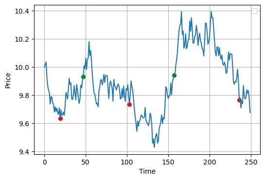
In this specific experiment, the parameters that define the Ornstein-Uhlenbeck (OU) process are set as follows: $\mu=10$, $\theta=10$, and $\sigma=1$. As depicted in Figure 2, the graph displays the trajectories of the 10 testing samples. The calculated average optimal stopping value is found to be 10.23. Importantly, the maxima for the majority of these paths are observed to cluster around 10.4, which lends credence to the computed optimal stopping value of 10.23. This result compellingly validates the effectiveness of our signature-based optimal stopping methodology, as it consistently produces high optimal stopping values for the simulated OU process.

Figure 2: The paths of the 10 testing samples.

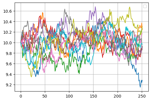
We have also executed a series of tests to examine the optimal stopping values generated by the signature method across a range of parameter combinations within the Ornstein-Uhlenbeck (OU) process. The aggregate findings of these tests are consolidated in Table 1. Significantly, all the optimal stopping values obtained exceeded the long-term mean of 10. A particularly insightful observation is the positive correlation between the optimal stopping value and the volatility parameter $\sigma$. This observed relationship underscores the sensitivity of the optimal stopping decision to the volatility of the underlying process, highlighting the nuanced interplay between process parameters and stopping outcomes.

$\mu$	$\sigma$	$\theta$	Optimal Stopping Value
1	1.0	10	10.1284
5	1.0	10	10.2311
10	1.0	10	10.2332
15	1.0	10	10.2005
20	1.0	10	10.1703
10	0.1	10	10.0025
10	0.5	10	10.0713
10	1.0	10	10.2264
10	1.5	10	10.3599
10	2.0	10	10.5173

Table 1: The optimal stopping value estimated by signature method on simulated mean-reversion process. Parameters $\mu\in\{1,5,10,15,20\}$ and $\sigma\in\{0.1,0.5,1.0,1.5,2.0\}$.

6.2 Signature-Based Optimal Trading Simulation

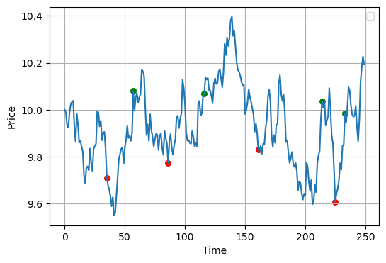
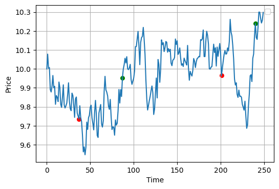
In this section, we conduct simulations using the Ornstein-Uhlenbeck (OU) process to test the effectiveness of our proposed optimal trading timing method for identifying both entry and exit times in mean-reverting markets. Specifically, we aim to evaluate the method introduced in Section 5, designed to yield sequential optimal entry and exit timings for a mean-reverting process. As in previous tests, we continue to assume that the mean-reversion process under consideration is governed by an Ornstein-Uhlenbeck (OU) model. This simulation study serves to validate the utility of our approach in generating actionable trading decisions based on the underlying stochastic process.

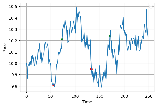
Figure 3 displays the performance of our simulation, where we have marked optimal entry times using red points and optimal exit times with green points. This color-coded representation provides an intuitive snapshot of how adeptly our method identifies strategic moments to both enter and exit trades in a mean-reverting market. As is evident from the graph, our method proves highly effective, consistently point times that align well with the natural peaks and troughs of the mean-reverting process. These results lend robust empirical support to the theoretical analysis of our proposed trading timing methodology, introduced in Section 5. Moreover, they offer compelling evidence that our approach can serve as a valuable tool for traders and portfolio managers seeking to exploit mean-reversion opportunities in financial markets. The simulation outcomes underscore the practical applicability and accuracy of our algorithm, confirming its utility for making well-informed, timely trading decisions based on the dynamics of the underlying stochastic process.

Figure 3: The sequential optimal entry and exit times for a simulated mean reversion process based on optimal trade timing framework.

6.3 Signature-Based Optimal Trading in Mean-Reverting Markets

In this section, we broaden the application of our signature-based optimal stopping methodology to a real-world trading context. Initially, we handpick four asset pairs from the financial markets to create their corresponding spreads. Utilizing the Ornstein-Uhlenbeck (OU) model as the underlying framework to describe these spreads, we then proceed to estimate the OU parameters for each pair. Equipped with these parameters, we generate respective OU samples and payoff processes, which facilitate the computation of an optimal linear function $l^{*}$ tailored to each pair.

It’s important to highlight that our method is highly adaptable and can accommodate various models for representing the underlying mean-reverting spreads. This includes but is not limited to exponential OU models and Cox-Ingersoll-Ross (CIR) models. By employing these models to characterize the constructed spreads, we can estimate the relevant parameters and generate training samples, ultimately yielding the optimal linear function for each specific trading scenario.

Once the optimal functions are determined, we implement the signature optimal stopping times as trading rules and assess their impact on trading performance. Our analysis then shifts focus to a comparative evaluation, where we juxtapose the trading performance achieved under our signature-based optimal trading strategy against the performance without such optimized entry and exit points. This examination provides a comprehensive view of the efficacy and practical applicability of our methodology in real-world trading situations.

In this segment, we elaborate on the specific securities employed to construct our asset pairs. We have selected four highly co-integrated stock pairs from diverse sectors within the U.S. market: WM-RSG from waste management, UAL-DAL from the airline industry, V-MA from financial services, and GS-MS from investment banking. A comprehensive description of these companies is provided in Table 2. Data pertaining to the daily closing prices for these stocks was collected for the period spanning January 1, 2021, to December 31, 2022. The data was sourced via the Yahoo! Finance API.

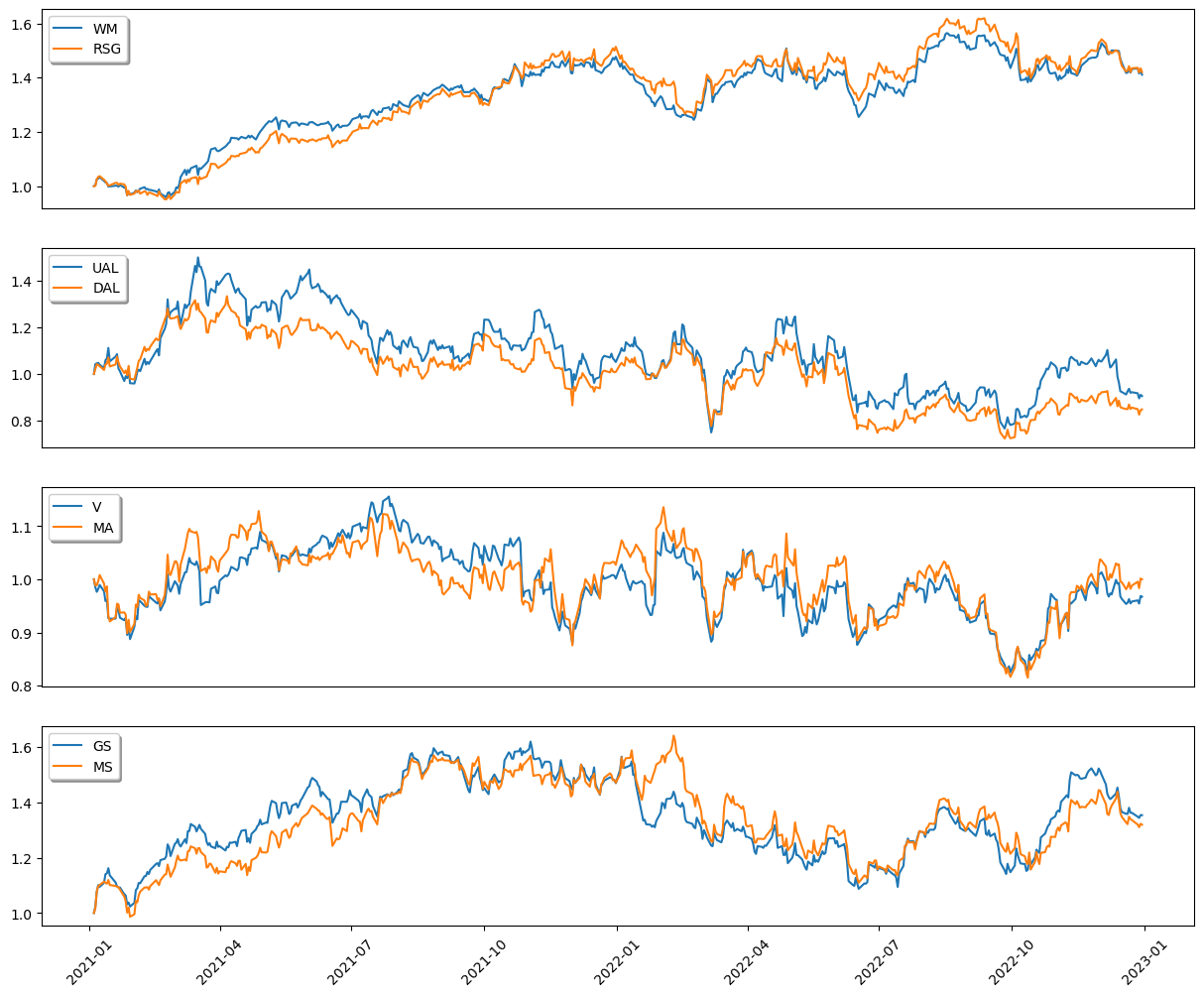
Figure 4 depicts the price trajectories of each stock pair, revealing a notable similarity in the price paths within each pair. For the sake of clarity and comparability, we have normalized each price series by dividing it by its respective initial value. This normalization allows for a more straightforward visual assessment of the relative movements between the stocks in each pair, thereby setting the stage for the forthcoming trading experiments.

Pairs Symbols	Description
WM-RSG	Waste Management and Republic Services provide waste management
	and environmental services
UAL-DAL	United Airlines and Delta Air Lines are two major American airline
	operating a large domestic and international route network.
V-MA	Visa and Mastercard are two large-cap stocks in the payment industry
GS-MS	Goldman Sachs and Morgan Stanley are American multinational investment bank
	and financial services company.

Table 2: The stock pairs used for testing and the description of the company.

Figure 4: Normalized historical daily close prices of six pairs of stocks from 1/1/2021–12/31/2022. From top to bottom: WM-RSG, UAL-DAL, V-MA, GS-MS, where each pair shows visibly persistent comovement.

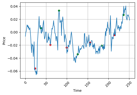
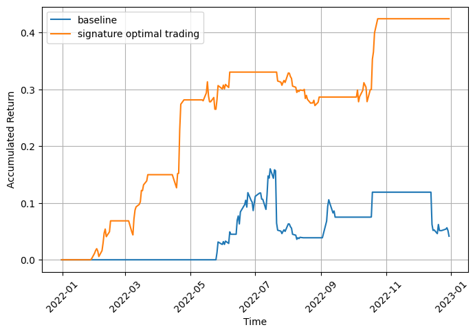
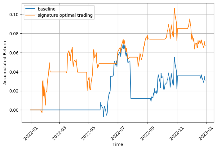
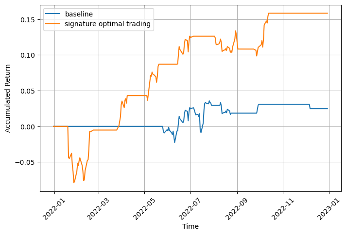
In the experiments, we simulated one full year of trading activity, as visually presented in Figure 5. Specifically, we created asset pairs based on the daily adjusted closing prices from the first year, covering a period of 252 trading days. These pairs were then actively traded over the course of the subsequent year. By doing so, we aim to evaluate the real-world applicability and effectiveness of our signature-based optimal stopping method within a time frame that captures a meaningful range of market conditions. This setup allows us to assess how well the trading rules, derived from the initial year’s data, generalize to unseen data in the following year. The hyper-parameters in our experiment is selected as $k=0.05$.

As illustrated in Figure 5, our algorithm excels in identifying the opportunities of trading, consistently entering positions at low prices and exiting at higher prices. This behavior serves as a compelling demonstration to the efficacy of our signature-based optimal trading strategy. This strong performance underscores the algorithm’s utility as a valuable tool for market participants seeking to exploit mean-reversion opportunities with optimized entry and exit timings.

(a) WM-RSG

(b) UAL-DAL

(c) V-MA

(d) GS-MS

Figure 5: The constructed spreads and optimal entry and exit time points. Red spot is entry point and Green spot is exit point.

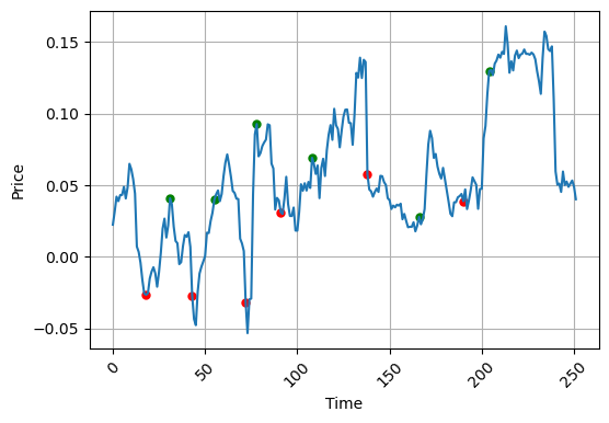
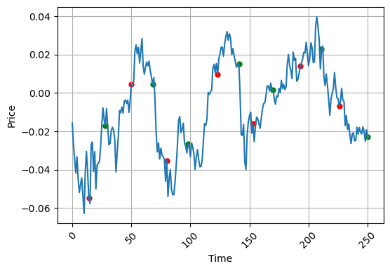
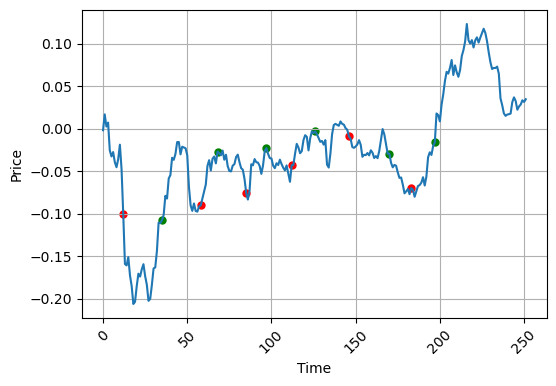
In the final phase of our analysis, we contrast the performance of our signature-based optimal trading strategy with a baseline strategy across all four asset pairs. The baseline strategy follows a simple rule: go long on $X_{t}$ when its price falls below $MA(X_{t})-k\times Std(X_{t})$, and liquidate the position when the price rises above $MA(X_{t})+k\times Std(X_{t})$. Here we write $MA(X_{t})$ and $Std(X_{t})$ to represent the moving average and standard deviation of past spread, respectively.

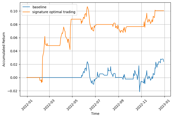
Table 3 presents a thorough comparison of performance metrics for both the baseline and the signature-based optimal trading (SOT) strategies. In this evaluation, the baseline strategy employs a constant $k$ value of 0.1 for its trading rules and leverages the preceding 100 samples to compute both the moving average and standard deviation. Figure 6 graphically illustrates the cumulative returns generated by each strategy over a one-year time frame.

As revealed by Table 3, our proposed signature-based optimal trading (SOT) strategy substantially outperforms the baseline model in key performance metrics, including higher cumulative returns and a more favorable daily Sharpe ratio. This head-to-head comparison is specifically tailored to underscore the superior efficacy of the SOT approach. It compellingly attests to the enhanced performance and incremental value that our method brings to the table in trading scenarios.

The visual representation of cumulative returns in Figure 6 serves as another pivotal element in our comparative assessment. It provides an intuitive snapshot of how the respective trading strategy compound over a one-year period. By offering this view, we further reinforce the idea that the SOT strategy is not only theoretically robust but also practically effective and adaptable to real-world market conditions. This comprehensive evaluation aims to highlight the enduring viability and real-world utility of the SOT methodology.

	WM/RSG		UAL/DAL		V/MA		GS/MS
	Baseline	SOT	Baseline	SOT	Baseline	SOT	Baseline	SOT
DailyRet ($\%$)	0.0110	0.0390	0.0401	0.1443	0.0107	0.0275	0.0119	0.0604
DailyStd ($\%$)	0.3513	0.4321	0.8244	0.8122	0.4177	0.5306	0.3362	0.5986
Sharpe	0.0313	0.0903	0.0487	0.1777	0.0255	0.0519	0.0354	0.1012
MaxDD ($\%$)	-1.9309	-0.7674	0	0	-0.7057	-0.2954	-2.2522	-7.9006
CumPnL ($\%$)	2.6363	10.0345	9.6431	42.4559	2.4857	6.7732	2.8829	15.8486
TradeNum	9	5	4	6	3	7	4	6

Table 3: Performance summary for all 4 pairs portfolios for baseline and the signature optimal trading (SOT). From the top to bottom rows, we report the annualized return, annualized standard deviation, Sharpe ratio, maximum drawdown and number of tradings.

(a) WM-RSG

(b) UAL-DAL

(c) V-MA

(d) GS-MS

Figure 6: The accumulative returns for baseline and SOT.

7 Conclusions

In this research paper, we have presented an innovative approach to identifying optimal timing strategies for trading price spreads with mean-reverting properties. Specifically, we formulated a sequential optimal stopping problem that accounts for the timing of both position entry and liquidation, while also incorporating transaction costs. To tackle this challenging problem, we employed the signature optimal stopping method, a powerful tool for determining the optimal entry and exit times that maximize trading returns.

Our approach is distinguished by its versatility: it is designed to adapt to a wide array of mean reversion dynamics, making it broadly applicable to a variety of trading scenarios. To validate the efficacy of our methodology, we carried out a comprehensive set of numerical experiments. These experiments served to compare the performance of our approach against conventional mean-reversion trading rules. The results consistently demonstrated the superior performance of our signature-based optimal trading strategy in terms of key metrics such as cumulative returns and Sharpe ratios.

In summary, this paper makes a significant contribution to the field of quantitative finance by introducing a robust and adaptable method for optimizing trading decisions in mean-reverting markets. Our findings affirm that the signature optimal stopping method offers not only theoretical rigor but also practical utility, presenting a compelling solution to a complex problem in finance. While our focus has been on specific asset pairs and trading conditions, the general principles and techniques introduced here have the potential for broader applications, opening up avenues for future research and practical implementations.

References

- Avellaneda and Lee [2010] Marco Avellaneda and Jeong-Hyun Lee. Statistical arbitrage in the us equities market. Quantitative Finance, 10(7):761–782, 2010.
- Bayer et al. [2021] Christian Bayer, Paul Hager, Sebastian Riedel, and John Schoenmakers. Optimal stopping with signatures. arXiv preprint arXiv:2105.00778, 2021.
- Brennan and Schwartz [1990] Michael J. Brennan and Eduardo S. Schwartz. Arbitrage in stock index futures. Journal of Business, 63(1):S7–S31, 1990.
- Dai et al. [2011] Min Dai, Yifei Zhong, and Yue Kuen Kwok. Optimal arbitrage strategies on stock index futures under position limits. Journal of Futures Markets, 31(4):394–406, 2011.
- d’Aspremont [2011] Alexandre d’Aspremont. Identifying small mean-reverting portfolios. Quantitative Finance, 11(3):351–364, 2011.
- Do and Faff [2012] Binh Do and Robert Faff. Are pairs trading profits robust to trading costs? Journal of Financial Research, 35(2):261–287, 2012.
- Do et al. [2006] Binh Do, Robert Faff, and Kais Hamza. A new approach to modeling and estimation for pairs trading. In Proceedings of 2006 financial management association European conference, volume 1, pages 87–99. Citeseer, 2006.
- Ekström et al. [2011] Erik Ekström, Carl Lindberg, and Johan Tysk. Optimal liquidation of a pairs trade. Advanced mathematical methods for finance, pages 247–255, 2011.
- Elliott et al. [2005] R.J. Elliott, J. Van Der Hoek, and W.P. Malcolm. Pairs trading. Quantitative Finance, 5(3):271–276, 2005.
- Engle and Granger [1987] Robert F Engle and Clive WJ Granger. Co-integration and error correction: representation, estimation, and testing. Econometrica, 55(2):251–276, 1987.
- Galenko et al. [2012] Alexander Galenko, Elmira Popova, and Ivilina Popova. Trading in the presence of cointegration. The Journal of Alternative Investments, 15(1):85–97, 2012.
- Gatev et al. [2006] Evan Gatev, William N Goetzmann, and K Geert Rouwenhorst. Pairs trading: Performance of a relative-value arbitrage rule. Review of Financial Studies, 19(3):797–827, 2006.
- Guijarro-Ordonez et al. [2021] Jorge Guijarro-Ordonez, Markus Pelger, and Greg Zanotti. Deep learning statistical arbitrage. Available at SSRN 3862004, 2021.
- Hambly and Lyons [2010] Ben Hambly and Terry Lyons. Uniqueness for the signature of a path of bounded variation and the reduced path group. Annals of Mathematics, pages 109–167, 2010.
- Huck and Afawubo [2015] Nicolas Huck and Komivi Afawubo. Pairs trading and selection methods: is cointegration superior? Applied Economics, 47(6):599–613, 2015.
- Kanamura et al. [2010] T. Kanamura, S.T. Rachev, and F.J. Fabozzi. A profit model for spread trading with an application to energy futures. The Journal of Trading, 5(1):48–62, 2010.
- Leung and Li [2015] Tim Leung and Xin Li. Optimal mean reversion trading with transaction costs and stop-loss exit. International Journal of Theoretical and Applied Finance, 18(03):1550020, 2015.
- Leung and Li [2016] Tim Leung and Xin Li. Optimal Mean Reversion Trading: Mathematical Analysis and Practical Applications. Modern Trends in Financial Engineering. World Scientific Publishing Company, 2016.
- Leung and Nguyen [2019] Tim Leung and Hung Nguyen. Constructing cointegrated cryptocurrency portfolios for statistical arbitrage. Studies in Economics and Finance, 2019.
- Leung et al. [2020] Tim Leung, Jize Zhang, and Aleksandr Aravkin. Sparse mean-reverting portfolios via penalized likelihood optimization. Automatica, 111:108651, 2020.
- Liew and Wu [2013] Rong Qi Liew and Yuan Wu. Pairs trading: A copula approach. Journal of Derivatives & Hedge Funds, 19(1):12–30, 2013.
- Montana and Triantafyllopoulos [2011] G. Montana and K. Triantafyllopoulos. Dynamic modeling of mean reverting spreads for statistical arbitrage. Computational Management Science, 8:23–49, 2011.
- Song et al. [2009] QS Song, George Yin, and Qing Zhang. Stochastic optimization methods for buying-low-and-selling-high strategies. Stochastic Analysis and Applications, 27(3):523–542, 2009.
- Vidyamurthy [2004] Ganapathy Vidyamurthy. Pairs Trading: quantitative methods and analysis, volume 217. John Wiley & Sons, 2004.
- Xie et al. [2016] Wenjun Xie, Rong Qi Liew, Yuan Wu, and Xi Zou. Pairs trading with copulas. The Journal of Trading, 11(3):41–52, 2016.