Cardinality Constrained Mean-Variance Portfolios:
A Penalty Decomposition Algorithm

Abstract

The cardinality-constrained mean-variance portfolio problem has garnered significant attention within contemporary finance due to its potential for achieving low risk while effectively managing risks and transaction costs. Instead of solving this problem directly, many existing methodologies rely on regularization and approximation techniques, which hinder investors’ ability to precisely specify the desired cardinality level of a portfolio. Moreover, these approaches typically include more hyper-parameters and increase problem dimensions. In response to these challenges, we demonstrate that a customized penalty decomposition algorithm is perfectly capable of tackling the original problem directly. This algorithm is not only convergent to a local minimizer but also is computationally cheap. It leverages a sequence of penalty subproblems where each of them is tackled via a block coordinate descent approach. In particular, the steps within the latter algorithm yield closed-form solutions and enable the identification of a saddle point of the penalty subproblem. Finally, through the application of our penalty decomposition algorithm to real-world datasets, we showcase its efficiency and its ability to outperform state-of-the-art methods in terms of CPU time.

1 Introduction

Mean-variance portfolio optimization is of paramount importance in finance, enabling investors to balance risk and return through strategic diversification [7]. On the other side, sparsity is a well-received property in mathematical optimization that has been proven to be advantageous in various subjects [14]. For example, leveraging sparsity has been proven crucial for efficient algorithms, allowing for more concise and computationally economical representations, particularly in tasks involving large-scale data [12]. This property becomes particularly relevant when applied to mean-variance portfolios, where promoting sparsity significantly reduces transaction costs [9]. Therefore, in this paper, we study the following cardinality-constrained mean-variance (CCMV) portfolio problem [13]:

$$\quad\min_{x\in\mathbb{R}^{n}}\ f(x):=x^{T}Ax-\tau\mu^{T}x\qquad\mbox{subject to}\qquad e^{T}x=1,\quad x\geq 0\quad\text{and}\quad\|x\|_{0}\leq k,$$ (1)

where $\tau>0$ balances the trade-off between minimizing risk and maximizing return, $\mu\in\mathbb{R}^{n}$ is the return vector, $A\succeq 0$ is the covariance matrix, and $k\in[n]$ is an upper bound for the number of desired assets.

Since it is well-established that sparsity can be promoted using convex or nonconvex regularization techniques [14], many state-of-the-art studies resort to such approaches and solve approximations of (1) [8, 2, 17]. However, this methodology is not favorable because it includes a regularization parameter that only implicitly controls the number of assets captured by that obtained portfolio (that is, the number of nonzero elements in the obtained solution). Further, this approach requires careful tuning of hyperparameters, which can be computationally expensive and challenging. Semidefinite relaxation methods are also proposed [10], but at least for medium or large-size problems are computationally expensive as the number of decision variables in their formulation is squared. Moreover, at present, they lack rigorous theoretical justification that clarifies how to interpret the results of the corresponding semidefinite program based on the original problem. Note that (1) can be recast as a mixed integer programming similar to approaches employed in [1, 4]. Nevertheless, this thrust requires an exhaustive search, making it practically not suitable for large-scale problems. Therefore, it is more advantageous to directly solve cardinality-constrained mean-variance portfolio problems rather than their approximations or regularized variations, where the practitioner has the choice to explicitly specify the number of assets in the portfolio [16].

To this point, for tackling (1) without the nonnegativity constraint, an ADMM method has been recently proposed [16]. However, in addition to requiring penalty parameter tuning, this method incorporates the equality constraint into the objective function by means of another positive parameter that also must be selected carefully in practice. Further, the obtained solution of this method does not satisfy the first-order necessary optimality conditions. [13] proposes an $\ell_{1}$-norm penalty alternating direction method (CCMV-PADM) for solving (1). This method resorts to solving a sequence of penalty subproblems that are tackled via a block coordinate descent approach. But, for each penalty parameter, this method requires solving a sequence of quadratic programs with a problem-sized number of linear constraints, which is expensive at least for large-size problems. Further, the obtained solution in this method (that is, the limit point of their sequence) is only a partial minimum. In other words, the solution cannot be improved in any of its decomposed parts (but it is not a local minimum of the problem).

To address these limitations, we present a customized penalty decomposition algorithm (CCMV-PD) designed to find a local minimizer of the optimization problem (1). Our approach also involves solving a series of penalty subproblems using a block coordinate descent algorithm, but notably, each subproblem within this framework has a closed-form solution, thus making it more computationally efficient compared to CCMV-PADM. Further, numerical evidence based on real data demonstrates the superior performance of our algorithm compared to CCMV-PADM based on a number of standard performance metrics and it is competitive with the commercial solver Mosek [6]. Further, we demonstrate that our proposed method CCMV-PD outperforms Mosek and CCMV-PADM in terms of CPU time.

Notation. We define the set $[n]$ as $\{1,2,\dots,n\}$ for any natural number $n$. The set complement of $S$ is represented as $S^{c}$. For a subset $S=\{i_{1},i_{2},\dots,i_{|S|}\}$, where $i_{k}$ are elements in $[n]$, and for any vector $x$ in $\mathbb{R}^{n}$, we define $x_{S}$ as the coordinate projection of $x$ with respect to the indices in set $S$. In other words, $(x_{S})_{i}=x_{i}$ for $i$ belonging to $S$, and consequently, by slightly abusing the notation, an $S$-supported vector can be shown as $[x_{S};0]$. We assess whether the matrix $A$ is positive semidefinite or positive definite using the symbols $A\succeq 0$ and $A\succ 0$, respectively. Also, $\lambda_{\min}(A)$ and $\lambda_{\max}(A)$ show the minimum and maximum eigenvalue of $A$, respectively.

2 A Penalty Decomposition Algorithm for CCMV and Its Convergence

We introduce our customized penalty decomposition method (CCMV-PD) for solving the cardinality-constrained mean-variance problem (1) and establish that it obtains a local minimizer of this nonconvex program.

2.1 CCMV-PD Algorithm

First, by introducing new variable $y$, we equivalently reformulate (1) as follows:

$$\min_{x,y\in\mathbb{R}^{n}}\quad x^{T}Ax-\tau\mu^{T}x\qquad\textrm{subject to}\qquad e^{T}x=1,\quad y\geq 0,\quad\|y\|_{0}\leq k,\quad\text{and}\quad x-y=0.$$ (2)

This splitting effectively handles the nonlinearly coupled constraints of the original problem. Suppose that

$$q_{\rho}(x,y):=x^{T}Ax-\tau\mu^{T}x+\rho\|x-y\|_{2}^{2},$$ (3)

and

$$\mathcal{X}:=\{x\in\mathbb{R}^{n}\,|\,e^{T}x=1\},\qquad\text{ and }\qquad\mathcal{Y}:=\{y\in\mathbb{R}^{n}\,|\,y\geq 0\quad\text{and}\quad\|y\|_{0}\leq k\}.$$

After penalizing the last constraint in (2), we consider a sequence of penalty subproblems as follows:

$$\min_{x,y\in\mathbb{R}^{n}}\quad q_{\rho}(x,y)\qquad\textrm{subject to}\qquad x\in\mathcal{X},\quad\text{ and }\quad y\in\mathcal{Y}.$$ (4)

To gain insights regarding the above formulation, it can be seen that by gradually increasing $\rho$ toward infinity, we can effectively address the optimization problem (2). The introduction of the auxiliary variable $y$ is designed to simplify the subproblems encountered when implementing the subsequent algorithm for obtaining a saddle point in (4).

Algorithm 1 BCD Algorithm for Solving (4)

1:  Input: Select arbitrary $y_{0}\in\mathcal{Y}$.

2:  Set $l=0$.

3:  repeat

4:     $x_{l+1}=\mbox{Argmin}_{x\in\mathcal{X}}\ q_{\rho}(x,y_{l}).$

5:     $y_{l+1}=\mbox{Argmin}_{y\in\mathcal{Y}}\ q_{\rho}(x_{l+1},y).$

6:     $l\leftarrow l+1$ and go to step (3).

7:  until stopping criterion (5) is met.

Our stopping criterion for this BCD loop is the following:

$$\max\left\{\frac{\|x_{l}-x_{l-1}\|_{\infty}}{\max\left(\|x_{l}\|_{\infty},1\right)},\frac{\|y_{l}-y_{l-1}\|_{\infty}}{\max\left(\|y_{l}\|_{\infty},1\right)}\right\}\leq\epsilon_{I}.$$ (5)

We next study how to efficiently solve the restricted subproblems in Algorithm 1 below.
$\bullet\ \mbox{Argmin}_{x\in\mathcal{X}}\ q_{\rho}(x,y)$: This subproblem becomes the following convex quadratic optimization problem:

$$\min_{x\in\mathbb{R}^{n}} x^{T}Ax-\tau\mu^{T}x+\rho\|x-y\|^{2}\qquad\textrm{subject to}\qquad e^{T}x=1.$$ (6)

Since $A\succeq 0$ and $\rho>0$, we have $A+\rho I\succ 0$. Hence, this feasible problem has a solution and its KKT conditions are as follows:

$$2Ax_{*}-\tau\mu+2\rho(x_{*}-y)+\beta e=0,\quad\mbox{ and }\quad e^{T}x_{*}=1.$$

Thus, $2(A+\rho I)x_{*}=\tau\mu+2\rho y-\beta e$ implies $x_{*}=0.5(A+\rho I)^{-1}(\tau\mu+2\rho y-\beta e)$. Since $1=e^{T}x_{*}=0.5e^{T}(A+\rho I)^{-1}(\tau\mu+2\rho y-\beta e)$, we get

$$\beta=\frac{-1+0.5e^{T}(A+\rho I)^{-1}(\tau\mu+2\rho y)}{0.5e^{T}(A+\rho I)^{-1}e},$$

which in turn yields

$$x_{*}=\frac{1}{2}(A+\rho I)^{-1}\left(\tau\mu+2\rho y-\frac{1-0.5e^{T}(A+\rho I)^{-1}(\tau\mu+2\rho y)}{0.5e^{T}(A+\rho I)^{-1}e}e\right)$$ (7)

$\bullet\ \mbox{Argmin}_{y\in\mathcal{Y}}\ q_{\rho}(x,y)$: This subproblem is as follows:

$$\min_{y\in\mathbb{R}^{n}}\ \|x-y\|_{2}^{2}\qquad\mbox{subject to}\qquad y\geq 0,\quad\textrm{and}\quad\|y\|_{0}\leq k.$$ (8)

Recall that for $x\in\mathbb{R}$ and $k\in\mathbb{N}$, the sparsifying operator $H_{k}(x):=[x_{\mathcal{J}};0]$, where $\mathcal{J}=\mathcal{J}(x,k)$ is an index set corresponding to the $k$ largest components of $x$ in absolute value.

Lemma 2.1.

The solution of the above problem (8) is

$$y_{*}=H_{k}(x^{+})=H_{k}(\max(x,0)).$$ (9)

We highlight that when compared to the subproblems discussed above, the subproblems in the penalty alternative direction method (CCMV-PADM) are different and given by:

$$\min_{x\in\mathbb{R}^{n}}\quad x^{T}Ax-\tau\mu^{T}x+\rho\|x-y\|_{1}\qquad\textrm{subject to}\qquad e^{T}x=1,\quad\text{and}\quad x\geq 0,$$

and

$$\begin{aligned} \min_{y\in\mathbb{R}^{n}}\quad\|x-y\|_{1}\qquad\textrm{subject to}\qquad e^{T}y=1,\quad\text{and}\quad\|y\|_{0}\leq k,\end{aligned}.$$

Note that the former is equivalent to a quadratic program with $n$ constraints. Solving this subproblem becomes more expensive (recall that this is being solved iteratively) as the size of the problem increases. Additionally, CCMV-PADM only captures a partial minimum of the problem (1), not a local minimum.

To address these drawbacks, we introduce the CCMV penalty decomposition (CCMV-PD) algorithm. It starts with a positive penalty parameter and incrementally enlarges it until a convergence result is achieved. For a fixed $\rho$, Algorithm 1 handles the corresponding subproblem. Note that (1) is feasible, and we assume the availability of a feasible point denoted as $x^{\text{feas}}$. To facilitate the presentation of this algorithm and its subsequent analysis, we introduce the following notation:

$$\Upsilon\geq\max\{f(x^{\text{feas}}),\min_{x\in\mathcal{X}}q_{\rho^{(0)}}(x,y^{(0)}_{0})\}>0\qquad\text{ and }\qquad X_{\Upsilon}:=\{x\in\mathbb{R}^{n}\,|\,f(x)\leq\Upsilon\}.$$ (10)

Furthermore, since $A\succeq 0,$ it is evident from a normalization argument that $X_{\Upsilon}$ is bounded and, therefore, compact.

Algorithm 2 CCMV-PD Algorithm for Solving (1)

1:  Inputs: $\zeta>1,\rho^{(0)}>0$, and $y^{(0)}_{0}\in\mathcal{Y}$.

2:  Set $j=0$.

3:  repeat

4:     Set $l=0$.

5:     repeat

6:        Solve $x^{(j)}_{l+1}=\mbox{Argmin}_{x\in\mathcal{X}}\ q_{\rho}(x,y^{(j)}_{l}).$

7:        Solve $y^{(j)}_{l+1}\in\mbox{Argmin}_{y\in\mathcal{Y}}\ q_{\rho}(x^{(j)}_{l+1},y).$

8:        Set $l\leftarrow l+1$.

9:     until stopping criterion (5) is met.

10:     Set $(x^{(j)},y^{(j)}):=(x^{(j)}_{l},y^{(j)}_{l})$.

11:     Set $\rho^{(j+1)}=\zeta\cdot\rho^{(j)}$.

12:     If $\min_{x\in\mathcal{X}}q_{\rho^{(j+1)}}(x,y^{(j)}_{l})>\Upsilon$, then $y_{0}^{(j+1)}=x^{\text{feas}}$. Otherwise, $y^{(j+1)}_{0}=y^{(j)}_{l}$.

13:     Set $j\leftarrow j+1$.

14:  until stopping criterion (11) is met.

The convergence of the outer loop is met when:

$$\|x^{(j)}-y^{(j)}\|_{\infty}\leq\epsilon_{O}.$$ (11)

2.2 Convergence Analysis of CCMV-PD Algorithm

We begin by examining Algorithm 1 and subsequently establish the desirable properties of Algorithm 2. We conduct an analysis of a sequence $\{(x_{l},y_{l})\}$ generated by Algorithm 1, demonstrating that any sequence within it attains a saddle point of (4):

$$x_{*}\in\mbox{Argmin}_{x\in\mathcal{X}}\ q_{\rho}(x,y_{*}),\qquad\mbox{ and }\qquad y_{*}\in\mbox{Argmin}_{y\in\mathcal{Y}}\ q_{\rho}(x_{*},y).$$

This shows the reason for choosing a block coordinate descent (BCD) scheme for this nonconvex problem.

Lemma 2.2.

Let $\tau\in\mathbb{R},A\succ 0,$ and $\rho\geq 1+\lambda_{\max}(A)$. Consider the BCD iterates, that is, $x_{l}\in\mbox{Argmin}_{x\in\mathcal{X}}\ q_{\rho}(x,y_{l-1})$, $y_{l}\in\mbox{Argmin}_{y\in\mathcal{Y}}\ q_{\rho}(x_{l},y)$, we get

$$\max\{\|x_{l}\|,\|y_{l}\|\}\leq\frac{(\tau+2\lambda_{\max}(A))\|\mu\|}{2+2\lambda_{\max}(A)}=:\kappa.$$ (12)

The above lemma shows that the sequence created by Algorithm 1 is bounded, implying that every sequence generated by this algorithm obtains an accumulation point. The next theorem proves that every accumulation point is a saddle point of (4). Additionally, the sequence $(q_{\rho}(x_{l},y_{l}))$ is either strictly decreasing or two consecutive terms produce the same value, resulting in a saddle point. Essentially, Algorithm 1 produces a saddle point either in finite steps or in the limit.

Theorem 2.1.

Let $\rho>0$. Consider the sequence $\{(x_{l},y_{l})\}$ generated by Algorithm 1 to solve (4). If $(x_{*},y_{*})$ is an accumulation point of this sequence, then $(x_{*},y_{*})$ is a saddle point of the non-convex problem (4). Additionally, the sequence $\left\{q_{\rho}(x_{l},y_{l})\right\}$ is non-increasing, and if $q_{\rho}(x_{r},y_{r})=q_{\rho}(x_{r+1},y_{r+1})$ for some $r\in\mathbb{N}$, then $(x_{r},y_{r})$ is a saddle point of (4).

Assuming that $x^{*}$ is a local minimum of (1), there exists an index set $\mathcal{L}$ such that $|\mathcal{L}|=k$ and $x^{*}_{\mathcal{L}^{c}}=0$ such that $x^{*}$ is also a local minimizer of the following problem:

$$\min_{x\in\mathbb{R}^{n}}\ x^{T}Ax-\tau\mu^{T}x\qquad\mbox{subject to}\qquad e^{T}x=1,\quad x\geq 0,\quad\text{and}\quad x_{\mathcal{L}^{c}}=0.$$ (13)

Robinson’s constraint qualification condition for a local minimizer $x^{*}$ of (13) is [15]:

$$\left\{\begin{bmatrix}-d-v\\ e^{T}d\\ d_{\mathcal{L}^{c}}\end{bmatrix}\ \Big{|}\ \ d\in\mathbb{R}^{n},\ \ v\in\mathbb{R}^{n},\ \ v_{i}\leq 0;\,\forall i\in\mathcal{L}^{c}\right\}=\mathbb{R}^{n}\times\mathbb{R}\times\mathbb{R}^{|\mathcal{L}^{c}|}.$$ (14)

It is easy to show that Robinson’s conditions above always hold for an arbitrary $x^{*}$. Therefore, the KKT conditions for a local minimizer $x^{*}$ of (1) holds, which are the existence of $(\lambda,\mu,w)\in\mathbb{R}^{n}\times\mathbb{R}\times\mathbb{R}^{n}$ and $\mathcal{L}\subseteq[n]$ with $|\mathcal{L}|=k$ such that the following holds:

$$2Ax-\tau\mu-\lambda+w+\beta e=0,\quad 0\leq\lambda\perp x\geq 0,\quad e^{T}x=1,\quad x_{{\mathcal{L}}^{c}}=0,\quad w_{\mathcal{L}}=0.$$ (15)

Now, we analyze a sequence $\left\{\left(x^{(j)},y^{(j)}\right)\right\}$ generated by Algorithm 2 and demonstrate that it finds a KKT point of (1).

Theorem 2.2.

Suppose that $\tau\in\mathbb{R},k\in[n],A\succeq 0$, and $\rho^{(0)}\geq\lambda_{\max}(A)+1$. Let $\left\{\left(x^{(j)},y^{(j)}\right)\right\}$ be a sequence generated by Algorithm 2 for solving (1). Then, the following hold:

• $\left\{\left(x^{(j)},y^{(j)}\right)\right\}$ has a convergent subsequence whose accumulation point $(x^{*},y^{*})$ satisfies $x^{*}=y^{*}$. Further, there exists an index subset $\mathcal{L}\subseteq[n]$ with $|\mathcal{L}|=k$ such that $x^{*}_{\mathcal{L}^{c}}=0$ and $x^{*}_{\mathcal{L}}\geq 0$.

• Let $x^{*}$ and $\mathcal{L}$ be defined above. Then, $x^{*}$ is a local minimizer of (1).

3 Numerical Results

In this section, we first compare the performance of CCVM-PD (2) for solving (1) with CCMV-PADM proposed in [13] and the commercial solver Mosek available in CVX [5] in terms of in-sample and out-of-sample returns, risks, and Sharpe ratios over the S&P index. We consider the period $2016-2020$ and randomly select $133$ stocks. For the out-of-sample performance, we apply the rolling-horizon procedure [3]. The formula for calculating the in-sample Sharpe ratio is ${SR}={\mu}/{\sigma},$ where $\mu$ is expected portfolio return and $\sigma$ is the standard deviation of portfolio and the out-of-sample Sharpe ratio ($\widehat{SR}$) is as follows:

$$\widehat{SR}=\dfrac{\widehat{\mu}}{\widehat{\sigma}},\qquad\text{ with }\qquad\widehat{\mu}=\dfrac{1}{T-\nu}\sum_{t=\nu}^{T-1}~{}(x_{t}^{T}~{}r_{t+1})\qquad\text{ and }\qquad\widehat{\sigma}^{2}=\dfrac{1}{T-\nu-1}\sum_{t=\nu}^{T-1}~{}(x_{t}^{T}~{}r_{t+1}-\widehat{\mu})^{2},$$

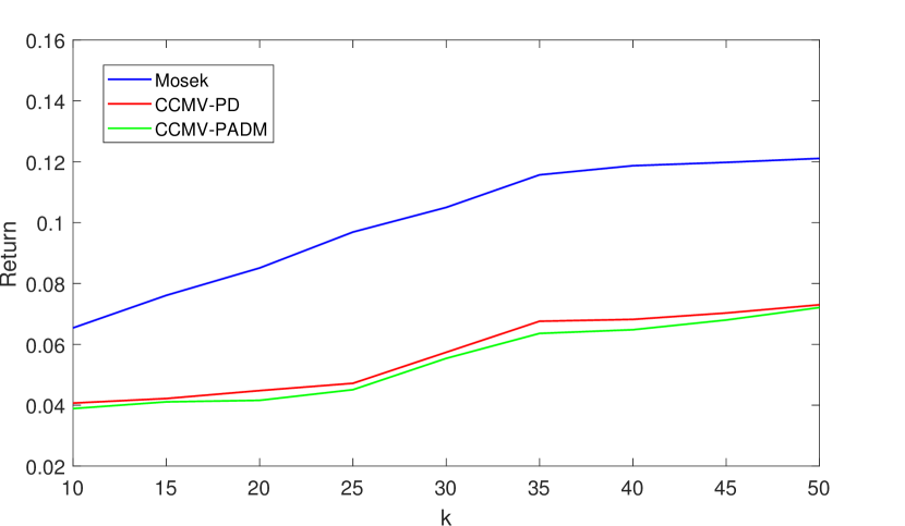
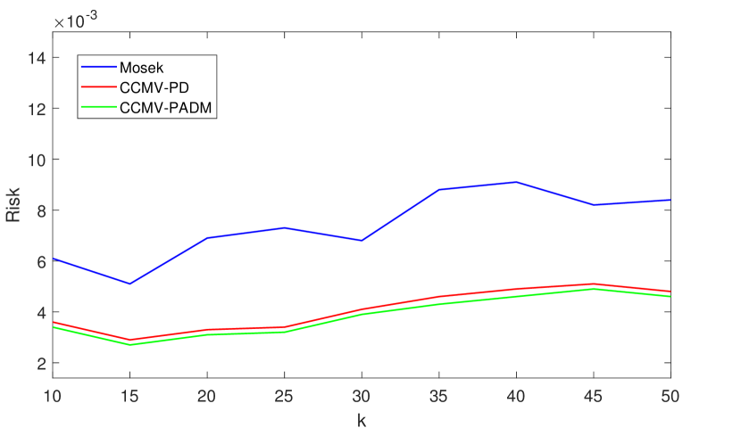
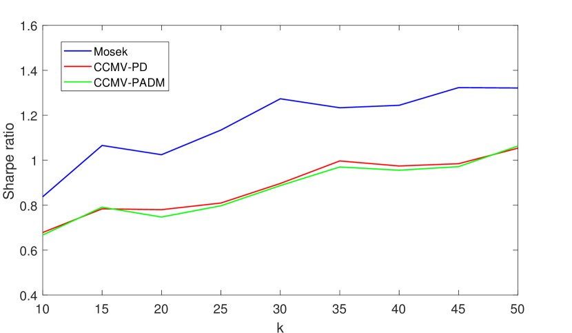
where $x_{t}$ denotes the stock weight at time $t$, and $T$ is the total number of returns in the dataset, $r_{t+1}$ is the stock return, and $\nu$ is the length of the estimation time window. By considering the monthly return of stocks from $2016$ to $2019$ and an estimation window of $\nu=48$ data, for $4$ years, we use the 2020 data for the out-of-sample. The results are summarized in Table 1 for when $n=133,\tau=0.5,\rho_{0}=0.1,\zeta=10$ and different values of $k$ are considered. We compare the performance of Algorithm 2 in terms of returns, risks, and Sharpe ratios for the model (1) with Mosek and CCMV-PADM for the dataset of S&P index from 2016 until 2019 when $T=60$. The BCD loop is stopped when $\epsilon_{I}=10^{-4}$ in (5). Algorithm 2 also terminates if $\epsilon_{o}=10^{-4}$ in (11). The results are summarized in Table 1. In this table, the gaps in the last three columns are ${|g-\widehat{g}|}/({|\widehat{g}|+1}),$ where $g$ and $\widehat{g}$ are the return, risk, Sharpe ratio of Mosek, CCMV-PD, and CCMV-PADM respectively.

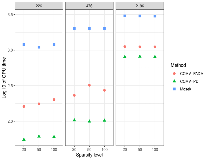
Our results reveal that CCMV-PD and CCMV-PADM overall have close returns, risks, and Sharpe ratios, however, our proposed method does significantly better in a time comparison. Further, for small sparsity levels, this closeness of Mosek and CCMV-PD is significant. These results can be further confirmed in the graphs of Figure 2. As one can see, from the results of out-of-sample in Table 1, the return, risk, and Sharpe ratio of all used methods in solving (1) are close to each other, which can be seen in the small gaps of these models. Secondly, we compare the performance of Algorithm 2 in terms of CPU time for the model (1) with Mosek and CCMV-PADM on the dataset of MIBTEL, S&P, and NASDAQ indexes for different values of $k$. These results are reported in Figure 1 and Table 2 and show that CCMV-PD solves (1) significantly faster and has smaller gaps. Due to the lack of space in this table, we shortened the return gap to re gap, risk gap to ri gap, and Sharpe ratio to Sr. We conclude that the results of CCMV-PD are competitive to the results of the solving model (1) by Mosek in CVX. Further, our method shows a better performance than CCMV-PADM overall.

Figure 1: Comparison of log10 of CPU times in Table 2 against sparsity level for $n=226,476,$ and $2196$.

Figure 2: Gap returns, risks, and Sharpe ratios for Mosek, CCPV-PD, and CCMV-PADM in solving (1) against sparsity level $k$.

	Mosek			CCMV-PD						CCMV-PADM
$k$	return	risk	Sr	return	risk	Sr	re gap	ri gap	Sr gap	return	risk	Sr	re gap	ri gap	Sr gap
20	0.0840	0.0051	1.1765	0.0663	0.0038	1.0755	0.0163	0.0013	0.0464	0.0654	0.0038	1.0609	0.0172	0.0013	0.0531
30	0.0808	0.0078	0.9151	0.0477	0.0020	0.6194	0.0306	0.0058	0.1544	0.0372	0.0038	0.4412	0.2500	0.0020	0.2475
40	0.0838	0.0053	1.1512	0.0441	0.0024	0.9002	0.0366	0.0028	0.1167	0.0428	0.0029	0.6035	0.0378	0.0024	0.1657
50	0.1087	0.0088	1.1589	0.0456	0.0027	0.8776	0.0569	0.0061	0.1303	0.0448	0.0031	0.8046	0.0576	0.0057	0.1641
20	0.1615	0.0082	1.7835	0.0653	0.0035	1.1038	0.0828	0.0048	0.2442	0.0651	0.0035	1.1004	0.0830	0.0047	0.2454
30	0.1609	0.0068	1.9512	0.0651	0.0031	1.1694	0.0825	0.0037	0.2649	0.0646	0.0031	1.1603	0.0829	0.0037	0.2680
40	0.1831	0.0087	1.9630	0.0669	0.0037	1.0998	0.0982	0.0051	0.2913	0.0651	0.0039	1.0424	0.0997	0.0048	0.3107
50	0.1836	0.0089	1.9462	0.0678	0.0041	1.0589	0.0978	0.0049	0.3012	0.0666	0.0040	1.0530	0.0989	0.0049	0.3032

Table 1: Comparison of returns, risks, and Sharpe ratios of Mosek, CCMV-PD, and CCMV-PADM for different sparsity levels when $n=133$

		Mosek
	$k$	return	risk	Sr	time
	20	0.0341	0.0028	0.6364	1.201e+03
$n=226$	50	0.0368	0.0035	0.6221	1.101e+03
	100	0.0432	0.0051	0.6049	1.1982e+03
	20	0.0328	0.0030	0.5965	$>$2.021e+03
$n=476$	50	0.0550	0.0045	0.8213	$>$2.018e+03
	100	0.0583	0.0052	0.8085	$>$2.014e+03
	20	0.0615	0.0065	0.7631	$>$3.031e+03
$n=2196$	50	0.0623	0.0066	0.7669	$>$3.024e+03
	100	0.0645	0.0069	0.6515	$>$3.015e+03

CCMV-PD							CCMV-PADM
return	risk	Sr	time	re gap	ri gap	Sr gap	return	risk	Sr	time	re gap	ri gap	Sr gap
0.0098	4.9697e-04	0.4434	55.1256	0.0234	0.0023	0.1179	0.0091	4.3275e-04	0.4374	161.324	0.0242	0.0024	0.1216
0.0125	4.7697e-03	0.1810	61.0236	0.0177	0.0014	0.2719	0.0118	4.2994e-03	0.1800	175.454	0.0224	7.9661e-04	0.2725
0.0187	1.6697e-03	0.4576	60.3265	0.0234	0.0034	0.0918	0.0181	2.2881e-04	0.4562	201.345	0.0241	0.0048	0.0927
0.0208	4.5780e-03	0.3074	103.1256	0.0116	0.0016	0.1811	0.0198	4.1776e-03	0.3063	231.304	0.0126	0.0012	0.1818
0.0215	0.0065	0.2667	99.1325	0.0318	0.0020	0.3045	0.0201	0.0061	0.2574	321.104	0.0331	0.0016	0.3096
0.0288	6.6639e-03	0.3528	102.1595	0.0279	0.0015	0.2520	0.0281	6.3839e-03	0.3517	272.326	0.0285	0.0013	0.2526
0.0266	0.0098	0.2687	803.1132	0.0329	0.0033	0.2804	0.0256	0.0096	0.2613	1.121e+03	0.0338	0.0031	0.2846
0.0267	9.8785e-03	0.2686	812.1335	0.0468	0.0033	0.2820	0.0105	9.5669e-03	0.2678	1.112e+03	0.0478	0.0029	0.2825
0.0123	9.8955e-03	0.4762	804.1635	0.0490	0.0092	0.1061	0.0118	9.2697e-04	0.4522	1.111e+03	0.0495	0.0092	0.1207

Table 2: Comparison of returns, risks, Sharpe ratios, and CPU times of Mosek, CCMV-PD, and CCMV-PADM in solving (1) for different numbers of stocks: $226$ stocks of MIBTEL, $476$ stocks of S&P, and $2196$ stocks of NASDAQ indexes.

4 Appendix

Technical proofs are given below.

4.1 Proof of Lemma 2.1

Proof.

Note that for any $y$ satisfying $\|y\|_{0}\leq k$, one can write $y=(y_{\mathcal{I}},y_{\mathcal{I}^{c}})$ such that $y_{\mathcal{I}}=0$ for some index set $\mathcal{I}\subseteq\{1,\ldots,n\}$ with $|\mathcal{I}|=n-k$. Hence, for any index set $\mathcal{I}$ with $|\mathcal{I}|=n-k$, $(P_{y})$ can be written as

$$\min_{y\in\mathbb{R}^{n}}(\|x_{\mathcal{I}}-y_{\mathcal{I}}\|^{2}_{2}+\|x_{\mathcal{I}^{c}}-y_{\mathcal{I}^{c}}\|^{2}_{2})\quad\text{subject to }\quad y\geq 0\quad\text{ and }\quad y_{\mathcal{I}}=0,$$

which is equivalent to

$$\min_{z\in\mathbb{R}^{|\mathcal{I}^{c}|}}\|z-x_{\mathcal{I}^{c}}\|^{2}_{2}\quad\text{subject to}\quad z\geq 0.$$

Clearly, constraint qualification holds, and its KKT condition for a local minimizer $z_{*}$ is: $x_{\mathcal{I}^{c}}=z_{*}-\lambda$ and $z_{*}\geq 0$ for some $\lambda\geq 0$ with $z_{*}^{T}\lambda=0$. Suppose that $x_{\mathcal{I}^{c}}=x^{+}_{\mathcal{I}^{c}}-x^{-}_{\mathcal{I}^{c}}$ such that $x^{+}_{\mathcal{I}^{c}}=\max(x_{\mathcal{I}^{c}},0)$ and $x^{-}_{\mathcal{I}^{c}}=\max(-x_{\mathcal{I}^{c}},0)$, then $x^{+}_{\mathcal{I}^{c}}\perp x^{-}_{\mathcal{I}^{c}}$. It is easy to see that $z_{*}=x^{+}_{\mathcal{I}^{c}}$ and $\lambda=x^{-}_{\mathcal{I}^{c}}$ satisfy the KKT conditions. Hence, it is easy to show that $z_{*}=x^{+}_{\mathcal{I}^{c}}$ for any index $\mathcal{I}$ specified above. Finally, for any index $\mathcal{I}$ specified above, the optimal value is given by $\|x_{\mathcal{I}^{c}}-x^{+}_{\mathcal{I}^{c}}\|^{2}_{2}+\|x_{\mathcal{I}}\|_{2}^{2}=\|x^{-}_{\mathcal{I}^{c}}\|^{2}_{2}+\|x_{\mathcal{I}}\|^{2}_{2}=\|x_{\mathcal{I}^{c}}\|_{2}^{2}-\|x^{+}_{\mathcal{I}^{c}}\|^{2}_{2}+\|x_{\mathcal{I}}\|^{2}_{2}=\|x\|_{2}^{2}-\|x^{+}_{\mathcal{I}^{c}}\|^{2}_{2}$. Consequently, the minimal value of $(P_{y})$ is achieved when $\|x^{+}_{\mathcal{I}^{c}}\|_{2}$ is maximal or equivalently when $\mathcal{I}^{c}=\mathcal{J}(x,k)=\mathcal{J}$. Therefore, a minimizer $y^{*}$ satisfies $y_{\mathcal{J}}=H_{k}(x^{+})=H_{k}(\max(x,0))$. ∎

4.2 Proof of Lemma 2.2

Proof.

By denoting $B=A+\rho I$ and $\alpha=0.5e^{T}B^{-1}e$, we see that $\|B^{-1}\|={1}/{{\lambda_{\min}(B)}}={1}/{({\lambda_{\min}(A)+\rho)}}\leq 1/{\rho}$, and ${n}/{\lambda_{\max(A)}}\leq{n}/{(\lambda_{\max}(A)+\rho)}={\|e\|^{2}}/{\lambda_{\max}(B)}=\|e\|^{2}\lambda_{\min}(B^{-1})\leq 2\alpha$. Thus, the equation (7) together with $\|y\|=\|H_{k}(x^{+})\|\leq\|x\|$ leads to

$$\|x\| \leq\frac{1}{2}\|B^{-1}\|\left(\tau\|\mu\|+2\rho\|y\|+\frac{\mu+\rho|e^{T}B^{-1}y|}{\alpha}\|e\|\right)$$

$$\leq\frac{1}{2\rho}\left(\tau\|\mu\|+2\rho\|y\|+2n^{-1}\lambda_{\max}(A)\|e\|\left(\|\mu\|+\|e\|\|y\|\right)\right)$$

$$=\frac{1}{2\rho}(\tau+2n^{-1}\lambda_{\max}(A)\|e\|)\|\mu\|+\frac{1}{2\rho}(1+2\lambda_{\max}(A))\|y\|$$

$$\leq\frac{1}{2\rho}(\tau+2n^{-1/2}\lambda_{\max}(A))\|\mu\|+\frac{1}{2\rho}(1+2\lambda_{\max}(A))\|x\|$$

Thus, whenever $\rho\geq 1+\lambda_{\max}(A),$ we have

$$\|x\|\leq\frac{\frac{1}{2\rho}(\tau+2n^{-1/2}\lambda_{\max}(A))\|\mu\|}{1-\frac{1}{2\rho}(1+2\lambda_{\max}(A))}\leq\frac{(\tau+2\lambda_{\max}(A))\|\mu\|}{2+2\lambda_{\max}(A)}.$$

∎

4.3 Proof of Theorem 2.1

Proof.

By observing definitions of $x_{l+1}$ and $y_{l+1}$ in steps 4 and 5 of Algorithm 1, we get

$$q_{\rho}(x_{l+1},y_{l+1}) \leq q_{\rho}(x_{l+1},y),\quad\forall y\in\mathcal{Y},$$

$$q_{\rho}(x_{l+1},y_{l}) \leq q_{\rho}(x,y_{l}),\quad\forall x\in\mathcal{X}.$$ (16)

This simply leads to the following:

$$c^{*} \leq q_{\rho}(x_{l+1},y_{l+1})\leq q_{\rho}(x_{l+1},y_{l})\leq q_{\rho}(x_{l},y_{l}),\quad\forall l\in\mathbb{N},$$ (17)

where $c^{*}=\min_{x}x^{T}Ax-\tau\mu^{T}x$ which is finite because $A\succ 0$. Thus, $q_{\rho}(x_{l},y_{l})$ is a bounded below and non-increasing sequence; implying that $q_{\rho}(x_{l},y_{l})$ is convergent. From the other side, since $(x_{*},y_{*})$ is an accumulation point of $\{(x_{l},y_{l})\}$, there exists a subsequence $L$ such that $\lim_{l\in L\to\infty}(x_{l},y_{l})=(x_{*},y_{*})$. The continuity of $q_{\rho}(x_{l},y_{l})$ yields

$$\lim_{l\to\infty}q_{\rho}(x_{l+1},y_{l+1}) =\lim_{l\to\infty}q_{\rho}(x_{l+1},y_{l})$$

$$=\lim_{l\to\infty}q_{\rho}(x_{l},y_{l})$$

$$=\lim_{l\in L\to\infty}q_{\rho}(x_{l},y_{l})$$

$$=q_{\rho}(x_{*},y_{*}).$$

By the continuity of $q_{\rho}(x_{l},y_{l})$ and taking the limit of both sides of (4.3) as $l\in L\to\infty$, we have

$$q_{\rho}(x_{*},y_{*})\leq q_{\rho}(x,y_{*}),\quad\forall x\in\mathcal{X},\quad\mbox{and}\quad q_{\rho}(x_{*},y_{*})\leq q_{\rho}(x_{*},y),\quad\forall y\in\mathcal{Y}.$$

Further, it is clear from (17) that $\left\{q_{\rho}(x_{l},y_{l})\right\}$ is non-increasing.

Next, suppose $q_{\rho}(x_{r},y_{r})=q_{\rho}(x_{r+1},y_{r+1})$ for some $r\in\mathbb{N}$. Then by (4.3), we have $q_{\rho}(x_{r+1},y_{r})=q_{\rho}(x_{r},y_{r})$. Furthermore, since $x_{r+1}\in\mathrm{Argmin}_{x\in\mathcal{X}}\ q_{\rho}(x,y_{r})$, we see $q_{\rho}(x_{r+1},y_{r})=\min_{x\in\mathcal{X}}q_{\rho}(x,y_{r})$. In view of $q_{\rho}(x_{r+1},y_{r})=q_{\rho}(x_{r},y_{r})$ and $x_{r}\in\mathcal{X}$, we have $q_{\rho}(x_{r},y_{r})=\min_{x\in\mathcal{X}}q_{\rho}(x,y_{r})$ such that $x_{r}\in\mathrm{Argmin}_{x\in\mathcal{X}}\ q_{\rho}(x,y_{r})$. Further, $y_{r}\in\mathcal{Y}$ satisfies $y_{r}\in\mathrm{Argmin}_{y\in\mathcal{Y}}\ q_{\rho}(x_{r},y)$. This shows that $(x_{r},y_{r})$ is a saddle point of $(P_{x,y})$.

∎

4.4 Proof of Theorem 2.2

Proof.

(i) By Lemma 2.2, we know that $\|y^{(j)}\|\leq\|x^{(j)}\|\leq\kappa$ defined in (12), for every $j\in\mathbb{N}$ whenever $\rho^{(j)}\geq\lambda_{\max}(A)+1$. Thus, $\{(x^{(j)},y^{(j)}\}$ is bounded and therefore, has a convergent subsequence. For our purposes, without loss of generality, we suppose that the sequence itself is convergent. Let $\left(x^{*},y^{*}\right)$ be its accumulation point. First, let us show that $x^{*}=y^{*}$. In view of definition (3), the step 12 of Algorithm 2, we have $f(x^{(j)})+\rho^{(j)}\|x^{(j)}-y^{(j)}\|_{2}^{2}\leq\min_{x\in\mathcal{X}}q_{\rho^{(j)}}(x,y_{0}^{(j)})\leq\Upsilon$; implying that $\{x^{(j}\}\subseteq X_{\Upsilon}$ and $\|x^{(j)}-y^{(j)}\|_{2}^{2}\leq(\Upsilon-f(x^{(j)})/{\rho^{(j)}}\leq(\Upsilon-\min_{x\in X_{\Upsilon}}f(x))/{\rho^{(j)}}$. Thus, we have $x^{*}=y^{*}$ when $j\to\infty$. Next, let $\mathcal{I}^{(j)}\subseteq[n]$ be such that $|\mathcal{I}^{(j)}|=k$ and $(y_{(\mathcal{I}^{(j)})^{c}})_{i}=0$ for every $j\in\mathbb{N}$ and $i\in(\mathcal{I}^{(j)})^{c}$. Then, since $\{\mathcal{I}^{(j)}\}$ is a bounded sequence of indices, it has a convergent subsequence, which means that there exists an index subset $\mathcal{L}\subseteq[n]$ with $|\mathcal{L}|=k$ and a subsequence $\{(x^{(j_{\ell})},y^{(j_{\ell})}\}$ of the above convergent subsequence such that $\mathcal{I}^{(j_{\ell})}=\mathcal{L}$ for all large $j_{\ell}$’s. Therefore, since $x^{*}=y^{*}$ and $y^{*}_{\mathcal{L}^{c}}=0$, we see $x^{*}_{\mathcal{L}^{c}}=0$. Further, $x^{*}_{\mathcal{L}}\geq 0$ because for each $j_{\ell}$ and $i\in\mathcal{I}^{(j_{\ell})}$, we know $(y^{(j_{\ell})})_{i}\geq 0$ such that $y^{*}_{\mathcal{L}}\geq 0$ and $x^{*}_{\mathcal{L}}=y^{*}_{\mathcal{L}}$.

(ii) For each $j$, $(x^{(j)},y^{(j)})$ is a saddle point of (4) with $\rho=\rho^{(j)}>0$, so we have

$$\left\{\begin{split}&2Ax^{(j_{\ell})}-\tau\mu+2\rho^{(j_{\ell})}(x^{(j_{\ell})}-y^{(j_{\ell})})+\beta^{(j_{\ell})}e=0,\\ &y^{(j_{\ell})}=H_{k}(\max(x^{(j_{\ell})},0)=(\max(x^{(j_{\ell})},0))_{\mathcal{L}}\\ &e^{T}x^{(j_{\ell})}=1,\quad(y^{(j_{\ell})})_{\mathcal{L}}\geq 0,\quad\mbox{and}\quad(y^{(j_{\ell})})_{\mathcal{L}^{c}}=0.\end{split}\right.$$

By the second equation above, one can see $\left(x^{(j_{\ell})}-y^{(j_{\ell})}\right)_{\mathcal{L}}=\left(x^{(j_{\ell})}-\max(x^{(j_{\ell})},0)\right)_{\mathcal{L}}=-(\max(-x^{(j_{\ell})},0))_{\mathcal{L}}$ such that $\max(-x^{(j_{\ell})},0))_{\mathcal{L}}\perp(y^{(j_{\ell})})_{\mathcal{L}}$. Hence, we get

$$2Ax^{(j_{\ell})}-\tau\mu-\underbrace{\begin{bmatrix}2\rho^{(j_{\ell})}(\max(-x^{(j_{\ell})},0))_{\mathcal{L}}\\ 0\end{bmatrix}}_{:=\lambda^{(j_{\ell})}}+\underbrace{\begin{bmatrix}0\\ 2\rho^{(j_{\ell})}(x^{(j_{\ell})})_{\mathcal{L}^{c}}\end{bmatrix}}_{:=w^{(j_{\ell})}}+\beta^{(j_{\ell})}e=0,$$

where $(w^{(j_{\ell})})_{\mathcal{L}}=0$ for each $j_{\ell}$ and also, $0\leq\lambda^{(j_{\ell})}\perp(y^{(j_{\ell})})_{\mathcal{L}}\geq 0,$ and $e^{T}x^{(j_{\ell})}=1.$ We next prove that $\{(\lambda^{(j_{\ell})},\beta^{(j_{\ell})},w^{(j_{\ell})})\}$ is bounded under Robinson’s condition on $x^{*}$. Suppose not, consider the normalized sequence

$$(\widetilde{\lambda}^{(j_{\ell})},\widetilde{\beta}^{(j_{\ell})},\widetilde{w}^{(j_{\ell})}):=\frac{(\lambda^{(j_{\ell})},\beta^{(j_{\ell})},w^{(j_{\ell})})}{\|(\lambda^{(j_{\ell})},\beta^{(j_{\ell})},w^{(j_{\ell})})\|_{2}},\qquad\forall\ {j_{\ell}}.$$

Through boundedness of this normalized sequence, it has a convergent subsequence $(\widetilde{\lambda}^{(j_{\ell})},\widetilde{\mu}^{(j_{\ell})},\widetilde{w}^{(j_{\ell})})$ whose limit is given by $(\widetilde{\lambda}_{*},\widetilde{\mu}_{*},\widetilde{w}^{*})$ such that $\|(\widetilde{\lambda}_{*},\widetilde{\mu}_{*},\widetilde{w}^{*})\|_{2}=1$. Thus, by passing the limit and boundedness of $2Ax^{(j_{\ell})}-\tau\mu$, we have

$$-\widetilde{\lambda}_{*}+\widetilde{w}^{*}+\widetilde{\beta}_{*}e=0,$$

where $\widetilde{\lambda}_{*}\geq 0$ and $\widetilde{w}^{*}_{\mathcal{L}}=0$. By Robinson’s conditions at $x^{*}$, there exist vectors $d\in\mathbb{R}^{n}$ and $v\in\mathbb{R}^{n}$ with $v_{i}\leq 0$ for $i\in\mathcal{L}^{c}$ and $\beta\in\mathbb{R}$ such that $-d-v=-\widetilde{\lambda}_{*}$, $e^{T}d=\widetilde{\beta}_{*}$, and $d_{\mathcal{L}^{c}}=-\widetilde{w}^{*}_{\mathcal{L}^{c}}$. Since $d_{\mathcal{L}^{c}}=-\widetilde{w}^{*}_{\mathcal{L}^{c}}$ and $\widetilde{w}^{*}_{\mathcal{L}}=0$, we see that $d^{T}\widetilde{w}^{*}=-\|\widetilde{w}^{*}\|^{2}_{2}$. Therefore,

$$0=-d^{T}\widetilde{\lambda}_{*}+d^{T}\widetilde{w}^{*}+\widetilde{\beta}_{*}d^{T}e=-(\widetilde{\lambda}_{*})^{2}+\frac{\widetilde{\lambda}_{*}v}{2}-(\widetilde{\mu}_{*})^{2}-\|\widetilde{w}^{*}\|^{2}_{2}=-\|(\widetilde{\lambda}_{*},\widetilde{\mu}_{*},\widetilde{w}^{*})\|^{2}_{2}+\frac{\widetilde{\lambda}_{*}v}{2},$$

which implies that $\|(\widetilde{\lambda}_{*},\widetilde{\mu}_{*},\widetilde{w}^{*})\|^{2}_{2}=\frac{\widetilde{\lambda}_{*}v}{2}$. Since $\widetilde{\lambda}_{*}\geq 0$ and $v\leq 0$, we have $\|(\widetilde{\lambda}_{*},\widetilde{\mu}_{*},\widetilde{w}^{*})\|^{2}_{2}=0$, which is a contradiction. Therefore, the sequence $\big{(}(\lambda^{(j_{\ell})},\mu^{(j_{\ell})},w^{(j_{\ell})})\big{)}$ is bounded. Hence, $\{(\lambda^{(j_{\ell})},\mu^{(j_{\ell})},w^{(j_{\ell})})\}$ is bounded and has a convergent subsequence with the limit $(\lambda,\mu,w)$. Thus, through passing limit in (4.4) and applying the results of part (i), we have the following:

$$2Ax^{*}-\tau\mu-\lambda+w=0,\quad e^{T}x^{*}=1,\quad(x^{*})_{\mathcal{L}^{c}}=0,\quad w^{*}_{\mathcal{L}}=0,\quad 0\leq\lambda\perp x^{*}\geq 0$$

where. This means that $x^{*}$ satisfies the first-order optimality conditions of (1) given in (15). Next, according to Theorem 2.3 in [11], since all the objective function is convex and the constraints in this problem (except the sparsity requirement) are linear, $x^{*}$ is indeed a local minimizer of (1). ∎

References

- [1] Dimitris Bertsimas and Romy Shioda “Algorithm for cardinality-constrained quadratic optimization” In Computational Optimization and Applications 43.1 Springer, 2009, pp. 1–22
- [2] Stefania Corsaro and Valentina De Simone “Adaptive -regularization for short-selling control in portfolio selection” In Computational Optimization and Applications 72.2 Springer, 2019, pp. 457–478
- [3] Zhifeng Dai and Fenghua Wen “A generalized approach to sparse and stable portfolio optimization problem” In Journal of Industrial & Management Optimization 14.4 American Institute of Mathematical Sciences, 2018, pp. 1651–1666
- [4] Jianjun Gao, Ke Zhou, Duan Li and Xiren Cao “Dynamic mean-LPM and mean-CVaR portfolio optimization in continuous-time” In SIAM Journal on Control and Optimization 55.3 SIAM, 2017, pp. 1377–1397
- [5] Michael Grant and Stephen Boyd “CVX: Matlab software for disciplined convex programming, version 2.1”, 2014
- [6] Michael Grant, Stephen Boyd and Y Ye “CVX: Matlab software for disciplined convex programming, version 2.0 beta”, 2013
- [7] Can B Kalayci, Okkes Ertenlice and Mehmet Anil Akbay “A comprehensive review of deterministic models and applications for mean-variance portfolio optimization” In Expert Systems with Applications 125 Elsevier, 2019, pp. 345–368
- [8] Philipp J Kremer, Sangkyun Lee, Małgorzata Bogdan and Sandra Paterlini “Sparse portfolio selection via the sorted 1-Norm” In Journal of Banking & Finance 110 Elsevier, 2020, pp. 105687
- [9] Zhao-Rong Lai, Pei-Yi Yang, Liangda Fang and Xiaotian Wu “Short-term sparse portfolio optimization based on alternating direction method of multipliers” In The Journal of Machine Learning Research 19.1 JMLR. org, 2018, pp. 2547–2574
- [10] Yongjae Lee et al. “Sparse and robust portfolio selection via semi-definite relaxation” In Journal of the Operational Research Society 71.5 Taylor & Francis, 2020, pp. 687–699
- [11] Zhaosong Lu and Yong Zhang “Penalty decomposition methods for l0-norm minimization” In preprint, 2010
- [12] Hossein Moosaei, Ahmad Mousavi, Milan Hladik and Zheming Gao “Sparse L1-norm quadratic surface support vector machine with Universum data” In Soft Computing 27.9 Springer, 2023, pp. 5567–5586
- [13] Carina Moreira Costa, Dennis Kreber and Martin Schmidt “An Alternating Method for Cardinality-Constrained Optimization: A Computational Study for the Best Subset Selection and Sparse Portfolio Problems” In INFORMS Journal on Computing 34.6 INFORMS, 2022, pp. 2968–2988
- [14] Ahmad Mousavi, Mehdi Rezaee and Ramin Ayanzadeh “A survey on compressive sensing: classical results and recent advancements” In Journal of Mathematical Modeling 8.3 University of Guilan, 2020, pp. 309–344
- [15] Ahmad Mousavi and Jinglai Shen “A penalty decomposition algorithm with greedy improvement for mean-reverting portfolios with sparsity and volatility constraints” In International Transactions in Operational Research Wiley Online Library, 2022
- [16] Zhang-Lei Shi, Xiao Peng Li, Chi-Sing Leung and Hing Cheung So “Cardinality constrained portfolio optimization via alternating direction method of multipliers” In IEEE Transactions on Neural Networks and Learning Systems IEEE, 2022
- [17] Hongxin Zhao, Lingchen Kong and Hou-Duo Qi “Optimal portfolio selections via 1, 2-norm regularization” In Computational Optimization and Applications 80.3 Springer, 2021, pp. 853–881