What To Do (and Not to Do) with Causal Panel Analysis under Parallel Trends:
Lessons from A Large Reanalysis Study

Abstract

Two-way fixed effects (TWFE) models are ubiquitous in causal panel analysis in political science. However, recent methodological discussions challenge their validity in the presence of heterogeneous treatment effects (HTE) and violations of the parallel trends assumption (PTA). This burgeoning literature has introduced multiple estimators and diagnostics, leading to confusion among empirical researchers on two fronts: the reliability of existing results based on TWFE models and the current best practices. To address these concerns, we examined, replicated, and reanalyzed 37 articles from three leading political science journals that employed observational panel data with binary treatments. Using six newly introduced HTE-robust estimators, we find that although precision may be affected, the core conclusions derived from TWFE estimates largely remain unchanged. PTA violations and insufficient statistical power, however, continue to be significant obstacles to credible inferences. Based on these findings, we offer recommendations for improving practice in empirical research.

Keywords: two-way fixed effects, parallel trends, panel data, heterogeneous treatment effects, pretrend, difference-in-differences

1.  Introduction

Over the past decade, political scientists have increasingly relied on observational panel data to draw causal conclusions (Xu, 2023). A favored method for such analyses is the two-way fixed effects (TWFE) model because of its ability to control for unobserved time-invariant characteristics of units and common time trends across units. In our survey of 90 articles published in three top political science journals from 2017 to 2022 using observational panel data with binary treatments, we find that 52 studies (58%) employ the following canonical specification:

$$Y_{i,t}=\delta^{TWFE}D_{i,t}+X_{i,t}{{}^{\prime}}\beta+\alpha_{i}+\xi_{t}+\varepsilon_{i,t},\vspace{-0.5em}$$ (1)

in which $Y_{i,t}$ is the outcome variable for unit $i$ at time $t$; $D_{i,t}$ is the treatment variable; $X_{i,t}$ is a vector of covariates; $\alpha_{i}$, $\xi_{t}$ are unit fixed effects and time fixed effects; and $\varepsilon_{i,t}$ are idiosyncratic errors. The primary parameter of interest is $\delta^{TWFE}$, which researchers often interpret as the treatment effect. Moreover, researchers often equate TWFE models such as Model (1) with difference-in-differences (DID) designs and use the two terms interchangeably.

Recent methodological discussions challenge the validity of TWFE models, leaving empirical researcher in a quandary. First, they do not know whether existing findings based on TWFE models are trustworthy. Second, with the introduction of numerous new estimators and diagnostics, researchers are uncertain about which estimator is most appropriate for their research context and what diagnostics they should employ. This paper seeks to bridge this gap by reviewing new methods from the methodological literature and by reanalyzing published studies using both these new methods and the traditional TWFE models. Based on the findings, we offer recommendations for researchers.

Recent criticisms of the use of TWFE models mainly come from two directions. First, TWFE models require the strict exogeneity assumption, which critics argue is stronger than many researchers realize and is often unrealistic in real-world settings (Imai and Kim, 2019). Strict exogeneity implies the parallel trends assumption (PTA),

$$\mathbb{E}[Y_{it}-Y_{it^{\prime}}|{X}_{it},X_{it^{\prime}}]=\mathbb{E}[Y_{jt}-Y_{jt^{\prime}}|X_{jt},X_{jt^{\prime}}]\quad\forall i,j,t,t^{\prime},\vspace{-1em}$$ (2)

and threats to the PTA, such as the presence of time-varying confounders, anticipation effects, and feedback, also invalidate strict exogeneity. Therefore, in the rest of the paper, we refer to violations of strict exogeneity as violations of the PTA.

The second group of criticism concerns the consequences of heterogeneous treatment effects (HTE) (e.g., Goodman-Bacon, 2021; de Chaisemartin and D’Haultfœuille, 2020; Strezhnev, 2018; Athey and Imbens, 2022; Callaway and Sant’Anna, 2021; Borusyak, Jaravel and Spiess, 2023). Researchers have shown that, under HTE, TWFE estimates in general do not converge to a convex combination of the individual treatment effects (ITE) for units under the treatment condition, even when the PTA is valid. The so-called “negative weighting” problem, as described in de Chaisemartin and D’Haultfœuille (2020), is an extremely alarming theoretical result because it implies that a TWFE estimand can be negative (positive) even when all ITE are positive (negative). To address this issue, researchers have proposed many new estimators that are robust to HTE.

This paper thus pursues two goals. First, we explain and compare six recent proposals to amend TWFE models, including the interaction weighted (IW) estimator (Sun and Abraham, 2021), stacked DID (Baker, Larcker and Wang, 2022), CS-DID (Callaway and Karami, 2023), DID multiple (de Chaisemartin and D’Haultfœuille, 2017), PanelMatch (Imai, Kim and Wang 2023, hereafter IKW 2023), and the imputation method (Borusyak, Jaravel and Spiess 2023, hereafter BJS 2023; Liu, Wang and Xu 2022, hereafter LWX 2022). These estimators produce causally interpretable estimates under HTE and the PTA or its variants. Second, we replicate and reanalyze 37 studies published in the American Political Science Review (APSR), American Journal of Political Science (AJPS), and Journal of Politics (JOP) from 2017 to 2022 and whose main identification strategies rely on the PTA. Our aim is to assess the consequences of using or not using HTE-robust estimators and the severity of PTA violations in political science research.

Our reanalysis shows that HTE-robust estimators largely produce point estimates in alignment with those from TWFE models. In fact, these estimators only change the sign of the original findings in a single study, suggesting that the alarm over HTE generated by the theoretical literature is potentially out of proportion. The HTE-robust estimates are, however, more often statistically insignificant than the TWFE estimates. This may be attributed to the loss of efficiency that arises when switching to HTE-robust estimators, as well as the potential overconfidence of the TWFE estimator. Moreover, we also observe signs of severe PTA violations in a large number of studies, which likely have led to spurious findings. This underlines how PTA violations persist in threatening the credibility of inferences drawn from observational panel data despite being a long- and well-known assumption.

Overall, we find that 30-40% of the articles in our sample present compelling evidence, based on current methodological literature, that the PTA is plausible and the average treatment effect on the treated (ATT) is statistically distinguishable from zero. This is not to say that the remaining studies lack credibility; often, the data at hand do not allow us to detect or dismiss violations of the PTA or to reject the null hypothesis of no effects with sufficient power when using an HTE-robust estimator.

These findings have important implications for practice. First, whenever the PTA is invoked, it is essential for researchers to evaluate its plausibility using both graphical and statistical tools. Second, we advise researchers to favor HTE-robust estimators over TWFE. We argue that the potential loss of efficiency is outweighed by the risk of potential biases arising from HTE. The specific choice of estimator will depend on the research context and feasibility.

In addition to providing researchers with a set of practical recommendations, this paper makes several contributions. First, we propose a typology for and provide a comprehensive comparison of various estimators for causal panel analysis with binary treatments under the PTA or its variants. We discuss the properties and assumptions of each estimator. Moreover, our reanalysis both instills confidence in existing political science research conducted with TWFE models when done properly and raises warnings about potential risks, such as the failure of the PTA and a lack of power. Our work also contributes to the ongoing conversation on replication and reproducibility in political science (e.g., Eggers et al., 2015; Lall, 2016; Hainmueller, Mummolo and Xu, 2019; Lal et al., 2023).

Our work is closely related to Baker, Larcker and Wang (2022), who evaluate the credibility of a handful of studies with staggered adoption designs in the finance and accounting literature. Our work differs from theirs in two important ways: (1) we apply a wider range of estimators and diagnostic tests to a much larger number of empirical applications from a more diverse selection of settings, including cases with treatment reversal, and (2) this more comprehensive review finds that the weighting problem caused by HTE is not the primary threat to causal inference with panel data in political science research. Our work is also related to Roth et al. (2023), who synthesize the recent methodological advancements of DID in the econometrics literature. What differs is that we apply these innovations to empirical data and evaluate the robustness of existing findings.

Our research has a few notable limitations. First, we do not explore methods that operate under sequential ignorability, an alternative identification framework that assumes no unobserved confounders but allows for dynamic treatment selection based on variables up to the current time period. Second, we do not address the challenge of cross-sectional interference, a phenomenon that is arguably prevalent in political and social settings. Third, although we point out the commonness of sensitivity to model specification in the literature by providing estimates when incorporating lagged dependent variables (LDVs) or unit-specific linear time trends (ULTs) in the Supplementary Material (SM), we do not further the debate regarding whether or why these estimates should be trusted over the original ones. Fourth, our analysis does not encompass studies that use continuous treatments, which is a common occurrence in political science research. Despite these limitations, which we aim to address in subsequent studies, our replication and reanalysis exercise provides valuable insights into some of the widespread and significant challenges in using TWFE models for panel data analysis.

2.  TWFE and Its Pitfalls

In this section, we review the pitfalls of TWFE models identified in the literature. In the classic two-group and two-period case, the OLS estimator (or equivalently, the least square dummy variable estimator) for the specification in Equation (1), $\hat{\delta}^{TWFE}$, is equivalent to the DID estimator, which consistently estimates the ATT under the PTA even with HTE. These results do not hold more generally in more complex settings with differential treatment adoption times (known as staggered adoption) or treatment reversal, as we will discuss below.

Our survey of the top journals reveals that Model (1) is the most commonly adopted approach for estimating causal effects using panel data in political science. Fixed effects (FE) models began their rise to prominence in political science in the early 2000s, and criticism promptly followed. For example, in a debate with Green, Kim and Yoon (2001), Beck and Katz (2001) and King (2001) argue that linear FE models often lead to misleading findings because they throw away valuable information in data, ignore rich temporal dynamics, and are incapable of capturing complex time-varying heterogeneities. Moreover, because both the treatment and outcome variables are often serially correlated in a panel setting, researchers have cautioned against using standard error (SE) estimators suitable for cross-sectional data, such as Huber-White robust SEs (Bertrand, Duflo and Mullainathan, 2004). Scholars have also advocated for bootstrap procedures to better control Type I error rates when the number of clusters (units) is small (Cameron, Gelbach and Miller, 2008).

In the past few years, a surge of studies has renewed investigation into the proprieties of the TWFE estimator and the assumptions it requires to achieve casual identification. One group of work studies TWFE models from a design-based perspective. For example, Imai and Kim (2019) point out that the strict exogeneity assumption required by TWFE models is stronger than researchers normally believe. Importantly, it not only implies the well-known no time-varying confounder requirement, but it also forbids a “feedback” effect from past outcomes to treatment assignment. Blackwell and Glynn (2018) clarify that such an assumption corresponds to baseline randomization in which the treatment vector is generated prior to, or independent of, the realization of the outcome. When knowledge about the treatment assignment mechanism is available, researchers have proposed design-based estimators to address unmeasured confounding of particular forms (e.g., Arkhangelsky and Imbens, 2022; Arkhangelsky et al., 2021). Strict exogeneity or the PTA are the key identification assumptions of both the TWFE and the newer HTE-robust estimators that we discuss, but we find that in practice, a large number of studies in political science do not evaluate their plausibility.

A second body of research explores the implications of HTE with binary treatments within TWFE models (e.g., Goodman-Bacon, 2021; de Chaisemartin and D’Haultfœuille, 2020; Strezhnev, 2018; Callaway and Sant’Anna, 2021; Borusyak, Jaravel and Spiess, 2023; Athey and Imbens, 2022). Most of this literature assumes staggered adoption, but the insights from that setting are still relevant when there are treatment reversals. In Figure 1, we present two simplified examples with staggered treatment adoption. Figure 1(a) represents outcome trajectories in line with standard TWFE assumptions, which not only include the PTA but also require that the treatment effect be immediate and unvarying across units and over time. In contrast, the right panel portrays a scenario where the PTA holds but the constant treatment effect assumption is not met. Various decompositions by the aforementioned researchers reveal that even under the PTA, when treatments begin at different times (such as in staggered adoption) and when treatment effects evolve over time, the TWFE estimand is not in general a convex combination of the ITE for observations subjected to the treatment. The basic intuition behind this theoretical result is that TWFE models use post-treatment data from units who adopt treatment earlier in the panel as controls for those who adopt the treatment later (e.g., Goodman-Bacon, 2021). HTE-robust estimators capitalize on this insight by avoiding these ‘invalid’ comparisons between two treated units. In the next section, we present a typology of HTE-robust estimators, along with an introduction to the estimators themselves.

Figure 1: Toy Examples: TWFE Assumptions Satisfied vs. Violated

(a) Staggered DID: without Treatment Reversal

(b) Staggered DID: with Treatment Reversal

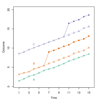
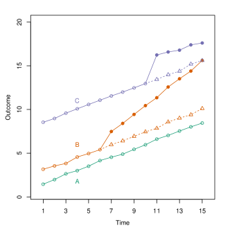
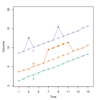
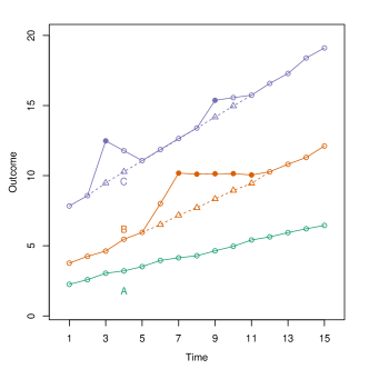
Note: The above figures show outcome trajectories of units in a staggered adoption setting (a) and in a general setting (b). Solid and hollow circles represent observed outcomes under the treatment and control conditions, respectively, while triangles represent counterfactual outcomes (in the absence of the treatment). The data on the left panels in both (a) and (b) are generated by DGPs that satisfy TWFE assumptions while the data on the right are not. The divergence between hollow circles and triangles in the right panel of (b), both of which are under the control condition, is caused by carryover effects.

A third limitation of the canonical TWFE model is its presumption of no temporal and spatial interference. In most uses of TWFE models, researchers assume that there are no spatial spillovers and that treatment effects occur contemporaneously, hence no anticipation or carryover effects. These are obviously strong assumptions that are rarely questioned or tested in practice (Imai and Kim, 2019; Athey and Imbens, 2022; Wang, 2021). Although some recent methods permit arbitrary carryover effects in staggered adoption settings (Strezhnev, 2018; Callaway and Sant’Anna, 2021), they are not distinguishable from contemporaneous effects. This limitation becomes more complex when treatment reversal is possible, as demonstrated in Figure 1. In Figure 1(b), data in the left panel are consistent with TWFE assumptions, while the right panel shows deviations from the PTA, constant treatment effect, and the absence of anticipation or carryover effects. What is concerning is that many real-world data resemble the problematic right figure rather than the ideal left one. Nevertheless, recent methods have been proposed to handle arbitrary carryover effects over a limited number of periods in more general settings (IKW 2023; LWX 2022). The challenge of addressing spatial spillover effects without strong structural assumptions still persists (Aronow, Samii and Wang, 2020; Wang, 2021), but its resolution is beyond the scope of this paper.

Notation and Causal Estimands.

Consider the panel setting where multiple units $i\in\{1,\dots,N\}$ are observed at each time period $t\in\{1,\dots,T\}$. Each unit-time pair $(i,t)$ uniquely identifies an observation. For each $i$, let $E_{i,t}=\max\{t^{\prime}:t^{\prime}\leq t,D_{i,t^{\prime}}=1,D_{i,t^{\prime}-1}=0\}$ for all $t$ such that $\exists s\leq t:D_{i,s}=1$ and $E_{i,t}=\min\{t^{\prime}:D_{i,t^{\prime}}=1,D_{i,t^{\prime}-1}=0\}$ otherwise. That is to say, $E_{i,t}$ is the most recent time at which unit $i$ switched into treatment or, if $i$ has not yet been treated at any point up until time $t$, the first time $i$ switches into treatment. If $i$ is never treated, we let $E_{i,t}=\infty$. In the staggered setting, we call this the “event time” $E_{i}=E_{i,t}$, and $D_{i,t}=\mathbf{1}\left\{t\geq E_{i,t}\right\}$, where $\mathbf{1}\left\{\cdot\right\}$ is the indicator function. In a staggered adoption context, we partition units into distinct “cohorts” $g\in{1,\dots,G}$ according to the timing of treatment adoption $E_{i,t}$. Units transitioning to treatment at period $g$ ($i$ such that $E_{i,t}=g$) form cohort $g$, whereas units that never undergo treatment belong to the “never-treated” cohort ($i:E_{i,t}=\infty$). $Z_{i,t}$ ($Z_{i,g,t}$) represents the variable $Z$ for unit $i$ (part of cohort $g$) at time $t$. We use $Y_{i,t}(1)$ and $Y_{i,t}(0)$ to denote the potential outcomes under treatment and control, respectively, and $Y_{i,t}=D_{i,t}Y_{i,t}(1)+(1-D_{i,t})Y_{i,t}(0)$ to denote the observed outcome.

The finest estimand is the ITE, $\tau_{i,t}=Y_{i,t}(1)-Y_{i,t}(0)$, of which there exists one for each observation $(i,t)$. Most political science research, however, typically focuses on estimating a single summary statistic. Commonly, this is the ATT, which represents ITE averaged over all observations exposed to the treatment condition. In between these extremes of granularity and coarseness are time-varying dynamic treatment effects (DTE), which are across-unit averages of ITE at each time period relative to treatment adoption (e.g., all observations immediately proceeding treatment adoption). In the staggered adoption setting, we can further subdivide by cohort. We denote the DTE $l$ periods after treatment adoption (for treatment cohort $g$) as $\delta_{l}$ ($\delta_{g,l}$) and use $l=1$ to represent the period immediately after treatment adoption. $\delta_{g,l}$ is also what some authors refer to as cohort average treatment effect on the treated (CATT) (Strezhnev, 2018; Sun and Abraham, 2021) or group-time average treatment effect (Callaway and Sant’Anna, 2021).

Each of the estimators we discuss can be used to estimate $\delta_{l}$. The analogous specification for estimating DTE is a lags-and-leads specification. Let $K_{i,t}=(t-E_{i,t}+1)$ be the number of periods since the most recent event date that unit $i$ has been in treatment at period $t$ ($K_{i,t}=1$ if unit $i$ switches into treatment at time $t$). Consider a regression based on the following specification:

$$Y_{i,t}=\alpha_{i}+\xi_{t}+X^{\prime}_{i,t}\beta+\sum_{\begin{subarray}{c}l=-a\\ l\neq 0\end{subarray}}^{b}\delta_{l}^{TWFE}\cdot\mathbf{1}\left\{K_{i,t}=l\right\}+\delta_{b+}^{TWFE}\mathbf{1}\left\{K_{i,t}>b\right\}\cdot D_{i,t}+\varepsilon_{i,t},\vspace{-1em}$$ (3)

where $a$ and $b$ are the number of lag and lead terms (BJS 2023). In the social science literature, the typical practice is to exclude $l=0$, which corresponds to the time period immediately before the transition into the treatment phase, and use it as a reference period as suggested by Roth (2022). Conventionally, $\hat{\delta}^{TWFE}_{l}$ is interpreted as an estimate of $\delta_{l}$ or as a meaningful weighted average of pertinent ITE. Meanwhile, $\hat{\delta}^{TWFE}_{b+}$ is viewed as an estimate for the long-term effect. We refer readers to the section on “Implementation Details” in the SM for more information on Model (3), including in the case where there are treatment reversals.

3.  HTE-Robust Estimators

In this section, we offer a brief overview and comparison of several recently introduced HTE-robust estimators. For a more comprehensive discussion, please refer to the SM.

Summary of HTE-robust estimators.

Table 1 summarizes the estimators we discuss in this paper. The primary difference resides in the mechanics of their estimation strategies: there are methods based on canonical DIDs and methods based on imputation. We refer to the former as DID extensions and the latter as imputation methods. DID extensions use DTE, estimated from local, $2\times 2$ DIDs between treated and control observations, as building blocks. Imputation methods use ITE, estimated as the difference between an imputed outcome under control and the observed outcome (under treatment), as building blocks. Imputation methods connect to TWFE through the outcome model, which is fit globally on all available controls, that they use to impute counterfactual outcomes. Different strategies also entail different assumptions. Each DID extension, for example, relies on a particular type of PTA, whereas imputation methods presuppose a TWFE model for untreated potential outcomes and require a zero mean for the error terms.

Another noteworthy difference lies in the settings in which these estimators are applicable: some function exclusively in settings with staggered treatment adoption, while others can accommodate scenarios with treatment reversals. Furthermore, these estimators diverge in terms of (1) how they select untreated observations as controls for treated units, (2) how they incorporate pre-treatment or exogenous covariates, and (3) the choice of the reference period. We discuss these details further below and in the ‘Survey of HTE-Robust Estimators’ and ‘Implementation Details’ sections of the SM.

Table 1: Summary of HTE-Robust Estimators

Type	DID Extensions: uses $2\times 2$ DIDs as building blocks				Imputation Methods
Setting	Staggered: treatment reversals not allowed		General: treatment reversals allowed
Research article	Sun and Abraham (2021)	Callaway and Sant’Anna (2021)	de Chaisemartin and D’Haultfœuille (2020)	IKW (2023)	BJS (2023)	LWX (2022)
Method known as	interaction weighted	csdid	did_mulitple	PanelMatch	DIDM	FEct
Key ID assumption	Parallel trends	Parallel trends	Parallel trends	Parallel trends	Zero conditional mean	Strict exogeneity
Finest estimand	$\delta_{g,l}$	$\delta_{g,l}$	$\delta_{l}$	$\delta_{l}$	$\tau_{i,t}$	$\tau_{i,t}$
Comparison group	Never-treated or last-treated	Never-treated or not-yet-treated	Matched stable group (not-yet-treated)	Matched stable group (not-yet-treated)	Imputed Counterfactual (not-yet-treated)	Imputed Counterfactual (not-yet-treated)
Reference period(s)	Period 0	An arbitrary pre-treatment period	Untreated period	Period 0	All pre-treatment periods	All pre-treatment periods
Covariate adjustment	Possible extension	Outcome & propensity score modeling	Possible extension	Refined matched set & outcome modeling	Outcome modeling	Outcome modeling

DID extensions.

DID extensions are all built from local, $2\times 2$ DID estimates—hence our choice of terminology. The overarching strategy for these estimators is to estimate the DTE, $\delta_{l}$ (or $\delta_{g,l}$ for each cohort $g$ in the staggered setting), for each period since the most recent initiation of treatment, $l$, using one or more valid $2\times 2$ DIDs. By ‘valid,’ we mean that the DID includes (1) a pre-period and a post-period and (2) a treated group and a comparison group. The pre-period is such that all observations in both groups are in control, while the post-period is such that observations from the treated group are in treatment and those from the comparison group are in control. The choice of the comparison group is the primary distinction between estimators in this category. To obtain higher-level averages such as the ATT, we then average over our estimates of $\delta_{l}$ (or $\delta_{g,l}$), typically employing appropriate, convex weights.

We cover two estimators in this category that are appropriate only for the staggered setting. Sun and Abraham (2021) propose an interaction-weighted (iw) estimator, which is a weighted average of $\delta_{g,l}$ estimates obtained from a TWFE regression with cohort dummies fully interacted with indicators of relative time to the onset of treatment. They demonstrate that each resulting estimate of $\delta_{g,l}$ can be characterized as a difference in the change in average outcome from a fixed pre-period $s<g$ to a post-period $l$ periods since $g$ between the treated cohort $g$ and the comparison cohorts in some set $\mathcal{C}$. The authors recommend using $\mathcal{C}={\sup_{i}E_{i}}$, which is either the never-treated cohort or, if no such cohort exists, the last-treated cohort. By default, iw uses $l=0$ as the reference period and can accommodate covariates in the TWFE regression.

Employing the same general approach, Callaway and Sant’Anna (2021) propose two estimators, one of which uses never-treated units ($\hat{\delta}^{CS-dr}_{nev}$) and the other not-yet-treated units ($\hat{\delta}^{CS-dr}_{ny}$) as the comparison group. We label these estimators collectively as csdid. Note that $\hat{\delta}^{CS-dr}_{nev}$ uses the same comparison group as iw when a never-treated cohort exists, whereas $\hat{\delta}^{CS-dr}_{ny}$ uses all untreated observations of not only never-treated units but also later adopters as controls for earlier adopters. Besides the choice of comparison cohort, csdid estimators differ from iw in that they allow users to condition on pre-treatment covariates using both an explicit outcome model and inverse probability weighting (IPW) simultaneously, with at least one needing to be correct for the estimator to be consistent. We will only implement $\hat{\delta}^{CS-dr}_{ny}$, as most models in our replication sample do not include additional covariates, rendering $\hat{\delta}^{CS-dr}_{nev}$ and $\hat{\delta}^{IW}$ numerically identical. While iw uses one period before the treatment’s onset as the reference period, csdid allows users to choose one or multiple pre-treatment periods as the reference

In settings with treatment reversals, separate groups of researchers have converged on the same strategy for choosing a comparison group: matching treated and control observations that belong to units with identical treatment histories. IKW (2023) suggest one such estimator, PanelMatch, which begins by constructing a “matched set” for each pair $(i,t)$ such that unit $i$ transitions into treatment at time $t$. This matched set includes units that are both (1) not under treatment at time $t$ and (2) share the same treatment history as $i$ for a fixed number of periods leading up to the treatment onset. For each post-period $l$ periods since treatment adoption, it then estimates a local DID. It uses a fixed pre-period $s<t$ and the post-period $t-1+l$. The treatment “group” comprises solely of $(i,t)$, and the members of the matched set for $(i,t)$ that are still under control during the post-period serves as the comparison group. To obtain $\delta_{l}$ for a given $l$, it then averages over the local estimates from all treated $(i,t)$ such that $(i,t+l-1)$ is still under treatment (i.e., no treatment reversal has occurred yet). IKW (2023) propose incorporating covariates by “refining” matched sets and use $l=0$ as the reference period.

Using a similar strategy, de Chaisemartin and D’Haultfœuille (2020) propose a “multiple DID” estimator, DID_M. Importantly, they include local DIDs for units leaving treatment and not only those joining treatment. DID_M also only consider the case where we match on a single period and where $l=1$. Consequently, their target estimand is not the ATT but rather an average of the contemporaneous effects of “switching” (i.e., the effect of joining or the negative of the effect of leaving at the time of doing so). Interestingly, another DID extension can be seen as a special case of PanelMatch: In the staggered setting, the PanelMatch estimator aligns with the not-yet-treated version of csdid (without covariate adjustment). We delve into details on the connections between these three estimators in the ‘Survey of HTE-Robust Estimators’ section of the SM.

All DID extensions are built using local, $2\times 2$ DIDs, and their assumptions reflect this. Specifically, they each rely on a form of the PTA—that is, the expected changes in potential outcomes under control from one period to the next are equal between the treated and the chosen comparison groups. In Table 1, we refer to all these assumptions collectively as the PTA. We defer readers to the SM for a fuller account of each method’s assumptions.

The imputation method.

Imputation estimators do not explicitly estimate local DIDs. Instead, they take the difference between the observed outcome and an imputed counterfactual outcome for each treated observation. The connection to the TWFE model is in the functional form assumption used to impute counterfactual outcomes. Specifically, an imputation estimator first fits a parametric model for the potential outcome under control $Y_{i,t}(0)$—in our case, this is Model (1)—using only control observations $\{(i,t):D_{i,t}=0\}$. It is also through this outcome model that one can adjust for covariates. Then, it imputes $Y_{i,t}(0)$ for all treated observations $\{(i,t):D_{i,t}=1\}$ using the estimated parameters. Finally, it estimates the ITE, $\tau_{i,t}$, for each treated observation $(i,t)$ by calculating the difference between its observed outcome $Y_{i,t}=Y_{i,t}(1)$ and its imputed counterfactual outcome $\hat{Y}_{i,t}(0)$. Inference for the estimated $\hat{\tau}_{i,t}$ is possible, although uncertainty estimates need to be adjusted to account for the presence of idiosyncratic errors (e.g., Bai and Ng, 2021). BJS (2023) and LWX (2022) each propose estimators in this category. Each group proposes a more general framework that nests many models, including TWFE. The latter also introduces several specific imputation estimators. One of these uses the TWFE model, and the authors refer to the resulting astimator as the fixed effect counterfactual estimator, or FEct.

Compared to DID extensions, which typically use a single pre-period and, with the exception of csdid, only a subset of units under control at both the pre- and post-periods as a comparison group, imputation estimators use all available control observations to estimate treated counterfactuals. As such, for each unit, the reference period can be understood as (the average of) all pre-treatment periods. Intuitively, this approach should result in higher efficiency. In fact, BJS (2023) demonstrate that imputation estimators are the most efficient among all estimators under the condition of homoskedastic errors. Also in contrast to DID extensions, imputation estimators do not directly assume the PTA. Instead, they restrict the expectation of the error terms from a parametric TWFE model. In Table 2, this is denoted as “zero conditional mean” for BSJ (2023) or “strict exogeneity” for LWX (2022). Again, we refer readers to the SM for the formal statements of these assumptions. Collectively, these assumptions imply a form of conditional, baseline randomization of treatment assignment, which in turn implies the PTA (e.g., Blackwell and Glynn, 2018).

Although DID extensions and imputation methods rely on slightly different identification assumptions, such as the PTA and specific constraints on the error terms, they usually lead to similar observable implications. Researchers commonly use the presence or absence of pretrends in the pre-treatment periods to judge the plausibility of the PTA. In the classic two-group, two-period setting, if there are data from additional pre-treatment periods, researchers can plot the time series of (average) outcomes of each group and visually inspect whether they indeed trend together. The intuition is that if the PTA holds and the outcome trends of the treated and control groups are indeed parallel when $Y(0)$’s are observed for all units, then it is plausible that the PTA also holds in the post-treatment periods, when $Y(0)$’s are no longer observable for units in the treatment group. Conversely, differential trends in the pre-treatment periods should make us suspicious of the PTA. In more complex settings or where we wish to control for observed confounders, we can substitute the outcome time series with estimates of the dynamic effects before the onset of treatment, $\delta_{l}$ for $l\leq 0$. If the PTA holds, then these pre-treatment effect estimates should be zero. We provide a more thorough discussion and examples of DTE plots, which are also known as “event study plots,” in the next section when we introduce our procedure.

4.  Data and Procedure

Next, we assess the robustness of empirical findings from causal panel analyses in political science and compare results obtained using the different methods we have discussed. We will explain our sample selection rules, describe standard practices in the field, and outline our reanalysis approach. Readers can find a more detailed explanation of our sample selection criteria and replication and reanalysis procedure in the “Sample and Replicability” and “Implementation Details” sections of the SM.

Data.

Our replication sample comprises articles from three leading political science journals—the APSR, AJPS, and JOP—published over a recent six-year span from 2017 to 2022. We initially include all studies, including both long and short articles, that employ panel data analyses with a binary treatment as a crucial component of their causal argument, resulting in a total of 90 articles. After a careful review of each of these articles, we find that 52 articles use a TWFE model similar to Model (1). We then attempt to replicate the main results of these 52 articles and are successful in 37 cases (71.2%). A detailed explanation of how we select the “main model” is provided in the ‘Sample and Replicability’ section of the SM. Table 2 depicts the distribution of successful replications, along with reasons for replication failures, across the various journals.

Table 2: Sample Selection and Replicability of Qualified Articles

		TWFE	Incomplete	Replication		Success
Journal	All	(attempted)	data	error	Replicable	Rate%
APSR	18	9	2	1	6	66.7
AJPS	28	18	3	3	12	66.7
JOP	44	25	6	0	19	76.0
Total	90	52	11	4	37	71.2

Settings and common practices.

Table 3 presents an overview of the standard practices and settings in the articles that we successfully replicated. The vast majority of studies in our sample (92%) use DID designs to justify the use of the TWFE model, while the remaining studies advocate for the model’s ability to exploit “within” variations in the data. Out of the 37 articles, five (13%) employ a classic DID design, which includes two-group, two-period designs (three articles) and multi-period DID designs (two articles). 10 articles (27%) use a staggered (but not classic) DID design, while the remaining 22 articles (59.5%) fall into the “general” category, meaning they allow for treatment reversals. Except for four articles, all studies have a continuous outcome of interest. Most studies adopt cluster-robust SEs or panel-corrected SEs (Beck and Katz, 1995), while five articles apply bootstrap procedures for estimating uncertainties. A subset of authors explore alternative model specifications by adding LDVs (six articles), ULTs (11 articles) and higher-than-unit-level time trends (5 articles). Notably, 22 studies use some type of plot—either average outcomes over time, DTE/event-study plots, or both—to evaluate the plausibility of the PTA.

Table 3: Settings and Common Practice

Motivations for TWFE				Variance Estimator
“Difference-in-differences”	34	92%		Cluster-robust SE or PCSE	36	97.3%
“Within” variations	3	8%		Cluster-bootstrapped procedures	5	13.5%
Treatment Setting				Variants in specifications
Classic 2$\times$2 DID	3	8.1%		LDVs	6	16.2%
Classic multi-period DID	2	5.4%		Higher-than-unit-level time trends	5	13.5%
Staggered DID	10	27%		ULTs	11	29.7%
General	22	59.5%
				Data visualization
Outcome Variable				Group average outcomes	14	37.8%
Continuous	33	89.2%		DTE/event-study plots	18	48.6%
Binary	4	11.8%		Neither	15	40.5%

Procedure.

We use data from Grumbach and Sahn (2020) to illustrate our process for replication and reanalysis. The study investigates the influence of coethnic mobilization by minority candidates during US congressional elections. To simplify our analysis, we focus on the impact of the presence of an Asian candidate on the proportion of general election contributions from Asian donors.

To begin, we aim to understand the research setting and data structure. We visualize the patterns of treatment and outcome variables using plots like Figure 3 (a) and (b). In this application, treatment reversals clearly take place. Some data is missing (due to redistricting), but the issue does not seem to be severe. We record important details such as the number of observations, units, and time periods, the type of variance estimators, and other specifics of the main model (not shown here). Next, we replicate the main finding, employing both the original variance estimator and a cluster-bootstrap procedure. We also use a bootstrap refinement procedure recommended by Cameron, Gelbach and Miller (2008) to conduct statistical testing; the results are broadly consistent with the ones based on cluster-bootstrapped SEs and CIs.

Figure 2: Visualizing Data from Grumbach and Sahn (2020)

(a) Treatment Status

(b) Outcome Variable

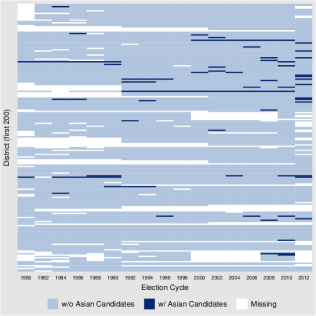
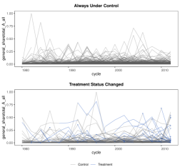
Note: Visualizing data from Grumbach and Sahn (2020), who investigate the effects of Asian candidates in congressional elections on the share of campaign contributions by Asian donors.

We then re-estimate the ATT and DTEs using estimators discussed in Section 3. For staggered adoption treatment cases, we apply six estimators: TWFE (with always treated units removed for easier comparisons with other estimators), PanelMatch, FEct, Stacked DID, iw, and csdid (not-yet-treated). For applications with treatment reversals like Grumbach and Sahn (2020), we use the first three estimators only. The comparison between the TWFE estimate and the other estimates sheds light on whether original findings are sensitive to the presence of HTE. Results from this example are shown in Figures 3(a)-(d). The similarity between estimates for ATTs in (a) suggests the robustness of the original finding to the choice of estimators. The DTE plots from HTE-robust estimators in (c)-(d) are broadly consistent with the DTE plot from TWFE in (b).

Figure 3: Reanalysis of Grumbach and Sahn (2020)

(a) Treatment effect estimates

(b) DTE: TWFE

(c) DTE: PanelMatch

(d) DTE: FEct

(e) Placebo test

(f) Test for carryover effects

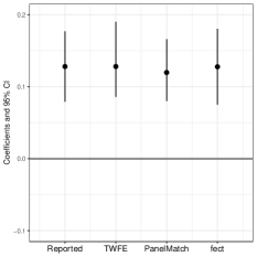
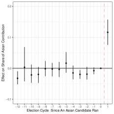
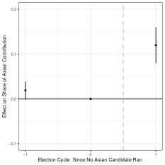
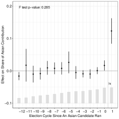
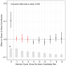
Note: Reanalysis of data from Grumbach and Sahn (2020). Subfigures (a): Treatment effect or ATT estimates from multiple methods; subfigures (b)-(d): DTE plots using TWFE, PanelMatch, and FEct; Subfigure (e)-(f): results from the placebo test and test for carryover effects usingFEct—the blue points in (g) and red points in (h) represent the holdout periods in the respective tests. CIs for TWFE, PanelMatch, and FEct In all subfigures are produced by bootstrap percentile methods.

Finally, we conduct diagnostic tests based on FEct to further assess the PTA and, in applications with treatment reversal, the no-carryover-effect assumption. We use FEct because it is applicable across all studies in our replication sample and does not discard data. One important caveat is that the results of these formal statistical tests need to be combined with visual inspections of DTE plots, as they may either suffer from low power with a small sample size or be “too powerful” with abundant data. To guard against the latter possibility, we also perform an equivalence test of the null that pre-treatment (or carryover) effects are “large,” i.e. outside of some $\theta$-neighborhood of 0. Note this test requires us to specify a threshold $\theta$, and we conduct tests with a default threshold and with the ATT set as the threshold. Small $p$-values are evidence in favor of the claim that PTA violations are either nonexistent or mild. Figures 3(d), (e) and (f) show the results from the $F$ test, placebo test, and test for no carryover effects on our running example, respectively. Both a visual inspection and the formal tests suggest that the PTA and the no-carryover-effect assumption are quite plausible.

On the whole, the result from Grumbach and Sahn (2020) that we reanalyze seems highly robust. The study also seems to have sufficient power to not only distinguish the ATT from zero, but also to assess the validity of its identification assumptions. There is strong evidence that the PTA is satisfied and that there are no carryover effects. The results are consistent across choice of estimator and robust to using cluster-bootstrapped standard errors.

5.  Systematic Assessment

We carry out the replication and reanalysis procedure described above for all 37 articles in our sample. This section offers a summary of our findings; the complete results for each paper can be found in the SM. We structure our results around two main questions: (1) Is the PTA plausible, and (2) do HTE-robust estimators provide results that are qualitatively different from those obtained with TWFE? Additionally, we report on other issues we observe in the replicated articles, which include lack of statistical power, presence of carryover effects, and lack of robustness to alternative specifications, such as the addition of LDVs or ULTs.

PTA violations remain a concern.

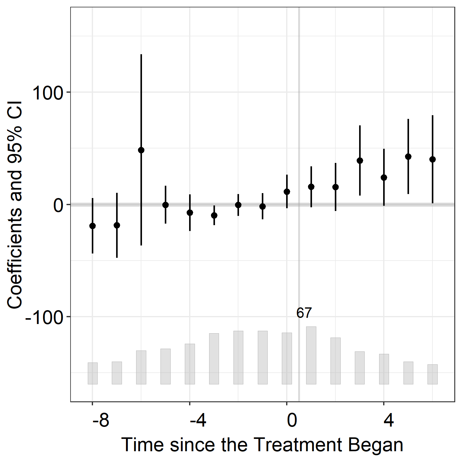
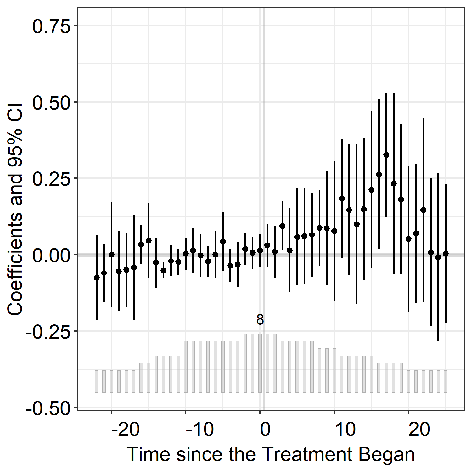
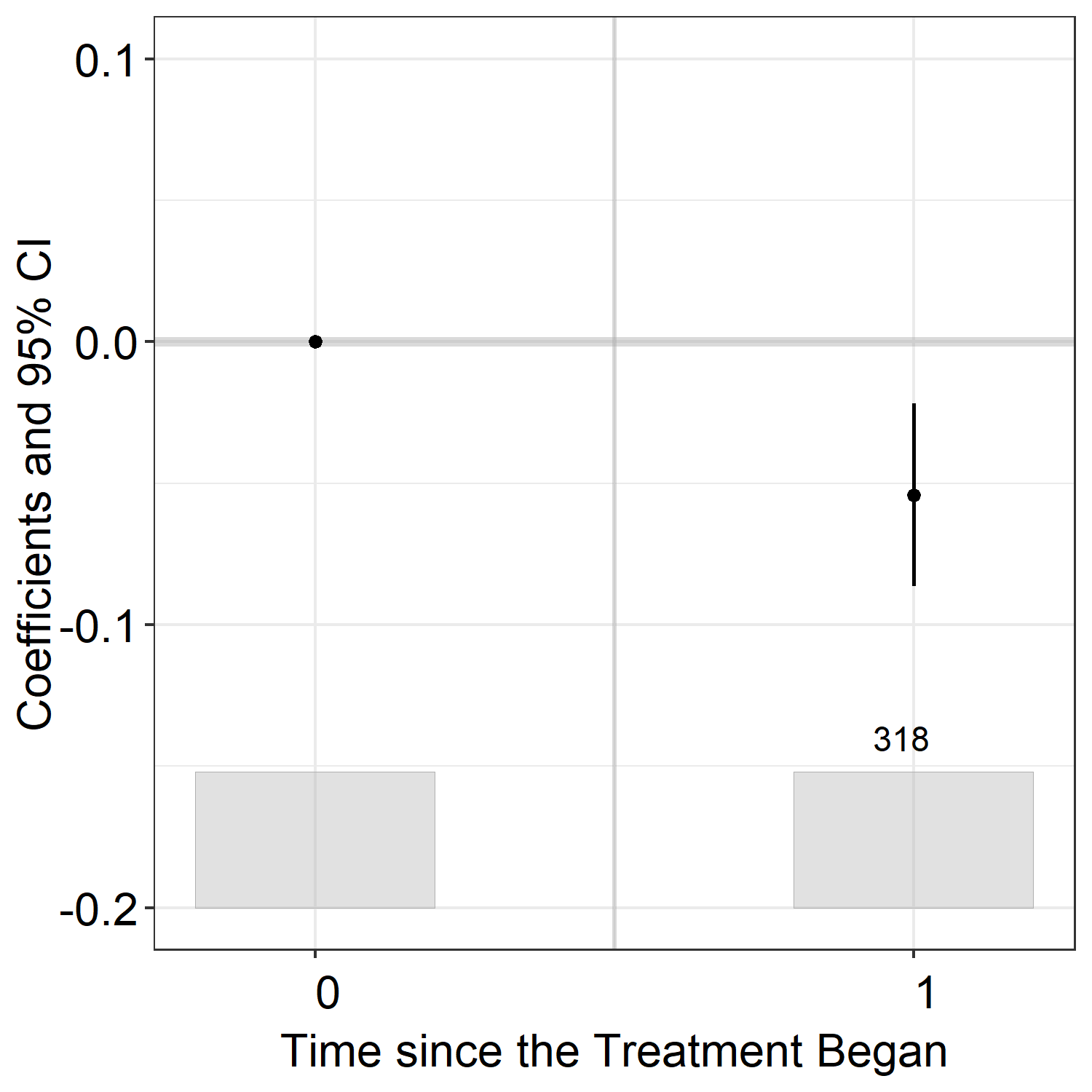
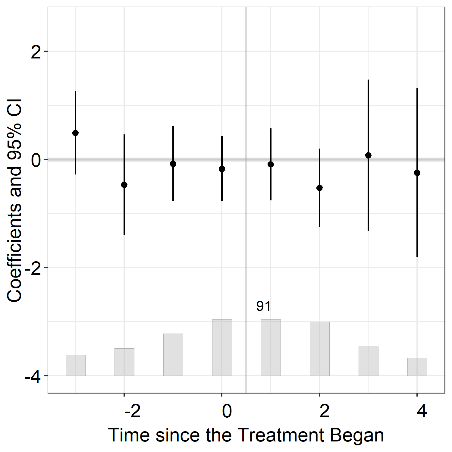
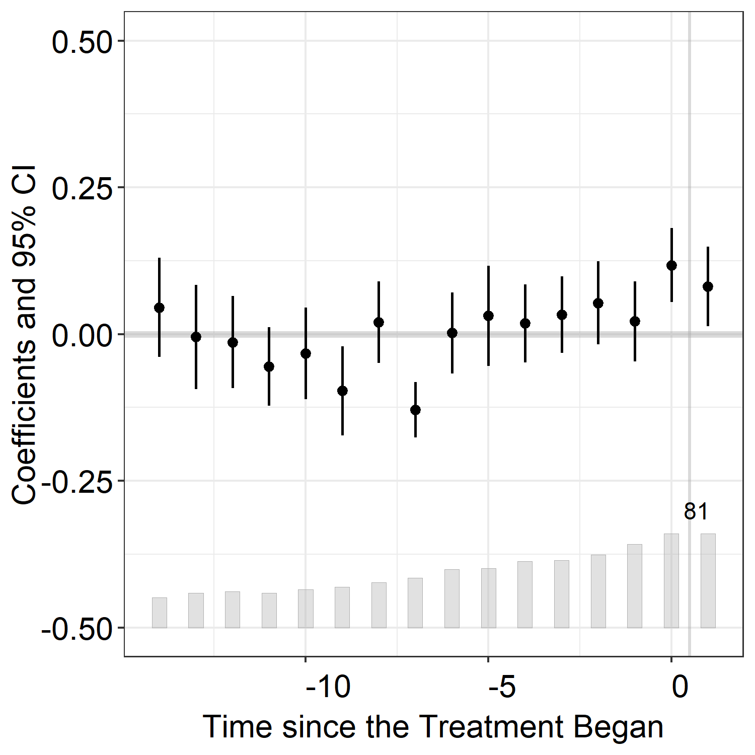
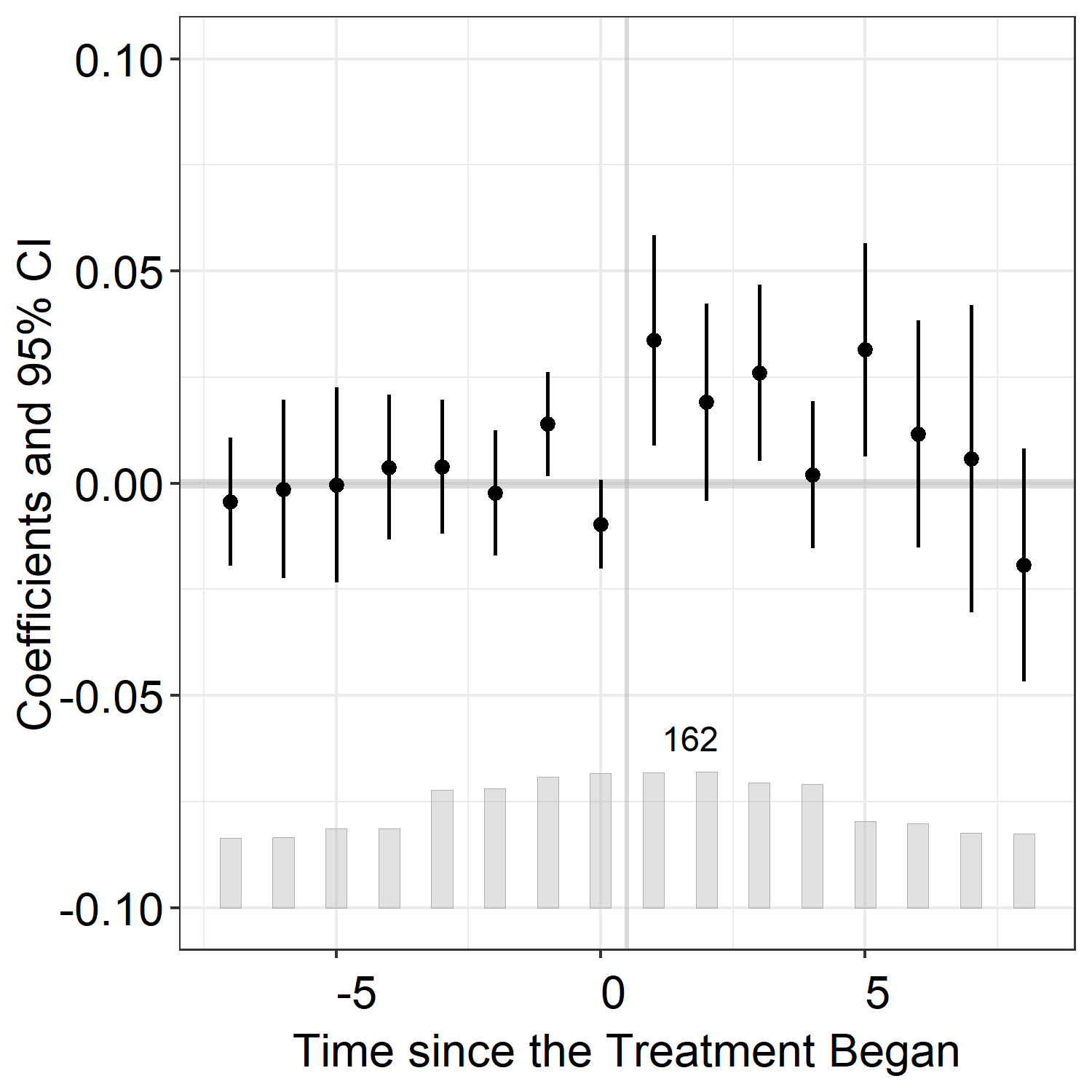
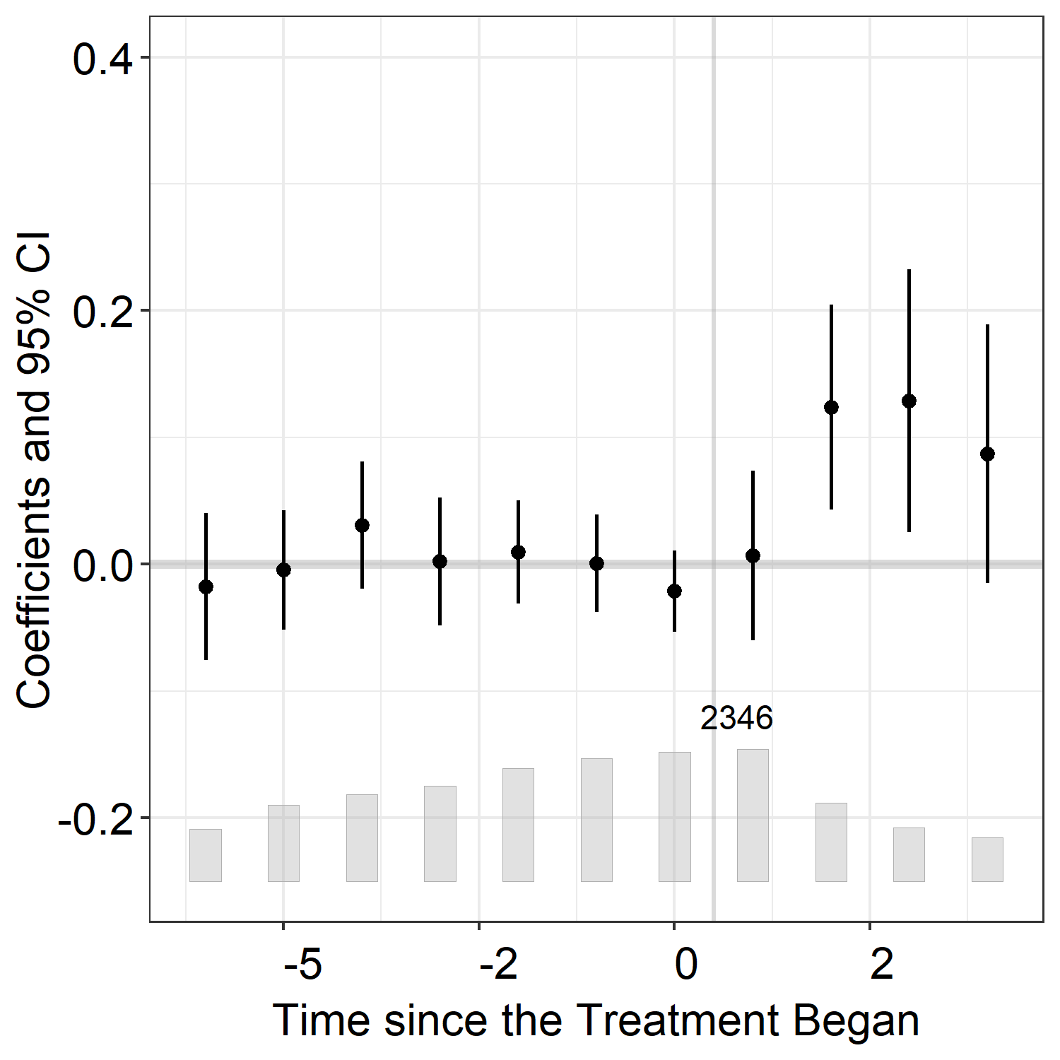
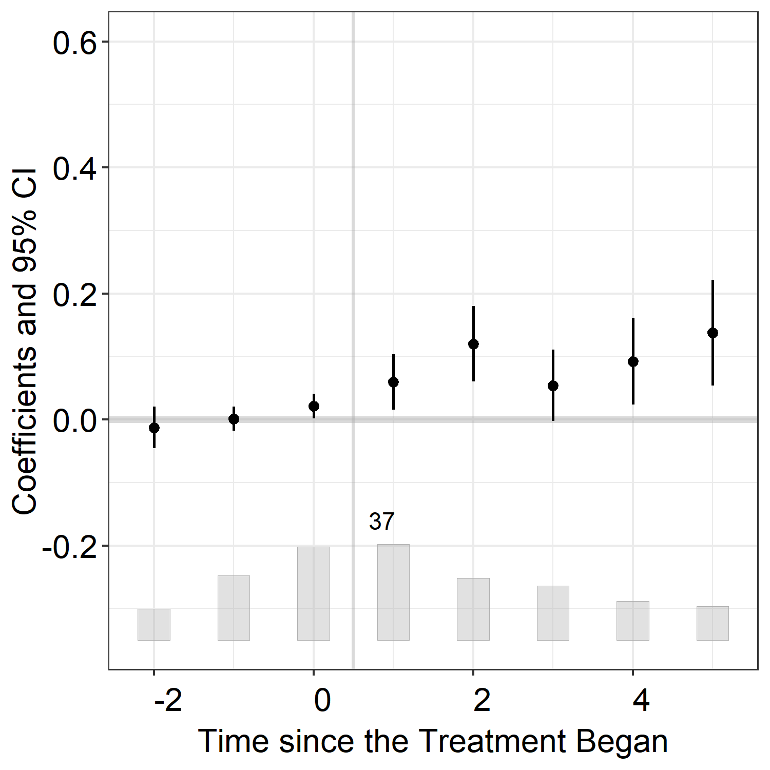
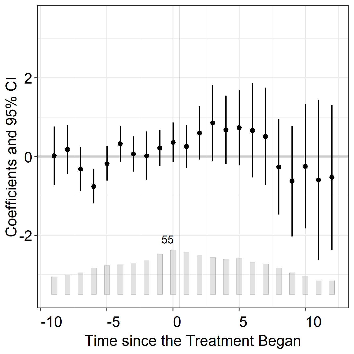
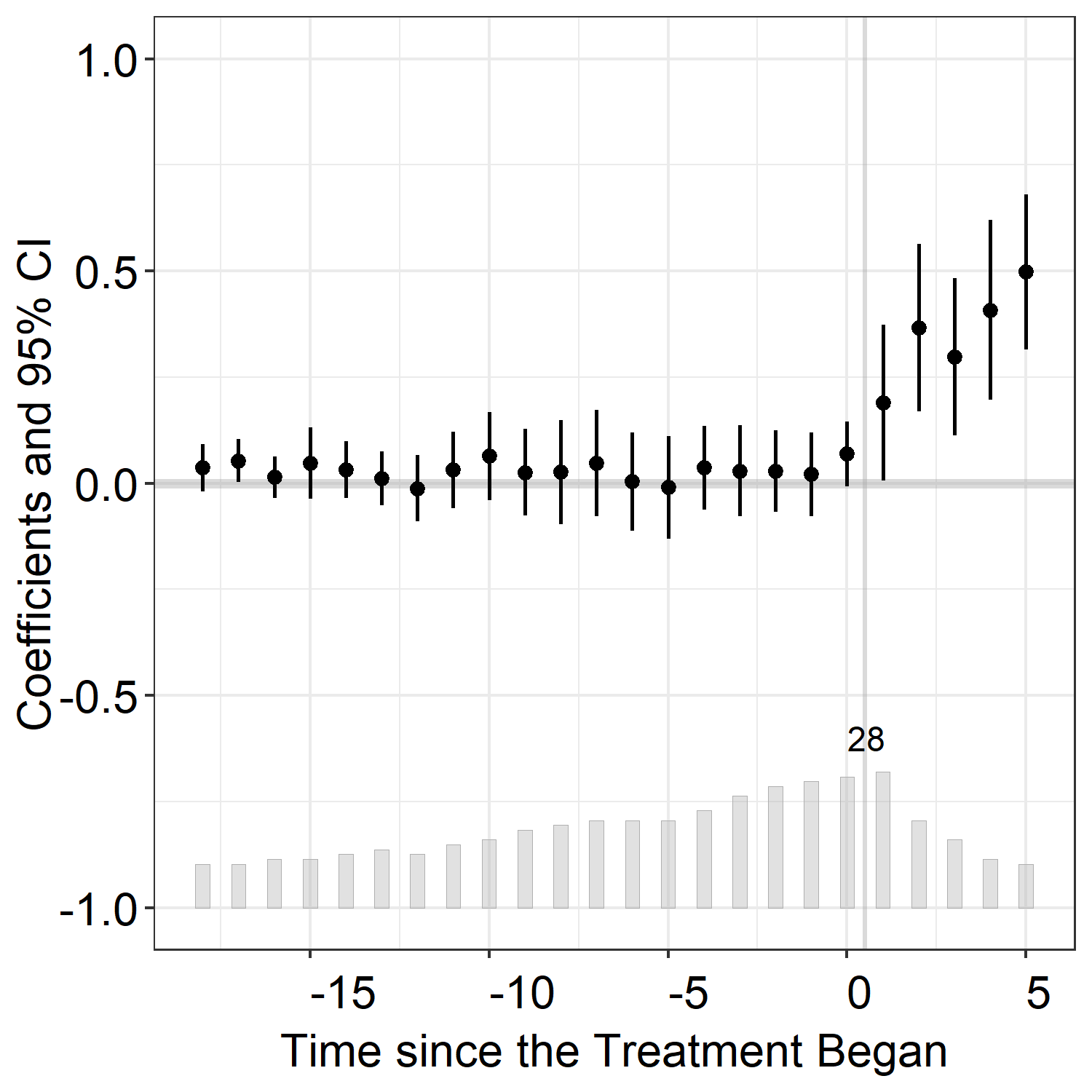
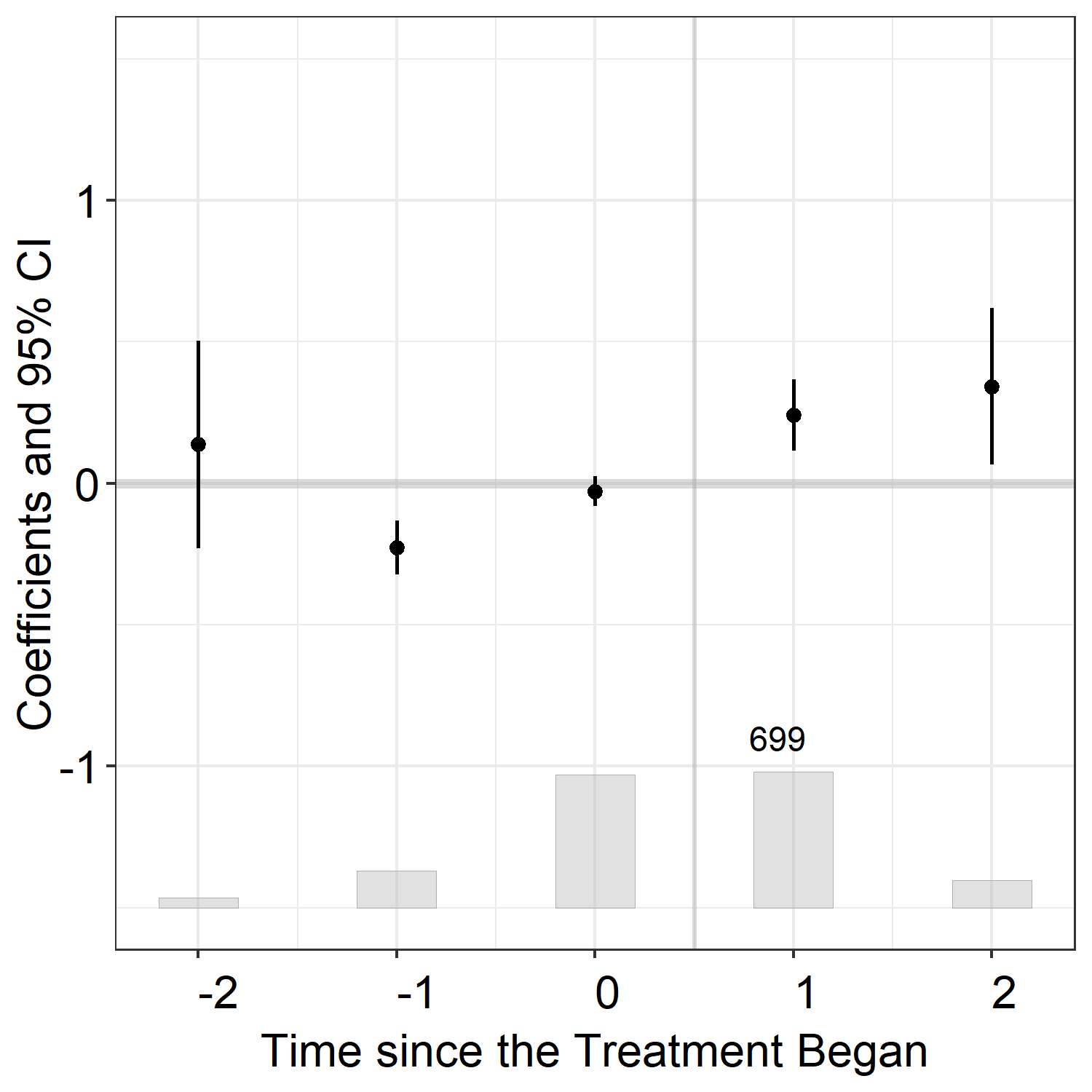
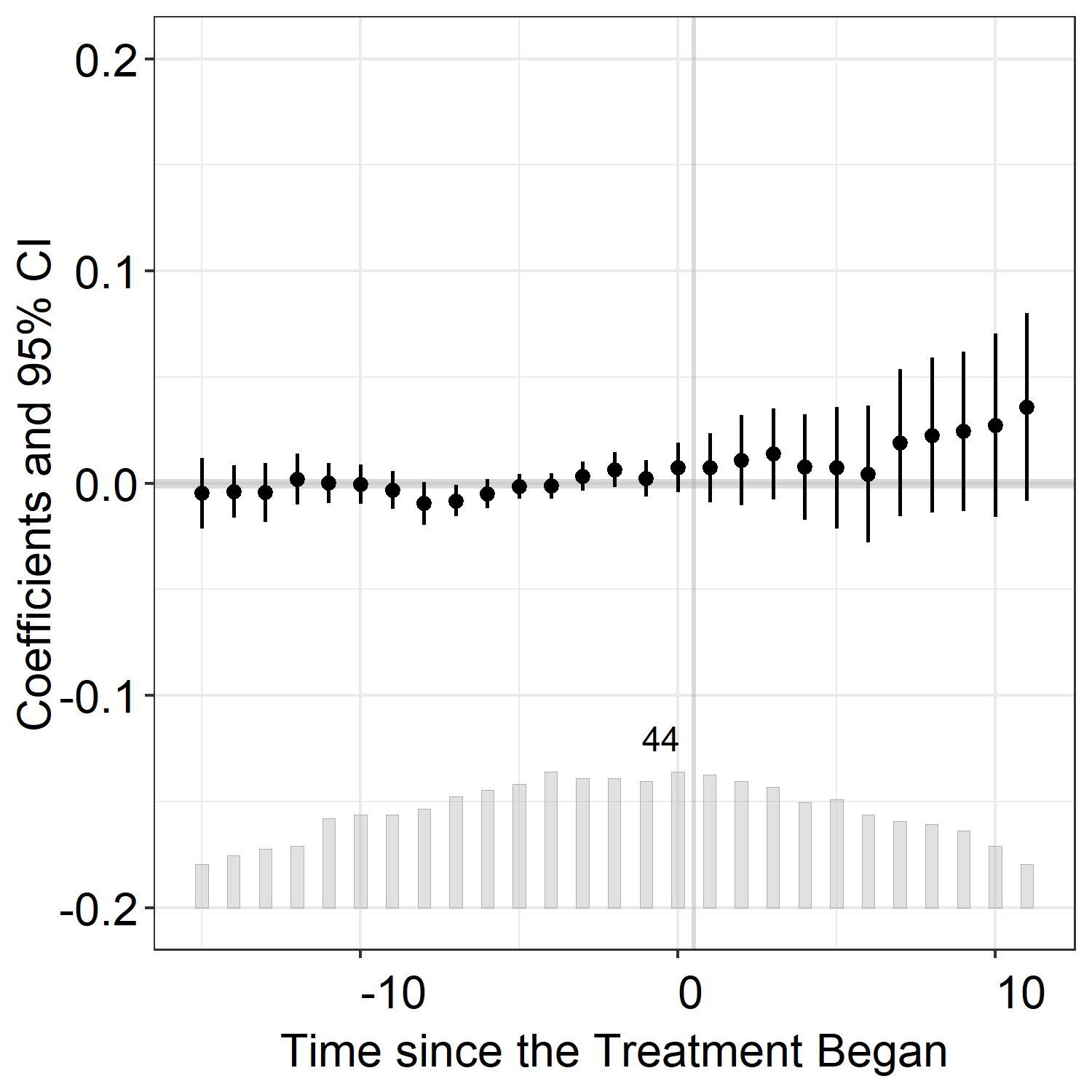
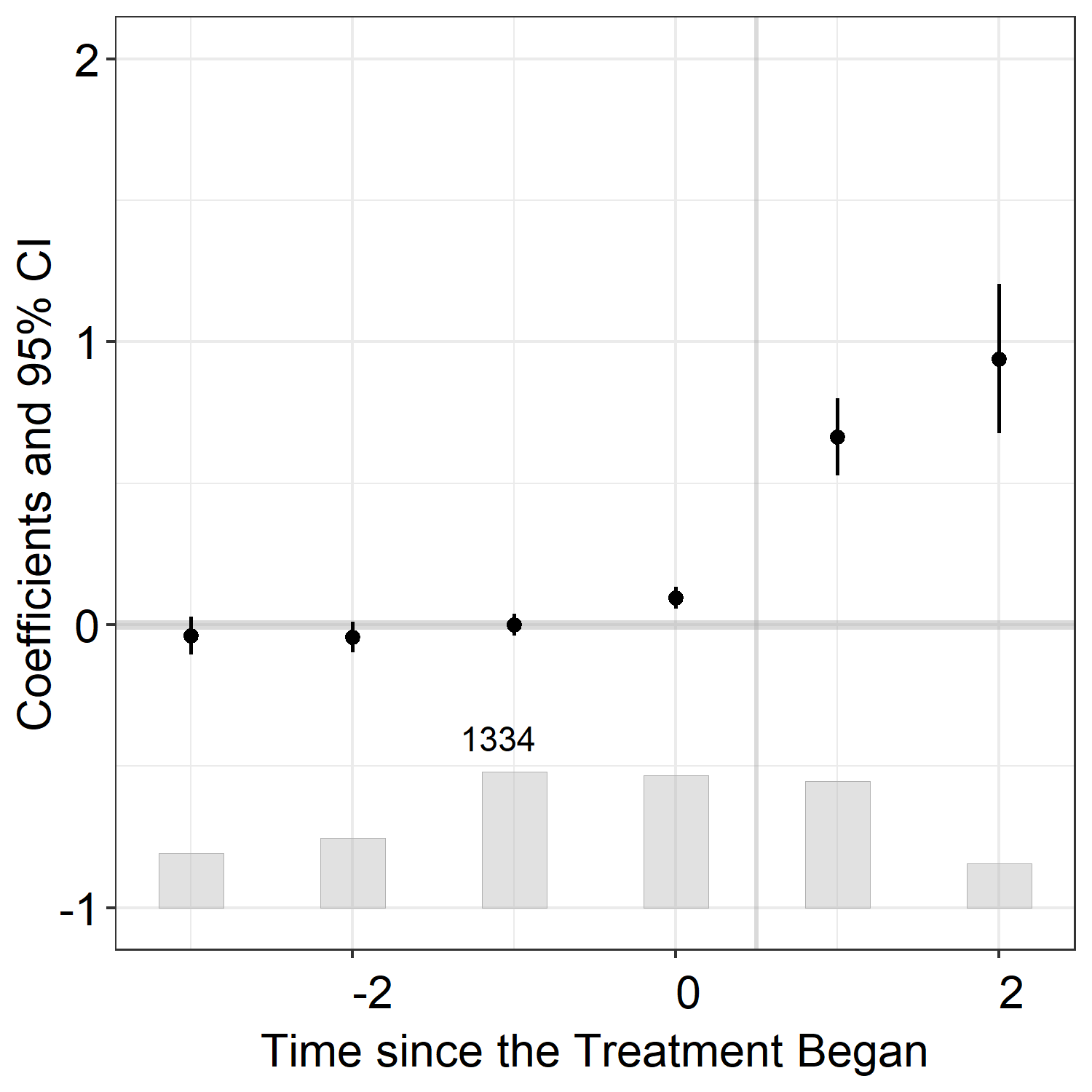
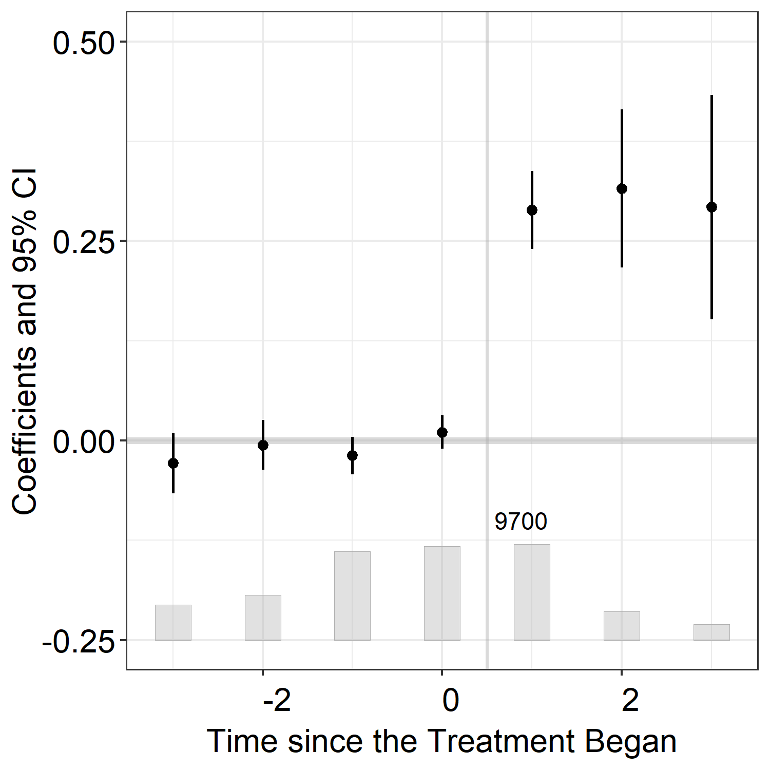
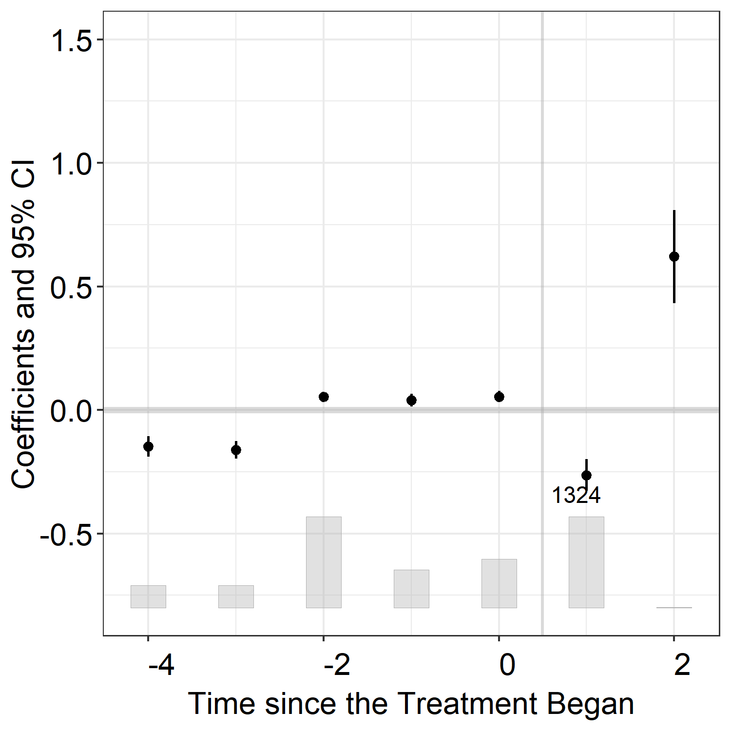
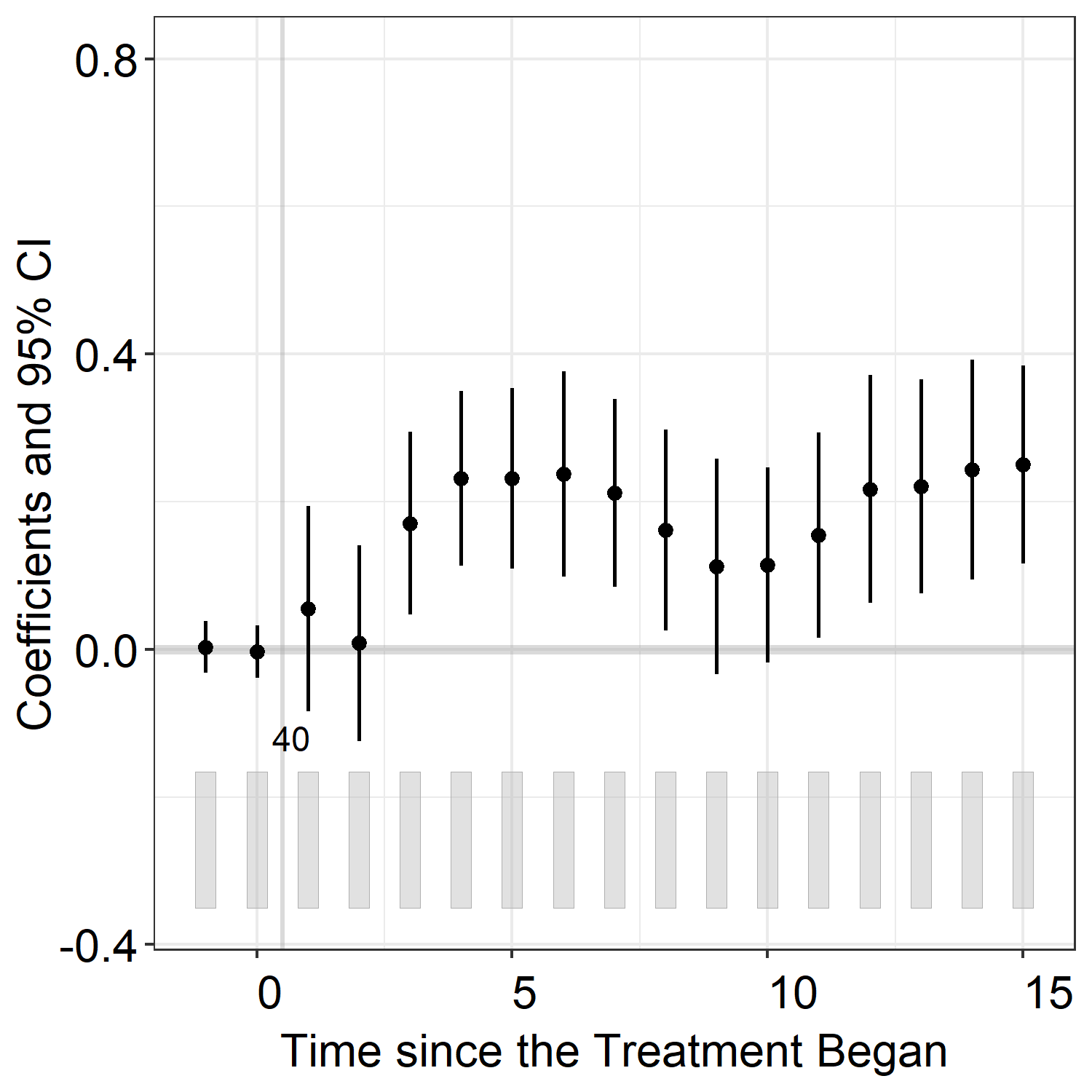
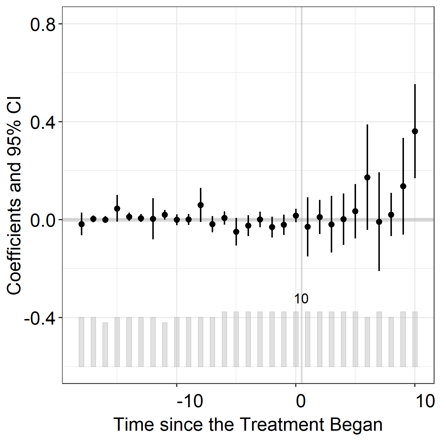
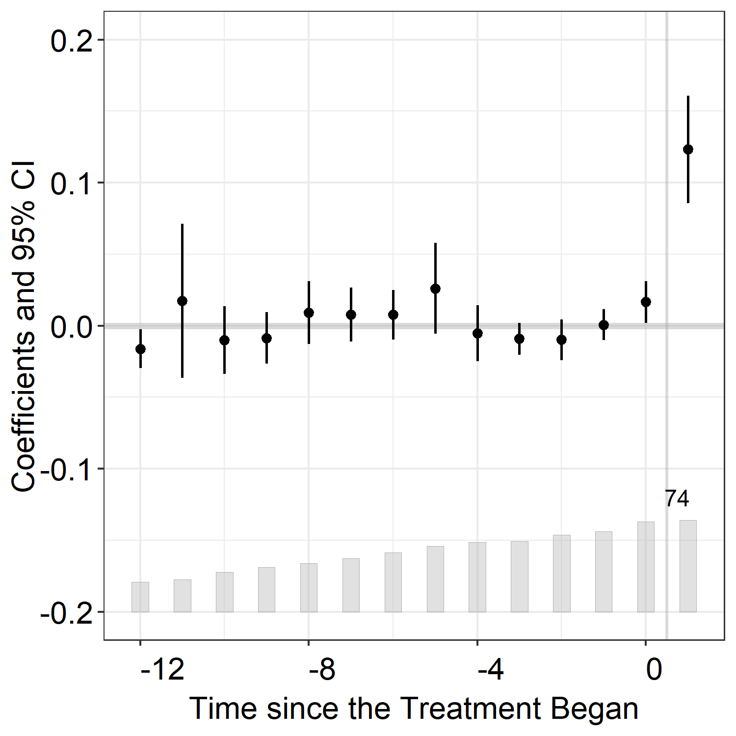
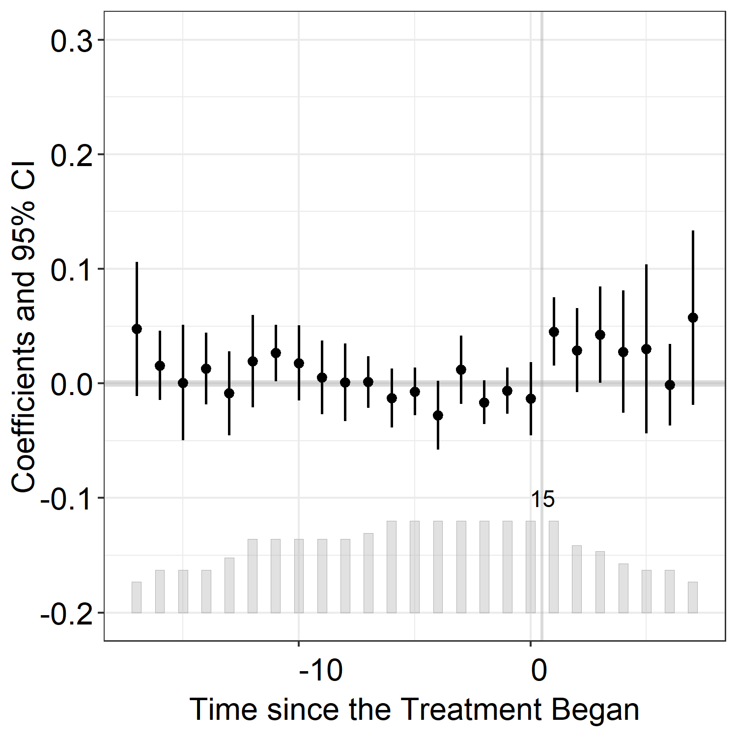
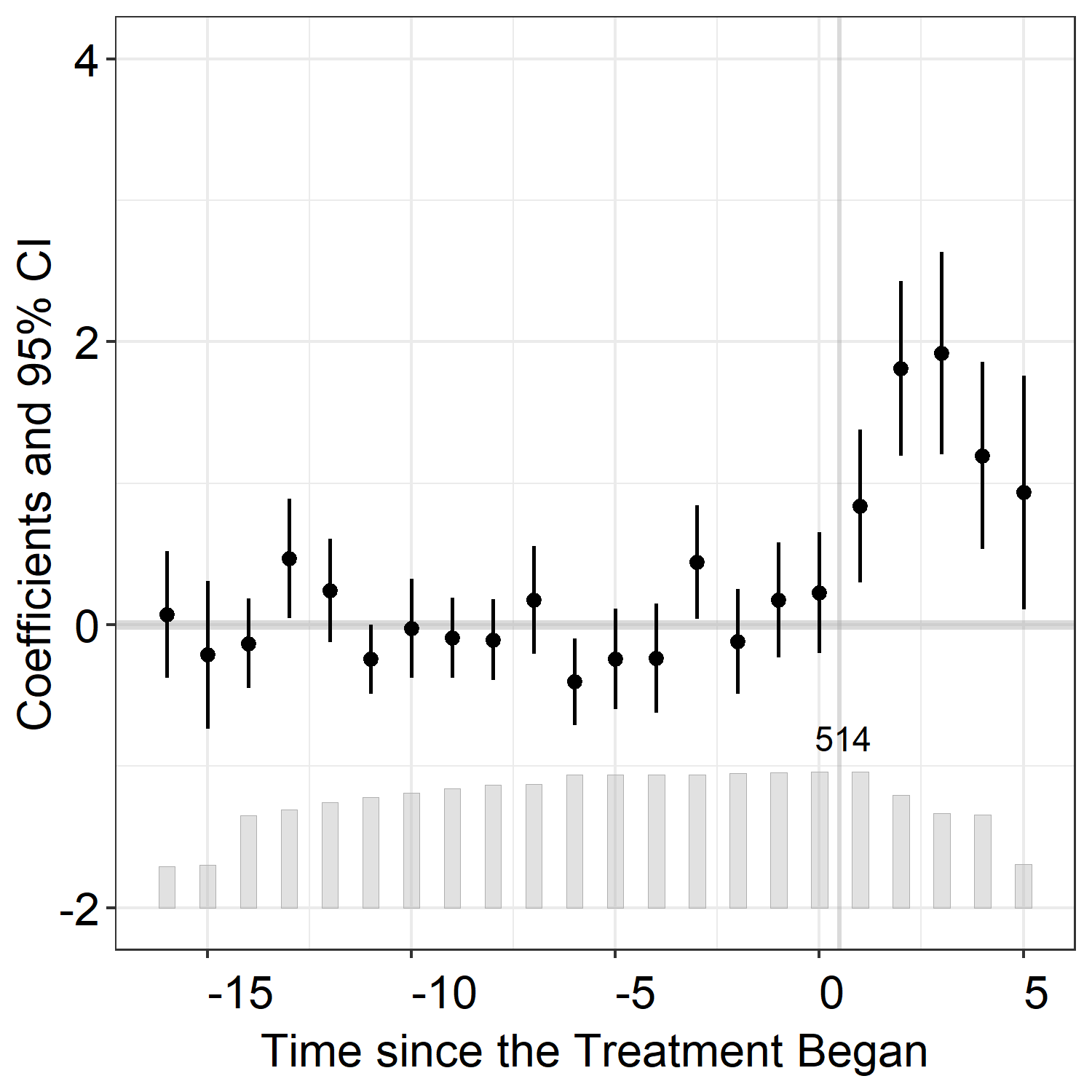
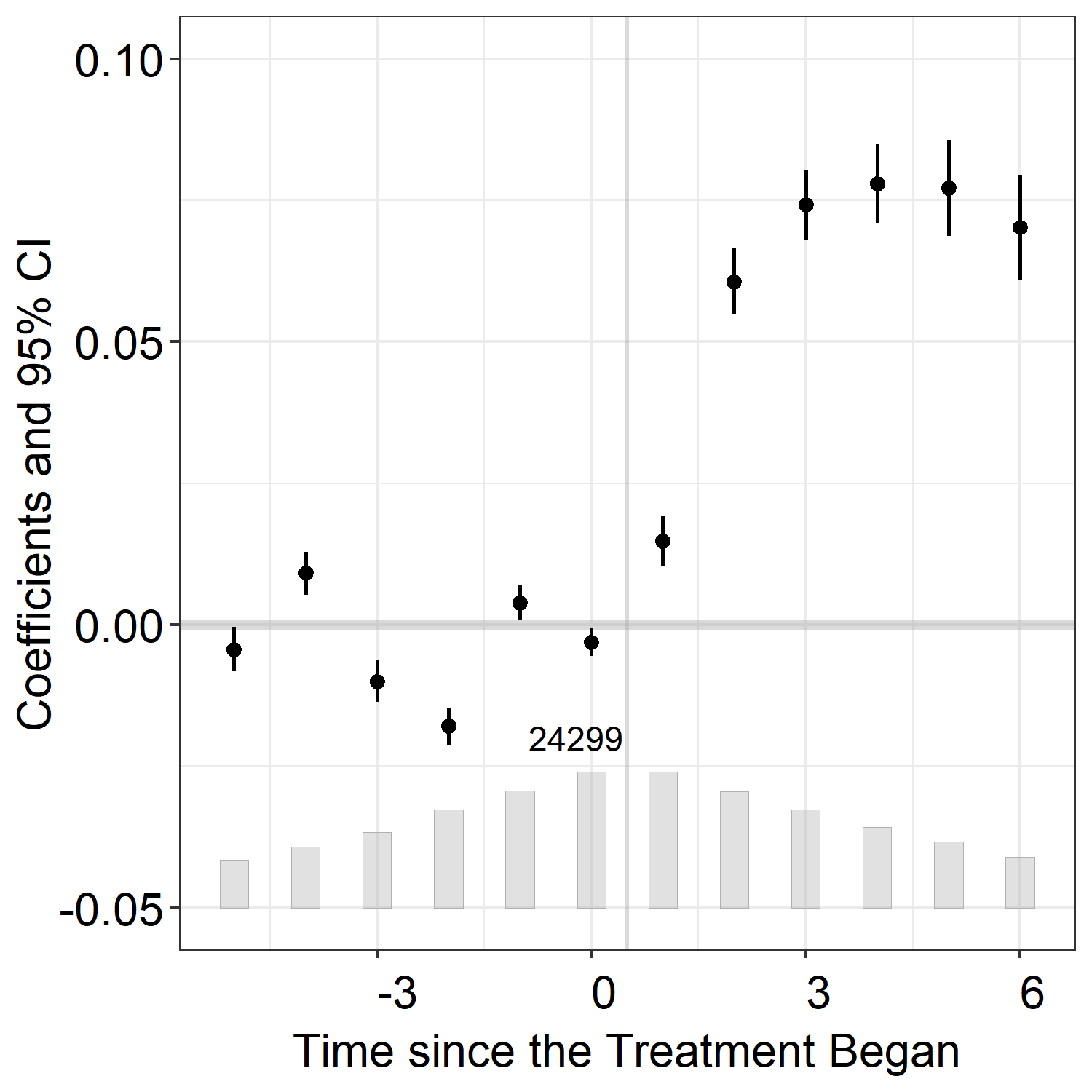
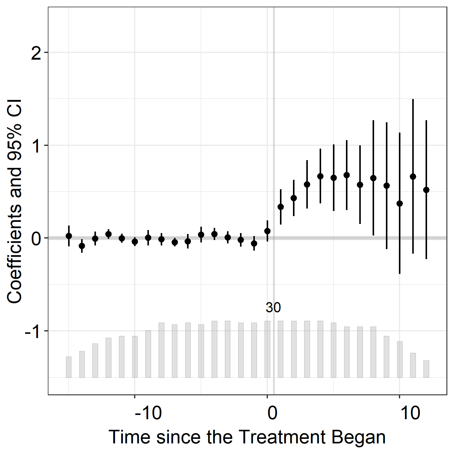
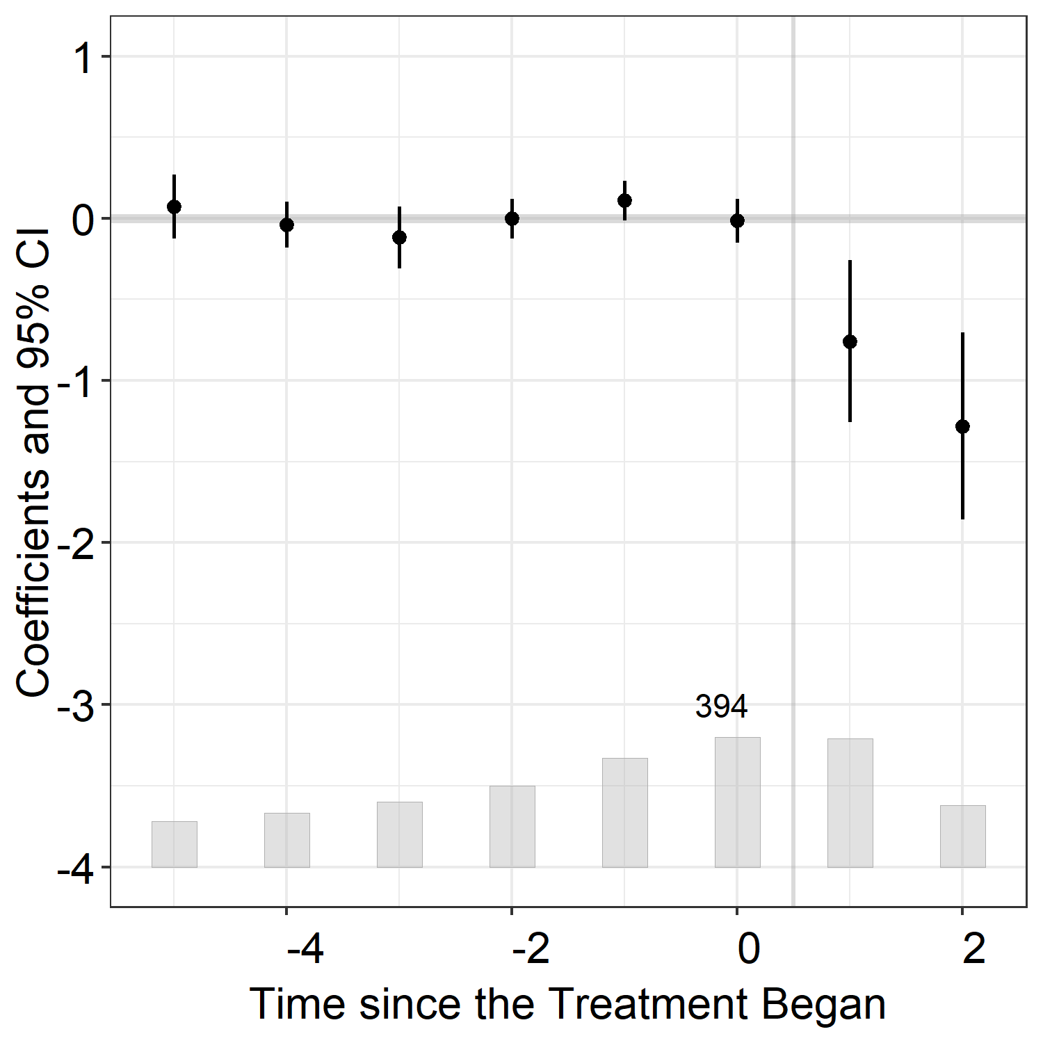
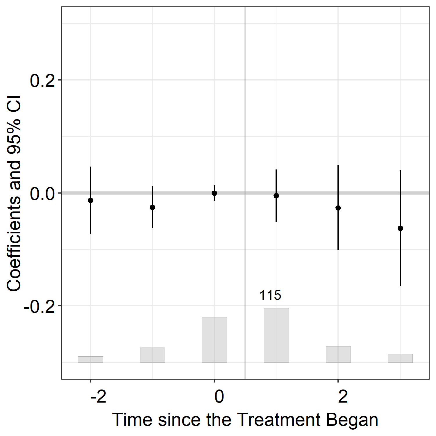
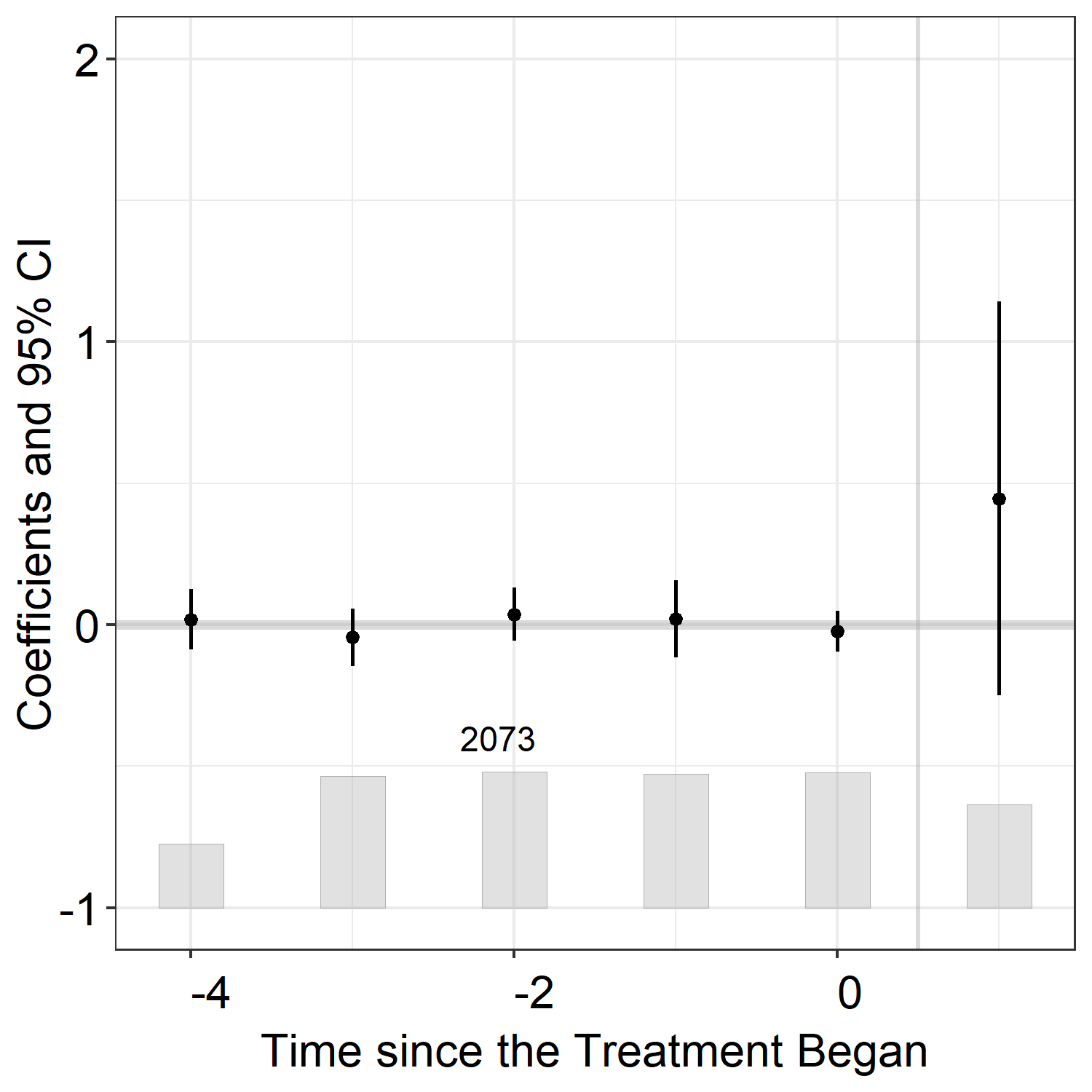
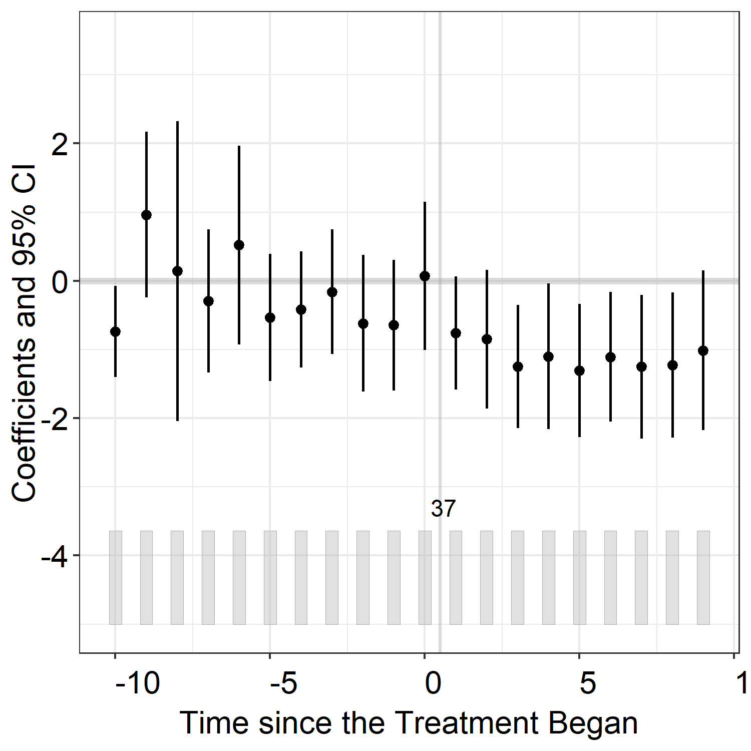
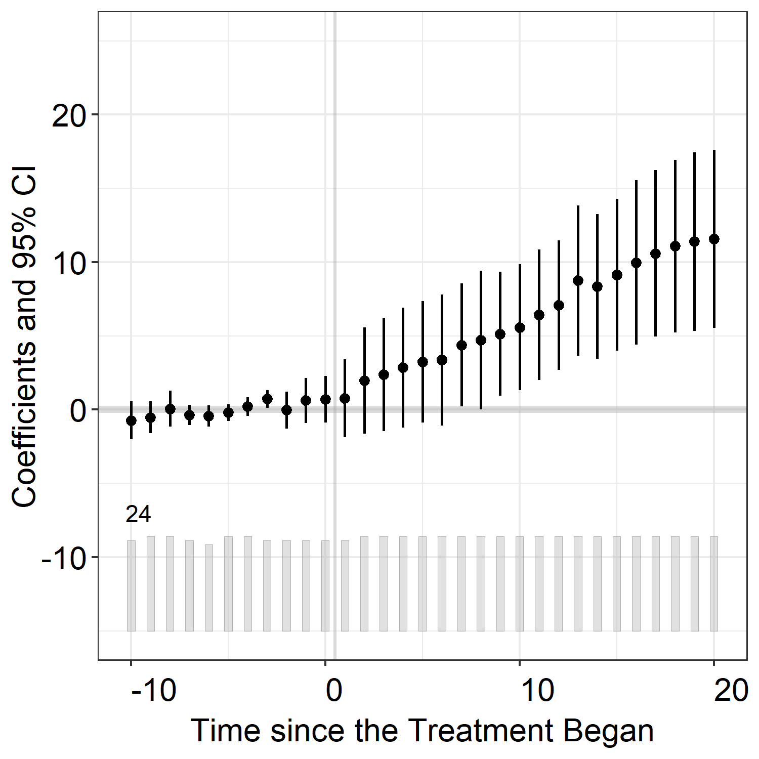
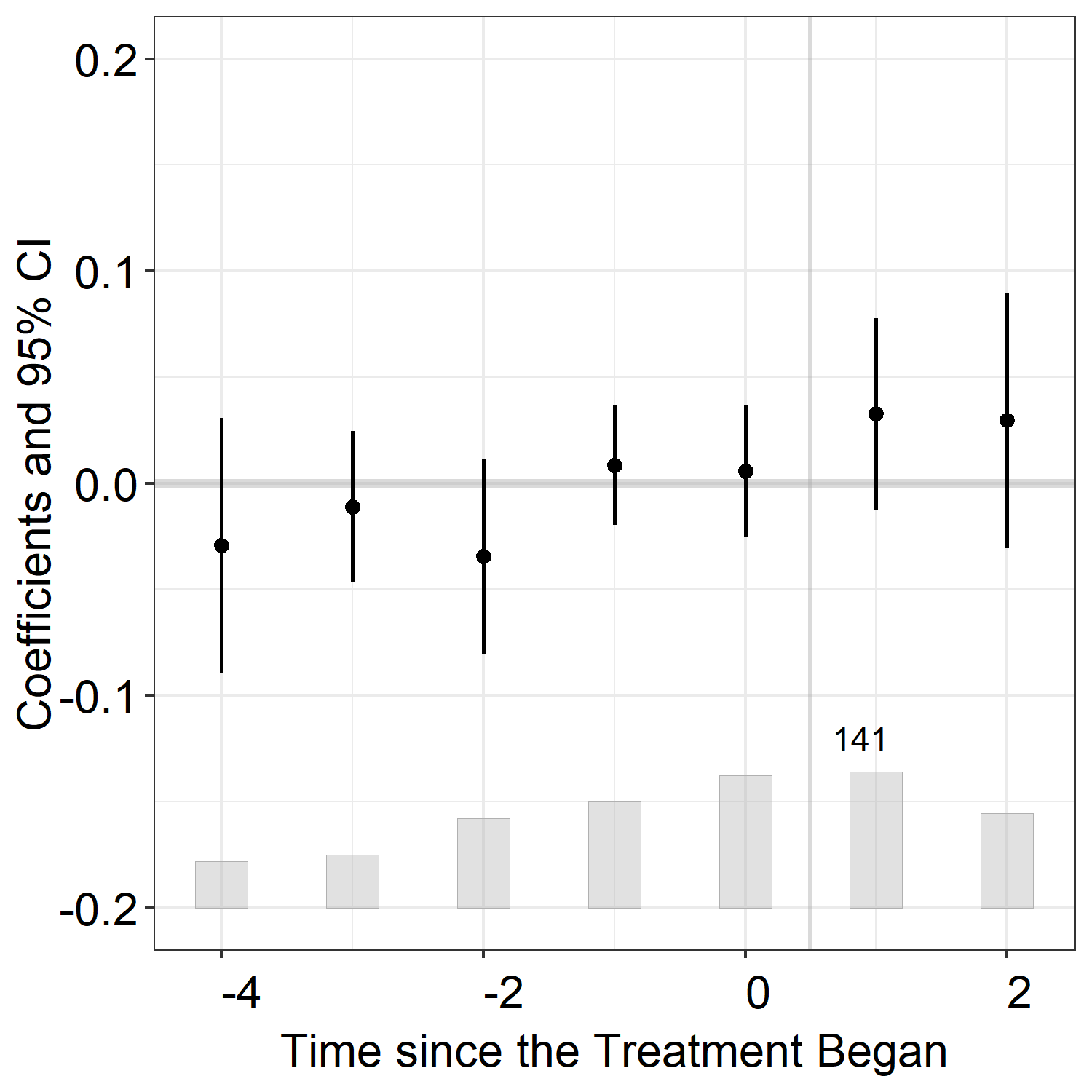
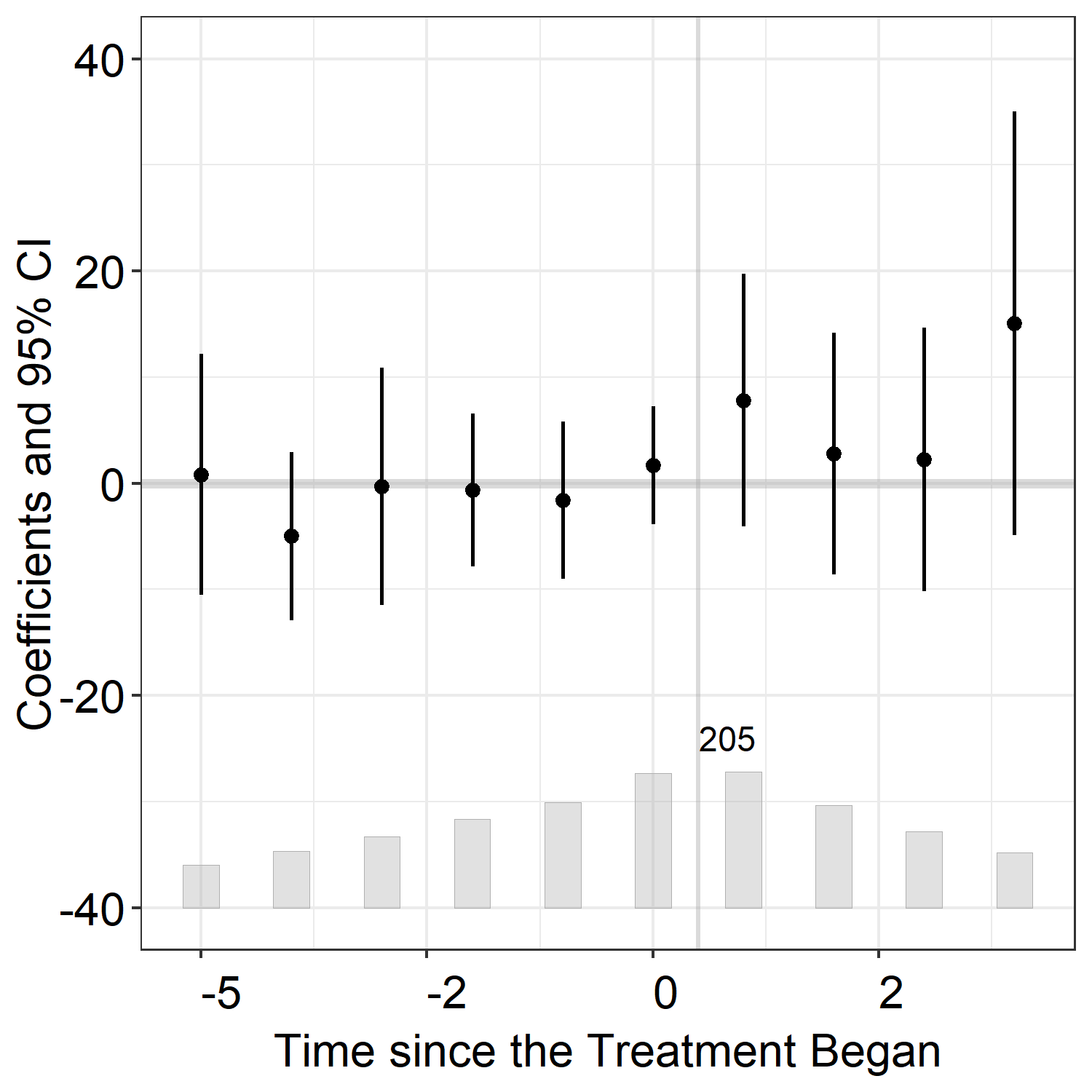
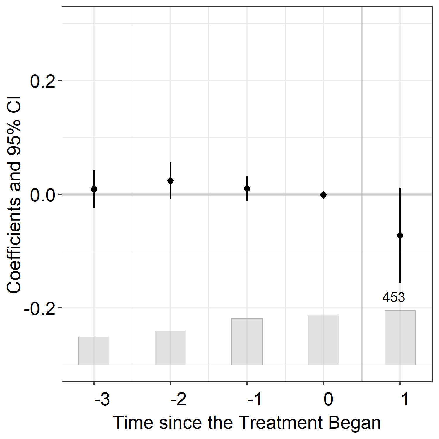
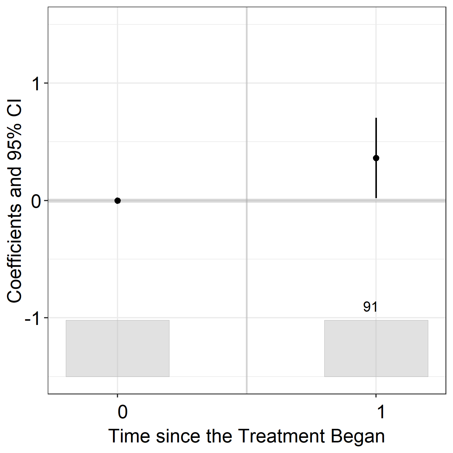
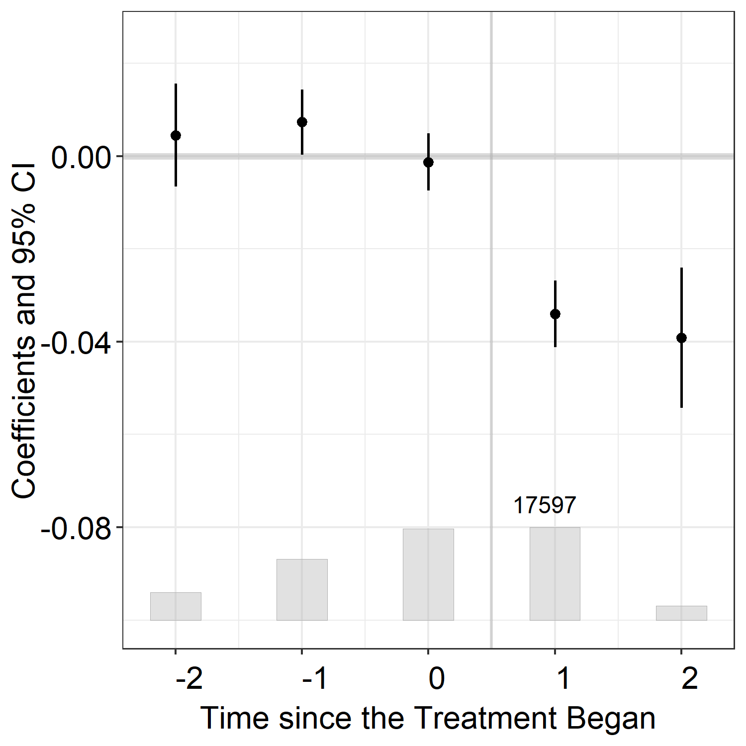
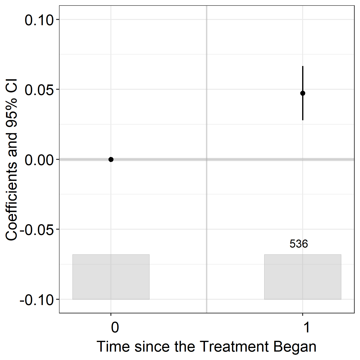
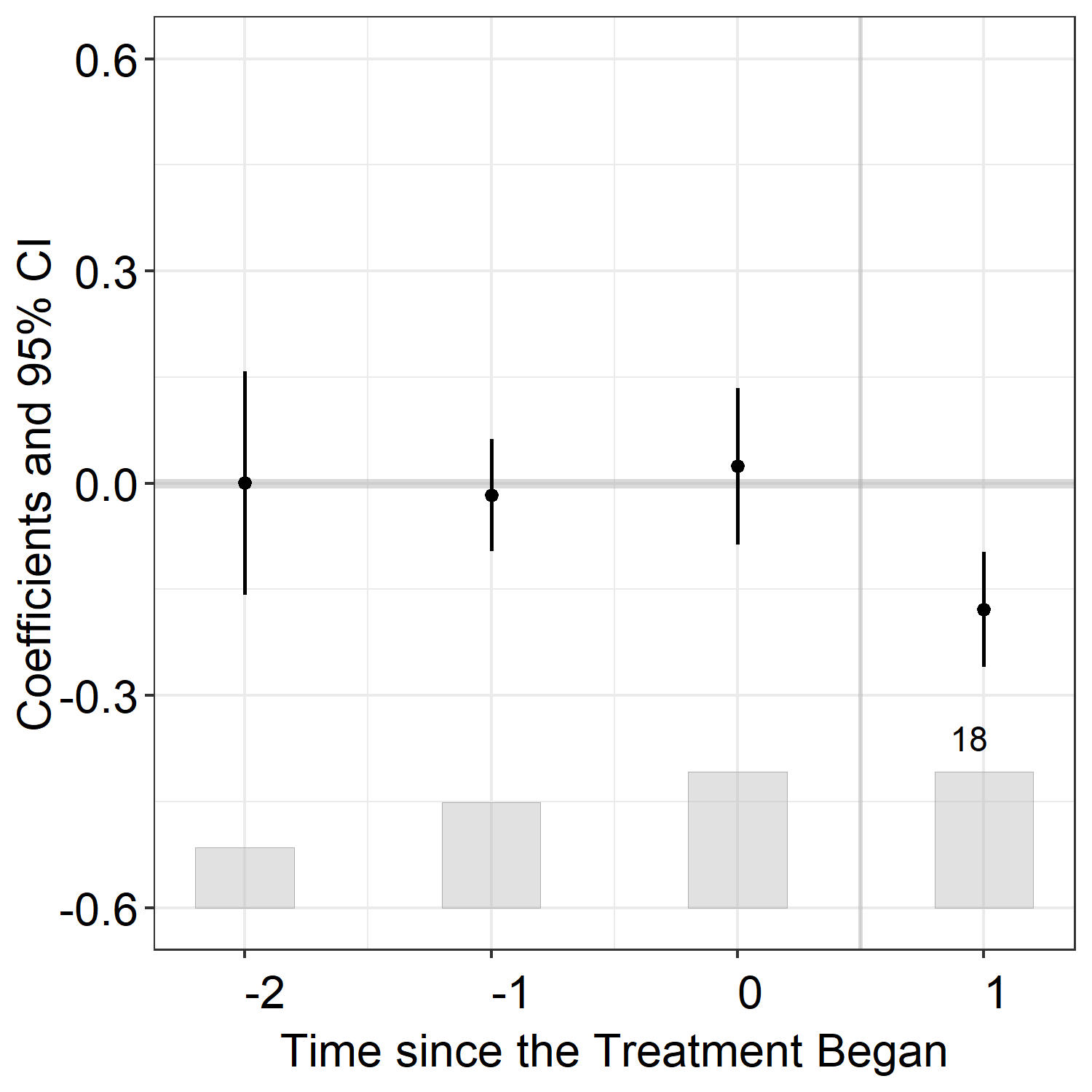
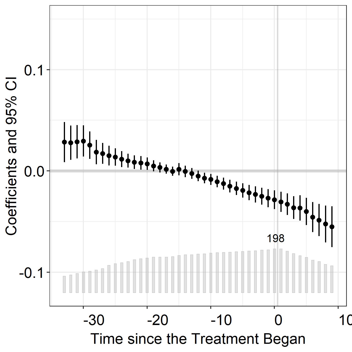
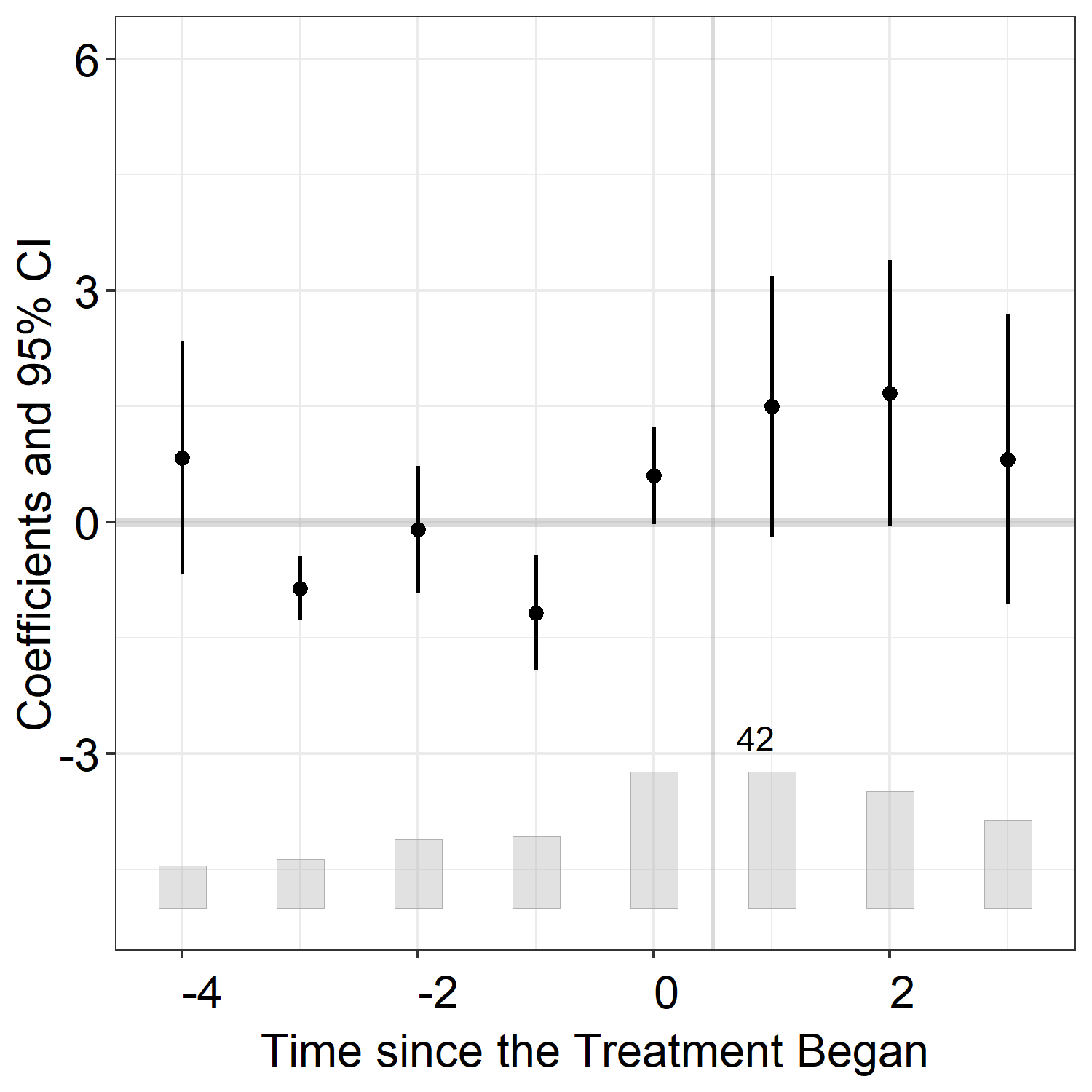
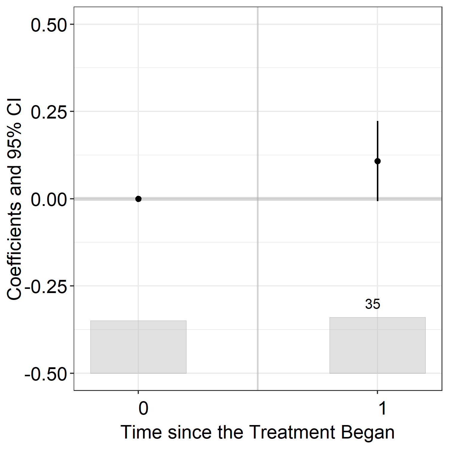
Although the recent methodological literature heavily focuses on the issue of HTE, we report that PTA violations remain a major concern in practice despite having been a well-known pitfall for some time now. Notably, over half of the studies in our sample do not include a DTE/event-study plot of any kind in the main text or SM. In Figure 4, we plot the DTE estimates from FEct. We also report the ATT estimates and their bootstrapped SEs, as well as the $p$-values of the $F$ tests and equivalence tests used to assess the presence of “pretrends.” Due to space limitations, we present the DTE plots from other estimators, as well as results from the placebo tests, in the SM.

Figure 4: Estimated Dynamic Treatment Effects

Beazer and Reuter (2022)
ATT: 24.38 (9.36);
$p$-values: 0.19, 0.71	Bischof and Wagner (2019)
ATT: 0.08 (0.09);
$p$-values: 0.79, 0.49	Bisgaard and Slothuus (2018)
ATT: -0.05 (0.02);
$p$-values: n.a., n.a.	Blair, Christensen and Wirtschafter (2022)
ATT: -0.50 (0.37);
$p$-values: 0.35, 0.49
Bokobza et al. (2022)
ATT: 0.10 (0.03);
$p$-values: 0.04, 0.90	Caughey, Warshaw and Xu (2017)
ATT: 0.01 (0.005);
$p$-values: 0.32, 0.51	Christensen and Garfias (2021)
ATT: 0.04 (0.04);
$p$-values: 0.77, 0.30	Clarke (2020)
ATT: 0.10 (0.02);
$p$-values: 0.29, 0.00
Clayton and Zetterberg (2018)
ATT: 0.19 (0.42);
$p$-values: 0.13, 0.99	Cox and Dincecco (2021)
ATT: 0.44 (0.07);
$p$-values: 0.00, 0.00	Distelhorst and Locke (2018)
ATT: 0.15 (0.05);
$p$-values: 0.29, 0.00	Eckhouse (2022)
ATT: 0.01 (0.01);
$p$-values: 0.21, 0.17
Fouirnaies (2018)
ATT: 0.87 (0.10);
$p$-values: 0.00, 0.00	Fouirnaies and Hall (2018)
ATT: 0.29 (0.02);
$p$-values: 0.15, 0.00	Fouirnaies and Hall (2022)
ATT:-0.26 (0.03);
$p$-values: 0.00, 0.00	Fresh (2018)
ATT: 0.17 (0.07);
$p$-values: 0.86, 0.000
Garfias (2019)
ATT: 0.07 (0.03);
$p$-values: 0.59, 0.42	Grumbach and Sahn (2020)
ATT: 0.14 (0.03);
$p$-values: 0.07, 0.00	Grumbach and Hill (2022)
ATT: 0.033 (0.019);
$p$-values: 0.68, 0.69	Hainmueller and Hangartner (2019)
ATT: 1.51 (0.22);
$p$-values: 0.02, 0.00

Figure 4: Estimated Dynamic Treatment Effects (Cont.)

Hall and Yoder (2022)
ATT: 0.06 (0.003);
$p$-values: 0.00, 0.00	Hirano et al. (2022)
ATT: 0.56 (0.17);
$p$-values: 0.47, 0.00	Jiang (2018)
ATT: -0.87 (0.20);
$p$-values: 0.36, 0.00	Kilborn and Vishwanath (2022)
ATT: 0.05 (0.02);
$p$-values: 0.90, 0.00
Kogan (2021)
ATT: 0.45 (0.43);
$p$-values: 0.86, 0.00	Magaloni, Franco-Vivanco and Melo (2020)
ATT: -2.28 (0.96);
$p$-values: 0.59, 0.65	Paglayan (2022)
ATT: 6.45 (2.01);
$p$-values: 0.67, 0.00	Payson (2020b)
ATT: 0.04 (0.02);
$p$-values: 0.34, 0.35
Payson (2020a)
ATT: 13.04 (7.27);
$p$-values: 0.87, 0.02	Pierskalla and Sacks (2018)
ATT: -0.07 (0.04);
$p$-values: 0.65, 0.00	Ravanilla, Sexton and Haim (2022)
ATT: 0.36 (0.18);
$p$-values: n.a., n.a.	Schafer et al. (2022)
ATT: -0.02 (0.003) ;
$p$-values: 0.07, 0.00
Schubiger (2021)
ATT: 0.05 (0.01);
$p$-values: n.a., n.a.	Schuit and Rogowski (2017)
ATT: -0.16 (0.04) ;
$p$-values: 0.88, 1.00	Trounstine (2020)
ATT: -0.06 (0.01);
$p$-values: 0.00, 0.07	Weschle (2021)
ATT: 1.11 (0.79);
$p$-values: 0.01, 0.58
Zhang et al. (2021)
ATT: 0.11 (0.06);
$p$-values: n.a., n.a.
	Note: We report the estimated ATT and corresponding bootstrap SEs (in parentheses) using FEct. We also provide the $p$-values from the $F$ test and equivalence test. Rejecting the null in the $F$ test indicates potential violations of the PTA while rejecting the null in the equivalence test provides evidence in support of the PTA. These tests are infeasible for four cases with only one pre-treatment period.

The encouraging news is that in over 40% of the studies, we have fairly substantial evidence to attest that the PTA is plausible. In these instances, the DTE estimates in the pre-treatment periods align with zero, and formal statistical tests suggest that the remaining imbalance likely results from randomness in data. Specifically, in these papers the $F$ test does not reject and the equivalence test does reject using the $|\widehat{ATT}|$ as the equivalence threshold, both at the 5% level. In approximately 20% of studies, we find compelling evidence that the PTA is implausible. These are the cases in which we observe a strong pretrend and statistical tests indicate violations of the PTA, i.e. the $F$ test rejects at the 5% level. For the remaining 40% of studies, the results are less clear: We either lack the statistical power or a sufficient number of pretreatment periods to reliably assess the plausibility of the PTA.

HTE-robust estimators do not alter substantive findings but affect power.

To examine the possible impact of the weighting problem caused by HTE, we compared the estimates obtained from the imputation estimator, FEct, to those originally reported. The dissimilarity between the FEct estimates and the original estimates proxies the extent to which the negative weighting problem is consequential in practice.

Figure 5 plots the comparison. The horizontal axis represents the originally reported TWFE estimates, and the vertical axis represents estimates from FEct, both normalized using the originally reported SE. If the point estimates are identical, then the corresponding point should lie exactly on the 45-degree line (dashed). Red solid circles represent studies whose FEct estimates are not significant at the 5% level based on bootstrapped CIs. To assess how the imputation estimator differs from TWFE, we depict the ratio of the FEct estimates to the TWFE estimates, after excluding the always-treated units (ensuring identical sample sets), using solid circles in Figure 6. We also juxtapose the cited TWFE estimates with those omitting the always-treated units, represented by hollow circles. The red circles denote studies where the FEct estimates are not statistically significant at the 5% level.

Figure 5: TWFE vs. Imputation Method

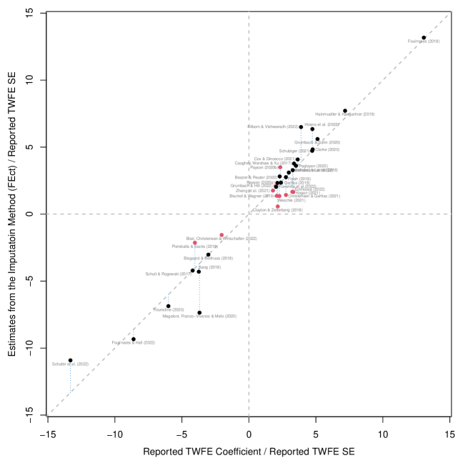
Note: The above figures compare TWFE coefficients and estimates from the imputation method (FEct). Estimates for each application are normalized by the same TWFE SE. The red solid circles represent studies whose ATT estimates from FEct are statistically insignificant at the 5% level based on bootstrapped CIs. Fouirnaies and Hall (2018) and Hall and Yoder (2022) are close to the 45-degree line but not included in the figure as their TWFE $z$-scores are above 15.

We make several observations on Figures 5 and 6. First and foremost, the FEct estimates and the original estimates are highly correlated and always bear the same signs. This suggests that scenarios where accounting for HTE entirely reverses the empirical findings, while theoretically possible, are rare. There are, however, cases where the magnitude of the coefficient changes substantially; the ratios of FEct estimate to TWFE estimate range between 0.25 to 2.081 in our sample. Notably, both the mean and median of these ratios are close to one. This finding suggests that, although there are noticeable differences in individual cases, TWFE does not systematically under- or over-estimates the ATT. Figure 6(a) also shows that the presence of always-treated units is not the primary driver of these differences. When these units are excluded, the TWFE estimates align closely with the reported estimates.

Figure 6: TWFE versus Imputation Method: Estimates and SEs

(a) Changes in Estimates

(b) Changes in SEs

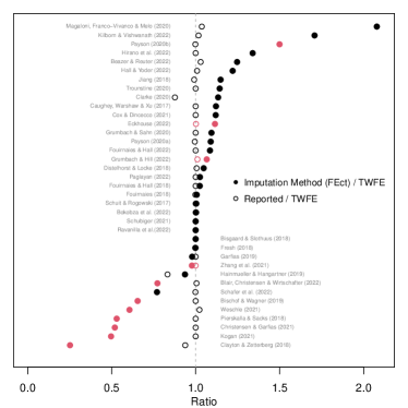
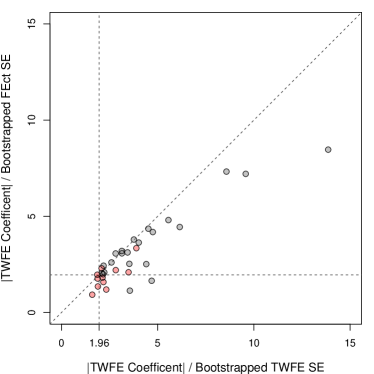
Note: In subfigure (a), solid circles represent the ratios of the estimates from the imputation method (FEct) to TWFE coefficients with always-treated units removed; hollow circles represent the ratios of reported TWFE coefficients to TWFE coefficients with always-treated units removed. Subfigure (b) shows how changes in SEs lead to changes in $z$-scores for the imputation method: the numerators on both axes are the absolute values of the TWFE coefficients (with always-treated observations removed); the denominators are cluster-bootstrapped SEs from TWFE and from FEct, respectively. Statistically insignificant FEct estimates at the 5% level are painted in red in both subfigures.

Alarmingly, when switching from TWFE to FEct, the number of studies that are statistically insignificant at the 5% level rises from one to 11, constituting 28% of all articles. This loss of significance is, at least in part, driven by larger uncertainty estimates. Interestingly, three out of the ten cases that become insignificant have larger FEct estimates compared to their TWFE counterparts. In Figure 6(b), we plot the ratio of the absolute value of the TWFE estimate to the bootstrapped TWFE SEs against the ratio of the absolute value of the TWFE estimate to the bootstrapped FEct SEs. Thus, this visualization exclusively contrasts the SEs derived from each estimator. In the majority of instances, the SEs for FEct are larger than those from TWFE, and the data points for such cases fall below the 45-degree line. While the gap is generally not substantial, at its maximum, the FEct SE can be more than triple the size of the TWFE SEs. In seven cases, when retaining the TWFE point estimate, adopting the SE from FEct would be sufficient to render the result insignificant. It is not surprising that the loss of statistical significance often occurs in studies where the original results have limited power. One takeaway from this finding is that although it is impossible to definitively tell whether the results from any given model are incorrect (especially without knowing the validity of the PTA), the combination of potential biases from HTE and overconfidence of uncertainty estimates may have produced a significant number of false positives, especially when the original estimates carry a high level of uncertainty.

HTE-robust estimators tend to agree with each other.

To compare the behavior of the different HTE-robust estimators, we focus on the seven staggered cases where all estimators are applicable. Figure 7 plots the point estimates obtained from each HTE-robust estimator, in addition to TWFE and stacked DID, all normalized by the reported SE, for these cases. We observe that the estimates from all HTE-robust estimators are qualitatively similar to each other, though there is a noticeable amount of variation. As before, this spread does not change substantive findings for studies with highly substantively significant results, whereas studies whose original $z$ scores are smaller than 3 are much more sensitive to the choice of estimators. Furthermore, though it is difficult to economically present the comparison, our more extensive analyses of each individual paper in the SM show that the DTE estimates from various HTE-robust estimators also generally align with each other and with those from the dynamic specification of the TWFE model.

Figure 7: Comparison of Estimators: Staggered Cases

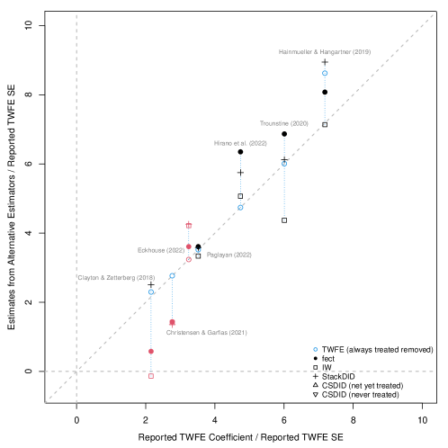
Note: The above figure compares reported coefficients and estimates from various alternative estimators. All seven estimates for each application are normalized by the same reported SE. We multiply the estimates by $Sign(\hat{\delta}^{TWFE}$) for easier visualization; in other words, we flip the signs of all estimates for applications with a negative TWFE estimate.

When it comes to choosing among various HTE-robust estimators, our advice for researchers is to first narrow the selection to those estimators suitable for their specific research context. For instance, if treatment reversal occurs, estimators such as iw and csdid are not applicable. Likewise, if researchers anticipate that long-term effects are more probable than short-term ones, the multiple-DID estimator proposed by de Chaisemartin and D’Haultfœuille (2020) may be less suitable due to their primary focus on short-term effects. Note again that the multiple-DID estimator has a different estimand than the other HTE-robust estimators we discuss: The estimand is partly composed of the (negative of the) effects of exiting treatment, which are ITEs of untreated observations.

We also point out that there is merit to employing multiple HTE-robust estimators. If the estimators are all being used to estimate the same causal estimand, such as the ATT (uniformly weighted over treated observations), they should generally provide qualitatively similar results. This is because, theoretically, they converge to the same target parameter if the identification assumptions hold true. If different results are produced, researchers should be concerned that the PTA is invalid or that the level of precision for which the data allows is insufficient to draw credible conclusions. It may also suggest that there are differential violations of the PTA by different types of units, as these methods vary primarily in how they weight control units.

Other issues.

Our reanalysis highlights several additional issues. First, as we have hinted throughout this section, a large number of studies either lack sufficient statistical power or are on the borderline of being underpowered. According to the authors’ original specifications, one (3%) and 11 (29.7%) studies are not statistically significant at the 5% and 1% levels, respectively. As previously noted, 10 studies lose statistical significance at the 5% level once we apply an HTE-robust estimator. The cause is a combination of a loss of power and, in some cases, smaller point estimates. While only a small fraction of studies in our sample (five articles, 13.5%) employ a bootstrap procedure to estimate SEs or CIs, we observe that the widely practiced cluster-robust SEs typically perform adequately because the numbers of clusters/units are usually fairly large.

Second, the presence of missing values is widespread. Although most methodological work presumes balanced panels without missing data, in reality, many empirical studies encounter varying degrees of data missingness. We plot patterns of treatment status as we do in Figure 2(a) for each study in the SM. Based on these plots, we see that in some studies, the pattern of missingness is either nonrandom or extremely prevalent, which calls into question the reliability and validity of the respective empirical findings.

Third, we perform carryover effect tests for all studies that feature treatment reversals. If this test fails, it suggests that the treatment effects persist beyond the treatment periods. Among 22 articles, five reject the null hypothesis of no carryover effects at 5%. LWX (2022) note that the presence of carryover effects for a limited number of periods is less concerning, as researchers can recode treatment to persist for some time after a unit transitions out of treatment. By adopting this guideline, we observe that carryover effects do not substantially alter the findings in most studies. Specifically, estimates are similar in magnitude, and results initially deemed statistically significant continue to hold their statistical significance (Figure A7 in the SM). Nevertheless, we recommend that researchers make it a practice to check for potential carryover effects, considering the low cost of conducting such tests and adjustments.

Many studies also exhibit sensitivity to model specifications. When we incorporate an LDV or ULT into the authors’ original specifications, a large number of studies lose their statistical significance (29% and 41% respectively). While it is true that such models may be vulnerable to additional biases, such as the Nickell bias in short dynamic panels, and the additional parameters reduce efficiency, these results underscore that a significant number of empirical findings in the literature rely heavily on the modeling assumptions. Hence, we recommend researchers carefully assess the robustness of their findings using different model specifications, possibly in combination with HTE-robust estimators. We reserve a more careful and rigorous analysis of this issue for future studies.

Relatedly, some studies that we exclude from our sample employ one-way FE or FE at a level different from that at which treatment is assigned. Many of these findings do not hold when we reanalyze them using a TWFE model. We should clarify that this does not imply that the original results are not credible; rather, it underlines the fact that these models operate under distinct identification assumptions, and there is substantial variation in how much consideration authors give to this point. We notice that some studies do not provide a rationale for their choice to use one-way fixed effects, while others explicitly outline the type of unobserved confounders they intend to control for. In one instance, the authors inaccurately label their specification as a DID design. We emphasize that TWFE and DID are generally not equivalent. This difference becomes even more pronounced when the fixed effects are not assigned at the level of treatment.

Summary.

In Table 4 below, we summarize the main findings of our reanalysis. The first three columns indicate the proportion of studies in each journal, and across all journals, that have potential PTA violations. The numbers represent the proportion of studies where the null hypothesis is rejected at the 5% significance level for the $F$ test and the placebo test and not rejected for the equivalence test. Across all journals, around a quarter of studies reject the null hypothesis using the $F$ test, with slightly fewer rejecting when using the placebo test, indicating potential PTA violations. Note, though, that failure to reject to reject may result from insufficient power. In 47% of the cases, the equivalence test fails to reject the null hypothesis using $|\widehat{ATT}|$ as the threshold, implying that for these studies we cannot confidently state that the pre-treatment residual averages lie within a narrow range defined by the estimated ATT.

Table 4: Summary of Findings

	Potential PTA violations			Consequence of HTE		Insufficient power
	(1)	(2)	(3)	(4)	(5)	(6)	(7)
	$F$ test	Placebo test	Equiv. test	FEct-TWFE	FEct-TWFE	TWFE not	FEct not
Journal	reject null	reject null	not reject null	Ratio $<0.8$	Ratio $<0.5$	reject null	reject null
APSR (6)	0.33	0.33	0.50	0.00	0.00	0.00	0.17
AJPS (12)	0.25	0.17	0.42	0.15	0.00	0.00	0.15
JOP (19)	0.19	0.12	0.50	0.32	0.11	0.05	0.42
All (37)	0.24	0.17	0.47	0.21	0.05	0.03	0.29
Note: A null is deemed being rejected if $p<0.05$. “Ratio” refers to the ratio of the FEct estimate to TWFE estimate for the average effect. Four studies with only a single pre-treatment period are not included in the summary statistics in columns (1)–(3).

Columns (4) and (5) show the ratio of the FEct estimator to the TWFE estimator, which proxies the consequences of HTE. Across all journals, in 21% of studies, this ratio is less than 0.8, and in 5% of studies, the ratio is less than 0.5, indicating that while HTE might be a significant concern theoretically, its practical influence on yielding qualitatively different findings may not be as substantial as the existing literature might suggest. Lastly, columns (6) and (7) show the proportion of studies in which the null hypothesis of no effect is not rejected by TWFE and FEct respectively. When employing the TWFE method, this happens in 3% of the studies across all journals; however, when the FEct estimator is utilized, this number increases to 29%, suggesting many studies in our sample are potentially underpowered.

When we synthesize these multiple lines of evidence, we find that 12 studies (or 32% of our sample) provide strong evidence supporting the plausibility of the PTA—reflected by the rejection of the equivalence test—and distinguish the ATT from zero with sufficient statistical power. If we instead consider studies where the $F$ test has a $p$-value greater than 0.05 (acknowledging that the $F$ test is often underpowered), this number increases to 16 studies (42%).

We emphasize that our goal is not to pass judgment on each individual paper, but rather to understand the state of the literature at large. We thus do not attempt to label ambiguous cases that neither suffer from clear PTA violations and weighting problems nor provide strong evidence to the contrary. Similarly, we do not tabulate subjective calls on whether pretrends look “good” or “bad,” despite our advice for researchers to do so themselves. In practice, when readers are attempting to evaluate the strength of evidence for a specific study, we remind readers that credibility is not binary and urge readers to take a holistic view of the evidence.

6.  What To Do and (Not) To Do with Causal Panel Analysis

We conclude by sharing practical advice based on both our findings and our experiences conducting a vast number of replications and reanalyses using observational panel data. Table 5 summarizes these lessons. The first consideration is the research design. Our results echo the advice from Rubin (2008): “Design trumps analysis,” and it is imperative to understand the underlying assignment mechanism. While fixed effects allow us to control for certain unobserved confounders, this comes at the cost of strong assumptions about functional form as well as the dynamics between the treatment and outcome, such as the absence of anticipation, feedback, and time-varying confounders. If a glaring violation is already known to exist at this stage, a new identification strategy is needed.

If confounding at the unit level is a major concern and the PTA or strict exogeneity is plausible, we encourage researchers to plot the data at hand in order to understand the patterns in treatment assignment and missing data. Ideally, treatment assignments will vary both by unit and time. If the majority of variation occurs over time (unit) with little or no variation between units at any given time period (or across time within a given unit), the TWFE estimand will be dominated by impermissible comparisons and thus potentially highly biased. Furthermore, HTE-robust estimators will estimate the treatment effect using very little data and thus be underpowered. Equally important is the need for researchers to understand the degree and possible origins of data missingness prior to initiating statistical analysis. If missingness does not seem to be random, or if it is too prevalent, leaving insufficient meaningful variation in the data, researchers should consider halting the analysis at this stage. Indeed, proceeding under these circumstances can lead to biased estimates and unreliable conclusions. Just as in the cross-sectional case, plotting the raw data can also help researchers to spot outliers and highly skewed distributions. The time dimension of panel data creates unique concerns about the distribution of the data: If the outcome variable is highly serially correlated, further transformation such as first-difference or adding LDVs may be needed (Beck and Katz, 2011), as our analysis has shown many models are sensitive to such modeling choices.

Table 5: Do’s and Don’ts with Causal Panel Analysis

	Do’s	Don’ts
Design trumps analysis	Start empirical analysis with a research design; stop if “feedback” from past outcomes to treatment assignment is a major concern	Start empirical analysis by blindly running regressions
Discussion of designs	Clearly specify designs and their corresponding identification assumptions	Equate designs with outcome models
Plot raw data	Plot raw data to better understand the research setting, missingness, sources of variations in the treatment and outcome variables, and whether some variables need to be transformed first because of nonstationarity, outliers, or highly skewed distributions	Run regressions without inspecting and visualizing the data
Estimation	Choose HTE-robust estimators and always plot the estimated DTE	Choose models solely based on your beliefs; report regression coefficients only; no results visualization or diagnostics
Diagnostics	Conduct both visual and statistical tests to gauge whether the PTA and the no-carryover-effect assumption are plausible
Quantify uncertainties	Cluster SEs at the level of unit or treatment assignment, whichever is high; use cluster-bootstrap procedures when the number of clusters is small (e.g., $<50$)	Use unclustered SEs or use clustered SEs when the number of clusters is small
Explore HTE	Explore HTE along time, unit (cohort), and theoretically important pretreatment covariates with flexible estimation strategies; visualize your findings	Do not explore HTE or do so through rigid parametric models

At the stage of estimation, we recommend choosing an estimator that is robust to HTE. Although our study reveals that most results are not sensitive to choice of estimators, this is an empirical observation and not a theoretical guarantee. A non-negligible minority of HTE-robust estimates in our sample are substantively different from the TWFE, and it is not sufficient to simply hope that one’s own study does not fall within this group. There is a loss of efficiency, but we argue this is an acceptable price. Moreover, it is always possible to include a potentially more precise TWFE estimate in addition to the main, HTE-robust estimate when power is a concern and effects are close to homogeneous (or, if effects are heterogeneous, weighting does not seem to be an issue).

We recommend using the chosen estimator to estimate and plot DTE, then conducting both statistical tests and a visual inspection to assess the validity of strict exogeneity or the PTA. While we focus on statistical tests and hesitate to publish ‘results’ of visual inspections in our systematic analysis, our omission of the latter is due solely to its subjective nature and does not imply its irrelevance. While statistical tests are useful, they are not sufficient to replace visual inspections for two main reasons. First, all statistical tests risk making errors. Second, visual inspections can reveal a lot about the nature and severity of a pretrend that is masked by a simple $p$-value; the $F$ test for a study with a clear, monotonic pretrend but a small sample size may return a much larger $p$-value than the one for a very-large-$N$ study with a similar or more mild pretrend. The existence of a pretrend may reflect a fundamental flaw in the study design. Researchers may attempt to resolve the issue in several ways—for example, by conditioning on additional (pre-treatment) covariates, or by using a more flexible estimator. It may also involve small alterations to the research design, such as a more careful selection of the “control” group. This strategy is also related to the choice of estimator, which differs in their choices of comparison groups. We urge practitioners to be transparent about the results of these tests and the DTE (event study) plots, as well as any measures taken as a result of seeing them. The reader can then determine for themselves if and how the estimates should update their beliefs about the answers to the research question being investigated. We also recommend checking for carryover effects, whose existence may be addressed by recoding the treatment so that it persists for some time after a unit switches out of treatment.

For statistical inference, researchers should employ cluster-robust SEs when the number of clusters is large (e.g., exceeds $50$) or a cluster-bootstrap procedure when the number of clusters is relatively small. The selection of the level on which to cluster should be based on the level of time-series units or the level of treatment assignment, opting for the higher of the two. Recent research indicates that clustering at the level of treatment assignment can be considered a conservative approach if potential outcome variations are primarily driven by idiosyncratic errors (Abadie et al., 2023); however, we believe this strategy is a safer route for conducting inference, as it can help minimize the occurrence of false positives because it is usually difficult for researchers to perfectly determine the primary sources of these variations.

Panel data provides unique opportunities that can assist social scientists in answering difficult causal questions. Such data, particularly when operating under the PTA, also presents its own set of challenges. Our findings and recommendations should not dissuade researchers from employing panel data for causal analysis. Rather, we hope they guide researchers in carrying out this task in a more transparent and credible manner. To facilitate this process, we develop an open-source package, paneltools, in R, along with a detailed tutorial (https://yiqingxu.org/tutorials/panel.html), for researchers to implement all the procedures used in this paper.

References

- (1)
- Abadie et al. (2023) Abadie, Alberto, Susan Athey, Guido W Imbens and Jeffrey M Wooldridge. 2023. “When should you adjust standard errors for clustering?” Quarterly Journal of Economics 138(1):1–35.
- Arkhangelsky and Imbens (2022) Arkhangelsky, Dmitry and Guido W Imbens. 2022. “Doubly robust identification for causal panel data models.” The Econometrics Journal 25(3):649–674.
- Arkhangelsky et al. (2021) Arkhangelsky, Dmitry, Guido W Imbens, Lihua Lei and Xiaoman Luo. 2021. “Double-Robust Two-Way-Fixed-Effects Regression For Panel Data.”.
- Aronow, Samii and Wang (2020) Aronow, Peter M, Cyrus Samii and Ye Wang. 2020. “Design-Based Inference for Spatial Experiments with Interference.”.
- Athey and Imbens (2022) Athey, Susan and Guido W Imbens. 2022. “Design-based analysis in difference-in-differences settings with staggered adoption.” Journal of Econometrics 226(1):62–79.
- Bai and Ng (2021) Bai, Jushan and Serena Ng. 2021. “Matrix completion, counterfactuals, and factor analysis of missing data.” Journal of the American Statistical Association 116(536):1746–1763.
- Baker, Larcker and Wang (2022) Baker, Andrew C, David F Larcker and Charles CY Wang. 2022. “How much should we trust staggered difference-in-differences estimates?” Journal of Financial Economics 144(2):370–395.
- Beazer and Reuter (2022) Beazer, Quintin H. and Ora John Reuter. 2022. “Do Authoritarian Elections Help the Poor? Evidence from Russian Cities.” Journal of Politics 84:437–454.
- Beck and Katz (1995) Beck, Nathaniel and Jonathan N Katz. 1995. “What to Do (and Not to Do) with Time-Series Cross-Section Data.” American Political Science Review 89(3):634–647.
- Beck and Katz (2001) Beck, Nathaniel and Jonathan N Katz. 2001. “Throwing Out the Baby with the Bath Water: A Comment on Green, Kim, and Yoon.” International Organization 55(2):487–495.
- Beck and Katz (2011) Beck, Nathaniel and Jonathan N Katz. 2011. “Modeling Dynamics in Time-Series–Cross-Section Political Economy Data.” Annual Review of Political Science 14(1):331–352.
- Bertrand, Duflo and Mullainathan (2004) Bertrand, Marianne, Esther Duflo and Sendhil Mullainathan. 2004. “How Much Should We Trust Differences-in-Differences Estimates?” Quarterly Journal of Economics 119(1):249–275.
- Bischof and Wagner (2019) Bischof, Daniel and Markus Wagner. 2019. “Do Voters Polarize When Radical Parties Enter Parliament?” American Journal of Political Science 63(4):888–904.
- Bisgaard and Slothuus (2018) Bisgaard, Martin and Rune Slothuus. 2018. “Partisan Elites as Culprits? How Party Cues Shape Partisan Perceptual Gaps.” American Journal of Political Science 62(2):456–469.
- Blackwell and Glynn (2018) Blackwell, Matthew and Adam Glynn. 2018. “How to Make Causal Inferences with Time-Series Cross-Sectional Data Under Selection on Observables.” American Political Science Review 112(2):1067–1082.
- Blair, Christensen and Wirtschafter (2022) Blair, Graeme, Darin Christensen and Valerie Wirtschafter. 2022. “How Does Armed Conflict Shape Investment? Evidence from the Mining Sector.” Journal of Politics 84:116–133.
- Bokobza et al. (2022) Bokobza, Laure, Suthan Krishnarajan, Jacob Nyrup, Casper Sakstrup and Lasse Aaskoven. 2022. “The Morning After: Cabinet Instability and the Purging of Ministers after Failed Coup Attempts in Autocracies.” Journal of Politics 84:1437–1452.
- Borusyak, Jaravel and Spiess (2023) Borusyak, Kirill, Xavier Jaravel and Jann Spiess. 2023. “Revisiting Event Study Designs: Robust and Efficient Estimation.” Review of Economic Studies (forthcoming) .
- Callaway and Sant’Anna (2021) Callaway, Brantly and Pedro HC Sant’Anna. 2021. “Difference-in-differences with multiple time periods.” Journal of Econometrics 225(2):200–230.
- Callaway and Karami (2023) Callaway, Brantly and Sonia Karami. 2023. “Treatment effects in interactive fixed effects models with a small number of time periods.” Journal of Econometrics 233(1):184–208.
- Cameron, Gelbach and Miller (2008) Cameron, A Colin, Jonah B Gelbach and Douglas L Miller. 2008. “Bootstrap-based Improvements for Inference with Clustered Errors.” Review of Economics and Statistics 90(3):414–427.
- Caughey, Warshaw and Xu (2017) Caughey, Devin, Christopher Warshaw and Yiqing Xu. 2017. “Incremental democracy: The policy effects of partisan control of state government.” Journal of Politics 79(4):1342–1358.
- Christensen and Garfias (2021) Christensen, Darin and Francisco Garfias. 2021. “The politics of property taxation: Fiscal infrastructure and electoral incentives in Brazil.” Journal of Politics 83(4):1399–1416.
- Clarke (2020) Clarke, Andrew J. 2020. “Party Sub-Brands and American Party Factions.” American Journal of Political Science 64(3):452–470.
- Clayton and Zetterberg (2018) Clayton, Amanda and Pär Zetterberg. 2018. “Quota shocks: Electoral gender quotas and government spending priorities worldwide.” Journal of Politics 80(3):916–932.
- Cox and Dincecco (2021) Cox, Gary W and Mark Dincecco. 2021. “The budgetary origins of fiscal-military prowess.” Journal of Politics 83(3):851–866.
- de Chaisemartin and D’Haultfœuille (2017) de Chaisemartin, Clément and Xavier D’Haultfœuille. 2017. “Fuzzy Differences-in-Differences.” Review of Economic Studies 85(2):999–1028.
- de Chaisemartin and D’Haultfœuille (2020) de Chaisemartin, Clément and Xavier D’Haultfœuille. 2020. “Two-way Fixed Effects Estimators with Heterogeneous Treatment Effects.” American Economic Review 110(9):2964–2996.
- Distelhorst and Locke (2018) Distelhorst, Greg and Richard M. Locke. 2018. “Does Compliance Pay? Social Standards and Firm-Level Trade.” American Journal of Political Science 62(3):695–711.
- Eckhouse (2022) Eckhouse, Laurel. 2022. “Metrics Management and Bureaucratic Accountability: Evidence from Policing.” American Journal of Political Science 66(2):385–401.
- Eggers et al. (2015) Eggers, Andrew C, Anthony Fowler, Jens Hainmueller, Andrew B Hall and James M Snyder Jr. 2015. “On the validity of the regression discontinuity design for estimating electoral effects: New evidence from over 40,000 close races.” American Journal of Political Science 59(1):259–274.
- Fouirnaies (2018) Fouirnaies, Alexander. 2018. “When Are Agenda Setters Valuable?” American Journal of Political Science 62(1):176–191.
- Fouirnaies and Hall (2018) Fouirnaies, Alexander and Andrew B. Hall. 2018. “How Do Interest Groups Seek Access to Committees?” American Journal of Political Science 62(1):132–147.
- Fouirnaies and Hall (2022) Fouirnaies, Alexander and Andrew B. Hall. 2022. “How Do Electoral Incentives Affect Legislator Behavior? Evidence from U.S. State Legislatures.” American Political Science Review 116:662–676.
- Fresh (2018) Fresh, Adriane. 2018. “The Effect of the Voting Rights Act on Enfranchisement: Evidence from North Carolina.” Journal of Politics 80(2):713–718.
- Garfias (2019) Garfias, Francisco. 2019. “Elite coalitions, limited government, and fiscal capacity development: Evidence from bourbon Mexico.” Journal of Politics 81(1):95–111.
- Goodman-Bacon (2021) Goodman-Bacon, Andrew. 2021. “Difference-in-differences with variation in treatment timing.” Journal of Econometrics 225(2):254–277.
- Green, Kim and Yoon (2001) Green, Donald P, Soo Yeon Kim and David H Yoon. 2001. “Dirty Pool.” International Organization 55(2):441–468.
- Grumbach and Sahn (2020) Grumbach, Jacob M. and Alexander Sahn. 2020. “Race and Representation in Campaign Finance.” American Political Science Review 114(1):206–221.
- Grumbach and Hill (2022) Grumbach, Jacob M. and Charlotte Hill. 2022. “Rock the Registration: Same Day Registration Increases Turnout of Young Voters.” Journal of Politics 84:405–417.
- Hainmueller and Hangartner (2019) Hainmueller, Jens and Dominik Hangartner. 2019. “Does direct democracy hurt immigrant minorities? Evidence from naturalization decisions in Switzerland.” American Journal of Political Science 63(3):530–547.
- Hainmueller, Mummolo and Xu (2019) Hainmueller, Jens, Jonathan Mummolo and Yiqing Xu. 2019. “How much should we trust estimates from multiplicative interaction models? Simple tools to improve empirical practice.” Political Analysis 27(2):163–192.
- Hall and Yoder (2022) Hall, Andrew B. and Jesse Yoder. 2022. “Does Homeownership Influence Political Behavior? Evidence from Administrative Data.” Journal of Politics 84:351–366.
- Hirano et al. (2022) Hirano, Shigeo, Jaclyn Kaslovsky, Michael P. Olson and James M. Snyder. 2022. “The Growth of Campaign Advertising in the United States, 1880–1930.” Journal of Politics 84:1482–1496.
- Imai and Kim (2019) Imai, Kosuke and In Song Kim. 2019. “When Should We Use Unit Fixed Effects Regression Models for Causal Inference with Longitudinal Data?” American Journal of Political Science 63(2):467–490.
- Imai, Kim and Wang (2023) Imai, Kosuke, In Song Kim and Erik H Wang. 2023. “Matching methods for causal inference with time-series cross-sectional data.” American Journal of Political Science 67(3):587–605.
- Jiang (2018) Jiang, Junyan. 2018. “Making Bureaucracy Work: Patronage Networks, Performance Incentives, and Economic Development in China.” American Journal of Political Science 62(4):982–999.
- Kilborn and Vishwanath (2022) Kilborn, Mitchell and Arjun Vishwanath. 2022. “Public money talks too: How public campaign financing degrades representation.” American Journal of Political Science 66(3):730–744.
- King (2001) King, Gary. 2001. “Proper Nouns and Methodological Propriety: Pooling Dyads in International Relations Data.” International Organization 55(2):497–507.
- Kogan (2021) Kogan, Vladimir. 2021. “Do welfare benefits pay electoral dividends? Evidence from the national food stamp program rollout.” Journal of Politics 83(1):20–70.
- Lal et al. (2023) Lal, Apoorva, Mac Lockhart, Yiqing Xu and Ziwen Zu. 2023. “How much should we trust instrumental variable estimates in political science? Practical advice based on over 60 replicated studies.” arXiv preprint arXiv:2303.11399 .
- Lall (2016) Lall, Ranjit. 2016. “How multiple imputation makes a difference.” Political Analysis 24(4):414–433.
- Liu, Sha and Zhang (2022) Liu, Chong, Xuekang Sha and Yan Zhang. 2022. “Multi-Period Difference-in-Differences: Heterogeneous Treatment Effects and Choice of Research Methods (Duoqi Shuangchong Chafen Fa: Chuli Xiaoying Yizhixing Yu Yanjiu Fangfa Xuance).” The Journal of Quantitative and Technical Economics (in Chinese) (forthcoming).
- Liu, Wang and Xu (2022) Liu, Licheng, Ye Wang and Yiqing Xu. 2022. “A Practical Guide to Counterfactual Estimators for Causal Inference with Time-Series Cross-Sectional Data.” American Jouranl of Political Science (forthcoming).
- Magaloni, Franco-Vivanco and Melo (2020) Magaloni, Beatriz, Edgar Franco-Vivanco and Vanessa Melo. 2020. “Killing in the slums: Social order, criminal governance, and police violence in Rio de Janeiro.” American Political Science Review 114(2):552–572.
- Paglayan (2022) Paglayan, Agustina S. 2022. “Education or Indoctrination? The Violent Origins of Public School Systems in an Era of State-Building.” American Political Science Review 116:1242–1257.
- Payson (2020a) Payson, Julia A. 2020a. “Cities in the statehouse: How local governments use lobbyists to secure state funding.” Journal of Politics 82(2):403–417.
- Payson (2020b) Payson, Julia A. 2020b. “The Partisan Logic of City Mobilization: Evidence from State Lobbying Disclosures.” American Political Science Review 114(3):677–690.
- Pierskalla and Sacks (2018) Pierskalla, Jan H. and Audrey Sacks. 2018. “Unpaved road ahead: The consequences of election cycles for capital expenditures.” Journal of Politics 80(2):510–524.
- Plümper and Troeger (2019) Plümper, Thomas and Vera E Troeger. 2019. “Not so harmless after all: The fixed-effects model.” Political Analysis 27(1):21–45.
- Ravanilla, Sexton and Haim (2022) Ravanilla, Nico, Renard Sexton and Dotan Haim. 2022. “Deadly Populism: How Local Political Outsiders Drive Duterte’s War on Drugs in the Philippines.” Journal of Politics 84:1035–1056.
- Roth (2022) Roth, Jonathan. 2022. “Pretest with caution: Event-study estimates after testing for parallel trends.” American Economic Review: Insights 4(3):305–322.
- Roth et al. (2023) Roth, Jonathan, Pedro HC Sant’Anna, Alyssa Bilinski and John Poe. 2023. “What’s Trending in Difference-in-Differences? A Synthesis of the Recent Econometrics Literature.” Journal of Econometrics .
- Rubin (2008) Rubin, Donald B. 2008. “For objective causal inference, design trumps analysis.” Annals of Applied Statistics 2(3):808–840.
- Schafer et al. (2022) Schafer, Jerome, Enrico Cantoni, Giorgio Bellettini and Carlotta Berti Ceroni. 2022. “Making unequal democracy work? The effects of income on voter turnout in Northern Italy.” American Journal of Political Science 66(3):745–761.
- Schubiger (2021) Schubiger, Livia Isabella. 2021. “State violence and wartime civilian agency: Evidence from peru.” Journal of Politics 83(4):1383–1398.
- Schuit and Rogowski (2017) Schuit, Sophie and Jon C. Rogowski. 2017. “Race, Representation, and the Voting Rights Act.” American Journal of Political Science 61(3):513–526.
- Strezhnev (2018) Strezhnev, Anton. 2018. “Semiparametric Weighting Estimators for Multi-Period Difference-in-Differences Designs.” Mimeo, New York University.
- Sun and Abraham (2021) Sun, Liyang and Sarah Abraham. 2021. “Estimating dynamic treatment effects in event studies with heterogeneous treatment effects.” Journal of Econometrics 225(2):175–199.
- Trounstine (2020) Trounstine, Jessica. 2020. “The Geography of Inequality: How Land Use Regulation Produces Segregation.” American Political Science Review 114(2):443–455.
- Wang (2021) Wang, Ye. 2021. “Causal Inference under Temporal and Spatial Interference.” Mimeo, New York University.
- Weschle (2021) Weschle, Simon. 2021. “Parliamentary positions and politicians’ private sector earnings: Evidence from the UK house of commons.” Journal of Politics 83(2):706–721.
- Xu (2023) Xu, Yiqing. 2023. Causal Inference with Time-Series Cross-Sectional Data: A Reflection. In The Oxford Handbook of Methodological Pluralism in Political Science. Oxford: Oxford University Press chapter 30.
- Zhang et al. (2021) Zhang, Qi, Dong Zhang, Mingxing Liu and Victor Shih. 2021. “Elite cleavage and the rise of capitalism under authoritarianism: A tale of two provinces in china.” Journal of Politics 83(3):1010–1023.