Capping the positivity cone: dimension-8 Higgs operators in the SMEFT

Abstract

SMEFT Wilson coefficients are subject to various positivity bounds in order to be consistent with the fundamental principles of S-matrix. Previous bounds on dimension-8 SMEFT operators have been obtained using the positivity part of UV partial wave unitarity and form a (projective) convex cone. We derive a set of linear UV unitarity conditions that go beyond positivity and are easy to implement in an optimization scheme with dispersion relations in a multi-field EFT. Using Higgs scattering as an example, we demonstrate how to obtain closed bounds in the space of the three relevant dimension-8 coefficients, making use of the UV unitarity conditions as well as so-called null constraints that arise from full crossing symmetry. Specifically, we show that they are bounded by inequalities schematically going like $C<\mathcal{O}\left((4\pi)^{2}\right)$. We compare the newly obtained upper bounds with the traditional perturbative unitarity bounds from within the EFT, and discuss some phenomenological implications of the two-sided positivity bounds in the context of experimental probes of Vector Boson Scattering.

1 Introduction and summary

Effective field theories (EFTs) are useful to describe low energy physics within our experimental reach, before the new, more fundamental high energy theory can be probed. Unlike a UV-complete theory, an EFT containing several fields typically needs to be parameterized by a large number of Wilson coefficients, if a sufficiently high accuracy is desired. The utility of an EFT often hinges on the precise determination of the many Wilson coefficients, which can present a significant challenge for the experimental search for new physics. Recently, it has been increasingly appreciated that the general parameter space of the Wilson coefficients is mostly inconsistent with the fundamental principles of S-matrix theory such as causality/analyticity and unitarity, except for a small subspace carved out by so-called positivity bounds (see, e.g., Adams:2006sv ; deRham:2017avq ; deRham:2017zjm ; Arkani-Hamed:2020blm ; Bellazzini:2020cot ; Tolley:2020gtv ; Caron-Huot:2020cmc ; Chiang:2021ziz ; Sinha:2020win ; Zhang:2020jyn ; Li:2021lpe ; Bellazzini:2014waa ; Bellazzini:2016xrt ; Bern:2021ppb ; Alberte:2020jsk ; Tokuda:2020mlf ; Caron-Huot:2021rmr ; Guerrieri:2021tak ; Du:2021byy ; Alberte:2021dnj ; Bellazzini:2021oaj ; Chiang:2022ltp ; Caron-Huot:2022ugt ; Chiang:2022jep ; CarrilloGonzalez:2023cbf ; Hong:2023zgm and deRham:2022hpx for a review).

Lately, there has been a growing focus on extracting the optimal $s^{2}$ order multi-field positivity bounds ($s$ being the usual Mandelstam invariant) and applying them to the Standard Model Effective Field Theory (SMEFT) Zhang:2018shp ; Bi:2019phv ; Bellazzini:2018paj ; Remmen:2019cyz ; Zhang:2020jyn ; Yamashita:2020gtt ; Trott:2020ebl ; Remmen:2020vts ; Remmen:2020uze ; Gu:2020thj ; Fuks:2020ujk ; Gu:2020ldn ; Bonnefoy:2020yee ; Li:2021lpe ; Davighi:2021osh ; Chala:2021wpj ; Zhang:2021eeo ; Ghosh:2022qqq ; Remmen:2022orj ; Li:2022tcz ; Li:2022rag ; Li:2022aby ; Altmannshofer:2023bfk ; Davighi:2023acq . As an application of the principles of EFT to the Standard Model (SM) field content, the SMEFT is considered to be the most phenomenologically relevant EFT in the absence of a discovery of new particles at the LHC and has become increasingly popular in both the theoretical and experimental communities. It indeed contains many degrees of freedom, i.e., independent Wilson coefficients Lehman:2015coa ; Henning:2015alf , especially from canonical dimension-8 and onwards. Certain dimension-8 operators or squares of dimension-6 operators contribute to $s^{2}$ terms in $2\to 2$ scattering amplitudes, which can be directly constrained by the leading order multi-field positivity bounds. These bounds significantly reduce the vast parameter space, mitigating the experimental challenge of constraining dimension-8 coefficients.

For example, in vector boson scattering (VBS), even the non-optimal, elastic positivity bounds can restrict the physical Wilson coefficient space to be about 2% of the space furnished by the dimension-8 operators that parameterize anomalous Quartic Gauge Couplings (aQGCs) Zhang:2018shp ; Bi:2019phv (see also Vecchi:2007na ). That is, only within this small physical subspace can the SMEFT be UV completed according to the fundamental principles of quantum field theory. Expanding the inclusion of SMEFT operators will result in a more restricted positivity region in percentage terms. The squares of the dimension-6 coefficients can be dropped in the positivity bounds because they contribute schematically as $\text{(dim-8)}-\text{(dim-6)}^{2}>0$, such that neglecting them leads to more conservative, nevertheless valid bounds Zhang:2018shp . On the phenomenological side, it is justified to forgo the dimension-6 operators because they are likely to be relatively better constrained by other means.

Generalized elastic positivity bounds, obtained by considering arbitrary superpositions of scattering states Zhang:2018shp ; Bi:2019phv , can further restrict the Wilson coefficient space. For example, for the 10D dimension-8 aGQC subspace involving transverse vector bosons, they reduce the viable parameter space down to about 0.7% of the total space Yamashita:2020gtt . However, the generalized elastic positivity approach still does not give rise to the strongest $s^{2}$-order bounds. The optimal bounds can be obtained by viewing the $s^{2}$ amplitude coefficients as forming a convex cone Yamashita:2020gtt ; Zhang:2020jyn ; Zhang:2021eeo ; Bellazzini:2014waa . Interestingly, the extremal rays of the $s^{2}$ positivity cone correspond to irreducible representations of the symmetries of the low energy EFT, which are projected down from the UV. Thus, the positivity bounds are intertwined with the inverse problem of reverse-engineering the UV theory in the event that non-zero Wilson coefficients are observed. This viewpoint also allows us to easily find the optimal positivity bounds when the low energy degrees of freedom are endowed with sufficiently many symmetries. If there are fewer symmetries, the $s^{2}$ positivity cone can be obtained numerically via a semi-definite programming method Li:2021lpe .

The previous $s^{2}$ positivity cone approach gives us projective bounds, where the coefficients are allowed to extend to infinity by their very nature of being a convex cone. In this paper, we will show that the $s^{2}$ positivity cone can be capped from above. This is largely made possible by the addition of two new ingredients that we will apply on top of the previous positivity bounds in the SMEFT.

First, notice that the aforementioned positivity cone approach only uses the positivity part of the unitarity conditions on the UV partial wave, $a_{\ell}^{ijkl}$; that is, it only uses the fact that $\mathrm{Im}a_{\ell}^{ijkl}$ is a positive semi-definite matrix, viewing $ij$ and $kl$ as two indices of the matrix, because it can be written as $\mathrm{Im}a_{\ell}^{ijkl}=\sum^{\prime}_{X}a_{\ell}^{ij\rightarrow X}\quantity(a_{\ell}^{kl\rightarrow X})^{*}$, where $i,j,k,l$ labels external particles and $X$ labels possible intermediate states. This positivity property can be conveniently implemented fully in a semi-definite program Li:2021lpe . In this paper, we will additionally make use of the non-positivity parts of UV partial wave unitarity  such as the upper bounds

$$\mathrm{Im}a_{\ell}^{iiii}\leq 2\quad\text{and}\quad\mathrm{Im}a_{\ell}^{ijij}\leq\frac{1}{2}$$

in the elastic case, or the more non-trivial conditions such as

$$-1\leq\mathrm{Im}a_{\ell}^{iijj}\leq 1\quad\text{and}\quad\big{|}\mathrm{Im}a^{ijkl}_{\ell}\big{|}\leq\frac{\mathrm{Im}a^{ijij}_{\ell}+\mathrm{Im}a^{klkl}_{\ell}}{2},~{}~{}~{}~{}~{}\forall~{}i,j,k,l,$$

for inelastic channels. We refer the eager reader to Section 2.2 and Appendix A for all of the unitarity conditions we will make use of and how to derive them. The non-positivity part of partial wave unitarity has been used in the primal S-matrix numerical bootstrap (see, e.g., Paulos:2017fhb ; Guerrieri:2020bto ; Guerrieri:2021ivu ; EliasMiro:2022xaa ; Haring:2022sdp and Kruczenski:2022lot for a review), which constrains the S-matrix directly without using the dispersion relations. However, use of the non-positivity part is less convenient with the dispersion relation approach. We shall further develop the method of implementing partial wave unitarity away from positivity at the level of the dispersion relations, initiated by Caron-Huot:2020cmc ; Chiang:2022ltp . More precisely, our approach involves discretizing the dispersive integrals over the potential UV states and their corresponding UV spectral densities. To reduce the numerical complexity, we will restrict ourselves to linear unitarity conditions like the ones shown above. These linear conditions are in principle weaker than the full unitarity, but they are able to capture the most salient features of the ${\rm Im}a^{ijkl}_{\ell}$ space allowed by the full unitarity. We therefore expect that our results are a good approximation to those allowed by the full unitarity.

Second, the fixed $t$ dispersion relations are only manifestly two-channel crossing symmetric. It has been realized that imposing the remaining crossing symmetries on the two-channel dispersion relations results in an infinite set of null constraints, which can be used to obtain two-sided bounds on the Wilson coefficients Tolley:2020gtv ; Caron-Huot:2020cmc . For example, for the case of a single scalar that is weakly coupled below the EFT cutoff, all of the dimensionless Wilson coefficients have been constrained by the fully crossing-symmetric positivity bounds to be parametrically ${\cal O}(1)$ (up to factors of $4\pi$). This suggests that dimensional analysis is not merely a natural guess, but is actually mandated by the fundamental principles of the UV S-matrix and cannot be violated by some intricate design of the UV model. These null constraints are the other essential ingredient to obtain the upper bounds on the $s^{2}$ coefficients from the dispersion relations.

For technical simplicity, in this paper we will restrict ourselves to capping the SMEFT Higgs cone of the $s^{2}$ coefficients, utilizing these new ingredients. Also, we are assuming that the theory is weakly coupled all the way to the EFT cutoff such that we can use the tree level approximation below the cutoff, with the EFT loop contributions suppressed by extra factors of the weak couplings. The central result can be schematically summarized as follows: the previous $s^{2}$ Higgs positivity cone can extend to infinity away from its vertex (left plot of Figure 1); Now, with the new two-sided bounds, we can constrain the parameters to be within a finite distance from the vertex for a given EFT cutoff, $\Lambda$ (right plot of Figure 1).

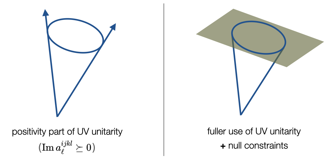
Figure 1: Cartoon view of positivity cone (left) vs capped positivity cone (right). Previous positivity bounds (left) form a convex cone, unbounded away from the vertex, only utilizing the positivity part of the UV unitarity. In this paper, we cap the positivity cone from above (right), using the non-positivity part of the UV unitarity conditions.

We shall first set up the general formalism to bound the $s^{2}$ coefficients of a multi-scalar field theory. The partial wave expansion of a scalar theory can be performed with Legendre polynomials, while that of a general field theory with spin needs Wigner $d$-matrices, which is technically more involved but does not seem to pose any essential obstacle in applying our general method and is left for future work. We will illustrate how to use the method to bound the single scalar theory (see Xu:2023lpq for an application of the upper bound in cosmology) and the theory with two scalars, before applying the method to the Higgs case.

Numerically, we obtain the two-sided bounds by discretizing the dispersive integrals of the sum rules and the null constraints and truncating the UV partial wave expansion at finite angular momentum. This allows us to reduce the procedure to a linear programming (LP) problem with a large number of decision variables, which nevertheless can be solved relatively easily, thanks to the efficiency of modern LP algorithms. For instance, this can be achieved using the built-in command LinearProgramming in mathematica. The numerical efficiency is especially remarkable in the context of a single scalar case. However, in the Higgs case, it does require more computational time due to the increased degrees of freedom, notably the proliferation of decision variables and null constraints. To reduce the running times, we find that we can combine a few sets of spectral densities to significantly reduce the number of decision variables. We plot both 1D (Figure 5) and 2D (Figure 6) bounds for the three Wilson coefficients for the SMEFT Higgs, from which we can see that the new allowed region only occupies a small portion of the Higgs positivity cone.

We may compare the bounds from the capped Higgs positivity cone to the widely used perturbative unitarity bounds. The upper positivity bounds are similar to perturbative unitarity bounds in the sense that they both make use of the unitarity conditions. However, the fundamental difference between the two kinds of bounds are that, while perturbative unitarity bounds rely on the unitarity bounds within the EFT/below the cutoff, the upper positivity bounds originate from the unitarity conditions of the UV theory. We will see that the upper positivity bounds are often stronger than perturbative unitarity bounds, even when the $\sqrt{s}$ is chosen to be close to the EFT cutoff. We also compare the positivity bounds with the experimental constraints on the SMEFT Higgs coefficients, obtained from measurements of Vector Boson Scattering (VBS) at the LHC. We find that the upper positivity bounds are stronger than the experimental limits when the EFT cutoff is greater than $\sim 2$ TeV.

The remainder of the paper is organized as follows. Section 2 introduces and derives the positivity bounds for general multi-field theories, deriving the general null constraints and enumerating the relevant unitarity conditions on the UV partial wave amplitudes beyond positivity. Using examples of the single-scalar and bi-scalar theories, we then establish the LP methodology to obtain new, closed constraints on the coefficients of the associated scattering amplitudes. Section 3 applies the methodology to the effective theory for Higgs scattering amplitudes, leading to the upper bounds on the dimension-8 SMEFT coefficients that “cap” the $s^{2}$ positivity cone. Section 4 compares our theoretical bounds with existing experimental bounds from VBS measurements at the LHC as well as partial wave unitarity constraints of the low energy EFT. Appendix A first presents a pedagogical review of the full partial wave unitarity conditions, and then derives a constraining set of linear unitarity conditions that we use in this paper. In Appendix B, we analytically derive an example upper bound, which helps showcase the inner mechanism of obtaining the upper positivity bounds. Appendix C derives the symmetries of the Higgs amplitudes and connect the amplitude coefficients with the Wilson coefficients. Appendix D presents the details about how to reduce the decision variables in the Higgs case. In Appendix E, we provide more details about how to implement the LP numerically and report on a convergence study of our computational method.

2 Upper bounds in multi-field theories

Recently, positivity bounds have established that, at leading order, certain dimension-8 coefficients of the SMEFT should live in a positivity cone Zhang:2020jyn ; Li:2021lpe . The vertex of the cone corresponds to all of the coefficients being null, and the cone can extend infinitely away from the vertex, admitting arbitrarily large values of the Wilson coefficients. We shall show in this paper that the positivity cone is actually capped from above, as one would expect on general grounds. In the example of SMEFT Higgs operators that we will explicitly work out, the coefficients are confined to a finite, convex region. In this section, we develop a general formalism to obtain upper bounds on the Wilson coefficients in a multi-field theory. We will only consider scattering amplitudes involving scalar fields, which simplifies the partial wave expansion. For fields with spin, the Wigner small-$d$ matrices should be used instead of Legendre polynomials.

We will first present the dispersion relations and introduce the two main ingredients for obtaining the upper positivity bounds. The first are so-called null constraints, a series of integral equations that constrain the partial wave amplitudes, which we will shortly review based on the formulation of Du:2021byy . The second are the UV unitarity bounds away from positivity. The positivity part of the UV unitarity condition gives rise to the aforementioned positivity cone, while the non-positivity part enables us to fully close the allowed region, i.e cap the cone. In Section 2.3, we formulate the problem of obtaining the positivity bounds (both lower and upper) as a linear program treating the partial wave amplitudes as decision variables. As two illustrating examples, in Section 2.4 and 2.5, we apply this method to obtain two-sided bounds for the single scalar theory and the bi-scalar theory.

2.1 Null constraints from crossing symmetry

The null constraints arise when imposing full crossing symmetry Tolley:2020gtv ; Caron-Huot:2020cmc on scattering amplitudes. As we will see, if we start with dispersion relations with only two channels i.e. the sum rules are only $su$ crossing symmetric, then the extra $st$ crossing symmetry needs to be imposed to achieve full crossing symmetry. These null constraints turn out to be very potent in restricting the space of Wilson coefficients, which parallels the situation in the conformal bootstrap where full crossing symmetry is fundamental to its recent success Poland:2018epd . Indeed, without the null constraints, naive use of the partial wave unitarity bounds in the sum rules would not constrain the coefficients from above.

We shall first derive the sum rules from the dispersion relations. Let us consider the amplitude, $A_{ijkl}(s,t)$, for a 2-to-2 scattering process $ij\to kl$ in $D=4$ dimensions, where $i,\,j,\,k,\,l=1,2,...,N$ label different low energy states in an effective theory. For simplicity, we will focus on the massless scalar case with Mandelstam variables satisfying $s+t+u=0$. We work in a self-conjugate basis for the scattering states to simplify the crossing relations, which are given by $A_{ijkl}(s,t)=A_{ikjl}(t,s)$ and $A_{ijkl}(s,t)=A_{ilkj}(u,\,t)$ for $st$ and $su$ crossing respectively. By the (complex) analyticity properties of $A_{ijkl}(s,t)$ in the UV theory, we can use Cauchy’s integral formula along with the Froissart-Martin bound Froissart:1961ux ; Martin:1962rt to relate it to a dispersive integral of its absorptive part, defined by its discontinuity across the real $s$-axis: $\mathrm{Abs}A(s,t)=\frac{1}{2i}\lim_{\epsilon\to 0^{+}}\left[A(s+i\epsilon,t)-A(s-i\epsilon,t)\right]$. In a time reversal invariant theory, which we focus on in this paper, the absorptive part is simply the imaginary part: ${\rm Abs}A_{ijkl}(s,t)={\rm Im}A_{ijkl}(s,t)$. Additionally making use of $su$ symmetry to infer the discontinuity along the negative $s$-axis in terms of the crossed amplitude, $A_{ijkl}(s+i\epsilon,\,t)=A_{ilkj}(-s-i\epsilon-t,\,t)$, one can express $A_{ijkl}$ as Du:2021byy ; deRham:2017avq :

$$A_{ijkl}(s,t) =\frac{\lambda_{ijkl}}{-s}+\frac{\lambda_{ijkl}}{-t}+\frac{\lambda_{ijkl}}{-u}+a^{(0)}_{ijkl}(t)+a^{(1)}_{ijkl}(t)s$$

$$+\int_{\Lambda^{2}}^{\infty}\frac{d\mu}{\pi(\mu+{t\over 2})^{2}}\left[\frac{(s+{t\over 2})^{2}}{\mu-s}\mathrm{Im}\,A_{ijkl}(\mu,\,t)+\frac{(u+{t\over 2})^{2}}{\mu-u}\mathrm{Im}\,A_{ilkj}(\mu,\,t)\right]\,,$$ (1)

where $\lambda_{ijkl}$ are the residues of the poles that are required to be identical by crossing symmetry, and $a^{(0)}_{ijkl}$ and $a^{(1)}_{ijkl}$ are arbitrary functions of $t$ that will be fixed later thanks to $st$ crossing symmetry. $\Lambda$ is the scale associated with the appearance of the lowest modes in the UV theory. It is assumed to be much larger than $s$ and $t$ and can be identified with the cutoff of the EFT. The integration starts from $\Lambda^{2}$ because we have assumed that below $\Lambda^{2}$ the theory is perturbative and the tree level amplitude provides a good approximation. For loop amplitudes, a similar dispersive integral from $\Lambda^{2}$ to infinity can also be obtained by subtracting the low energy part of the dispersive integral deRham:2017imi ; Li:2022aby ; Zhang:2021eeo or equivalently using the arc variables Bellazzini:2020cot , the details of which are deferred for future work.

Eq. (1) is a twice-subtracted dispersion relation for $A_{ijkl}(s,t)$ at fixed $t$, with the arbitrary subtraction point conveniently chosen to at $-{t}/{2}$. Subtracting twice is sufficient to render the terms in the dispersion relations finite, owing to the Froissart-Martin bound. Further subtracting the poles of the amplitude $A_{ijkl}(s,t)$, and defining $v\equiv s+\frac{t}{2}=-u-\frac{t}{2}$ for simplicity yields a dispersion relation for the pole-subtracted amplitude

$$B_{ijkl}(s,t) \equiv A_{ijkl}(s,t)-\frac{\lambda_{ijkl}}{-s}-\frac{\lambda_{ijkl}}{-t}-\frac{\lambda_{ijkl}}{-u}$$ (2)

$$=\tilde{a}^{(0)}_{ijkl}(t)+a^{(1)}_{ijkl}(t)v+\frac{v^{2}}{\pi}\int_{\Lambda^{2}}^{\infty}\!\frac{d\mu}{(\mu+{t\over 2})^{2}}\left[\frac{\mathrm{Im}\,A_{ijkl}(\mu,\,t)}{\mu-v+{t\over 2}}+\frac{\mathrm{Im}\,A_{ilkj}(\mu,\,t)}{\mu+v-{t\over 2}}\right]\,,$$

where we have also introduced $\tilde{a}^{(0)}_{ijkl}(t)=a^{(0)}_{ijkl}(t)+a^{(1)}_{ijkl}(t){t\over 2}$. Since we will be interested in studying the low energy limit of the amplitude modelled by an EFT, we expand $B_{ijkl}$ on the left hand side in terms of small $s$ and $t$,

$$B_{ijkl}(s,t) =\sum_{n\geq 0}c_{ijkl}^{0,n}t^{n}+\sum_{n\geq 0}c_{ijkl}^{1,n}vt^{n}+\sum_{m\geq 2}\sum_{n\geq 0}c_{ijkl}^{m,n}v^{m}t^{n}\,.$$ (3)

While $c_{ijkl}^{0,n}$ and $c_{ijkl}^{1,n}$ correspond to the expansion coefficients of the soon-to-be determined $\tilde{a}^{(0)}_{ijkl}(t)$ and $a^{(1)}_{ijkl}(t)$, matching the expansions on both sides of Eq. (2) for $m\geq 2$ leads to a set of sum rules for the Wilson coefficients

$$c_{ijkl}^{m,n} =\Bigg{\langle}\big{[}\rho_{\ell}^{ijkl}(\mu)+(-1)^{m}\rho_{\ell}^{ilkj}(\mu)\big{]}\sum_{p=0}^{n}\frac{L_{\ell}^{p}H_{m+1}^{n-p}}{\mu^{m+n+1}}\Bigg{\rangle}\,,~{}~{}~{}~{}m\geq 2.$$ (4)

Here we have used the partial wave expansion for the absorptive part of the amplitude at energy scale $\sqrt{\mu}$,

$$\mathrm{Im}\,A_{ijkl}(\mu,\,t)=16\pi\sum_{\ell=0}^{\infty}(2\ell+1)P_{\ell}\left(1+\frac{2t}{\mu}\right)\rho_{\ell}^{ijkl}(\mu)\,,$$ (5)

with $P_{\ell}$ being the Legendre polynomial and the “spectral density” defined as

$$\rho^{ijkl}_{\ell}(\mu)\equiv\mathrm{Im}\,a_{\ell}^{ijkl}(\mu)\,,$$ (6)

and we have introduced shorthand notations

$$~{}~{}~{}~{}~{}~{}~{}~{}~{}~{}~{}~{}\Big{\langle}\,...\,\Big{\rangle}\equiv\sum_{\ell}16(2\ell+1)\int_{\Lambda^{2}}^{\infty}d\mu\Big{(}\,...\,\Big{)},$$ (7)

$$L_{\ell}^{n} \equiv\frac{\Gamma(\ell+n+1)}{n!\Gamma(\ell-n+1)\Gamma(n+1)},~{}~{}H_{m+1}^{q}\equiv\frac{\Gamma(m+q+1)}{(-2)^{q}\Gamma(q+1)\Gamma(m+1)}.$$ (8)

The sum rules will be the central objects we will use to extract the bounds on the Wilson coefficients.

Due to the crossing symmetry of the amplitude, the $c_{ijkl}^{m,n}$ must satisfy certain relations among themselves, called null constraints Du:2021byy ; Tolley:2020gtv ; Caron-Huot:2020cmc . Since the dispersion relation (2)/sum rules (4), and thus $c_{ijkl}^{m\geq 2,n}$ themselves are already $su$ symmetric, we only need to impose $st$ crossing symmetry on the amplitude $B_{ijkl}(s,t)=B_{ikjl}(t,s)$ to achieve full crossing symmetry. This leads to a series of identities relating coefficients $c_{ijkl}^{m,n}$ with a common $m+n$:

$$n_{ijkl}^{p,q} =\sum_{a=p}^{p+q}\frac{\Gamma(a+1)c_{ijkl}^{a,p+q-a}}{2^{a-p}\Gamma(p+1)\Gamma(a-p+1)}-\sum_{b=q}^{p+q}\frac{\Gamma(b+1)c_{ikjl}^{b,p+q-b}}{2^{b-q}\Gamma(q+1)\Gamma(b-q+1)}=0\,.$$ (9)

For a fixed order $p+q={f}$, there are $f+1$ identities (given by choosing $p=0,1,...,f$), in which $c_{ijkl}^{0,p+q}$, $c_{ijkl}^{1,p+q-1}$, $c_{ikjl}^{0,p+q}$ and $c_{ikjl}^{1,p+q-1}$ are not useful to us since they do not have a dispersive integral representation like Eq. (4). We therefore eliminate them by first using four of the identities to solve for them as linear sums of $c_{ijkl}^{m\geq 2,n}$ and then plugging the solution into the $f-3$ remaining identities. One additional set of relations between $c_{ijkl}^{1,n}$ can be obtained by applying $su$ crossing symmetry on the amplitude, $B_{ijkl}(s,t)=B_{ilkj}(u,t)$. The fact that $s\leftrightarrow u$ corresponds to $v\to-v$ implies:

$$\evaluated{c_{ijkl}^{1,n}+c_{ilkj}^{1,n}}_{c^{1,n}\rightarrow c^{m\geq 2,n^{\prime}}}=0\,,$$ (10)

in which we again substitute $c^{1,n}$ with $c^{m\geq 2,n^{\prime}}$ using the solution we just obtained. We are then left with $f-2$ null constraints, which involve only $c_{ijkl}^{m,n}$, $c_{ikjl}^{m,n}$ and $c_{ilkj}^{m,n}$ with $m\geq 2$ and $m+n=f$. The rest of the $c_{ijkl}^{m\geq 2,n}$ terms in the expansion of Eq. (4) are $su$ invariant by construction, leaving Eqs. (9) and (10) as the full set of null constraints implied by crossing symmetry. For example, the first set of nontrivial null constraints starts at $m+n=f=4$. (see Du:2021byy for the higher order results), and they are

$$\begin{split}c_{{ijkl}}^{{2,2}}-c_{{ikjl}}^{{2,2}}+\frac{3c_{{ijkl}}^{{3,1}}}{2}-\frac{3c_{{ikjl}}^{{3,1}}}{2}+\frac{3c_{{ijkl}}^{{4,0}}}{2}-\frac{3c_{{ikjl}}^{{4,0}}}{2}=0\,,\\ -c_{{ikjl}}^{{2,2}}-c_{{iklj}}^{{2,2}}+\frac{3c_{{ijkl}}^{{3,1}}}{4}-\frac{c_{{ikjl}}^{{3,1}}}{2}-\frac{c_{{iklj}}^{{3,1}}}{2}+\frac{3c_{{ilkj}}^{{3,1}}}{4}+c_{{ijkl}}^{{4,0}}+\frac{c_{{ikjl}}^{{4,0}}}{2}+\frac{c_{{iklj}}^{{4,0}}}{2}+c_{{ilkj}}^{{4,0}}=0\,,\end{split}$$ (11)

obtained from $n^{2,2}_{ijkl}$ and Eq. (10) with $n=3$. One possible way forward is to simply slice out the $c_{{ijkl}}^{m,n}$ coefficient space with the above null constraints, assuming one can extract positivity bounds for sufficiently many $c_{{ijkl}}^{m,n}$ coefficients directly from the sum rules (4), via the mathematical moment approach Arkani-Hamed:2020blm ; Bellazzini:2020cot ; Chiang:2021ziz , for example. These $c_{{ijkl}}^{m,n}$ null constraints simply mean that the independent $c_{{ijkl}}^{m,n}$ coefficients live in a linear subspace of the full $c_{{ijkl}}^{m,n}$ space. However, a more efficient use of the null constraints is, as we shall see shortly, to turn them into a set of identities for the UV partial wave amplitudes, which makes the name of null constraints more justified. Then, we will find that these reformulated null constraints can be used to facilitate the extraction of positivity bounds for the coefficients, very efficiently for the first few orders.

Concretely, substituting the sum rules (4) into the null constraints (9-10), we get a set of constraints on $\rho_{\ell}^{ijkl}$ that take the following general form:

$$\sum_{\ell}16(2\ell+1)\int_{\Lambda^{2}}^{\infty}\frac{\differential\mu}{\mu^{r+4}}\Bigg{[}C_{r,i_{r}}(\ell)\rho_{\ell}^{{ijkl}}(\mu)+D_{r,i_{r}}(\ell)\rho_{\ell}^{{ijlk}}(\mu)+E_{r,i_{r}}(\ell)\rho_{\ell}^{{ikjl}}(\mu)$$

$$\hskip 100.00015pt+F_{r,i_{r}}(\ell)\rho_{\ell}^{{iklj}}(\mu)+G_{r,i_{r}}(\ell)\rho_{\ell}^{{iljk}}(\mu)+H_{r,i_{r}}(\ell)\rho_{\ell}^{{ilkj}}(\mu)\Bigg{]}=0\,,$$ (12)

where $r\equiv f-3=1,2,...$ is the order of null constraints, which corresponds to $p+q-3$ in Eq. (9) or $n-2$ in Eq. (10). At the $r$-th order, there are $r+1$ independent constraints for generic $i,j,k,l$, labelled by $i_{r}=1,...,r+1$. $C_{r,i_{r}}(\ell),D_{r,i_{r}}(\ell),...,H_{r,i_{r}}(\ell)$ are polynomials in $\ell$ of degree $\leq 2r+2$. For the lowest order constraints given as an example in Eq (11), we have:

$$\begin{aligned} C_{1,1}(\ell)&=\frac{\ell^{4}}{4}+\frac{\ell^{3}}{2}-\frac{\ell^{2}}{4}-\frac{\ell}{2},&C_{1,2}(\ell)&=2,\\ D_{1,1}(\ell)&=0,&D_{1,2}(\ell)&=-\frac{\ell^{4}}{4}-\frac{\ell^{3}}{2}+\frac{9\ell^{2}}{4}+\frac{5\ell}{2}-2,\\ E_{1,1}(\ell)&=-C_{1,1}(\ell),&E_{1,2}(\ell)&=-\frac{\ell^{4}}{4}-\frac{\ell^{3}}{2}+\frac{5\ell^{2}}{4}+\frac{3\ell}{2},\\ F_{1,1}(\ell)&=0,&F_{1,2}(\ell)&=E_{1,2}(\ell),\\ G_{1,1}(\ell)&=-\frac{\ell^{4}}{4}-\frac{\ell^{3}}{2}+\frac{13\ell^{2}}{4}+\frac{7\ell}{2}-6,\phantom{-}&G_{1,2}(\ell)&=D_{1,2}(\ell),\\ H_{1,1}(\ell)&=-G_{1,1}(\ell),&H_{1,2}(\ell)&=2\,.\end{aligned}$$ (13)

For a specific choice of $i,j,k,l$, permuting $j,k,l$ can lead to extra constraints. On the other hand, additional degeneracies may exist, which reduces the number of independent ones. For example, if we choose $i,j,k,l$ to be $1,2,3,4$, in addition to the null constraint obtained by setting $i=1,j=2,k=3,l=4$ in Eq. (12) in a form of

$$\sum\int\cdots\Big{[}C\rho_{\ell}^{{1234}}+D\rho_{\ell}^{{1243}}+E\rho_{\ell}^{{1324}}+F\rho_{\ell}^{{1342}}+G\rho_{\ell}^{{1423}}+H\rho_{\ell}^{{1432}}\Big{]}=0\,,$$

we can also set $j,k,l$ to be other combinations of $2,3,4$ to obtain more null constraints relating $\rho_{\ell}^{{1234}},\rho_{\ell}^{{1324}},...$, such as

$$\sum\int\cdots\Big{[}C\rho_{\ell}^{{1324}}+D\rho_{\ell}^{{1342}}+E\rho_{\ell}^{{1234}}+F\rho_{\ell}^{{1243}}+G\rho_{\ell}^{{1432}}+H\rho_{\ell}^{{1423}}\Big{]}=0\,,$$

among several others. When deriving the null constraints for bi-scalar and four scalars, we need to exhaust all the permutations in Eq. (9-10) to get the full set of null constraints.

We stress that the $\rho^{ijkl}_{\ell}(\mu)$’s are unknown in general, since they can only be determined in terms of the scattering amplitudes of the UV theory – note that in the dispersive integrals $\mu$ goes from $\Lambda^{2}$ to infinity. Nevertheless, we have shown here that they respect a series of null constraints that we will use later to bound the coefficients of the low energy EFT. These null constraints imply that the contributions from higher spin-$\ell$ components of $\rho^{ijkl}_{\ell}(\mu)$ are generally highly suppressed, which makes them very efficient at closing in the parameter space of the EFT coefficients. For the particular case of the $s^{2}$ coefficients, as we will see, they allow us to impose upper bounds on the Wilson coefficients from the sum rules, in conjunction with the upper bounds of the partial wave amplitudes from the unitarity in the UV.

Apart from these null constraints, crossing symmetry also implies symmetries among the spectral densities $\rho^{ijkl}_{\ell}$ when swapping their initial or final indices. To see this, note that the $tu$ crossing symmetry $A_{ijkl}(\mu,t)=A_{jikl}(\mu,u)=A_{ijlk}(\mu,u)$ implies that $a_{\ell}^{ijkl}(\mu)=(-1)^{\ell}a_{\ell}^{jikl}(\mu)=(-1)^{\ell}a_{\ell}^{ijlk}(\mu)$. This is due to the property of the Legendre polynomials $P_{\ell}(-z)=(-1)^{\ell}P_{\ell}(z)$, which leads to

$$A_{jikl}(\mu,u) =16\pi\sum_{\ell=0}^{\infty}\quantity(2\ell+1)P_{\ell}\left(1+\frac{2u}{\mu}\right)a_{\ell}^{jikl}(\mu)$$ (14)

$$=16\pi\sum_{\ell=0}^{\infty}\quantity(2\ell+1)(-1)^{\ell}P_{\ell}\left(1+\frac{2t}{\mu}\right)a_{\ell}^{jikl}(\mu)\,,$$ (15)

$$A_{ijkl}(\mu,t) =16\pi\sum_{\ell=0}^{\infty}\quantity(2\ell+1)P_{\ell}\left(1+\frac{2t}{\mu}\right)a_{\ell}^{ijkl}(\mu)\,,$$ (16)

and the corresponding relations

$$\rho^{ijkl}_{\ell}=(-1)^{\ell}\rho^{jikl}_{\ell}=(-1)^{\ell}\rho^{ijlk}_{\ell}\,.$$ (17)

In the following examples involving a single scalar, two scalars and the Higgs multiplet, we will use the identities implicitly to eliminate a number of variables. For example, they imply that $\rho^{1111}_{\ell}=\rho^{1122}_{\ell}=0$ for odd $\ell$.

2.2 Unitarity conditions from the UV

In order to obtain positivity bounds, we also need some inequality conditions on the spectral densities $\rho^{ijkl}_{\ell}(\mu)={\rm Im}a_{\ell}^{ijkl}(\mu)$ from partial wave unitarity of the UV theory. These conditions lie at the heart of the positivity bounds, which in essence are just the projected-down version of these UV conditions on the IR theory by analyticity. Previous positivity bounds on the SMEFT only utilized the positivity part of these conditions, and now we shall also make use of the non-positivity parts. We will not use the full nonlinear unitarity, but restrict ourselves to the linear conditions, which are easily implemented in the linear programs and are sufficiently strong to close the Higgs positivity cone. In this subsection, we will briefly illustrate how to obtain a couple of these conditions, before listing all of the results we will use in the linear programs, deferring the details of the full derivations to Appendix A.

Recall that, for the generic process $ij\to kl$, partial wave unitarity can be written as (see Appendix A)

$$\mathrm{Im}a_{\ell}^{ijkl}=\sum_{mn}\,\eta_{mn}a_{\ell}^{ijmn}\quantity(a_{\ell}^{klmn})^{*}+\sum_{X\neq mn}a_{\ell}^{ij\rightarrow X}\quantity(a_{\ell}^{kl\rightarrow X})^{*}\,,$$ (18)

where $a_{\ell}^{ij\rightarrow X}$ is the partial wave amplitude for the state $ij$ into some intermediate state $X$ and the phase space factor $\eta_{mn}=1/2$ if $m=n$ and $\eta_{mn}=1$ if $m\neq n$. The positivity part of the unitarity conditions refers to the fact that Eq. (18) implies that $\mathrm{Im}a_{\ell}^{ijkl}$ is a positive semi-definite matrix, viewing $ij$ and $kl$ as the two indices of the matrix. This allows one to obtain a set of positivity bounds via semi-definite programming Li:2021lpe ; Du:2021byy . The bounds extracted by this semi-definite programming method are optimal insofar as they only include the positivity part of partial wave unitarity. These “true” positivity bounds carve out a convex cone in the coefficient space, starting from its vertex and extending away to infinity. Thus, the “true” positivity bounds can be regarded as providing the “lower bounds” for the $s^{2}$ coefficients. In this paper, we will go beyond that by using the non-positivity parts of partial wave unitarity, which allow us to find upper bounds for all of the examples considered in this paper, capping all of the $s^{2}$ coefficients from above.

Using simple inequality relaxation and Eq. (17), we can derive from Eq. (18) the following two-sided constraints for the imaginary parts of the partial waves (see Appendix A):

$$0\leq\mathrm{Im}a_{\ell}^{iiii}\leq 2,~{}~{}~{}~{}0\leq\mathrm{Im}a_{\ell}^{ijij}\leq\frac{1}{2},~{}~{}~{}~{}i\neq j.~{}$$ (19)

For example, to derive the first inequality above, we can consider the process $ii\to ii$. For this process, the terms on the right hand side of (18) are all positive, so picking out only $X=ii$ for the intermediate states gives

$$\mathrm{Im}a_{\ell}^{iiii}\geq\frac{1}{2}|a_{\ell}^{iiii}|^{2}=\frac{1}{2}\left(\mathrm{Im}a_{\ell}^{iiii}\right)^{2}+\frac{1}{2}\left(\mathrm{Re}a_{\ell}^{iiii}\right)^{2}~{}~{}~{}\Rightarrow~{}~{}~{}0\leq\mathrm{Im}a_{\ell}^{iiii}\leq 2.$$ (20)

Similarly, as shown in Appendix A, we can also derive two-sided conditions for the inelastic partial waves $\mathrm{Im}a_{\ell}^{iijj}$ and $\mathrm{Im}a_{\ell}^{ijkl}$ ($i\neq j\neq k\neq l$): $-1\leq\mathrm{Im}a_{\ell}^{iijj}\leq 1,~{}-\frac{1}{4}\leq\mathrm{Im}a_{\ell}^{ijkl}\leq\frac{1}{4}$. We see that, in contrast to those of $\mathrm{Im}a_{\ell}^{iiii}$ and $\mathrm{Im}a_{\ell}^{ijij}$, they are not positive semi-definite.

We can actually get stronger conditions on these two coefficients. To see this, let us denote $\mathcal{X}^{ij,kl}$ as the set of all intermediate states that contribute to the scattering process $ij\rightarrow X\rightarrow kl$, and we must have $\mathcal{X}^{ij,kl}\subseteq\mathcal{X}^{ij,ij}\cap\mathcal{X}^{kl,kl}$. This leads to

$$\left|\mathrm{Im}a^{ijkl}_{\ell}\right|^{2} =\left|\sum_{X\in\mathcal{X}^{ij,kl}}a_{\ell}^{ij\to X}\left(a_{\ell}^{kl\to X}\right)^{*}\right|^{2}$$

$$\leq\sum_{X\in\mathcal{X}^{ij,kl}}\quantity|a_{\ell}^{ij\to X}|^{2}\sum_{X\in\mathcal{X}^{ij,kl}}\quantity|a_{\ell}^{kl\to X}|^{2}\leq\sum_{X\in\mathcal{X}^{ij,ij}}\quantity|a_{\ell}^{ij\to X}|^{2}\sum_{X\in\mathcal{X}^{kl,kl}}\quantity|a_{\ell}^{kl\to X}|^{2}$$

$$=\mathrm{Im}a^{ijij}_{\ell}\mathrm{Im}a^{klkl}_{\ell}\leq\left(\frac{\mathrm{Im}a^{ijij}_{\ell}+\mathrm{Im}a^{klkl}_{\ell}}{2}\right)^{2}\,,$$ (21)

where the first inequality arises from the Cauchy-Schwarz inequality and the second is due to the fact that the sets $\mathcal{X}^{ij,ij}$ and $\mathcal{X}^{kl,kl}$ are both larger than their intersection, $\mathcal{X}^{ij,kl}$. Taking the square root of the above inequality and recognizing that $\mathrm{Im}a^{ijij}_{\ell}\geq 0$, we obtain

$$\big{|}\mathrm{Im}a^{ijkl}_{\ell}\big{|}\leq\frac{\mathrm{Im}a^{ijij}_{\ell}+\mathrm{Im}a^{klkl}_{\ell}}{2},~{}~{}~{}~{}~{}\forall~{}i,j,k,l$$ (22)

This condition turns out to be pivotal to cap the Higgs positivity cone. Again using the Cauchy-Schwarz inequality plus some re-arrangements of the partial wave unitarity conditions, as shown in Appendix A, we can also derive

$$\big{|}\mathrm{Im}a_{\ell}^{ijkl}\big{|}\leq\frac{1}{2}-\frac{\mathrm{Im}a_{\ell}^{ijij}+\mathrm{Im}a_{\ell}^{klkl}}{2},~{}~{}~{}~{}\big{|}\mathrm{Im}a_{\ell}^{iijj}\big{|}\leq 2-\frac{\mathrm{Im}a^{iiii}_{\ell}+\mathrm{Im}a^{jjjj}_{\ell}}{2}\,,$$ (23)

$$\big{|}(\mathrm{Im}a^{iijj}_{\ell}+\mathrm{Im}a^{kkll}_{\ell})\pm(\mathrm{Im}a^{iikk}_{\ell}+\mathrm{Im}a^{jjll}_{\ell})\big{|}\leq 2\,,$$ (24)

where $i\neq j\neq k\neq l$. The first two conditions can be combined with inequality (22) to become

$$\big{|}\mathrm{Im}a_{\ell}^{iijj}\big{|}\leq 1-\Big{|}1-\frac{\mathrm{Im}a_{\ell}^{iiii}+\mathrm{Im}a_{\ell}^{jjjj}}{2}\Big{|},~{}~{}~{}~{}\big{|}\mathrm{Im}a_{\ell}^{ijkl}\big{|}\leq\frac{1}{4}-\Big{|}\frac{1}{4}-\frac{\mathrm{Im}a_{\ell}^{ijij}+\mathrm{Im}a_{\ell}^{klkl}}{2}\Big{|}.$$ (25)

In summary, we will use the following linear unitarity conditions in the linear programs to constrain the $s^{2}$ coefficients in the multi-field theory, written in terms of the spectral densities $\rho^{ijkl}_{\ell}={\rm Im}a_{\ell}^{ijkl}$,

$$0\leq\rho_{\ell}^{iiii}\leq 2,\quad\hskip 2.79999pt\big{|}\rho_{\ell}^{iijj}\big{|}\leq 1-\Big{|}1-\frac{\rho_{\ell}^{iiii}+\rho_{\ell}^{jjjj}}{2}\Big{|},\,$$

$$0\leq\rho_{\ell}^{ijij}\leq\frac{1}{2},\quad\big{|}\rho_{\ell}^{ijkl}\big{|}\leq\frac{1}{4}-\Big{|}\frac{1}{4}-\frac{\rho_{\ell}^{ijij}+\rho_{\ell}^{klkl}}{2}\Big{|},~{}~{}~{}~{}~{}(i\neq j\neq k\neq l)$$ (26)

$$\big{|}(\rho^{iijj}_{\ell}+\rho^{kkll}_{\ell})\pm(\rho^{iikk}_{\ell}+\rho^{jjll}_{\ell})\big{|}\leq 2.$$

2.3 Constraining Wilson coefficients

We will now combine the previous ingredients to constrain the Wilson coefficients in a multi-field EFT. For phenomenologists, the $s^{2}$ coefficients in the tree-level scattering amplitudes, $c_{ijkl}^{2,0}={\rm d}^{2}A_{ijkl}(s,t)/(2{\rm d}s^{2})$, are of greatest interest, as they correspond to a linear combination of dimension-8 Wilson coefficients (and quadratic terms of dimension-6 coefficients). These are the leading coefficients in the EFT expansion of the amplitudes for which positivity bounds can be obtained. Although we will focus on bounding only the $c_{ijkl}^{2,0}$ coefficients in this paper, we stress that the sum rules along with the null constraints and the UV unitarity conditions we have obtained can be used to constrain all of the Wilson coefficients. The positivity part of partial wave unitarity can be fully implemented to constrain the $c_{ijkl}^{2,0}$ coefficients via either the convex cone Zhang:2020jyn or the semi-definite program approach Li:2021lpe . In this subsection we will formulate the problem of finding the upper bounds of the $c_{ijkl}^{2,0}$ coefficients as a LP in a generic form.

Essentially, our strategy is to numerically find the upper bounds via the sum rules by brute force. This is made possible thanks to the unitarity conditions and the null constraints. To this end, we first change the integration variable from $\mu$ to $z={\Lambda^{2}}/{\mu}$, and discretize the $z$ variable as ${n}/{N}$ with $n=1,2,...,N$ Chiang:2022jep , approximating $\int_{0}^{1}\differential z$ with $\sum_{n=1}^{N}\frac{1}{N}$. We can also impose a cutoff $\ell_{M}$ on the sum over the UV spin $\ell$, since the null constraints require the higher spin spectral densities $\rho_{\ell}^{ijkl}$ to be highly suppressed (see Appendix B). Numerically, we can indeed confirm that the results converge with $\ell_{M}$ (see Appendix E). Thus, the $c_{ijkl}^{2,0}$ sum rules become

$$c_{ijkl}^{2,0} =\sum_{\ell}(2\ell+1)\int_{\Lambda^{2}}^{\infty}\frac{\differential\mu}{\mu^{3}}16(\rho_{\ell}^{{ijkl}}(\mu)+\rho_{\ell}^{{ilkj}}(\mu))$$ (27)

$$~{}~{}~{}~{}~{}~{}\Rightarrow~{}~{}c^{2,0}_{ijkl}\approx\frac{1}{\Lambda^{4}}\sum\limits_{\ell=0}^{\ell_{M}}(2\ell+1)\sum\limits_{n=1}^{N}\frac{1}{N}\frac{n}{N}16\left(\rho_{\ell,n}^{ijkl}+\rho_{\ell,n}^{ilkj}\right),$$ (28)

and the null constraints are similarly discretized . Thus, $c_{ijkl}^{2,0}$ becomes a linear combination of many unknown variables $\rho^{ijkl}_{\ell,n}\equiv\rho^{ijkl}_{\ell}({\Lambda^{2}N}/{n})$, subject to a set of linear inequality and equality constraints. Maximizing $\sum_{ijkl}\alpha^{ijkl}c^{2,0}_{ijkl}$ over all possible variables $\rho^{ijkl}_{\ell,n}$ is a well defined LP problem, where $\alpha^{ijkl}$ are constants specifying which direction to optimize in the parameter space furnished by all $c^{2,0}_{ijkl}$ . More explicitly, the programming task can be summarised as follows:

$$\mathbf{Decision~{}variables}$$

$$\hskip 10.00002pt\rho_{\ell,n}^{ijkl},~{}~{}~{}\ell=0,...,\ell_{M},~{}~{}~{}n=1,2,...,N,~{}~{}~{}(\forall\ i,j,k,l)$$ (29)

$$\mathbf{Maximize}$$

$$\hskip 11.99998pt\sum_{ijkl}\alpha^{ijkl}c^{2,0}_{ijkl},~{}~{}~{}{\rm where}~{}~{}c^{2,0}_{ijkl}=\frac{1}{\Lambda^{4}}\sum\limits_{\ell=0}^{\ell_{M}}(2\ell+1)\sum\limits_{n=1}^{N}\frac{1}{N}\frac{n}{N}16\left(\rho_{\ell,n}^{ijkl}+\rho_{\ell,n}^{ilkj}\right)\,,$$ (30)

$$\mathbf{Subject\ to}$$

$$\hskip 1.99997pt\left.\begin{array}[]{lr}0\leq\rho_{\ell,n}^{iiii}\leq 2,\hskip 6.00006pt\big{|}\rho_{\ell,n}^{iijj}\big{|}\leq 1-\Big{|}1-\frac{\rho_{\ell,n}^{iiii}+\rho_{\ell,n}^{jjjj}}{2}\Big{|}\\[8.53581pt] 0\leq\rho_{\ell,n}^{ijij}\leq\frac{1}{2},~{}\big{|}\rho_{\ell,n}^{ijkl}\big{|}\leq\frac{1}{4}-\Big{|}\frac{1}{4}-\frac{\rho_{\ell,n}^{ijij}+\rho_{\ell,n}^{klkl}}{2}\Big{|}\\[11.38109pt] \big{|}(\rho^{iijj}_{\ell,n}+\rho^{kkll}_{\ell,n})\pm(\rho^{iikk}_{\ell,n}+\rho^{jjll}_{\ell,n})\big{|}\leq 2\end{array}\right\}~{}~{}(i\neq j\neq k\neq l);$$ (34)

$$~{}~{}\rho^{ijkl}_{\ell,n}=(-1)^{\ell}\rho^{jikl}_{\ell,n}=(-1)^{\ell}\rho^{ijlk}_{\ell,n},\hskip 65.00009pt(\forall\ i,j,k,l);$$

$$~{}~{}\sum\limits_{\ell=0}^{\ell_{M}}(2\ell+1)\sum\limits_{n=1}^{N}\frac{1}{N}\left(\frac{n}{N}\right)^{r+2}\Bigg{[}C_{r,i_{r}}(\ell)\rho_{\ell,n}^{{ijkl}}+D_{r,i_{r}}(\ell)\rho_{\ell,n}^{{ijlk}}+E_{r,i_{r}}(\ell)\rho_{\ell,n}^{{ikjl}}$$

$$\hskip 140.00021pt+F_{r,i_{r}}(\ell)\rho_{\ell,n}^{{iklj}}+G_{r,i_{r}}(\ell)\rho_{\ell,n}^{{iljk}}+H_{r,i_{r}}(\ell)\rho_{\ell,n}^{{ilkj}}\Bigg{]}=0\,,$$ (35)

Sometimes, the numerical results will converge faster if we also include a much larger partial wave, which will be labelled as $\ell_{\infty}$. In the next subsections, we will work through two example theories of a single scalar or a pair of scalars, illustrating how we perform the LP in detail.

The constraints listed in (35) are generic ones. For a specific model, the symmetries of the theory can give rise to additional constraints, such as extra relations among the amplitude coefficients, that can also be implemented in the LP. They can act similarly to the null constraints in constraining the parameter space, reducing the number of decision variables by relating different $\rho_{\ell,n}^{ijkl}$.

We would like to emphasise here that positivity bounds are a unique, UV probe of the allowed space of IR Wilson coefficients. For a Lagrangian of dimension-8 operators of the form

$$\mathcal{L}_{\mathrm{dim-8}}=\sum_{I}C_{I}^{(8)}\mathcal{O}_{I}^{(8)}=\sum_{I}\frac{\bar{C}_{I}^{(8)}}{\Lambda_{\mathrm{{}_{EFT}}}^{4}}\mathcal{O}_{I}^{(8)}\,,$$ (36)

the $s^{2}$ amplitude coefficients, i.e., our objective functions $c^{2,0}_{ijkl}$, are simple combinations of $C_{I}^{(8)}$’s. $C_{I}^{(8)}$ therefore acquires a bound of the form $C_{I}^{(8)}\leq a/\Lambda^{4}$ via Eq. (30), where $a$ is a dimensionless number, and the dimensionless coefficient $\bar{C}_{I}^{(8)}$ is bounded by $C_{I}^{(8)}\leq a(\Lambda_{\mathrm{{}_{EFT}}}/\Lambda)^{4}$. If we identify the cutoff scale of EFT $\Lambda_{\mathrm{{}_{EFT}}}$ with our lower limit of integration $\Lambda$ in the dispersion relation, which is always true if we assume perturbativity of the UV theory below $\Lambda_{\mathrm{{}_{EFT}}}$ (see Eq. (1) and the discussion below it), then our result directly bounds the dimensionless $\bar{C}_{I}^{(8)}$ through $\bar{C}_{I}^{(8)}\leq a$ with no dependence on $\Lambda_{\rm EFT}$ or any scale. This is in contrast to other bounds that might be obtained from experiments or partial wave unitarity in the low energy EFT which clearly suffer from a degeneracy due to the lack of knowledge on both $\bar{C}_{I}^{(8)}$ and $\Lambda_{\mathrm{{}_{EFT}}}$. The former sets limits on the combination $\bar{C}_{I}^{(8)}/\Lambda_{\mathrm{{}_{EFT}}}^{4}\sim c^{2,0}_{ijkl}$, while the latter constrains $\bar{C}_{I}^{(8)}s^{2}/\Lambda_{\mathrm{{}_{EFT}}}^{4}\sim s^{2}c^{2,0}_{ijkl}$, meaning that certain theoretical assumptions are always required to make statements about the couplings or mass scale of the associated UV theory. Being able to bound $\bar{C}_{I}^{(8)}$ directly is therefore highly complementary to the information obtained from the other bounds, as we discuss in Section 4 for the case of Higgs operators in the SMEFT.

2.4 Example: single scalar

We start with the simplest case where the low energy theory includes a single massless, real scalar. As is well known, the associated EFT has a single independent operator at dimension-8, whose Wilson coefficient maps to $c^{2,0}$ at tree-level:

$$\mathcal{L}^{(8)}=\frac{g_{2}}{2}(\partial^{\mu}\phi\partial_{\mu}\phi)^{2}\,\quad\Rightarrow\quad c^{2,0}=2g_{2}.$$ (37)

It reduces the generic scattering situation to $i=j=k=l$ and we therefore omit those indices. Also, as a result of Eq. (17), the spectral density $\rho_{\ell,n}$ vanishes for odd $\ell$. Since the $c^{2,0}$ coefficient is a positive sum of spectral densities which are themselves positive for the single scalar case, the lower bound is trivially zero and corresponds to the “first” positivity bound: $c^{2,0}\geq 0$.

To get an upper bound on $c^{2,0}$, we exploit the LP proposed in the last subsection, which in this case reads

$$\mathbf{Decision~{}variables}$$

$$\hskip 11.99998pt\rho_{\ell,n}$$

$$\mathbf{Maximize}$$

$$\hskip 11.99998ptc^{2,0}=\frac{1}{\Lambda^{4}}\sum\limits_{\ell=0,2,...,\ell_{M};\ell_{\infty}}(2\ell+1)\sum\limits_{n=1}^{N}\frac{1}{N}\frac{n}{N}32\rho_{\ell,n}\,,$$ (38)

$$\mathbf{Subject\,to}$$

$$\hskip 11.99998pt0\leq\rho_{\ell,n}\leq 2\,,$$ (39)

$$\hskip 11.99998pt\sum\limits_{\ell=0,2,...,\ell_{M};\ell_{\infty}}(2\ell+1)\sum\limits_{n=1}^{N}\frac{1}{N}\left(\frac{n}{N}\right)^{r+2}C^{1111}_{r,i_{r}}(\ell)\rho_{\ell,n}=0\,,$$ (40)

where $C^{1111}_{r,i_{r}}$ represents certain linear combinations of the corresponding $C(\ell),D(\ell),...,H(\ell)$ in Eq. (12) when $i=j=k=l$, which are polynomials in $\ell$ of degree $\leq 2r+2$. In this case, we observe there to be $\lfloor(r-1)/3\rfloor+1$ null constraints at the $r$-th order, where $\lfloor x\rfloor$ denotes the floor integer function. Explicitly, at the first three orders, for example, we have

$$C^{1111}_{1,1} =\ell^{4}+2\ell^{3}-7\ell^{2}-8\ell\,,$$ (41)

$$C^{1111}_{2,1} =\ell^{6}+3\ell^{5}-\frac{37}{2}\ell^{4}-42\ell^{3}+\frac{107}{2}\ell^{2}+75\ell\,,$$ (42)

$$C^{1111}_{3,1} =\ell^{8}+4\ell^{7}-38\ell^{6}-128\ell^{5}+457\ell^{4}+1132\ell^{3}-1860\ell^{2}-2448\ell\,.$$ (43)

To evaluate this LP problem, we set a cutoff $\ell_{M}=100$ for the sum over the partial waves. However, we also generally include a very large partial wave term, $\ell_{\infty}$, to improve the numerical convergence; here we have chosen $\ell_{\infty}=10000$. The optimisation has ${\cal O}(\ell_{M}/2)\times N$ decision variables $\rho_{\ell,n}$ (recall that in this case $\rho_{\ell=\mathrm{odd},n}=0$), each subject to a unitarity bound and additionally constrained by the set of null constraints up to a given order, $r$.

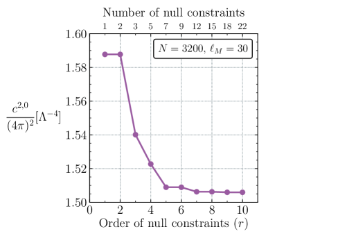
Figure 2: Upper bound on the amplitude coefficient for the single real scalar theory, $c^{2,0}$, in units of $(4\pi)^{2}$ and $\Lambda^{-4}$ resulting from our optimisation procedure as a function of the order of null constraints applied. The upper $x$-axis labels count the number of independent null constraints appearing up to each order.

The result is shown in Figure 2, which plots the upper bound on $c^{2,0}$ in units of $(4\pi)^{2}$ and $\Lambda^{-4}$ as a function of the order of null constraints applied. $N=3200$ points are used for the discretized integral, which is observed to yield a solid convergence as $N$ increases (See Appendix E). We can see that the result converges quickly upon applying higher and higher orders of null constraints, and conclude that the $s^{2}$ coefficient $c^{2,0}$ is bounded both from above and below:

$$0\leq\frac{c^{2,0}}{(4\pi)^{2}}\leq\frac{1.506}{\Lambda^{4}}.$$ (44)

Note that the units of $(4\pi)^{2}$ are consistent with naive dimensional analysis Manohar:2018aog . The upper bound on $c^{2,0}$ has been previously obtained semi-analytically using only the first null constraint in Ref. Caron-Huot:2020cmc . We see that including the higher order null constraints leads to a 5% improvement. We have also attempted to extend the method of Caron-Huot:2020cmc to include higher order null constraints, but it becomes computationally costly and numerically unstable very quickly. However, for the low orders, the two methods do agree with each other.

2.5 Example: bi-scalar theory

For a theory containing two scalar fields, $\phi_{1,2}$, we take $i,j,k,l$ to be permutations of 1 and 2. For simplicity, we focus on the case when $i,j,k,l$ includes two 1’s and two 2’s, i.e., we bound the coefficients $c_{1212}^{2,0}$ and $c_{1122}^{2,0}=c_{1221}^{2,0}$. The bounds on $c^{2,0}_{1111}$ and $c^{2,0}_{2222}$ are exactly the same as the previous single scalar example since the objective function, (linear) unitarity conditions and null constraints that make up each “$iiii$” system are independent and decoupled from all others. For the null constraints, we set $\{i,j,k,l\}=\{1,1,2,2\},\{1,2,1,2\},\{1,2,2,1\}$ at each order, $r$, of Eq.(35) to find the independent constraints for the LP, which results in $(r+1)$ null constraints at the $r$-th order. The null constraints can be classified into two groups, those that only involve $\rho_{\ell,n}^{1111}$ or $\rho_{\ell,n}^{2222}$, and those that only involve $\rho_{\ell,n}^{1122}$ and $\rho_{\ell,n}^{1212}$ (recall that $\rho_{\ell,n}^{1221}=(-1)^{\ell}\rho_{\ell,n}^{1212}$). They are connected by the inequality $\big{|}\rho_{\ell,n}^{1122}\big{|}\leq 1-\big{|}1-(\rho_{\ell,n}^{1111}+\rho_{\ell,n}^{2222})/2\big{|}$. Now the LP problem can be expressed as

$$\mathbf{Decision~{}variables}$$

$$\hskip 11.99998pt\rho^{1111}_{\ell,n},\ \rho^{2222}_{\ell,n},\ \rho^{1122}_{\ell,n},\ \rho^{1212}_{\ell,n}\,,$$ (45)

$$\mathbf{Maximize/Minimize}$$

$$\hskip 11.99998ptc_{1212}^{2,0}=\frac{1}{\Lambda^{4}}\footnotesize{\text{$\sum\limits_{\ell=0,...,\ell_{M};\ell_{\infty}}$}}(2\ell+1)\footnotesize{\text{$\sum\limits_{n=1}^{N}\frac{1}{N}\frac{n}{N}$}}32\rho_{\ell,n}^{1212}\,,$$ (46)

$$\hskip 11.99998ptc_{1122}^{2,0}=c_{1221}^{2,0}=\frac{1}{\Lambda^{4}}\footnotesize{\text{$\sum\limits_{\ell=0,...,\ell_{M};\ell_{\infty}}$}}(2\ell+1)\footnotesize{\text{$\sum\limits_{n=1}^{N}\frac{1}{N}\frac{n}{N}$}}16\Big{(}\rho_{\ell,n}^{1122}+(-1)^{\ell}\rho^{1212}_{\ell,n}\Big{)}\,,$$ (47)

$$\mathbf{Subject\,to}$$

$$\hskip 8.00003pt\left\{\begin{array}[]{lr}0\leq\rho^{1111}_{\ell,n}\leq 2,\hskip 11.99998pt0\leq\rho^{2222}_{\ell,n}\leq 2\,,\\[2.84526pt] \sum\limits_{\ell=0,...,\ell_{M};\ell_{\infty}}(2\ell+1)\sum\limits_{n=1}^{N}\frac{1}{N}\left(\frac{n}{N}\right)^{r+2}C^{1111}_{r,i_{r}}(\ell)\rho^{1111}_{\ell,n}=0\,,\\ \sum\limits_{\ell=0,...,\ell_{M};\ell_{\infty}}(2\ell+1)\sum\limits_{n=1}^{N}\frac{1}{N}(\frac{n}{N})^{r+2}C^{1111}_{r,i_{r}}(\ell)\rho^{2222}_{\ell,n}=0\,,\end{array}\right.$$ (51)

$$\hskip 11.99998pt\big{|}\rho_{\ell,n}^{1122}\big{|}\leq 1-\Big{|}1-\frac{\rho_{\ell,n}^{1111}+\rho_{\ell,n}^{2222}}{2}\Big{|}\,,$$ (52)

$$\hskip 8.00003pt\left\{\begin{array}[]{lr}0\leq\rho_{\ell,n}^{1212}\leq\frac{1}{2}\,,\\[2.84526pt] \sum\limits_{\ell=0,...,\ell_{M};\ell_{\infty}}(2\ell+1)\sum\limits_{n=1}^{N}\frac{1}{N}\left(\frac{n}{N}\right)^{r+2}\Big{[}C^{1122}_{r,i_{r}}(\ell)\rho_{\ell,n}^{1122}+C^{1212}_{r,i_{r}}(\ell)\rho_{\ell,n}^{1212}\Big{]}=0\,,\end{array}\right.$$ (55)

where for the null constraints in the last line, $C^{1122}_{r,i_{r}}$ and $C^{1212}_{r,i_{r}}$, just like $C^{1111}_{r,i_{r}}$, are polynomials in $\ell$ of order $\leq 2r+2$. For example, the first order of them ($r=1$, $i_{r}=1,2$) are explicitly given by

$$C^{1122}_{1,1} =-\ell^{4}-2\ell^{3}+\ell\,,$$ (56)

$$C^{1212}_{1,1} =\Big{(}\frac{5}{2}\ell^{4}+5\ell^{3}-\frac{35}{2}\ell^{2}-20\ell+28\Big{)}+(-1)^{\ell}\Big{(}-\ell^{4}-2\ell^{3}+14\ell^{2}+15\ell-28\Big{)}\,,$$ (57)

$$C^{1122}_{1,2} =-\ell^{4}-2\ell^{3}-\ell^{2}\,,$$ (58)

$$C^{1212}_{1,2} =\Big{(}3\ell^{4}+6\ell^{3}-21\ell^{2}-24\ell+32\Big{)}+(-1)^{\ell}\Big{(}-\ell^{4}-2\ell^{3}+15\ell^{2}+16\ell-32\Big{)}\,.$$ (59)

It is worth noting that the upper bound on $|\rho^{1122}_{\ell,n}|$, which is acquired by first constraining $\rho^{1111}_{\ell,n}$ and $\rho^{2222}_{\ell,n}$, and then using the inequality on $|\rho^{1122}_{\ell,n}|$ (i.e., Eq.(51-52)), is necessary to produce a convergent upper bound for $c_{1212}^{2,0}$ and $c_{1122}^{2,0}$ via Eq.(46-47). The constraints in Eq.(55) alone are not sufficient, as explained in Appendix B.

The formalism above can be further simplified as follows, in a way that will be crucial in reducing the number of variables in the case of SMEFT Higgs operators addressed in the next section. In this case it amounts to simply defining $R^{1111}_{\ell,n}\equiv(\rho^{1111}_{\ell,n}+\rho^{2222}_{\ell,n})/2$, which satisfies exactly the same bounds and null constraints as $\rho^{1111}_{\ell,n}$, leading to one fewer set of variables along with a reduction of constraints in the LP problem:

$$\mathbf{Decision~{}variables}$$

$$\hskip 11.99998ptR^{1111}_{\ell,n},\ \rho^{1122}_{\ell,n},\ \rho^{1212}_{\ell,n}\,,$$ (60)

$$\mathbf{Maximize/Minimize}$$

$$\hskip 11.99998ptc_{1212}^{2,0}=\frac{1}{\Lambda^{4}}\footnotesize{\text{$\sum\limits_{\ell=0,1,2,...,l_{M};l_{\infty}}$}}(2\ell+1)\footnotesize{\text{$\sum\limits_{n=1}^{N}\frac{1}{N}\frac{n}{N}$}}32\rho_{\ell,n}^{1212}\,,$$ (61)

$$\hskip 11.99998ptc_{1122}^{2,0}=c_{1221}^{2,0}=\frac{1}{\Lambda^{4}}\footnotesize{\text{$\sum\limits_{\ell=0,1,2,...,l_{M};l_{\infty}}$}}(2\ell+1)\footnotesize{\text{$\sum\limits_{n=1}^{N}\frac{1}{N}\frac{n}{N}$}}16\Big{(}\rho_{\ell,n}^{1122}+(-1)^{l}\rho_{\ell,n}^{1212}\Big{)}\,,$$ (62)

$$\mathbf{Subject\,to}$$

$$\hskip 8.00003pt\left\{\begin{array}[]{lr}0\leq R^{1111}_{\ell,n}\leq 2\,,\\ \sum\limits_{\ell=0,...,\ell_{M};\ell_{\infty}}(2\ell+1)\sum\limits_{n=1}^{N}\frac{1}{N}(\frac{n}{N})^{r+2}C^{1111}_{r,i_{r}}(\ell)R^{1111}_{\ell,n}=0\,,\end{array}\right.$$ (65)

$$\hskip 11.99998pt\big{|}\rho_{\ell,n}^{1122}\big{|}\leq 1-\big{|}1-R^{1111}_{\ell,n}\big{|}\,,$$ (66)

$$\hskip 8.00003pt\left\{\begin{array}[]{lr}0\leq\rho_{\ell,n}^{1212}\leq\frac{1}{2}\,,\\[2.84526pt] \sum\limits_{\ell=0,...,\ell_{M};\ell_{\infty}}(2\ell+1)\sum\limits_{n=1}^{N}\frac{1}{N}(\frac{n}{N})^{r+2}\Big{[}C^{1122}_{r,i_{r}}(\ell)\rho_{\ell,n}^{1122}+C^{1212}_{r,i_{r}}(\ell)\rho_{\ell,n}^{1212}\Big{]}\,.\end{array}\right.$$ (69)

The problem has roughly four times as many variables as in the single scalar field case. Each variable is bounded by unitarity and there are a set of ${\cal O}(\ell_{M}\times N)$ additional inequalities from Eq. (66), relating the two field scattering amplitudes to the single field ones. The set of null constraints corresponds to the union of single and two-field constraints, of which we observe there are $\lfloor(r-1)/3\rfloor+r+2$ at the $r$-th order.

To accomplish this LP computation economically, we choose $N=10$ and $20$, with $\ell_{M}=30$, $\ell_{\infty}=100$. Although these are not as large as for the single scalar case, we have carefully checked the convergence of the optimization (see Appendix E). The greatest inaccuracy arises from the coarser discretization parameter, $N$, which makes the resulting bound slightly ($\sim 5\%$) looser than its true value (approximated by the $N=100$ case). The results of the optimisation are shown in Figure 3.

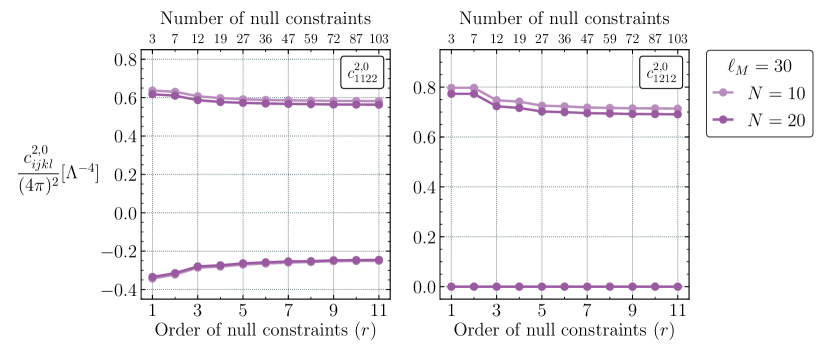
Figure 3: Upper/lower bounds on the amplitude coefficients for the bi-scalar theory, $c^{2,0}_{1212}$ and $c^{2,0}_{1122}$, in units of $(4\pi)^{2}$ and $\Lambda^{-4}$ resulting from our optimisation procedure as a function of the order of null constraints applied. The upper axis label indicates the number of independent null constraints appearing up to each order.

In this case, we go to the 11th order where there are 103 null constraints applied, and the result gradually levels off. We conclude that the bounds are

$$0 \leq\frac{c_{1212}^{2,0}}{(4\pi)^{2}}\leq\frac{0.691}{\Lambda^{4}}\,,$$ (70)

$$-\frac{0.246}{\Lambda^{4}} \leq\frac{c_{1122}^{2,0}}{(4\pi)^{2}}=\frac{c_{1221}^{2,0}}{(4\pi)^{2}}\leq\frac{0.563}{\Lambda^{4}}\,.$$ (71)

We also determine the 2-D allowed region in the space of $c_{1122}^{2,0}$ and $c_{1212}^{2,0}$, by maximizing many linear combinations in the form of $\alpha c_{1122}^{2,0}+\beta c_{1212}^{2,0}$. The result is shown in Figure 4, where successively darker shaded regions indicate the use of increasing orders of null constraints, where we have fixed $N=20$ and $\ell_{M}=30$.

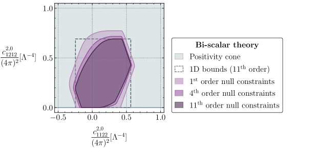
Figure 4: Allowed parameter space for the amplitude coefficients for the bi-scalar theory, $c^{2,0}_{1212}$ and $c^{2,0}_{1122}$, in units of $(4\pi)^{2}$ and $\Lambda^{-4}$ resulting from our optimisation procedure. Bounds obtained by employing null constraints at the 1${}^{\text{st}}$, 4${}^{\text{th}}$ and 11${}^{\text{th}}$ order are shown in successive darker purple shaded regions. For comparison, the grey shaded region shows the allowed half-space projected down from the positivity cone of the bi-scalar theory. The dotted lines delimit the region enclosed by the corresponding one dimensional bounds obtained with 11${}^{\text{th}}$ order null constraints shown in Figure 3.

The allowed region converges as we increase the null constraint order, and we do not expect significant improvements beyond the 11${}^{\text{th}}$ order. The new allowed region can be compared to the half-space that is allowed by traditional “lower” positivity bounds obtained from the positivity cone method Li:2021lpe , shaded in grey. The dashed lines also show the square region delimited by the 1D bounds in Eqs. (70) and  (71). We see that the 2D regions coincide along the line $c^{2,0}_{1212}=0$, where the traditional positivity bounds apply. The points where each coefficient is maximised also coincides with the 1D bounds that we obtained above, as expected. Overall, the true bounds in the 2D plane rule out a significant, additional portion of the parameter space with respect to the independent 1D case. Since they make use of the most information available, these are the strongest bounds on the bi-scalar EFT Wilson coefficients that have been found to date.

3 Upper bounds on Higgs scattering coefficients

Having established the formalism and gone through the warm-up examples, we now proceed to study the more realistic case of two Higgs boson scattering in the SMEFT. In this section, we identify relevant features of the theory and use them to develop the optimization procedure to bound the Wilson coefficients.

3.1 Effective operators for Higgs scattering

The Higgs field transforms as a complex doublet under the weak $\mathrm{SU}(2)$ gauge symmetry. To make contact with the real scalar scatterings that we have previously analysed, we parametrize the Higgs doublet with four real components

$$H=\frac{1}{\sqrt{2}}\begin{pmatrix}\phi_{1}+i\phi_{2}\\ \phi_{3}+i\phi_{4}\end{pmatrix}\,.$$ (72)

We consider the set of 2-to-2 scatterings $\phi_{i}\phi_{j}\to\phi_{k}\phi_{l}$, where $i,\,j,\,k,\,l$ runs from 1 to 4, and will compute the $s^{2}$ coefficients $c_{ijkl}^{2,0}$ defined in the last section from the effective Lagrangian. $SU(2)$ gauge invariance prevents the construction of an operator made out of three Higgs fields and derivatives, so there are no higher-derivative, three-point Higgs interactions in the massless limit that could contribute quadratically to the $s^{2}$ growth. This means that the only contributions to $c_{ijkl}^{2,0}$ come from single insertions of four-derivative dimension-8 operators Eboli:2006wa ; Almeida:2020ylr ; Li:2020gnx ; Murphy:2020rsh

$$\mathcal{O}^{(1)}_{H^{4}} =\left(D_{\mu}H^{\dagger}D_{\nu}H\right)\left(D^{\nu}H^{\dagger}D^{\mu}H\right)\,,$$ (73)

$$\mathcal{O}^{(2)}_{H^{4}} =\left(D_{\mu}H^{\dagger}D_{\nu}H\right)\left(D^{\mu}H^{\dagger}D^{\nu}H\right)\,,$$ (74)

$$\mathcal{O}^{(3)}_{H^{4}} =\left(D^{\mu}H^{\dagger}D_{\mu}H\right)\left(D^{\nu}H^{\dagger}D_{\nu}H\right)\,.$$ (75)

For convenience, we relabel the four real scalars in the Higgs doublet as

$$H=\frac{1}{\sqrt{2}}\begin{pmatrix}H^{1}_{1}+iH^{1}_{2}\\[2.84526pt] H^{2}_{1}+iH^{2}_{2}\end{pmatrix}\,,$$ (76)

and consider the contribution of the dimension-8 operators in Eqs. (73)–(75), to the four-Higgs scattering amplitude, $\mathcal{M}$. The $s^{2}$ coefficient of this amplitude can then be easily extracted:

$$a^{2,0\,abcd}_{\hskip 12.0ptIJKL} \equiv{1\over 2}\frac{{\rm d}^{2}}{{\rm d}s^{2}}\mathcal{M}\left(H_{I}^{a}H_{J}^{b}\to H_{K}^{c}H_{L}^{d}\right)$$

$$=\frac{1}{4}\delta_{IJ}\delta_{KL}\left[\delta_{ab}\delta_{cd}\left(C_{1}+C_{2}+2C_{3}\right)+\delta_{ad}\delta_{bc}\left(C_{1}-C_{2}\right)\right]$$

$$\quad+\frac{1}{4}\delta_{IK}\delta_{JL}\left[\delta_{ac}\delta_{bd}\left(2C_{1}+2C_{2}\right)+\left(\delta_{ad}\delta_{bc}+\delta_{ab}\delta_{cd}\right)\left(C_{2}-C_{1}\right)\right]$$

$$\quad+\frac{1}{4}\delta_{IL}\delta_{JK}\left[\delta_{ad}\delta_{bc}\left(C_{1}+C_{2}+2C_{3}\right)+\delta_{ab}\delta_{cd}\left(C_{1}-C_{2}\right)\right]\,,$$ (77)

where $C_{1}$, $C_{2}$ and $C_{3}$ are the Wilson coefficients for the operators $\mathcal{O}^{(1)}_{H^{4}}$, $\mathcal{O}^{(2)}_{H^{4}}$ and $\mathcal{O}^{(3)}_{H^{4}}$, respectively, $a,\,b,\,c,\,d=1,2$ are the weak $SU(2)$ indices and $I,\,J,\,K,\,L=1,2$ are the indices for the real and imaginary parts of a particular doublet component. We may convert the result in Eq. (77) into the $\left(\phi_{1},\,\phi_{2},\,\phi_{3},\,\phi_{4}\right)$ basis and obtain the corresponding coefficient, i.e., the $s^{2}$ coefficient of the subtracted full amplitude of $\phi_{i}\phi_{j}\to\phi_{k}\phi_{l}$ (Eq. (2-3)),

$$c^{2,0}_{ijkl}={1\over 2}\frac{{\rm d}^{2}}{{\rm d}s^{2}}B_{ijkl}(s,0)={1\over 2}\frac{{\rm d}^{2}}{{\rm d}s^{2}}\mathcal{M}\left(\phi_{i}\phi_{j}\to\phi_{k}\phi_{l}\right)=a^{2,0\,abcd}_{\hskip 12.0ptIJKL},$$ (78)

where $i=I+2(a-1),\,j=J+2(b-1),\,k=K+2(c-1),\,l=L+2(d-1)$ are the indices of the four real scalars in Eq. (72). This defines the linear map between the Wilson coefficients $C_{I}$ and the amplitude coefficients $c^{2,0}_{ijkl}$:

$$c^{2,0}_{1111} =C_{1}+C_{2}+C_{3}, c^{2,0}_{1122} =\frac{1}{2}\left(C_{1}+C_{3}\right),$$

$$c^{2,0}_{1212} =C_{2}, c^{2,0}_{1133} =\frac{1}{4}\left(C_{1}+C_{2}+2C_{3}\right),$$

$$c^{2,0}_{1313} =\frac{1}{2}\left(C_{1}+C_{2}\right), c^{2,0}_{1234} =\frac{1}{4}(C_{2}-C_{1}).$$ (79)

In Appendix C, we show how Lorentz symmetries, the Higgs internal symmetries and crossing symmetries can be used to either relate the rest of the $c^{2,0}_{ijkl}$ coefficients to the above six $c^{2,0}$ ones or set some of them to zero, which is consistent with and more instructive than simply listing all the $c^{2,0}_{ijkl}$ through Eq. (77-78). These six $c^{2,0}$ coefficients are of course not independent, as they can be expressed with just three Wilson coefficients, $C_{i}$.

The LP allows us to compute bounds for arbitrary linear combinations of $c^{2,0}_{ijkl}$. However, obtaining accurate numerical bounds can be relatively costly, so we will only explicitly present 1D and 2D bounds of the three $C_{I}$’s below.

3.2 Bounding the EFT coefficients of Higgs scattering

The one-sided positivity bounds for this sector of operators were been calculated in Refs. Zhang:2018shp ; Remmen:2019cyz using the scattering of electroweak states and read:

$$C_{2}\geq 0,\quad C_{1}+C_{2}\geq 0,\quad C_{1}+C_{2}+C_{3}\geq 0.$$ (80)

A subsequent analysis of the positivity cone in this sector was found to yield the same information Zhang:2020jyn , with the facets of the cone defined by the above inequalities. As such, these turn out to be be the optimal lower bounds that one can obtain from Higgs scattering.

In Section 2, we have set up a linear program method to obtain the two-sided positivity bounds on the Wilson coefficients from the sum rules along with the null constraints and the unitarity conditions in a general multi-field EFT. In Section 3.1, we have extracted the model-specific ingredients needed to perform the linear program for the SMEFT Higgs scatterings. We are now ready to apply our linear program to obtain bounds for the Higgs operators.

Instead of constraining the expansion coefficients of the amplitude such as $c^{2,0}_{1234}$, we want to directly bound the three dimension-8 Wilson coefficients $C_{1},C_{2},C_{3}$ in Eq. (73-75), using as much information as possible. The relations between the $c^{2,0}_{ijkl}$ and $C_{1},C_{2},C_{3}$ given in Eq. (79) and Appendix C can be reformulated as follows

$$\begin{gathered}C_{1}=-c^{2,0}_{1212}+2c^{2,0}_{1313},\quad C_{2}=c^{2,0}_{1212},\quad C_{3}=c^{2,0}_{1111}-2c^{2,0}_{1313}\,,\end{gathered}$$ (82)

$$\begin{gathered}c^{2,0}_{1122}=\frac{c^{2,0}_{1111}}{2}-\frac{c^{2,0}_{1212}}{2},\quad c^{2,0}_{1133}=c^{2,0}_{1144}=\frac{c^{2,0}_{1111}}{2}-\frac{c^{2,0}_{1313}}{2}\,,\\ c^{2,0}_{1414}=c^{2,0}_{1313},\quad c^{2,0}_{1234}=\frac{c^{2,0}_{1212}}{2}-\frac{c^{2,0}_{1313}}{2},\quad c^{2,0}_{1234}+c^{2,0}_{1243}=0\,,\\ c^{2,0}_{1324}=0,\quad c^{2,0}_{ijkl}=c^{2,0}_{ijkl}\Big{|}_{1\leftrightarrow 3,\ 2\leftrightarrow 4},\quad c^{2,0}_{ijkl}=c^{2,0}_{ijkl}\Big{|}_{1\leftrightarrow 2,\ 3\leftrightarrow 4}\,,\end{gathered}$$ (86)

where the last two equations denote that $c^{2,0}_{ijkl}$ is symmetric under the simultaneous interchange of $1\leftrightarrow 3$ and $2\leftrightarrow 4$, and the simultaneous interchange of $1\leftrightarrow 2$ and $3\leftrightarrow 4$. After expanding $c^{2,0}_{ijkl}$ into sums of $\rho^{ijkl}_{\ell,n}$ according to Eq. (4), the expressions for $C_{I}$ in Eq. (82), or linear combinations of them, are regarded as the objective functions to optimize, and the remaining relations in Eq. (86) become additional constraints in the LP problem.

Compared to the bi-scalar case, in addition to the null constraints on $\rho^{1111}_{\ell,n}$, $\rho^{1212}_{\ell,n}$,…, we now also include those containing 4 different scalar fields, i.e., the null constraints on $\rho^{1234}_{\ell,n}$, $\rho^{1324}_{\ell,n}$, $\rho^{1423}_{\ell,n}$,…, by the standard procedure of first choosing $i,j,k,l$ to be permutations of $1,2,3,4$ in Eq. (12) and then finding the linearly independent ones. Similar to the bi-scalar case, the first group of constraints on $\rho^{iiii}_{\ell,n}$ are connected to the constraints on $\rho^{iijj}_{\ell,n}$ and $\rho^{ijij}_{\ell,n}$ by the inequality $\big{|}\rho_{\ell}^{iijj}\big{|}\leq 1-\big{|}1-(\rho_{\ell}^{iiii}+\rho_{\ell}^{jjjj})/2\big{|}$. In turn, these are connected to the constraints for $\rho^{ijkl}_{\ell,n}$ by the inequality $\big{|}\rho_{\ell}^{ijkl}\big{|}\leq 1/4-\big{|}1/4-(\rho_{\ell}^{ijij}+\rho_{\ell}^{klkl})/2\big{|}$ (cf. Eq. (26)). Note that every link in this chain is indispensable for producing convergent and finite upper bounds of the objective functions, for the reason explained in Appendix B. The chain of unitarity conditions and null constraints are explicitly given by:

$$\left\{\begin{array}[]{lr}0\leq\rho^{iiii}_{\ell,n}\leq 2\,,\\ \sum\limits_{\ell=0,...,\ell_{M};\ell_{\infty}}(2\ell+1)\sum\limits_{n=1}^{N}\frac{1}{N}\left(\frac{n}{N}\right)^{r+2}C^{1111}_{r,i_{r}}(\ell)\rho^{iiii}_{\ell,n}=0\,,\end{array}\right.\hskip 11.99998pti\in\{1,2,3,4\}$$ (89)

$$\hskip 6.00006pt\big{|}\rho_{\ell}^{iijj}\big{|}\leq 1-\Big{|}1-\frac{\rho_{\ell}^{iiii}+\rho_{\ell}^{jjjj}}{2}\Big{|}\,,\hskip 20.00003pti,j\in\{1,2,3,4\}$$ (90)

$$\left\{\begin{array}[]{lr}0\leq\rho_{\ell,n}^{ijij}\leq\frac{1}{2}\,,\\[5.69054pt] \big{|}(\rho^{iijj}_{\ell,n}+\rho^{kkll}_{\ell,n})\pm(\rho^{iikk}_{\ell,n}+\rho^{jjll}_{\ell,n})\big{|}\leq 2\,,\\[2.84526pt] \sum\limits_{\ell=0,...,\ell_{M};\ell_{\infty}}\!\!(2\ell+1)\sum\limits_{n=1}^{N}\frac{1}{N}\left(\frac{n}{N}\right)^{r+2}\Big{[}C^{1122}_{r,i_{r}}(\ell)\rho_{\ell,n}^{iijj}+C^{1212}_{r,i_{r}}(\ell)\rho_{\ell,n}^{ijij}\Big{]}=0\,,\end{array}\right.\hskip 10.00002pti,j,k,l\in\{1,2,3,4\}$$ (94)

$$\hskip 6.00006pt\big{|}\rho_{\ell}^{1jkl}\big{|}\leq\frac{1}{4}-\Big{|}\frac{1}{4}-\frac{\rho_{\ell}^{1jij}+\rho_{\ell}^{klkl}}{2}\Big{|}\,,\hskip 20.00003ptj,k,l\in\{2,3,4\}$$ (95)

$$\left\{\begin{array}[]{lr}\sum\limits_{\ell=0,...,\ell_{M};\ell_{\infty}}(2\ell+1)\sum\limits_{n=1}^{N}\frac{1}{N}\left(\frac{n}{N}\right)^{r+2}\Big{[}C^{1234}_{r,i_{r}}(\ell)\rho_{\ell,n}^{1234}+C^{1324}_{r,i_{r}}(\ell)\rho_{\ell,n}^{1342}+C^{1423}_{r,i_{r}}(\ell)\rho_{\ell,n}^{1432}\Big{]}=0\,.\end{array}\right.$$ (97)

In the null constraints for 4 different fields (Eq. (95), we have set the first index of $\rho^{ijkl}_{\ell,n}$ to be $i=1$, since those are the only relevant variables that are related to our objective functions through Eq. (82) and Eq. (86). In the first two groups of null constraints, on the other hand, we need to include $i\neq 1$ since they are related to $\rho^{1jkl}_{\ell,n}$ through Eq. (95). $C^{1111}_{r,i_{r}}(\ell)$, $C^{1122}_{r,i_{r}}(\ell)$ and $C^{1212}_{r,i_{r}}(\ell)$ are the same as those appeared in Section 2.4 and 2.5. Similarly, $C^{1234}_{r,i_{r}}(\ell)$, $C^{1324}_{r,i_{r}}(\ell)$, $C^{1423}_{r,i_{r}}(\ell)$ are $\ell$ polynomials of degree less than or equal to $2r+2$, $r=1,2,...$ being the order of null constraints. In the case of 4 fields, the label for independent ones at each order is $i_{r}=1,2,...,2r+2$. For example, for $r=1$, $i_{r}=1$, we have

$$C^{1234}_{1,1} =-C^{1324}_{1,1}=-\ell^{4}-2\ell^{3}+\ell^{2}+2\ell\,,$$ (98)

$$C^{1423}_{1,1} =\big{(}1+(-1)^{\ell}\big{)}\Big{(}\ell^{4}+2\ell^{3}-13\ell^{2}-14\ell+24\Big{)}\,,$$ (99)

where the $(-1)^{\ell}$ originates from using the general symmetry of $\rho^{ijkl}_{\ell,n}=(-1)^{\ell}\rho^{ijlk}_{\ell,n}$ (Eq. (17)) to combine related coefficients.

We can further simplify the LP problem in an analogous way to what was done in Section 2.5, reducing the number of variables and constraints by using new variables $R^{ijkl}_{\ell,n}$ as certain linear combinations of $\rho^{ijkl}_{\ell,n}$. We show this process in Appendix D. This is very useful practically because, despite the efficiency of the modern linear program solvers, it becomes time and resource consuming to extract these bounds as the number of fields increases in the model. It is also worth noting that this change of variables we propose is completely general and does not rely on any symmetry of the scalar fields, such as the symmetry of Higgs. Now, the LP problem can be reformulated as

Variables

$$\hskip 11.99998ptR^{1111}_{\ell,n},\ R^{11ii}_{\ell,n},\ R^{1i1i}_{\ell,n},\ \rho^{1jkl}_{\ell,n}\,,\hskip 20.00003pti,j,k,l\in\{2,3,4\}$$ (100)

Maximize

$$\hskip 11.99998pt\sum_{I}\alpha_{I}C_{I}\,,~{}~{}~{}~{}\text{where}$$ (101)

$$\hskip 11.99998ptC_{1}=\frac{1}{\Lambda^{4}}\footnotesize{\text{$\sum\limits_{\ell=0,...,\ell_{M};\ell_{\infty}}$}}(2\ell+1)\footnotesize{\text{$\sum\limits_{n=1}^{N}\frac{1}{N}\frac{n}{N}$}}32(-R_{\ell,n}^{1212}+2R_{\ell,n}^{1313})\,,$$ (102)

$$\hskip 11.99998ptC_{2}=\frac{1}{\Lambda^{4}}\footnotesize{\text{$\sum\limits_{\ell=0,...,\ell_{M};\ell_{\infty}}$}}(2\ell+1)\footnotesize{\text{$\sum\limits_{n=1}^{N}\frac{1}{N}\frac{n}{N}$}}32R_{\ell,n}^{1212}\,,$$ (103)

$$\hskip 11.99998ptC_{3}=\frac{1}{\Lambda^{4}}\footnotesize{\text{$\sum\limits_{\ell=0,...,\ell_{M};\ell_{\infty}}$}}(2\ell+1)\footnotesize{\text{$\sum\limits_{n=1}^{N}\frac{1}{N}\frac{n}{N}$}}32(R_{\ell,n}^{1111}-2R_{\ell,n}^{1313})\,,$$ (104)

$$\hskip 11.99998pt\text{and}\,\alpha_{I}\text{ specify directions to optimze in }(C_{1},C_{2},C_{3})\text{ space}\,,$$

Subject to

$$\hskip 11.99998pt\mbox{Unitarity conditions and null constraints in Eq.(\ref{eq:higgsnc1}-\ref{eq:higgsnc2})}\,,$$

$$\hskip 11.99998pt\mbox{Additional constraints in Eq.(\ref{eq:addconstraint})}\,.$$

For example, to find the two-sided bounds on $C_{1}$, we choose $\alpha_{I}=(1,0,0)$ and $\alpha_{I}=(-1,0,0)$ respectively. In general, the $\alpha_{I}$ vector specifies which direction to optimize in the LP, and running $\alpha_{I}$ over different directions, we can plot the positivity bounds in 2D or 3D.

Fig 5 shows the individual results for the upper and lower bounds on $C_{1-3}$. The pairs of lines correspond to using $N=10$ and $20$, with fixed $\ell_{M}=30$, $\ell_{\infty}=100$. Rather coarse discretization values for the $\mu$ integral were used in order to have a reasonable computing time, and in Appendix E we discuss some convergence checks that were performed. The inaccuracy due to the discretisation results in looser bounds than the continuum limit $N\rightarrow\infty$, so the bounds we derive can be interpreted as conservative.

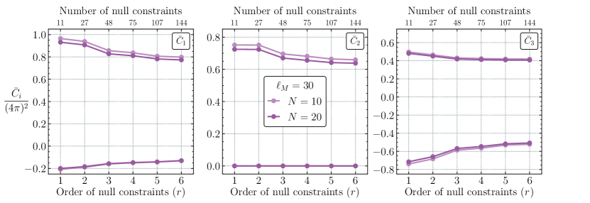
Figure 5: Upper/lower bounds on the dimension-8 Higgs scattering Wilson coefficients, $\bar{C}_{1}$, $\bar{C}_{2}$ and $\bar{C}_{3}$, in units of $(4\pi)^{2}$ resulting from our optimisation procedure as a function of the order of null constraints applied. The dimensionless coefficients are defined as $\bar{C}_{I}=C_{I}\Lambda^{4}$. The upper axis label indicates the total number of independent null constraints imposed at each order.

$$-\frac{0.130}{\Lambda^{4}} \leq\frac{C_{1}}{(4\pi)^{2}}\leq\frac{0.774}{\Lambda^{4}}\,,$$ (105)

$$0 \leq\frac{C_{2}}{(4\pi)^{2}}\leq\frac{0.638}{\Lambda^{4}}\,,$$ (106)

$$-\frac{0.508}{\Lambda^{4}} \leq\frac{C_{3}}{(4\pi)^{2}}\leq\frac{0.408}{\Lambda^{4}}\,.$$ (107)

In Figure 6, we show the 2D projections of the positivity bounds onto the planes spanned by two of $C_{1}$, $C_{2}$ and $C_{3}$. Each 2D plot is obtained by an angular optimization along 50 different directions. That is, one chooses 50 different combinations of $C_{i}$ and $C_{j}$, each of which picks out one direction, and for each combination or direction, one optimizes to get a upper bound. The numerical parameters chosen are $N=20$, $\ell_{M}=30$ and $\ell_{\infty}=100$. For the lower bounds, although we have not used the full positivity of the UV unitarity conditions, they are identical to those obtained via the convex cone approach, which does use the full UV positivity Zhang:2020jyn . However, now, using the non-positivity part of the UV unitarity conditions along with the null constraints, we have also derived the upper bounds for all of the Wilson coefficients $C_{i}$ for Higgs scattering, capping the Higgs positivity cone.

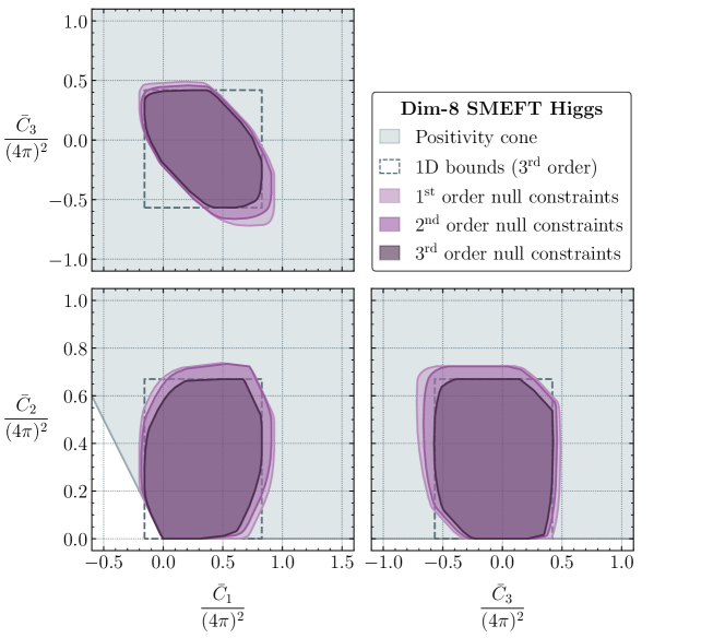
Figure 6: Allowed region in the two dimensional subspaces of $C_{1}$, $C_{2}$ and $C_{3}$, when applying 1${}^{\text{st}}$, 2${}^{\text{nd}}$ and 3${}^{\text{rd}}$ order null constraints (purple shaded) compared to the allowed regions by the positivity bounds on elastic scattering Zhang:2020jyn (grey shaded). The dimensionless coefficients are defined as $\bar{C}_{I}=C_{I}\Lambda^{4}$.

4 Comparison with experimental bounds and perturbative unitarity

Having successfully bounded the space of dimension-8 operators for Higgs scattering from first principles, we would like to compare the allowed space with the existing and future experimental limits on the operators in question. We will also compare the bounds arising from partial wave unitarity in the low energy EFT. To help us with the discussion, we will work in terms of the dimensionless Wilson coefficients, $\bar{C}_{I}$ since the bounds from experiment and partial wave unitarity depend on the cutoff $\Lambda_{\rm EFT}$. From here on, we identify $\Lambda_{\mathrm{{}_{EFT}}}$ and $\Lambda$, as per the discussion at the end of Section 2.3.

The Higgs scattering operators that we are interested in are subject to experimental constraints from LHC data, specifically from measurements of vector boson scattering (VBS). In this process a pair of weak bosons ($W$, $Z$ or photon) are emitted, one from each initial state quark, and undergo a hard, $2\to 2$ scattering that results in a distinctive signature of two weak bosons accompanied by two forward jets. This process is seen as a key probe of the gauge structure of the Standard Model that can test the unitarising properties of the Higgs boson exchange in weak boson scattering. It was measured for the first time in 2017 by the ATLAS and CMS collaborations CMS:2017fhs ; ATLAS:2019cbr , in the same-sign $WW$ channel and many other channels have since been observed and used to set bounds on anomalous quartic gauge couplings (aQGC). This process served as one of the primary motivations to experimentally probe dimension-8 operators in the SMEFT Yang:2020rjt ; Yang:2021pcf . This is because there are only a few operators at dimension-6 that can generate aQGC and they all lead to correlated effects in anomalous triple gauge couplings, electroweak precision observables or Higgs coupling modifications. Dimension-8 operators, on the other hand, can generate independent aQGCs. Therefore, although dimension-6 operators can impact VBS (See Gomez-Ambrosio:2018pnl ; Ethier:2021ydt for recent studies), it is expected that these operators will be better constrained elsewhere, hence opening up the opportunity to use this process as a probe of dimension-8 coefficients. The only exception to this argument applies to neutral triple gauge couplings, which are absent in both the SM and the SMEFT at dimension-6, hence also constitute a well motivated scenario in which to study dimension-8 operators Degrande:2013kka ; Senol:2018cks ; Rahaman:2018ujg ; Senol:2019swu ; Ellis:2019zex ; Ellis:2020ljj ; Fu:2021mub ; Lombardi:2021wug ; Jahedi:2022duc ; Senol:2022snc ; Ellis:2022zdw ; Spor:2022zob ; Degrande:2023iob .

In the unitary gauge, the three operators for which we obtain theoretical bounds specifically lead to four-derivative Higgs boson self-interactions, two-derivative interactions between pairs of Higgs and vector bosons, and a modification of the SM quartic gauge interactions. Although they do not explicitly contain extra derivatives, it is the latter that lead to unitarity-violating behaviour in 4-point, longitudinally polarised vector boson amplitudes, by spoiling the cancellations enforced by the SM gauge symmetries LlewellynSmith:1973yud ; Lee:1977eg ; Lee:1977yc . One can also understand this energy growth more intuitively by considering, e.g., the Feynman gauge, where the Goldstone modes are kept explicit. There, our operators also induce four-derivative contact interactions between the Goldstone boson components of the Higgs field. By the Goldstone boson equivalence theorem Cornwall:1974km , these can be identified with the longitudinal polarisations of the massive vector bosons of the SM. The strong energy growth with respect to the SM induced in fully longitudinal $2\to 2$ scattering amplitudes between $W$ and $Z$ bosons can be probed by measuring the high invariant mass region of the vector boson pair in VBS. This growth is the very same feature that we use to impose theoretical bounds on the coefficients, so it is interesting to compare the bounds that we have obtained with the current experimental sensitivity.

The LHC experiments use a basis of dimension-8 operators Eboli:2006wa ; Eboli:2016kko that predates even the determination of a complete non-redundant dimension-6 SMEFT basis. Our operators of interest, $\mathcal{O}^{(1)}_{H^{4}}$, $\mathcal{O}^{(2)}_{H^{4}}$ and $\mathcal{O}^{(3)}_{H^{4}}$ are identified with the operators $\mathcal{O}_{S,2}$, $\mathcal{O}_{S,0}$ and $\mathcal{O}_{S,1}$ of that basis, respectively. The LHC experiments have delivered a significant number of VBS analyses, deriving constraints on the coefficients of these operators. Among these, the most stringent bounds on the four-Higgs operators are reported by the CMS experiment, in a search for anomalous VBS production in semi-leptonic $WW$, $WZ$ and $ZZ$ final states CMS:2019qfk that we summarise in Table 1, for $\Lambda=1$ TeV.

The original set of dimension-8 operators was proposed only identified $\mathcal{O}_{S,0}$ and $\mathcal{O}_{S,1}$, with $\mathcal{O}_{S,2}$ only being added in follow up works some years later Eboli:2016kko . To our knowledge, the experimental collaborations have so far continued to only report results for $\mathcal{O}_{S,0}$ and $\mathcal{O}_{S,1}$. A recent phenomenological study Cappati:2022skp undertook a validation exercise reproducing the limits obtained by the CMS analysis, where a similar sensitivity to $\mathcal{O}_{S,1}$ was found for $\mathcal{O}_{S,2}$. We therefore assume that the experimental bound on $\mathcal{O}_{S,1}$ applies equally to $\mathcal{O}_{S,2}$ for our purposes, denoting the assumed bound by ‘$\ast$’.

Coefficient [0.5ex] ($\Lambda=1$ TeV)	Observed [0.5ex] kkk Bound CMS:2019qfk	HL-LHC projection Cappati:2022skp
		w/o unitarity	w unitarity
$\bar{C}_{1}$	k$[-3.4,\,3.4]^{\ast}$	$[-2.3,\,2.4]$	$[-4.8,\,5.2]$
$\bar{C}_{2}$	$[-2.7,\,2.7]$	$[-1.8,\,2.0]$	$[-2.6,\,3.3]$
$\bar{C}_{3}$	$[-3.4,\,3.4]$	$[-2.4,\,2.4]$	$[-5.8,\,6.1]$

Table 1: Summary of current and projected experimental bounds on four-Higgs dimension-8 operator coefficients. Current experimental limits are taken from Ref. CMS:2019qfk and future projections from a phenomenological analysis of Ref. Cappati:2022skp . The bounds on $\bar{C}_{1}$ denoted with an ‘$\ast$’ are not reported by the CMS analysis. Based on the results of Ref. Cappati:2022skp , we assume they are identical to those of $\bar{C}_{3}$.

The current experimental sensitivity lies around 2-4 TeV^-4 for the absolute value of the coefficients, and is dominated by the $WV$ channel, with one leptonically decaying $W$ boson and a hadronically decaying $W$ or $Z$ boson. The limits are symmetric around zero, which indicates that they are dominated by the quadratic, $\mathcal{O}(\Lambda^{-8})$ contribution of the coefficients to the VBS cross-section.

One of the challenges faced by the experimental collaborations when interpreting VBS data in terms of aQGC is that of unitarity violation. On one hand, sensitivity to aQGC is optimized by probing the high invariant-mass tails of VBS, which is already a rare process. On the other hand, the massive ($E^{4}$) energy growth of the underlying weak boson scattering amplitudes will eventually violate unitarity at some scale. Partial wave unitarity bounds on the dimension-8 aQGC Wilson coefficients were computed in Ref. Almeida:2020ylr , based on an analysis of $2\to 2$ Higgs and vector boson scattering amplitudes of various total charge and helicity. The bounds on our four-Higgs operators arise from the eigenvalues of the $J=0$ scattering matrices, and are summarised by

$$\begin{split}\big{|}\bar{C}_{1}+3\bar{C}_{2}+\bar{C}_{3}\big{|}&<96\pi\frac{\Lambda^{4}}{s^{2}},\\ \big{|}3\bar{C}_{1}+\bar{C}_{2}+\bar{C}_{3}\big{|}&<96\pi\frac{\Lambda^{4}}{s^{2}},\\ \big{|}5\bar{C}_{1}+3\bar{C}_{2}+7\bar{C}_{3}\big{|}&<96\pi\frac{\Lambda^{4}}{s^{2}}.\end{split}$$ (108)

These imply that, for bounds of around 3 TeV^-4 given in Table 1, unitarity is violated at a scale of 1.9-2.4 TeV. In VBS, the diboson invariant mass, $m_{VV}$ can be used as a proxy for the centre of mass energy, $\sqrt{s}$, of the $2\to 2$ sub-amplitude, and used to apply unitarity violation constraints on this process. Given that the analyses measure the $m_{VV}$ distribution out to around 2.5 TeV, the current sensitivity lies in a region that risks violating unitarity. Several procedures for mitigating this fact have been studied over the years, ranging from ad-hoc damping factors, physically motivated unitarization methods to simply forbidding the signal amplitudes from violating unitarity. None of these methods that modify the signal amplitudes are truly consistent with the model-independent SMEFT approach and the bounds reported in Table 1 are obtained without any unitarization method.

Another option is to consider limiting the energy reach of the data to a region where unitarity is not violated. Ref. Cappati:2022skp also studied the impact of unitarity bounds on the experimental constraints from VBS by computing them as a function of an upper cut on $m_{VV}$. Limiting the scattering energy simultaneously weakens the experimental and unitarity constraints on a given coefficients. New limits are then derived at the point where the experimentally derived bound with the upper cut on $m_{VV}$ is stronger than the unitarity bound obtained from identifying $\sqrt{s}=m_{VV}$ in Eq. (110). If there is no such point, then no limit can be derived. These bounds are summarised in the second and third columns of Table 1 and correspond to High-Luminosity LHC (HL-LHC) projected sensitivities. These show that unitarity considerations lead to order one effects on the experimental sensitivity on the Wilson coefficients.

We now turn to a comparison of our positivity bounds summarised in Eqs. (105)–(107) with the experimental sensitivity from current and projected VBS measurements as well as those arising from perturbative unitarity in Eq. (110). Our LP procedure produces bounds on individual coefficients, allowing the remaining coefficients to freely vary within their allowed range. The bounds are therefore the maximally conservative ones obtained from considering four-Higgs scattering amplitudes in the dimension-8 SMEFT. In contrast, the experimental constraints are obtained by setting all other coefficients to zero. Allowing all coefficients to vary would significantly reduce the sensitivity, and it may even be that a closed bound is not possible in this case. Furthermore, as discussed in Section 2.3, the experimental analyses bound the dimensionful combination, $\bar{C}_{I}/\Lambda^{4}$, such that the bound on the value of $\bar{C}_{I}$ varies depending on the assumed value of the EFT cutoff, $\Lambda$. This is reflected in Figure 7, which plots the experimental bounds as a function of $\Lambda$, as well as the $\Lambda$-independent bounds obtained from our numerical analysis. The solid grey line represents the current experimental limits that were obtained without mitigating possible unitarity violation in the signal modelling, while the dot-dashed grey lines show the projected HL-LHC bounds from Ref. Cappati:2022skp obtained with the unitarity mitigation prescription described above.

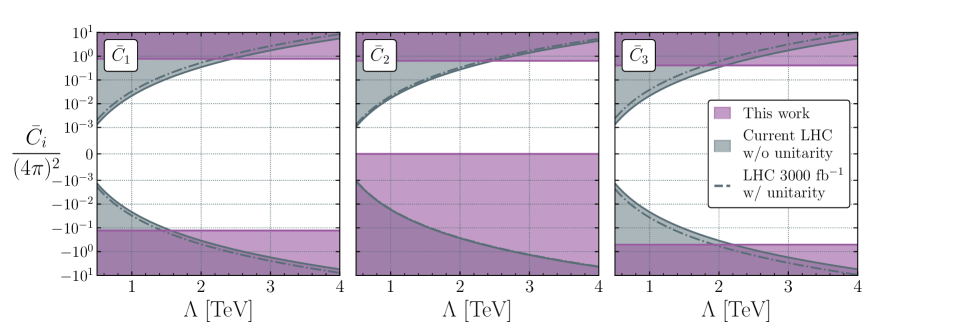
Figure 7: Upper and lower positivity bounds on the Higgs scattering Wilson coefficients obtained in this work (purple shaded) compared to the current CMS:2019qfk (grey shaded) and projected Cappati:2022skp (grey dashed) LHC exclusion limits from VBS measurements as a function of the EFT cutoff, $\Lambda$.

The fact that the HL-LHC projections are weaker than the current bounds underlines the significant effect that unitarity violation has on the prospects of probing these dimension-8 operators through VBS at the LHC.

One can see how the two-sided positivity bounds provide complementary information to the experimental limits. For instance, the lower bounds on $\bar{C}_{2}$ from the positivity cone immediately rules out half of the available parameter space. The new bounds obtained from our analysis cut out a further, significant portion of the parameter space and become stronger than the experimental limits for $\Lambda$ between 1.5 and 2.5 TeV, depending on the operator and the sign of its coefficient. Given that the experimental sensitivity – despite having assumed all other coefficients to be zero – implies unitarity violation around the same scale, our bounds appear highly competitive and even dominant over the experimental sensitivity. For example, if evidence for the presence of one of these operators were observed during the LHC lifetime, it would either imply an upper bound on the scale of new physics of order 1.5-2.5 TeV or a violation of unitarity, causality and/or locality in the UV. These processes are also therefore an interesting testbed for testing whether these fundamental principle hold true in physics beyond the SM.

In order to fairly compare our positivity bounds with those from perturbative unitarity, we infer ‘profiled’ unitarity bounds on each coefficient, in analogy with the fact that our bounds on a given coefficient allow the values of the others to float. Extremizing the value of each coefficient separately within the volume defined by Eq. (110) yields:

$$\big{|}\bar{C}_{1}\big{|},\big{|}\bar{C}_{3}\big{|}<0.6\times 96\pi\frac{\Lambda^{4}}{s^{2}},\quad\big{|}\bar{C}_{2}\big{|}<0.5\times 96\pi\frac{\Lambda^{4}}{s^{2}},$$ (109)

which we compare with our positivity bounds in Figure 8. The values of the Wilson coefficients are plotted in units of $(4\pi)^{2}$ and the unitarity bounds are shown as a function of $\sqrt{s}/\Lambda$, where $\sqrt{s}$ denotes the scale up to which one is willing to trust the EFT approximation for the tree-level scattering amplitudes that go into deriving them. The most aggressive unitarity bounds are then obtained by taking $\sqrt{s}=\Lambda$.

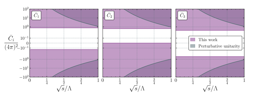
Figure 8: Upper and lower positivity bounds on the Higgs scattering Wilson coefficients obtained in this work (purple shaded) compared to the (tradiational) perturbative unitarity bounds obtained in the EFT (grey shaded) as a function of the ratio of centre of mass energy of the $2\to 2$ scattering, $\sqrt{s}$ relative to the EFT cutoff, $\Lambda$. The current LHC bounds do not impose unitarity on the EFT amplitudes while the projections take into account the unitarity bounds, providing the maximal limits that can be obtained while remaining consistent with perturbative unitarity.

From the conservative perspective of remaining agnostic about the possible values of the Wilson coefficients, our positivity bounds are stronger than the aggressive perturbative unitarity bounds by up to an order of magnitude. This is not to say that positivity is always more constraining than perturbative unitarity. Indeed, in certain directions of the parameter space, perturbative unitarity can yield a more powerful constraint. For example, by setting up our LP to maximise the specific linear combinations constrained in Eq. (110), we obtain the following positivity bounds, using the 6${}^{\text{th}}$ order null constraints and fixing $N=20$ and $\ell_{M}=30$:

$$\begin{split}0<\bar{C}_{1}+3\bar{C}_{2}+\bar{C}_{3}&<(4\pi)^{2}\times 2.42,\\ -(4\pi)^{2}\times 0.18<3\bar{C}_{1}+\bar{C}_{2}+\bar{C}_{3}&<(4\pi)^{2}\times 2.66,\\ -(4\pi)^{2}\times 1.07<5\bar{C}_{1}+3\bar{C}_{2}+7\bar{C}_{3}&<(4\pi)^{2}\times 5.89.\end{split}$$ (110)

Comparing the numbers to the most optimistic unitarity bound of $96\pi=1.91\times(4\pi)^{2}$, we see that for these particular directions, our upper bound from positivity is slightly weaker for the first two and about a factor of 3 weaker for the third. However, the lower bounds are considerably stronger. The first direction is bounded to be positive by the Higgs positivity cone, since it is a positive linear combination of $\bar{C}_{2}$ and $\bar{C}_{1}+\bar{C}_{2}+\bar{C}_{3}$, both of which are positive (See Eq. (80)). The others are not bounded by the positivity cone and hence can only be constrained by our two-sided approach.

Overall, it is clear that our positivity bounds provide highly complementary information on the viable space for dimension-8 operators that mediate Higgs scattering amplitudes to experimental and unitarity-based probes. Since they have a completely independent origin, they can be used as part of a data interpretation, i.e., by including them as part of the statistical prior to obtain tighter bounds on the Wilson coefficient space, adding only the relatively weak assumptions of unitarity, causailty and locality in the UV. Since the constraints can be stronger than perturbative unitarity, they may help experimental collaborations to avoid the recurrent issues of unitarity violation in the EFT interpretations of VBS measurements.

Appendix A Partial wave unitarity

Partial wave unitarity comes from the fact that in a scattering angular momentum is conserved, so the S-matrix can be block-diagonalized into different angular momenta: $S_{\ell}S^{\dagger}_{\ell}=I_{\ell}$. In this appendix, we first review an explicit derivation of the full partial wave unitarity conditions starting from the full scattering amplitudes, based largely on Ref Soldate:1986mk . Then, we derive a set of linear, two-sided unitarity conditions from full partial wave unitarity that can be easily implemented in our linear programming to constrain the Wilson coefficients using the dispersion relations.

A.1 Review

We work in 4 dimensions and evaluate amplitudes in the center of mass frame. The amplitude for a scalar $2\to 2$ scattering process, $ij\to kl$, can be decomposed into partial waves,

$$A_{ijkl}(\theta)\equiv\bra{{\bf\it i}}T\ket{{\bf\it f}}=16\pi\sum_{\ell=0}^{\infty}a_{\ell}^{ijkl}\quantity(2\ell+1)P_{\ell}(\cos{\theta})\,,$$ (111)

where ${\bf\it i}$ and ${\bf\it f}$ denote the two particle states $ij$ and $kl$, respectively, both of which consist of a pair of states in a back-to-back momentum configuration. $\theta$ is the polar angle between the $\hat{i}$ and $\hat{f}$ directions and we use the standard convention for Legendre polynomials where $P_{\ell}(1)=1$. From the unitarity of the $S$-matrix, we have

$$\bra{{\bf\it i}}T\ket{{\bf\it f}}-\bra{{\bf\it f}}T\ket{{\bf\it i}}^{*}=i\sum_{{\bf\it x}}\bra{{\bf\it i}}T\ket{{\bf\it x}}\bra{{\bf\it f}}T\ket{{\bf\it x}}^{*}(2\pi)^{4}\delta^{4}(p_{{\bf\it x}}-p_{{\bf\it i}})\,,$$ (112)

where the ${\bf\it x}$ summation includes both the sum over all possible intermediate states and the integration over their phase space. If the theory is time-reversal (CP) invariant, $A^{klij}=A^{ijkl}$, then the LHS of Eq. (112) becomes

$$\mathrm{LHS}=2i\,\mathrm{Im}A_{ijkl}=32i\,\pi\sum_{\ell=0}^{\infty}\mathrm{Im}a_{\ell}^{ijkl}\quantity(2\ell+1)P_{\ell}(\cos{\theta})\,.$$ (113)

For every phase space configuration of an intermediate state, ${\bf\it x}$, there exists a set of configurations that are related to it by an overall spatial rotation, $R(\Omega_{n})$, which can be characterised by its action on $\hat{i}$, rotating it to a new direction, $\hat{n}$. Denoting $\{X\}$ as the set of intermediate states that are not related by an overall rotation, each state ${\bf\it x}$ can be specified by $\{X,\Omega_{n}\}$. Now the RHS of Eq. (112) can be written as

$$\mathrm{RHS}=i\sum_{X}\int\differential\Omega_{n}\bra{{\bf\it i}}T\ket{X,\Omega_{n}}\bra{{\bf\it f}}T\ket{X,\Omega_{n}}^{*}(2\pi)^{4}\delta^{4}(p_{X}-p_{{\bf\it i}}),$$ (114)

where the integration over the solid angle of $\hat{n}$ has been factored out of the overall phase space integral. We can then expand each intermediate amplitude into partial waves

$$\bra{{\bf\it i}}T\ket{X,\Omega_{n}}=16\pi\sum_{\ell=0}^{\infty}a_{\ell}^{ij\rightarrow X}\quantity(2\ell+1)P_{\ell}(\cos{\theta_{in}})\,,$$ (115)

where $\cos\theta_{in}=\hat{i}\cdot\hat{n}$, and do the same for $\bra{{\bf\it f}}T\ket{X,\Omega_{n}}$. Using geometric relations and the addition formula for Legendre polynomials

$$\cos\theta_{fn} =\cos\theta\cos\theta_{in}+\sin\theta\sin\theta_{in}\cos\phi_{fn},$$ (116)

$$P_{\ell}(\cos\theta_{fn}) =P_{\ell}(\cos\theta)P_{\ell}(\cos\theta_{in})+2\!\sum_{m=1}^{\ell}\!\frac{(l-m)!}{(l+m)!}P_{\ell}^{m}(\cos\theta)P_{\ell}^{m}(\cos\theta_{in})\cos(m\phi_{fn}),$$ (117)

and evaluating the $\Omega_{n}$ integral in Eq. (114), we get

$$\mathrm{RHS}=i(16\pi)^{2}(4\pi)\sum_{\ell=0}^{\infty}\sum_{X}a_{\ell}^{ij\rightarrow X}\quantity(a_{\ell}^{kl\rightarrow X})^{*}\quantity(2\ell+1)P_{\ell}(\cos{\theta})(2\pi)^{4}\delta^{4}(p_{X}-p_{{\bf\it i}})\,.$$ (118)

Comparing Eq. (113) and Eq. (118), we obtain the partial wave unitarity condition

$$\mathrm{Im}a_{\ell}^{ijkl}=32\pi^{2}\sum_{X}a_{\ell}^{ij\rightarrow X}\quantity(a_{\ell}^{kl\rightarrow X})^{*}(2\pi)^{4}\delta^{4}(p_{X}-p_{{\bf\it i}})\,.$$ (119)

For the special case of $X=\{mn\}$, i.e., when the intermediate state is also a two scalar field state, $\sum_{X}$ reduces to a phase space integral over the magnitude of the momentum

$$32\pi^{2}\,\eta_{mn}\int\frac{p_{f}^{2}\differential p_{f}}{(2\pi)^{6}}\frac{1}{(2E_{p_{f}})^{2}}a_{\ell}^{ijmn}\quantity(a_{\ell}^{klmn})^{*}(2\pi)^{4}\delta(2E_{p_{f}}-E_{i})$$ (120)

$$=\, \eta_{mn}\,a_{\ell}^{ijmn}\quantity(a_{\ell}^{klmn})^{*}\,,\hskip 20.00003pt\mbox{(massless limit)}$$ (121)

where $\eta_{mn}$ is a prefactor that accounts for identical final-state particles: $\eta_{mn}=1$ for $m\neq n$ and $\eta_{mn}=1/2$ for $m=n$. (For massive particles, we can again get Eq. (120) if the partial wave expansion is defined with an extra kinematic factor.) For the rest of the positive weighted sum in Eq. (119), we can define the normalized $a_{\ell}^{ij,kl\rightarrow X}$ to have unit weight for our purposes. We can now write the unitarity condition in a more compact form

$$\mathrm{Im}a_{\ell}^{ijkl}=\sum_{mn}\,\eta_{mn}a_{\ell}^{ijmn}\quantity(a_{\ell}^{klmn})^{*}+\sum_{X\neq mn}a_{\ell}^{ij\rightarrow X}\quantity(a_{\ell}^{kl\rightarrow X})^{*}\,.$$ (122)

In the text, sometimes we omit the prefactor $\eta_{mn}$ and refer to this condition simply as $\mathrm{Im}a_{\ell}^{ijkl}=\sum^{\prime}_{X}a_{\ell}^{ij\rightarrow X}\quantity(a_{\ell}^{kl\rightarrow X})^{*}$.

A.2 Linear unitarity conditions

From partial wave unitarity (122), we can derive some linear unitarity conditions on the imaginary part of partial wave amplitude $\mathrm{Im}a_{\ell}^{ijkl}$, which can be easily fed into the linear programs to constrain the EFT coefficients. While the linear conditions presented below are already very constraining, it is likely that we have not exhausted all possible linear unitarity conditions.
• Individual partial amplitudes
First, we derive simple two-sided constraints on individual $\mathrm{Im}a^{ijkl}$, making use of the positive nature of the sum on the right hand side of (122) for elastic scatterings.

For the process of $ii\to ii$, picking out only $X=ii$ for the intermediate states gives

$$\mathrm{Im}a_{\ell}^{iiii}\geq\frac{1}{2}|a_{\ell}^{iiii}|^{2}=\frac{1}{2}\left(\mathrm{Im}a_{\ell}^{iiii}\right)^{2}+\frac{1}{2}\left(\mathrm{Re}a_{\ell}^{iiii}\right)^{2}$$

$$\hskip 40.00006pt\Rightarrow~{}~{}~{}0\leq\mathrm{Im}a_{\ell}^{iiii}\leq 2,$$ (123)

picking out $X=ii,jj$ gives

$$\mathrm{Im}a_{\ell}^{iiii}\geq\frac{|a_{\ell}^{iiii}|^{2}}{2}+\frac{|a_{\ell}^{iijj}|^{2}}{2}=\frac{\left(\mathrm{Im}a_{\ell}^{iiii}\right)^{2}}{2}+\frac{\left(\mathrm{Re}a_{\ell}^{iiii}\right)^{2}}{2}+\frac{\big{(}\mathrm{Im}a_{\ell}^{iijj}\big{)}^{2}}{2}+\frac{\big{(}\mathrm{Re}a_{\ell}^{iijj}\big{)}^{2}}{2}\,,$$

$$\hskip 112.00014pt\Rightarrow~{}~{}~{}-1\leq\mathrm{Im}a_{\ell}^{iijj}\leq 1\,,$$ (124)

For the process of $ij\to ij$, picking out $X=ij,ji$ leads to

$$\mathrm{Im}a_{\ell}^{ijij}\geq|a_{\ell}^{ijij}|^{2}+|a_{\ell}^{ijji}|^{2}=\big{(}\mathrm{Im}a_{\ell}^{ijij}\big{)}^{2}+\big{(}\mathrm{Re}a_{\ell}^{ijij}\big{)}^{2}+\big{(}\mathrm{Im}a_{\ell}^{ijji}\big{)}^{2}+\big{(}\mathrm{Re}a_{\ell}^{ijji}\big{)}^{2}\geq 2\big{(}\mathrm{Im}a_{\ell}^{ijij}\big{)}^{2}$$

$$\hskip 136.00026pt\Rightarrow~{}~{}~{}0\leq\mathrm{Im}a_{\ell}^{ijij}\leq\frac{1}{2}\,,$$ (125)

where we have used the fact that $a^{ijji}_{\ell}=(-1)^{\ell}\,a^{ijij}_{\ell}$. Picking out multiple distinct intermediate states $X=ij,ji,kl,lk$ ($kl,lk\neq ij$) gives

$$\mathrm{Im}a_{\ell}^{ijij} \geq\big{|}a_{\ell}^{ijij}\big{|}^{2}+\big{|}a_{\ell}^{ijji}\big{|}^{2}+\big{|}a_{\ell}^{ijkl}\big{|}^{2}+\big{|}a_{\ell}^{ijlk}\big{|}^{2}=2\big{|}a_{\ell}^{ijij}\big{|}^{2}+2\big{|}a_{\ell}^{ijkl}\big{|}^{2}$$

$$\geq 2\big{(}\mathrm{Im}a_{\ell}^{ijij}\big{)}^{2}+2\big{(}\mathrm{Im}a_{\ell}^{ijkl}\big{)}^{2}~{}~{}~{}~{}\Rightarrow~{}~{}~{}-\frac{1}{4}\leq\mathrm{Im}a_{\ell}^{ijkl}\leq\frac{1}{4}\,,$$ (126)

where we have again used $a^{ijkl}_{\ell}=(-1)^{\ell}\,a^{ijlk}_{\ell}$. In the numerical LP, we will use conditions (123) and (125), but will not use conditions (124) and (126), as we can obtain stronger conditions than (124) and (126), as shown below.

• Mixing different partial amplitudes
Given the above simple bounds, now we show that some of them can be further enhanced with a more careful treatment of unitaritiy conditions (122).

First, note that a simple re-arrangement of Eq. (122) for $iiii$ gives

$$\quantity(2-\mathrm{Im}a_{\ell}^{iiii})=\frac{1}{2}\quantity(2-\mathrm{Im}a_{\ell}^{iiii})^{2}+\frac{1}{2}\quantity(\mathrm{Re}a_{\ell}^{iiii})^{2}+\sum_{X\neq ii}\!\!{}^{\prime}\big{|}a_{\ell}^{ii\rightarrow X}\big{|}^{2}\,.$$ (127)

On the other hand, Eq. (122) for $iijj$ can be explicitly written as

$$\mathrm{Im}a_{\ell}^{iijj} =\frac{1}{2}a_{\ell}^{iiii}\big{(}a_{\ell}^{jjii}\big{)}^{*}+\frac{1}{2}a_{\ell}^{iijj}\big{(}a_{\ell}^{jjjj}\big{)}^{*}+\sum_{X\neq ii,jj}\!\!\!\!{}^{\prime}~{}a_{\ell}^{ii\rightarrow X}\big{(}a_{\ell}^{jj\rightarrow X}\big{)}^{*}$$ (128)

$$=\frac{1}{2}\mathrm{Im}a_{\ell}^{iijj}\big{(}\mathrm{Im}a_{\ell}^{iiii}+\mathrm{Im}a_{\ell}^{jjjj}\big{)}+\frac{1}{2}\big{(}\mathrm{Re}a_{\ell}^{iiii}\mathrm{Re}a_{\ell}^{jjii}+\mathrm{Re}a_{\ell}^{iijj}\mathrm{Re}a_{\ell}^{jjjj}\big{)}$$

$$\hskip 20.00003pt+\sum_{X\neq ii,jj}\!\!\!\!{}^{\prime}~{}\Big{(}\mathrm{Im}\,a_{\ell}^{ii\rightarrow X}\mathrm{Im}\,a_{\ell}^{jj\rightarrow X}+\mathrm{Re}\,a_{\ell}^{ii\rightarrow X}\mathrm{Re}\,a_{\ell}^{jj\rightarrow X}\Big{)}\,,$$ (129)

where we have used the time-reversal invariance $a_{\ell}^{iijj}=a_{\ell}^{jjii}$ for the first term on the second line, and the imaginary terms on the right hand side of Eq. (128) must cancel because $\mathrm{Im}a_{\ell}^{iijj}$ is real. A simple rearrangement of Eq. (129) then gives

$$-\mathrm{Im}a_{\ell}^{iijj} =-\frac{1}{2}\mathrm{Im}a_{\ell}^{iijj}\quantity(\quantity(2-\mathrm{Im}a_{\ell}^{iiii})+\big{(}2-\mathrm{Im}a_{\ell}^{jjjj}\big{)})+\frac{1}{2}\big{(}\mathrm{Re}a_{\ell}^{iiii}\mathrm{Re}a_{\ell}^{jjii}+\mathrm{Re}a_{\ell}^{iijj}\mathrm{Re}a_{\ell}^{jjjj}\big{)}$$

$$\hskip 20.00003pt+\sum_{X\neq ii,jj}\!\!\!\!{}^{\prime}~{}\Big{(}\mathrm{Im}\,a_{\ell}^{ii\rightarrow X}\mathrm{Im}\,a_{\ell}^{jj\rightarrow X}+\mathrm{Re}\,a_{\ell}^{ii\rightarrow X}\mathrm{Re}\,a_{\ell}^{jj\rightarrow X}\Big{)}\,.$$ (130)

Notice that conditions (129) and (130) are structurely very similar if we swap $\mathrm{Im}a^{iiii}_{\ell}\leftrightarrow(2-\mathrm{Im}a^{iiii}_{\ell})$. This allows us to obtain an inequality using a technique similar to that leads to Eq. (21) and the Cauchy-Schwarz inequality. More explicitly,

$$\big{|}\mathrm{Im}a_{\ell}^{iijj}\big{|}^{2} \leq\Bigg{(}\frac{(2-\mathrm{Im}a^{iiii}_{\ell})^{2}}{2}+\frac{(\mathrm{Im}a^{iijj}_{\ell})^{2}}{2}+\frac{(\mathrm{Re}a_{\ell}^{iiii})^{2}}{2}+\frac{(\mathrm{Re}a_{\ell}^{iijj})^{2}}{2}+\sum_{X\neq ii,jj}\!\!\!\!{}^{\prime}\;\big{|}a_{\ell}^{ii\rightarrow X}\big{|}^{2}\Bigg{)}$$

$$\times\Bigg{(}\frac{(\mathrm{Im}a^{jjii}_{\ell})^{2}}{2}+\frac{(2-\mathrm{Im}a^{jjjj}_{\ell})^{2}}{2}+\frac{(\mathrm{Re}a_{\ell}^{jjii})^{2}}{2}+\frac{(\mathrm{Re}a_{\ell}^{jjjj})^{2}}{2}+\sum_{X\neq ii,jj}\!\!\!\!{}^{\prime}\;\big{|}a_{\ell}^{jj\rightarrow X}\big{|}^{2}\Bigg{)}$$

$$=\big{(}2-\mathrm{Im}a^{iiii}_{\ell}\big{)}\big{(}2-\mathrm{Im}a^{jjjj}_{\ell}\big{)}\leq\Big{(}2-\frac{\mathrm{Im}a^{iiii}_{\ell}+\mathrm{Im}a^{jjjj}_{\ell}}{2}\Big{)}^{2}\,,$$ (131)

where in the last line we have used Eq. (127). Taking the square root, we get a linear inequality

$$\big{|}\mathrm{Im}a_{\ell}^{iijj}\big{|}\leq 2-\frac{\mathrm{Im}a^{iiii}_{\ell}+\mathrm{Im}a^{jjjj}_{\ell}}{2}\,.$$ (132)

For unitarity conditions with $a_{\ell}^{ijij}$ and $a_{\ell}^{i\neq j\neq k\neq l}$, we can analogously obtain

$$\big{|}\mathrm{Im}a_{\ell}^{ijkl}\big{|}\leq\frac{1}{2}-\frac{\mathrm{Im}a_{\ell}^{ijij}+\mathrm{Im}a_{\ell}^{klkl}}{2}\,.$$ (133)

Recall that, in the main text, we have established a similar set of inequalities (22) for $\mathrm{Im}a^{iijj}_{\ell}$ and $\mathrm{Im}a^{ijkl}_{\ell}$:

$$\big{|}\mathrm{Im}a^{iijj}_{\ell}\big{|}\leq\frac{\mathrm{Im}a^{iiii}_{\ell}+\mathrm{Im}a^{jjjj}_{\ell}}{2},~{}~{}~{}~{}~{}~{}\big{|}\mathrm{Im}a^{ijkl}_{\ell}\big{|}\leq\frac{\mathrm{Im}a^{ijij}_{\ell}+\mathrm{Im}a^{klkl}_{\ell}}{2}\,.$$ (134)

Combining Eqs. (132-134), we conclude

$$\big{|}\mathrm{Im}a_{\ell}^{iijj}\big{|} \leq 1-\Big{|}1-\frac{\mathrm{Im}a_{\ell}^{iiii}+\mathrm{Im}a_{\ell}^{jjjj}}{2}\Big{|}\,,$$ (135)

$$\big{|}\mathrm{Im}a_{\ell}^{ijkl}\big{|} \leq\frac{1}{4}-\Big{|}\frac{1}{4}-\frac{\mathrm{Im}a_{\ell}^{ijij}+\mathrm{Im}a_{\ell}^{klkl}}{2}\Big{|},$$ (136)

which are stronger than Eqs. (124) and (126).

• Special inequalities with four fields
For the case of 4 fields , we can derive some extra linear constraints. To highlight the variables whose constraints we are after, let us denote $\mathrm{Im}a^{1122}_{\ell}$, $\mathrm{Im}a^{1133}_{\ell}$, $\mathrm{Im}a^{2244}_{\ell}$ and $\mathrm{Im}a^{3344}_{\ell}$ as ${\cal A}$, ${\cal B}$, ${\cal C}$ and ${\cal D}$ respectively. After some simple re-arrangements, the unitarity condition (Eq. (122)) for the case of $ijkl=1111,4444,1144$ can be written as, respectively,

$$\big{(}1-\mathrm{Im}a^{1111}_{\ell}\big{)}^{2}+\big{(}\mathrm{Im}a^{1144}_{\ell}\big{)}^{2} =1-{\cal A}^{2}-{\cal B}^{2}-2{\cal S}^{1111}\,,$$ (137)

$$\big{(}1-\mathrm{Im}a^{4444}_{\ell}\big{)}^{2}+\big{(}\mathrm{Im}a^{1144}_{\ell}\big{)}^{2} =1-{\cal C}^{2}-{\cal D}^{2}-2{\cal S}^{4444}\,,$$ (138)

$$\mathrm{Im}a^{1144}_{\ell}\big{(}(1-\mathrm{Im}a^{1111}_{\ell})+(1-\mathrm{Im}a^{4444}_{\ell})\big{)} ={\cal A}{\cal C}+{\cal B}{\cal D}+2{\cal S}^{1144}\,,$$ (139)

where we have introduced the shorthand

$${\cal S}^{iijj}=\sum_{X}{}{}^{\prime}\;\mathrm{Re}\,a_{\ell}^{ii\rightarrow X}\mathrm{Re}\,a_{\ell}^{jj\rightarrow X}+\sum_{X\neq 11,22,33,44}{}^{\prime}~{}~{}~{}~{}\mathrm{Im}\,a_{\ell}^{ii\rightarrow X}\mathrm{Im}\,a_{\ell}^{jj\rightarrow X}\,.$$ (140)

Combining the three equations as (137)$+$(138)$-2$(139) and using the fact that ${\cal S}^{1144}\geq-\sqrt{{\cal S}^{1111}{\cal S}^{4444}}$, we can obtain

$$\,2-({\cal A}+{\cal C})^{2}-({\cal B}+{\cal D})^{2}$$

$$= \,\big{(}1-\mathrm{Im}a^{1111}_{\ell}-\mathrm{Im}a^{1144}_{\ell}\big{)}^{2}+\big{(}1-\mathrm{Im}a^{4444}_{\ell}-\mathrm{Im}a^{1144}_{\ell}\big{)}^{2}+2\big{(}{\cal S}^{1111}+{\cal S}^{4444}+2{\cal S}^{1144}\big{)}$$

$$\geq \,2\big{(}\sqrt{{\cal S}^{1111}}-\sqrt{{\cal S}^{4444}}\big{)}^{2}\geq 0\,,$$ (141)

Similarly, combining the three equations as (137)$+$(138)$+2$(139) and using the fact that ${\cal S}^{1144}\leq\sqrt{{\cal S}^{1111}{\cal S}^{4444}}$, we have

$$({\cal A}-{\cal C})^{2}+({\cal B}-{\cal D})^{2}\leq 2\,,$$ (142)

In the numerical LP, we will use the linear conditions that can be inferred from conditions (141) and (142) respectively:

$$|\mathrm{Im}a^{1122}_{\ell}+\mathrm{Im}a^{1133}_{\ell}+\mathrm{Im}a^{2244}_{\ell}+\mathrm{Im}a^{3344}_{\ell}| \leq 2\,,$$ (143)

$$|\mathrm{Im}a^{1122}_{\ell}-\mathrm{Im}a^{1133}_{\ell}-\mathrm{Im}a^{2244}_{\ell}+\mathrm{Im}a^{3344}_{\ell}| \leq 2\,.$$ (144)

The above two conditions are the strongest in the 2D subspace furnished by $({\cal A}+{\cal D})$ and $({\cal B}+{\cal C})$ from the unitarity conditions in the form of (137) to (139). Obviously, for general $i\neq j\neq k\neq l$, the same result can be formulated as

$$\big{|}(\mathrm{Im}a^{iijj}_{\ell}+\mathrm{Im}a^{kkll}_{\ell})\pm(\mathrm{Im}a^{iikk}_{\ell}+\mathrm{Im}a^{jjll}_{\ell})\big{|}\leq 2\,.$$ (145)

Appendix B Existence of upper bounds: simple analytical example

In this appendix, we shall use a simple example to illustrate why the LP problem (29-35) leads to upper bounds on the amplitude coefficients. We will not attempt to use all available null constraints and unitarity conditions, but utilize just a few conditions to establish the existence of an upper bound, the upshot being that we can show this analytically. Furthermore, in the numerical LP, we have to truncate the partial waves at a finite order $\ell_{M}$, while in the analytical example below, we can sum over all partial waves, and find that the result does not diverge as $\ell$ goes to infinity. This, together with our numerical convergence study in Appendix E justifies the finite $\ell$ truncation in our numerical results.

We shall take the $c_{1212}^{2,0}$ coefficient as an example, analytically bounding it from the above. The sum rule for this coefficient is given by

$$c_{1212}^{2,0}=\frac{1}{\Lambda^{4}}\,32\sum_{\ell\geq 0}(2\ell+1)\int_{0}^{1}\differential z\,z\,\rho_{\ell}^{1212}(z)\,,$$ (146)

where we have changed the integration variable from $\mu$ to $z={\Lambda^{2}}/{\mu}$ in Eq. (28). Likewise, the first order null constraint for $\rho^{1111}_{\ell}$ can be written as

$$\sum_{\ell\geq 0}(2\ell+1)\int_{0}^{1}\differential z\,z^{3}(\ell^{4}+2\ell^{3}-7\ell^{2}-8\ell)\rho^{1111}_{\ell}(z)=0\,.$$ (147)

By $\rho_{\ell}^{ijkl}=(-1)^{\ell}\rho_{\ell}^{jikl}$, we can infer that $\rho^{1111}_{\ell={\rm odd}}=0$. Moving the negative $\ell=2$ term to the right hand side ($0\leq\rho^{1111}_{\ell}\leq 2$) and using the unitarity condition of $\rho^{1111}_{2}\leq 2$, we get

$$\sum_{\ell\geq 4}(2\ell+1)\int_{0}^{1}\differential z\,z^{3}(\ell^{4}+2\ell^{3}-7\ell^{2}-8\ell)\rho^{1111}_{\ell}(z)=\int_{0}^{1}\differential z\,z^{3}60\rho^{1111}_{2}(z)\leq{30}\,.$$ (148)

That is, an infinite positive sum converges to a finite number, which implies that $\int_{0}^{1}\!\differential z\,z^{3}\rho^{1111}_{\ell}$ must be sufficiently small at large $\ell$, sometimes known as low spin dominance. We stress that this is a result of null constraints. Since $\rho^{1111}_{\ell}$ and $\rho^{2222}_{\ell}$ satisfy exactly the same constraints, we can replace $\rho^{1111}_{\ell}$ with $(\rho^{1111}_{\ell}+\rho^{2222}_{\ell})/2$ in the inequality above, and further use it to constrain a similar positive sum on $\rho^{1122}_{\ell}$ through $|\rho^{1122}_{\ell}|\leq(\rho^{1111}_{\ell}+\rho^{2222}_{\ell})/2$,

$$\sum_{\ell\geq 4}(2\ell+1)\int_{0}^{1}\differential z\,z^{3}(\ell^{4}+2\ell^{3}+\ell^{2})\,\quantity|\rho^{1122}_{\ell}(z)|$$ (149)

$$\leq \,\frac{5}{3}\sum_{\ell\geq 4}(2\ell+1)\int_{0}^{1}\differential z\,z^{3}(\ell^{4}+2\ell^{3}-7\ell^{2}-8\ell)\,\quantity|\rho^{1122}_{\ell}(z)|$$ (150)

$$\leq \,\frac{5}{3}\sum_{\ell\geq 4}(2\ell+1)\int_{0}^{1}\differential z\,z^{3}(\ell^{4}+2\ell^{3}-7\ell^{2}-8\ell)\,\frac{\rho^{1111}_{\ell}(z)+\rho^{2222}_{\ell}(z)}{2}\leq\,\frac{5}{3}\times{30}={50}\,.$$ (151)

The sum (149) appears in one of the first order null constraints for $\rho^{1122}_{\ell}$ and $\rho^{1212}_{\ell}$

$$\sum_{\ell\geq 0}(2\ell+1)\int_{0}^{1}\differential z\,z^{3}\Big{[}-(\ell^{4}+2\ell^{3}+\ell^{2})\rho^{1122}_{\ell}(z)\,+Q(\ell)\,\rho^{1212}_{\ell}(z)\Big{]}=0\,,$$ (152)

where $Q(\ell)=(3\ell^{4}+6\ell^{3}-21\ell^{2}-24\ell+32)+(-1)^{\ell}(-\ell^{4}-2\ell^{2}+15\ell^{2}+16\ell-32)$. We can then constrain the sum of $\rho^{1212}_{\ell}$

$$\sum_{\ell\geq 0}(2\ell+1)\int_{0}^{1}\differential z\,z^{3}Q(\ell)\,\rho^{1212}_{\ell}(z) =\sum_{\ell\geq 0}(2\ell+1)\int_{0}^{1}\differential z\,z^{3}(\ell^{4}+2\ell^{3}+\ell^{2})\rho^{1122}_{\ell}(z)$$ (153)

$$\leq\int_{0}^{1}\differential z\,z^{3}180\rho^{1122}_{2}(z)+{50}\leq{95}\,.$$ (154)

where in the first inequality we have used Eq. (151) and $\rho^{1122}_{1}=\rho^{1122}_{3}=0$, and in the second inequality $|\rho^{1122}_{2}|\leq 1$ are used.

Now, we are ready to constrain $c^{2,0}_{1212}$ (Eq. (146)) by subtracting Eq. (154) multiplied by an arbitrary constant $k$.

$$c^{2,0}_{1212} \leq\frac{1}{\Lambda^{4}}\bigg{[}\sum_{\ell\geq 0}(2\ell+1)\int_{0}^{1}\differential z\,z\,\quantity(32-kz^{2}Q(\ell))\rho_{\ell}^{1212}(z)+95k\bigg{]}$$ (155)

$$\leq\frac{1}{\Lambda^{4}}\bigg{[}\int_{0}^{1}\differential z\,z\,\quantity(32\rho_{0}^{1212}+96\rho_{1}^{1212})+\sum_{\ell\geq 2}(2\ell+1)\int_{0}^{1}\differential z\,z\,\Big{(}32-\frac{3}{2}kz^{2}\ell^{4}\Big{)}\rho_{\ell}^{1212}+{95}k\bigg{]}$$

$$\leq\frac{1}{\Lambda^{4}}\bigg{[}32+\sum_{\ell\geq 2}(2\ell+1)\int_{0}^{\mathrm{Min}(1,\sqrt{\frac{64}{3k}}\frac{1}{\ell^{2}})}\differential z\,z\,\Big{(}32-\frac{3}{2}kz^{2}\ell^{4}\Big{)}\Big{(}\frac{1}{2}\Big{)}+{95}k\bigg{]}\,,$$ (156)

where in the second line we have used $Q(0)=Q(1)=0$ and $Q(\ell)\geq\frac{3}{2}\ell^{4}$ for $\geq 2$, and in the third line we have used $\rho^{1212}_{\ell}\leq\frac{1}{2}$, and also changed the upper limit of the integral to drop the negative contribution. Since $k$ is arbitrary, we can choose $k=0.419$ to minimize the result, which concludes an upper bound of

$$\frac{c^{2,0}_{1212}}{(4\pi)^{2}}\leq\frac{0.89}{\Lambda^{4}}\,.$$ (157)

This is actually very close to the numerical upper bound of 0.77 obtained by performing linear programs with all first order null constraints and more unitarity conditions.

As emphasized in the main text, this example also highlights the necessity of the unitarity condition $|\rho^{1122}_{\ell}|\leq(\rho^{1111}_{\ell}+\rho^{2222}_{\ell})/2$ for establishing the upper bound (see Eq. (151)). Without it, we would not be able to bound $\rho^{1122}_{\ell}$ neither from above nor from below, due to the fact that the sign of $\rho^{1122}_{\ell}$ is undetermined. We can also analytically find the upper bound for any other $c_{ijkl}^{2,0}$ analogously, which again crucially relies on the unitarity relation of $|\rho^{ijkl}_{\ell}|\leq(\rho^{ijij}_{\ell}+\rho^{klkl}_{\ell})/2$.

Appendix C Symmetries of Higgs amplitudes

It is instructive to see how the symmetries of the Higgs amplitudes reduce the number of independent $s^{2}$ coefficients $c^{2,0}_{ijkl}$. To this end, first, note that the $\phi_{i}\phi_{j}\to\phi_{k}\phi_{l}$ amplitude is invariant under $SU(2)_{L}\times U(1)_{Y}$. Considering all possible time-reversal (CP) and gauge invariant operators with an arbitrary derivative structure, the following amplitudes must vanish

$$A_{iiij}=A_{iiji}=A_{ijii}=A_{jiii}=A_{iijk}=A_{ijki}=A_{ijik}=A_{jkii}=0\quad(i\neq j\text{ and }j\neq k)\,.$$ (158)

The only non-vanishing amplitudes are those involving four identical states, two pairs of identical states, or four different states. The only other general relations among these non-vanishing amplitudes that can be obtained from the operator structure are for the scattering of all identical particles, $\phi_{i}\phi_{i}\to\phi_{i}\phi_{i}$, where the internal symmetry alone dictates that

$$A_{1111}=A_{2222}=A_{3333}=A_{4444}\,.$$ (159)

On the other hand, time-reversal symmetry implies

$$A_{ijkl}=A_{klij}\,,$$ (160)

for the non-vanishing amplitudes. For scalar scattering amplitudes, we also have a symmetry when simultaneously exchanging the initial state particles and the two final state particles, (which corresponds to a rotation by $\pi$ in the scattering plane or parity conservation), i.e.,

$$A_{ijkl}=A_{jilk}\,,$$ (161)

which can also be inferred from Eq. (17). We also observe that under either of the interchanges $\phi_{1}\leftrightarrow\phi_{2}$ or $\phi_{3}\leftrightarrow\phi_{4}$, the interactions involving all four fields flip sign, while the remaining terms are unchanged. This implies that the operators are symmetric under the simultaneous exchange $\phi_{1}\leftrightarrow\phi_{2}$ and $\phi_{3}\leftrightarrow\phi_{4}$. We also observe a symmetry under simultaneous $\phi_{1}\leftrightarrow\phi_{3}$ and $\phi_{2}\leftrightarrow\phi_{4}$ interchange (which in turn implies a simultaneous $\phi_{1}\leftrightarrow\phi_{4}$ and $\phi_{2}\leftrightarrow\phi_{3}$ symmetry). This further reduces the number of independent amplitudes with two pairs of identical particles and halves the number of amplitudes with all different particles.

$$\begin{matrix}A_{1122}&=A_{3344},\quad&A_{1133}&=A_{2244}=A_{1144}=A_{2233},\\ A_{1212}&=A_{3434},\quad&A_{1313}&=A_{2424}=A_{1414}=A_{2323},\\ A_{1221}&=A_{3443},\quad&A_{1331}&=A_{2442}=A_{1441}=A_{2332},\end{matrix}$$ (162)

$$\begin{matrix}A_{1234}&=-A_{1243},\quad&A_{1324}&=-A_{1423},\quad&A_{1342}=-A_{1432}.\end{matrix}$$ (163)

Considering all of the above symmetries, we arrive at the following set of 10 independent amplitudes for a generic $2\to 2$ scattering of Higgs doublet components,

• 1 of $\{i,\,i,\,i,\,i\}$ type: $A_{1111}$

• $2\times 3$ of $\{i,\,i,\,j,\,j\}$ type: $A_{11jj},\,A_{1j1j},\,A_{1jj1}$ $(j\neq 1)$

• $4!/(2\times 2\times 2)=3$ of $\{1,\,2,\,3,\,4\}$ type: $A_{1234},\,A_{1324},\,A_{1432}$.

Full crossing symmetry implies that the $c_{ijkl}^{2,0}$ coefficients fully characterise the coefficients of $A_{ijkl}$ amplitudes at the quadratic order in $(s,t)$. It also requires them to be $su$-symmetric ($j\leftrightarrow l$), leading to further relations, $c^{2,0}_{11jj}=c^{2,0}_{1jj1}$, $c^{2,0}_{1234}=c^{2,0}_{1432}$, which together with Eq. (163) implies $c^{2,0}_{1324}=0$. Finally, we are left with $1+4+1=6$ independent $c_{ijkl}^{2,0}$ for Higgs scattering: $c_{1111}$, $c_{1122}$, $c_{1212}$, $c_{1133}$, $c_{1313}$ and $c_{1234}$. Matching the amplitudes to the three dimension-8 coefficients $C_{1},\,C_{2}$ and $C_{3}$, we find the 6 non-vanishing coefficients given in Eq. (79).

Appendix D Reducing decision variables for the Higgs case

In Section 3.2, when performing LP for Higgs operators, we define the following new variables

$$\begin{split}&R^{1111}_{\ell,n}\equiv\frac{\rho^{1111}_{\ell,n}+\rho^{2222}_{\ell,n}+\rho^{3333}_{\ell,n}+\rho^{4444}_{\ell,n}}{4},\\ &R^{1122}_{\ell,n}\equiv\frac{\rho^{1122}_{\ell,n}+\rho^{3344}_{\ell,n}}{2},\hskip 11.99998ptR^{1212}_{\ell,n}\equiv\frac{\rho^{1212}_{\ell,n}+\rho^{3434}_{\ell,n}}{2},\\ &R^{1133}_{\ell,n}\equiv\frac{\rho^{1133}_{\ell,n}+\rho^{2244}_{\ell,n}}{2},\hskip 11.99998ptR^{1313}_{\ell,n}\equiv\frac{\rho^{1313}_{\ell,n}+\rho^{2424}_{\ell,n}}{2},\\ &R^{1144}_{\ell,n}\equiv\frac{\rho^{1144}_{\ell,n}+\rho^{2233}_{\ell,n}}{2},\hskip 11.99998ptR^{1414}_{\ell,n}\equiv\frac{\rho^{1414}_{\ell,n}+\rho^{2323}_{\ell,n}}{2}.\end{split}$$ (164)

It is easy to see that $R^{1111}_{\ell,n}$ and $\rho^{iiii}_{\ell,n}$ satisfy the same upper/lower bounds and null constraints, as do $R^{11jj}_{\ell,n},R^{1j1j}_{\ell,n}$ and $\rho^{iijj}_{\ell,n},\rho^{ijij}_{\ell,n}$, due to the fact that their formalism is independent of the explicit choice of $i$ and $j$. The unitarity inequalities that relate different $\rho^{ijkl}_{\ell,n}$ in Eq. (90-95), now become

$$\big{|}R^{11jj}_{\ell,n}\big{|}\leq 1-\big{|}1-R^{1111}_{\ell,n}\big{|},$$ (165)

$$\big{|}R^{11jj}_{\ell}\pm R^{11kk}_{\ell}\big{|}\leq 1,$$ (166)

$$\big{|}\rho^{1jkl}_{\ell,n}\big{|}\leq\frac{1}{4}-\Big{|}\frac{1}{4}-R^{1j1j}_{\ell,n}\Big{|},$$ (167)

where the last inequality relies on the symmetry of $\rho^{ijij}_{\ell,n}=\rho^{jiji}_{\ell,n}$ which is implied by Eq. (17). With this, the LP constraints in terms of the new variables $R$ and $\rho^{1jkl}_{\ell,n}|_{j\neq k\neq l\neq 1}$ read

$$\left\{\begin{array}[]{lr}0\leq R^{1111}_{\ell,n}\leq 2\,,\\ \sum\limits_{\ell=0,...,\ell_{M};\ell_{\infty}}(2\ell+1)\sum\limits_{n=1}^{N}\frac{1}{N}(\frac{n}{N})^{r+2}C^{1111}_{r,i_{r}}(\ell)R^{1111}_{\ell,n}=0\,,\end{array}\right.$$ (170)

$$\hskip 6.00006pt\big{|}R^{1122}_{\ell,n}\big{|}\leq 1-\big{|}1-R^{1111}_{\ell,n}\big{|},\hskip 8.99994pt$$

$$\hskip 6.00006pt\big{|}R^{1133}_{\ell,n}\big{|}\leq 1-\big{|}1-R^{1111}_{\ell,n}\big{|},\hskip 8.99994pt$$ (171)

$$\hskip 6.00006pt\big{|}R^{1144}_{\ell,n}\big{|}\leq 1-\big{|}1-R^{1111}_{\ell,n}\big{|},$$

$$\left\{\begin{array}[]{lr}0\leq R_{\ell,n}^{1212}\leq\frac{1}{2},\hskip 10.00002pt0\leq R_{\ell,n}^{1313}\leq\frac{1}{2},\hskip 10.00002pt0\leq R_{\ell,n}^{1414}\leq\frac{1}{2},\\[5.69054pt] \big{|}R^{1122}_{\ell,n}\pm R^{1133}_{\ell,n}\big{|}\leq 1,\hskip 11.99998pt\big{|}R^{1122}_{\ell,n}\pm R^{1133}_{\ell,n}\big{|}\leq 1,\hskip 11.99998pt\big{|}R^{1122}_{\ell,n}\pm R^{1133}_{\ell,n}\big{|}\leq 1\,,\\[5.69054pt] \sum\limits_{\ell=0,...,\ell_{M};\ell_{\infty}}(2\ell+1)\sum\limits_{n=1}^{N}\frac{1}{N}(\frac{n}{N})^{r+2}\Big{[}C^{1122}_{r,i_{r}}(\ell)R_{\ell,n}^{1122}+C^{1212}_{r,i_{r}}(\ell)R_{\ell,n}^{1212}\Big{]}=0\,,\\ \sum\limits_{\ell=0,...,\ell_{M};\ell_{\infty}}(2\ell+1)\sum\limits_{n=1}^{N}\frac{1}{N}(\frac{n}{N})^{r+2}\Big{[}C^{1122}_{r,i_{r}}(\ell)R_{\ell,n}^{1133}+C^{1212}_{r,i_{r}}(\ell)R_{\ell,n}^{1313}\Big{]}=0\,,\\ \sum\limits_{\ell=0,...,\ell_{M};\ell_{\infty}}(2\ell+1)\sum\limits_{n=1}^{N}\frac{1}{N}(\frac{n}{N})^{r+2}\Big{[}C^{1122}_{r,i_{r}}(\ell)R_{\ell,n}^{1144}+C^{1212}_{r,i_{r}}(\ell)R_{\ell,n}^{1414}\Big{]}=0\,,\end{array}\right.$$ (177)

$$\hskip 6.00006pt\big{|}\rho^{1234}_{\ell,n}\big{|}\leq\text{$\tfrac{1}{4}$}-\big{|}\tfrac{1}{4}-R^{1212}_{\ell,n}\big{|},$$

$$\hskip 6.00006pt\big{|}\rho^{1324}_{\ell,n}\big{|}\leq\tfrac{1}{4}-\big{|}\tfrac{1}{4}-R^{1313}_{\ell,n}\big{|},$$ (178)

$$\hskip 6.00006pt\big{|}\rho^{1423}_{\ell,n}\big{|}\leq\tfrac{1}{4}-\big{|}\tfrac{1}{4}-R^{1414}_{\ell,n}\big{|},$$

$$\left\{\begin{array}[]{lr}\sum\limits_{\ell=0,...,\ell_{M};\ell_{\infty}}(2\ell+1)\sum\limits_{n=1}^{N}\frac{1}{N}(\frac{n}{N})^{r+2}\Big{[}C^{1234}_{r,i_{r}}(\ell)\rho_{\ell,n}^{1234}+C^{1324}_{r,i_{r}}(\ell)\rho_{\ell,n}^{1342}+C^{1423}_{r,i_{r}}(\ell)\rho_{\ell,n}^{1432}\Big{]}=0\,.\end{array}\right.$$ (180)

This reduces the number of variables from $14\times\ell\times N$ to $8\times\ell\times N$, and there are now $\lfloor(r-1)/3\rfloor+5r+6$ null constraints at the $r^{\text{th}}$ order, which is $3(r+1)$ fewer than the previous LP formulation.

We note that, to get the sum rules $c_{ijkl}^{2,0}$ in terms of $R$ and $\rho^{ijkl}_{\ell,n}|_{i\neq j\neq k\neq l}$, we simply change $\rho$ to $R$ on the right hand sides of the corresponding sum rules, thanks to the symmetries of $c_{ijkl}^{2,0}$. For example, since $c_{1111}^{2,0}=c_{2222}^{2,0}=c_{3333}^{2,0}=c_{4444}^{2,0}$, we can express $c_{1111}^{2,0}$ as $(c_{1111}^{2,0}+c_{2222}^{2,0}+c_{3333}^{2,0}+c_{4444}^{2,0})/{4}$, so we can write the $c_{1111}^{2,0}$ sum rule as follows

$$c_{1111}^{2,0}=\frac{1}{\Lambda^{4}}\sum\limits_{\ell=0,...,\ell_{M};\ell_{\infty}}(2\ell+1)\sum\limits_{n=1}^{N}\frac{1}{N}\frac{n}{N}32R^{1111}_{\ell,n}\,.$$ (181)

Similarly, since $c_{1122}^{2,0}=c_{3344}^{2,0}$, $c_{1122}^{2,0}=({c_{1122}^{2,0}+c_{3344}^{2,0}})/{2}$, we can rewrite the $c_{1122}^{2,0}$ sum rule as

$$c_{1122}^{2,0}=\frac{1}{\Lambda^{4}}\sum\limits_{\ell=0,...,\ell_{M};\ell_{\infty}}(2\ell+1)\sum\limits_{n=1}^{N}\frac{1}{N}\frac{n}{N}16(R_{\ell,n}^{1122}+(-1)^{\ell}R_{\ell,n}^{1212})\,.$$ (182)

In this way, we can reformulate all $c_{ijkl}^{2,0}$ in Eq.(82, 86) in terms of the corresponding $R$ variables, and therefore reformulate the target functions $C_{1},C_{2},C_{3}$. Now the LP problem becomes well-defined with fewer variables $R^{1111}_{\ell,n}$, $R^{11ii}_{\ell,n}$, $R^{1i1i}_{\ell,n}$, $\rho^{1jkl}_{\ell,n}$, as shown in Section 3.2.

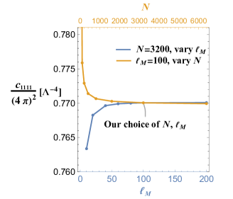
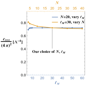
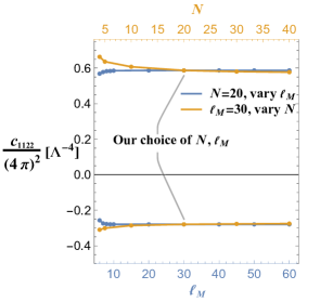
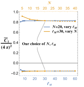
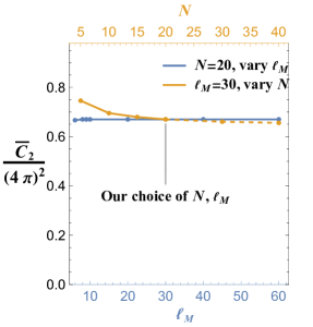
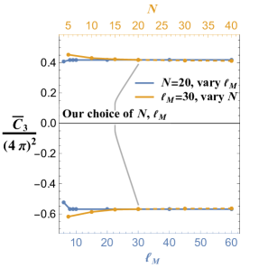
Figure 9: Convergence of the upper/lower bounds with respect to $N$ and $\ell_{M}$. Null constraints are used up to 3rd-order. The lines in the upper and lower half plane are the values of the upper and lower bounds, respectively, except for $c_{1111}$, $c_{1212}$ and $C_{2}$ where only the upper bounds are presented since their lower bounds are exactly zero.

Appendix E Numerical implementation and convergence

• Some numerical treatments
When performing the LP numerically, we rotate and rescale the decision variables to speed up the runs. For example, consider the unitarity condition $\big{|}\rho^{1234}_{\ell,n}\big{|}\leq\text{$\tfrac{1}{4}$}-\big{|}\tfrac{1}{4}-R^{1212}_{\ell,n}\big{|}$, which actually defines a square geometrically. So if we can redefine

$$\mathcal{R}_{\ell,n}=\frac{R^{1212}_{\ell,n}+\rho^{1234}_{\ell,n}}{2},\quad\mathcal{S}_{\ell,n}=\frac{R^{1212}_{\ell,n}-\rho^{1234}_{\ell,n}}{2},$$ (183)

this condition takes the much simpler form

$$0\leq\mathcal{R}_{\ell,n}\leq\frac{1}{4},\quad 0\leq\mathcal{S}_{\ell,n}\leq\frac{1}{4}\,.$$ (184)

After discretization, a null constraint schematically takes the form of $\sum_{\ell,n}(n/N)^{r}Q(\ell)\rho^{ijkl}_{\ell,n}=0$, where $r\geq 3$ is an integer and $Q(\ell)$ is some polynomial in $\ell$. When summing to a large $\ell$ and $n$, we see that the coefficients in the sum differ significantly in values, which slows down the numerical evaluation. To mitigate this problem, we can absorb certain powers of $\ell$ and $n$ into the spectral densities $\rho^{ijkl}_{\ell,n}\rightarrow\ell^{\hskip 0.35002pt\alpha}n^{\beta}\rho^{ijkl}_{\ell,n}$, $\alpha,\beta$ being integers. We have observed that this enhances the speed of the LP by several times.

• Checking convergence
Figure 9 shows how the upper/lower positivity bounds change with respect to $N$ and $\ell_{M}$, using up to 3rd-order null constraints. We see that despite the ideal case being $N,\ell_{M}\rightarrow\infty$, our choice of finite $N$ and $\ell_{M}$ is a very good approximation. The difference caused by finite $\ell_{M}$ is found to be negligible, and further increasing $N$ will improve the bounds by a few percent, which however becomes time-consuming. For $C_{i}$, the cases of $N>20$ are found to be too time-consuming, so we use extrapolation to get the bounds for larger $N$’s (shown as dashed lines in Figure 9). Specifically, we assume that the deviation from the true value goes like $\delta\propto 1/N$, which is true for $c_{1111}$, $c_{1212}$ and $c_{1122}$ and is consistent with the fact that the objective function is a discretized integration in the form of Eq. (30). This convergence study justifies our discretization scheme used in Section 2.3.

References

- (1) A. Adams, N. Arkani-Hamed, S. Dubovsky, A. Nicolis and R. Rattazzi, Causality, analyticity and an IR obstruction to UV completion, JHEP 10 (2006) 014, [hep-th/0602178].
- (2) C. de Rham, S. Melville, A. J. Tolley and S.-Y. Zhou, Positivity bounds for scalar field theories, Phys. Rev. D 96 (2017) 081702, [1702.06134].
- (3) C. de Rham, S. Melville, A. J. Tolley and S.-Y. Zhou, UV complete me: Positivity Bounds for Particles with Spin, JHEP 03 (2018) 011, [1706.02712].
- (4) N. Arkani-Hamed, T.-C. Huang and Y.-t. Huang, The EFT-Hedron, JHEP 05 (2021) 259, [2012.15849].
- (5) B. Bellazzini, J. Elias Miró, R. Rattazzi, M. Riembau and F. Riva, Positive moments for scattering amplitudes, Phys. Rev. D 104 (2021) 036006, [2011.00037].
- (6) A. J. Tolley, Z.-Y. Wang and S.-Y. Zhou, New positivity bounds from full crossing symmetry, JHEP 05 (2021) 255, [2011.02400].
- (7) S. Caron-Huot and V. Van Duong, Extremal Effective Field Theories, JHEP 05 (2021) 280, [2011.02957].
- (8) L.-Y. Chiang, Y.-t. Huang, W. Li, L. Rodina and H.-C. Weng, Into the EFThedron and UV constraints from IR consistency, JHEP 03 (2022) 063, [2105.02862].
- (9) A. Sinha and A. Zahed, Crossing Symmetric Dispersion Relations in Quantum Field Theories, Phys. Rev. Lett. 126 (2021) 181601, [2012.04877].
- (10) C. Zhang and S.-Y. Zhou, Convex Geometry Perspective on the (Standard Model) Effective Field Theory Space, Phys. Rev. Lett. 125 (2020) 201601, [2005.03047].
- (11) X. Li, H. Xu, C. Yang, C. Zhang and S.-Y. Zhou, Positivity in Multifield Effective Field Theories, Phys. Rev. Lett. 127 (2021) 121601, [2101.01191].
- (12) B. Bellazzini, L. Martucci and R. Torre, Symmetries, Sum Rules and Constraints on Effective Field Theories, JHEP 09 (2014) 100, [1405.2960].
- (13) B. Bellazzini, Softness and amplitudes’ positivity for spinning particles, JHEP 02 (2017) 034, [1605.06111].
- (14) Z. Bern, D. Kosmopoulos and A. Zhiboedov, Gravitational effective field theory islands, low-spin dominance, and the four-graviton amplitude, J. Phys. A 54 (2021) 344002, [2103.12728].
- (15) L. Alberte, C. de Rham, S. Jaitly and A. J. Tolley, Positivity Bounds and the Massless Spin-2 Pole, Phys. Rev. D 102 (2020) 125023, [2007.12667].
- (16) J. Tokuda, K. Aoki and S. Hirano, Gravitational positivity bounds, JHEP 11 (2020) 054, [2007.15009].
- (17) S. Caron-Huot, D. Mazac, L. Rastelli and D. Simmons-Duffin, Sharp boundaries for the swampland, JHEP 07 (2021) 110, [2102.08951].
- (18) A. Guerrieri and A. Sever, Rigorous Bounds on the Analytic S Matrix, Phys. Rev. Lett. 127 (2021) 251601, [2106.10257].
- (19) Z.-Z. Du, C. Zhang and S.-Y. Zhou, Triple crossing positivity bounds for multi-field theories, JHEP 12 (2021) 115, [2111.01169].
- (20) L. Alberte, C. de Rham, S. Jaitly and A. J. Tolley, Reverse Bootstrapping: IR Lessons for UV Physics, Phys. Rev. Lett. 128 (2022) 051602, [2111.09226].
- (21) B. Bellazzini, M. Riembau and F. Riva, IR side of positivity bounds, Phys. Rev. D 106 (2022) 105008, [2112.12561].
- (22) L.-Y. Chiang, Y.-t. Huang, L. Rodina and H.-C. Weng, De-projecting the EFThedron, 2204.07140.
- (23) S. Caron-Huot, Y.-Z. Li, J. Parra-Martinez and D. Simmons-Duffin, Causality constraints on corrections to Einstein gravity, JHEP 05 (2023) 122, [2201.06602].
- (24) L.-Y. Chiang, Y.-t. Huang, W. Li, L. Rodina and H.-C. Weng, (Non)-projective bounds on gravitational EFT, 2201.07177.
- (25) M. Carrillo González, C. de Rham, S. Jaitly, V. Pozsgay and A. Tokareva, Positivity-causality competition: a road to ultimate EFT consistency constraints, 2307.04784.
- (26) D.-Y. Hong, Z.-H. Wang and S.-Y. Zhou, Causality bounds on scalar-tensor EFTs, 2304.01259.
- (27) C. de Rham, S. Kundu, M. Reece, A. J. Tolley and S.-Y. Zhou, Snowmass White Paper: UV Constraints on IR Physics, in Snowmass 2021, 3, 2022. 2203.06805.
- (28) C. Zhang and S.-Y. Zhou, Positivity bounds on vector boson scattering at the LHC, Phys. Rev. D 100 (2019) 095003, [1808.00010].
- (29) Q. Bi, C. Zhang and S.-Y. Zhou, Positivity constraints on aQGC: carving out the physical parameter space, JHEP 06 (2019) 137, [1902.08977].
- (30) B. Bellazzini and F. Riva, New phenomenological and theoretical perspective on anomalous ZZ and Z processes, Phys. Rev. D 98 (2018) 095021, [1806.09640].
- (31) G. N. Remmen and N. L. Rodd, Consistency of the Standard Model Effective Field Theory, JHEP 12 (2019) 032, [1908.09845].
- (32) K. Yamashita, C. Zhang and S.-Y. Zhou, Elastic positivity vs extremal positivity bounds in SMEFT: a case study in transversal electroweak gauge-boson scatterings, JHEP 01 (2021) 095, [2009.04490].
- (33) T. Trott, Causality, unitarity and symmetry in effective field theory, JHEP 07 (2021) 143, [2011.10058].
- (34) G. N. Remmen and N. L. Rodd, Flavor Constraints from Unitarity and Analyticity, Phys. Rev. Lett. 125 (2020) 081601, [2004.02885].
- (35) G. N. Remmen and N. L. Rodd, Signs, spin, SMEFT: Sum rules at dimension six, Phys. Rev. D 105 (2022) 036006, [2010.04723].
- (36) J. Gu and L.-T. Wang, Sum Rules in the Standard Model Effective Field Theory from Helicity Amplitudes, JHEP 03 (2021) 149, [2008.07551].
- (37) B. Fuks, Y. Liu, C. Zhang and S.-Y. Zhou, Positivity in electron-positron scattering: testing the axiomatic quantum field theory principles and probing the existence of UV states, Chin. Phys. C 45 (2021) 023108, [2009.02212].
- (38) J. Gu, L.-T. Wang and C. Zhang, Unambiguously Testing Positivity at Lepton Colliders, Phys. Rev. Lett. 129 (2022) 011805, [2011.03055].
- (39) Q. Bonnefoy, E. Gendy and C. Grojean, Positivity bounds on Minimal Flavor Violation, JHEP 04 (2021) 115, [2011.12855].
- (40) J. Davighi, S. Melville and T. You, Natural selection rules: new positivity bounds for massive spinning particles, JHEP 02 (2022) 167, [2108.06334].
- (41) M. Chala and J. Santiago, Positivity bounds in the standard model effective field theory beyond tree level, Phys. Rev. D 105 (2022) L111901, [2110.01624].
- (42) C. Zhang, SMEFTs living on the edge: determining the UV theories from positivity and extremality, JHEP 12 (2022) 096, [2112.11665].
- (43) D. Ghosh, R. Sharma and F. Ullah, Amplitude’s positivity vs. subluminality: causality and unitarity constraints on dimension 6 & 8 gluonic operators in the SMEFT, JHEP 02 (2023) 199, [2211.01322].
- (44) G. N. Remmen and N. L. Rodd, Spinning sum rules for the dimension-six SMEFT, JHEP 09 (2022) 030, [2206.13524].
- (45) X. Li and S. Zhou, Origin of neutrino masses on the convex cone of positivity bounds, Phys. Rev. D 107 (2023) L031902, [2202.12907].
- (46) X. Li, K. Mimasu, K. Yamashita, C. Yang, C. Zhang and S.-Y. Zhou, Moments for positivity: using Drell-Yan data to test positivity bounds and reverse-engineer new physics, JHEP 10 (2022) 107, [2204.13121].
- (47) X. Li, Positivity bounds at one-loop level: the Higgs sector, JHEP 05 (2023) 230, [2212.12227].
- (48) W. Altmannshofer, S. Gori, B. V. Lehmann and J. Zuo, UV physics from IR features: New prospects from top flavor violation, Phys. Rev. D 107 (2023) 095025, [2303.00781].
- (49) J. Davighi, S. Melville, K. Mimasu and T. You, Positivity and the Electroweak Hierarchy, 2308.06226.
- (50) L. Lehman and A. Martin, Low-derivative operators of the Standard Model effective field theory via Hilbert series methods, JHEP 02 (2016) 081, [1510.00372].
- (51) B. Henning, X. Lu, T. Melia and H. Murayama, 2, 84, 30, 993, 560, 15456, 11962, 261485, …: Higher dimension operators in the SM EFT, JHEP 08 (2017) 016, [1512.03433].
- (52) L. Vecchi, Causal versus analytic constraints on anomalous quartic gauge couplings, JHEP 11 (2007) 054, [0704.1900].
- (53) M. F. Paulos, J. Penedones, J. Toledo, B. C. van Rees and P. Vieira, The S-matrix bootstrap. Part III: higher dimensional amplitudes, JHEP 12 (2019) 040, [1708.06765].
- (54) A. L. Guerrieri, J. Penedones and P. Vieira, S-matrix bootstrap for effective field theories: massless pions, JHEP 06 (2021) 088, [2011.02802].
- (55) A. Guerrieri, J. Penedones and P. Vieira, Where Is String Theory in the Space of Scattering Amplitudes?, Phys. Rev. Lett. 127 (2021) 081601, [2102.02847].
- (56) J. Elias Miro, A. Guerrieri and M. A. Gumus, Bridging positivity and S-matrix bootstrap bounds, JHEP 05 (2023) 001, [2210.01502].
- (57) K. Häring, A. Hebbar, D. Karateev, M. Meineri and J. a. Penedones, Bounds on photon scattering, 2211.05795.
- (58) M. Kruczenski, J. Penedones and B. C. van Rees, Snowmass White Paper: S-matrix Bootstrap, 2203.02421.
- (59) H. Xu and S.-Y. Zhou, Triple crossing positivity bounds, mass dependence and cosmological scalars: Horndeski theory and DHOST, 2306.06639.
- (60) D. Poland, S. Rychkov and A. Vichi, The Conformal Bootstrap: Theory, Numerical Techniques, and Applications, Rev. Mod. Phys. 91 (2019) 015002, [1805.04405].
- (61) M. Froissart, Asymptotic behavior and subtractions in the Mandelstam representation, Phys. Rev. 123 (1961) 1053–1057.
- (62) A. Martin, Unitarity and high-energy behavior of scattering amplitudes, Phys. Rev. 129 (1963) 1432–1436.
- (63) C. de Rham, S. Melville, A. J. Tolley and S.-Y. Zhou, Massive Galileon Positivity Bounds, JHEP 09 (2017) 072, [1702.08577].
- (64) A. V. Manohar, Introduction to Effective Field Theories, 1804.05863.
- (65) O. J. P. Eboli, M. C. Gonzalez-Garcia and J. K. Mizukoshi, p p — j j e+- mu+- nu nu and j j e+- mu-+ nu nu at O( alpha(em)**6) and O(alpha(em)**4 alpha(s)**2) for the study of the quartic electroweak gauge boson vertex at CERN LHC, Phys. Rev. D 74 (2006) 073005, [hep-ph/0606118].
- (66) E. d. S. Almeida, O. J. P. Éboli and M. C. Gonzalez–Garcia, Unitarity constraints on anomalous quartic couplings, Phys. Rev. D 101 (2020) 113003, [2004.05174].
- (67) H.-L. Li, Z. Ren, J. Shu, M.-L. Xiao, J.-H. Yu and Y.-H. Zheng, Complete set of dimension-eight operators in the standard model effective field theory, Phys. Rev. D 104 (2021) 015026, [2005.00008].
- (68) C. W. Murphy, Dimension-8 operators in the Standard Model Eective Field Theory, JHEP 10 (2020) 174, [2005.00059].
- (69) CMS collaboration, A. M. Sirunyan et al., Observation of electroweak production of same-sign W boson pairs in the two jet and two same-sign lepton final state in proton-proton collisions at 13 TeV, Phys. Rev. Lett. 120 (2018) 081801, [1709.05822].
- (70) ATLAS collaboration, M. Aaboud et al., Observation of electroweak production of a same-sign boson pair in association with two jets in collisions at TeV with the ATLAS detector, Phys. Rev. Lett. 123 (2019) 161801, [1906.03203].
- (71) J.-C. Yang, Z.-B. Qing, X.-Y. Han, Y.-C. Guo and T. Li, Tri-photon at muon collider: a new process to probe the anomalous quartic gauge couplings, JHEP 22 (2020) 053, [2204.08195].
- (72) J.-C. Yang, Y.-C. Guo, C.-X. Yue and Q. Fu, Constraints on anomalous quartic gauge couplings via Zjj production at the LHC, Phys. Rev. D 104 (2021) 035015, [2107.01123].
- (73) R. Gomez-Ambrosio, Studies of Dimension-Six EFT effects in Vector Boson Scattering, Eur. Phys. J. C 79 (2019) 389, [1809.04189].
- (74) J. J. Ethier, R. Gomez-Ambrosio, G. Magni and J. Rojo, SMEFT analysis of vector boson scattering and diboson data from the LHC Run II, Eur. Phys. J. C 81 (2021) 560, [2101.03180].
- (75) C. Degrande, A basis of dimension-eight operators for anomalous neutral triple gauge boson interactions, JHEP 02 (2014) 101, [1308.6323].
- (76) A. Senol, H. Denizli, A. Yilmaz, I. Turk Cakir, K. Y. Oyulmaz, O. Karadeniz et al., Probing the Effects of Dimension-eight Operators Describing Anomalous Neutral Triple Gauge Boson Interactions at FCC-hh, Nucl. Phys. B 935 (2018) 365–376, [1805.03475].
- (77) R. Rahaman and R. K. Singh, Anomalous triple gauge boson couplings in production at the LHC and the role of boson polarizations, Nucl. Phys. B 948 (2019) 114754, [1810.11657].
- (78) A. Senol, H. Denizli, A. Yilmaz, I. Turk Cakir and O. Cakir, Study on Anomalous Neutral Triple Gauge Boson Couplings from Dimension-eight Operators at the HL-LHC, 1906.04589.
- (79) J. Ellis, S.-F. Ge, H.-J. He and R.-Q. Xiao, Probing the scale of new physics in the coupling at colliders, Chin. Phys. C 44 (2020) 063106, [1902.06631].
- (80) J. Ellis, H.-J. He and R.-Q. Xiao, Probing new physics in dimension-8 neutral gauge couplings at e+e- colliders, Sci. China Phys. Mech. Astron. 64 (2021) 221062, [2008.04298].
- (81) Q. Fu, J.-C. Yang, C.-X. Yue and Y.-C. Guo, The study of neutral triple gauge couplings in the process e+e→Z including unitarity bounds, Nucl. Phys. B 972 (2021) 115543, [2102.03623].
- (82) D. Lombardi, M. Wiesemann and G. Zanderighi, Anomalous couplings in Z events at NNLO+PS and improving ¯ backgrounds in dark-matter searches, Phys. Lett. B 824 (2022) 136846, [2108.11315].
- (83) S. Jahedi and J. Lahiri, Probing anomalous ZZ and Z couplings at the e+e- colliders using optimal observable technique, JHEP 04 (2023) 085, [2212.05121].
- (84) A. Senol, S. Spor, E. Gurkanli, V. Cetinkaya, H. Denizli and M. Köksal, Model-independent study on the anomalous and couplings at the future muon collider, Eur. Phys. J. Plus 137 (2022) 1354, [2205.02912].
- (85) J. Ellis, H.-J. He and R.-Q. Xiao, Probing neutral triple gauge couplings at the LHC and future hadron colliders, Phys. Rev. D 107 (2023) 035005, [2206.11676].
- (86) S. Spor, E. Gurkanli and M. Köksal, Search for the anomalous ZZ and Z couplings via production at the CLIC, Nucl. Phys. B 979 (2022) 115785, [2203.02352].
- (87) C. Degrande and H.-L. Li, Impact of dimension-8 SMEFT operators on diboson productions, JHEP 06 (2023) 149, [2303.10493].
- (88) C. H. Llewellyn Smith, High-Energy Behavior and Gauge Symmetry, Phys. Lett. B 46 (1973) 233–236.
- (89) B. W. Lee, C. Quigg and H. B. Thacker, Weak Interactions at Very High-Energies: The Role of the Higgs Boson Mass, Phys. Rev. D 16 (1977) 1519.
- (90) B. W. Lee, C. Quigg and H. B. Thacker, The Strength of Weak Interactions at Very High-Energies and the Higgs Boson Mass, Phys. Rev. Lett. 38 (1977) 883–885.
- (91) J. M. Cornwall, D. N. Levin and G. Tiktopoulos, Derivation of Gauge Invariance from High-Energy Unitarity Bounds on the s Matrix, Phys. Rev. D 10 (1974) 1145.
- (92) O. J. P. Éboli and M. C. Gonzalez-Garcia, Classifying the bosonic quartic couplings, Phys. Rev. D 93 (2016) 093013, [1604.03555].
- (93) CMS collaboration, A. M. Sirunyan et al., Search for anomalous electroweak production of vector boson pairs in association with two jets in proton-proton collisions at 13 TeV, Phys. Lett. B 798 (2019) 134985, [1905.07445].
- (94) A. Cappati, R. Covarelli, P. Torrielli and M. Zaro, Sensitivity to new physics in final states with multiple gauge and Higgs bosons, JHEP 09 (2022) 038, [2205.15959].
- (95) M. Soldate, Partial Wave Unitarity and Closed String Amplitudes, Phys. Lett. B 186 (1987) 321–327.