2D hydrodynamic electron flow through periodic and random potentials

Abstract

We study the hydrodynamic flow of electrons through a smooth potential energy landscape in two dimensions, for which the electrical current is concentrated along thin channels that follow percolating equipotential contours. The width of these channels, and hence the electrical resistance, is determined by a competition between viscous and thermoelectric forces. For the case of periodic (moiré) potentials, we find that hydrodynamic flow provides a new route to linear-in-$T$ resistivity. We calculate the associated prefactors for potentials with $C_{3}$ and $C_{4}$ symmetry. On the other hand, for a random potential the resistivity has qualitatively different behavior because equipotential paths become increasingly tortuous as their width is reduced. This effect leads to a resistivity that grows with temperature as $T^{10/3}$.

Introduction – Under conditions where electrons collide much more frequently with one another than with anything else, the current carried by an electron system flows like a fluid rather than satisfying the usual Ohm’s law. This hydrodynamic electron regime was described by Gurzhi in the 1960s [1, 2], and it has attracted significant attention during the last decade owing largely to its realization in graphene [3, 4, 5, 6, 7, 8, 9, 10, 11, 12, 13, 14, 15, 16, 17, 18, 19, 20, 21, 22, 23, 24, 25, 26, 27, 28, 29, 30, 31, 32, 33, 34, 35]. Recent experiments have demonstrated a variety of transport phenomena associated with hydrodynamic electrons, including negative non-local resistance [8, 9, 13, 14, 27, 36, 15], Pouiselle-like flow profiles [18, 19, 20, 21, 22, 28, 37], superballistic flow [11, 12], Wiedemann-Franz law violations [38, 39, 40, 10, 41, 25, 42, 43, 44, 45, 46, 47, 48], and bulk field expulsion [29, 30, 31].

Where disorder effects are included in descriptions of hydrodynamic electron flow, these effects are usually implemented via a finite momentum relaxation rate. Such a description is equivalent to imagining spatially uncorrelated, delta-function scatterers. On the other hand, in Ref. [49] Andreev, Kivelson, and Spivak (AKS) considered hydrodynamic electron flow through a smooth random potential that varies on a length scale that is long compared to the electron-electron mean free path $\ell_{ee}$. AKS considered two contributions to the electrical resistance in this setting, arising from viscous shear stresses and thermoelectric fields. Using an “energy minimization” argument (properly, entropy maximization, as we explain below), they argued that when the electronic viscosity or thermal conductivity is low enough, the electric current in two dimensions is concentrated along narrow channels that follow equipotential contours, as sketched in Fig. 1. AKS derived a corresponding result for the resistivity (up to numeric prefactors).

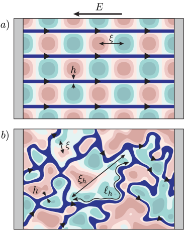
Figure 1: A device sketch with the imposed external potential $U$ (blue and red contour lines), where the shaded dark blue lines correspond to current flow under the applied electric field $E$. The thin current channels of width $h$ are concentrated about equipotential contours of $U$. a) The case of square periodic potential $U=U_{0}\cos(2\pi x/\xi)\cos(2\pi y/\xi)$. b) The case of a random potential, for which the equipotential contours and the current channels meander and become tortuous in nature, controlled by the hull correlation length $\xi_{h}$ and the hull perimeter $\ell_{h}$.

In this paper, we reconsider the problem of hydrodynamic flow through a smooth potential and provide two important updates to the AKS result. First, we consider the flow through a periodic (moiré) potential. We derive the corresponding resistivity, which follows the same form as the AKS result, and we give appropriate numeric prefactors for periodic potentials with $C_{3}$ and $C_{4}$ symmetry. We further show that, for electron systems obeying Fermi liquid theory, the result implies a linear-in-$T$ dependence of the resistance.

These results may have a direct connection to recent transport experiments. Strong, slowly-varying periodic potentials now abound experimentally due to the explosion of interest in moiré systems [50, 51, 52, 53, 54, 55, 56, 57, 58, 59, 60, 61, 62]. In both twisted bilayer graphene [63] and TMD (transition metal dichalcogenide) systems [64, 65], regimes of linear-in-$T$ resistivity have been experimentally discovered near strongly correlated phases. As both pedestrian explanations and exotic conjectures have been put forth for this temperature dependence [66, 67, 68, 69, 70], it is important that we understand all possible routes to linear-in-$T$ resistivity.

Second, we turn our attention to the case of a spatially random potential. We show that the AKS result no longer applies because current-carrying channels become increasingly tortuous as their width decreases. Instead, the resistivity is governed by nontrivial critical exponents associated with two-dimensional (2D) percolation, leading to a superlinear $T^{10/3}$ dependence of the resistivity on temperature. We conclude with some brief remarks on how both results may be tested experimentally.

Mathematical Setup – The hydrodynamic equations that govern viscous electron flow are

$$-\nabla P-en\mathbf{E}-\nabla U_{\text{dis}}-mn\nu\nabla\times\nabla\times\mathbf{v}$$

$$\phantom{-\nabla P}+mn\left[\frac{D-1}{D}2\nu+\tilde{\zeta}\right]\nabla\nabla\cdot\mathbf{v}=mn\mathbf{v}\cdot\nabla\mathbf{v}$$ (1)

$$\kappa\nabla^{2}T+\frac{1}{2}mn\nu\left(\partial_{i}v_{j}+\partial_{j}v_{i}-\frac{2}{D}\delta_{ij}\partial_{k}v_{k}\right)^{2}$$

$$\phantom{\kappa\nabla^{2}T+\frac{1}{2}mn\nu\Big{(}\partial_{i}v_{j}}+mn\tilde{\zeta}(\nabla\cdot\mathbf{v})^{2}=mnT\mathbf{v}\cdot\nabla s$$ (2)

$$\nabla\cdot(n\mathbf{v})=0,$$ (3)

where $m$ is the hydrodynamic mass, $-e$ is the electron charge, and $D=2$ is the dimensionality. The hydrodynamic variables are the velocity $\mathbf{v}$, the pressure $P$, the particle density $n$. We treat the electric field $\mathbf{E}$ as a weak, externally applied field. Eq. (2D hydrodynamic electron flow through periodic and random potentials) is the Navier-Stokes (momentum) equation, with kinematic shear viscosity $\nu$ and kinematic bulk viscosity $\tilde{\zeta}$, as well as the externally imposed disorder potential $U_{\text{dis}}$. Eq. (2D hydrodynamic electron flow through periodic and random potentials) is the heat (energy) equation, with thermal conductivity $\kappa$ and entropy per unit mass $s$. Finally, Eq. (3) is the density continuity equation. To complete the set of equations, we need constitutive relations between our hydrodynamic variables. Since $(s,T)$ and $(n,P)$ are thermodynamically conjugate variables, we choose one from each set to be our independent variables. In particular, we choose variables $n$ and $T$ so that

$$\nabla P(n,T)= \frac{\partial P}{\partial n}\nabla n-mn^{2}\frac{\partial s}{\partial n}\nabla T$$ (4)

$$\nabla s(n,T)= \frac{\partial s}{\partial n}\nabla n+\frac{\partial s}{\partial T}\nabla T$$ (5)

where $n_{s}\equiv mns$ is the entropy density and we used the thermodynamic relation $(\partial P/\partial T)=-mn^{2}(\partial s/\partial n)$. For simplicity, we assume that $\partial P/\partial n>0$ and $\partial s/\partial n<0$ are constants. Finally, we consider a rectangular domain $[0,L_{x}]\times[0,L_{y}]$ as shown in Fig. 1. For boundary conditions (BCs), we fix $T=\overline{T}$ and take periodic BCs for $n$ on the $x$-boundaries. Furthermore, we take for simplicity periodic BCs on the $y$-boundaries .

We are interested in the linear-response theory of the above equations without assuming that $\nabla U_{\text{dis}}$ is weak. Therefore, we look to organize our solution in a formal perturbative scheme $\mathbf{v}=\mathbf{v}^{(0)}+\mathbf{v}^{(1)}+\ldots$, and similarly for the other hydrodynamic variables. We will determine the explicit perturbative parameter ex post facto. At leading (zeroth) order, we consider the equilibrium situation where we expect $\mathbf{v}^{(0)}=0$ and $T^{(0)}=\overline{T}$. Therefore, the only non-trivial equation at zeroth order is

$$-\nabla P^{(0)}-\nabla U_{\text{dis}}=0$$ (6)

where we have kept $U_{\text{dis}}$ since it is not perturbatively small. From the constitutive relations, this implies that $\nabla n^{(0)}\propto\nabla U_{\text{dis}}\propto\nabla s^{(0)}$. Thus, the density and entropy per mass profiles are inherited from the disorder potential at leading order.

We now consider the first-order hydrodynamic equations, driven by a perturbatively weak field $\mathbf{E}$. These are given by the equations

$$-\nabla P^{(1)}-en^{(0)}\mathbf{E}-mn^{(0)}\nu\nabla\times\nabla\times\mathbf{v}^{(1)}$$

$$\phantom{-\nabla P^{(0)}}+mn^{(0)}\left[\frac{D-1}{D}2\nu+\tilde{\zeta}\right]\nabla\nabla\cdot\mathbf{v}^{(1)}=0$$ (7)

$$\kappa\nabla^{2}T^{(1)}=mn^{(0)}\overline{T}\mathbf{v}^{(1)}\cdot\nabla s^{(0)}$$ (8)

$$\nabla\cdot(n^{(0)}\mathbf{v}^{(1)})=0,$$ (9)

where we treat $\mathbf{E}$ as a first-order perturbation. Eqs. (7) – (9) are equivalent to those in Ref. 49, with the perturbation theory considerations manifestly written. It is crucial that one utilizes the temperature-dependence in Eq. (4); otherwise, Eq. (7) decouples from Eq. (8). This dependence provides a “thermoelectric” contribution to Eq. (7), which is the key term in restricting current to flow along narrow channels .

A convenient way to obtain the two-terminal resistance $R$ is to compute the total entropy generation. The relation between these two quantities is subtle, and proceeds as follows. One can show that the entropy production of a hydrodynamic system is given by [73]

$$\int dV\frac{dn_{s}}{dt}=-\oint\left(n_{s}\mathbf{v}+\frac{\kappa\nabla T}{T}\right)\cdot d\mathbf{A}+\int dV\frac{q}{T}$$ (10)

with

$$q\equiv\frac{1}{T}\kappa(\nabla T)^{2}+\frac{1}{2}mn\nu\left(\partial_{i}v_{j}+\partial_{j}v_{i}-\frac{2}{D}\delta_{ik}\partial_{l}v_{l}\right)^{2}$$

$$\phantom{q=\frac{1}{T}\kappa(\nabla T)^{2}}+mn\tilde{\zeta}(\nabla\cdot\mathbf{v})^{2}.$$ (11)

Note that $q/T$ is positive semi-definite and can therefore be interpreted as the bulk entropy production. In steady-state the LHS of Eq. (10) vanishes, and thus all the bulk-generated entropy flows out through the contacts held at $\overline{T}$. On physical grounds, we assume that this entropy outflow is gained as heat by the environment through the contacts at temperature $\overline{T}$. Thus, by equating the dissipated $I^{2}R$ power to the environmental heating, we have

$$I^{2}R =\overline{T}\int dV\frac{q}{T}$$ (12)

When the variations of $T$ are small such that $T\approx\overline{T}$, we have the simpler relation $I^{2}R=\int dVq$ as written by Ref. [49]. Only in this limit of $\delta T\ll\bar{T}$ can one interpret Eq. (12) as energy conservation with $q$ as the “local power dissipation” . Throughout this paper, we make the assumption $\delta T\simeq T^{(1)}\ll\overline{T}$ and therefore use the simpler relation.

Periodic Potential – Using Eqs. (11) and (12), we calculate the resistance for different cases of the disorder potential. Let us first consider the case of a square periodic potential ${U_{\text{dis, sq}}=U_{0}\cos(2\pi x/\xi)\cos(2\pi y/\xi)}$ with periodicity $\xi$ (see Fig. 1a); this case was sketched by Ref. 49. As we argued above, the zeroth order density $n^{(0)}$ and entropy density $s^{(0)}$ also fluctuate around their mean values with the same spatial periodicity. In the strong disorder limit, we make the ansatz that the flow is isolated to thin horizontal channels of width $h$ and length $\ell=L_{x}$, centered around the equipotential lines of $s^{(0)}=\overline{s}$ (see Fig. 1a). Each of the $N=L_{y}/\xi$ such channels carries an equal amount of current $I/N$, where $I$ is the total current. We further assume that the flow is incompressible, i.e. that $\nabla\cdot\mathbf{v}=0$. This incompressibility assumption is justified if $(n^{(0)}-\overline{n})\ll\overline{n}$ within the channel ; we show below that this assumption is valid for $h/\xi\ll 1$. Finally, we assume that the temperature fluctuations outside of the channel are negligible, since the dominant heating is isolated to within the thin channels.

Assuming that the flow chooses an optimum channel width $h$ to minimize the total dissipated power, we estimate the power dissipation. Implicit in this assumption is that the heat current influences flow, e.g. through a thermoelectric term. In the incompressible limit, the leading order contribution to dissipation is

$$I^{2}R=N\int_{\text{ch}}dV\frac{1}{T_{0}}\kappa\left(\nabla T^{(1)}\right)^{2}+\frac{m\overline{n}\nu}{2}\left(\partial_{i}v_{j}^{(1)}+\partial_{j}v_{i}^{(1)}\right)^{2},$$ (13)

where the integral is over a single channel and we can approximate $n^{(0)}\sim\overline{n}$. By a scaling estimate similar to the one in Ref. [49], we find

$$I^{2}R\sim\frac{I^{2}}{Ne^{2}}\frac{\ell}{\xi}\left[\frac{\overline{T}}{\kappa}(m\overline{\delta s})^{2}\left(\frac{h}{\xi}\right)^{3}+\frac{m\nu}{\overline{n}\xi^{2}}\left(\frac{\xi}{h}\right)^{3}\right]$$ (14)

where $\overline{\delta{s}}$ is the characteristic amplitude of the entropy fluctuations and we have used Eq. (8) and the approximations $h\ll\xi$, $v_{y}\ll v_{x}$, $\partial_{x}\sim 1/\xi$, and ${\partial_{y}\sim 1/h}$. From Eq. (14) one can see that there are two resistance contributions which compete in determining the channel width $h$. The first term, corresponding to dissipation from thermoelectrically-driven heat currents, favors narrow channels. The second term, corresponding to dissipation from viscous shearing, favors wide channels. Minimizing the dissipated power against $h$, we find that

$$\frac{h}{\xi}\sim\left(\frac{\overline{T}\overline{\delta n_{s}}^{2}\xi^{2}}{\kappa\eta}\right)^{-1/6}\equiv\alpha^{-1/6}$$ (15)

where $\overline{\delta n_{s}}=m\overline{n}\overline{\delta s}$ is the characteristic strength of entropy density fluctuations and $\eta=m\overline{n}\nu$ is the dynamic viscosity. Therefore, we find perturbative control when $(\xi/h)^{6}\sim\alpha\gg 1$ (when channels are narrow). Furthermore, we need to ensure that the thermoelectric term in Eq. (4) is sufficiently large to ensure that channels actually form. A perturbative solution around $\partial s/\partial n=0$ does not form channels; since Eq. (8) decouples in this limit, the solution has non-zero velocity everywhere with velocity variations set by $\xi$ from the continuity equation [Eq. (9)]. Via a scaling estimate, this perturbative ansatz fails when ${(\overline{n}/\overline{\delta s})|\partial s/\partial n|\alpha\gg 1}$. Finally, our incompressibility assumption is valid if $(\overline{\delta n}/\overline{n})\alpha^{-1/6}\ll 1$ for $\overline{\delta{n}}$ the characteristic strength of density fluctuations. Thus, all our assumptions are controlled by $\alpha\gg 1$ up to dimensionless factors.

Plugging Eq. (15) into Eq. (14), we find the resistivity to be

$$\rho\sim\frac{2}{e^{2}}\sqrt{\frac{\overline{T}\eta(m\overline{\delta s})^{2}}{\kappa\overline{n}^{2}\xi^{2}}}$$ (16)

This equation recovers the results of Ref. 49. Below we numerically verify these results and determine the proportionality coefficient [see Eq. (21)]. For a Fermi liquid, Eq. (16) implies a particular temperature dependence of the resistance. Specifically, a Fermi liquid has viscosity $\eta\sim T^{-2}$, thermal conductivity $\kappa\sim T^{-1}$, and entropy density $\overline{\delta n_{s}}\sim T$ [49]. These substitutions give $h\propto 1/T$ and we find a linear $\rho\propto T$ scaling, as mentioned above.

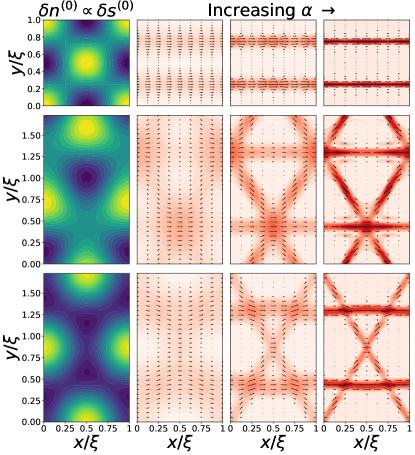
Figure 2: Numerical solutions for the current density $\mathbf{j}$ in various periodic potentials. Each row corresponds to a particular type of potential, illustrated in the first column (top to bottom: square potential, triangular potential with $\psi=\pi/6$, triangular potential with $\psi=0$). Columns 2-4 show the simulated current density (arrows show direction and color darkness shows magnitude) for each potential. Columns 2-4 correspond to $\alpha\sim 10^{3},10^{5},$ and $10^{7}$, respectively. As $\alpha$ increases, the current-carrying channels become increasingly narrow.

Numerical Simulation – For the case of periodic potentials, we can provide direct numerical solutions of the hydrodynamic equations to verify our scaling results. Specifically, we solve Eqs. (7) – (9) with the above BCs using the spectral PDE solver Dedalus [77]. We emphasize that for these simulations we make no assumptions about $n^{(0)}$ and in particular do not assume incompressibility. For simplicity, we assume the bulk viscosity $\tilde{\zeta}=0$ in our simulations; numerically tuning this parameter has little effect on the qualitative flow profile. This irrelevance of $\tilde{\zeta}$ is as expected, since we expect flow to be approximately incompressible when thin channels form. In addition to the square potential, we consider a class of triangular potentials that describe the moiré pattern arising from mismatched hexagonal lattices (as in graphene or transition metal dichalcogenides) [78]. Such potentials have one free parameter, $\psi$, that describes the phase difference between the moiré reciprocal lattice vectors (see Appendix for details). The results of these numerical simulations are shown in Fig. 2 for a range of values of $\alpha$. We observe the formation of current-carrying channels along the equipotential contours that span the system. Furthermore, the channels become increasingly narrow as $\alpha$ is increased, as predicted.

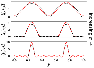
Figure 3: Numerical results for the averaged current density profile $\langle j_{x}\rangle_{x}\equiv\int dxj_{x}/L_{x}$ in a square-periodic potential, normalized by total current $I$. The three values of $\alpha$ are the same as those in Fig. 2. The solid lines correspond to the results of direct numerical simulation, while dashed lines correspond to our approximate variational solution.

In order to provide a quantitative calculation of the resistance, we adopt a variational approach that assumes a parabolic flow profile within each channel. Specifically, we assume a current density $j_{x}(x,y)=6(I/N)[(h/2)^{2}-y^{2}]/h^{3}$ within each channel (with $y=0$ corresponding to the center of a given channel) and zero elsewhere. The width $h$ of the channel is treated as a variational parameter; see Fig. 3 for a comparison between our ansatz for $j_{x}(y)$ and exact numerical solutions. This ansatz for $\mathbf{j}=e\overline{n}\mathbf{v}$ yields a temperature $T^{(1)}$ via Eq. (8). Consequently, we arrive at analytic expressions for both of the power dissipation terms in Eq. (14), in the limit of $h\ll\xi$, with exact numerical prefactors for square and triangular potential profiles:

$$Q_{\text{th}} =C_{\text{th}}\frac{I^{2}L_{x}\overline{T}}{e^{2}L_{y}\kappa}(m\overline{\delta s})^{2}\left(\frac{h}{\xi}\right)^{3}$$ (17)

$$Q_{\text{vis}} =C_{\text{vis}}\frac{I^{2}L_{x}m\nu}{e^{2}L_{y}\overline{n}\xi^{2}}\left(\frac{\xi}{h}\right)^{3}$$ (18)

$$C_{\text{th, sq}} =\frac{\pi^{4}}{35} ,\>\>C_{\text{th, tri}} =\frac{4\pi^{4}}{630}$$ (19)

$$C_{\text{vis, sq}} =24 ,\>\>C_{\text{vis, tri}} =\frac{24}{\left(1-\frac{\overline{\delta n}}{\sqrt{6}\,n}\text{cos}(3\psi)\right)^{2}}$$ (20)

where $Q_{\text{th}}$ and $Q_{\text{vis}}$ correspond to the thermal (first) and viscous (second) terms in Eq. (14).

As before, we look for a channel width $h$ such that $Q_{\text{th}}+Q_{\text{vis}}$ is minimized. We plot the variational result for the current density in Fig. 3 along with the corresponding result from direct numerical simulation, which shows close agreement. Finally, we compute the resistivity by evaluating the total power with the variationally-determined channel width $h$. This procedure gives

$$\rho=\frac{C}{e^{2}}\frac{\overline{\delta n_{s}}}{\overline{n}^{2}\xi}\sqrt{\frac{\overline{T}\eta}{\kappa}}.$$ (21)

This result validates the scaling result of Eq. (16) up to the numerical prefactor $C$, which for square and triangular potentials are given by

$$C =4\pi^{2}\sqrt{\frac{6}{35}}$$ (square)

$$C =\frac{8\pi^{2}}{\sqrt{105}\left(1-\frac{\overline{\delta n}}{\sqrt{6}\,n}\text{cos}(3\psi)\right)}$$ (triangular)

(see Appendix for details).

Random Potential – We now turn our attention to the case of a smooth random potential with a correlation length $\xi$ . Such random potentials arise, for example, from charged impurities in the substrate or an adjacent delta-doping layer, for which that the typical wave vector of the disorder potential is much smaller than the electron wave vector (see, e.g., Ref. [80] and references therein). This consideration is distinct from a model of point defect scatters studied in, e.g., Ref. [81].

The key conceptual novelty of a random potential is that equipotential lines are very tortuous [82], and therefore so are the current-carrying channels (see Fig. 1b). In particular, the number of parallel current-carrying channels $N$ and the contour length $\ell$ of each channel now depend on percolation exponents. In 2D, the hull correlation length exponent is $\nu_{h}=\nu=4/3$ and the hull perimeter exponent is $d_{h}=7/4$ [82]. Taking $\xi$ to be the disorder correlation length and $\xi_{h}$, $\ell_{h}$ to be the hull correlation length and hull perimeter, respectively, (see Fig. 1b) we have

$$\frac{\xi_{h}}{\xi} \sim\left(\frac{\xi}{h}\right)^{4/3}$$ (22)

$$\frac{\ell_{h}}{\xi} \sim\left(\frac{\xi_{h}}{\xi}\right)^{7/4}\sim\left(\frac{\xi}{h}\right)^{7/3}$$ (23)

One can think that current-carrying channels form a random network, with $\xi_{h}$ being the typical spacing between neighboring nodes in the network and $\ell_{h}$ being the length of the tortuous links between nodes.

With these results, we can again minimize the dissipated power [Eq. (13)]; the only difference from the periodic case is that the number of channels $N\sim L_{y}/\xi_{h}$ and the channel length $\ell\sim(L_{x}/\xi_{h})\ell_{h}$ have nontrivial dependencies on the channel width $h$. With these new estimates, we find

$$\frac{h}{\xi}\sim\left(\frac{\overline{T}\overline{\delta n_{s}}^{2}\xi^{2}}{8\kappa\eta}\right)^{-1/6}\sim\alpha^{-1/6}.$$ (24)

Surprisingly, the channel width $h$ has the same scaling behavior as in the periodic case. However, the scaling behavior of the resistance is different, namely

$$\rho\sim\frac{2}{e^{2}}\sqrt{\frac{\overline{T}\eta(m\overline{\delta s})^{2}}{\overline{n}^{2}\xi^{2}}}\left(\alpha^{1/6}\right)^{7/3}.$$ (25)

Thus we obtain a similar result as the periodic case [Eq. (16)] since $N$ and $\ell$ only provide an overall scaling factor of $(\xi/h)^{7/3}$ to the total power. Using the Fermi liquid scaling relations as before, we find $\rho\propto T^{10/3}$.

Conclusion – In this Letter, we have analyzed the resistance of hydrodynamic flow through both periodic and random smooth potentials. We find a novel mechanism for linear-in-$T$ resistance associated with hydrodynamic flow through a periodic potential, which we confirm by numeric simulations and variational calculations that allow us to precisely determine the relevant prefactors for square-periodic and triangular-periodic potentials. If systems can be made sufficiently clean, it may be possible to engineer moiré potentials to see such a linear-in-$T$ resistance, similar to what has been seen near strongly correlated phases of moiré systems [63, 64, 65]. For generic random potentials, however, the tortuous nature of the current paths leads to a resistance temperature scaling of $T^{10/3}$. Such behavior may arise in a clean, hydrodynamic 2D electron system adjacent to a delta doping layer or a substrate with dilute charged impurities.

Acknowledgements – We thank Alex Levchenko and J. C. W. Song for helpful discussions. C. P. was partially supported by the Center for Emergent Materials, an NSF-funded MRSEC, under Grant No. DMR-2011876. B. S. was partly supported by NSF Grant No. DMR-2045742.

Appendix A Derivation of the resistivity numerical coefficients

Here, we more carefully describe the periodic potentials we consider along with the derivation of the numerical coefficients. The exact forms of disorder, expressed through $n^{(0)}$ and $s^{(0)}$ are given by

$$U_{\text{sq}} =\cos \biggl{(}\frac{2\pi x}{\xi}\biggr{)}\sin\left(\frac{2\pi y}{\xi}\right)$$ (26)

$$U_{\text{tri}} =\frac{1}{\sqrt{6}} \biggl{(}2\left(\cos\left(\frac{2\pi x}{\xi}\right)\sin\left(\frac{2\pi y}{\sqrt{3}\xi}\right)\right)$$ (27)

$$-\cos\left(\frac{4\pi y}{\sqrt{3}\xi}+3\psi\right)\biggr{)}.$$ (28)

This second equation defines the phase constant $\psi$ mentioned in the main text. The fluctuations are normalized such that $\sqrt{\langle\delta U)^{2}\rangle}=1/2$. The subsequent density and entropy per unit mass are $n^{(0)}=\overline{n^{(0)}}+\delta nU$ and $s^{(0)}=\overline{s^{(0)}}+\delta sU$, respectively.

In order to estimate the numerical coefficients of the resistivity for these potentials, we first estimate the coefficients of the viscous and thermoelectric power dissipation. We take an idealized approximation that the current flows in parabolic channels of width $h$ around the the spanning equipoitential contours. As described in the main text, we assume a current density

$$j_{x}(x,y)=6\frac{I}{N}\frac{(h/2)^{2}-y^{2}}{h^{3}}$$ (29)

within each channel (with $y=0$ corresponding to the center of a given channel) and zero elsewhere (see Fig. 3). This assumption along with a specific disorder potential immediately allows us to calculate the viscous dissipation and corresponding approximation of $T^{(1)}$ through Eq. (8) to obtain the thermoelectric dissipation. Note that the continuity equation [Eq. (9)] is satisfied by this assumption while the Navier-Stokes equation [Eq. (7)] simply defines $\nabla P$ and thus can be disregarded for our purposes.

For the viscous dissipation, the dominant contribution is given by:

$$Q_{\text{vis}} =N\int_{\text{ch}}dV\frac{m\overline{n}\nu}{2}\left(\partial_{i}v_{j}^{(1)}+\partial_{j}v_{i}^{(1)}\right)^{2}$$ (30)

$$=2Nm\overline{n}\nu\int_{\text{ch}}dV\left(\partial_{x}\left(\frac{j_{x}}{en^{(0)}}\right)+\partial_{y}\left(\frac{j_{x}}{en^{(0)}}\right)\right)^{2}$$ (31)

$$\simeq\frac{2m\overline{n}\nu L_{y}}{\xi}\int_{-h/2}^{h/2}dy\int_{0}^{L_{x}}dx\left(\partial_{y}\left(\frac{j_{x}}{en^{(0)}}\right)\right)^{2}.$$ (32)

Taylor expanding $n^{(0)}(x,y)$ around $y=0$ allows us to integrate to obtain Eq. (18).

We now turn to the case of the thermoelectric dissipation. Here, we are left to solve

$$\kappa\nabla^{2}T^{(1)}=m\overline{T}\mathbf{j}\cdot\nabla s^{(0)}=m\overline{T}j_{x}\partial_{x}s^{(0)}$$ (33)

in the channel and $\nabla^{2}T^{(1)}=0$ outside the channel with forced continuity and differentiablity of $T^{(1)}$ at the channel edges. This approximation for $T^{(1)}$, again expanded around $y=0$, is then used to evaluate the dominant thermoelectric dissipative term:

$$Q_{\text{th}} =N\int_{\text{ch}}dV\frac{1}{T_{0}}\kappa\left(\nabla T^{(1)}\right)^{2}$$ (34)

$$=\frac{N\kappa}{T_{0}}\int_{-h/2}^{h/2}dy\int_{0}^{L_{x}}dx\left(\nabla T^{(1)}\right)^{2}$$ (35)

$$\approx\frac{N\kappa}{T_{0}}\int_{-h/2}^{h/2}dy\int_{0}^{L_{x}}dx\left(\partial_{y}T^{(1)}\right)^{2}.$$ (36)

The resulting first order expressions in the limit of $h/\xi\ll 1$ are given in Eq. (17).

The total power dissipation is subsequently:

$$Q_{\text{tot}} =aQ_{\text{th},0}\left(\frac{h}{\xi}\right)^{3}+bQ_{\text{vis},0}\left(\frac{\xi}{h}\right)^{3},$$ (37)

$$Q_{\text{th},0} \equiv\frac{I^{2}L_{x}\overline{T}}{e^{2}L_{y}\kappa}(m\overline{\delta s})^{2},$$ (38)

$$Q_{\text{vis},0} \equiv\frac{I^{2}L_{x}m\nu}{e^{2}L_{y}\overline{n}\xi^{2}},$$ (39)

where $a$ and $b$ are numerical coefficients [see Eqs. (17) - (20)] that depend on the form of the disorder potential. The width of the channel, $h$, is then determined to be that which minimizes $Q_{\text{tot}}$:

$$h =\xi\left(\frac{bQ_{\text{vis},0}}{aQ_{\text{th},0}}\right)^{1/6}=A\xi\alpha^{-1/6}$$ (40)

$$h =\left(\frac{840}{\pi^{4}}\right)^{1/6}\xi\alpha^{-1/6} \>\>\>\>\>\>\,\mathrm{(square)}$$ (41)

$$h =\left(\frac{3780}{\pi^{4}\left(1-\frac{\overline{\delta n}}{\sqrt{6}\,n}\text{cos}(3\psi)\right)^{2}}\right)^{1/6}\xi\alpha^{-1/6} \mathrm{(triangular)}$$ (42)

Note that $h$ as written here for the square potential is the expression used to determine the width of the parabolic profiles in Fig. 3. With the approximated width of the channel we can now solve for the resistivity, $\rho=(L_{y}/L_{x})Q_{\text{tot}}/I^{2}$, to obtain Eq. (21) with numerical prefactors.

References

- Gurzhi [1963] R. N. Gurzhi, Minimum of Resistance in Impurity-free Conductors, Journal of Experimental and Theoretical Physics 17, 521 (1963).
- Gurzhi [1968] R. N. Gurzhi, Hydrodynamic effects in solids at low temperature, Soviet Physics Uspekhi 11, 255 (1968), publisher: IOP Publishing.
- Lucas and Fong [2018] A. Lucas and K. C. Fong, Hydrodynamics of electrons in graphene, Journal of Physics: Condensed Matter 30, 053001 (2018).
- Narozhny [2022] B. N. Narozhny, Hydrodynamic approach to two-dimensional electron systems, La Rivista del Nuovo Cimento 45, 661 (2022).
- de Jong and Molenkamp [1995] M. J. M. de Jong and L. W. Molenkamp, Hydrodynamic electron flow in high-mobility wires, Phys. Rev. B 51, 13389 (1995).
- Müller et al. [2009] M. Müller, J. Schmalian, and L. Fritz, Graphene: A nearly perfect fluid, Phys. Rev. Lett. 103, 025301 (2009).
- Torre et al. [2015] I. Torre, A. Tomadin, A. K. Geim, and M. Polini, Nonlocal transport and the hydrodynamic shear viscosity in graphene, Phys. Rev. B 92, 165433 (2015).
- Levitov and Falkovich [2016] L. Levitov and G. Falkovich, Electron viscosity, current vortices and negative nonlocal resistance in graphene, Nature Physics 12, 672 (2016).
- Bandurin et al. [2016] D. A. Bandurin, I. Torre, R. K. Kumar, M. B. Shalom, A. Tomadin, A. Principi, G. H. Auton, E. Khestanova, K. S. Novoselov, I. V. Grigorieva, L. A. Ponomarenko, A. K. Geim, and M. Polini, Negative local resistance caused by viscous electron backflow in graphene, Science 351, 1055 (2016), https://www.science.org/doi/pdf/10.1126/science.aad0201 .
- Crossno et al. [2016] J. Crossno, J. K. Shi, K. Wang, X. Liu, A. Harzheim, A. Lucas, S. Sachdev, P. Kim, T. Taniguchi, K. Watanabe, T. A. Ohki, and K. C. Fong, Observation of the dirac fluid and the breakdown of the wiedemann-franz law in graphene, Science 351, 1058 (2016), https://www.science.org/doi/pdf/10.1126/science.aad0343 .
- Guo et al. [2017a] H. Guo, E. Ilseven, G. Falkovich, and L. S. Levitov, Higher-than-ballistic conduction of viscous electron flows, Proceedings of the National Academy of Sciences 114, 3068 (2017a).
- Krishna Kumar et al. [2017] R. Krishna Kumar, D. A. Bandurin, F. M. D. Pellegrino, Y. Cao, A. Principi, H. Guo, G. H. Auton, M. Ben Shalom, L. A. Ponomarenko, G. Falkovich, K. Watanabe, T. Taniguchi, I. V. Grigorieva, L. S. Levitov, M. Polini, and A. K. Geim, Superballistic flow of viscous electron fluid through graphene constrictions, Nature Physics 13, 1182 (2017).
- Bandurin et al. [2018] D. A. Bandurin, A. V. Shytov, L. S. Levitov, R. K. Kumar, A. I. Berdyugin, M. Ben Shalom, I. V. Grigorieva, A. K. Geim, and G. Falkovich, Fluidity onset in graphene, Nature Communications 9, 4533 (2018).
- Braem et al. [2018] B. A. Braem, F. M. D. Pellegrino, A. Principi, M. Röösli, C. Gold, S. Hennel, J. V. Koski, M. Berl, W. Dietsche, W. Wegscheider, M. Polini, T. Ihn, and K. Ensslin, Scanning gate microscopy in a viscous electron fluid, Phys. Rev. B 98, 241304(R) (2018).
- Hui et al. [2020] A. Hui, S. Lederer, V. Oganesyan, and E.-A. Kim, Quantum aspects of hydrodynamic transport from weak electron-impurity scattering, Phys. Rev. B 101, 121107 (2020).
- Berdyugin et al. [2019] A. I. Berdyugin, S. G. Xu, F. M. D. Pellegrino, R. K. Kumar, A. Principi, I. Torre, M. B. Shalom, T. Taniguchi, K. Watanabe, I. V. Grigorieva, M. Polini, A. K. Geim, and D. A. Bandurin, Measuring hall viscosity of graphene’s electron fluid, Science 364, 162 (2019).
- Gallagher et al. [2019] P. Gallagher, C.-S. Yang, T. Lyu, F. Tian, R. Kou, H. Zhang, K. Watanabe, T. Taniguchi, and F. Wang, Quantum-critical conductivity of the dirac fluid in graphene, Science 364, 158 (2019), https://www.science.org/doi/pdf/10.1126/science.aat8687 .
- Sulpizio et al. [2019] J. A. Sulpizio, L. Ella, A. Rozen, J. Birkbeck, D. J. Perello, D. Dutta, M. Ben-Shalom, T. Taniguchi, K. Watanabe, T. Holder, R. Queiroz, A. Principi, A. Stern, T. Scaffidi, A. K. Geim, and S. Ilani, Visualizing poiseuille flow of hydrodynamic electrons, Nature 576, 75 (2019).
- Jenkins et al. [2022] A. Jenkins, S. Baumann, H. Zhou, S. A. Meynell, Y. Daipeng, K. Watanabe, T. Taniguchi, A. Lucas, A. F. Young, and A. C. Bleszynski Jayich, Imaging the breakdown of ohmic transport in graphene, Phys. Rev. Lett. 129, 087701 (2022).
- Ku et al. [2020] M. J. H. Ku, T. X. Zhou, Q. Li, Y. J. Shin, J. K. Shi, C. Burch, L. E. Anderson, A. T. Pierce, Y. Xie, A. Hamo, U. Vool, H. Zhang, F. Casola, T. Taniguchi, K. Watanabe, M. M. Fogler, P. Kim, A. Yacoby, and R. L. Walsworth, Imaging viscous flow of the dirac fluid in graphene, Nature 583, 537 (2020).
- Vool et al. [2021] U. Vool, A. Hamo, G. Varnavides, Y. Wang, T. X. Zhou, N. Kumar, Y. Dovzhenko, Z. Qiu, C. A. C. Garcia, A. T. Pierce, J. Gooth, P. Anikeeva, C. Felser, P. Narang, and A. Yacoby, Imaging phonon-mediated hydrodynamic flow in wte2, Nature Physics 17, 1216 (2021).
- Aharon-Steinberg et al. [2022] A. Aharon-Steinberg, T. Völkl, A. Kaplan, A. K. Pariari, I. Roy, T. Holder, Y. Wolf, A. Y. Meltzer, Y. Myasoedov, M. E. Huber, B. Yan, G. Falkovich, L. S. Levitov, M. Hücker, and E. Zeldov, Direct observation of vortices in an electron fluid, Nature 607, 74 (2022).
- Moll et al. [2016] P. J. W. Moll, P. Kushwaha, N. Nandi, B. Schmidt, and A. P. Mackenzie, Evidence for hydrodynamic electron flow in pdcoo2, Science 351, 1061 (2016).
- Bachmann et al. [2022] M. D. Bachmann, A. L. Sharpe, G. Baker, A. W. Barnard, C. Putzke, T. Scaffidi, N. Nandi, P. H. McGuinness, E. Zhakina, M. Moravec, S. Khim, M. König, D. Goldhaber-Gordon, D. A. Bonn, A. P. Mackenzie, and P. J. W. Moll, Directional ballistic transport in the two-dimensional metal pdcoo2, Nature Physics 18, 819 (2022).
- Gooth et al. [2018] J. Gooth, F. Menges, N. Kumar, V. Süb, C. Shekhar, Y. Sun, U. Drechsler, R. Zierold, C. Felser, and B. Gotsmann, Thermal and electrical signatures of a hydrodynamic electron fluid in tungsten diphosphide, Nature Communications 9, 4093 (2018).
- Gusev et al. [2018] G. M. Gusev, A. D. Levin, E. V. Levinson, and A. K. Bakarov, Viscous electron flow in mesoscopic two-dimensional electron gas, AIP Advances 8, 025318 (2018).
- Levin et al. [2018] A. D. Levin, G. M. Gusev, E. V. Levinson, Z. D. Kvon, and A. K. Bakarov, Vorticity-induced negative nonlocal resistance in a viscous two-dimensional electron system, Phys. Rev. B 97, 245308 (2018).
- Gusev et al. [2020] G. M. Gusev, A. S. Jaroshevich, A. D. Levin, Z. D. Kvon, and A. K. Bakarov, Stokes flow around an obstacle in viscous two-dimensional electron liquid, Scientific Reports 10, 7860 (2020).
- Shavit et al. [2019] M. Shavit, A. Shytov, and G. Falkovich, Freely flowing currents and electric field expulsion in viscous electronics, Phys. Rev. Lett. 123, 026801 (2019).
- Stern et al. [2022] A. Stern, T. Scaffidi, O. Reuven, C. Kumar, J. Birkbeck, and S. Ilani, How electron hydrodynamics can eliminate the landauer-sharvin resistance, Phys. Rev. Lett. 129, 157701 (2022).
- Kumar et al. [2022] C. Kumar, J. Birkbeck, J. A. Sulpizio, D. Perello, T. Taniguchi, K. Watanabe, O. Reuven, T. Scaffidi, A. Stern, A. K. Geim, and S. Ilani, Imaging hydrodynamic electrons flowing without landauer–sharvin resistance, Nature 609, 276 (2022).
- Valentinis et al. [2023] D. Valentinis, G. Baker, D. A. Bonn, and J. Schmalian, Kinetic theory of the nonlocal electrodynamic response in anisotropic metals: Skin effect in 2d systems, Phys. Rev. Res. 5, 013212 (2023).
- Gall et al. [2023a] V. Gall, B. N. Narozhny, and I. V. Gornyi, Electronic viscosity and energy relaxation in neutral graphene, Phys. Rev. B 107, 045413 (2023a).
- Gall et al. [2023b] V. Gall, B. N. Narozhny, and I. V. Gornyi, Corbino magnetoresistance in neutral graphene, Phys. Rev. B 107, 235401 (2023b).
- Hui et al. [2021] A. Hui, V. Oganesyan, and E.-A. Kim, Beyond ohm’s law: Bernoulli effect and streaming in electron hydrodynamics, Phys. Rev. B 103, 235152 (2021).
- Samaddar et al. [2021] S. Samaddar, J. Strasdas, K. Janßen, S. Just, T. Johnsen, Z. Wang, B. Uzlu, S. Li, D. Neumaier, M. Liebmann, and M. Morgenstern, Evidence for local spots of viscous electron flow in graphene at moderate mobility, Nano Letters 21, 9365 (2021).
- Huang et al. [2023] W. Huang, T. Paul, K. Watanabe, T. Taniguchi, M. L. Perrin, and M. Calame, Electronic poiseuille flow in hexagonal boron nitride encapsulated graphene field effect transistors, Phys. Rev. Res. 5, 023075 (2023).
- Müller et al. [2008] M. Müller, L. Fritz, and S. Sachdev, Quantum-critical relativistic magnetotransport in graphene, Phys. Rev. B 78, 115406 (2008).
- Foster and Aleiner [2009] M. S. Foster and I. L. Aleiner, Slow imbalance relaxation and thermoelectric transport in graphene, Phys. Rev. B 79, 085415 (2009).
- Principi and Vignale [2015] A. Principi and G. Vignale, Violation of the wiedemann-franz law in hydrodynamic electron liquids, Phys. Rev. Lett. 115, 056603 (2015).
- Lucas et al. [2016] A. Lucas, R. A. Davison, and S. Sachdev, Hydrodynamic theory of thermoelectric transport and negative magnetoresistance in weyl semimetals, Proceedings of the National Academy of Sciences 113, 9463 (2016).
- Lucas and Das Sarma [2018] A. Lucas and S. Das Sarma, Electronic hydrodynamics and the breakdown of the wiedemann-franz and mott laws in interacting metals, Phys. Rev. B 97, 245128 (2018).
- Zarenia et al. [2019] M. Zarenia, T. B. Smith, A. Principi, and G. Vignale, Breakdown of the wiedemann-franz law in -stacked bilayer graphene, Phys. Rev. B 99, 161407(R) (2019).
- Zarenia et al. [2020] M. Zarenia, A. Principi, and G. Vignale, Thermal transport in compensated semimetals: Effect of electron-electron scattering on lorenz ratio, Phys. Rev. B 102, 214304 (2020).
- Robinson et al. [2021] R. A. Robinson, L. Min, S. H. Lee, P. Li, Y. Wang, J. Li, and Z. Mao, Large violation of the wiedemann–franz law in heusler, ferromagnetic, weyl semimetal co2mnal, Journal of Physics D: Applied Physics 54, 454001 (2021).
- Ahn and Das Sarma [2022] S. Ahn and S. Das Sarma, Hydrodynamics, viscous electron fluid, and wiedeman-franz law in two-dimensional semiconductors, Phys. Rev. B 106, L081303 (2022).
- Li et al. [2022] S. Li, A. Levchenko, and A. V. Andreev, Hydrodynamic thermoelectric transport in corbino geometry, Phys. Rev. B 105, 125302 (2022).
- Hui and Skinner [2023] A. Hui and B. Skinner, Current noise of hydrodynamic electrons, Phys. Rev. Lett. 130, 256301 (2023).
- Andreev et al. [2011] A. V. Andreev, S. A. Kivelson, and B. Spivak, Hydrodynamic description of transport in strongly correlated electron systems, Phys. Rev. Lett. 106, 256804 (2011).
- Bistritzer and MacDonald [2011] R. Bistritzer and A. H. MacDonald, Moiré bands in twisted double-layer graphene, Proceedings of the National Academy of Sciences 108, 12233 (2011), https://www.pnas.org/doi/pdf/10.1073/pnas.1108174108 .
- Cao et al. [2018] Y. Cao, V. Fatemi, A. Demir, S. Fang, S. L. Tomarken, J. Y. Luo, J. D. Sanchez-Yamagishi, K. Watanabe, T. Taniguchi, E. Kaxiras, R. C. Ashoori, and P. Jarillo-Herrero, Correlated insulator behaviour at half-filling in magic-angle graphene superlattices, Nature 556, 80 (2018).
- Cao et al. [2020a] Y. Cao, D. Rodan-Legrain, O. Rubies-Bigorda, J. M. Park, K. Watanabe, T. Taniguchi, and P. Jarillo-Herrero, Tunable correlated states and spin-polarized phases in twisted bilayer–bilayer graphene, Nature 583, 215 (2020a).
- Codecido et al. [2019] E. Codecido, Q. Wang, R. Koester, S. Che, H. Tian, R. Lv, S. Tran, K. Watanabe, T. Taniguchi, F. Zhang, M. Bockrath, and C. N. Lau, Correlated insulating and superconducting states in twisted bilayer graphene below the magic angle, Science Advances 5, eaaw9770 (2019), https://www.science.org/doi/pdf/10.1126/sciadv.aaw9770 .
- Yankowitz et al. [2019] M. Yankowitz, S. Chen, H. Polshyn, Y. Zhang, K. Watanabe, T. Taniguchi, D. Graf, A. F. Young, and C. R. Dean, Tuning superconductivity in twisted bilayer graphene, Science 363, 1059 (2019), https://www.science.org/doi/pdf/10.1126/science.aav1910 .
- Sharpe et al. [2019] A. L. Sharpe, E. J. Fox, A. W. Barnard, J. Finney, K. Watanabe, T. Taniguchi, M. A. Kastner, and D. Goldhaber-Gordon, Emergent ferromagnetism near three-quarters filling in twisted bilayer graphene, Science 365, 605 (2019).
- Andrei and MacDonald [2020] E. Y. Andrei and A. H. MacDonald, Graphene bilayers with a twist, Nature Materials 19, 1265 (2020).
- Balents et al. [2020] L. Balents, C. R. Dean, D. K. Efetov, and A. F. Young, Superconductivity and strong correlations in moiré flat bands, Nature Physics 16, 725 (2020).
- Jaoui et al. [2022] A. Jaoui, I. Das, G. Di Battista, J. Díez-Mérida, X. Lu, K. Watanabe, T. Taniguchi, H. Ishizuka, L. Levitov, and D. K. Efetov, Quantum critical behaviour in magic-angle twisted bilayer graphene, Nature Physics 18, 633 (2022).
- Wu et al. [2018a] F. Wu, T. Lovorn, E. Tutuc, and A. H. MacDonald, Hubbard model physics in transition metal dichalcogenide moiré bands, Phys. Rev. Lett. 121, 026402 (2018a).
- Wu et al. [2019a] F. Wu, T. Lovorn, E. Tutuc, I. Martin, and A. H. MacDonald, Topological insulators in twisted transition metal dichalcogenide homobilayers, Phys. Rev. Lett. 122, 086402 (2019a).
- Xian et al. [2019] L. Xian, D. M. Kennes, N. Tancogne-Dejean, M. Altarelli, and A. Rubio, Multiflat bands and strong correlations in twisted bilayer boron nitride: Doping-induced correlated insulator and superconductor, Nano Letters 19, 4934 (2019).
- Mak and Shan [2022] K. F. Mak and J. Shan, Semiconductor moiré materials, Nature Nanotechnology 17, 686 (2022).
- Polshyn et al. [2019] H. Polshyn, M. Yankowitz, S. Chen, Y. Zhang, K. Watanabe, T. Taniguchi, C. R. Dean, and A. F. Young, Large linear-in-temperature resistivity in twisted bilayer graphene, Nature Physics 15, 1011 (2019).
- Li et al. [2021] T. Li, S. Jiang, L. Li, Y. Zhang, K. Kang, J. Zhu, K. Watanabe, T. Taniguchi, D. Chowdhury, L. Fu, J. Shan, and K. F. Mak, Continuous mott transition in semiconductor moiré superlattices, Nature 597, 350 (2021).
- Ghiotto et al. [2021] A. Ghiotto, E.-M. Shih, G. S. S. G. Pereira, D. A. Rhodes, B. Kim, J. Zang, A. J. Millis, K. Watanabe, T. Taniguchi, J. C. Hone, L. Wang, C. R. Dean, and A. N. Pasupathy, Quantum criticality in twisted transition metal dichalcogenides, Nature 597, 345 (2021).
- Wu et al. [2019b] F. Wu, E. Hwang, and S. Das Sarma, Phonon-induced giant linear-in- resistivity in magic angle twisted bilayer graphene: Ordinary strangeness and exotic superconductivity, Phys. Rev. B 99, 165112 (2019b).
- Yudhistira et al. [2019] I. Yudhistira, N. Chakraborty, G. Sharma, D. Y. H. Ho, E. Laksono, O. P. Sushkov, G. Vignale, and S. Adam, Gauge-phonon dominated resistivity in twisted bilayer graphene near magic angle, Phys. Rev. B 99, 140302 (2019).
- Cao et al. [2020b] Y. Cao, D. Chowdhury, D. Rodan-Legrain, O. Rubies-Bigorda, K. Watanabe, T. Taniguchi, T. Senthil, and P. Jarillo-Herrero, Strange metal in magic-angle graphene with near planckian dissipation, Phys. Rev. Lett. 124, 076801 (2020b).
- Das Sarma and Wu [2020] S. Das Sarma and F. Wu, Electron–phonon and electron–electron interaction effects in twisted bilayer graphene, Annals of Physics 417, 168193 (2020), eliashberg theory at 60: Strong-coupling superconductivity and beyond.
- Das Sarma and Wu [2022] S. Das Sarma and F. Wu, Strange metallicity of moiré twisted bilayer graphene, Phys. Rev. Res. 4, 033061 (2022).
- Note [1] For strong disorder where the currents are isolated to thin channels (e.g. in Fig. 1), we expect the choice of -BC to only be relevant near the boundary. This is because we expect the localized current channels to well approximated by channels obeying no-slip conditions (see Fig. 3 and the surrounding discussion).
- Note [2] In Ref. \rev@citealpAndreev2011, they argue that flow must be concentrated along equipotential lines in the limit because the LHS of Eq. (8) vanishes. However, this argument requires care because sending is a singular operation; because acts on the highest derivative, is not generally equivalent to . Alternatively, does not necessarily mean the LHS of Eq. (8) vanishes since one would also need to prevent from growing arbitrarily large. Without the temperature-dependent contribution of Eq. (4), will diverge everywhere in the limit to satisfy Eq. (8). The proper inclusion of the “thermoelectric term” provides a feedback loop that prevents this divergence.
- Landau and Lifshitz [2013] L. Landau and E. Lifshitz, Fluid Mechanics: Landau and Lifshitz: Course of Theoretical Physics, Volume 6, v. 6 (Elsevier Science, 2013).
- Note [3] A heat current cannot dissipate energy; by definition it is a conserved current of energy. Consider, for instance, an insulated metal plate with a non-uniform temperature distribution. The total energy of the plate is always conserved, yet heat currents flow. Instead, the plate maximizes its entropy as it relaxes towards equilibrium.
- Note [4] As a technical note, we also must assume that flow velocity , where is the speed of sound. This ensures that [73].
- Note [5] Throughout this paper, we define the (effective) resistivity ; it is important to keep in mind that by resistivity, we do not mean that a Ohm’s law relation holds.
- Burns et al. [2020] K. J. Burns, G. M. Vasil, J. S. Oishi, D. Lecoanet, and B. P. Brown, Dedalus: A flexible framework for numerical simulations with spectral methods, Physical Review Research 2, 023068 (2020), arXiv:1905.10388 [astro-ph.IM] .
- Wu et al. [2018b] F. Wu, T. Lovorn, E. Tutuc, and A. H. MacDonald, Hubbard model physics in transition metal dichalcogenide moiré bands, Phys. Rev. Lett. 121, 026402 (2018b).
- Note [6] One possible method for constructing such a potential is as follows. We consider a disorder function of the form where and are sampled randomly from with normalized such that and with .
- Sammon et al. [2018] M. Sammon, M. A. Zudov, and B. I. Shklovskii, Mobility and quantum mobility of modern gaas/algaas heterostructures, Phys. Rev. Mater. 2, 064604 (2018).
- Guo et al. [2017b] H. Guo, E. Ilseven, G. Falkovich, and L. Levitov, Stokes paradox, back reflections and interaction-enhanced conduction (2017b), arXiv:1612.09239 [cond-mat.mes-hall] .
- Isichenko [1992] M. B. Isichenko, Percolation, statistical topography, and transport in random media, Rev. Mod. Phys. 64, 961 (1992).