Enabling multi-messenger astronomy with continuous gravitational waves:
early warning and sky localization of binary neutron stars in Einstein Telescope

Abstract

Next-generation gravitational-wave detectors will provide unprecedented sensitivity to inspiraling binary neutron stars and black holes, enabling detections at the peak of star formation and beyond. However, the signals from these systems will last much longer than those in current detectors, and overlap in both time and frequency, leading to increased computational cost to search for them with standard matched filtering analyses, and a higher probability that they are observed in the presence of non-Gaussian noise. We therefore present a method to search for gravitational waves from compact binary inspirals in next-generation detectors that is computationally efficient and robust against gaps in data collection and noise non-stationarities. Our method, based on the Hough Transform, finds tracks in the time/frequency plane of the detector that uniquely describe specific inspiraling systems. We find that we could detect $\sim 5$ overlapping, intermediate-strength signals without a sensitivity loss. Additionally, we demonstrate that our method can enable multi-messenger astronomy: using only low frequencies ($2-20$ Hz), we could warn astronomers $\sim 2.5$ hours before a GW170817-like merger at 40 Mpc and provide a sky localization of $\sim 20$ deg² using only one interferometer. Additionally, assuming that primordial black holes (PBHs) exist, we derive projected constraints on the fraction of dark matter they could compose, $f_{\rm PBH}\sim 10^{-6}-10^{-4}$, for $\sim 1-0.1M_{\odot}$ equal-mass systems, respectively, using a rate suppression factor $f_{\rm sup}=2.5\times 10^{-3}$. Our method only incurs a strain sensitivity loss of a factor of a few at binary neutron star masses compared to the matched filter, which may be reduced depending on available computational power.

I Introduction

The LIGO, Virgo, and KAGRA detectors have observed $\mathcal{O}(100)$ binary black hole, binary neutron star, and black hole/neutron star systems since 2015 Abbott et al. (2021a). These achievements were made possible by extremely sensitive interferometers Aasi et al. (2015); Acernese et al. (2015); Akutsu et al. (2021), and by extensive and computationally heavy searches over a wide range of masses and spins of these systems. Some of the major methods that have successfully detected these systems, e.g. PyCBC Allen (2005); Allen et al. (2012); Dal Canton et al. (2014); Usman et al. (2016); Nitz et al. (2017); Davies et al. (2020) and gstlal Messick et al. (2017); Sachdev et al. (2019); Hanna et al. (2020); Cannon et al. (2020), are based on matched filtering, the optimal signal processing technique that correlates a deterministic signal waveform with noisy data and looks for a match. The immense sensitivity of matched filtering, however, comes at a high computational cost, since each individual waveform, that is, each choice of masses, spins, etc., must be convolved with the data over every possible arrival time, over months of observation Maggiore (2008).

Currently, matched filtering searches have primarily focused on systems above a solar mass Abbott et al. (2021a), with some sub-solar searches being performed, although with restrictions on the parameter space, due to high computational costs of convolving long-duration waveforms over months of data Phukon et al. (2021); Abbott et al. (2022a, b). In third-generation gravitational-wave detectors, however, the low-frequency sensitivity will greatly improve Punturo et al. (2010); Hild et al. (2011); Branchesi et al. (2023); Reitze et al. (2019); Evans et al. (2021); Gupta et al. (2023), which means that we will be more sensitive to the inspiral portion of all systems, and can therefore see a longer-duration signal than currenly possible. In other words, such gravitational-wave signals will spend much more time at low frequencies than their current-generation counterparts spend in the detector sensitive frequency band. This implies that the number of templates necessary to cover the search parameter space will also increase as the minum searchable frequency decreases, since phase mismatches between the template and signal accumulate with signal duration Nitz and Wang (2021). In fact, the number of templates needed to cover the $[1-3]M_{\odot}$ parameter space is very sensitive to the low-frequency cutoff: starting at 40 Hz, in current detectors, the number of templates needed is $\sim 4000$, while at 2 Hz, in Einstein Telescope, $\sim 150000$ templates are needed, almost two orders of magnitude more (and we have not even considered sub-solar mass objects) Bosi and Porter (2011). To combat this problem, a method for “hierarchical matched filtering” has been proposed to alleviate some of the cost, showing reductions in computational cost by a factor of a few to an order of magnitude, depending on the signal-to-noise ratio threshold without sensitivity loss Dhurkunde et al. (2022). Furthermore, another hierarchical matched filtering method has shown comparable sensitivities for matched filtering analyses using current-generation gravitational-wave detector data, speeding up a matched-filtering analysis by a factor of 20, while losing only [50,90]% of the sensitivity volume in the coarse portion of the search depending on the binary’s chirp massSoni et al. (2022), and has recently been improved to better estimate outlier significance Soni et al. (2023). Nonetheless, these algorithms have not yet been tested in the context of the overlapping and long-lived signal regimes; therefore, further investigation into their efficacy and computational cost are necessary as well.

Though matched filtering has a large computational cost, it has been extensively used in gravitational-wave searches, partially because it has primarily been used to look for signals of short durations (up to $\sim 100$ s), in which the noise is stationary, Gaussian apart from isolated glitches, and devoid of gaps, though it can work to detect gravitational waves in the presence of occasional glitches Usman et al. (2016); Abbott et al. (2017); Dal Canton et al. (2021). However, when the signals last for longer in the detector, each of these tenets will no longer hold true for most signals Davis et al. (2019) — a signal not polluted by a glitch or another disturbance will likely be the exception, not the rule, in the future. In particular, the non-Gaussian nature of noise becomes relevant when estimating the noise power spectral density; the data are more likely to contain disturbances, e.g. lines or glitches; and the detector could turn off with or without warning, causing gaps, where, on either side of the gaps, the noise properties could differ Abbott et al. (2020). Therefore, all types of analyses will have to grow to handle these particular problems, which may be amplified in the future when multiple glitches appear during a signal’s duration.

An additional complication is the sheer number of detectable compact binaries in third-generation gravitational-wave detectors. Current rate estimates predict the detection of $\mathcal{O}(10^{5}-10^{6})$ binary black hole mergers per year, and $\sim 7\times 10^{4}$ binary neutron star inspirals per year Maggiore et al. (2020), and estimates of detectable black holle and neutron star mergers are around $\mathcal{O}(100)$ per day and $\mathcal{O}$(few) per hour, respectively Maggiore et al. (2020). The impact of overlapping signals on matched filtering and Bayesian parameter estimation has been recently studied, concluding that significant biases may exist if two binary black hole systems coalesce within 0.5 seconds of each other Pizzati et al. (2022); or, in other study, if $\mathcal{M}$ is within $10^{-4}M_{\odot}$ or $10^{-1}M_{\odot}$ for binary neutron-star or binary black-hole mergers, respectively, within 10 ms of each other Himemoto et al. (2021). Additionally, a recent study has shown that matched filter redshift reach could be reduced by between 8%-40% for the Einstein Telescope/Cosmic Explorer detectors in the presence of a “confusion noise” of overlapping signals Wu and Nitz (2023), though these effects could be mitigated if the so-called “null stream” can be perfectly constructed, or by subtracting binary neutron star signals if one knows their exact parameters well enough. But, there are limitations to the effectiveness of the null stream in practice, e.g. having equally sensitive detectors in the triangle, or ensuring no residuals of the subtracted signals are leftover in the data Goncharov et al. (2022). Many others have also investigated parameter estimation of overlapping signals Relton and Raymond (2021); Antonelli et al. (2021); Smith et al. (2021); Janquart et al. (2022); Langendorff et al. (2023); Relton et al. (2022); Alvey et al. (2023). However, in these cases, the authors only considered two signals overlapping at once, which may be a simpler situation than what will be present in the future, and have employed the whole frequency band, which would not be possible for early-warning alerts. Additionally, while mock data challenges have also been conducted, and shown that overlapping signals can be recovered, computational cost remains a problem below 10 Hz, and signal separation may be problematic at times far from the merger, since the signals will be closer in frequency than at the time of merger Regimbau et al. (2012); Meacher et al. (2016).

An additional advantage of next-generation gravitational-wave detectors is the prospect to detect inspiraling systems well before they merge, allowing time for astronomers to scope out the possible sky positions for various electromagnetic counterparts. Early warning of a merger of a binary neutron star system would permit electromagnetic observations of the entire post-merger phase Kasen et al. (2015); Metzger et al. (2018). At the moment, matched-filtering analyses and triangulation could allow sky localization of $\sim 1-100$ square degrees depending on whether Einstein Telescope or Cosmic Explorer are used exclusively, or together, for a binary consisting of $1.4M_{\odot}$ neutron stars Sachdev et al. (2020); Nitz and Dal Canton (2021), and much progress has been made localizing gravitational-wave signals in future detectors via the Fisher Matrix formalism and Zhao and Wen (2018); Chan et al. (2018); Iacovelli et al. (2022) and Bayesian inference Baral et al. (2023). However, the localization is heavily dependent on how far away from coalesence the merger is, ranging from $\mathcal{O}(100)$ square degrees hours before the merger to under $\mathcal{O}(1)$ square degree in the milliseconds before the merger Cannon et al. (2012); Hu and Veitch (2023). Even now, some matched filtering analyses attempt to warn astronomers by considering a fraction of the total bandwidth of the signal, i.e. from 10 Hz to $\sim 30-50$ Hz, but this could result in, at best, only a minute of warning time before a merger Sachdev et al. (2020), motivating the need to go down to lower frequencies, where matched filtering analyses begin to incur much larger computational costs.

Thus, it is of immense interest to improve the sky localization of compact binary systems well before the merger, and develop methods robust against data quality issues and overlapping signals with reasonable computational costs. Semi-coherent continuous-wave methods could aid in this effort. Though used in a different context – that is, in all-sky searches for persistent, quasi-periodic, gravitational waves from asymmetrically rotating, stable and newborn neutron stars Riles (2017) from ultralight boson clouds around black holes D’Antonio et al. (2018); Isi et al. (2019); Sun et al. (2020); Abbott et al. (2022c), from primordial black hole inspirals Miller et al. (2021a, 2022a); Guo and Miller (2022) and from dark matter that could couple to the interferometers Pierce et al. (2018); Guo et al. (2019); Miller et al. (2021b); Abbott et al. (2022d); Miller et al. (2022b) – these methods have been extensively developed to handle gaps and noise non-stationarities, and could also handle the “astrophysical” problem of having too many sources. Additionally, the computational cost of these methods do not increase as steeply as matched filtering as the minimum searchable frequency decreases. See Sieniawska and Bejger (2019); Tenorio et al. (2021); Piccinni (2022); Riles (2023); Miller (2023) for recent reviews.

This paper is meant as a proof-of-concept study to show the utility of continuous-wave methods to detect inspiraling compact binaries in next-generation gravitational-wave detectors, using a particular one, the Generalized Frequency-Hough Miller et al. (2018, 2021a); Guo and Miller (2022), as an example. Here, we focus on the gravitational waves emitted in the low-frequency portion of the inspiral of a compact binary system, i.e. from $2-20$ Hz. At such low frequencies, the signal will (1) be less dominated by relativistic effects, (2) spend significantly more time in that band than at higher frequencies, allowing for the steady accumulation of signal-to-noise ratio Velcani (2022), and (3) be well-localized for particular inspiraling systems, even for a single interferometer Maggiore (2008); Astone et al. (2014). Methods for “long-duration bursts”, i.e. of $\sim 500$ s, could also be used to detect inspiraling systems Tiwari et al. (2016); Abbott et al. (2021b); therefore, our continuous-wave methods could complement canonical matched filtering and long-duration burst analyses to detect and localize the source quickly and computationally efficiently.

The outline of this paper is as follows: we describe the signal morphology to which we are sensitive, and the basics of the method, in Sec. II and Sec. III, respectively. We quantify the sensitivity of our method at different minimum frequencies and compared to the matched filter, and describe the parameter space to which we are sensitive, the robustness of our method against noise non-stationarities, and the ability to separate signals, in Sec. IV. Furthermore, we quantity the sky localization possible with our method, and the amount of time available to warn astronomers of coalescing systems, in Sec. V. We then project astrophysical constraints on binary neutron-star and primordial black hole rates and abundances in Sec. VI, and conclude with prospects for future work in Sec. VII.

II Gravitational Waves from inspiraling compact objects

II.1 The signal

The inspiral of two compact objects, many orbits away from the innermost stable circular orbit, can be approximated as two point masses in a circular orbit around their center of mass (see section 4.1 of Maggiore (2008)), whose orbital frequency $\omega_{\rm orb}$ is given by Kepler’s law. When accounting for the loss of orbital energy due to gravitational-wave emission, the distance between the two compact objects decreases, which means that $\omega_{\rm orb}$ increases. Equating the power lost due to gravitational-wave emission with the rate of change of the orbital energy of the system, and knowing that the gravitational-wave frequency $f_{\rm gw}=\pi\omega_{\rm orb}$, we arrive at Maggiore (2008):

$$\dot{f}_{\rm gw}=\frac{96}{5}\pi^{8/3}\left(\frac{G\mathcal{M}}{c^{3}}\right)^{5/3}f_{\rm gw}^{11/3},$$ (1)

where $\dot{f}_{\rm gw}$ is the rate of change of the frequency (the spin-up), $\mathcal{M}$ is the chirp mass of the system, $c$ is the speed of light, and $G$ is Newton’s gravitational constant.

Eq. 1 is a power law, with a braking index $n=11/3$ and a constant of proportionality $k$:

$$k\equiv\frac{96}{5}\pi^{8/3}\left(\frac{G\mathcal{M}}{c^{3}}\right)^{5/3}~{}.$$ (2)

This type of signal can be searched for with techniques developed to detect transient continuous waves lasting $\mathcal{O}$(hours-days) that could come from remnants of binary neutron-star mergers or supernova Owen et al. (1998); Mytidis et al. (2019); Sarin et al. (2018); Miller et al. (2018); Oliver et al. (2019); Sun and Melatos (2019); Banagiri et al. (2019).

Integrating Eq. 1, we obtain the frequency evolution:

$$f_{\rm gw}(t)=f_{0}\left[1-\frac{8}{3}kf_{0}^{8/3}(t-t_{0})\right]^{-\frac{3}{8}}~{},$$ (3)

where $t_{0}$ is a reference time for the gravitational-wave frequency $f_{0}$ and $t-t_{0}=t_{\text{coal}}$ is the time to merger. We also solve Eq. 3 for $t_{\rm merg}$:

$$t_{\rm merg}=\frac{3}{8}\frac{f^{-8/3}-f_{0}^{-8/3}}{k}.$$ (4)

The amplitude evolution of the signal over time is Maggiore (2008):

$$h_{0}(t)=\frac{4}{d}\left(\frac{G\mathcal{M}}{c^{2}}\right)^{5/3}\left(\frac{\pi f_{\rm gw}(t)}{c}\right)^{2/3},$$ (5)

where $d$ is the distance to the source. With Eqs. 3-5, we can completely characterize, at zero post-Newtonian order, the inspiral of two compact objects.

II.2 Signal duration

Since Einstein Telescope will be built underground, it will have significantly better low-frequency sensitivity than the current gravitational-wave detectors Punturo et al. (2010); thus, binary neutron-star inspirals will spend a lot of time in the sensitivity band of the detector relative to those in current generation detectors.

In Fig. 1, we plot the frequency evolution as a function of the inspiral time, coloring how $\dot{f}$ also changes with time, for fixed chirp mass binaries: $\mathcal{M}=[0.4353,0.8706,1.3058,1.7411]M_{\odot}$. We can see that at the lowest chirp mass, the signal could spend months at $\sim[2,3]$ Hz, while at the highest chirp mass, it could spend hours there in that range. $\dot{f}$ increases rapidly as a function of frequency and time, which will affect the sensitivity of our proposed method towards inspiraling systems (see Sec. III).

Figure 1: Chirp signals that show frequency evolution as a function of time to merger, with $\dot{f}$ colored. This figure indicates that we can observe for long periods of time at small $\dot{f}$ at the lower end of this frequency band. From left to right, each curve corresponds to: $\mathcal{M}=[0.4353,0.8706,1.3058,1.7411]M_{\odot}$.

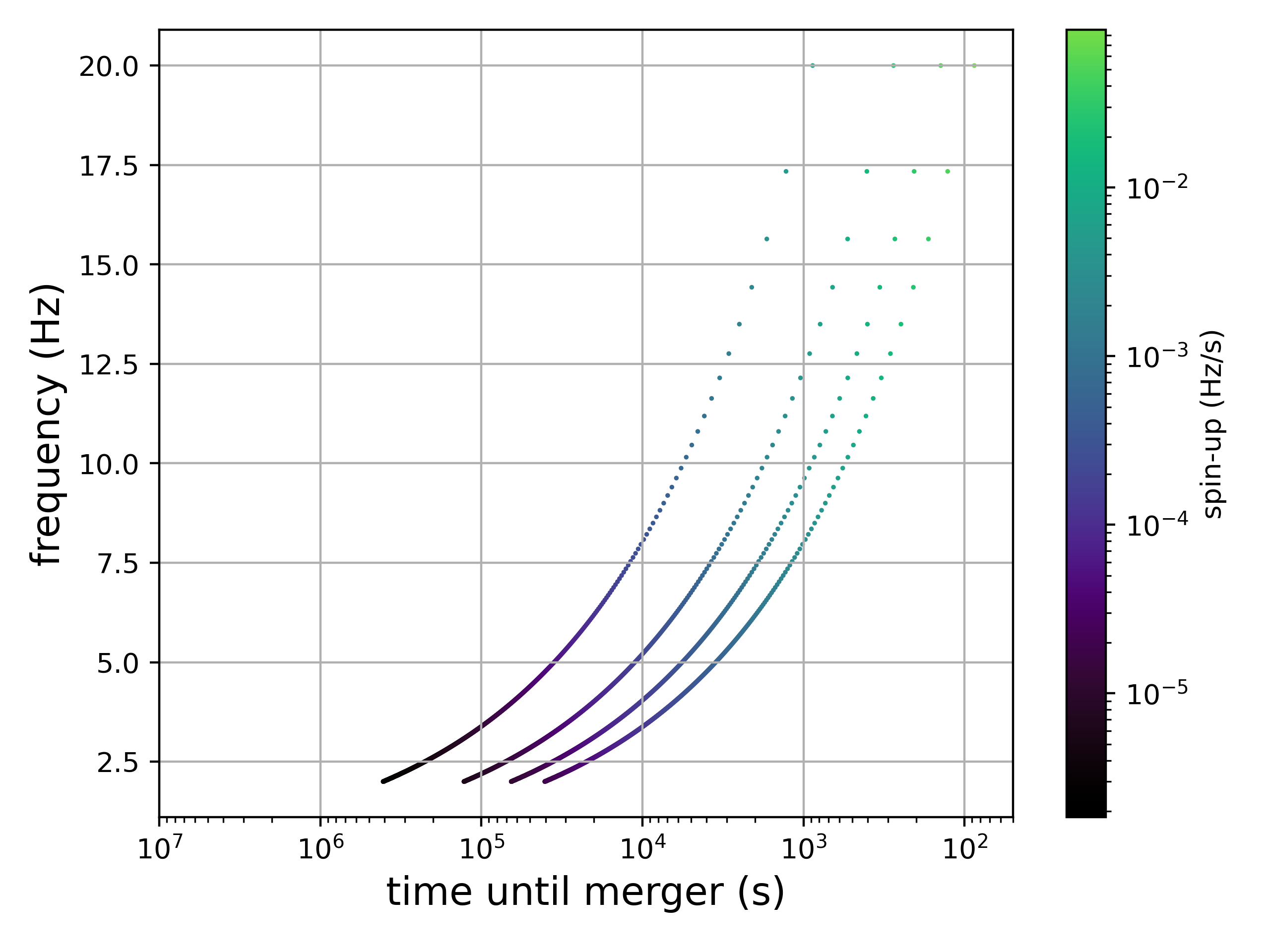
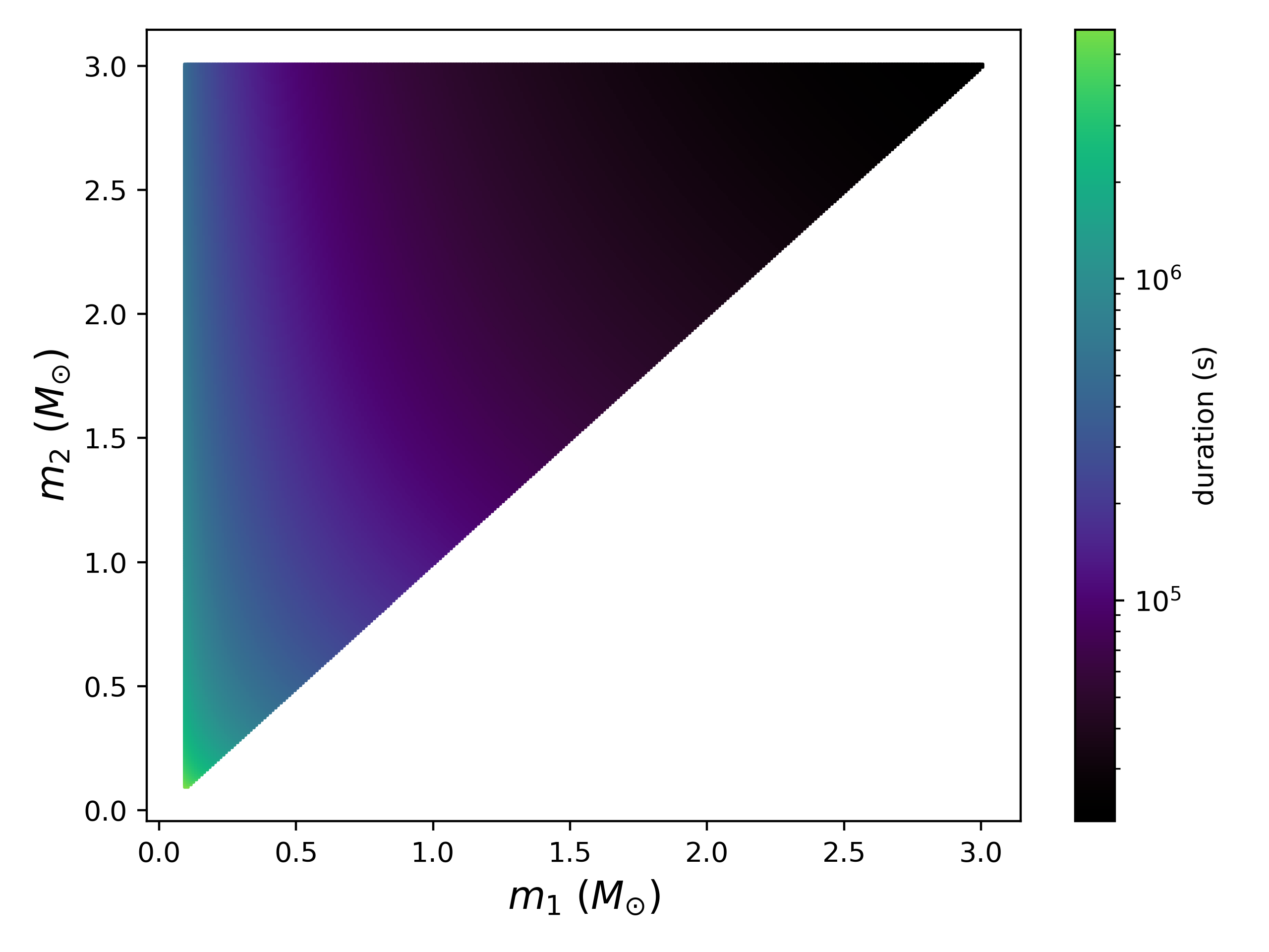
In addition to Fig. 1, we show, in Fig. 2, the time that a binary neutron-star binary would spend in the $2-20$ Hz band, as a function of the individual component masses $m_{1}$ and $m_{2}$. Coupled with Fig. 1, we see that signals with small $\dot{f}$ can last for a long time, making them similar to a continuous-wave signal. However, we will have to use a method that can handle not just quasi-monochromatic signals, but ones that follow a power law, as detailed in the next section.

Figure 2: $m_{1}/m_{2}$ space describing how long signals would last in the low-frequency ($2-20$ Hz) band.

III Search method: Generalized Frequency-Hough

We propose a method based on the Generalized Frequency-Hough, a “power-law track finder”, to search for inspiraling signals in Einstein Telescope and Cosmic Explorer. The Generalized Frequency-Hough transform is a pattern recognition technique that maps points in the time/frequency plane of the detector to lines in the frequency/chirp mass plane of the source, and was designed to search for signals that follow power-law frequency evolutions and that last $\mathcal{O}$(hours-days) Miller et al. (2018, 2021a). The method relies on making the following transformation of Eq. 3 to a new coordinate $x$:

$$x=f^{1-n}.$$ (6)

Once we have changed coordinates (by substituting Eq. 6 into Eq. 3), the signal’s frequency evolution becomes linear in the new space:

$$x=x_{0}+k(n-1)(t-t_{0}),$$ (7)

where we have also written $x_{0}=f_{0}^{1-n}$. Now, points in the time/$x$ plane are mapped to lines in the $x_{0}/k$ plane, and these two variables translate directly back to $f_{0}$ and $\mathcal{M}$.

In contrast to matched-filtering searches, we perform the Generalized Frequency-Hough analysis on a time/frequency “peakmap”, not a frequency series of Fourier transformed strain. We divide the strain $h(t)$ time-series into chunks of length $T_{\text{FFT}}$, fast Fourier transform each one (keeping the phase within each $T_{\text{FFT}}$), threshold the power in each frequency bin, and select local maxima above this threshold. The power in each time/frequency point that survives these two checks is called a “peak”, and, for the purposes of the Generalized Frequency-Hough, we label each peak simply with a “1”, and all other points 0. The Generalized Frequency-Hough, therefore, acts on a collection of 1s in the time/frequency plane - the value of the equalized power is not important.

While it should be better to sum raw power to obtain the highest possible sensitivity, the non-Gaussian, non-stationary nature of the noise allows strange artifacts to pop up throughout these chunks, which would effectively blind us to potential inspirals. This choice has been extensively studied in the context of continuous-wave Frequency-Hough searches Astone et al. (2005, 2014), and has been shown to be robust against noise disturbances. In particular, powerful noise lines that appear at or wander around a certain frequency, or glitches that occur throughout the run, are only given a weight of “1” in the peakmap, thus greatly reducing their effects on real gravitational-wave signals present in the data.

We choose $T_{\text{FFT}}$ on the basis of the spin-up, given in Eq. 1, by ensuring that the frequency modulation induced by $\dot{f}$ is confined to half a frequency bin, in each fast Fourier transform:

$$\dot{f}T_{\text{FFT}}\leq\frac{1}{2T_{\text{FFT}}}\rightarrow T_{\text{FFT}}\leq\frac{1}{\sqrt{2\dot{f}}}.$$ (8)

The analysis choices that we make to construct the peakmap fix the sensitivity of the search, i.e. the choices of fast Fourier Transform length $T_{\text{FFT}}$ and duration of the map $T_{\text{obs}}$. The sensitivity of the Generalized Frequency-Hough search towards inspiraling binary systems has already been computed in Miller et al. (2021b), and is rewritten here, in terms of the maximum (luminosity) distance reach at a particular confidence level:

$$d_{\rm max}=\frac{C}{4}\left(\frac{G\mathcal{M}}{c^{2}}\right)^{5/3}\left(\frac{\pi}{c}\right)^{2/3}\frac{T_{\text{FFT}}}{\sqrt{T_{\text{obs}}}}\left(\sum_{i}^{N}\frac{f^{4/3}_{i}}{S_{n}(f_{i})}\right)^{1/2}\\ \times\left(\frac{p_{0}(1-p_{0})}{Np^{2}_{1}}\right)^{-1/4}\sqrt{\frac{\theta_{\rm thr}}{\left(CR_{\rm thr}-\sqrt{2}\mathrm{erfc}^{-1}(2\Gamma)\right)}}.$$ (9)

Here, $C$ is a geometric factor arising from averaging over an L-shaped ($=4.02$) or triangle-shaped ($=4.64$) detector, $\theta_{\rm thr}$ is the threshold for peak selection selection in the equalized spectra when constructing the peakmap, $p_{0}=e^{-\theta_{\rm thr}}-$ $e^{-2\theta_{\rm thr}}$ $+\frac{1}{3}e^{-3\theta_{\rm thr}}$ is the probability of selecting a peak above the threshold $\theta_{\rm thr}$ if the data contains only noise, $p_{1}$ = $e^{-\theta_{\rm thr}}-$ 2$e^{-2\theta_{\rm thr}}$ $+e^{-3\theta_{\rm thr}}$ , $CR_{\rm thr}$ is the threshold on the critical ratio we use to select candidates in the Generalized Frequency-Hough map, $N=T_{\text{obs}}/T_{\text{FFT}}$, and $\Gamma$ is the chosen confidence level.

IV Sensitivity estimate

IV.1 Optimized sensitivity

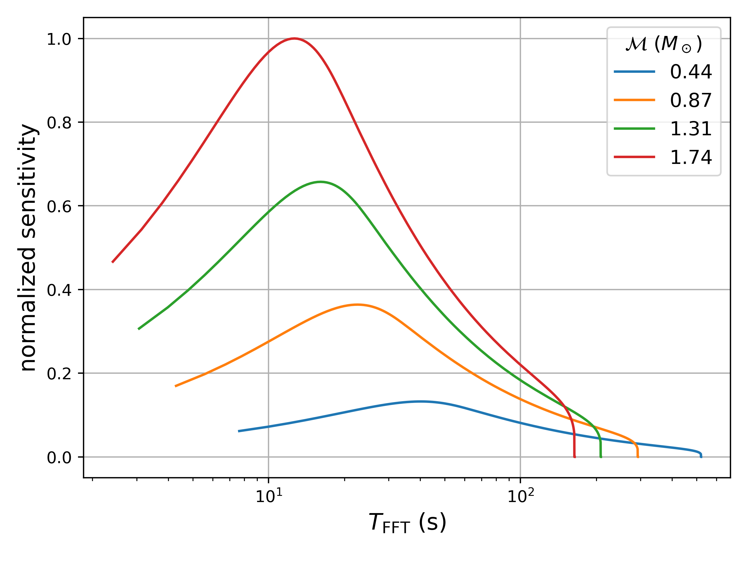
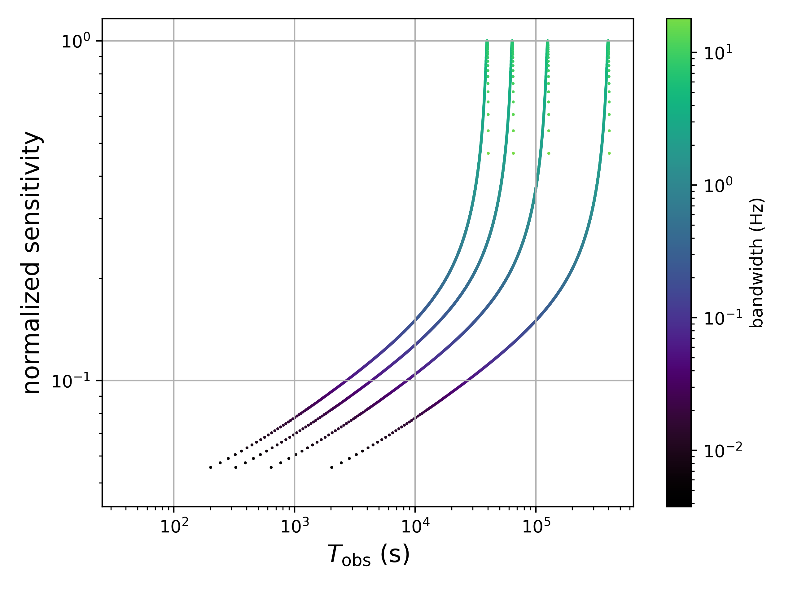
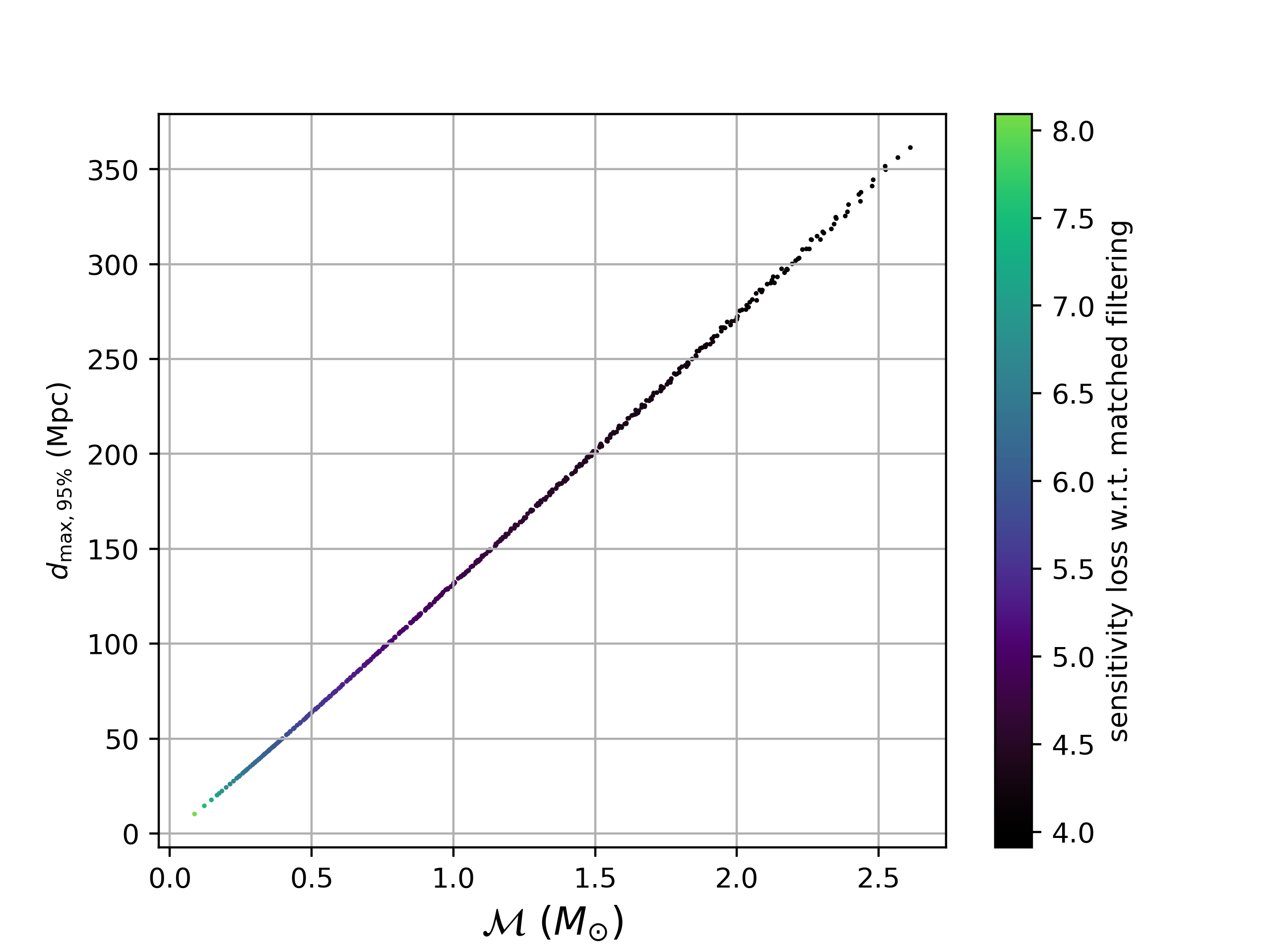
Binary neutron star inspirals will be observable for a fraction of the total duration of an observing run in Einstein Telescope. In matched filtering, observing the signal for as long as possible, thereby accumulating signal power across all frequency bins, results in the best sensitivity towards a particular source, assuming that one can generate a waveform for the duration of the signal. However, in semi-coherent approaches, the need to break the data into chunks of $T_{\text{FFT}}$, based on the spin-up of the binary system, implies that it may actually be optimal to not observe for the whole duration of the signal, but to cutoff the observation time at a fixed frequency. We currently do not vary $T_{\text{FFT}}$ as a function of the signal frequency, and typically pick $T_{\text{FFT}}$ based on the maximum $\dot{f}$ in a particular frequency band, which occurs at the highest frequency (Eq. 1). Therefore, if we observe for a shorter amount of time, i.e. not including the higher frequencies, $\dot{f}$ is smaller, meaning that $T_{\text{FFT}}$ can be longer. Thus, we consider the interplay between $T_{\text{obs}}$ and $T_{\text{FFT}}$ as a function of the signal parameters over which we search using Eq. 9. In Fig. 3(a), we show the optimal distance reach as a function of $T_{\text{FFT}}$ length, which corresponds to a particular $T_{\text{obs}}$ and bandwidth, shown in Fig. 3. The different curves refer to different chirp masses, as in Fig. 1. Essentially, it does not pay to observe for as long as possible within a $2-20$ Hz band with the longest possible $T_{\text{FFT}}$; instead, we should cut off the observation time before the signal reaches 20 Hz, which corresponds to a fixed bandwidth given by the value on the colorbar in Fig. 3.

(a)

Figure 3: Left: normalized sensitivity as a function of $T_{\text{FFT}}$ length, for different chirp-mass systems, when analyzing $2-20$ Hz, when varying $T_{\text{obs}}$ and $T_{\text{FFT}}$ in Eq. 9. The peak corresponds to the $T_{\text{FFT}}$ that maximizes our sensitivity to different compact binary coalescences. Right: Normalized sensitivity vs observation time, optimized by amount of frequency band analyzed and $T_{\text{FFT}}$, for a signal starting at 2 Hz. The chirp mass is indicated for each curve, and matches those in Fig. 1.

IV.2 Comparison to the matched filter

The matched filter can model exactly the inspiral portion of the binary neutron-star system. However, it comes at a very high computational cost.

We perform a quantitative comparison between the Generalized Frequency-Hough Transform and the matched filter. We borrow the formalism from Astone et al. (2014) and derive the minimum possible amplitude that could be detected via matched filtering.

The matched filter is defined as follows:

$$\lambda\equiv 4\int_{f_{\rm min}}^{f_{\rm max}}df\frac{|\tilde{h}(f)|^{2}}{S_{n}(f)},$$ (10)

where $|\tilde{h}(f)|^{2}$ is the Fourier Transform of the inspiraling binary system, given by Maggiore (2008)

$$|\tilde{h}(f)|^{2}=\frac{5}{6}\frac{4}{25}\frac{1}{4\pi^{4/3}}\frac{c^{2}}{d^{2}}\left(\frac{G\mathcal{M}}{c^{3}}\right)^{5/3}f^{-7/3}.$$ (11)

Analogously to the Frequency-Hough Astone et al. (2014), we would like to compute the minimum detectable amplitude (or maximal distance reach) at a given confidence level for a matched filtering search, accounting for the fact that we have real search limitations, e.g. the need to select a fixed number of candidates. This information is encoded in a threshold on $\lambda$: since we know the distribution of spectral power is exponential, the probability that a particular frequency bin contains power $S$ larger than some threshold $S_{\rm thr}$ is:

$$P(S>S_{\rm thr})=e^{-S_{\rm thr}}.$$ (12)

If we impose that the number of candidates above $S_{\rm thr}$ is $N_{\rm cand}$, then we have $N_{\rm tot}\cdot e^{-S_{\rm thr}}=N_{\rm cand}$, so:

$$S_{\rm thr}=-\log\left(\frac{N_{\rm cand}}{N_{\rm tot}}\right),$$ (13)

where $N_{\rm tot}$ is the total number of points in the source parameter space. This ratio is the false alarm probability of the search. If we fix $\frac{N_{\rm cand}}{N_{\rm tot}}=10^{-4}$, $S_{\rm thr}$=9.21. In practice, this ratio will be fixed based on the search that we actually perform, and the number of follow-ups that we can afford to do. In an all-sky search, this ratio is $\mathcal{O}(10^{-30})$ Astone et al. (2014), so our choice is quite conservative; however, we note that the sensitivity loss with respect to matched filtering does not differ by more than a factor of $\sim 2-3$ for even lower false alarm probabilities than what we choose.

The spectrum distribution in the presence of a signal of spectral amplitude $\lambda$ is a non-central $\chi^{2}$ with two degrees of freedom. The probability of having a spectrum value, in a given frequency bin, larger than a threshold $S_{\rm thr}$ is then

$$P(S>S_{\rm thr};\lambda)=\int_{S_{\rm thr}}^{\infty}dSe^{-S-\frac{\lambda}{2}}I_{0}\left(\sqrt{2S\lambda}\right),$$ (14)

where $I_{0}$ is the zeroth-order Bessel function of the first kind. Eq. 14 is the probability to detect a gravitational-wave signal; therefore, if we would like to compute the minimum spectral amplitude that is detectable $95\%$ of the time, we set $P(S>S_{\rm thr};\lambda)=0.95$ and compute $\lambda_{\rm min}$ such that we achieve this probability by numerically integrating Eq. 14. We find $\lambda_{\rm min}=34$ .

Now, combining equations 5 and 11, we can express $|\tilde{h}(f)|^{2}$ in terms of $h_{0}$:

$$|\tilde{h}(f)|^{2}=\frac{1}{30\pi^{8/3}}\frac{h_{0}^{2}}{16}\left(\frac{G\mathcal{M}}{c^{3}}\right)^{-5/3}f^{-11/3},$$ (15)

and then use Eq. 10 to write $h_{0}$ in terms of $\lambda_{\rm min}$:

$$h_{0,\rm min}^{\rm MF}=\sqrt{120\pi^{8/3}\lambda_{\rm min}\left(\frac{G\mathcal{M}}{c^{3}}\right)^{5/3}\left(\int_{f_{\rm min}}^{f_{\rm max}}df\frac{f^{-11/3}}{S_{n}(f)}\right)^{-1}}.$$ (16)

We can compare this expression to that computed for the semi-coherent Generalized Frequency-Hough search Miller et al. (2021b):

$$h_{0,\rm min}^{\rm GFH}=\frac{4.02}{N^{1/4}\theta_{\rm thr}^{1/2}}\sqrt{\frac{N}{T_{\text{FFT}}}}\left(\sum_{i}^{N}\frac{f_{i}^{4/3}}{S_{n}(f_{i})}\right)^{-1/2}f_{0}^{2/3}\\ \times\left(\frac{p_{0}(1-p_{0})}{p^{2}_{1}}\right)^{1/4}\sqrt{\left(CR_{\rm thr}-\sqrt{2}\mathrm{erfc}^{-1}(2\Gamma)\right)},$$ (17)

and compute the ratio

$$R\equiv\frac{h_{0,\rm min}^{\rm GFH}}{h_{0,\rm min}^{\rm MF}},$$ (18)

in order to gauge how much worse our semi-coherent method will be, as a function of chirp mass. We show this ratio in Fig. 4. We note that smaller chirp mass systems can be observed for longer times, but, as in Astone et al. (2014), this actually implies a greater sensitivity loss for our method compared to matched filtering. However,, the “area of interest” for binary neutron star inspirals is at least $\mathcal{O}(M_{\odot})$, and here, the sensitivity loss is around $\sim 4$, and would be lower depending on our choice of false alarm probability, and the number of candidates that we could afford to follow up in a real search.

Figure 4: Luminosity distance reach and sensitivity loss with respect to matched filtering colored as a function of chirp mass. Observing for longer periods of time (corresponding to smaller chirp masses) increases the sensitivity loss compared to larger chirp masses, since matched filtering can accumulate more signal power over time compared to the semi-coherent Generalized Frequency-Hough, due to reducing the $T_{\text{FFT}}$ length (see Fig. 3(a)). Valid for signals that span $2-20$ Hz.

IV.3 Data gaps, non-stationary noise and overlapping signals

The Generalized Frequency-Hough sums the presence of a peak in the time/frequency peakmap. Therefore, we inherently work with data that are not continuous in the time and frequency domains, meaning that gaps, for any period of time, do not pose a systemic problem to our method. Furthermore, the detector power spectral density is estimated quickly in each FFT we take using an auto-regressive method Astone et al. (2005), meaning that changing, non-stationary noise, or different noise properties at one end of a gap and the other, do not affect our method’s ability to work.

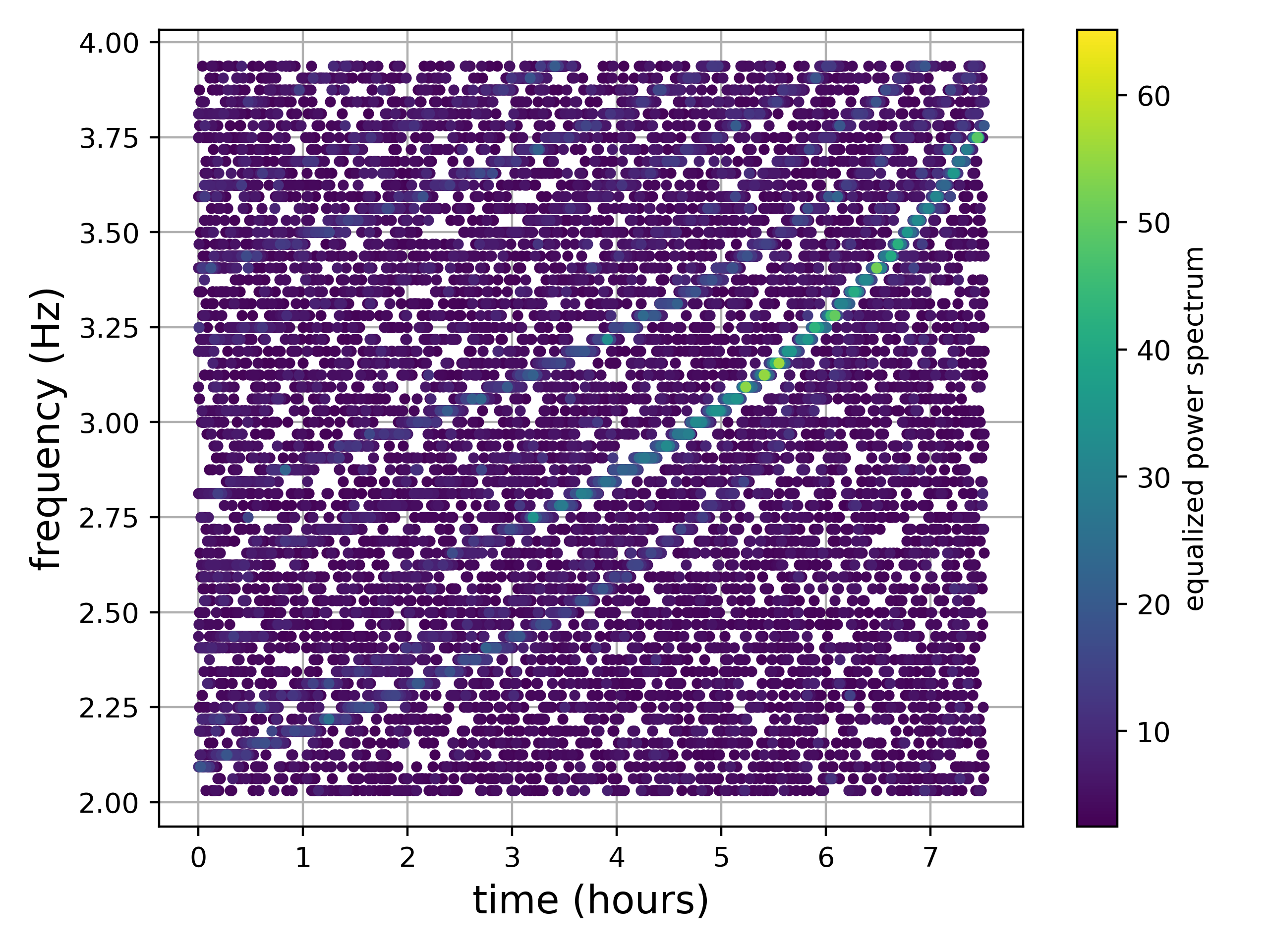
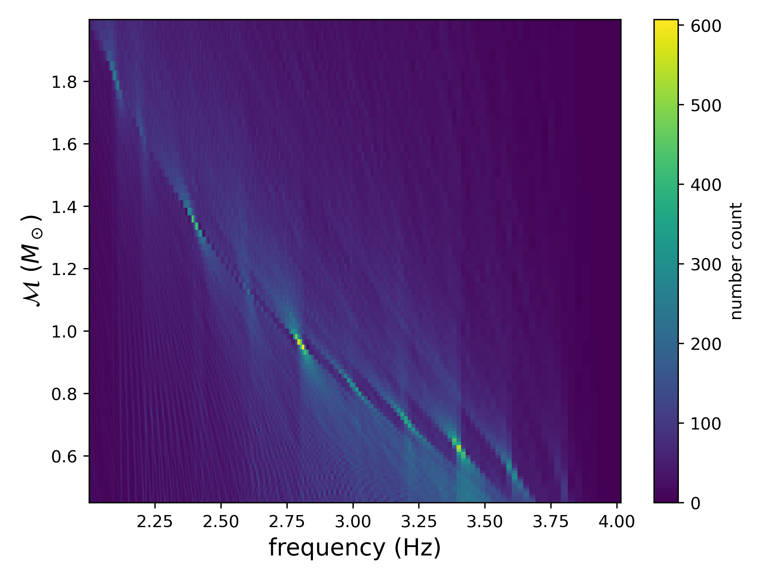
We illustrate these concepts in Fig. 5(a), in which we plot a time/frequency peakmap with ten signals that exist over the same time and frequency ranges in the left-hand panel (the white spaces are gaps due to thresholding this map). The Generalized Frequency-Hough maps points in the peakmap to lines in the frequency/chirp mass plane of the source, and we can see here that each of the ten signals is well localized in a different pixel in Fig. 5. This occurs because each system has a different frequency at the start of the observation, and a different chirp mass. Of course, we could have also considered signals that have the same start frequency with different chirp masses, or the same chirp mass with different starting frequencies. However, the signals would still be localized into different pixels in Fig. 5. The power of the Generalized Frequency-Hough is that it sums time/frequency peaks along certain independent tracks, ensuring that signal parameters are well localized in the frequency/chirp mass plane.

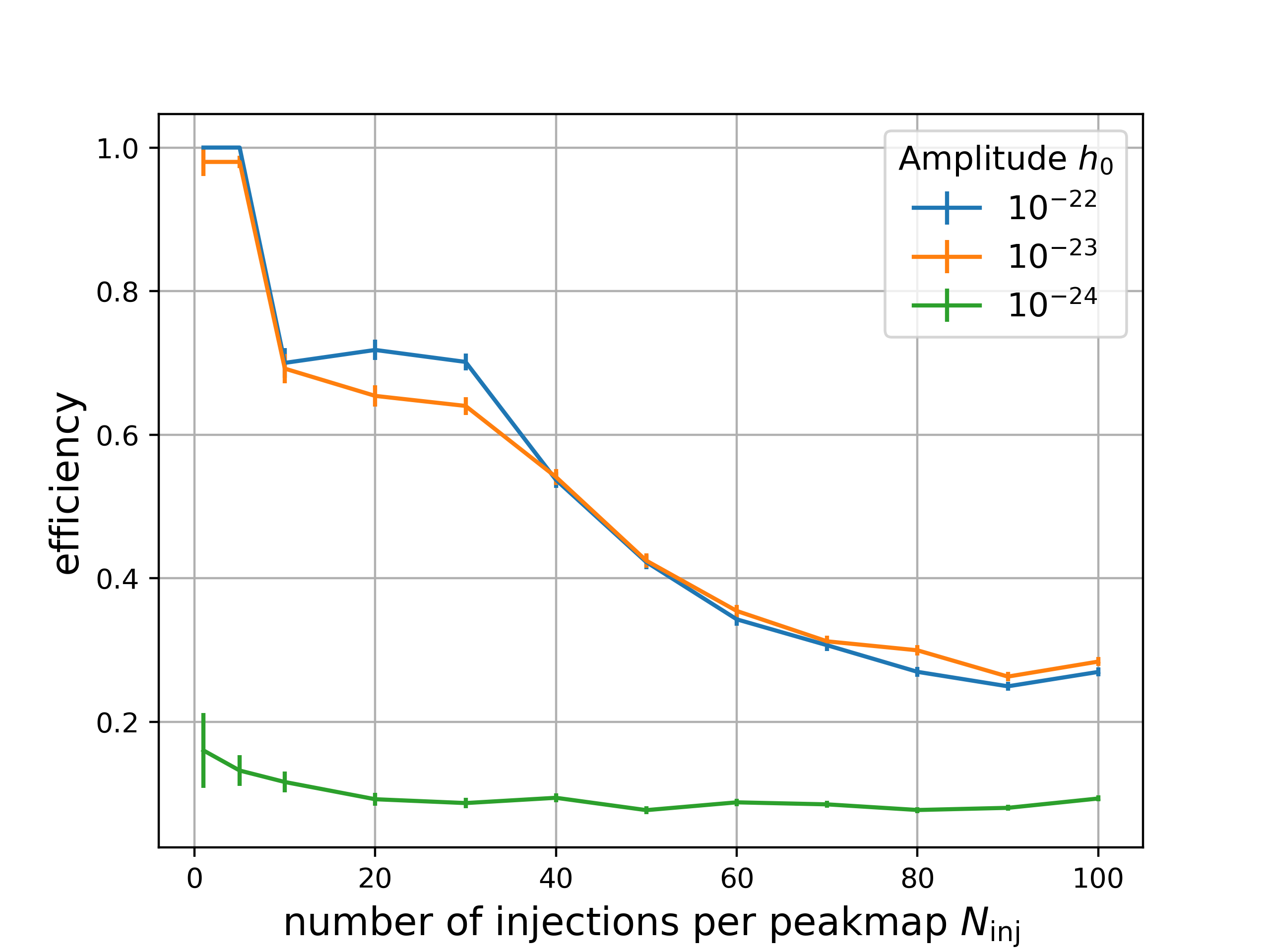
We have also studied the impact of a large number of signals present in the data on the performance of the Generalized Frequency-Hough. In Fig. 6, we plot the fraction of detectable signals as a function of the number of injections present in the peakmap $N_{\rm inj}$, marginalizing over starting frequencies uniformally distributed between [4.01,6.97] Hz, chirp masses ([0.33,1.14]$M_{\odot}$), and signal durations ([200,10000] seconds). For each $N_{\rm inj}$, we performed 50 simulations, for three different signal amplitudes. We can see that while a small number, $\sim 5$, of simultaneously present number of injections does not impact the efficiency, also shown in lia , the efficiency degrades between $10-100$ injections. We note that this efficiency could be improved via a better estimation of the auto-regressive spectrum used to construct the peakmaps Pierini et al. (2022), which has been optimized for singular, weak monochromatic signals. Moreover, our efficiency represents the realistic case in which we do not know which signals will be present in any given peakmap – of course, if we only considered a couple of signals present simultaneously, and also constructed the peakmap with the appropriate $T_{\text{FFT}}$ to be optimally sensitive to each signal, these efficiencies would improve. However, when the detector turns on, we will not know which signals are present, so we cannot tune $T_{\text{FFT}}$ and the size of the peakmap for each signal. Therefore, our results represent a realistic test-case of unknown overlapping signals.

(a)

Figure 5: Ten signals have been injected in white noise between 2-4 Hz, and are recovered by the Hough transform. Signals overlapping in time and in frequency can be easily isolated in the Hough plane. $\sqrt{S_{n}}\sim 8\times 10^{-24}\text{ Hz}^{-1/2}$. The amplitude for all signals is the same at $t=0$ ($h_{0}=10^{-23}$), but over time, each changes in different ways based on the frequency evolution and the chirp mass of the injected signal. In the case of non-Gaussian, non-stationary noise, this method has been tested extensively in Miller et al. (2018); Abbott et al. (2019).

Figure 6: Efficiency as a function of number of injected signals per peakmap, where 50 simulations at each $N_{\rm inj}$ were performed. Even for strong signals, efficiency degrades rapidly past $N_{\rm inj}\sim 30$. “Efficiency” is defined as the fraction of the total number of signals injected across all simulations that are recovered by the Generalized Frequency-Hough.

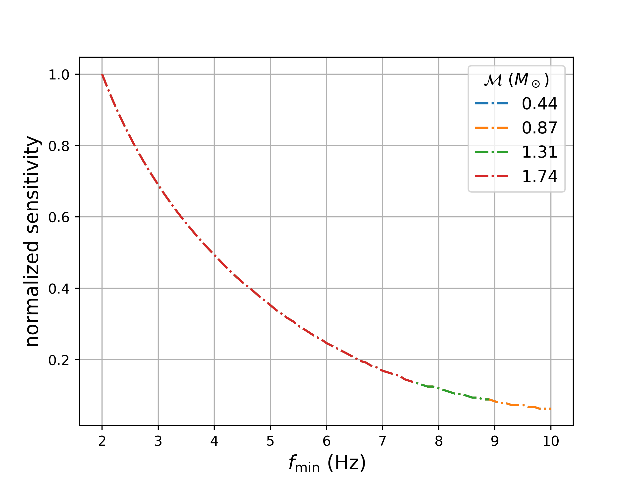
IV.4 Sensitivity robustness against different $f_{\text{min}}$

Throughout this paper, we have consistently chosen the minimum frequency at which we compute sensitivity estimates to be $f_{\text{min}}=2$ Hz. However, the true frequency floor will vary depending on the nature of the noise in Einstein Telescope, and it is not clear yet whether such amazing sensitivity at 2 Hz will be achievable Beker et al. (2015); Badaracco et al. (2020). We therefore consider how our results will change with respect to differing $f_{\text{min}}$. We vary the beginning frequency $f_{\text{min}}$ and compute the sensitivity, noting that a higher $f_{\text{min}}$ implies shorter observation time and less accumulated power, as shown in Fig. 7. Our sensitivity appears to vary by by no more than a factor of 10 across the chosen $\mathcal{M}$ with respect to the $f_{\text{min}}=2$ Hz case. We note that in Fig. 7, the curves for each chirp mass do not all extend to 10 Hz because we set a threshold of at least 10 minutes to observe, and higher chirp mass systems will not last for longer than that between $f_{\text{min}}$ and 20 Hz.

Figure 7: Normalized sensitivity as a function of the beginning analysis frequency. At $f_{\text{min}}=5$ Hz, we see that we would only be 35% as sensitive to inspiraling systems compared to if we observed them starting from $f_{\text{min}}=2$ Hz.

V Enabling multi-messenger astronomy

V.1 Sky localization

Part of the need for early warning is to provide astronomers not only with intrinsic source parameters but also sky position. In our method, depending on the chirp mass of the system, the frequencies at which we observe it, and the $T_{\text{FFT}}$ with which we analyze the data, the accuracy of sky localization will be different.

Figure 8: Finest possible sky localization based on a single-interferometer analysis as a function of chirp mass, assuming that the signal frequency evolution can be completely demodulated after estimating the chirp mass and initial frequency of the system, resulting in a purely monochromatic signal. For an equal-mass system of $1.4M_{\odot}$ ($\mathcal{M}=1.22M_{\odot}$), this plot is consistent with the estimations present in Nitz and Dal Canton (2021) for a single Einstein Telescope interferometer, though we consider only the $2-20$ Hz band.

The Generalized Frequency-Hough will provide an estimation of orbital frequency and chirp mass. In an initial search, for high chirp masses $\mathcal{O}(1M_{\odot})$, $T_{\text{FFT}}$ and the gravitational-wave frequency are too small to construct a sky grid (that is to say, we cannot perform sky localization in the first pass of this method). This is because because the Doppler shift is directly proportional to the frequency, and since $T_{\text{FFT}}$ is quite small compared to its values continuous-wave all-sky searches, the Doppler shift is contained within one (large) frequency bin, since the increase in gravitational-wave frequency due to the inspiral is greater than the frequency shift induced by the Doppler motion. However, after we estimate gravitational-wave frequency and chirp mass, we can correct for the phase evolution of the signal, neglecting higher-order post-Newtonian corrections. If a perfect correction is made, the signal would become monochromatic; thus, we would be able to set $T_{\text{FFT}}\sim T_{\text{obs}}$. In practice, we cannot make a perfect correction given the coarseness in the chirp mass and gravitational-wave frequency grids, but we can understand how our resolution in the sky will improve with each pass of our method. As in standard all-sky searches, we would perform a hierarchical follow-up, in which we will increase $T_{\text{FFT}}$ gradually, usually by a factor of 2 in each pass Abbott et al. (2022e). As we constrain more and more the signal parameters, we will also obtain a finer and finer resolution in the sky, but of course, the time that will remain to warn astronomers will decrease.

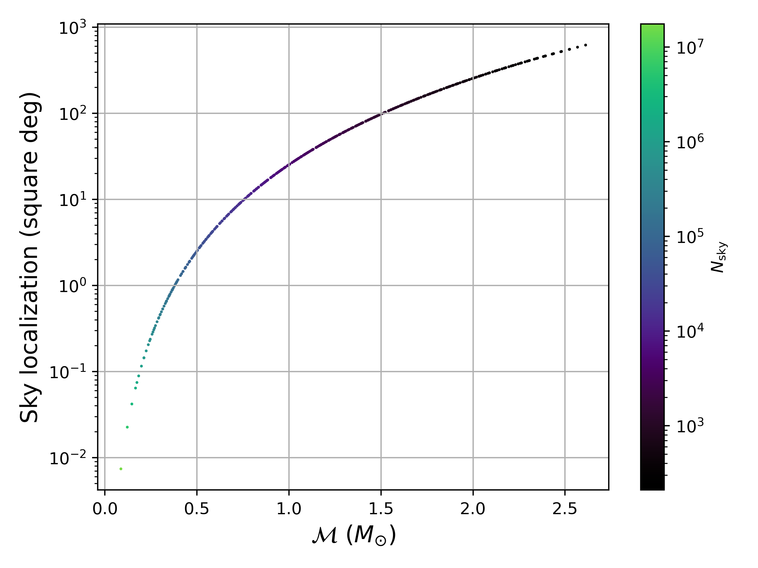
Assuming that we can make a perfect correction and use $T_{\text{FFT}}=T_{\text{obs}}$, in Fig. 8, we plot the finest possible sky resolution, in square degrees, and the number of sky points in the grid, as a function of chirp mass, using a single interferometer (one interferometer of a triangular Einstein Telescope instrument). This figure is generated by following the formalism in Astone et al. (2014), Eq. 35$-$43, which accounts for the Doppler modulation when constructing a grid on the sky to perform a continuous-wave analysis. We can see that the sky localization for higher chirp mass systems is worse than that for weaker ones. This is due to the fact that the higher chirp mass systems have larger spin-ups, and thus have smaller durations. In order to achieve this localization, in practice we will need to progressively increase $T_{\text{FFT}}$ after recovering $f_{0}$ and $\mathcal{M}$, and allow for the uncertainties in each parameter.

(a)

Figure 9: Left: Maximum time available to warn astronomers that a merger of two compact objects will occur at different distances. Right: fraction of coalescence time necessary to observe a signal at a particular chirp mass is colored. At higher distances (and lower masses), more time is needed to obtain a given distance reach. If the source is closer, then we do not have to observe for as long as if the source were farther, at a fixed chirp mass.

V.2 Early warning

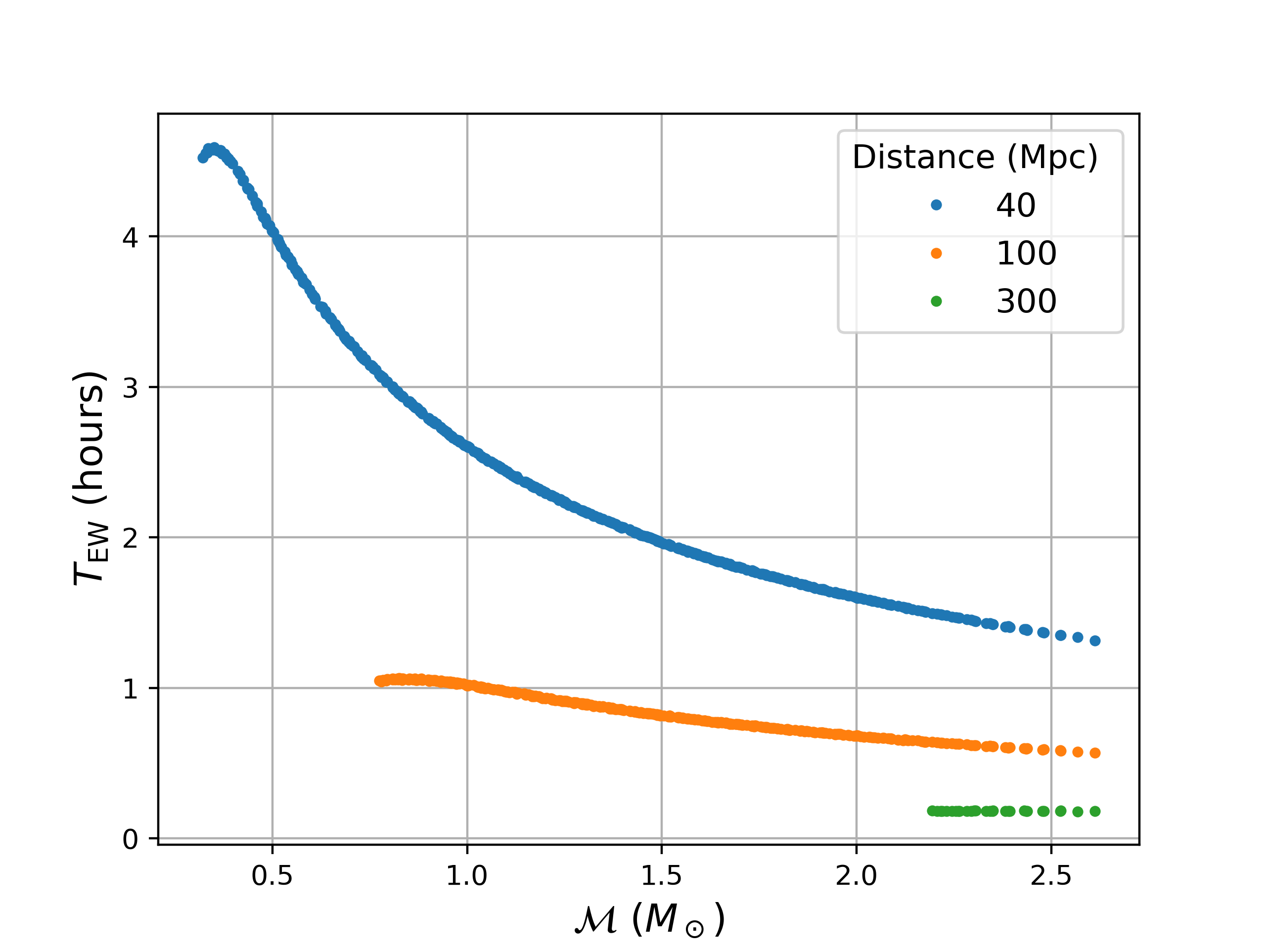
The next generation of gravitational-wave detectors will be sensitive at low-enough frequency such that, in principle, ample time will exist to warn astronomers that a merger of two compact objects will happen somewhere in the sky. We define the maximum time that we will have to warn astronomers, $T_{\text{EW}}$, as:

$$T_{\text{EW}}\equiv t_{\text{coal}}-T_{\text{obs}},$$ (19)

where $T_{\text{obs}}$ is the time that we observe the inspiral such that we obtain the maximum distance reach, as indicated in Fig. 3, and $t_{\text{coal}}$ is the time to coalescence, calculated at $f_{\text{min}}=2$ Hz, the starting frequency of the band analyzed.

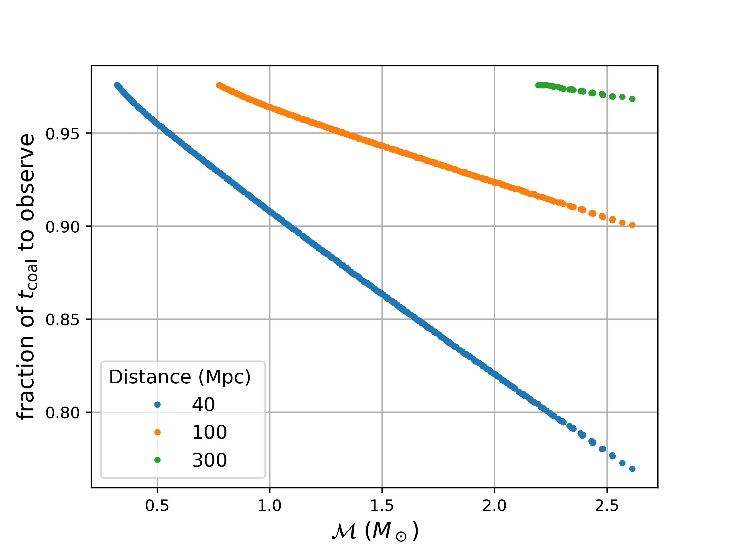
In Fig. 9(a), we plot $T_{\text{EW}}$ as a function of $\mathcal{M}$ if, at that particular $\mathcal{M}$, we could detect an inspiraling system at least 40, 100 or 300 Mpc away. For the 40 Mpc curve, $T_{\text{EW}}$ time peaks at a chirp mass of $\sim 0.25M_{\odot}$, then steadily falls off. The peak occurs because of the interplay between the accumulation of signal-to-noise ratio over time, and the duration of the signal. At higher chirp masses, the signals are shorter, and a smaller fraction of $t_{\text{coal}}$ is necessary to reach the chosen distance.

For the 100 Mpc curve in Fig. 9(a), systems below 1$M_{\odot}$ cannot be reached at 100 Mpc. In this case, we are observing a little bit less and less as we increase the chirp mass, but we still need to observe for a large fraction of $t_{\text{coal}}$ (Fig. 9), $\mathcal{O}(10^{4})$ seconds for all $\mathcal{M}>1M_{\odot}$. We note that, as expected, $T_{\text{EW}}$ is smaller for larger distances, since we need to observe for a larger fraction of $t_{\text{coal}}$ to reach a larger distance.

VI Projected merger rates and constraints

As with any method to search for inspiraling systems in next-generation detectors, we can provide estimates of how well we can constrain various astrophysical quantities in the future, including the merger rates of compact objects, as well as dark-matter properties. We describe how we will obtain these constraints in the following two subsections.

VI.1 Neutron-star merger rate densities

In order to compute merger rate densities for these systems, we adopt the formalism present in Biswas et al. (2009), recalling the following equation:

$$\mathcal{R}_{95\%,i}=\frac{3.00}{\left\langle VT\right\rangle_{i}},$$ (20)

where $\mathcal{R}_{95\%,i}$ is the merger rate density at a given chirp mass $i$, and $\left\langle VT\right\rangle_{i}$ is the average space-time volume enclosed for a given chirp mass, given by Abbott et al. (2016a, b); Singh et al. (2022, 2023):

$$\left\langle VT\right\rangle_{i}=T\int\mathrm{d}z\,\mathrm{d}\theta\,\dfrac{\mathrm{d}{V_{c}}}{\mathrm{d}{z}}\frac{1}{1+z}s_{i}(\theta)f(z,\theta),$$ (21)

where $f(z,\theta)=\Gamma$ in Eq. 9 and, in this case, is calculated from inputting a variety of possible source luminosity distances, and $\theta=\mathcal{M}$. $\dfrac{\mathrm{d}{V_{c}}}{\mathrm{d}{z}}$ is the differential co-moving volume as a function of redshift, whose values depend only on cosmology, and is given in App. A.

We make the assumption as in Kim et al. (2003): that the population follows the observed sources:

$$s_{i}(\theta)=\delta\left(\theta-\theta_{i}\right),$$ (22)

where $\delta$ is the Dirac delta function and $\theta_{i}$ are the parameters of source type $i$.

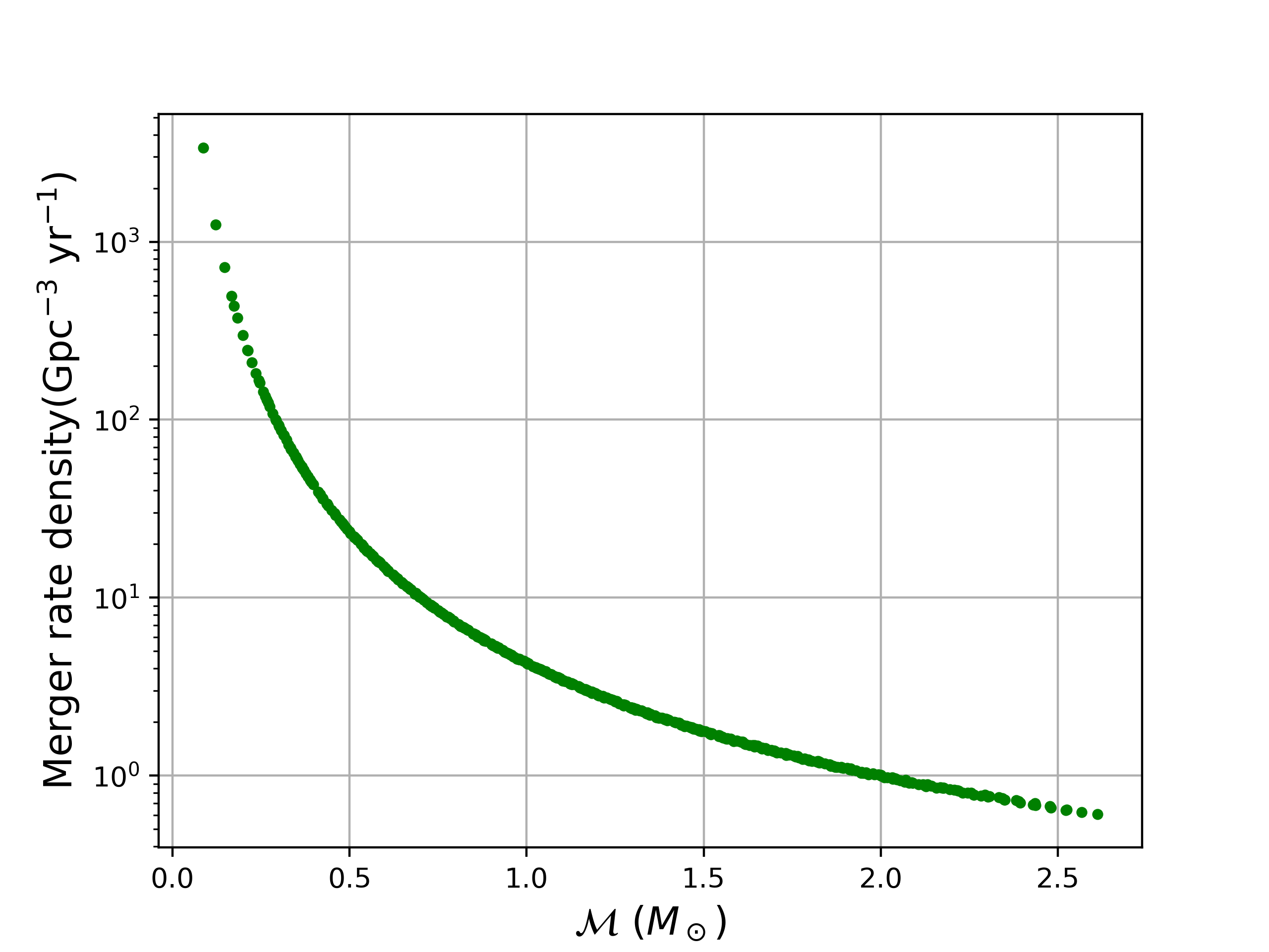
From these equations and the distance reaches computed in earlier sections, we can arrive at merger rate density estimates for compact binary systems with different chirp masses, given in Fig. 10. These projected constraints can be used to exclude binary population evolution models as to provide crucial information about the evolutionary scenarios. We test these constraints against some of the binary evolution models for population I and II field BNSs, whose details are given in App. B. We find that after $\sim 13$ years of observation, these models would begin to be excluded with our method.

Figure 10: Projected merger rate densities, treating each chirp mass as a separate population of compact objects.

VI.2 Primordial black hole binaries

While we have called the inspiraling compact objects in this paper “neutron stars”, we could have easily named them “primordial black holes”, especially those with sub-solar masses Carr et al. (2019); Green and Kavanagh (2021). In fact, the Generalized Frequency-Hough only considers two objects with a certain chirp mass, and makes no assumptions about what these objects actually are.

By using cosmological rate predictions for early primordial black hole binaries and of primordial black hole binaries in clusters, the rate densities in Fig. 10 can be translated into projected constraints on the dark matter fraction of primordial black holes. We use the analytical prescriptions from Raidal et al. (2019); Hütsi et al. (2021) for the cosmological merger rates that assume a purely Poissonian primordial black hole spatial separation at formation, given by:

$$\mathcal{R}_{95\%,i}= 1.04\times 10^{-6}\,\mathrm{kpc}^{-3}\mathrm{yr}^{-1}f_{\rm sup}f(m_{\rm PBH})^{2}$$ (23)

$$\left(\frac{m_{\mathrm{PBH}}}{M_{\odot}}\right)^{-32/37}\left(f_{\rm PBH}\right)^{53/37},$$

which correspond to the rate per unit of logarithmic mass of the two binary black hole components $m_{\rm PBH}$. $f_{\rm PBH}$ is the dark matter density fraction made of primordial black holes and $f(m)$ is the density distribution of primordial black holes normalized to one ($\int f(m){\rm d}\ln m=1$). We have included a suppression factor $f_{\rm sup}$ that effectively takes into account a rate suppression due to the gravitational influence of early forming primordial black hole clusters, nearby primordial black holes and matter inhomogeneities Raidal et al. (2019).

For unequal-mass mergers, we consider the merging rate in the limit $m_{1}\gg m_{2}$:

$$\mathcal{R}_{95\%,i}= 5.28\times 10^{-7}\,\mathrm{kpc}^{-3}\mathrm{yr}^{-1}f_{\rm sup}f(m_{1})f(m_{2})$$ (24)

$$\left(\frac{m_{1}}{M_{\odot}}\right)^{-32/37}\left(\frac{m_{2}}{m_{1}}\right)^{-34/37}\left(f_{\rm PBH}\right)^{53/37}~{}.$$

and place constraints on an effective, model-independent parameter $\tilde{f}$, due to the heavy model-dependence of $f_{\rm sup}$:

$$\tilde{f}^{53/37}\equiv f_{\rm sup}f(m_{1})f(m_{2})f_{\rm PBH}^{53/37}$$ (25)

We choose to constrain $\tilde{f}$ because of the uncertainty in the value of $f_{\rm sup}$. For equal-mass primordial black holes and $f_{\rm PBH}=1$, one may expect $f_{\rm sup}\approx 2\times 10^{-3}$ Hütsi et al. (2021); Clesse and Garcia-Bellido (2022); Raidal et al. (2019), but the exact value of $f_{\rm sup}$ for wide mass functions and binaries with high mass ratios is largely uncertain and model dependent. For example, external tidal fields and highly eccentric orbits of low-mass PBHs may affect this parameter Eroshenko (2018); Cholis et al. (2016).

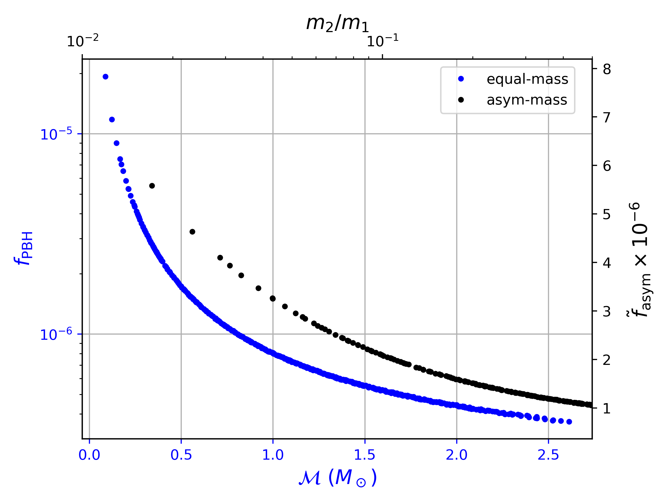
In Fig. 11, we plot the projected constraints on equal-mass and asymmetric-mass ratio binaries using the merger rates inferred in Fig. 10. For equal-mass systems (blue curve, blue text), in order to obtain a constraint on $f_{\text{PBH}}$, we assume $f_{\text{sup}}=2\times 10^{-3}$ and a monochromatic mass function, while for asymmetric mass-ratio binaries (black curve, black text), we constrain the effective parameter $\tilde{f}_{\rm asymm}$ for $m_{1}=2.5M_{\odot}$, motivated by the QCD phase transition Byrnes et al. (2018), and by observations of stellar-mass black holes.

Figure 11: Projected constraints on sub-solar and solar-mass PBH binaries, for both equal-mass and asymmetric mass ratio binaries, in terms of $f_{\text{PBH}}$ (blue) and $\tilde{f}$ (black). Blue and black axes correspond to the blue and black curve, respectively. $f_{\text{sup}}=2\times 10^{-3}$, and $m_{1}=2.5M_{\odot}.$

VII Conclusions

We have shown that the Generalized Frequency-Hough, and in general continuous-wave methods, can be adapted to search for long-lived compact binary inspirals in next-generation gravitational-wave detectors. The sensitivity, considering only quasi-Newtonian orbits, has been evaluated and compared to matched filtering, and was shown to be about a factor of $\sim 4$ worse for binary neutron star masses of $\mathcal{O}(M_{\odot})$. We have also quantified the maximum time available to warn astronomers of an incoming merger of two compact objects as a function of chirp mass and distance from us, ranging from a few hours to 10 minutes, and have shown that binary neutron stars with chirp masses greater than a solar mass could be detected at least 100 Mpc away from us. The sky localization, assuming that the signal’s frequency evolution can be completely demodulated, was also computed, and for binary neutron-star systems, could be as good as 1 square degree on the sky using a single interferometer. Additionally, we have provided preliminary results detailing the robustness of our algorithm against gaps, non-stationary noise, and overlapping signals, and have quantified the optimal way to perform a semi-coherent search by carefully picking $T_{\text{FFT}}$ and $T_{\text{obs}}$.

Our results are promising, and motivate further study of the Generalized Frequency-Hough and continuous-wave methods to tackle searches for compact binaries in next-generation gravitational-wave detectors. In the case of overlapping signals, we need to quantify the impact of multiple signals on the auto-regressive power spectral density estimation, as done in Pierini et al. (2022), revisit the choice of thresholds when constructing the time/frequency peakmap via simulations and statistical properties of the foreground/background, and determine how exactly to select candidates in the Hough plane in the presence of so many astrophysical signals. Furthermore, we must study the propagation of errors on parameters in the follow-up stages of the analysis, which will affect our ability to provide accurate sky localization to astronomers. We could also experiment with observing only the inspiral between, say, $2-3$ Hz, which would permit longer $T_{\text{FFT}}$, potentially allowing for more precise sky localization at the cost of some sensitivity, and finding ways to combine our sky position estimates with triangulation if the signal is seen in multiple detectors.

We must also consider the fact that the frequency evolution of the orbit may be affected by higher-order post-Newtonian terms Cutler and Flanagan (1994); Blanchet et al. (1995); Poisson and Will (1995); Baird et al. (2013), for which extensive waveform development has already been undertaken Pratten et al. (2021); Ossokine et al. (2020); Thompson et al. (2020); Matas et al. (2020). In order to obtain parameter estimations of each of these, i.e. the symmetric mass ratio, we can envision performing hierarchical Generalized Frequency-Hough transforms. First, we obtain estimates for $f_{0}$ and $M_{c}$, demodulate the signal, and then perform successive Generalized Frequency-Hough transforms on the remaining power-law terms in the post-Newtonian expansions. It is unclear what the computational cost of this will be, and whether this is necessary, since we could hand over our estimations of source parameters to a more sensitive matched filtering pipeline at this stage. Regardless, at least an implementation of the Generalized Frequency-Hough in low-latency will be necessary to perform real-time sky localization and parameter estimation of gravitational-wave signals from inspiraling compact binaries, and a proper comparison with matched filtering analyses in the presence of noise disturbances and overlapping signals will also be required.

Appendix A Computing $\left\langle VT\right\rangle_{i}$

We provide here a quick summary of the equations we use to compute the average space-time volume in Eq. 21. More details can be found in Abbott et al. (2016a); Taylor and Gair (2012).

The co-moving volume is:

$$\frac{dV_{c}}{dz}=4\pi D_{H}\frac{D_{L}(z)^{2}}{(1+z)^{2}E(z)}.$$ (26)

where $D_{L}$ is the luminosity distance, $D_{H}=c/H_{0}$, $H_{0}=70.4$ kms^-1Mpc^-1 is Hubble’s constant, $z$ is the redshift, and:

$$E(z)=\sqrt{{\Omega}_{m,0}(1+z)^{3}+{\Omega}_{k,0}(1+z)^{2}+{\Omega}_{\Lambda}(z)}.$$ (27)

Here, the parameters for the $\Lambda$ cold dark-matter ($\Lambda$CDM) model are: $\Omega_{m,0}=0.2726$, $\Omega_{k,0}=-0.0006$, where Jarosik et al. (2011):

$$\Omega_{\Lambda}(z)=\Omega_{\Lambda,0}\times{(1+z)}^{3(1+w_{0}+w_{a})}\times e^{-3w_{a}\left(\frac{z}{1+z}\right)}.$$ (28)

Here, $w_{0}=-1$ and $w_{a}=0$ are dark-energy (linear) equation of state parameters. For different global geometries of the Universe, $D_{L}$, is given by:

$$D_{L}(z|\mathcal{C})=(1+z)\times\mathcal{F}(z|\mathcal{C}),$$

$$\mathcal{F}(z|\mathcal{C})=\begin{cases}\frac{D_{H}}{\sqrt{\Omega_{k,0}}}\sinh\left(\sqrt{\Omega_{k,0}}\frac{D_{c}(z|\mathcal{C})}{D_{H}}\right),&\Omega_{k,0}>0,\\ D_{c}(z|\mathcal{C}),&\Omega_{k,0}=0,\\ \frac{D_{H}}{\sqrt{|\Omega_{k,0}|}}\sin\left(\sqrt{|\Omega_{k,0}|}\frac{D_{c}(z|\mathcal{C})}{D_{H}}\right),&\Omega_{k,0}<0,\end{cases}$$ (29)

The co-moving radial distance, $D_{c}(z)$, is given by

$$D_{c}(z)=D_{H}\int_{0}^{z}\frac{dz^{\prime}}{E(z^{\prime})},$$ (30)

Appendix B Constraining binary evolution models

Belczynski et al. (2020) generated a vast set of models of population I and II field binaries. The authors present a range of models and their rate densities. The rate density in each case is the result of several assumptions such as the cosmic star formation, metallicity evolution, the initial binary parameters and the implied delay time (between the birth of a binary and the final merger of two compact objects) distribution. The details of these models are summarised in Table 2 in Belczynski et al. (2020). The data for all these models is available on the StarTrack site. We calculate the detector frame merger rate density with our algorithm which gives the upper limit on the merger rate density in detector frame for a range of chirp masses up to redshift of $z\sim 0.08$, which we denote as $\mathcal{R}_{\rm pred}$. We compare the detector frame merger rate densities for BNSs as predicted by the nine models which were not excluded by the LVK merger rate predictions (see Figs. 24 and 25 in Belczynski et al. (2020)). We list the details in Table 1 below. We do not exclude any of these models given the constraints we estimate of the chirp masses, considering an observation time of 1 year. It would be possible to begin to exclude some of these models if we could observe for $\sim 15$ years.

model	min $\mathcal{M}$ $(M_{\odot})$	max $\mathcal{M}$ $(M_{\odot})$	$\mathcal{R}_{\rm pred}$ (Gpc-3 yr -1)	$\mathcal{R}_{95\%}$ (Gpc-3 yr -1)	Time to exclude (yr)
m13A	0.95	1.72	19.89	469.66	23.61
m23A	0.93	1.70	21.07	493.95	23.44
m30B	0.96	1.66	17.08	432.18	25.30
m33A	0.96	1.70	33.19	443.36	13.36
m40B	0.96	1.67	17.01	438.23	25.76
m43A	0.96	1.70	33.84	447.99	13.24
m50B	0.96	1.66	13.09	441.49	33.73
m60B	0.96	1.66	16.52	430.75	26.07
m70B	0.96	1.67	16.69	433.60	25.98

Table 1: The BNS merger rate densities predicted for different evolutionary models Belczynski et al. (2020).

References

- Abbott et al. (2021a) R. Abbott et al. (LIGO Scientific Collaboration, Virgo, KAGRA), (2021a), arXiv:2111.03606 [gr-qc] .
- Aasi et al. (2015) J. Aasi et al. (LSC), Classical Quantum Gravity 32, 074001 (2015), arXiv:1411.4547 [gr-qc] .
- Acernese et al. (2015) F. Acernese et al. (Virgo), Classical Quantum Gravity 32, 024001 (2015), arXiv:1408.3978 [gr-qc] .
- Akutsu et al. (2021) T. Akutsu et al. (KAGRA), PTEP 2021, 05A101 (2021), arXiv:2005.05574 [physics.ins-det] .
- Allen (2005) B. Allen, Phys. Rev. D 71, 062001 (2005), arXiv:gr-qc/0405045 .
- Allen et al. (2012) B. Allen, W. G. Anderson, P. R. Brady, D. A. Brown, and J. D. E. Creighton, Phys. Rev. D 85, 122006 (2012), arXiv:gr-qc/0509116 .
- Dal Canton et al. (2014) T. Dal Canton et al., Phys. Rev. D 90, 082004 (2014), arXiv:1405.6731 [gr-qc] .
- Usman et al. (2016) S. A. Usman et al., Class. Quant. Grav. 33, 215004 (2016), arXiv:1508.02357 [gr-qc] .
- Nitz et al. (2017) A. H. Nitz, T. Dent, T. Dal Canton, S. Fairhurst, and D. A. Brown, Astrophys. J. 849, 118 (2017), arXiv:1705.01513 [gr-qc] .
- Davies et al. (2020) G. S. Davies, T. Dent, M. Tápai, I. Harry, C. McIsaac, and A. H. Nitz, Phys. Rev. D 102, 022004 (2020), arXiv:2002.08291 [astro-ph.HE] .
- Messick et al. (2017) C. Messick et al., Phys. Rev. D 95, 042001 (2017), arXiv:1604.04324 [astro-ph.IM] .
- Sachdev et al. (2019) S. Sachdev et al., (2019), arXiv:1901.08580 [gr-qc] .
- Hanna et al. (2020) C. Hanna et al., Phys. Rev. D 101, 022003 (2020), arXiv:1901.02227 [gr-qc] .
- Cannon et al. (2020) K. Cannon et al., (2020), arXiv:2010.05082 [astro-ph.IM] .
- Maggiore (2008) M. Maggiore, Gravitational Waves: Volume 1: Theory and Experiments, Vol. 1 (Oxford University Press, 2008).
- Phukon et al. (2021) K. S. Phukon, G. Baltus, S. Caudill, S. Clesse, A. Depasse, M. Fays, H. Fong, S. J. Kapadia, R. Magee, and A. J. Tanasijczuk, (2021), arXiv:2105.11449 [astro-ph.CO] .
- Abbott et al. (2022a) R. Abbott et al. (LIGO Scientific Collaboration, Virgo, KAGRA), (2022a), arXiv:2212.01477 [astro-ph.HE] .
- Abbott et al. (2022b) R. Abbott et al. (LIGO Scientific Collaboration, Virgo, KAGRA), Phys. Rev. Lett. 129, 061104 (2022b), arXiv:2109.12197 [astro-ph.CO] .
- Punturo et al. (2010) M. Punturo et al., Class. Quant. Grav. 27, 194002 (2010).
- Hild et al. (2011) S. Hild et al., Class. Quant. Grav. 28, 094013 (2011), arXiv:1012.0908 [gr-qc] .
- Branchesi et al. (2023) M. Branchesi et al., JCAP 07, 068 (2023), arXiv:2303.15923 [gr-qc] .
- Reitze et al. (2019) D. Reitze et al., Bull. Am. Astron. Soc. 51, 035 (2019), arXiv:1907.04833 [astro-ph.IM] .
- Evans et al. (2021) M. Evans et al., (2021), arXiv:2109.09882 [astro-ph.IM] .
- Gupta et al. (2023) I. Gupta et al., (2023), arXiv:2307.10421 [gr-qc] .
- Nitz and Wang (2021) A. H. Nitz and Y.-F. Wang, (2021), 10.3847/1538-4357/ac01d9, arXiv:2102.00868 [astro-ph.HE] .
- Bosi and Porter (2011) L. Bosi and E. K. Porter, Gen. Rel. Grav. 43, 519 (2011), arXiv:0910.0380 [gr-qc] .
- Dhurkunde et al. (2022) R. Dhurkunde, H. Fehrmann, and A. H. Nitz, Phys. Rev. D 105, 103001 (2022), arXiv:2110.13115 [astro-ph.IM] .
- Soni et al. (2022) K. Soni, B. U. Gadre, S. Mitra, and S. Dhurandhar, Phys. Rev. D 105, 064005 (2022), arXiv:2106.08925 [gr-qc] .
- Soni et al. (2023) K. Soni, S. Dhurandhar, and S. Mitra, (2023), arXiv:2309.00019 [astro-ph.IM] .
- Abbott et al. (2017) B. P. Abbott et al. (LIGO Scientific Collaboration and Virgo Collaboration), Physical Review Letters 119, 161101 (2017).
- Dal Canton et al. (2021) T. Dal Canton, A. H. Nitz, B. Gadre, G. S. Cabourn Davies, V. Villa-Ortega, T. Dent, I. Harry, and L. Xiao, Astrophys. J. 923, 254 (2021), arXiv:2008.07494 [astro-ph.HE] .
- Davis et al. (2019) D. Davis, T. J. Massinger, A. P. Lundgren, J. C. Driggers, A. L. Urban, and L. K. Nuttall, Class. Quant. Grav. 36, 055011 (2019), arXiv:1809.05348 [astro-ph.IM] .
- Abbott et al. (2020) B. P. Abbott et al. (LIGO Scientific Collaboration, Virgo), Class. Quant. Grav. 37, 055002 (2020), arXiv:1908.11170 [gr-qc] .
- Maggiore et al. (2020) M. Maggiore et al., JCAP 03, 050 (2020), arXiv:1912.02622 [astro-ph.CO] .
- Pizzati et al. (2022) E. Pizzati, S. Sachdev, A. Gupta, and B. Sathyaprakash, Phys. Rev. D 105, 104016 (2022), arXiv:2102.07692 [gr-qc] .
- Himemoto et al. (2021) Y. Himemoto, A. Nishizawa, and A. Taruya, Phys. Rev. D 104, 044010 (2021), arXiv:2103.14816 [gr-qc] .
- Wu and Nitz (2023) S. Wu and A. H. Nitz, Phys. Rev. D 107, 063022 (2023), arXiv:2209.03135 [astro-ph.IM] .
- Goncharov et al. (2022) B. Goncharov, A. H. Nitz, and J. Harms, Phys. Rev. D 105, 122007 (2022), arXiv:2204.08533 [gr-qc] .
- Relton and Raymond (2021) P. Relton and V. Raymond, Phys. Rev. D 104, 084039 (2021), arXiv:2103.16225 [gr-qc] .
- Antonelli et al. (2021) A. Antonelli, O. Burke, and J. R. Gair, Mon. Not. Roy. Astron. Soc. 507, 5069 (2021), arXiv:2104.01897 [gr-qc] .
- Smith et al. (2021) R. Smith et al., Phys. Rev. Lett. 127, 081102 (2021), arXiv:2103.12274 [gr-qc] .
- Janquart et al. (2022) J. Janquart, T. Baka, A. Samajdar, T. Dietrich, and C. Van Den Broeck, (2022), arXiv:2211.01304 [gr-qc] .
- Langendorff et al. (2023) J. Langendorff, A. Kolmus, J. Janquart, and C. Van Den Broeck, Phys. Rev. Lett. 130, 171402 (2023), arXiv:2211.15097 [gr-qc] .
- Relton et al. (2022) P. Relton, A. Virtuoso, S. Bini, V. Raymond, I. Harry, M. Drago, C. Lazzaro, A. Miani, and S. Tiwari, Phys. Rev. D 106, 104045 (2022), arXiv:2208.00261 [gr-qc] .
- Alvey et al. (2023) J. Alvey, U. Bhardwaj, S. Nissanke, and C. Weniger, (2023), arXiv:2308.06318 [gr-qc] .
- Regimbau et al. (2012) T. Regimbau et al., Phys. Rev. D 86, 122001 (2012), arXiv:1201.3563 [gr-qc] .
- Meacher et al. (2016) D. Meacher, K. Cannon, C. Hanna, T. Regimbau, and B. S. Sathyaprakash, Phys. Rev. D 93, 024018 (2016), arXiv:1511.01592 [gr-qc] .
- Kasen et al. (2015) D. Kasen, R. Fernandez, and B. Metzger, Mon. Not. Roy. Astron. Soc. 450, 1777 (2015), arXiv:1411.3726 [astro-ph.HE] .
- Metzger et al. (2018) B. D. Metzger, T. A. Thompson, and E. Quataert, Astrophys. J. 856, 101 (2018), arXiv:1801.04286 [astro-ph.HE] .
- Sachdev et al. (2020) S. Sachdev et al., Astrophys. J. Lett. 905, L25 (2020), arXiv:2008.04288 [astro-ph.HE] .
- Nitz and Dal Canton (2021) A. H. Nitz and T. Dal Canton, Astrophys. J. Lett. 917, L27 (2021), arXiv:2106.15259 [astro-ph.HE] .
- Zhao and Wen (2018) W. Zhao and L. Wen, Phys. Rev. D 97, 064031 (2018), arXiv:1710.05325 [astro-ph.CO] .
- Chan et al. (2018) M. L. Chan, C. Messenger, I. S. Heng, and M. Hendry, Phys. Rev. D 97, 123014 (2018), arXiv:1803.09680 [astro-ph.HE] .
- Iacovelli et al. (2022) F. Iacovelli, M. Mancarella, S. Foffa, and M. Maggiore, Astrophys. J. 941, 208 (2022), arXiv:2207.02771 [gr-qc] .
- Baral et al. (2023) P. Baral, S. Morisaki, I. Magaña Hernandez, and J. Creighton, Phys. Rev. D 108, 043010 (2023), arXiv:2304.09889 [astro-ph.HE] .
- Cannon et al. (2012) K. Cannon et al., Astrophys. J. 748, 136 (2012), arXiv:1107.2665 [astro-ph.IM] .
- Hu and Veitch (2023) Q. Hu and J. Veitch, (2023), arXiv:2309.00970 [gr-qc] .
- Riles (2017) K. Riles, Modern Physics Letters A 32, 1730035 (2017).
- D’Antonio et al. (2018) S. D’Antonio et al., Phys. Rev. D 98, 103017 (2018), arXiv:1809.07202 [gr-qc] .
- Isi et al. (2019) M. Isi, L. Sun, R. Brito, and A. Melatos, Phys. Rev. D 99, 084042 (2019), [Erratum: Phys.Rev.D 102, 049901 (2020)], arXiv:1810.03812 [gr-qc] .
- Sun et al. (2020) L. Sun, R. Brito, and M. Isi, Phys. Rev. D 101, 063020 (2020), [Erratum: Phys.Rev.D 102, 089902 (2020)], arXiv:1909.11267 [gr-qc] .
- Abbott et al. (2022c) R. Abbott et al. (LIGO Scientific Collaboration, Virgo, KAGRA), Phys. Rev. D 105, 102001 (2022c), arXiv:2111.15507 [astro-ph.HE] .
- Miller et al. (2021a) A. L. Miller, S. Clesse, F. De Lillo, G. Bruno, A. Depasse, and A. Tanasijczuk, Phys. Dark Univ. 32, 100836 (2021a), arXiv:2012.12983 [astro-ph.HE] .
- Miller et al. (2022a) A. L. Miller, N. Aggarwal, S. Clesse, and F. De Lillo, Phys. Rev. D 105, 062008 (2022a), arXiv:2110.06188 [gr-qc] .
- Guo and Miller (2022) H.-K. Guo and A. Miller, (2022), arXiv:2205.10359 [astro-ph.IM] .
- Pierce et al. (2018) A. Pierce, K. Riles, and Y. Zhao, Phys. Rev. Lett. 121, 061102 (2018), arXiv:1801.10161 [hep-ph] .
- Guo et al. (2019) H.-K. Guo, K. Riles, F.-W. Yang, and Y. Zhao, Commun. Phys. 2, 155 (2019), arXiv:1905.04316 [hep-ph] .
- Miller et al. (2021b) A. L. Miller et al., Phys. Rev. D 103, 103002 (2021b), arXiv:2010.01925 [astro-ph.IM] .
- Abbott et al. (2022d) R. Abbott et al. (LIGO Scientific Collaboration, Virgo, KAGRA), Phys. Rev. D 105, 063030 (2022d), arXiv:2105.13085 [astro-ph.CO] .
- Miller et al. (2022b) A. L. Miller, F. Badaracco, and C. Palomba (LIGO Scientific Collaboration, Virgo, KAGRA), Phys. Rev. D 105, 103035 (2022b), arXiv:2204.03814 [astro-ph.IM] .
- Sieniawska and Bejger (2019) M. Sieniawska and M. Bejger, Universe 5, 217 (2019), arXiv:1909.12600 [astro-ph.HE] .
- Tenorio et al. (2021) R. Tenorio, D. Keitel, and A. M. Sintes, Universe 7, 474 (2021), arXiv:2111.12575 [gr-qc] .
- Piccinni (2022) O. J. Piccinni, Galaxies 10, 72 (2022), arXiv:2202.01088 [gr-qc] .
- Riles (2023) K. Riles, Living Rev. Rel. 26, 3 (2023), arXiv:2206.06447 [astro-ph.HE] .
- Miller (2023) A. L. Miller (LIGO Scientific Collaboration, Virgo, KAGRA), in 57th Rencontres de Moriond on Gravitation (2023) arXiv:2305.15185 [gr-qc] .
- Miller et al. (2018) A. Miller et al., Phys. Rev. D 98, 102004 (2018), arXiv:1810.09784 [astro-ph.IM] .
- Velcani (2022) E. Velcani, “Study of data analysis methods for the search of gravitational waves from primordial black hole binaries,” https://opac.uniroma1.it/SebinaOpacRMS/resource/study-of-data-analysis-methods-for-the-search-of-gravitational-waves-from-primordial-black-hole-bina/RMS4652009?locale=eng (2022), master Thesis, Sapienza University of Rome.
- Astone et al. (2014) P. Astone, A. Colla, S. D’Antonio, S. Frasca, and C. Palomba, Physical Review D 90, 042002 (2014).
- Tiwari et al. (2016) V. Tiwari, S. Klimenko, V. Necula, and G. Mitselmakher, Class. Quant. Grav. 33, 01LT01 (2016), arXiv:1510.02426 [astro-ph.IM] .
- Abbott et al. (2021b) R. Abbott et al. (LIGO Scientific Collaboration, Virgo, KAGRA), Phys. Rev. D 104, 102001 (2021b), arXiv:2107.13796 [gr-qc] .
- Owen et al. (1998) B. J. Owen, L. Lindblom, C. Cutler, B. F. Schutz, A. Vecchio, and N. Andersson, Physical Review D 58, 084020 (1998).
- Mytidis et al. (2019) A. Mytidis et al., Physical Review D 99, 024024 (2019).
- Sarin et al. (2018) N. Sarin, P. D. others Lasky, L. Sammut, and G. Ashton, Physical Review D 98, 043011 (2018), arXiv:1805.01481 [astro-ph.HE] .
- Oliver et al. (2019) M. Oliver, D. Keitel, and A. M. Sintes, Physical Review D 99, 104067 (2019).
- Sun and Melatos (2019) L. Sun and A. Melatos, Phys. Rev. D 99, 123003 (2019), arXiv:1810.03577 [astro-ph.IM] .
- Banagiri et al. (2019) S. Banagiri, L. Sun, M. W. Coughlin, and A. Melatos, Phys. Rev. D 100, 024034 (2019), arXiv:1903.02638 [astro-ph.IM] .
- Astone et al. (2005) P. Astone, S. Frasca, and C. Palomba, Class. Quant. Grav. 22, S1197 (2005).
- (88) https://www.phys.ufl.edu/ireu/IREU2023/pdf_reports/LianysFeliciano_Amsterdam.pdf.
- Pierini et al. (2022) L. Pierini et al., Phys. Rev. D 106, 042009 (2022), arXiv:2209.09071 [gr-qc] .
- Abbott et al. (2019) B. P. Abbott et al. (LIGO Scientific Collaboration, Virgo), Astrophys. J. 875, 160 (2019), arXiv:1810.02581 [gr-qc] .
- Beker et al. (2015) M. G. Beker, J. F. J. van den Brand, and D. S. Rabeling, Class. Quant. Grav. 32, 025002 (2015).
- Badaracco et al. (2020) F. Badaracco et al., Class. Quant. Grav. 37, 195016 (2020), arXiv:2005.09289 [astro-ph.IM] .
- Abbott et al. (2022e) R. Abbott et al. (LIGO Scientific Collaboration, Virgo, KAGRA), Phys. Rev. D 106, 102008 (2022e), arXiv:2201.00697 [gr-qc] .
- Biswas et al. (2009) R. Biswas, P. R. Brady, J. D. E. Creighton, and S. Fairhurst, Class. Quant. Grav. 26, 175009 (2009), [Erratum: Class.Quant.Grav. 30, 079502 (2013)], arXiv:0710.0465 [gr-qc] .
- Abbott et al. (2016a) B. P. Abbott et al. (LIGO Scientific Collaboration, Virgo), Astrophys. J. Lett. 833, L1 (2016a), arXiv:1602.03842 [astro-ph.HE] .
- Abbott et al. (2016b) B. P. Abbott et al. (LIGO Scientific Collaboration, Virgo), Astrophys. J. Suppl. 227, 14 (2016b), arXiv:1606.03939 [astro-ph.HE] .
- Singh et al. (2022) N. Singh, T. Bulik, K. Belczynski, and A. Askar, Astron. Astrophys. 667, A2 (2022), arXiv:2112.04058 [astro-ph.HE] .
- Singh et al. (2023) N. Singh, T. Bulik, K. Belczynski, M. Cieslar, and F. Calore, (2023), arXiv:2304.01341 [astro-ph.HE] .
- Kim et al. (2003) C. Kim, V. Kalogera, and D. R. Lorimer, Astrophys. J. 584, 985 (2003), arXiv:astro-ph/0207408 .
- Carr et al. (2019) B. Carr, S. Clesse, J. Garcia-Bellido, and F. Kuhnel, arXiv preprint arXiv:1906.08217 (2019).
- Green and Kavanagh (2021) A. M. Green and B. J. Kavanagh, J. Phys. G 48, 043001 (2021), arXiv:2007.10722 [astro-ph.CO] .
- Raidal et al. (2019) M. Raidal, C. Spethmann, V. Vaskonen, and H. Veermäe, Journal of Cosmology and Astroparticle Physics 2019, 018 (2019).
- Hütsi et al. (2021) G. Hütsi, M. Raidal, V. Vaskonen, and H. Veermäe, JCAP 03, 068 (2021), arXiv:2012.02786 [astro-ph.CO] .
- Clesse and Garcia-Bellido (2022) S. Clesse and J. Garcia-Bellido, Phys. Dark Univ. 38, 101111 (2022), arXiv:2007.06481 [astro-ph.CO] .
- Eroshenko (2018) Y. N. Eroshenko, J. Phys. Conf. Ser. 1051, 012010 (2018), arXiv:1604.04932 [astro-ph.CO] .
- Cholis et al. (2016) I. Cholis, E. D. Kovetz, Y. Ali-Haïmoud, S. Bird, M. Kamionkowski, J. B. Muñoz, and A. Raccanelli, Phys. Rev. D 94, 084013 (2016), arXiv:1606.07437 [astro-ph.HE] .
- Byrnes et al. (2018) C. T. Byrnes, M. Hindmarsh, S. Young, and M. R. S. Hawkins, JCAP 08, 041 (2018), arXiv:1801.06138 [astro-ph.CO] .
- Cutler and Flanagan (1994) C. Cutler and E. E. Flanagan, Phys. Rev. D 49, 2658 (1994), arXiv:gr-qc/9402014 .
- Blanchet et al. (1995) L. Blanchet, T. Damour, B. R. Iyer, C. M. Will, and A. G. Wiseman, Phys. Rev. Lett. 74, 3515 (1995), arXiv:gr-qc/9501027 .
- Poisson and Will (1995) E. Poisson and C. M. Will, Phys. Rev. D 52, 848 (1995), arXiv:gr-qc/9502040 .
- Baird et al. (2013) E. Baird, S. Fairhurst, M. Hannam, and P. Murphy, Phys. Rev. D 87, 024035 (2013), arXiv:1211.0546 [gr-qc] .
- Pratten et al. (2021) G. Pratten et al., Phys. Rev. D 103, 104056 (2021), arXiv:2004.06503 [gr-qc] .
- Ossokine et al. (2020) S. Ossokine et al., Phys. Rev. D 102, 044055 (2020), arXiv:2004.09442 [gr-qc] .
- Thompson et al. (2020) J. E. Thompson, E. Fauchon-Jones, S. Khan, E. Nitoglia, F. Pannarale, T. Dietrich, and M. Hannam, Phys. Rev. D 101, 124059 (2020), arXiv:2002.08383 [gr-qc] .
- Matas et al. (2020) A. Matas et al., Phys. Rev. D 102, 043023 (2020), arXiv:2004.10001 [gr-qc] .
- Taylor and Gair (2012) S. R. Taylor and J. R. Gair, Phys. Rev. D 86, 023502 (2012), arXiv:1204.6739 [astro-ph.CO] .
- Jarosik et al. (2011) N. Jarosik et al. (WMAP), Astrophys. J. Suppl. 192, 14 (2011), arXiv:1001.4744 [astro-ph.CO] .
- Belczynski et al. (2020) K. Belczynski et al., Astron. Astrophys. 636, A104 (2020), arXiv:1706.07053 [astro-ph.HE] .