Statistically self-similar mixing by Gaussian random fields

Abstract.

We study the passive transport of a scalar field by a spatially smooth but white-in-time incompressible Gaussian random velocity field on $\mathbb{R}^{d}$. If the velocity field $u$ is homogeneous, isotropic, and statistically self-similar, we derive an exact formula which captures non-diffusive mixing. For zero diffusivity, the formula takes the shape of $\mathbb{E}\ \|\theta_{t}\|_{\dot{H}^{-s}}^{2}={\rm e}^{-\lambda_{d,s}t}\|\theta_{0}\|_{\dot{H}^{-s}}^{2}$ with any $s\in(0,d/2)$ and $\frac{\lambda_{d,s}}{D_{1}}:=s(\frac{\lambda_{1}}{D_{1}}-2s)$ where $\lambda_{1}/D_{1}=d$ is the top Lyapunov exponent associated to the random Lagrangian flow generated by $u$ and $D_{1}$ is small-scale shear rate of the velocity. Moreover, the mixing is shown to hold uniformly in diffusivity.

1. Passive scalar transport by Gaussian random fields

We study passive scalar $\theta_{t}^{\kappa}(x):\mathbb{R}^{+}\times\mathbb{R}^{d}\to\mathbb{R}$ transport with diffusivity $\kappa\geq 0$ on $(t,x)\in\mathbb{R}^{+}\times\mathbb{R}^{d}$

$${\rm d}\theta_{t}^{\kappa}+{\rm d}u_{t}\circ\nabla\theta_{t}^{\kappa} =\kappa\Delta\theta_{t}^{\kappa}\ {\rm d}t+{\rm d}f_{t},$$ (1)

$$\theta_{t}^{\kappa}|_{t=0} =\theta_{0},$$ (2)

$$\int_{\mathbb{R}^{d}}\theta_{0}{\rm d}x =0,$$ (3)

where $u_{t}:=u(x,t)$ is a white-in-time, incompressible Gaussian random field with mean and covariance

$$\mathbb{E}\left[{u}^{i}(x,t)\right] =0,$$ (4)

$$\mathbb{E}\left[{u}^{i}(x,t){u}^{j}(x^{\prime},t^{\prime})\right] =D^{ij}(x,x^{\prime})\delta(t-t^{\prime}),$$ (5)

We shall consider random fields which are homogeneous and divergence-free

$$D^{ij}(x,x^{\prime}) :=D^{ij}(x-x^{\prime}),$$ (6)

$$\partial_{x_{i}}D^{ij}(x,x^{\prime}) =\partial_{x_{j}}D^{ij}(x,x^{\prime})=0.$$ (7)

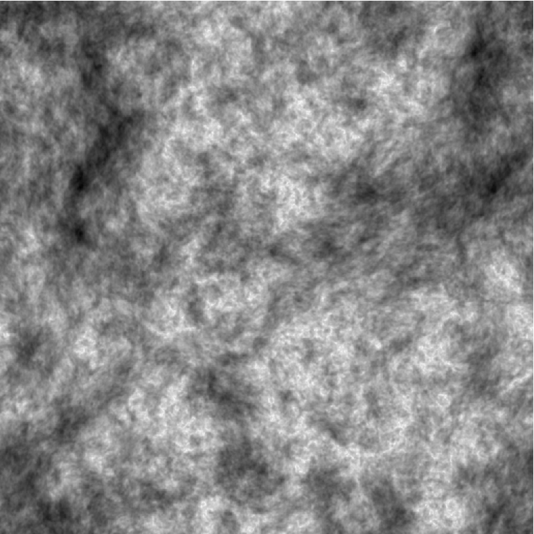
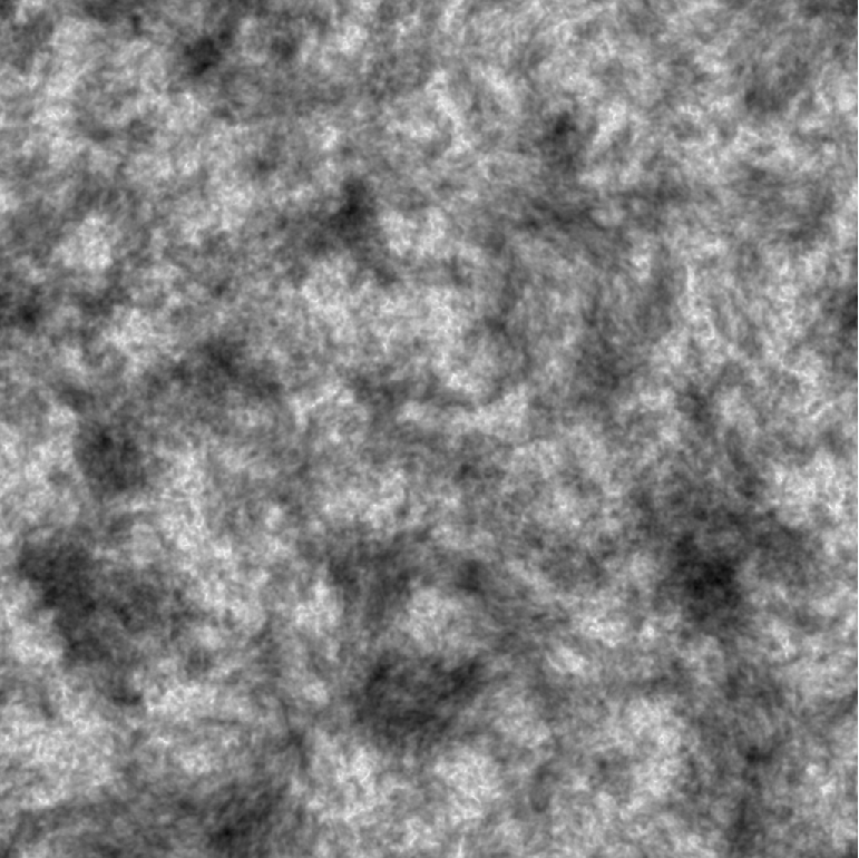
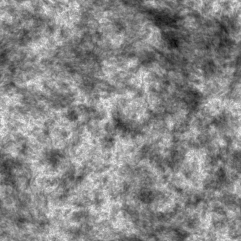
For visualization of a Gaussian velocity whose covariance mimics inertial range turbulence, see Figure 1.

Figure 1. Snapshots in space at various times of a white-in-time Gaussian random velocity.

The homogenous Gaussian forcing $f_{t}:=f(x,t)$ is taken independent and defined by the covariance

$$\mathbb{E}\left[{f}(x,t){f}(x^{\prime},t^{\prime})\right]=F(x-x^{\prime})\delta(t-t^{\prime}).$$ (8)

Equation (1) is interpreted in the Stratonovich sense (denoted by $\circ$). The Itô form of equation (1) reads

$${\rm d}\theta_{t}^{\kappa}+{\rm d}u_{t}\cdot\nabla\theta_{t}^{\kappa} =\tfrac{1}{2}D(0):\nabla\otimes\nabla\theta_{t}^{\kappa}{\rm d}t+\kappa\Delta\theta_{t}^{\kappa}\ {\rm d}t+{\rm d}f_{t},$$ (9)

$$\theta_{t}^{\kappa}|_{t=0} =\theta_{0}.$$ (10)

The setup is called the Kraichnan model [Kraichnan68, FGV01, CFG08], reviewed in the wonderful lecture notes of Gawȩdzki [gawedzki1997turbulence, gawedzki1999easy, gawedzki2000soluble]. The velocity field can be written concretely as

$${\rm d}u_{t}(x)=\sum_{n=0}^{\infty}\sigma^{(n)}(x){\rm d}W^{(n)}_{t},\qquad\sigma^{(n)}(x):=\sqrt{\lambda_{n}}e_{n}(x),$$ (11)

where $W^{(n)}_{t}$ are independent one-dimensional Brownian motions and where $\lambda_{n}$ and $e_{n}(x)$ for $n=0,1,2,\dots$ are the eigenvalues and eigenfunctions of the positive, trace-class operator with kernel $D(x-x^{\prime})$ acting on $L^{2}(\mathbb{R}^{d},\mathbb{R}^{d})$. The kernel $D$ can be represented by

$$D^{ij}(x-x^{\prime})=\sum_{n=0}^{\infty}\sigma^{(n)}_{i}(x)\sigma^{(n)}_{j}(x^{\prime}).$$ (12)

Here the $\sigma^{(n)}$ are divergence-free vector fields since $D$ is divergence-free in each index. We will consider a model of the viscous–convective range for the scalar in which the velocity if Lipschitz, the so-called Batchelor regime for the model. The rough version of the model, mimicking a turbulent inertial range, has been a topic of a great deal of study [BGK98, LJR02, LJR04]. See also discussion in [eyink2022kraichnan, eyink2022high] regarding the effects of molecular fluctuations on the phenomenology of scalar advection below the viscous–convective range. In this work, we will specialize our covariance even further

Definition 1 (Self-similar isotropic covariance).

We say $D$ is self-similarly isotropic if it takes the form

$$D(0)-D(r) =D_{1}\left[I+\left(\frac{2}{d-1}\right)\left(I-\hat{r}\otimes\hat{r}\right)\right]|r|^{2}$$ (13)

for some constant $D_{1}>0$ and $D(0)=D_{0}I$ for $D_{0}>0$.

Example 1.

A prototypical example of a self-similarly isotropic random field arises in the following context. Consider a Gaussian field defined by the covariance

$$D_{ij}(r)=\bar{D}_{0}\int\frac{P_{ij}(k)}{(|k|+m^{2})^{(d-\zeta)/2}}{\rm e}^{ik\cdot r}{\rm d}k$$ (14)

where $\zeta>2$. The constant $m$ is an infrared cutoff for the velocity and $P_{ij}$ is the projection onto the divergence-free subspace. At short distances, one can compute that

$$D_{0}\delta^{ij}-D^{ij}(r)=D_{1}\left[\delta^{ij}+\left(\frac{2}{d-1}\right)\left(\delta^{ij}-\hat{r}^{i}\hat{r}^{j}\right)\right]r^{2}+O((m|r|)^{2}),$$ (15)

where

$${D}_{0}=\frac{\mkern 1.5mu\overline{\mkern-1.5muD\mkern-1.5mu}\mkern 1.5mu_{0}}{m^{2}}\frac{d-1}{d(4\pi)^{d/2}\Gamma\left(\frac{d+2}{2}\right)},\qquad{D}_{1}=\mkern 1.5mu\overline{\mkern-1.5muD\mkern-1.5mu}\mkern 1.5mu_{0}\frac{d-1}{(d+2)(4\pi)^{d/2}\Gamma\left(\frac{d+2}{2}\right)}.$$ (16)

Thus, taking the infrared limit $m\to 0$ gives a self-similarly isotropic random field.

The forcing in (1) is also represented by a statistically independent collection of one-dimensional independent Brownian motions $\{B^{(k)}_{t}\}_{k\in\mathbb{N}}$ and of scalar functions $\{q^{(k)}\}_{k\in\mathbb{N}}$, as

$${\rm d}f_{t}(x)=\sum_{k=0}^{\infty}q^{(k)}(x){\rm d}B^{(k)}_{t},\qquad q^{(k)}(x):=\sqrt{\mu_{k}}u_{k}(x),$$ (17)

where $B^{(k)}_{t}$ are independent Brownian motions and where $\mu_{k}$ and $u_{k}(x)$ for $k=0,1,2,\dots$ are the eigenvalues and eigenfunctions of the positive, trace-class operator with kernel $F(x-x^{\prime})$ acting on $L^{2}(\mathbb{R}^{d},\mathbb{R})$. We denote averages over the random velocity by $\mathbb{E}^{u}[\cdot]$, averages over the forcing by $\mathbb{E}^{f}[\cdot]$ and averages over both simply by $\mathbb{E}[\cdot]$.

In this note, we are interested in the mixing properties of Gaussian random fields. In the context of stochastic transport, exponential mixing estimates have been obtained in [BBPS22, BBPS21] for velocities generated by the stochastic Navier-Stokes equations, in [GY21] for Kraichnan-type models with noise satisfying a general Hörmander condition, and in [BCZG23, Cooperman22] for alternating shear flows with either random phases or random switching times. On the other hand, deterministic constructions of exponentially mixing flows can be found in [ELM23, ACM19, YZ17, EZ19]. The purpose of this note is to give a new and simple, yet explicit and quantitative proof of mixing for (1). Our main result, which quantifies mixing in terms of negative Sobolev norms [oakley2021mix], is

Theorem 1 (Scalar Mixing Identity).

Suppose that $D$ is an incompressible, homogeneous and self-similarly isotropic correlation function (13). Then we have the identity

$$\mathbb{E}\|\theta^{\kappa}_{t}\|_{\dot{H}^{-s}}^{2}={\rm e}^{-\lambda_{d,s}t}\|\theta_{0}\|_{\dot{H}^{-s}}^{2}+\frac{F_{s}}{\lambda_{d,s}}\Big{(}1-{\rm e}^{-\lambda_{d,s}t}\Big{)}-\kappa\int_{0}^{t}{\rm e}^{-\lambda_{d,s}(t-\tau)}\mathbb{E}\|\theta_{\tau}^{\kappa}\|_{\dot{H}^{1-s}}^{2}{\rm d}\tau$$ (18)

where ${\lambda}_{d,s}:=2D_{1}s(d-2s)$ and $F_{s}=\sum_{k=0}^{\infty}\|q^{(k)}\|_{\dot{H}^{-s}}^{2}$.

In particular, when there is no forcing ($q^{(k)}\equiv 0$), we obtain mixing in expectation $\mathbb{E}\ \|\theta_{t}\|_{H^{-s}}^{2}\to 0$ with an exponentially fast rate, with rate uniform in the diffusivity $\kappa$. The identity (18) may look surprising, since mixing estimates typically require to pay derivatives on the initial datum to gain decay. This would indeed be the case for a pathwise estimate, since in general solutions can mix and unmix and hence a time reversal in a $\dot{H}^{-s}\mapsto\dot{H}^{-s}$ would be in conflict with a decay estimate. The point is that (18) is an identity in expectation, hence the possible realizations in which growth and unmixing happen are averaged out.

2. Adapted Mixing Identity and Proof of Theorem 1

We establishes an exact balance of “mixing norms” tailored in a particular way to the covariance of the velocity field $D$. A similar identity appeared recently in the work of Coghi and Maurelli, where it was used to improve the local wellposedness theory for stochastic Euler with multiplicative noise [coghi2023existence].

Lemma 1 (Adapted Mixing Identity).

Let $D$ be homogenous and divergence-free. Suppose that a function $G:\mathbb{R}^{d}\to\mathbb{R}$ can be found to satisfy

$$\big{(}D(0)-D(r)\big{)}:\nabla_{r}\otimes\nabla_{r}G=-\lambda G,$$ (19)

pointwise in space for some $\lambda\in\mathbb{R}$. Then the solution $\theta_{t}^{\kappa}$ of (1) satisfies the following “mixing” identity,

$$\mathbb{E}\ \langle\theta_{t}^{\kappa},G*\theta_{t}^{\kappa}\rangle_{L^{2}}={\rm e}^{-\lambda t}\langle\theta_{0},G*\theta_{0}\rangle_{L^{2}}+\frac{1}{\lambda}F_{G}\Big{(}1-{\rm e}^{-\lambda t}\Big{)}-\kappa\int_{0}^{t}{\rm e}^{-\lambda(t-\tau)}\mathbb{E}\langle\nabla\theta_{\tau}^{\kappa},G*\nabla\theta_{\tau}^{\kappa}\rangle_{L^{2}}{\rm d}\tau$$ (20)

where the source is $F_{G}:=2\int_{\mathbb{R}^{d}}G(r)F(r){\rm d}r$.

Proof of Lemma 1.

First, by definition, we have

$$\langle\theta_{t}^{\kappa},G*\theta_{t}^{\kappa}\rangle_{L^{2}}=\int_{\mathbb{R}^{d}}\theta_{t}^{\kappa}(x)\int_{\mathbb{R}^{d}}G(r)\theta_{t}^{\kappa}(x+r){\rm d}r{\rm d}x.$$ (21)

Recall (leaving the sum over $n$ implicit) that

$${\rm d}\theta_{t}^{\kappa}+\sigma^{(n)}\cdot\nabla\theta_{t}^{\kappa}{\rm d}W^{(n)}_{t} =\tfrac{1}{2}D(0):\nabla\otimes\nabla\theta_{t}^{\kappa}{\rm d}t+\kappa\Delta\theta_{t}^{\kappa}{\rm d}t+q^{(n)}{\rm d}B^{(n)}_{t},$$

$${\rm d}(G*\theta_{t}^{\kappa})+G*(\sigma^{(n)}\cdot\nabla\theta_{t}^{\kappa}){\rm d}W^{(n)}_{t} =\tfrac{1}{2}D(0):\nabla\otimes\nabla(G*\theta_{t}^{\kappa}){\rm d}t+\kappa\Delta(G*\theta_{t}^{\kappa}){\rm d}t+(G*q^{(n)}){\rm d}B^{(n)}_{t}.$$

Thus, by Ito’s product rule, we have

$${\rm d}\left(\theta_{t}^{\kappa}\ G*\theta_{t}^{\kappa}\right) =(G*\theta_{t}^{\kappa})\ {\rm d}\theta_{t}^{\kappa}+\theta_{t}^{\kappa}\ {\rm d}(G*\theta_{t}^{\kappa})+{\rm d}[\theta_{t}^{\kappa},G*\theta_{t}^{\kappa}]$$

$$=-(G*\theta_{t}^{\kappa})\sigma^{(n)}\cdot\nabla\theta_{t}^{\kappa}{\rm d}W^{(n)}_{t}-\theta_{t}^{\kappa}(G*(\sigma^{(n)}\cdot\nabla\theta_{t}^{\kappa})){\rm d}W^{(n)}_{t}$$

$$\qquad+(G*\theta_{t}^{\kappa})q^{(n)}{\rm d}B^{(n)}_{t}+\theta_{t}^{\kappa}(G*q^{(n)}){\rm d}B^{(n)}_{t}$$

$$\qquad\ \ +\tfrac{1}{2}(G*\theta_{t}^{\kappa})D(0):\nabla\otimes\nabla\theta_{t}^{\kappa}{\rm d}t+\tfrac{1}{2}\theta_{t}^{\kappa}D(0):\nabla\otimes\nabla(G*\theta_{t}^{\kappa}){\rm d}t$$

$$\qquad\quad+\kappa\theta_{t}^{\kappa}\Delta(G*\theta_{t}^{\kappa})+\kappa(G*\theta_{t}^{\kappa})\Delta\theta_{t}^{\kappa}+\sigma^{(n)}\cdot\nabla\theta_{t}^{\kappa}\ (G*(\sigma^{(n)}\cdot\nabla\theta_{t}^{\kappa})){\rm d}t.$$

Upon integrating over space and using the fact that mollification is self-adjoint in $L^{2}$, we have

$${\rm d}\langle\theta_{t}^{\kappa},G*\theta_{t}^{\kappa}\rangle_{L^{2}} =-2\langle G*\theta_{t}^{\kappa},\sigma^{(n)}\cdot\nabla\theta_{t}^{\kappa}\rangle_{L^{2}}{\rm d}W^{(n)}_{t}+2\langle\theta_{t}^{\kappa},(G*q^{(n)})\rangle_{L^{2}}{\rm d}B^{(n)}_{t}$$

$$\qquad+(D(0)+\kappa I):\langle\theta_{t}^{\kappa},\nabla\otimes\nabla(G*\theta_{t}^{\kappa})\rangle_{L^{2}}$$

$$\qquad\quad-\int_{\mathbb{R}^{d}}\int_{\mathbb{R}^{d}}\theta_{t}^{\kappa}(x)\sigma^{(n)}(x)\otimes\sigma^{(n)}(x+r):\nabla\otimes\nabla(G*\theta_{t}^{\kappa}){\rm d}x{\rm d}r{\rm d}t$$

$$\qquad\quad\quad+2\int_{\mathbb{R}^{d}}\int_{\mathbb{R}^{d}}G(r)F(x,x+r){\rm d}r{\rm d}x$$

$$=-2\langle G*\theta_{t}^{\kappa},\sigma^{(n)}\cdot\nabla\theta_{t}^{\kappa}\rangle_{L^{2}}{\rm d}W^{(n)}_{t}+2\langle\theta_{t}^{\kappa},(G*q^{(n)})\rangle_{L^{2}}{\rm d}B^{(n)}_{t}$$

$$\qquad+\int_{\mathbb{R}^{d}}(D(0)-D(r)+\kappa I):\langle\theta_{t}^{\kappa}(\cdot),G(r)(\nabla\otimes\nabla\theta_{t}^{\kappa})(\cdot+r)\rangle_{L^{2}}{\rm d}r{\rm d}t$$

$$\qquad\quad\quad+2\int_{\mathbb{R}^{d}}\int_{\mathbb{R}^{d}}G(r)F(x,x+r){\rm d}r{\rm d}x.$$

Thus, we obtain

$${\rm d}\langle\theta_{t}^{\kappa},G*\theta_{t}^{\kappa}\rangle_{L^{2}} =-2\langle G*\theta_{t}^{\kappa},\sigma^{(n)}\cdot\nabla\theta_{t}^{\kappa}\rangle_{L^{2}}{\rm d}W^{(n)}_{t}+2\langle\theta_{t}^{\kappa},(G*q^{(n)})\rangle_{L^{2}}{\rm d}B^{(n)}_{t}$$

$$\qquad+\int_{\mathbb{R}^{d}}(D(0)-D(r)+\kappa I):(\nabla_{r}\otimes\nabla_{r}G)(r)\langle\theta_{t}^{\kappa}(\cdot),\theta_{t}^{\kappa}(\cdot+r)\rangle_{L^{2}}{\rm d}r{\rm d}t$$

$$\qquad\quad\quad+2\int_{\mathbb{R}^{d}}\int_{\mathbb{R}^{d}}G(r)F(x,x+r){\rm d}r{\rm d}x.$$

In the above calculation, we repeatedly made use of the fact that the $\sigma^{(n)}$ are divergence-free, integrated by parts and changed some $x$ to $r$ derivatives. Appealing to the defining equation (19) for the kernel $G$, we find

$${\rm d}\langle\theta_{t}^{\kappa},G*\theta_{t}^{\kappa}\rangle_{L^{2}} =-\lambda\langle\theta_{t}^{\kappa},G*\theta_{t}^{\kappa}\rangle_{L^{2}}-2\langle G*\theta_{t}^{\kappa},\sigma^{(n)}\cdot\nabla\theta_{t}^{\kappa}\rangle_{L^{2}}{\rm d}W^{(n)}_{t}+2\langle\theta_{t}^{\kappa},(G*q^{(n)})\rangle_{L^{2}}{\rm d}B^{(n)}_{t}+F_{G}$$

$$\qquad+\kappa\langle\Delta\theta_{t}^{\kappa},G*\theta_{t}^{\kappa}\rangle_{L^{2}},$$ (22)

where we have introduced the notation $F_{G}$ from the statement of the lemma. The result follows upon taking expectation, using the mean zero property of the martingale term and subsequently integrating. ∎

We now demonstrate a solution $G$ to (19) if it covariance function is self-similarly isotropic.

Lemma 2.

Suppose that $D$ is self-similarly isotropic. Then for any $s\in(0,d/2)$, the Riesz potential

$$G(r)=I_{s}(|r|),\qquad I_{s}(\rho)=\frac{1}{c_{d,s}}\frac{1}{\rho^{d-2s}},\qquad c_{d,s}=\pi^{d/2}2^{2s}\frac{\Gamma(s)}{\Gamma((d-2s)/2)}$$ (23)

solves equation (19) with $\lambda=2D_{1}s(d-2s)$.

Proof of Lemma 2.

We will prove something more general here by studying instead the covariance

$$D(0)-D(r) =D_{1}\left[I+\left(\frac{\zeta}{d-1}\right)\left(I-\hat{r}\otimes\hat{r}\right)\right]|r|^{\zeta}$$ (24)

with the statement of the lemma following as a corollary with $\zeta=2$. Let $z=|r|$. We seek a radial kernel $G(r):=\mathcal{G}(z)$. On such a function, we have

$$\nabla_{r}\otimes\nabla_{r}{G} =\nabla_{r}\otimes(\hat{r}\mathcal{G}^{\prime}(z))=\frac{1}{z}(I-\hat{r}\otimes\hat{r})\mathcal{G}^{\prime}(z)+\hat{r}\otimes\hat{r}\mathcal{G}^{\prime\prime}(z).$$

Note that $(I-\hat{r}\otimes\hat{r}):I=(I-\hat{r}\otimes\hat{r}):(I-\hat{r}\otimes\hat{r})=d-1$ so

$$\big{(}D(0)-D(r)\big{)}:(I-\hat{r}\otimes\hat{r}) =(d-1+\zeta)D_{1}|r|^{\zeta},$$

$$\big{(}D(0)-D(r)\big{)}:\hat{r}\otimes\hat{r} =D_{1}|r|^{\zeta}.$$

Thus we have

$$\big{(}D(0)-D(r)\big{)}:\nabla_{r}\otimes\nabla_{r}\mathcal{G} =D_{1}\Big{[}((d-1)+\zeta)z\mathcal{G}^{\prime}(z)+z^{2}\mathcal{G}^{\prime\prime}(z)\Big{]}z^{\zeta-2}.$$

Thus, equating this to $-\lambda\mathcal{G}$, we find that the kernel must solve

$$z^{2}\mathcal{G}^{\prime\prime}(z)+((d-1)+\zeta)z\mathcal{G}^{\prime}(z)+\frac{\lambda}{D_{1}}z^{2-\zeta}\mathcal{G}(z)=0.$$ (25)

We seek a solution of the type $\mathcal{G}(z)=z^{\alpha}\ln^{\beta}(z)$. Demanding the ansatz be a solution, we require

$$0 =\Bigg{[}\alpha^{2}+\Big{(}d+\zeta-2\Big{)}\alpha+\frac{\lambda}{D_{1}}z^{2-\zeta}\Bigg{]}\ln^{2}(z)+\beta\Big{(}d+\zeta-2+2\alpha\Big{)}\ln(z)+\beta(\beta-1).$$

Note that for this ansatz to be a solution, we require $\beta=0$ or $\beta=1$. Thus, we have the cases

1. If $\lambda=0$, then

   $$\alpha=2-d-\zeta,\qquad\beta=0,$$ (26)

   giving a statistically conserved quantity.

2. If $\beta=0$ and $\lambda\neq 0$ then

   $$\zeta=2,\qquad\alpha=-\frac{d}{2}\pm\sqrt{\left(\frac{d}{2}\right)^{2}-\frac{\lambda}{D_{1}}},$$ (27)

   provided that $\tfrac{\lambda}{D_{1}}\leq\left(\frac{d}{2}\right)^{2}$.

3. If $\beta=1$ then

   $$\zeta=2,\qquad\alpha=-\frac{d}{2},\qquad\frac{\lambda}{D_{1}}=\left(\frac{d}{2}\right)^{2}.$$ (28)

The stated conclusion follows easily as a special case of (b). ∎

Recall the following characterization of the $H^{-s}$ semi-norm

Lemma 3 ([Silvestre07, Landkof72]).

Let $d\geq 2$, $s\in(0,d/2)$. Then $\langle h,I_{s}*h\rangle_{L^{2}}=\|h\|_{\dot{H}^{-s}}^{2}$ where $I_{s}$ is the Riesz potential.

With this, Theorem 1 follows immediately from Lemmas 1, 2 and 3.

2.1. Two-particle dispersion

We now show that similar arguments as those used in Lemma 1 can be used to prove a kind of decay estimate for the law of the two-point Lagrangian flow associated to (1), i.e.

$${\rm d}X_{t}(x)=\sum_{n=0}^{\infty}\sigma^{(n)}(X_{t}(x))\circ{\rm d}W_{t}^{(n)}\qquad{\rm d}X_{t}(y)=\sum_{n=0}^{\infty}\sigma^{(n)}(X_{t}(y))\circ{\rm d}W_{t}^{(n)}\,,$$ (29)

with $X_{0}(x)=x,X_{0}(y)=y$. Since the velocity field is spatially homogeneous, we need only study the law $\mu_{t}=\mathrm{Law}(R_{t}({r}))$ of the separation between particles $R_{t}({r})=X_{t}(x)-X_{t}({y})$ with $r=x-y$. Using the spatial homogeneity of the velocity field $u$, one can check that $\mu_{t}$ is a solution of the following PDE

$$\partial_{t}\mu_{t}=\left(D(0)-D(r)\right):\nabla_{r}\otimes\nabla_{r}\mu_{t}\,,$$ (30)

with $\mu_{0}=\delta_{r}$. Given the above characterisation of $\mu_{t}$, we have the following result.

Proposition 1.

Assume there exists a $G$ as in the statement of Lemma 1. Then, we have

$$\int_{\mathbb{R}^{d}}G(\bar{r})\,\mathrm{d}\mu_{t}(\bar{r})={\rm e}^{-\lambda t}G(r)\,.$$ (31)

Proof.

The proof follows directly by testing (30) with $G$, integrating by parts using the fact that $D$ is divergence-free, and then using the definition of $G$. ∎

If $D$ is self-similarly isotropic, in view of Lemma 2, this means that for any $s\in(0,d/2)$, we have

$$\mathbb{E}[|X_{t}(x)-X_{t}(y)|^{2s-d}]={\rm e}^{-\lambda_{d,s}t}|x-y|^{2s-d},\qquad\lambda_{d,s}/D_{1}=2s(d-2s).$$ (32)

Thus, we obtain exact decay laws for (inverse) particle dispersion, capturing the average dispersion. In the case $s=0$, this relation becomes the statistical conservation law $\mathbb{E}[|X_{t}(x)-X_{t}(y)|^{-d}]=|x-y|^{-d}$ derived in the works [falkovich2013single, zel1984kinematic]. This fact can be understood as akin to the statement that in a given, linear, isotropic and incompressible velocity field, the average $\fint_{S^{d-1}}|X_{t}(x)-X_{t}(x+r)|^{-d}{\rm d}\omega(\hat{r})$ is a constant of motion. See the work of Frishman et al [frishman2015statistical].

3. Top Lyapunov exponent in the Kraichnan model

In this section, we present explicitly computed the Lyapunov exponents of the Lagrangian flow associated to (1). This expression for the Lyapunov exponents for first derived by Le Jan in [LJ85] in his study of isotropic Brownian flows. For completeness, we present this calculation for the leading exponent below.

Proposition 2.

Consider the Lagrangian flow $\varphi_{t}(x)$ associated to (1), i.e. the following Stratonovich SDE

$${\rm d}\varphi_{t}(x)=\sum_{n=0}^{\infty}\sigma^{(n)}(\varphi_{t}(x))\circ{\rm d}W_{t}^{(n)}\,,$$ (33)

with $\varphi_{t}(x)=x$. Furthermore, assume that $D$ is self-similarly isotropic in the sense of Definition 1. Then

$$\log(\lVert D\varphi_{t}\rVert)=dD_{1}t+M_{t},$$ (34)

where $M_{t}$ is the martingale defined by (42). The top Lyapunov exponent, defined almost surely, is

$$\lambda_{1}=\lim_{t\to\infty}\frac{\log(\lVert D\varphi_{t}\rVert)}{t}=dD_{1}.$$ (35)

Proof.

Let us define by $A_{t,x}:=(D\varphi_{t})(x)$. It is straightforward to check that

$${\rm d}A_{t,x}=\sum_{n=0}^{\infty}(D\sigma^{(n)})(\varphi_{t}(x))\cdot A_{t,x}{\rm d}W_{t}^{(n)}\,.$$ (36)

Indeed, since $\sigma^{(n)}$ are divergence-free, the Itô and Stratonovich form of SDE (33) coincide. Pick $v\in\mathbb{S}^{d-1}$ and define $v_{t,x}:=A_{t,x}v$. We then have that

$${\rm d}v_{t,x}=\sum_{n=0}^{\infty}(D\sigma^{(n)})(\varphi_{t}(x))\cdot v_{t,x}\,{\rm d}W_{t}^{(n)}\,.$$ (37)

Applying Itô’s formula, we obtain

$${\rm d}|v_{t,x}|^{2}=\sum_{n=0}^{\infty}|(D\sigma^{(n)})(\varphi_{t}(x))\cdot v_{t,x}|^{2}\,dt+2\sum_{n=0}^{\infty}\langle v_{t,x},(D\sigma^{(n)})(\varphi_{t}(x))\cdot v_{t,x}\rangle\,{\rm d}W_{t}^{(n)}\,.$$ (38)

Note that the drift term in the above expression can be simplified as follows

$$\sum_{n=0}^{\infty}|(D\sigma^{(n)})(\varphi_{t}(x))\cdot v_{t,x}|^{2}= \sum_{n=0}^{\infty}\sum_{i=1}^{d}\left|\sum_{j=1}^{d}\partial_{j}\sigma^{(n)}_{i}v_{t,x}^{j}\right|^{2}=\sum_{n=0}^{\infty}\sum_{i=1}^{d}\sum_{j,k=1}^{d}\partial_{j}\sigma^{(n)}_{i}\partial_{k}\sigma^{(n)}_{i}v_{t,x}^{j}v_{t,x}^{k}$$

$$= \langle v_{t,x},C\cdot v_{t,x}\rangle\,,$$ (39)

with the matrix $C$ given by $C_{jk}(x):=\sum_{i=1}^{d}\left.\partial_{x_{j}}\partial_{x_{k}^{\prime}}D^{ii}(x-x^{\prime})\right|_{x=x^{\prime}}\,.$ Using the expression for $D$ given by (13), we obtain $\partial_{x_{j}}\partial_{x_{k}^{\prime}}D^{ii}(x-x^{\prime})=2D_{1}\delta_{jk}\left(\frac{d+1}{d-1}-\frac{2}{d-1}\delta_{ik}\right)\,.$ Using the above, (38) reduces to

$${\rm d}|v_{t,x}|^{2}=2D_{1}(d+2)|v_{t,x}|^{2}\,dt+2\sum_{n=0}^{\infty}\langle v_{t,x},(D\sigma^{(n)})(\varphi_{t}(x))\cdot v_{t,x}\rangle\,{\rm d}W_{t}^{(n)}\,.$$ (40)

Applying Itô’s formula to the above expression again, we arrive at

$${\rm d}\log|v_{t_{x}}|= \frac{1}{2}{\rm d}\log|v_{t,x}|^{2}=D_{1}(d+2)\,dt-\frac{1}{|v_{t,x}|^{4}}\sum_{n=0}^{\infty}\left|\langle v_{t,x},(D\sigma^{(n)})(\varphi_{t}(x))\cdot v_{t,x}\rangle\right|^{2}\,dt+dM_{t}\,,$$ (41)

where the martingale term $M_{t}$ is given by

$$M_{t}=\int_{0}^{t}\frac{1}{|v_{t,x}|^{2}}\sum_{n=0}^{\infty}\langle v_{t,x},(D\sigma^{(n)})(\varphi_{t}(x))\cdot v_{t,x}\rangle\,{\rm d}W_{t}^{(n)}\,.$$ (42)

We first simplify the drift term in (41) as follows

$$\sum_{n=0}^{\infty}\left|\langle v_{t,x},(D\sigma^{(n)})(\varphi_{t}(x))\cdot v_{t,x}\rangle\right|^{2} =\sum_{n=0}^{\infty}\left|\sum_{j,k=1^{d}}v_{t,x}^{k}\partial_{j}\sigma^{(n)}_{k}v_{t,x}^{j}\right|^{2}=\sum_{n=0}^{\infty}\sum_{j,k,\ell,m=1}^{d}v_{t,x}^{k}v_{t,x}^{\ell}\partial_{j}\sigma^{(n)}_{k}\partial_{\ell}\sigma^{(n)}_{m}v_{t,x}^{j}v_{t,x}^{m}\,.$$

Note now that $\sum_{n=0}^{\infty}\partial_{j}\sigma^{(n)}_{k}\partial_{\ell}\sigma^{(n)}_{m}=\left.\partial_{x_{j}}\partial_{x_{\ell}^{\prime}}D^{km}(x-x^{\prime})\right|_{x=x^{\prime}}\,.$ Using (13) again, we obtain

$$\partial_{x_{j}}\partial_{x_{\ell}^{\prime}}D^{km}(x-x^{\prime})= 2D_{1}\left(\delta_{km}\delta_{j\ell}\left(\frac{d+1}{d-1}\right)-\frac{1}{d-1}(\delta_{kj}\delta_{m\ell}+\delta_{mj}\delta_{k\ell})\right)\,.$$ (43)

From (41), we obtain ${\rm d}\log|v_{t_{x}}|=D_{1}d\,{\rm d}t+{\rm d}M_{t}\,,$ whence (34) follows. For (35), we note that

$$\mathbb{E}(M_{t}^{2})=\sum_{n=0}^{\infty}\int_{0}^{t}\mathbb{E}\left(\frac{1}{|v_{t,x}|^{4}}|\langle v_{t,x},(D\sigma^{(n)})(\varphi_{t}(x))\cdot v_{t,x}\rangle|^{2}\right)\,{\rm d}t=2D_{1}t.$$ (44)

It follows then that $t^{-1}M_{t}$ is a supermartingale, and so by Doob’s martingale convergence theorem and the above bound, it converges almost surely to $0$. This clearly implies (35), since for any $v\in\mathbb{S}^{d-1}$, we have

$$\lim_{t\to\infty}\frac{1}{t}\log|v_{t_{x}}|=D_{1}d\,.$$

This completes the proof. ∎

Acknowledgements. We thank G. Eyink, A. Frishman and S. Punshon-Smith for useful discussions. The research of MCZ was partially supported by the Royal Society URF\R1\191492 and EPSRC Horizon Europe Guarantee EP/X020886/1. The research of TDD was partially supported by the NSF DMS-2106233 grant and NSF CAREER award #2235395. The research of RSG was partially supported by the Deutsche Forschungsgemeinschaft through the SPP 2410/1 Hyperbolic Balance Laws in Fluid Mechanics: Complexity, Scales, Randomness.