Bounding and estimating MCMC convergence rates using common random number simulations

Abstract

This paper explores how and when to use common random number (CRN) simulation to evaluate MCMC convergence rates. We discuss how CRN simulation is closely related to theoretical convergence rate techniques such as one-shot coupling and coupling from the past. We present conditions under which the CRN technique generates an unbiased estimate of the Wasserstein distance between two random variables. We also discuss how unbiasedness of the Wasserstein distance between two Markov chains over a single iteration does not extend to unbiasedness over multiple iterations. We provide an upper bound on the Wasserstein distance of a Markov chain to its stationary distribution after $N$ steps in terms of averages over CRN simulations. We apply our result to a Bayesian regression Gibbs sampler.

1 Introduction

Markov chain Monte Carlo (MCMC) algorithms are often used to simulate from a stationary distribution of interest (see e.g. [5]). One of the primary questions when using these Markov chains is, after how many iterations is the distribution of the Markov chain sufficiently close to the stationary distribution of interest, i.e. when should actual sampling begin [20]. The number of iterations it takes for the distribution of the Markov chain to be sufficiently close to stationarity is called the burn-in period. Various informal methods are available for estimating the burn-in period, such as effective sample size estimation, the Gelman-Rubin diagnostic, and visual checks using traceplots or autocorrelation graphs [40, 21, 13, 36]. However, none of these methods provide a formal estimate of the distance between the distribution of the Markov chain and the stationary distribution.

From a theoretical perspective, distance to stationarity is traditionally measured in terms of total variation distance (e.g. [47, 37]), though more recently the Wasserstein distance has been considered [17, 29, 35, 24]. However, finding upper bounds on either distance can be quite difficult to establish [20, 15], and if an upper bound is known, it is usually based on complicated problem-specific calculations [34, 24, 45, 43]. This motivates the desire to instead estimate convergence bounds from actual simulations of the Markov chain, which we consider here.

One common method for generating upper bounds on the Wasserstein distance is through a contraction condition (see Definition 2.1). This can often be established using the common random number (CRN) simulation technique, i.e. using the same random variables to simulate two copies of a Markov chain with different initial values (see Section 2). Estimating Markov chain convergence rates using CRN simulation was first proposed in [25] to find estimates of mixing times in total variation distance; see also [11, 22]. This approach falls under the general framework of “auxiliary simulation” [9], i.e. using extra preliminary Markov chain runs to estimate the convergence time needed in the final run. More recently, [2] showed how CRN simulation could be used for estimating an upper bound on the Wasserstein distance (their Proposition 3.1), and provided useful applications of the CRN method to high-dimensional and tall data (their Section 4). Simulation using the CRN technique is useful since for random variables under certain conditions it is an unbiased estimate of the Wasserstein distance (see equation 4) and for Markov chains under certain conditions it is a conditionally unbiased estimate of the Wasserstein distance (see equation 12). It was shown in [18] that simulated Euclidean distance generated using the CRN technique is an unbiased estimate of the Wasserstein distance when the random transformation is an increasing function of the uniform random variable (see propositions 3.1 and 3.2 below).

In this paper, in Theorem 3.3 below, we generalize the result of [18] and conclude that the CRN technique generates an unbiased estimate of the Wasserstein distance whenever the intervals over which the transformation of a random variable in $\mathbb{R}$ are increasing and decreasing are the same. This theorem should help establish whether the CRN technique is optimal for simulating the Wasserstein distance, or if another simulation technique such as [30, 9, 48, 27, 51, 3] is merited. Within the context of Markov chains, unbiasedness is only proven over a single iteration. We show how it is more difficult to extend over multiple iterations in Section 3.3.

Then, in Theorem 4.4 below, we provide an estimated upper bound in terms of CRN simulation on the Wasserstein distance between a Markov chain and the corresponding stationary distribution when only the unnormalized density of the stationary distribution is known. We apply this theorem (Section 5) to a Bayesian regression Gibbs sampler with semi-conjugate priors.

This paper is organized as follows. In Section 2, we present definitions and notation. We also discuss the relationship between the closely related notions of coupling from the past, one-shot coupling, and the CRN technique. In Section 3, we present a set of random functions (of real-valued random variables) that will generate unbiased estimates of the Wasserstein distance when the CRN technique is used. In Section 4, we establish convergence bounds of a Markov chain to its corresponding stationary distribution using the CRN technique when the initial distribution is not in stationarity. Finally, in Section 5, we apply our Theorem 4.4 to a Bayesian regression Gibbs sampler example. The code used to generate all of the tables and calculations can be found at github.com/sixter/CommonRandomNumber.

2 Background

2.1 Distances between measures

Let $X,Y$ be two random variables on the measure space $(\mathcal{X},\mathcal{F},\lambda)$ and $\pi,\nu$ be two probability measures. We denote the law of $X$ as $\mathcal{L}(X)$ and $d:\mathcal{X}\times\mathcal{X}\to\mathbb{R}_{+}$ as a metric function. When not specified, the distance, $d$, refers to the Euclidean distance. The Wasserstein distance between two probability measures $\pi$ and $\nu$ is the infimum of the expected distance between $X$ and $Y$ over all joint distributions with marginals $\mathcal{L}(X)=\pi$ and $\mathcal{L}(Y)=\nu$, $W_{d}(\pi,\nu)=\inf_{J(X,Y)}E[d(X,Y)]$ where $J(X,Y)$ is the set of all joint distributions where $\mathcal{L}(X)=\pi$ and $\mathcal{L}(Y)=\nu$. The maximal coupling of the Wasserstein distance is the random variable pair $(X_{M},Y_{M})$ that minimizes the expected distance, $W_{d}(\pi,\nu)=d(X_{M},Y_{M})$ and $\mathcal{L}(X_{M})=\pi,\mathcal{L}(Y_{M})=\nu$. Total variation is defined as $||\pi-\nu||_{TV}=\sup_{A\in\mathcal{F}}|\pi(A)-\nu(A)|$.

2.2 Essential supremum and infimum

Let $f:\mathcal{X}\to\mathbb{R}$ be a function on the measure space $(\mathcal{X},\mathcal{F},\lambda)$. The essential supremum is the smallest value $a\in\mathbb{R}$ such that $\lambda(x\mid f(x)<a)=1$. More formally, $ess\sup_{x}f(x)=\{\inf_{a\in\mathbb{R}}a\mid\lambda(x\mid f(x)>a)=0\}$. The essential infimum is likewise the largest value $a\in\mathbb{R}$ such that $\lambda(x\mid f(x)>a)=1$. Or, $ess\inf_{x}f(x)=\{\sup_{a\in\mathbb{R}}a\mid\lambda(x\mid f(x)<a)=0\}$ [32].

2.3 Iterative function systems: Backward and forward process

Define a Markov chain $\{X_{n}\}_{n\geq 1}$ on a complete separable metric space $(\mathcal{X},d)$ such that $X_{n}=f_{\theta_{n}}(X_{n-1})$, where $\{\theta_{n}\}_{n\geq 1}$ are i.i.d. random variables. The set of possible functions $f_{\theta_{1}},f_{\theta_{2}},\ldots$ is called an iterated function system. Any time homogeneous Markov chain can be represented as an iterated function system [46].

The iterated function system defines the forwards and backwards processes. The forwards process, $\{X_{n}\}_{n\geq 1}$, which is a Markov chain, is defined as follows,

$$X_{n}=f_{\theta_{n}}(f_{\theta_{n-1}}(\ldots f_{\theta_{1}}(X_{0})))$$

The backwards process, $\{\tilde{X}_{n}\}_{n\geq 1}$, which is not a Markov chain but tends to converge pointwise to a limit, is defined as follows,

$$\tilde{X}_{n}=f_{\theta_{1}}(f_{\theta_{2}}(\ldots f_{\theta_{n}}(X_{0})))$$

Figure 1 graphs the forward and backward process of an autoregressive process using the same random mappings. The point towards which the backwards process converges is itself random.

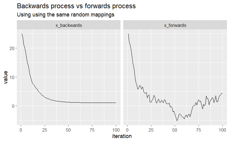
Figure 1: The backwards, $\{\tilde{X}_{n}\}_{n\geq 1}$, and forwards, $\{X_{n}\}_{n\geq 1}$, process of the autoregressive normal system where $X_{n},\tilde{X}_{n}$ are simulated using the same random mappings, $X_{n}=0.9X_{n-1}+Z_{n},Z_{n}\sim N(0.1)$ and $X_{0}=25$.

Despite the difference in behaviour of the two processes, the marginal distributions of the forward and backward processes are the same, $X_{n}\overset{d}{=}\tilde{X}_{n}$, so the backwards process is sometimes used when studying convergence properties of the forwards Markov chain [12, 46, 45].

2.4 Convergence of forward and backward processes

When studying the convergence rates of iterated random functions, we are typically interested in establishing a contraction condition. The ‘vanilla’ contraction condition, sometimes referred to as global average [46] or strongly [45] contractive, is defined as the supremum over all $x$ of the expected Lipschitz constant.

Definition 2.1 (Global average contraction condition).

There exists a $D\in(0,1)$ such that for $n\geq 0$,

$$\sup_{x,x^{\prime}}E[d(X_{n},X^{\prime}_{n})\mid X_{n-1}=x,X^{\prime}_{n-1}=x^{\prime}]\leq Dd(x,x^{\prime})$$

Modifications to the above contraction condition have been widely studied and can be found in [46, 45, 23, 16, 28, 12].

When establishing convergence results using contraction conditions, the backwards process (called coupling from the past when the state space is finite [33]) is usually applied while one-shot coupling associated with the forwards process is less often applied. See [45, 46, 12] for examples of applications of coupling from the past and [23, 43, 31, 17, 26] for examples of applications of one-shot coupling. Coupling from the past and one-shot coupling are seldom mentioned in the same texts with the exception of [22]. While the approach for generating contraction rate bounds is different, these two techniques actually generate equivalent results and are both, at their foundation, applications of the CRN technique.

In particular, if two forward processes $X_{N},X^{\prime}_{N}$ are simulated using the CRN technique (i.e., $X_{n}=f_{\theta_{n}}(X_{n-1})$ and $X^{\prime}_{n}=f_{\theta_{n}}(X^{\prime}_{n-1})$ for $n\in\mathbb{N}$) then the expected distance between the $n$th iteration of the two forward processes is equal to the expected distance between the $n$th and $n+1$th iteration of the backwards process, $\tilde{X}_{n}$.

$$E[d(X_{n},X^{\prime}_{n})\mid X_{0}=x,X^{\prime}_{0}=f_{\theta_{n+1}}(x)]$$

$$=E[d[f_{\theta_{n}}(f_{\theta_{n-1}}(\ldots f_{\theta_{1}}(x)\ldots)),f_{\theta_{n}}(f_{\theta_{n-1}}(\ldots f_{\theta_{1}}(f_{\theta_{n+1}}(x))\ldots))]\mid X_{0}=x,X^{\prime}_{0}=f_{\theta_{n+1}}(x)]$$

$$=E[d[f_{\theta_{1}}(f_{\theta_{2}}(\ldots f_{\theta_{n}}(x)\ldots)),f_{\theta_{1}}(f_{\theta_{2}}(\ldots f_{\theta_{n}}(f_{\theta_{n+1}}(x))\ldots))]\mid\tilde{X}_{0}=x]$$

$$=E[d(\tilde{X}_{n},\tilde{X}_{n+1})\mid\tilde{X}_{0}=x]$$

2.5 Common random numbers

Previously we defined the CRN technique to setting $\theta_{n}=\theta^{\prime}_{n}$, i.e. using the same seed to simulate both Markov chains. This is the intuitive definition of CRN for application [11, 2, 19]. However, we will first restrict our discussion to defining the CRN technique based on using uniform random variables as the common random number. Later on, we will discuss how expanding the definition of the CRN technique from a uniform random variable to $\theta_{n}$ affects the optimality of the CRN technique.

3 Using the common random number technique as a conditionally unbiased estimate of the Wasserstein distance

3.1 Common random number applied to a random variable

Suppose $X,Y$ are two random variables such that their marginal distributions can be represented as the inverse cumulative distribution function (CDF) of a uniform random variable. That is $X=F^{-1}_{X}(U)$ where $F^{-1}_{X}$ is the inverse cumulative distribution function of the marginal and $U\sim Unif(0,1)$. Most joint probability spaces can be represented as such [18, 41, 50, 49]. A sufficient condition is that $F_{X}$ be continuous (see exercise 1.2.4 of [14]).

We first define CRN to jointly setting $(X,Y)=(F^{-1}_{X}(U),F^{-1}_{Y}(U))$ [18]. We will call this definition the InvCDF-CRN (inverse CDF - common random number). The InvCDF-CRN is the joint distribution that minimizes the expected square distance between two random variables. That is, the InvCDF-CRN solves the Monge-Kanterovich problem when $d(x,y)=(x-y)^{2}$ (see Section 2.3.1 of [22]).

This definition stems from the following proposition which says that the maximum supermodular transform between the joint distribution of $(X,Y)$ is attained when $(X,Y)=(F^{-1}_{X}(U),F^{-1}_{Y}(U))$.

Proposition 3.1 (Theorem 2 of [7] and Proposition 2.1 of [18]).

Suppose that $\psi:\mathcal{X}\times\mathcal{X}\to\mathbb{R}$ is a supermodular function ($\psi(x_{1},y_{1})+\psi(x_{2},y_{2})\geq\psi(x_{1},y_{2})+\psi(x_{2},y_{1})$ when $x_{1}\leq x_{2}$ and $y_{1}\leq y_{2}$) and a right continuous function and that $U\sim Unif(0,1)$. Then for random variables $X,Y$ defined on $\mathcal{X}$,

$$\sup_{J(X,Y)}E[\psi(X,Y)]=E[\psi(F^{-1}_{X}(U),F^{-1}_{Y}(U))]$$

where $J(X,Y)$ is the set of all joint distributions of $(X,Y)$ with marginals $\mathcal{L}(X),\mathcal{L}(Y)$.

Some examples of supermodular functions are $\psi(xy)=xy,(x+y)^{2},\min\{x,y\},f(x-y)$ where $f$ is concave and continuous, $-|x-y|^{p},p\geq 1$ (Section 4 of [7]). Proposition 3.1 is consistent with Theorem 2.9 of [42].

In this paper we focus on the supermodular function $\psi(x,y)=xy$. If the CRN generates the supremum expectation for the function $\psi(x,y)=xy$ (i.e., $\sup_{J(X,Y)}E[XY]=E[F^{-1}_{X}(U)F^{-1}_{Y}(U)]$), then the CRN generates the supremum expectated covariance as follows:

$$\sup_{J(X,Y)}Cov(X,Y) =\sup_{J(X,Y)}E[XY]-E[X]E[Y]$$ (1)

$$=F^{-1}_{X}(U)F^{-1}_{Y}(U)-E[F^{-1}_{X}(U)]E[F^{-1}_{Y}(U)]$$ (2)

$$=Cov(F^{-1}_{X}(U),F^{-1}_{Y}(U))$$ (3)

By the same reasoning, if the CRN generates the supremum expectation for the function $\psi(x,y)=xy$, then the CRN generates the infimum expected Euclidean distance or Wasserstein distance as follows:

$$W_{d}(\mathcal{L}(X),\mathcal{L}(Y)) \coloneqq\inf_{J(X,Y)}E[(X-Y)^{2}]$$ (4)

$$=E[X^{2}]+E[Y^{2}]-\sup_{J(X,Y)}E[XY]$$ (5)

$$=E[(F^{-1}_{X}(U)-F^{-1}_{Y}(U))^{2}]$$ (6)

See Section 2 of [22] and [18] for more details on how the CRN technique and Wasserstein distance are related.

3.2 Common random number in a Markov chain setting.

Within the context of a Markov chain we define the CRN technique as follows. Let $\{X_{n}\}_{n\geq 1}$ be a Markov chain such that $X_{n}$ is defined as an iterated function system and $X_{n}=f_{\theta_{n}}(X_{n-1})=f(\theta_{n},X_{n-1})$ where $\theta_{1},\theta_{2}\ldots$ are i.i.d. random variables. We assume that $\theta$ can be constructed from a uniform random variable, $\theta=F^{-1}_{\theta}(U)$, $U\sim Unif(0,1)$. Note that if $\theta\in\mathbb{R}^{p}$ is a vector of independent random variables, then each coordinate can be constructed from a uniform random variable $\vec{\theta}=F^{-1}_{\vec{\theta}}(\vec{U})$ where $U_{i}\sim Unif(0,1)$ are i.i.d. (this is consistent with equation 3 of [18]). When used in simulation, the CRN technique visibly shows how two copies of a Markov chain converge. See figure 2 for an example of two autoregressive processes that converge.

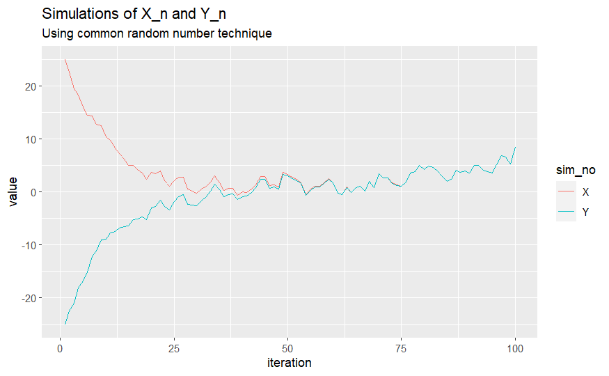
Figure 2: Two copies of the autoregressive process where $X_{n},Y_{n}$ are simulated using CRN, $X_{n}=0.9X_{n-1}+Z_{n},Z_{n}\sim N(0,1)$, and $X_{0}=25,Y_{0}=-25$

Next, we extend Proposition 3.1 to non-decreasing functions of uniform random variables. We denote $X_{1}=f(F^{-1}_{\vec{\theta}}(\vec{U}),x)$ and $Y_{1}=f(F^{-1}_{\vec{\theta}}(\vec{V}),y)$, where $U,V\sim Unif(0,1)$. The result follows for $n\geq 1$ recursively.

Proposition 3.2 (Proposition 2.2 of [18]).

Define $X_{1}=f(\theta_{U},x)$ and $Y_{1}=f(\theta_{V},y)$ be random functions where $\theta_{U}=F^{-1}_{\theta}(U)$, $\theta_{V}=F^{-1}_{\theta}(V)$ and $U,V\sim Unif(0,1)$. If for fixed $x,y$, $f(\cdot,x),f(\cdot,y)$ are non-decreasing continuous functions with finite second mean ($E[f(\cdot,y)^{2}]<\infty$ and $E[f(\cdot,x)^{2}]<\infty$) then

$$\sup_{J(U,V)}E[f(\theta_{U},x)f(\theta_{V},y)]$$ (7)

is attained by setting $U=V$.

We relaxed the assumption that $f(\cdot,x)$ be increasing to assuming that $f(\cdot,x)$ is non-decreasing. The relaxed assumption generates the same conclusion since $\psi(f(\cdot,x),f(\cdot,x))$ remains supermodular if $\psi$ is supermodular and $f(\cdot,x),f(\cdot,y)$ are non-decreasing (which is required in the proof of Proposition 2.2 of [18]). Note, for example that the distribution function $F^{-1}$ in Proposition 2.1 of [18] is a non-decreasing function, not a strictly increasing function.

Similar to Proposition 3.1, the supremum covariance (equation 1) and infimum Euclidean distance (equation 4) are attained when $U=V$.

In practise, however, $f(\theta,x)$ and $f(\theta,y)$ are not always non-decreasing functions with respect to $\theta$. Rather, the following theorem shows that the supremum is attained when $U=V$ if the functions $f(\theta,x)$ and $f(\theta,y)$ are both increasing and decreasing for the same values of $\theta\in\mathbb{R}$.

Theorem 3.3.

Define $X_{1}=f(\theta_{U},x)$ and $Y_{1}=f(\theta_{V},y)$ be random functions where $\theta_{U}=F^{-1}_{\theta}(U)$ and $U,V\sim Unif(0,1)$. Define the sets $A=(I_{x}\cap I_{y})\cup(D_{x}\cap D_{y})$ where

• $I_{x}$ is the area over which $f(\theta,x)$ is a non-decreasing function. That is, $\theta_{0}\in I_{x}$ if there exists $\epsilon_{0}>0$ such that for $0<\epsilon<\epsilon_{0}$, $f(\theta_{0},x)\leq f(\theta_{0}+\epsilon,x)$

• $D_{x}$ is the area over which $f(\theta,x)$ is a non-increasing function. That is, $\theta_{0}\in D_{x}$ if there exists $\epsilon_{0}>0$ such that for $0<\epsilon<\epsilon_{0}$, $f(\theta_{0},x)\geq f(\theta_{0}+\epsilon,x)$

with equivalent notation for $I_{y},D_{y}$.

If for fixed $x,y$, $f(\theta,x)$ and $f(\theta,y)$ have bounded variation and have finite second moments (i.e., $E_{\theta}[f(\theta,y)^{2}],E_{\theta}[f(\theta,x)^{2}]<\infty$), then

• If $P(A)=1$ (the intervals of positive measure over which $\theta$ is increasing and decreasing on $f(\cdot,x)$ and $f(\cdot,y)$ are the same),

  $$W_{d}(\mathcal{L}(X_{1}),\mathcal{L}(Y_{1}))=E[(f(\theta_{U},x)-f(\theta_{U},y))^{2}]$$ (8)

  i.e. $(f(\theta_{U},x)-f(\theta_{U},y))^{2}$ is an unbiased estimate of $W_{d}(L(X_{1}),L(Y_{1}))$.

• If $P(A)=0$ (that is the function $f(\cdot,x)$ is increasing and $f(\cdot,y)$ is decreasing over the same intervals of positive measure or vice versa),

  $$W_{d}(\mathcal{L}(X_{1}),\mathcal{L}(Y_{1}))=E[(f(\theta_{1-U},x)-f(\theta_{U},y))^{2}]$$ (9)

  i.e. $(f(\theta_{1-U},x)-f(\theta_{U},y))^{2}$ is an unbiased estimate of $W_{d}(L(X_{1}),L(Y_{1}))$.

• If $0<P(A)<1$ (there are intervals of positive measure over which $\theta$ is increasing on $f(\cdot,x)$ and decreasing on $f(\cdot,y)$ or vice versa),

  $$\inf_{J(\theta_{U},\theta_{V})}E[(f(\theta_{U},x)-f(\theta_{V},y))^{2}]$$ (10)

  $$\in E[f(\theta_{U},x)^{2}]+E[f(\theta_{V},y))^{2}]+[E[f(\theta_{U},x)f(\theta_{U},y)],E[f(\theta_{U},x)f(\theta_{U},y)]+e]$$ (11)

  Where $e=E[(f(\theta_{1-U},x)-f(\theta_{U},x))f(\theta_{U},y)1_{A^{C}}]$

The proof is in Section 6.

The set $A$ is simpler to visualize. It is the values of $\theta$ for which either both $f(\theta,x)$ and $f(\theta,y)$ are increasing or decreasing for fixed $x,y$. See figure 3 for an example.

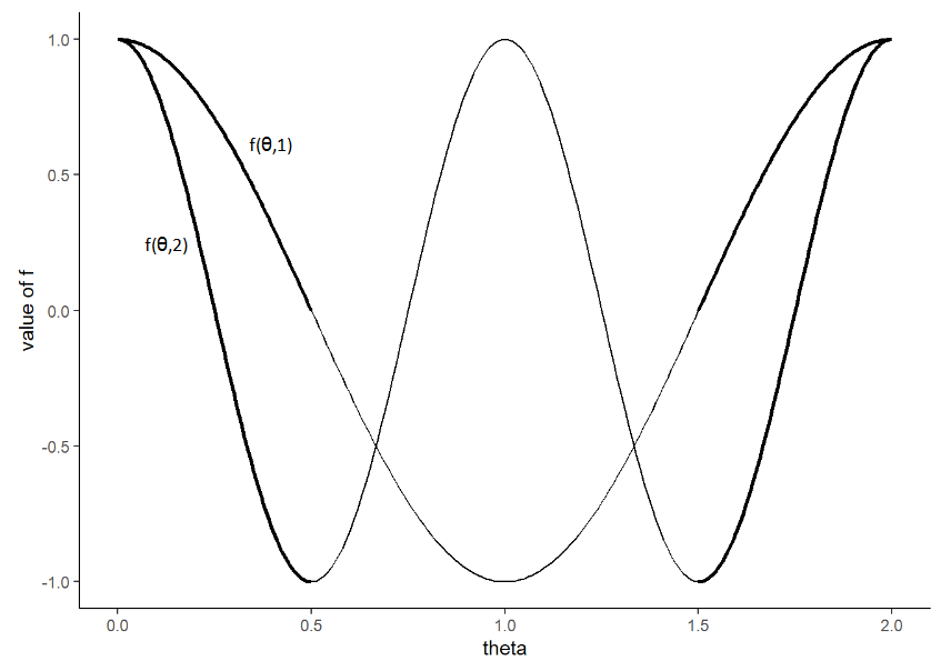
Figure 3: Denote $f(\theta,x)=\cos(\pi x\theta)$. The above graphs two functions: $f(\theta,1)=\cos(\pi\theta)$ and $f(\theta,2)=\cos(2\pi\theta)$. The set $A$ in this case is the value of $\theta$ where the function is bold. That is, $A=(0,0.5)\cup(1.5,2)$.

3.3 Conditionally unbiased estimates of the Wasserstein distance

Denote $X_{n}=f(\theta_{n},X_{n-1})$ and $Y_{n}=f(\theta^{\prime}_{n},Y_{n-1})$ where $\theta_{n},\theta^{\prime}_{n}\in\mathbb{R}$ are random variables. Theorem 3.3 implies that if $P(A)=1$ for all $X_{n-1}=x$ and $Y_{n-1}=y$, then applying the CRN technique to simulate $E[(X_{n}-Y_{n})^{2}]$ will generate conditionally unbiased estimates of the Wasserstein distance. That is, for two copies of a Markov chain, $X_{n}$ and $Y_{n}$, that were simulated by CRN ($X_{n}=f(\theta_{n},X_{n-1})$ and $Y_{n}=f(\theta_{n},Y_{n-1})$), the Wasserstein distance will be conditionally unbiased on $X_{n-1}$ and $Y_{n-1}$ as follows:

$$W_{d}(\mathcal{L}(X_{n}),\mathcal{L}(Y_{n})\mid X_{n-1}=x,Y_{n-1}=y) \coloneqq\inf_{J(X_{n},Y_{n})}E[(X_{n}-Y_{n})^{2}\mid X_{n-1}=x,Y_{n-1}=y]$$ (12)

$$=E[(f(\theta_{n},X_{n-1})-f(\theta_{n},Y_{n-1}))^{2}\mid X_{n-1}=x,Y_{n-1}=y]$$ (13)

This is the maximal coupling for the Wasserstein distance given the previous iteration.

Remark.

Note that Markov chains that satisfy $P(A)=1$ for all $X_{n-1}=x$ and $Y_{n-1}=y$ and are simulated by CRN may not be unconditionally unbiased. Unconditional unbiasedness is defined as follows for $X_{0}=x$ and $Y_{0}=y$:

$$W_{d}(\mathcal{L}(X_{n}),\mathcal{L}(Y_{n}))=E[(f(\theta_{n},f(\theta_{n-1},\ldots f(\theta_{1},x)\ldots))-f(\theta_{n},f(\theta_{n-1},\ldots f(\theta_{1},y)\ldots)))^{2}]$$

To illustrate our point, fix $n=2$ and initial values $X_{0}=x,Y_{0}=y$. Suppose that $W_{d}(\mathcal{L}(X_{2}),\mathcal{L}(Y_{2}))=E[(f(\theta_{2},f(\theta_{1},x))-f(\theta_{2},f(\theta_{1},y)))^{2}]$ where $\theta_{1}\perp\!\!\!\perp\theta_{2}$. Then

$$W_{d}(\mathcal{L}(X_{2}),\mathcal{L}(Y_{2})) \coloneqq\inf_{J(\theta_{1},\theta^{\prime}_{1})\times J(\theta_{2},\theta^{\prime}_{2})}E[(f(\theta_{2},f(\theta_{1},x))-f(\theta^{\prime}_{2},f(\theta^{\prime}_{1},y)))^{2}]$$

$$=\inf_{J(\theta_{1},\theta_{1}^{\prime})}E[(f(\theta_{2},f(\theta_{1},x))-f(\theta_{2},f(\theta^{\prime}_{1},y)))^{2}]$$ by assumption

However, the function $f(\theta_{2},\cdot)$ may be increasing for $f(\theta_{1},x)$ and decreasing for $f(\theta_{1},y)$ (or vice versa), which by Theorem 3.3 means that the function might not generate the infimum expectation.

Remark.

Even if a Markov chain does not present itself as conditionally unbiased it might still be conditionally unbiased under different function construction. This is because the CRN technique depends on the function $f$. To quote [48] “In most […] scenarios the user must construct a coupling tailored to the problem at hand.” For example, if $X_{1}$ and $Y_{1}$ have continuous distribution functions, then they can be written as transformations of the uniform distribution and thus a common random number that generates the maximum covariance exists. Generating such a function $g$ such that $X_{n}=g(U),U\sim Unif(0,1)$ may not be easy to calculate, however. For example, the Metropolis Hastings algorithm does not appear to converge in expectation when the heuristic algorithm for using the common random number on the proposal and accept/reject random variables is used [10]. Figure 4 shows that when we apply the heuristic algorithm on the CRN technique of a Metropolis algorithm, sample mean convergence is bounded away from $0$. In [30], asymptotically optimal estimates using a variation of the CRN are provided for the Metropolis-Hastings algorithm when the target distribution is elliptical normal.

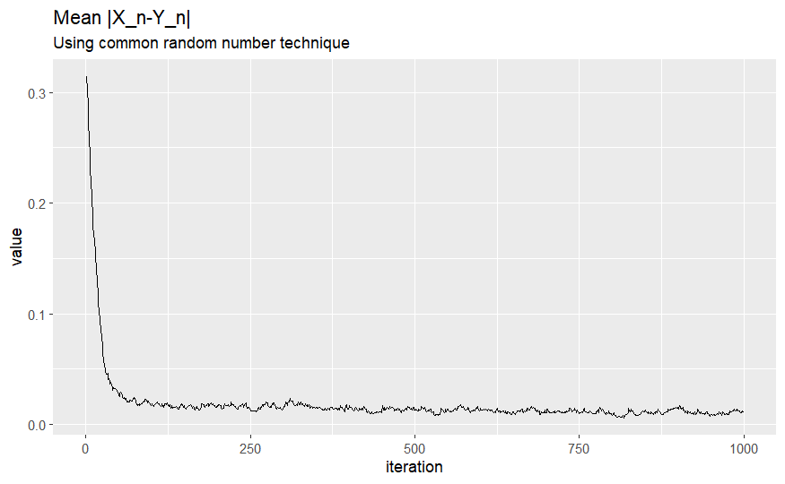
Figure 4: We apply a Metropolis algorithm on the unnormalized ($c>0$) target density, $\pi(x)=cg(x)$ where $g(x)=x^{3}\sin y^{4}\cos y^{5}$ with proposal distribution $N(X_{n-1},0.01)$. The next iteration can be written as a function of $Z_{n}\sim N(0,1)$ and $U_{n}\sim Unif(0,1)$ as follows $X_{n}=(X_{n-1}+0.1Z_{n})I\{U_{n}<(X_{n-1}+0.1Z_{n})/X_{n-1}\}+X_{n-1}I\{U_{n}\geq(X_{n-1}+0.1Z_{n})/X_{n-1}\}$. When we use CRN on $Z_{n}$ and $U_{n}$ to simulate $X_{n}$ and $Y_{n}$, $|X_{n}-Y_{n}|$ does not converge even though the Wasserstein distance does converge.

The following two examples use Theorem 3.3 to show that the CRN technique generates conditionally unbiased estimates of the Wasserstein distance.

Example 3.1 (Random logistic map).

Define $X_{n}\in[0,1]$ to be a random logistic map. That is, $X_{n}=f(\theta_{n},X_{n-1})=4\theta_{n}X_{n-1}(1-X_{n-1})$ and $\theta_{n}\sim Beta(a+1/2,a-1/2)$ for $a>1/2$. Since $f(\theta_{n},X_{n-1})$ is a non-decreasing function of $\theta_{n}$ for all values of $X_{n-1}\in[0,1]$, then by Theorem 3.3 the CRN technique provides simulated estimates of the Euclidean distance that are conditionally unbiased to the Wasserstein distance. That is, if $\hat{X}_{n}$ and $\hat{Y}_{n}$ are CRN simulations of the random logistics map then $W_{d}(\mathcal{L}(X_{n}),\mathcal{L}(Y_{n}))=E[(\hat{X}_{n}-\hat{Y}_{n})^{2}]$

See figure 5 for an example of two random logistic map processes that converge. See Section 7.4 of [45] for theoretical convergence diagnostics in total variation distance and example 2 of [29] for upper bounds in Wasserstein distance as a function of total variation distance.

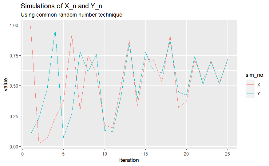
Figure 5: Two copies of the random logistic map where $X_{n},Y_{n}$ are simulated using CRN, $X_{n}=4\theta_{n}X_{n-1}(1-X_{n-1}),\theta\sim Beta(1.5,0.5)$, and $X_{0}=0.99,Y_{0}=0.1$

Example 3.2.

Define $X_{n}\in[-1,1]$ to be a Markov chain such that $X_{n}=f(\theta_{n},X_{n-1})=\sin[(1-|X_{n-1}|)\cos(\theta_{n})]$ and $\theta_{n}\sim Unif(-\pi/2,3\pi/2)$. Since $f(\theta_{n},X_{n-1})$ is increasing and decreasing over the same regions of $\theta$ for fixed $X_{n-1},Y_{n-1}\in[-1,1]$, then by Theorem 3.3 the CRN technique provides simulated estimates of the Euclidean distance that are conditionally unbiased to the Wasserstein distance.

Figure 6 provides an example of copies of this Markov chain converging when the CRN technique is used. Figure 7 shows that for initial values $X_{0}=0.75$ and $Y_{0}=0.05$ the functions $f(X_{0},\theta)$ and $f(Y_{0},\theta)$ are both increasing and decreasing over the same regions of $\theta$.

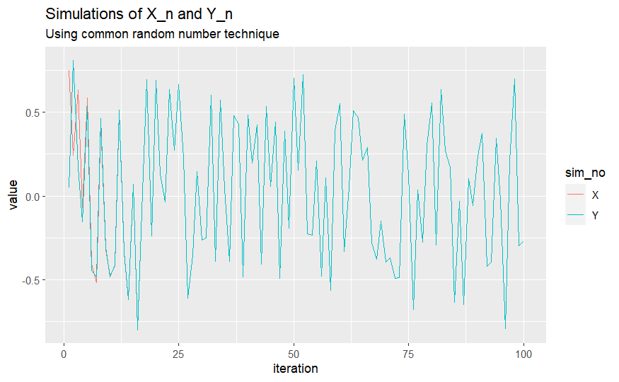
Figure 6: Two copies of a Markov chain $X_{n}=f(\theta_{n},X_{n-1})=\sin[(1-|X_{n-1}|)\cos(\theta_{n})]$ where $\theta_{n}\sim Unif(-\pi/2,3\pi/2)$. $X_{n},Y_{n}$ are simulated using CRN, with initial values and $X_{0}=0.75,Y_{0}=0.05$

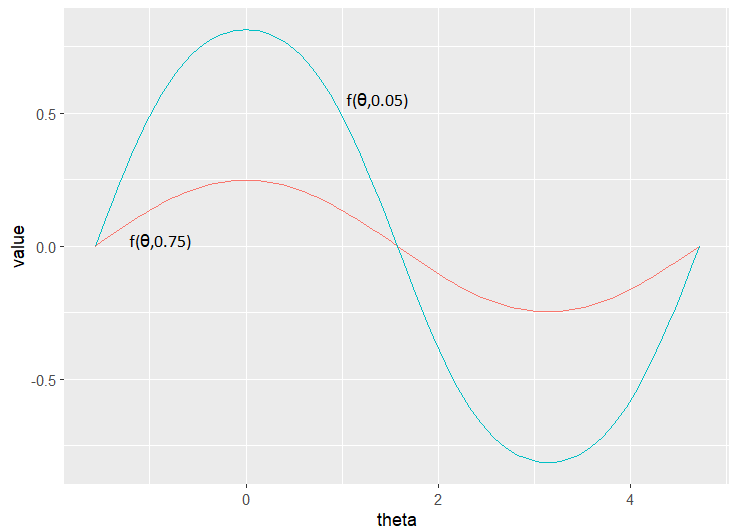
Figure 7: Denote $f(\theta,x)=\sin[(1-|x|)\cos(\theta)]$. The above graphs two functions: $f(\theta,0.75)=\sin[0.25\cos(\theta)]$ and $f(\theta,0.05)=\sin[0.95\cos(\theta)]$. Note that both functions are decreasing over the same region, $\theta=(0,\pi)$.

Finally, note that Theorem 3.3 is only applicable for $\theta\in\mathbb{R}$. Further research needs to be done to extend the above results to $\theta\in\mathbb{R}^{d}$. However, we believe that a proof can be established using Proposition 3.2 and assuming that $f(\theta,x)$ is of bounded Arzel$\grave{a}$-variation (see Definition 3.2.1 of [4]). If a function defined in $\mathbb{R}^{d}$ is of bounded Arzel$\grave{a}$-variation, then it can be written as the difference of two coordinate-wise increasing functions (see Theorem 3.4.1 of [4]) where Proposition 3.2 can then be applied. Example 3.3 is a Markov chain of Dirichlet process means where $\theta\in\mathbb{R}^{2}$ and $f(\theta,x)$ is not always an increasing function of $\theta$, so none of the theorems in this text apply. The CRN technique still appears to generate converging Markov chains, however (see figure 8).

Example 3.3 (Dirichlet process means).

Define $X_{n}\in[0,1]$ to be a Markov chain of Dirichlet process means. That is $X_{n}=f(\theta_{n},Z_{n},X_{n-1})=(1-\theta_{n})Z_{n}+\theta_{n}X_{n-1}$ and $\theta_{n}\sim Beta(a,1)$ for $a>0$ and $Z_{n}\sim N(0,1)$. In this case $(\theta_{n},Z_{n})\in\mathbb{R}^{2}$, so Theorem 3.3 does not apply. Further, since $f(\theta_{n},Z_{n},X_{n-1})$ may not necessarily be an increasing function of $(\theta_{n},Z_{n})$, Proposition 3.2 also does not apply. The Markov chain of Dirichlet process means still seems to converge when the CRN technique is used. See figure figure 8 for an example of two Markov chains with Dirichlet processes means that converge. See section 7 of [38] for theoretical convergence diagnostics.

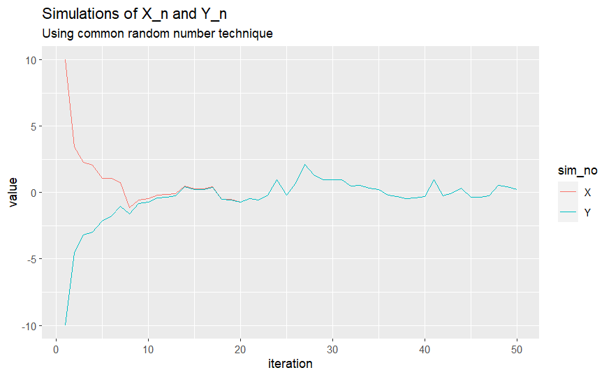
Figure 8: Two copies of a Markov chain with Dirichlet process means where $X_{n},Y_{n}$ are simulated using CRN, $X_{n}=(1-\theta_{n})Z_{n}+\theta_{n}Z_{n-1},\theta\sim Beta(1.5,1),Z_{n}\sim N(0,1)$, and $X_{0}=10,Y_{0}=-10$

4 Common random number as a method of simulating Markov chain convergence rates

We propose estimating the Wasserstein distance between the $n$th iteration of a Markov chain $X_{n}$ and the corresponding stationary distribution $X_{\infty}$ through simulation using the CRN technique. Our method is outlined in Theorem 4.4. Using CRN simulation as a convergence diagnostic tool was first discussed in [25] for bounding total variation distance.

Before providing a method for simulating an upper bound on $E[|X_{n}-X_{\infty}|]$, we must first provide a method of bounding the expected distance between two copies of a Markov chain ($E[|X_{n}-Y_{n}|]$) and their corresponding expected distance to stationarity, ($E[|X_{n}-X_{\infty}|]$). To do so, we will first define rejection sampling and separation distance and how they are related.

Definition 4.1 (Rejection sampling).

Suppose that we have a target distribution $\pi$, which we want to sample from, but is difficult to do, and we have a proposal distribution $\nu$ that is easier to sample from. Suppose also that $\pi<<\nu$ (i.e., $\pi(A)=0\implies\nu(A)=0$, where $A\in\mathcal{F}$) and $K\nu(x)\geq\pi(x),x\in\mathcal{X}$ for some known $K$. To generate a random variable $X_{\pi},\mathcal{L}(X_{\pi})=\pi$ we do the following,

1. Sample $X\sim\nu$ and $U\sim Unif(0,1)$ independently.

2. If $U\leq\frac{\pi(X)}{K\nu(X)}$ then accept $X$ as a draw from $\pi$. Otherwise reject $X$ and restart from step 1.

Lemma 4.1 (Rejection sampler rejection rate).

Denote the event $A=\{X\text{ is accepted as a draw from }\pi\}$ in the rejection sampler algorithm defined above. The rejection rate denoted as $r$ is as follows where $K=ess\sup_{x\in\mathcal{X}}\frac{\pi(x)}{\nu(x)}$.

$$r(\pi,\nu)=1-P(A)=1-\frac{1}{K}$$

Proof.

See Section 11.2.2 of [39]. ∎

We further define the separation distance on the continuous state space $\mathcal{X}$ as follows. Separation distance was first defined in [1] for discrete state spaces. As far as we know, separation distance was only recently defined on a continuous state space in [8]. We use the definition of separation distance defined in [8] where the density functions are known.

Definition 4.2 (Separation distance (Remark 5 of [8])).

Let $\nu$ and $\pi$ be two density functions defined on the same measure space $(\mathcal{X},\mathcal{F},\lambda)$ such that $\nu<<\pi$. The separation distance is,

$$s=s(\pi,\nu)=ess\sup_{x}\left(1-\frac{\nu(x)}{\pi(x)}\right)$$

It turns out that the separation distance and the rejection rate of the rejection sampler are the same.

Lemma 4.2.

Let $\nu$ and $\pi$ be two positive density functions defined on the same measure space $(\mathcal{X},\mathcal{F},\lambda)$. If $\nu$ is the proposal distribution and $\pi$ is the target distribution in a rejection sampler, then the rejection rate equals the separation distance,

$$s(\pi,\nu)=r(\pi,\nu)$$

Proof.

$$s(\pi,\nu) =ess\sup_{x\in\mathcal{X}}\left(1-\frac{\nu(x)}{\pi(x)}\right)=1-ess\inf_{x\in\mathcal{X}}\frac{\nu(x)}{\pi(x)}=1-\frac{1}{ess\sup_{x\in\mathcal{X}}\frac{\pi(x)}{\nu(x)}}=1-\frac{1}{K}=r(\pi,\nu)$$

∎

Now that we have defined separation distance and the rejection rate of the rejection sampler, we can apply upper bounds on the distance to stationarity as follows. The use of rejection sampling to generate an upper bound on the expected distance between a proposal distribution $\nu$ and a stationary distribution $\pi$ was inspired by [25], which used rejection sampling to generate similar upper bounds in total variation distance.

Theorem 4.3.

Let $\{X_{n}\}_{n\geq 1}$ and $\{Y_{n}\}_{n\geq 1}$ be two copies of a Markov chain in $\mathcal{X}$ with initial distribution $\mathcal{L}(X_{0})=\mu,\mathcal{L}(Y_{0})=\nu$. Let $X_{\infty}$ be the corresponding stationary random variable with distribution $\pi$ such that $\pi$ and $\nu$ are defined on the same support. Then,

$$E[|X_{n}-X_{\infty}|]\leq CE[|X_{n}-Y_{n}|]$$ (14)

Where $C=\frac{1}{1-s(\pi,\nu)}=\frac{1}{1-r(\pi,\nu)}=K$

Proof.

Let $X_{n},Y_{n}$ be two copies of the Markov chain and $A=\{\text{Accept $Y_{0}$ as a draw from }\pi\}$. Let $r(\pi,\nu)=1-P(A)$. Note that $\mathcal{L}(Y_{0}|A)=\pi$ and so, $\mathcal{L}(Y_{n}|A)=\pi$.

$$E[|X_{n}-Y_{n}|] =E[|X_{n}-Y_{n}|:A]P(A)+E[|X_{n}-Y_{n}|:A^{c}]P(A^{c})$$

$$\geq E[|X_{n}-X_{\infty}|]P(A)$$

$$\geq E[|X_{n}-X_{\infty}|]\frac{1}{K}$$

Further, $1/K=1-r(\pi,\nu)=1-s(\pi,\nu)$ and so equation 14 follows. ∎

In many cases the normalizing constant for $\pi$ is unknown. That is, we only know of a function $g(x)$ such that $cg(x)=\pi(x)$ where $c$ is unknown. In this case we must find a constant $L>0$ such that $\int_{\mathcal{X}}g(x)dx\geq L$, which implies that $c\leq\frac{1}{L}$ and

$$K\leq\frac{1}{L}\sup_{x\in\mathcal{X}}\frac{g(x)}{\nu(x)}$$ (15)

See Example 5.1 for a way of estimating $K$ when the normalizing constant of $\pi$ is unknown. In Section 5 we estimate $L$ as the integral over a bounded subset of $\mathcal{X}$, $B\subset\mathcal{X}$. That is, $L=\int_{B}g(x)dx$. [6] presents an alternative approach to estimating the rejection rate, $K$, when the normalizing constant for $\pi$ is unknown.

Next we define Algorithm 1 for generating an estimate of $\inf_{J(X_{N},Y_{N})}E[|X_{N}-Y_{N}|]$, $N\geq 1$ where $\mathcal{L}(X_{0})=\mu,\mathcal{L}(Y_{0})=\nu$. The algorithm generates a conditionally unbiased estimate of the Wasserstein distance provided the conditions in Theorem 3.3 hold. This algorithm is similar to algorithm 1 in [2].

Algorithm 1 An estimate of $E[|X_{N}-Y_{N}|]\approx\frac{1}{I}\sum_{i=1}^{I}|x_{N,i}-y_{N,i}|$ using CRN

while $i\leq I$ do

     $x_{0,i}\sim\mu$, $y_{0,i}\sim\nu$ where $x_{0,i}\perp\!\!\!\perp y_{0,i}$

     while $n\leq N$ do

         $\theta_{n}\sim\Theta$

         $x_{n,i}\leftarrow f_{\theta_{n}}(x_{n-1,i})$

         $y_{n,i}\leftarrow f_{\theta_{n}}(y_{n-1,i})$

         $n\leftarrow n+1$

     end while

     $i\leftarrow i+1$

end while

return $\frac{1}{I}\sum_{i=1}^{I}|x_{N,i}-y_{N,i}|$

Combining algorithm 1 with Theorem 4.3, we can simulate an upper bound between a Markov chain at iteration $N$, $X_{N}$, and the corresponding stationary random variable, $X_{\infty}$, as follows,

Theorem 4.4.

Suppose that the Markov chain $\{X_{n}\}_{n\geq 1}$ with stationary distribution $\mathcal{L}(X_{\infty})=\pi$ has finite second moments for all $n\geq 1$ and can be written as an iterated function system $X_{n+1}=f_{\theta_{n+1}}(X_{n})$ where ${\theta}_{n\geq 1}$ are i.i.d. random variables. Suppose further that the initial distribution of $Y$, $\mathcal{L}(Y_{0})=\nu$ is defined on the same support as $\pi$. Then,

$$E[|X_{N}-X_{\infty}|]\leq C\lim_{I\to\infty}\frac{1}{I}\sum_{i=1}^{I}|x_{N,i}-y_{N,i}|$$ (16)

Where $\frac{1}{I}\sum_{i=1}^{I}|x_{N,i}-y_{N,i}|$ is defined as in algorithm 1 and $C=\frac{1}{1-s(\pi,\nu)}=\frac{1}{1-r(\pi,\nu)}=K$.

Proof.

Fix $N\geq 1$. By the weak law of large numbers, $\lim_{I\to\infty}\frac{1}{I}\sum_{i=1}^{I}|x_{N,i}-y_{N,i}|\overset{a.s.}{=}E[|X_{N}-Y_{N}|]$. By Theorem 4.3, $E[|X_{N}-X_{\infty}|]\leq CE[|X_{N}-Y_{N}|]$ and so equation 16 follows. ∎

The consistency of $\lim_{I\to\infty}\frac{1}{I}\sum_{i=1}^{I}|x_{N,i}-y_{N,i}|$ is similarly proven in Proposition 3.1 of [2].

5 Bayesian regression Gibbs sampler example

Consider the Bayesian linear regression model with semi-conjugate priors (see chapter 5 of [36]) for which we will apply Theorem 4.4 to simulate convergence bounds on the Wasserstein distance.

Example 5.1 (Bayesian regression Gibbs sampler with semi-conjugate priors).

Suppose we have the following observed data $Y\in\mathbb{R}^{k}$ and $X\in\mathbb{R}^{k\times p}$ where

$$Y|\beta,\sigma\sim N_{k}(X\beta,\sigma^{2}I_{k})$$

for unknown parameters $\beta\in\mathbb{R}^{p},\sigma^{2}\in\mathbb{R}$. Suppose we apply the prior distributions on the unknown parameters,

• $\beta\sim N(\beta_{0},\Sigma_{\beta})$

• $\sigma^{2}\sim\text{Inv-}\chi^{2}(\upsilon_{0},c_{0}^{2})$

The joint density function is proportional to the following equation,

$$\beta,\sigma^{2}|Y\propto g(\beta,\sigma^{2})=\frac{1}{(\sigma^{2})^{(n+\upsilon_{0})/2+1}}\exp\left(-\frac{1}{2\sigma^{2}}(y-X\beta)^{T}(y-X\beta)-\frac{1}{2}(\beta-\beta_{0})^{T}\Sigma_{\beta}^{-1}(\beta-\beta_{0})-\frac{\upsilon_{0}c_{0}^{2}}{2\sigma^{2}}\right)$$ (17)

The Bayesian regression Gibbs sampler is based on the marginal posterior distributions of $\beta_{n},\sigma^{2}_{n}$ and is defined as follows.

• $\beta_{n}|\sigma_{n-1}^{2},Y\sim N(\tilde{\beta}_{\sigma^{2}_{n-1}},V_{\beta,\sigma^{2}_{n-1}})$

• $\sigma^{2}_{n}|\beta_{n},Y\sim\Gamma^{-1}\left(\frac{k+\upsilon_{0}}{2},\frac{1}{2}\left[\upsilon_{0}c_{0}^{2}+(Y-X\beta_{n})^{T}(Y-X\beta_{n})\right]\right)$

Where $V_{\beta,\sigma^{2}_{n-1}}=\left(\frac{1}{\sigma^{2}_{n-1}}X^{T}X+\Sigma_{\beta}^{-1}\right)^{-1}$ and $\tilde{\beta}_{\sigma^{2}_{n-1}}=V_{\beta,\sigma^{2}_{n-1}}\left(\frac{1}{\sigma^{2}_{n-1}}X^{T}X\hat{\beta}+\Sigma_{\beta}^{-1}\beta_{0}\right)$, and $\hat{\beta}=(X^{T}X)^{-1}X^{T}Y$. $\Gamma^{-1}(\alpha,\beta)$ represents the inverse gamma distribution.

Replacing $\beta_{n}=\tilde{\beta}_{\sigma^{2}_{n-1}}+V_{\beta,\sigma^{2}_{n-1}}^{1/2}Z_{n}$, where $Z_{n}\sim N(0,I_{p})$ into the equation for $\sigma^{2}_{n}$ we get that

$$\sigma^{2}_{n}|\sigma^{2}_{n-1},Y=\left[\frac{\upsilon_{0}c_{0}^{2}}{2}+\frac{(X\tilde{\beta}_{\sigma^{2}_{n-1}}-Y+XV_{\beta,\sigma^{2}_{n-1}}^{1/2}Z_{n})^{T}(X\tilde{\beta}_{\sigma^{2}_{n-1}}-Y+XV_{\beta,\sigma^{2}_{n-1}}^{1/2}Z_{n})}{2}\right]\frac{1}{G_{n}}$$ (18)

Where $G_{n}\sim\Gamma(\frac{k+\upsilon_{0}}{2},1)$

Lemma 5.1.

Let the proposal distribution of $\sigma^{2}_{0}$ be simulated according to an inverse gamma, $\sigma^{2}_{0}\sim\Gamma^{-1}(\alpha^{\prime},\beta^{\prime})$ where $\alpha^{\prime}=(n+\upsilon_{0})/2$ and $\beta^{\prime}=\upsilon_{0}c_{0}^{2}$. Define $f$ as the corresponding density function, $f(\sigma^{2})=\frac{\beta^{\prime\alpha^{\prime}}}{\Gamma(\alpha^{\prime})}\frac{1}{(\sigma^{2})^{\alpha^{\prime}+1}}e^{-\beta^{\prime}/\sigma^{2}}$. Then $K\geq\frac{1}{\int_{\mathcal{R}^{p}\times\mathcal{R}_{+}}g(\beta,\sigma^{2})d(\beta\times\sigma^{2})}\frac{\Gamma(\alpha^{\prime})}{\beta^{\prime\alpha^{\prime}}}$.

Proof.

Note that $g(\beta,\sigma^{2})\geq\frac{1}{(\sigma^{2})^{(n+\upsilon_{0})/2+1}}\exp\left(-\frac{\upsilon_{0}c_{0}^{2}}{\sigma^{2}}\right)=\frac{\Gamma(\alpha^{\prime})}{\beta^{\prime\alpha^{\prime}}}f(\beta,\sigma^{2})$. By equation 15 the value for $K$ follows. ∎

Lemma 5.2.

For the Bayesian regression Gibbs sampler with semi-conjugate priors, the total variation distance can be bounded by the expected distance as follows,

$$||\mathcal{L}(\sigma^{2}_{n})-\mathcal{L}(\sigma^{{}^{\prime}2}_{n})||_{TV} \leq\frac{n+\upsilon_{0}}{\upsilon_{0}c_{0}^{2}}E[|\sigma^{2}_{n}-\sigma^{{}^{\prime}2}_{n}|]$$

Proof.

For $n=N$, let $Z_{n}=Z^{\prime}_{n}$ and denote $Z_{n}=\frac{\upsilon_{0}c_{0}^{2}}{2}+\frac{(X\tilde{\beta}_{\sigma^{2}_{n-1}}-Y+XV_{\sigma^{2}_{n-1}}^{1/2}Z_{n})^{T}(X\tilde{\beta}_{\sigma^{2}_{n-1}}-Y+XV_{\sigma^{2}_{n-1}}^{1/2}Z_{n})}{2}$ so that $\sigma^{2}_{n}=Z_{n}\frac{1}{G_{n}}$ and $\sigma^{{}^{\prime}2}_{n}=W^{\prime}_{n}\frac{1}{G^{\prime}_{n}}$. In expectation, the difference between $\sigma^{2}_{n}$ and $\sigma^{{}^{\prime}2}_{n}$ are close. Denote $\Delta=W^{\prime}_{n}-Z_{n}$ and without loss of generality, $W^{\prime}_{n}>Z_{n}$

$$||\mathcal{L}(\sigma^{2}_{n})-\mathcal{L}(\sigma^{{}^{\prime}2}_{n})||_{TV}$$

$$\leq E\left[||\mathcal{L}(Z_{n}\frac{1}{G_{n}})-\mathcal{L}(W^{\prime}_{n}\frac{1}{G^{\prime}_{n}})||_{TV}\right]$$

$$=E\left[||\mathcal{L}(Z_{n}\frac{1}{G_{n}})-\mathcal{L}((Z_{n}+\Delta)\frac{1}{G^{\prime}_{n}})||_{TV}\right]$$

$$=E\left[||\mathcal{L}\left(\frac{1}{G_{n}}\right)-\mathcal{L}\left(\left(1+\frac{\Delta}{Z_{n}}\right)\frac{1}{G^{\prime}_{n}}\right)||_{TV}\right]$$ By Proposition 2.1 of [43]

$$\leq E\left[\sup_{x>0}1-\frac{\pi_{1/G_{n}}(x)}{\pi_{(1+\Delta/Z_{n})/G_{n}}(x)}\right]$$ By Proposition 2.2 of [43]

Since $G_{n}\sim\text{Gamma}(\alpha,1)$ where $\alpha=\frac{n+\upsilon_{0}}{2}$

$$\pi_{1/G_{n}}(x) \propto x^{-\alpha-1}e^{-1/x}$$

$$\pi_{(1+\Delta/Z_{n})/G_{n}}(x) \propto\frac{1}{1+\Delta/Z_{n}}\left(\frac{x}{1+\Delta/Z_{n}}\right)^{-\alpha-1}e^{-(1+\Delta/Z_{n})/x}$$

$$=(1+\Delta/Z_{n})^{\alpha}x^{-\alpha-1}e^{-(1+\Delta/Z_{n})/x}$$

So,

$$||\mathcal{L}(\sigma^{12}_{n})-\mathcal{L}(\sigma^{{}^{\prime}2}_{n})||_{TV} \leq E\left[\sup_{x>0}1-\frac{x^{-\alpha-1}e^{-1/x}}{(1+\Delta/Z_{n})^{\alpha}x^{-\alpha-1}e^{-(1+\Delta/Z_{n})/x}}\right]$$

$$=E\left[\sup_{x>0}1-\frac{e^{\Delta/Z_{n}/x}}{(1+\Delta/Z_{n})^{\alpha}}\right]$$

$$=E\left[1-\frac{1}{(1+\Delta/Z_{n})^{\alpha}}\right]$$

Define $f(x)=\frac{1}{x^{\alpha}},f^{\prime}(x)=-\alpha\frac{1}{x^{\alpha+1}}$. By the mean value theorem, $f(1+\Delta/Z_{n})=f(1)-\frac{\Delta}{Z_{n}}\frac{\alpha}{\xi^{\alpha+1}},\xi\in(1,1+\Delta/Z_{n})$. So, $f(1+\Delta/Z_{n})\geq 1-\alpha\frac{\Delta}{Z_{n}}$

And,

$$||\mathcal{L}(\sigma^{2}_{n})-\mathcal{L}(\sigma^{{}^{\prime}2}_{n})||_{TV}$$

$$\leq E[1-(1-\alpha\frac{\Delta}{Z_{n}})]=E[\alpha\frac{\Delta}{Z_{n}}]$$

$$\leq E[\frac{n+\upsilon_{0}}{2}\Delta\frac{2}{\upsilon_{0}c_{0}^{2}}] \alpha=\frac{n+\upsilon_{0}}{2} Z_{n}\geq\frac{\upsilon_{0}c_{0}^{2}}{2}$$ Since and

$$=\frac{n+\upsilon_{0}}{\upsilon_{0}c_{0}^{2}}D^{n}E[|\sigma^{{}^{\prime}2}_{0}-\sigma^{{}^{\prime}2}_{0}|]$$

∎

Given Theorem 4.4 and Lemma 5.1 we show how an upper bound on the convergence rate in Wasserstein distance can be simulated for a numerical example of the Bayesian regression Gibbs sampler with semi-conjugate priors, Example 5.1. We further provide an estimate of the upper bound in total variation using Lemma 5.2.

Numerical Example 5.1.

Suppose that we are interested in evaluating the carbohydrate consumption (Y) by age, relative weight, and protein consumption (X) for twenty male insulin-dependent diabetics. For more information on this example, see Section 6.3.1 of [13].

We want to find the estimated upper bound on the total variation distance for a Bayesian regression Gibbs sampler with semi-conjugate priors fitted to this model. In this case, there are 20 observed values and 4 parameters ($k=20,p=4$). We set the priors to $\beta_{0}=\vec{0}$, $\Sigma_{\beta}=I_{4}$, $\upsilon_{0}=1$, $c_{0}^{2}=6$. Applying R simulation, we can set $g(\beta,\sigma^{2})\geq L=0.9715$, where $L$ is defined in equation 15. Using Lemma 5.1 $C=K\leq 11.4055$ and,

$$E[|X_{n}-X_{\infty}|]\leq 11.4055\lim_{I\to\infty}\frac{1}{I}\sum_{i=1}^{K}|x_{n,i}-y_{n,i}|$$

Using the CRN technique, we simulated $E[|\sigma^{2}_{n,i}-\sigma^{{}^{\prime}2}_{n,i}|]$ one thousand times ($I=1000$) over 100 iterations ($N=100$). Figure 9 graphs the 1000 simulations and shows that the absolute differences spike at the second iteration, $|\sigma^{2}_{2,i}-\sigma^{{}^{\prime}2}_{2,i}|$, but converge quite quickly after this.

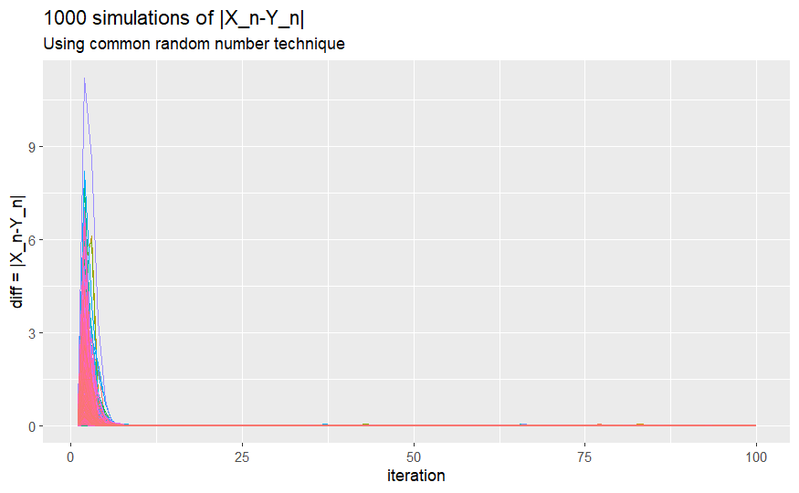
Figure 9: 1000 simulations of $|X_{n,k}-Y_{n,k}|$ where $n=$iteration.

At iteration 35, $E[|\sigma_{35}^{2}-\sigma_{\infty}^{2}|]\leq C\frac{1}{1000}\sum_{i=1}^{1000}|\sigma^{2}_{35,i}-\sigma^{{}^{\prime}2}_{35,i}|=11.4055\times 0.00128\approx 0.0146$. Figure 10 graphs the histogram of $|X_{35,i}-Y_{35,i}|$.

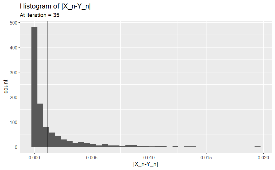
Figure 10: The following histogram graphs $1000$ simulations of $|x_{35,i}-y_{35,i}|$. The vertical line and sample mean difference is $\frac{1}{1000}\sum_{k=1}^{1000}|x_{35,i}-y_{35,i}|=0.0012$

Further, by Lemma 5.2 the total variation distance is bounded above by $\frac{n+\upsilon_{0}}{\upsilon_{0}c_{0}^{2}}=3.5$ times the expected distance,

$$||\mathcal{L}(\sigma^{2}_{n})-\mathcal{L}(\sigma^{{}^{\prime}2}_{\infty})||_{TV} \leq 3.5E[|\sigma^{2}_{n}-\sigma^{2}_{\infty}|]$$

So at the 35th iteration, $||\mathcal{L}(\sigma^{2}_{n})-\mathcal{L}(\sigma^{{}^{\prime}2}_{\infty})||_{TV}\leq 0.052$.

6 Proof of Theorem 3.3

Proof of Theorem 3.3.

Fix $x,y$ and denote $g(U)=f(F^{-1}_{\theta}(U),x)$ and $h(V)=f(F^{-1}_{\theta}(V),y)$. We write $J(U,V)$ to be the set of joint distributions such that $\mathcal{L}(U)=Unif(0,1),\mathcal{L}(V)=Unif(0,1)$. Finally, note that since $\theta=F^{-1}(U)$ where $F$ is invertible, we interchangeably write the set $A$ to signify $A$ (defined on $\theta$) and $F(A)$ (defined on $U,V$).

Also note that since $g(U),h(V)$ are assumed to be of bounded variation, the sets $I_{x},I_{y},D_{x},D_{y}$ can be written as the union of countable intervals by corollary 3.6 of [44].

First we show that

$$\sup_{J(U,V)}E[g(U)h(V)1_{A}]=E[g(U)h(U)1_{A}]$$ (19)

Denote $I_{x}\cap I_{y}=\cup_{k\geq 1}J_{k}$ and $A\setminus(I_{x}\cap I_{y})=\cup_{k\geq 1}L_{k}$ where $J$ and $L$ are intervals.

$$\sup_{J(U,V)}E[g(U)h(V)1_{A}] \leq\sup_{J(U,V)}E[g(U)h(V)1_{I_{x}\cap I_{y}}]+\sup_{J(U,V)}E[g(U)h(V)1_{A\setminus(I_{x}\cap I_{y})}]$$

$$=\sup_{J(U,V)}E[g(U)h(V)1_{I_{x}\cap I_{y}}]+\sup_{J(U,V)}E[(-g(U))(-h(V))1_{A\setminus(I_{x}\cap I_{y})}]$$

$$=\sup_{J(U,V)}E[\sum_{k\geq 1}g(U)h(V)1_{J_{k}}]+\sup_{J(U,V)}E[\sum_{k\geq 1}(-g(U))(-h(V))1_{L_{k}}]$$

$$=\sup_{J(U,V)}\sum_{k\geq 1}E[g(U)h(V)1_{J_{k}}]+\sup_{J(U,V)}\sum_{k\geq 1}E[(-g(U))(-h(V))1_{L_{k}}]$$

$$\leq\sum_{k\geq 1}\sup_{J(U,V)}E[g(U)h(V)1_{J_{k}}]+\sum_{k\geq 1}\sup_{J(U,V)}E[(-g(U))(-h(V))1_{L_{k}}]$$

$$=\sum_{k\geq 1}E[g(U)h(U)1_{J_{k}}]+\sum_{k\geq 1}E[(-g(U))(-h(U))1_{L_{k}}]$$

$$=E[g(U)h(U)1_{I_{x}\cap I_{y}}]+E[(-g(U))(-h(U))1_{A\setminus(I_{x}\cap I_{y})}]$$

$$=E[g(U)h(U)1_{A}]$$

The third equality is by the Dominated Convergence Theorem, Theorem 1.5.8 of [14], and the second last equality is by Proposition 3.2.

Since $E[g(U)h(U)]\leq\sup_{J(U,V)}E[g(U)h(V)]\leq E[g(U)h(U)]$, equality follows. Note that Proposition 3.2 can still be applied even if $g(U)h(U)1_{J_{k}}$ and $g(U)h(U)1_{L_{k}}$ are no longer the product of right continuous functions, which is a result of the fact that $1_{J_{k}}$ may not necessarily be right continuous. This is because the theorem still applies by discussions in Section 4 of [7] that note that rather than requiring that $f(\theta,x)$ be right continuous it is simply necessary to assume that the discontinuous points are countable and have left and right limits. This is a necessary condition for bounded variation (assumed in theorem). Since the function $I_{A}$ has countably many discontinuities, Proposition 3.2 can be used.

Second we show that

$$\sup_{J(U,V)}E[g(U)h(V)1_{A^{c}}]=E[g(U)h(1-U)1_{A^{c}}]$$ (20)

Suppose $A^{c}$ can also be written as countable intervals. The set $A^{c}$ represents areas where either $g$ is increasing and $h$ is decreasing or vice versa. By similar reasoning to equation 19,

$$\sup_{J(U,V)}E[g(U)h(V)1_{A^{c}}] =-\inf_{J(U,V)}E[g(U)(-h(V))1_{A^{c}}]$$

$$=-\inf_{J(U,V)}E[\sum_{I\in A^{c}}g(U)(-h(1-U))I]$$

$$=-\inf_{J(U,V)}\sum_{I\in A^{c}}E[g(U)(-h(1-U))I]$$

$$\leq-\sum_{I\in A^{c}}\inf_{J(U,V)}E[g(U)(-h(1-U))I]$$

$$=-\sum_{I\in A^{c}}E[g(U)(-h(1-U))I]$$

$$=-E[g(U)(-h(1-U))1_{A^{c}}]$$

$$=E[g(U)h(1-U)1_{A^{c}}]$$

The third equality is by the Dominated Convergence Theorem, Theorem 1.5.8 of [14], and the third last equality is by Theorem 2 of [7].

Again, since $E[g(U)h(1-U)1_{A^{c}}]\leq\sup_{J(U,V)}E[g(U)h(V)1_{A^{c}}]\leq E[g(U)h(1-U)1_{A^{c}}]$, equality follows.

Case 1: Suppose $P(A)=1$. We write $P(A^{c})=P(U,V)\in F(A^{c}))$

$$\sup_{J(U,V)}E[g(U)h(V)]$$

$$=\sup_{J(U,V)}E[g(U)h(V)1_{A}]+E[g(U)h(V)1_{A^{c}}]$$

$$=\sup_{J(U,V)}E[g(U)h(V)1_{A}]+E[g(U)h(V)\mid(U,V)\in F(A^{c})]P(A^{c})$$

$$=\sup_{J(U,V)}E[g(U)h(V)1_{A}] P(A^{c})=0$$ Since

$$=E[g(U)h(U)1_{A}]$$ by equation 19

$$=E[g(U)h(U)]$$

By equation 4, equation 8 follows.

Case 2: Suppose $P(A)=0$.

$$\sup_{J(U,V)}E[g(U)h(V)]$$

$$=E[g(U)h(1-U)1_{A^{c}}]$$ by equation 20

$$=E[g(U)h(1-U)]$$

By equation 4, equation 9 follows.

Case 3: Suppose $0<P(A)<1$.

$$\sup_{J(U,V)}E[g(U)h(V)]$$

$$\leq\sup_{J(U,V)}E[g(U)h(V)1_{A}]+\sup_{J(U,V)}E[g(U)h(V)1_{A^{c}}]$$

$$=E[g(U)h(U)1_{A}]+E[g(U)h(1-U)1_{A^{c}}]$$ by equations 19 and 20

By equation 4, equation 10 follows. ∎

References

- [1] David Aldous and Persi Diaconis “Strong uniform times and finite random walks” In Advances in Applied Mathematics 8.1, 1987, pp. 69–97 DOI: 10.1016/0196-8858(87)90006-6
- [2] Niloy Biswas and Lester Mackey “Bounding Wasserstein distance with couplings”, 2021 DOI: arXiv:2112.03152
- [3] Niloy Biswas, Anirban Bhattacharya, Pierre E. Jacob and James E. Johndrow “Coupling-based Convergence Assessment of some Gibbs Samplers for High-Dimensional Bayesian Regression with Shrinkage Priors” In Journal of the Royal Statistical Society Series B: Statistical Methodology 84.3, 2022, pp. 973–996 DOI: 10.1111/rssb.12495
- [4] Simon Breneis “Functions of bounded variation in one and multiple dimensions”, 2020
- [5] “Handbook of Markov chain Monte Carlo” Chapman & Hall, 2011
- [6] Brian S. Caffo, James G. Booth and A.. Davison “Empirical Supremum Rejection Sampling” In Biometrika 89.4 Oxford University Press, Biometrika Trust, 2002, pp. 745–754 DOI: 10.1093/biomet/89.4.745
- [7] Stamatis Cambanis, Gordon Simons and William Stout “Inequalities for Ek(X, Y) when the marginals are fixed” In Zeitschrift für Wahrscheinlichkeitstheorie und Verwandte Gebiete 36.4, 1976, pp. 285–294 DOI: 10.1007/BF00532695
- [8] Pietro Caputo, Cyril Labbé and Hubert Lacoin “Mixing time of the adjacent walk on the simplex” In The Annals of Probability 48.5 Institute of Mathematical Statistics, 2020, pp. 2449–2493 DOI: 10.1214/20-AOP1428
- [9] Mary Katherine Cowles and Jeffrey S. Rosenthal “A simulation approach to convergence rates for Markov chain Monte Carlo algorithms” In Statistics and Computing 8 Institute of Mathematical StatisticsBernoulli Society, 1998, pp. 115–124 DOI: 10.1023/A:1008982016666
- [10] Mary Kathryn Cowles and Bradley P. Carlin “Markov Chain Monte Carlo Convergence Diagnostics: A Comparative Review” In Journal of the American Statistical Association 91, 1996, pp. 883–904 DOI: 10.2307/2291683
- [11] Liyi Dai “Convergence rates of finite difference stochastic approximation algorithms part II: implementation via common random numbers” In Sensing and Analysis Technologies for Biomedical and Cognitive Applications 9871 SPIE, 2016 DOI: 10.1117/12.2228251
- [12] Persi Diaconis and David Freedman “Iterated random functions” In SIAM Review 41.1, 1999, pp. 45–76 DOI: 10.1137/S0036144598338446
- [13] Annette J. Dobson and Adrian G. Barnett “An Introduction to Generalized Linear Models” New York: Texts in Statistical Science. ChapmanHall, 2008 DOI: 10.1201/9780367807849
- [14] Rick Durrett “Probability: Theory and Examples” New York: Cambridge Series in StatisticalProbabilistic Mathematics, 2010 DOI: 10.5555/1869916
- [15] Charles J. Geyer “Introduction to Markov Chain Monte Carlo” In Handbook of Markov Chain Monte Carlo New York: ChapmanHall/CRC, 2011, pp. 1–46 DOI: 10.1201/b10905
- [16] Ramen Ghosh and Jakub Marecek “Iterated Function Systems: A Comprehensive Survey”, 2022 DOI: arXiv.2211.14661
- [17] Alison L. Gibbs “Convergence in the Wasserstein Metric for Markov Chain Monte Carlo Algorithms with Applications to Image Restoration” In Stochastic Models 20.4 Taylor & Francis, 2004, pp. 473–492 DOI: 10.1081/STM-200033117
- [18] Paul Glasserman and David D. Yao “Some guidelines and guarantees for common random numbers” In Management Science 38, 1992, pp. 884–908 DOI: 10.5555/2909967.2909978
- [19] Jeremy Heng and Pierre E. Jacob “Unbiased Hamiltonian Monte Carlo with couplings” In Biometrika 106.2, 2019, pp. 287–302 DOI: 10.1093/biomet/asy074
- [20] James P. Hobert and Galin L. Jones “Honest Exploration of Intractable Probability Distributions via Markov Chain Monte Carlo” In Statistical Science 16.4 Institute of Mathematical Statistics, 2001, pp. 312–334 DOI: 10.1214/ss/1015346317
- [21] Peter D. Hoff “A First Course in Bayesian Statistical Methods” New York: Springer, 2009 DOI: 10.1007/978-0-387-92407-6
- [22] Pierre E. Jacob “Lecture notes for couplings and Monte Carlo”, Available at https://sites.google.com/site/pierrejacob/cmclectures?authuser=0 (2021/09/17)
- [23] S.. Jarner and R.. Tweedie “Locally Contracting Iterated Functions and Stability of Markov Chains” In Journal of Applied Probability 38.2, 2001, pp. 494–507 DOI: 10.1239/jap/996986758
- [24] Zhumengmeng Jin and James P. Hobert “Dimension free convergence rates for Gibbs samplers for Bayesian linear mixed models” In Stochastic Processes and their Applications 148, 2022, pp. 25–67 DOI: 10.1016/j.spa.2022.02.003
- [25] Valen E. Johnson “Studying convergence of Markov Chain Monte Carlo algorithms using coupled sample paths” In Journal of the American Statistical Association 91, 1996, pp. 154–166 DOI: 10.1080/01621459.1996.10476672
- [26] Oliver Jovanovski and Neal Madras “Convergence rates for a hierarchical Gibbs sampler” In Bernoulli 1.23, 2013, pp. 603–625 DOI: 10.3150/15-BEJ758
- [27] Anthony Lee, Sumeetpal S. Singh and Matti Vihola “Coupled conditional backward sampling particle filter” In The Annals of Statistics 48.5 Institute of Mathematical Statistics, 2020, pp. 3066–3089 DOI: 10.1214/19-AOS1922
- [28] Krzysztof Leśniak, Nina Snigireva and Filip Strobin “Weakly contractive iterated function systems and beyond: a manual” In Journal of Difference Equations and Applications 26.8, 2020, pp. 1114–1173 DOI: 10.1080/10236198.2020.1760258
- [29] Neal Madras and Denise Sezer “Quantitative bounds for Markov chain convergence: Wasserstein and total variation distances” In Bernoulli 16.3, 2010, pp. 882–908 DOI: 10.2307/25735016
- [30] Tamás P. Papp and Chris Sherlock “A new and asymptotically optimally contracting coupling for the random walk Metropolis”, 2022 DOI: arXiv:2211.12585
- [31] Natesh S. Pillai and Aaron Smith “Kac’s walk on -sphere mixes in steps” In The Annals of Applied Probability 27.1 Institute of Mathematical Statistics, 2017, pp. 631–650 DOI: 10.1214/16-AAP1214
- [32] Alexander S. Poznyak “Advanced Mathematical Tools for Automatic Control Engineers: Deterministic Techniques” Oxford: Elsevier, 2008 DOI: 10.1016/B978-008044674-5.50001-8
- [33] James Gary Propp and David Wilson “Coupling from the past: A user’s guide” In Microsurveys in Discrete Probability, 1997 DOI: 10.1090/dimacs/041/09
- [34] Qian Qin and James P. Hobert “Geometric convergence bounds for Markov chains in Wasserstein distance based on generalized drift and contraction conditions” In Annales de l’Institut Henri Poincaré, Probabilités et Statistiques 58.2 Institut Henri Poincaré, 2022, pp. 872–889 DOI: 10.1214/21-AIHP1195
- [35] Qian Qin and James P. Hobert “Wasserstein-based methods for convergence complexity analysis of MCMC with applications” In The Annals of Applied Probability 32.1 Institute of Mathematical Statistics, 2022, pp. 124–166 DOI: 10.1214/21-AAP1673
- [36] Svetlozar T. Rachev, John S.. Hsu, Biliana S. Bagasheva and Frank J. Fabozzi “Bayesian Methods in Finance” New York: WileySons, 2008 DOI: 10.1002/9781119202141
- [37] Gareth O. Roberts and Jeffrey S. Rosenthal “General state space Markov chains and MCMC algorithms” In Probability surveys 1 Institute of Mathematical StatisticsBernoulli Society, 2004, pp. 20–71
- [38] Gareth O. Roberts and Jeffrey S. Rosenthal “One-shot coupling for certain stochastic recursive sequences” In Stochastic Processes and their Applications 99, 2002, pp. 195–208 DOI: 10.1016/S0304-4149(02)00096-0
- [39] Sheldon M. Ross “Introduction to Probability Models” Academic Press, 2010
- [40] Vivekananda Roy “Convergence Diagnostics for Markov Chain Monte Carlo” In Annual Review of Statistics and Its Application 7.1, 2020, pp. 387–412 DOI: 10.1146/annurev-statistics-031219-041300
- [41] H.. Roydon “Real Analysis” Macmillian, 1968
- [42] Filippo Santambrogio “Optimal Transport for Applied Mathematicians. Calculus of Variations, PDEs and Modeling” Birkauser, 2015 DOI: 10.1007/978-3-319-20828-2
- [43] Sabrina Sixta and Jeffrey S. Rosenthal “Convergence rate bounds for iterative random functions using one-shot coupling” In Statistics and Computing 32.71, 2022, pp. 1573–1375 DOI: 10.1007/s11222-022-10134-x
- [44] Elias M Stein and Rami Shakarchi “Real analysis: measure theory, integration, and Hilbert spaces”, Princeton lectures in analysis Princeton, NJ: Princeton Univ. Press, 2005 DOI: 10.2307/j.ctvd58v18
- [45] David Steinsaltz “Locally Contractive Iterated Function Systems” In Annals of Probability 27.4, 1999, pp. 1952–1979 DOI: 10.1214/aop/1022874823
- [46] Örjan Stenflo “A Survey of Average Contractive Iterated Function Systems” In Journal of Difference Equations and Applications 18.8, 2012, pp. 1355–1380 DOI: 10.1080/10236198.2011.610793
- [47] Luke Tierney “Markov chains for exploring posterior distributions” In Annals of Statistics 22, 1994, pp. 1701–1728
- [48] Guanyang Wang, John O’Leary and Pierre E. Jacob “Maximal Couplings of the Metropolis-Hastings Algorithm” In International Conference on Artificial Intelligence and Statistics, 2021, pp. 1225–1233
- [49] Ward Whitt “Bivariate Distributions with Given Marginals” In The Annals of Statistics 4.6 Institute of Mathematical Statistics, 1976, pp. 1280–1289 DOI: 10.1214/aos/1176343660
- [50] James R. Wilson “Antithetic Sampling with Multivariate Inputs” In American Journal of Mathematical and Management Sciences 3.2 Taylor & Francis, 1983, pp. 121–144 DOI: 10.1080/01966324.1983.10737119
- [51] Kai Xu, Tor Erlend Fjelde, Charles Sutton and Hong Ge “Couplings for Multinomial Hamiltonian Monte Carlo” In Proceedings of The 24th International Conference on Artificial Intelligence and Statistics 130 PMLA, 2021, pp. 3646–3654