Distributed Pilot Assignment for Distributed Massive-MIMO Networks

Abstract

Pilot contamination is a critical issue in distributed massive MIMO networks, where the reuse of pilot sequences due to limited availability of orthogonal pilots for channel estimation leads to performance degradation. In this work, we propose a novel distributed pilot assignment scheme to effectively mitigate the impact of pilot contamination. Our proposed scheme not only reduces latency, but it also enhances fault-tolerance. Extensive numerical simulations are conducted to evaluate the performance of the proposed scheme. Our results establish that the proposed scheme outperforms existing centralized and distributed schemes in terms of mitigating pilot contamination and significantly enhancing network throughput.

I Introduction

The rapid growth and adoption of wireless communication based data services has prompted the development of technologies that can improve the capacity, reliability, and efficiency of cellular networks. By reaping the benefits of mMIMO and Ultra Dense Network (UDN), Distributed mMIMO is emerging as a promising technology [1, 2]. It abandons the concept of distinct cells but instead deploys a large number of distributed access points (APs) throughout the coverage area [1]. As there are no traditional cells, the inter-cell interference that plagues cellular systems is eliminated. Further, as the user equipments (UEs) are very close to APs, this may provide high coverage probability in the network, thus improving quality-of service to the users. However, as in traditional mMIMO systems, channel estimation is a critical challenge in distributed mMIMO networks. One commonly employed approach is blind convolution techniques, such as matrix decomposition-based signal detection. However, these methods often have high computational complexity. To mitigate this complexity, researchers have explored leveraging the channel hardening property of mMIMO systems [3]. However, in distributed mMIMO, the channel hardening is not always guaranteed [4], so getting the estimates using matrix decomposition-based channel estimation is not a viable option.

Pilot-based channel estimation presents a simple and low-complexity approach that can be employed within the distributed mMIMO systems to obtain channel estimates. However, before deploying such solutions in the networks an associated issue of pilot contamination needs to be addressed. Pilot contamination arises when the same pilot sequences are used for estimating channels of more than one user, leading to estimation errors and subsequent performance degradation. In a practical system, as it is almost impossible to assign orthogonal pilots to all users, the users may reuse the pilots. To minimize the impact of pilot contamination, pilot assignment (PA) should be carried out so that it minimizes the contamination. A lot of work on pilot assignment in distributed mMIMO networks exists, but most of it is centralized in nature [1, 5, 6, 7, 8, 9, 10, 11]. In [1], the authors have proposed two pilot assignment schemes namely random pilot assignment and greedy pilot assignment based on throughput improvement. In [5], the authors have proposed a scalable scheme which performs joint pilot assignment and AP-UE association. In [6], the authors have proposed a graph coloring-based pilot assignment, where the AP-UE association takes place initially and then pilots are assigned using graph coloring. If the pilot assignment fails, the AP-UE associations are updated, and so is the pilot assignment. In [7], the authors have proposed a pilot assignment scheme based on Hungarian matching algorithm. In [8], the authors have proposed a clustering based scalable pilot scheme where UEs in the same cluster are allocated the same pilots. In [9], the authors have again exploited the graph theory, but instead by graph coloring, they have used weighted graph approach. In [10], the authors have tried to exploit the interference-aware reward, calculated by treating noise as a interference, for the pilot assignment and AP-UE association jointly. Along with random pilot assignment [1], that can also be implemented in distributed manner, there are a few distributed schemes [12, 13]. In [12], the authors have proposed a survey propagation based distributed pilot assignment scheme that incurs high signaling overhead due to messages passing among the feasible groups. Also, for the proposed scheme the computational cost increases drastically as the number of users-to-pilots ratio increases. In [13], the authors have proposed a distributed multi-agent reinforcement learning-based pilot assignment. This, however, demands centralized training, resulting in increased signaling overhead, sensitivity to the training data, and lack of explainability of the model.

To address these challenges, a distributed pilot assignment scheme for distributed mMIMO systems is proposed in this paper. The novelty of proposed work is rooted in distributed scheme that jointly performs the pilot assignment and AP-UE association. In this scheme orthogonal pilot signals are allocated to the topmost UEs of each AP, determined by the largest large-scale fading coefficient. Subsequently, each AP independently associates itself with these topmost UEs with different pilot signals. The proposed scheme not only reduces latency in distributed mMIMO networks, but also improves the overall spectral efficiency. We compare the performance of the proposed scheme with existing schemes through extensive numerical simulations and establish its superiority in terms of scalability and overall system throughput.

Organization: The paper is structured as follows: Section II presents the system model. Section III introduces the proposed distributed resource allocation scheme. Section IV evaluates performance of the proposed scheme and demonstrates its effectiveness. Finally, Section V concludes the paper by summarizing our work and discussing its future directions.

II System Model

We consider a distributed mMIMO network configuration comprising of T UEs and M APs. The set of UEs is denoted as $\mathcal{T}$, while the set of APs is denoted as $\mathcal{M}$. Each AP is equipped with A antennas, while each UE is equipped with a single antenna. Both the APs and UEs are uniformly distributed over the coverage area. To facilitate the coordination and processing of UE signals, the APs are connected to a Central Processing Unit (CPU) through a front-haul connection. To minimize computation cost and front-haul overload, a scalable architecture is employed [5]. This architecture leverages the observation that more than 95% of the received signal strength is concentrated in a few nearby APs [14]. We consider the TDD mode for our operations and assume channel reciprocity. To model the wireless channel, we consider a standard block fading model with a resource block of length $L_{c}$. The channel coefficient $\textbf{h}_{t,m}\in\mathbb{C^{\textit{A}}}$ represents the spatially correlated Rayleigh fading channel between the $t^{th}$ UE and the $m^{th}$ AP. It follows a complex Gaussian distribution such that $\textbf{h}_{t,m}{\sim}\mathcal{N}_{\mathbb{C}}(0,\textbf{R}_{t,m})$, where $\textbf{R}_{t,m}\in\mathbb{C}^{\textit{A}\times\textit{A}}$ represents the spatially correlated matrix that incorporates large-scale fading coefficient (LSFC), denoted by $\beta_{t,m}$, that accounts for various factors such as path-loss and shadow-fading and can be calculated by utilizing periodically broadcasted synchronization signals from the UE $t$ to the AP $m$, [5]. We assume that these channel vectors of a particular UE for different APs are independent and this assumption is reasonable as APs are distributed over a large area.

Let $L_{p}$ denote the number of mutually orthogonal pilots such that the length $L_{p}$ of each resource block is used for pilot training and the remaining for information transmission. As number of orthogonal pilots is smaller than the number of UEs, so pilot reuse comes into play. Let $\mathcal{T}_{p}$ be the subset of UEs sharing the pilot $p$. Following [5], the received signal $\textbf{y}_{p,m}\in\mathbb{C^{\textit{A}}}$ at the $m^{th}$ AP when the pilot $p$ is transmitted by UEs belonging to $\mathcal{T}_{p}$ is given by :

$$\textbf{y}_{p,m}=\sum_{t\in\mathcal{T}_{p}}\sqrt{L_{p}\tau_{t}}\textbf{h}_{t,m}+\textbf{n}_{m},$$ (1)

where $\tau_{t}$ is the uplink transmit power of the UE $t\in\mathcal{T}_{p}$ and $\textbf{n}_{m}{\sim}\mathcal{N}_{\mathbb{C}}(0,\sigma^{2}\mathbf{I}_{A})$ denotes the noise at the $m^{th}$ AP. The MMSE estimate of channel $\textbf{h}_{t,m}$ is given by

$$\hat{\textbf{h}}_{t,m}=\sqrt{L_{p}\tau_{t}}\textbf{R}_{t,m}\boldsymbol{\Psi}^{-1}_{t,m}\textbf{y}_{p,m},$$ (2)

where $\boldsymbol{\Psi}_{t,m}=\sum_{t{\in}\mathcal{T}_{p}}\sqrt{L_{p}\tau_{t}}\textbf{R}_{t,m}+\sigma^{2}\mathbf{I}_{A}$ is the correlation matrix of $\textbf{y}_{p,m}$. The pilot sharing not only leads to poorer channel estimation, but also affects $\hat{\textbf{h}}_{t,m}$, which becomes more correlated and thus increases the interference among the UEs.

The association of the UE $t$ and the AP $m$ is denoted by a indicator variable $d_{t,m}$, which equals ’$1$’ when the UE $t$ is served by the AP $m$, and ’$0$’ when the UE $t$ is not so served. The received uplink signal at the AP $m$ is given by

$$\textbf{y}^{u}_{m}=\sum\limits_{t=1}^{T}\tau_{t}\textbf{h}_{t,m}d_{t,m}x_{t}+\textbf{n}_{m}.$$ (3)

The payload signal $x_{t}\in\mathbb{C}$ is the unit power complex signal sent by the UE $t$ and the power associated with it is denoted by $\tau_{t}$. The combining vector $\textbf{v}_{t,m}\in\mathbb{C}^{\textit{A}}$ is assigned to the UE $t$ by the AP $m$. The estimate of ${x}_{t}$ is $\hat{x}_{t}=\sum_{t{\in}T}d_{t,m}\textbf{v}^{H}_{t,m}\textbf{y}^{u}_{m}$.

The uplink spectral efficiency (SE) is [5]

$$\mathsf{SE}^{u}_{t}=(1-\frac{L_{p}}{L_{c}})\mathbb{E}\{\log_{2}(1+\mathsf{SINR}^{u}_{t})\},$$ (4)

where $\mathsf{SINR}^{u}_{t}$ represents the uplink instantaneous signal to noise plus interference ratio of the $t^{th}$ UE and is given by [5]

$$\mathsf{SINR}^{u}_{t}=\frac{\tau_{t}|\sum\limits^{M}_{m=1}d_{t,m}\textbf{v}^{H}_{t,m}\hat{\textbf{h}}_{t,m}|^{2}}{\sum\limits^{T}_{j=1,j\neq t}\tau_{j}|\sum\limits^{M}_{m=1}d_{t,m}\textbf{v}^{H}_{t,m}\hat{\textbf{h}}_{t,m}|^{2}+\textbf{z}_{t}},$$ (5)

where $\textbf{z}_{t}=\sum^{M}_{m=1}d_{t,m}\textbf{v}^{H}_{t,m}(\sum^{T}_{t=1}\tau_{t}\textbf{C}_{t}+\sigma^{2}\mathbf{I}_{MA})\textbf{v}_{t,m}$, and $\textbf{C}_{t}$ is the error correlation matrix for the collective channel of the UE $t$.

The precoding vector, $\textbf{s}_{t,m}{\in}\mathbb{C}^{A}$, assigned to the $t^{th}$ UE by the $m^{th}$ AP and the received downlink signal at the $t^{th}$ UE respectively, are:

$$\textbf{s}_{t,m}=\sqrt{\tau_{t,m}}\frac{\hat{\textbf{h}}_{t,m}}{\sqrt{\mathbb{E}||\hat{\textbf{h}}_{t,m}||^{2}}},$$ (6)

$${y}^{d}_{t}=\sum\limits_{m=1}^{M}\textbf{h}^{H}_{t,m}\sum\limits_{j=1}^{T}d_{j,m}\textbf{s}_{j,m}x_{j}+n_{t},$$ (7)

where $n_{t}{\sim}\mathcal{N}_{\mathbb{C}}(0,\sigma^{2})$ is the thermal noise, $x_{j}\in\mathbb{C}$ is unit power complex signal sent to the $t^{th}$ UE and $\tau_{t,m}$ is the downlink power assigned to the $t^{th}$ UE by the $m^{th}$ AP, allocated using the fraction power allocation [5].

By utilizing the use-and-then-forget bound [15], the downlink spectral efficiency (SE) is

$$\mathsf{SE}^{d}_{t}=(1-\frac{L_{p}}{L_{c}})\log_{2}(1+\mathsf{SINR}^{d}_{t}),$$ (8)

where $\mathsf{SINR}^{d}_{t}$ represents the downlink instantaneous signal to noise plus interference ratio of the $t^{th}$ UE and is given by

$$\mathsf{SINR}^{d}_{t}=\frac{|\mathbb{E}\{{\sum\limits^{M}_{m=1}d_{t,m}\textbf{h}^{H}_{t,m}\textbf{s}_{t,m}}\}|^{2}}{\textbf{z}-|\mathbb{E}\{{\sum\limits^{M}_{m=1}d_{t,m}\textbf{h}^{H}_{t,m}\textbf{s}_{t,m}}\}|^{2}+\sigma^{2}},$$ (9)

where $\textbf{z}=\sum^{T}_{j=1}|\mathbb{E}\{{\sum^{M}_{m=1}d_{j,m}\textbf{h}^{H}_{j,m}\textbf{s}_{j,m}}\}|^{2}$.

III Distributed Pilot Allocation

We propose a distributed pilot assignment scheme to address the limitations on the number of mutually orthogonal pilots ($L_{p}{<}T$) and mitigate pilot contamination. A key prerequisite for distributed mMIMO is that each UE be served by at least one AP. Additionally, each AP must assign a given pilot to at most one UE to minimize pilot contamination. To guarantee that each UE is served by at least one AP and to manage pilot assignment, a specific AP is designated as the controller-AP for each UE. Therefore, in the proposed scheme first, a controller-AP is assigned to each UE in a distributed manner. Then, pilots are assigned distributively to each UE by its associated controller-AP. Furthermore, to fully leverage the benefits of mMIMO and make the system scalable, each UE needs to be connected to an adequate number of APs. To achieve this, a distributed AP-UE clustering scheme is employed in the final step based on the constraint that each AP serves one UE per pilot, thus minimizing pilot contamination while providing significant power to the UEs.

For each AP $m$, we define a subset $\mathcal{U}_{m}$ of UEs that includes, at most, the leading $L_{p}$ UEs of the $m^{th}$ AP, as determined by the decreasing order of the parameter $\beta_{t,m}$. Let $\mathcal{T}_{m}^{c}$ be the subset of UEs with the AP $m$ as their controller-AP. We define $\mathcal{L}_{t}^{p}$ as the set of available pilots for UE $t$, initially contains all $L_{p}$ pilots.

III-A Controller-AP assignment

For the controller-AP assignment, we propose a distributed algorithm. In the proposed approach, each UE is responsible for selecting its controller-AP from the set of available APs using their respective LSFC values, by following the standard random access procedure [16] with the broadcast signal [5]. However, there is a challenge when more than $L_{p}$ UEs intend to be allocated a particular AP as their controller-AP. This challenges our design requirement that each AP can serve at most one UE per pilot. However, another issue is that, if a UE requests an AP with a lower LSFC value to be its controller-AP, this could potentially lead to degradation in the system performance. To address these, we propose a Controller-AP selection algorithm, where each UE is assigned one AP from the set $\mathcal{M}_{t}^{c}$ of APs as its controller-AP. Also, an AP can serve as the controller-AP of at most $L_{p}$ UEs. The details of constructing subset $\mathcal{M}_{t}^{c}$ are given in Algorithm 1. In order to identify the APs that are serving more than $L_{p}$ UEs and require some of their associated UEs to request a new controller-AP assignment, and the APs that are just serving $L_{p}$ UEs and so are unable to accept controller-AP requests for more UEs, the APs are categorized into two set. The former are called the oversaturated-APs and are denoted as $\mathcal{M}_{D}$, and the latter are called the inert-APs and are denoted as $\mathcal{M}_{I}$, respectively. The detailed procedure to select controller-AP distributively from the set of potential controller-APs is given by Algorithm 1. The Algorithm 1 is carried out at the APs in cooperation with the UEs.

1:  Input: $\mathcal{M}_{t}^{c}=\emptyset$, $\beta_{t,m}$, $\mathcal{T}_{m}^{c}=\emptyset$, $\mathcal{M}_{D}=\emptyset$ and $\mathcal{M}_{I}=\emptyset$ $\forall$ $t{\in}\mathcal{T}$, $m{\in}\mathcal{M}$

2:  Returns: Controller-AP assignment for each UE.

3:  for each UE $t\in\mathcal{T}$ do

4:     Calculate $\beta^{d}_{t}$ as the difference between the largest and second largest LSFC values of $\beta_{t,m}$.

5:  end for

6:  Calculate $\gamma^{th}=((\beta^{d}_{t})_{max}+(\beta^{d}_{t})_{min})/2$.

7:  for each UE $t\in\mathcal{T}$ do

8:     $\mathcal{M}_{t}^{c}=\mathcal{M}_{t}^{c}\cup m_{max},$ where$\ \underset{m}{m_{max}=\operatornamewithlimits{argmax}~{}}\beta_{m,t}$.

9:     for each AP $m\in\mathcal{M}$ do

10:        if  $\beta_{m_{max},t}-\beta_{m,t}<=\gamma^{th}$ then

11:           $\mathcal{M}_{t}^{c}=\mathcal{M}_{t}^{c}\cup m$.

12:        end if

13:     end for

14:     Choose a controller-AP randomly from $\mathcal{M}_{t}^{c}$.

15:  end for

16:  for all  AP $m\in\mathcal{M}$ do

17:     ​​​​​​ Update $\mathcal{T}_{m}^{c}=\mathcal{T}_{m}^{c}\cup t$, where AP m is a controller-AP of UE $t$.

18:     if  $|\mathcal{T}_{m}^{c}|>L_{p}$  then

19:        Update $\mathcal{M}_{D}=\mathcal{M}_{D}\cup m$.

20:     else if $|\mathcal{T}_{m}^{c}|=L_{p}$ then

21:        Update $\mathcal{M}_{I}=\mathcal{M}_{I}\cup m$.

22:     end if

23:  end for

24:  while $\mathcal{M}_{D}\neq\emptyset$ do

25:     for each AP $m{\in}\mathcal{M}_{D}$ do

26:        Arrange $t\in\mathcal{T}_{m}^{c}$ in increasing order of $|\mathcal{M}_{t}^{c}|$, where priority is given to a UE with a larger LSFC w.r.t AP $m$ to form a new set $\mathcal{T}_{new}$.

27:        Set $\mathcal{T}_{m}^{c}=\emptyset$ and include first $L_{p}$ UEs from $\mathcal{T}_{new}$ in $\mathcal{T}_{m}^{c}$.

28:        AP $m$ unassigns itself as the controller-APs of all UEs in $(\mathcal{T}_{new}-\mathcal{T}_{m}^{c})$.

29:        for  each UE $t{\in}(\mathcal{T}_{new}-\mathcal{T}_{m}^{c})$ do

30:           Update $\mathcal{M}_{t}^{c}\leftarrow\mathcal{M}_{t}^{c}-\mathcal{M}_{I}-m$.

31:           Choose a controller-AP randomly from $\mathcal{M}_{t}^{c}$.

32:        end for

33:     end for

34:     Set $\mathcal{M}_{D}=\emptyset$, $\mathcal{M}_{I}=\emptyset$, $\mathcal{T}_{m}^{c}=\emptyset$ and repeat steps in lines 16-23.

35:  end while

Algorithm 1 Controller-AP selection

III-B Distributed Pilot assignment

Now we propose a distributed pilot assignment scheme. In order to minimize pilot contamination, we introduce a contamination matrix Ad, a binary indicator matrix, indicating whether any two UEs can share a pilot or not. Every AP assigns distinct pilots to its serving UEs and informs its neighboring APs in $\mathcal{M}_{m}^{nb}$ about its pilot assignment. The construction of $\mathcal{M}_{m}^{nb}$ is explained in Algorithm 2. If any two UEs have the same pilot and Ad indicates that these two UEs cannot share the pilot, then the AP allows a UE to retain the pilot if either the cardinality of set $\mathcal{L}^{p}_{t}$ for this UE is smaller or its index is smaller than the other UE. The detailed procedure for assigning pilots to UEs is outlined in Algorithm 2. The Algorithm 2 is carried out at the APs.

1:  Input:$\mathcal{M}_{m}^{nb}=\emptyset$, the set of neighboring APs, $\mathcal{T}_{m}^{c}$, $\mathcal{L}^{p}_{t}$, $\mathcal{U}_{m}$, $count=0$, $max\_iter$ and $a_{i,j}=0,\forall i,j,t{\in}\mathcal{T}$ and $m\in\mathcal{M}$.

2:  Returns: Pilot assignment for each UE.

3:  for each AP $m\in\mathcal{M}$ do

4:     for $t\in\mathcal{U}_{m}$ do

5:        if $t\in\mathcal{U}_{m}-\mathcal{T}_{m}^{c}$ then

6:           Update $\mathcal{M}_{m}^{nb}=\mathcal{M}_{m}^{nb}\cup m^{c}_{t}$, where $m^{c}_{t}$ represents the controller-AP of UE $t$.

7:           Update $\mathcal{M}_{m^{c}_{t}}^{nb}=\mathcal{M}_{m}^{nb}\cup m$.

8:        end if

9:     end for

10:     For UEs $t,t^{\prime}{\in}\mathcal{U}_{m},where\ t\neq t^{\prime}$, then $\textbf{Ad}\{t,t^{\prime}\}=1$.

11:  end for

12:  while  any UE $t\in\mathcal{T}$ is not assigned a pilot and $\mathcal{L}_{t}^{p}\neq\emptyset$ do

13:     for  each AP $m$ do

14:        for  each unassigned UE $t\in\mathcal{T}_{m}^{c}$ do

15:           AP $m$ assigns distinct but unused pilots from $\mathcal{L}_{t}^{p}$.

16:        end for

17:     end for

18:     Each AP $m\in\mathcal{M}$ informs the other APs in $\mathcal{M}_{m}^{nb}$ about the pilots of UEs in $\mathcal{T}_{m}^{c}$.

19:     for each AP $m\in\mathcal{M}$ do

20:        for $t\in\mathcal{U}_{m}$ do

21:           for $t^{\prime}\in\mathcal{U}_{m}$ do

22:              if $t$ and $t^{\prime}$ have the same pilot then

23:                 if $|\mathcal{L}_{t}^{p}|>|\mathcal{L}_{t^{\prime}}^{p}|$ then

24:                    The UE $t^{\prime}$ is allowed to keep its pilot.

25:                 else if $|\mathcal{L}_{t}^{p}|=|\mathcal{L}_{t^{\prime}}^{p}|$ then

26:                    The UE with lower index between $t$ and $t^{\prime}$ is allowed to keep its pilot.

27:                 end if

28:              end if

29:           end for

30:        end for

31:     end for

32:     Each AP $m\in\mathcal{M}$ again informs the other APs in $\mathcal{M}_{m}^{nb}$ about the pilots of UEs in $\mathcal{T}_{m}^{c}$.

33:     for  each AP $m$ do

34:        for each UE $t\in\mathcal{T}_{m}^{c}$ do

35:           Updates the $\mathcal{L}_{t}^{p}$ by removing the pilot of UE $t^{\prime}$ for which $\mathbf{Ad}\{t^{\prime},t\}=1,\ \forall t^{\prime}\in\mathcal{T}$.

36:        end for

37:     end for

38:  end while

39:  if  any UE $t$ left unassigned then

40:     The AP $m^{c}_{t}$ assigns an unused pilot to the UE $t$.

41:  end if

Algorithm 2 Distributed Pilot Assignment

III-C UE-AP Clustering

The distributed UE-AP clustering is performed to improve the spectral diversity, as in [5]. Each AP serves at most one UE per pilot in order to minimize the pilot contamination. Initially, each AP $m$ chooses to serve each UE $t\in\mathcal{T}_{m}^{c}$. Then the AP $m$, for each pilot (except pilots of UEs in $\mathcal{T}_{m}^{c}$), chooses a UE to serve based on the largest LSFC.

III-D Complexity analysis

The complexity of graph-coloring based pilot assignment algorithm in [6] is $\mathcal{O}(\textit{T}\textit{M}log_{2}\textit{M}+2\textit{T}\textit{M}+\textit{T}^{2})$. The complexity of scalable PA in [5] is $\mathcal{O}(\textit{T}\textit{M}+\textit{T}\textit{L}_{p}+\textit{M}\textit{L}_{p})$. The complexity of IAR-based PA in [10] is $\mathcal{O}(\textit{T}^{2}\textit{M}+\textit{M}\textit{L}^{3}_{p}+\textit{T}\textit{M}^{2})$.

The complexity of our proposed Algorithm 1 mainly depends upon the execution in lines 24-35, the while loop iterates at most M times, given that any AP can be a unsaturated AP at most once, therefore its worst-case complexity is $\mathcal{O}(\textit{T}\textit{M}^{2})$. The complexity of Algorithm 2 depends on finding the set $\mathcal{M}_{m}^{nb}$ for each AP. This has complexity of $\mathcal{O}(\textit{M}\textit{L}_{p})$. The Algorithm 2 also depends on execution of the while loop between lines 17-36. Assuming the while loop runs $I$ times, the complexity of execution of the while loop is $\mathcal{O}(\textit{I}\textit{M}\textit{L}^{2}_{p})$. Therefore, the overall complexity of Algorithm 2 is $\mathcal{O}(\textit{M}L_{p}+\textit{I}\textit{M}\textit{L}^{2}_{p})$. The final complexity of overall procedure including AP-UE association is $\mathcal{O}(\textit{T}\textit{M}^{2}+\textit{M}\textit{L}_{p}+\textit{I}\textit{M}\textit{L}^{2}_{p}+\textit{M}\textit{L}_{p})$. Putting everything together, the overall complexity of our proposed scheme is $\mathcal{O}(\textit{T}\textit{M}^{2}+\textit{I}\textit{M}\textit{L}^{2}_{p})$. The actual execution time of the aforementioned processes may be substantially lower when compared to the complexities given above, primarily due to opportunities for extensive parallel execution of various processes within the procedure. In Algorithm 1, the formation of the sets $\mathcal{M}_{D}$ and $\mathcal{M}_{I}$ may take place at the APs independently. Similarly, each AP in $\mathcal{M}_{D}$ may run the while loop in Algorithm 1 in parallel. This may further reduce the execution time significantly. In Algorithm 2, the pilot assignment is being carried out in parallel at the APs, thus reducing the execution time.

IV Performance Evaluation

For numerical simulations we have considered an area of $2000\times 2000$ square meters in which T UEs and 100 APs are uniformly distributed. Each AP is equipped with 4 antennas. We have considered APs to be 10 meters higher than the UEs. We set $L_{c}=200,\ L_{p}=10,\ \tau_{t}=100\ mW$ and $1000\ mW$ downlink power of each AP. We have considered bandwidth to be 20 MHz. To simulate the large scale propagation model, we have considered the 3GPP Urban Microcell scenario and the local scattering model for spatial correlation same as in [17]. We have averaged our results over 50 network instances and for each instance we have considered 500 channel realizations. For all the simulations, P-MMSE precoder [5] is used. For spectral efficiency comparison we have considered centralized schemes, such as scalable PA [5], IAR-sum PA [10], graph-coloring-based PA [6]; and a distributed scheme: survey-propagation-based (survey) PA [12]. For a fair comparison, in scalable and survey-propagation, a AP can serve at most $L_{p}$ UEs.

IV-A Downlink Operations

IV-A1 Comparison with centralized schemes

Fig. 1 shows the plot of the 90%-likely downlink SE for different numbers of UEs. The proposed distributed scheme outperforms the scalable PA scheme by 2%, the graph-coloring PA scheme by 2%, and the IAR-sum PA scheme by 6% in scenario involving 100 UEs. Similarly, improvements with 150 UEs are 3%, 18%, and 9% respectively, and improvements with 200 UEs are 7%, 36%, and 7%, respectively. It can also be observed that as the number of UEs increases, the 90%-likely downlink SE of all schemes decreases, but our proposed scheme sees a lesser decrease than all other schemes. These results demonstrates the superiority of our proposed scheme in terms of 90%-likely downlink SE than all other schemes for all user scenarios.

Figure 1: 90%-likely downlink SE vs $T$.

Similarly Fig. 2 shows the graph between average downlink SE for different numbers of UEs. For $T=100$, our proposed scheme demonstrates superior performance compared to the graph-coloring PA and IAR-sum PA by 22% and 1% respectively. However, it is slightly outperformed (by 1%) by the scalable PA. For $T=150$, the proposed scheme outperforms both the graph-coloring based PA and the IAR-sum PA, while achieving comparable performance to the scalable PA. Finally, for $T=200$, the proposed scheme surpasses all other schemes.

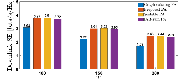
Figure 2: Average downlink SE vs $T$.

IV-A2 Comparison with a distributed scheme

Fig. 3 shows the CDF of 90%-likely downlink SE for distributed PA schemes. To decrease the computational cost of the distributed survey PA scheme, we have considered the number of UEs to the number of pilots ratio to be $3$. The plot shows that the proposed scheme outperforms the survey-propagation-based scheme, thus demonstrating its superiority.

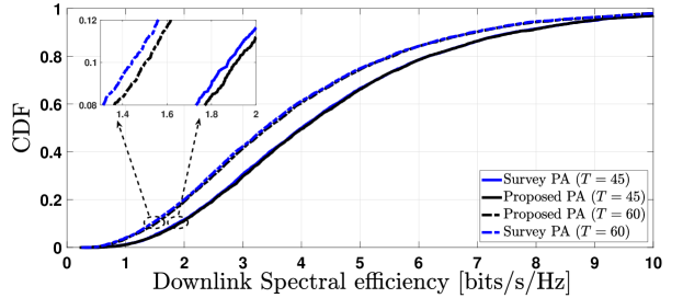
Figure 3: CDF of downlink SE, when $\frac{T}{L_{p}}=3$.

IV-B Uplink Operations

IV-B1 Comparison with centralized schemes

Fig. 4 shows the plot of the 90%-likely uplink spectral efficiency for different numbers of UEs. In a scenario involving 100 UEs, the proposed approach outperforms the scalable PA technique by 1%, the graph-coloring-based PA scheme by 36%, and the IAR-sum PA scheme by 4%. Similarly, with 150 UEs, improvements are 3%, 72%, and 6%, respectively, and improvements with 200 UEs are 11%, 105%, and 9%, respectively. It can also be seen that when the number of UE increases, the 90%-likely downlink SE of all schemes decreases, however our proposed scheme has a lesser decrease than all other schemes.

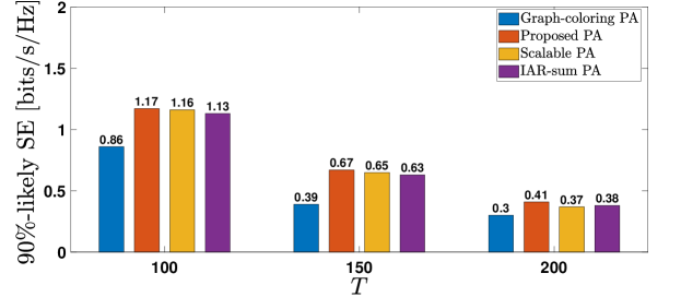
Figure 4: 90%-likely uplink SE vs $T$.

Fig. 5 shows the graph between average uplink SE for different numbers of UEs. For $T=100$, our proposed scheme demonstrates superior performance compared to the graph-coloring PA by approximately 17% and the IAR-sum PA by nearly 2%. It is, however, outperformed (by $\leq$ 1%) by the scalable PA. The proposed scheme surpasses both the graph-coloring-based PA and the IAR-sum PA by a significant margin for $T=150$, while matching the scalable PA performance. Finally, for $T=200$, our proposed scheme surpasses all other schemes.

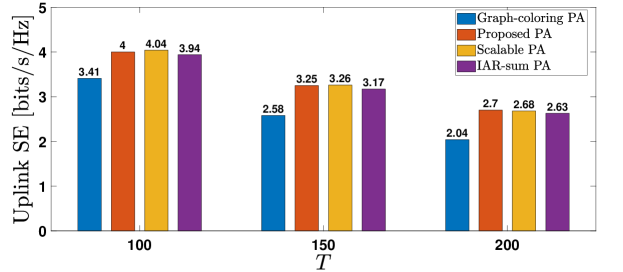
Figure 5: Average uplink SE vs $T$.

IV-B2 Comparison with a distributed scheme

Fig. 6 shows the uplink SE plot for distributed PA schemes. Again in order to decrease the computational costs in distributed survey PA scheme, we have considered the number of UEs to the number of pilots ratio to be $3$. In terms of 90%-likely SE, the proposed scheme outperforms the survey-propagation-based scheme by 2% for $T=45$ and by nearly 4% for $T=60$. Thus, indicating the superiority of our proposed scheme.

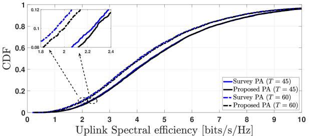
Figure 6: CDF of uplink SE, when $\frac{T}{L_{p}}=3$.

IV-C Discussion

Superior performance of our proposed distributed scheme in terms of both 90%-likely downlink as well as uplink SE demonstrates its ability to outperform not only distributed survey PA scheme, but all of the aforementioned centralized schemes, and performance continues to improve as the number of UE grows. This is primarily attributable to our approach’s priority of reducing pilot contamination for each UE by assigning distinct pilots to UEs that are more susceptible to contamination, thus improving fairness among UEs in terms of contamination. Although our proposed scheme does not focus on improving the average SE, it still achieves greater average downlink as well as uplink SE than IAR-sum and graph-coloring PA schemes in all scenarios. However, our approach has a modest disadvantage in terms of both average downlink and uplink SEs over the scalable PA scheme for low user density scenarios. This minor difference in average SE demonstrates that, despite being distributed, our approach is competitive with centralized approaches.

V Conclusion

Our work shows that the proposed distributed pilot assignment technique in distributed mMIMO systems may substantially enhance spectral efficiency compared to centralized as well as distributed existing schemes. By using a distributed approach, this strategy not only boosts spectral efficiency but also reduces latency and increases the network’s fault-tolerance capability. These findings highlight the importance of using distributed resource allocation algorithms to achieve optimal performance in distributed mMIMO systems. The positive findings of this study illustrate the potential benefits of adopting distributed approaches in future distributed mMIMO network plans and deployments.

References

- [1] H. Q. Ngo, A. Ashikhmin, H. Yang, E. G. Larsson, and T. L. Marzetta, “Cell-free massive MIMO versus small cells,” IEEE Trans. on Wireless Commun., vol. 16, no. 3, pp. 1834–1850, 2017.
- [2] Ö. T. Demir, E. Björnson, L. Sanguinetti et al., “Foundations of user-centric cell-free massive MIMO,” Foundations and Trends® in Signal Processing, vol. 14, no. 3-4, pp. 162–472, 2021.
- [3] P. Aswathylakshmi and R. K. Ganti, “Pilotless uplink for massive MIMO systems,” arXiv preprint arXiv:2305.12431, 2023.
- [4] Z. Chen and E. Björnson, “Channel hardening and favorable propagation in cell-free massive MIMO with stochastic geometry,” IEEE Trans. on Commun., vol. 66, no. 11, pp. 5205–5219, 2018.
- [5] E. Björnson and L. Sanguinetti, “Scalable cell-free massive MIMO systems,” IEEE Trans. on Commun., vol. 68, no. 7, pp. 4247–4261, 2020.
- [6] H. Liu, J. Zhang, S. Jin, and B. Ai, “Graph coloring based pilot assignment for cell-free massive MIMO systems,” IEEE Trans. on Veh. Techno., vol. 69, no. 8, pp. 9180–9184, 2020.
- [7] S. Buzzi, C. D’Andrea, M. Fresia, Y.-P. Zhang, and S. Feng, “Pilot assignment in cell-free massive MIMO based on the hungarian algorithm,” IEEE Wireless Commun. Letters, vol. 10, no. 1, pp. 34–37, 2020.
- [8] S. Chen, J. Zhang, E. Björnson, J. Zhang, and B. Ai, “Structured massive access for scalable cell-free massive MIMO systems,” IEEE Journal on Selected Areas in Commun., vol. 39, no. 4, pp. 1086–1100, 2020.
- [9] W. Zeng, Y. He, B. Li, and S. Wang, “Pilot assignment for cell free massive MIMO systems using a weighted graphic framework,” IEEE Trans. on Veh. Techno., vol. 70, no. 6, pp. 6190–6194, 2021.
- [10] S. Chen, J. Zhang, E. Björnson, and B. Ai, “Improving fairness for cell-free massive MIMO through interference-aware massive access,” IEEE Trans. on Veh. Techno., 2022.
- [11] H. Yu, X. Yi, and G. Caire, “Topological pilot assignment in large-scale distributed MIMO networks,” IEEE Trans. on Wireless Commun., vol. 21, no. 8, pp. 6141–6155, 2022.
- [12] S. Kim, H. K. Kim, and S. H. Lee, “Survey propagation for cell-free massive MIMO pilot assignment,” in 2022 IEEE GC Wkshp. IEEE, 2022, pp. 1267–1272.
- [13] M. Rahmani, M. J. Dehghani, P. Xiao, M. Bashar, and M. Debbah, “Multi-agent reinforcement learning-based pilot assignment for cell-free massive MIMO systems,” IEEE Access, vol. 10, pp. 120 492–120 502, 2022.
- [14] H. Q. Ngo, L.-N. Tran, T. Q. Duong, M. Matthaiou, and E. G. Larsson, “On the total energy efficiency of cell-free massive MIMO,” IEEE Trans. on Green Commun. and Network., vol. 2, no. 1, pp. 25–39, 2017.
- [15] E. G. Larsson, O. Edfors, F. Tufvesson, and T. L. Marzetta, “Massive MIMO for next generation wireless systems,” IEEE Commun. Magazine, vol. 52, no. 2, pp. 186–195, 2014.
- [16] S. Sesia, I. Toufik, and M. Baker, LTE-the UMTS long term evolution: from theory to practice. John Wiley & Sons, 2011.
- [17] E. Björnson, J. Hoydis, L. Sanguinetti et al., “Massive MIMO networks: Spectral, energy, and hardware efficiency,” Foundations and Trends® in Signal Processing, vol. 11, no. 3-4, pp. 154–655, 2017.