Mean-Motion Resonances With Interfering Density Waves

Abstract

In this work, we study the dynamics of two less massive objects moving around a central massive object, which are all embedded within a thin accretion disc. In addition to the gravitational interaction between these objects, the disc-object interaction is also crucial for describing the long-term dynamics of the multi-body system, especially in the regime of mean-motion resonances. We point out that near the resonance the density waves generated by the two moving objects generally coherently interfere with each other, giving rise to extra angular momentum fluxes. The resulting backreaction on the objects is derived within the thin-disc scenario, which explicitly depends on the resonant angle and sensitively depends on the smoothing scheme used in the two-dimensional theory. We have performed hydrodynamical simulations with planets embedded within a thin accretion disc and have found qualitatively agreement on the signatures of interfering density waves by measuring the torques on the embedded objects. By including in interference torque and the migration torques in the evolution of a pair of planets, we show that the chance of resonance trapping depends on the sign of the interference torque. For negative torques the pairs are more likely located at off-resonance regimes. The negative torques may also explain the $1\%-2\%$ offset (for the period ratios) from the exact resonance values as observed in Kepler multi-planet systems.

1 Introduction

Mean motion resonances (MMRs) generally arise for a system with two (or more) point masses orbiting around a common massive object. The mutual gravitational interaction between the two point masses gives rise to resonant dynamics of the resonant degree of freedom of this system when the period ratio is close to $j+k:j$ (Murray & Dermott, 1999), where both $j,k$ are integers. This general setting applies for various astrophysical systems at different scales, including satellites orbiting around planets (Peale, 1976), planets orbiting around stars (Petrovich et al., 2013), and stars/stellar-mass black holes orbiting around supermassive black holes (Yang et al., 2019; Peng & Chen, 2023). For example, it is known that the satellites Mimas and Tethys of Saturn are in a $4:2$ resonance with their mean motions being $n_{\rm M}:n_{\rm Te}=2.003139$ (Murray & Dermott, 2000). The Kepler mission has detected thousands of planets, some of which (although much less than expected) belong to multi-planet systems that exhibit resonant period ratios as well (Lissauer et al., 2012; Fabrycky et al., 2014). On the other hand, the AGN (Active Galactic Nuclei) may capture stellar-mass black holes from the nuclear star cluster through the density wave generation (Tanaka et al., 2002; Tanaka & Ward, 2004). The embedded stellar-mass black holes may be gravitationally captured into binaries within the AGN disc (Li et al., 2023; DeLaurentiis et al., 2023; Rowan et al., 2023b, a; Wang et al., 2023; Whitehead et al., 2023), which subsequently become sources for ground-based gravitational wave detectors (e.g., Li et al., 2021, 2022; Dempsey et al., 2022; Kaaz et al., 2023; Li & Lai, 2022, 2023; Lai & Muñoz, 2023). They may also migrate towards the central massive black hole and eventually become extreme mass-ratio inspirals (EMRIs), which is expected to be an important or even dominant EMRI source for space-borne gravitational wave detectors (Pan & Yang, 2021a; Pan et al., 2021; Pan & Yang, 2021b). If a pair of stellar-mass black holes are trapped into a mean-motion resonance, they may migrate together towards the central massive black hole for certain period of time until the resonance locking breaks down (Yang et al., 2019; Peng & Chen, 2023). This possibly lead to subsequent EMRI events from the same galaxy with relatively short separations and/or gravitational environmental impacts on the EMRI waveform due to the tidal resonance effect (Bonga et al., 2019; Pan et al., 2023).

Starting from an initial state away from the mean-motion resonance, a system may be captured into resonance due to additional dissipation mechanisms, i.e., migration torques from the disc. The probability of resonance capture depends on factors such as the migration direction, the initial orbital eccentricity, the masses of planets and central stars, etc (Murray & Dermott, 1999). In addition, Goldreich & Schlichting (2014) showed that by incorporating migration torques into the long-term evolution of a pair of planets orbiting around a star, it is possible to explain that Kepler has observed much less than $50\%$ multi-planet systems trapped into mean motion resonances . The period ratios for those residing near resonances are slightly larger than the exact resonances values, which is consistent with the requirement that resonance capture requires convergent migration. However, the average $1\%-2\%$ offset from the exact resonance values for the period ratios is difficult to explain within the framework of Goldreich & Schlichting (2014), so that it was conjectured additional mechanism is in operation to deduce the eccentricity and enhance the period ratio offset. There are debated arguments about whether tidal damping can account for the increased period ratio offset (Lithwick & Wu, 2012; Batygin & Morbidelli, 2013; Lee et al., 2013). It has also been suggested that dissipation of density waves near the planets may reverse the migration direction and/or increase the period ratio offset. It is however also worth to note that such mechanism is likely more relevant for massive planets with gap opening on the proto-planetary discs (Baruteau & Papaloizou, 2013).

We notice that when there are multiple planets moving within a disc, the total density wave generated will be a superposition of waves contributed by each planet. In cases where planet orbital frequencies are not commensurate, the interference between different components of density waves only produce an oscillatory flux that averages to zero in time. So it is reasonable to expect to no secular effect associated with interfering density waves in this regime. However, when the planets are trapped in the resonance regime the density waves may stay in phase for an extended period of time so that their interference gives rise to additional angular momentum fluxes. The backreaction should also modify the resonant dynamics of the pair of planets.

In this work we explicitly compute the backreaction on the planets due to interfering density waves assuming a thin-disc scenario. Using a two-dimension disk perturbation theory along with a vertical smoothing scheme, we find that the backreaction torque is an sinusoidal function of the resonant phase angle as analogous to the mutual gravitational interactions. The torque is mainly produced in the regime where the location of a Lindblad resonance overlaps with the orbit of a planet. We find that the sign and magnitude of the torque, however, sensitively depends on the different smoothing schemes used in the two-dimensional theory. This means that the physical torque has to be computed in the three-dimensional setup. In order to further test the predictions of theory, we further carry out two-dimension hydrodynamic simulations of these star$+$planets$+$disc systems using the FARGO3D code (Benítez-Llambay & Masset, 2016). We have focused on a relatively simple case that the outer planet is much more massive than the inner one, and the system is possible to be trapped in a mean-motion resonance as the outer planet migrates inward with a rate faster than the inner planet. By performing the simulations with a pair of planets and with individual planet, we can extract the additional torque due to the interference effect. The result qualitatively agrees with the analytical in terms of the location of the peak torque density, the sign of the torque, with a factor of two difference in the magnitude, which possibly comes from the approximation made in the analytical theory.

With the interference torque included in the orbital evolution of a pair of planets, we find that a positive interference torque generally leads to higher chance of resonance locking, whereas a negative torque tends to produce more pairs of planets with period ratio away from the resonant values. This is interestingly consistent with the fact that the majority of Kepler’s planet pairs are found away from resonant period ratios. We further examine the co-evolution of planet pairs with similar set-ups in Goldreich & Schlichting (2014), in connection to Kepler observations. We find that for the same sets of planets and disc profiles, the interfering density wave terms are able to boost the period ratio offset by more than a factor of four, so that the observed offset level $\sim 1\%-2\%$ is much more compatible with the phenomenological evolution model discussed in Goldreich & Schlichting (2014). Therefore the interfering density waves likely play an important role in the morphology of astrophysical multi-planet systems.

This paper is organized as follows. In Sec. 2 we perform an analytical calculation of the backreaction torque acting on planets due to the interfering density waves, under the thin-disc approximation. We further derive the consequent effect on the change rate of orbital eccentricity and frequency. In Sec. 3 we carry out hydrodynamical simulations of the multi-planet systems embedded within an accretion disc to test the theory of interfering density waves. In Sec. 4 we discuss the modified resonant dynamics due to the interfering density waves, with or without considering the migration torques. In Sec. 5 we discuss the observational signatures of the interfering density waves in connection to the Kepler observations. We conclude in Sec. 6.

2 Interfering Density Waves and their Backreaction

Let us consider multiple objects moving within a thin disc, the gravitational fields of which excite density waves through the Lindblad resonance and the corotation resonance. Density waves carry away energy and angular momentum, which in turn lead to backreaction on the objects as migration torques. These density waves generally have different frequencies as sourced by individual objects, so that the interaction between one object and density waves generated by other objects should be oscillatory, i.e., no secular effect in the long-term evolution. On the other hand, it has been pointed out that density waves may be damped at co-orbital regions of the objects due to dissipation of shocks (Podlewska-Gaca et al., 2012), so that these objects receive additional secular torques by dissipative interaction with density waves. This mechanism is efficient if one or more objects have a partial gap opened to enhance the wave dissipation (Baruteau & Papaloizou, 2013). According to Podlewska-Gaca et al. (2012), the resulting migration direction of planets may be reversed by this effect.

With the dissipative actions (e.g. density wave emission, tides) the multi-body systems may be locked into mean motion resonances, for which the period ratios are close to ratios of integers. As a sample problem we consider an object “A" moving on a fixed outer circular orbit and an object “B" moving along an inner eccentric orbit. The system is locked in a $m:m-1$ resonance such that

$$m\Omega_{A}=m\Omega_{B}-\kappa_{B}$$ (1)

where $\Omega$ is the angular frequency and $\kappa$ is the epicyclic frequency. The density waves produced by object $A,B$ can be decomposed into various harmonics with different azimuthal number and frequencies. Denoting $\varphi^{D}_{s}$ ($s=A,B$) as the gravitational potential perturbation generated by density wave perturbations, they are given by

$$\varphi^{D}_{A}(r)e^{im\phi-i\omega t} =\Phi_{A}e^{i\int^{r}_{A}dsk(s)}e^{im\phi-i\omega t},$$

$$\varphi^{D}_{B}(r)e^{im\phi-i\omega t} =\Phi_{B}e^{i\int^{r}_{B}dsk(s)}e^{im\phi-i\omega t}e^{iQ_{0}}$$ (2)

with $\Phi_{A,B}$ being the amplitudes, $Q_{0}$ being a phase constant, $k$ being the wave number and $\omega=m\Omega_{A}=m\Omega_{B}-\kappa_{B}$. On the other hand, according to the discussion in Goldreich & Tremaine (1979), the angular momentum flux carried by a density wave is

$$\mathcal{F}_{J}=-{\rm sgn}(k)\frac{mr\Phi^{2}}{4G}\left(1-\frac{c^{2}|k|}{\pi G\sigma}\right)$$ (3)

where $\sigma$ is the surface density, $r$ is the radius of wave evaluation, $c^{2}=dP/d\sigma$ is the square of the sound speed and $\Phi$ is the amplitude of the total $\phi^{D}$. Within the thin-disc approximation it can be shown that $\mathcal{F}_{J}$ is independent of $r$. In Goldreich & Tremaine (1979) it is also shown that this angular momentum flux is equal to the migration torque (apart from the opposite sign) that backreacts on the object generating the desntiy wave, which is expected from conservation of the total angular momentum.

With the superposition of density waves from object A and B, the total angular flux at a given radius receives beating terms that is proportional to the amplitudes of both waves. In particular, the beating between the harmonic components described by Eq. 2 leads to a nonzero (average-in-time) cross term

$$\mathcal{F}_{J\times} =-{\rm sgn}(k)\frac{mr}{2G}\left(1-\frac{c^{2}|k|}{\pi G\sigma}\right){\rm Re}(\Phi_{A}\Phi_{B}e^{i(Q_{0}+C_{AB})})\,.$$ (4)

where $C_{AB}$ is the additional phase factor coming from the wave propagation between two objects. This additional angular flux should correspond to additional migration torque acting on the objects, but the angular momentum conservation alone cannot determine the fraction of torque exerted on each object. It requires specific analysis for the value of the torque on each massive object. In addition, it is obvious to see that the phase constant $Q_{0}$ should include the resonant angle $m\lambda_{A}-(m-1)\lambda_{B}-\varpi_{B}$, where $\lambda$ and $\varpi$ are the mean longitude and longitude of pericenter respectively. Because of the dependence on the resonant angle, this additional torque (similar to the gravitational interactions) will introduce qualitatively different modification for the dynamics of the mean-motion resonance, as compared to the type-I migration torques.

2.1 Computing the torque

The individual gravitational field for object A or B can be Fourier-decomposed as ($s=A,B$)

$$\varphi_{s}(r,\phi,t) =\sum^{\infty}_{\ell_{s}=-\infty}\sum^{\infty}_{m_{s}=0}\varphi_{s,\ell_{s},m_{s}}\cos\{m_{s}\phi-[m_{s}\Omega_{s}+(\ell_{s}-m_{s})\kappa_{s}]t\}$$

$$=\sum^{\infty}_{\ell_{s}=-\infty}\sum^{\infty}_{m_{s}=0}\varphi_{s,\ell_{s},m_{s}}\cos\{m_{s}\phi-[\ell_{s}\lambda_{s}-(\ell_{s}-m_{s})\varpi_{s}]\}$$ (5)

where we have used $\Omega_{s}=\dot{\lambda}_{s}$ and $\dot{\varpi}_{s}=\Omega_{s}-\kappa_{s}$ (Goldreich & Tremaine, 1980). The pattern speed of the $\ell_{s},m_{s}$ component is

$$\Omega_{\ell_{s},m_{s}}=\Omega_{s}+\frac{\ell_{s}-m_{s}}{m_{s}}\kappa_{s}\,.$$ (6)

The coefficients $\varphi_{s,\ell_{s},m_{s}}$ as a function of the orbit parameters may be found in Goldreich & Tremaine (1980). In the small eccentricity limit it is proportional to $e^{|\ell_{s}-m_{s}|}$. Therefore up to the linear order in the eccentricity only the $|\ell_{s}-m_{s}|\leq 1$ terms are relevant. As object A is moving on a circular orbit, only $\ell_{s}=m_{s}$ term is nonzero for the expansion of its gravitational potential. The second line of Eq. (2.1) is more general than the first line as it does not assume the time dependent phase to be zero at $t=0$.

The gravitational field of the object A or B resonantly excites density waves in the disc through the Lindblad and corotation resonances, transferring part of the object’s angular momentum to the disc. In particular, the inner and outer Lindblad resonances are located at

$$m(\Omega-\Omega_{\ell,m})=\pm\kappa,\quad m>0\,,$$ (7)

where $m$ specifies the particular Lindblad resonance between the planets, $\Omega,\kappa$ are orbital and epicyclic frequencies of the fluid, which are slightly different from orbital frequencies of the embedded compact objects. Notice that the location of the inner Lindblad resonance should be close to the radius of object B, i.e.,

$$m(\Omega-\Omega_{m,m})=m(\Omega-\Omega_{\rm A})=\kappa\,.$$ (8)

For the corotation resonance the condition is

$$\Omega=\Omega_{\ell,m}\,.$$ (9)

For this particular Lindblad resonance, the relevant terms in the summation of gravitational harmonics in Eq. 2.1 should have $m_{A}=\ell_{A}=m,m_{B}=m,\ell_{B}=m-1$.

The density waves produced by the external gravitational potential $\varphi_{s}$ ($\varphi_{A,m,m}e^{im\phi-i\omega t}$ and $\varphi_{B,m-1,m}e^{im\phi-i\omega t}$) may be characterized by their associated density perturbation $\sigma_{s}(r)e^{im\phi-i\omega t}$ ($\omega:=m\Omega_{A}=m\Omega_{B}-\kappa_{B}$), velocity perturbation $(u_{s}\hat{e}_{r}+v_{s}\hat{e}_{\phi})e^{im\phi-i\omega t}$ and the gravitational perturbation $\varphi^{D}_{s}(r)e^{im\phi-i\omega t}$ (e.g., see Goldreich & Tremaine (1979) for the wave equations governing these variables). In the spirit of Eq. (A7) of Goldreich & Tremaine (1979), the torque of the external potentials $\phi_{A}=\varphi_{A,m,m},\phi_{B}=\varphi_{B,m-1,m}$ acting on the disc is

$$T=-m\pi\int^{\infty}_{0}drr[\phi_{A}(r)+\phi_{B}(r)]{\rm Im}[\sigma_{A}(r)+\sigma_{B}(r)]\,.$$ (10)

As a result, the backreaction of the density wave produced by object A on object B should be

$$T_{B} =m\pi\int^{\infty}_{0}drr\phi_{B}(r){\rm Im}\sigma_{A}(r)$$

$$=-\pi m{\rm Im}\left\{\int^{\infty}_{0}dr\left[\frac{m\phi_{B}\sigma v_{A}}{m\Omega-\omega}+ir\sigma u_{A}\frac{d}{dr}\left(\frac{\phi_{B}}{m\Omega-\omega}\right)\right]\right\}\,$$ (11)

where the second line is similar to Eq. (A8) of Goldreich & Tremaine (1979).

2.1.1 Lindblad resonances

Near a Lindblad resonance we may use a different radial coordinate $x:=-1+r/r_{L}$ with $r_{L}$ being the radius of the Lindblad resonance. It can be obtained by requiring that (see Eq. (7))

$$D=\kappa(r)^{2}-[m\Omega(r)-\omega]^{2}$$ (12)

equals to zero at $r=r_{L}$. In this near zone of the Lindblad resonance, by solving the relevant wave equations the velocity perturbations can be obtained as (Appendix in Goldreich & Tremaine (1979)):

$$u_{A}=-\frac{\kappa}{r_{L}|\mathcal{D}|}\Psi_{A,\ell,m}\int^{\infty}_{0}dt\,{\rm exp}\left[i\left(tx-\frac{\alpha t^{2}}{2\beta}+\frac{t^{3}}{3\beta}\right)\right]$$ (13)

and

$$v_{A}=i{\rm sgn}(\mathcal{D})\frac{2\Omega}{\kappa}u_{A}$$ (14)

where $\mathcal{D}$ is defined as $[rdD/dr]_{r_{L}}$, $\alpha$ is $(2\pi G\sigma r/c^{2})_{r_{L}}{\rm sgn}(k)$, $\beta$ is $(r/c)^{2}_{r_{L}}\mathcal{D}$ and $\Psi_{s,\ell,m}$ is the source term in the wave equation:

$$\Psi_{s,\ell,m}=\left(r\frac{d\varphi_{s,\ell,m}}{dr}+\frac{2m\Omega}{m\Omega-\omega}\varphi_{s,\ell,m}\right)\,.$$ (15)

Here we have selected out the relevant harmonics with azimuthal number $m$ and pattern frequency $\omega$ in Eq. (2.1). Near the mean-motion resonance, although the “pattern frequency" of relevant density waves generated by object A and B are both $\omega$, the wave variables may differ by a phase offset $Q=m\lambda_{A}-(m-1)\lambda_{B}-\varpi_{B}$. If we use object B as the phase reference, there is an additional factor of $e^{-iQ}$ multiplying the right hand side of Eq. (13). In addition, near the Lindblad resonance Eq.(2.1) can be further written as

$$T_{B}=-\frac{\pi m\sigma r_{L}}{\kappa}{\rm sgn}(\mathcal{D})\int^{\infty}_{-\infty}dx\Psi_{B,\ell,m}{\rm Re}(u_{A})f(x)$$ (16)

where the window function $f(x)$ is chosen such that $f=1$ near the resonance location and $f(x)\rightarrow 0$ for $|x|\rightarrow\infty$ to eliminate oscillatory contributions far away. For a single object $s$, the Lindblad toque is given by

$$T_{\rm s}=\frac{\pi^{2}m\sigma\Psi_{s,\ell,m}^{2}}{\mathcal{D}}\,$$ (17)

following the similar procedure in Goldreich & Tremaine (1979).

Let us consider the inner Lindblad resonance of object A, near which $\Psi_{B,\ell,m}$ may be written as (Eq. $52$ in Ward (1988)) after taking into account the vertical average of of the disc (so that the divergence is removed)

$$\Psi_{B,m-1,m}= -e_{B}\frac{GmM_{B}}{a_{B}\sqrt{\pi}}\left(\frac{a_{B}\Omega}{c}\right)[\mathcal{F}_{2}(0,\xi)-4\mathcal{F}_{0}(0,\xi)]$$ (18)

$$+\frac{4}{\pi}\frac{GM_{B}}{h\sqrt{\pi}}\sin f_{c}=\Psi_{d}+\Psi_{c}\sin f_{c}$$

where $M_{B}$ is the mass of object B, $e_{B}$ is its orbital eccentricity, $a_{B}$ is the semi-major axis, $h$ is the disc height and $\xi$ is defined as $\xi=mc/r\Omega$. Notice that for thin discs $c\sim\Omega h=\Omega r(h/r)$ so that $\xi\ll 1$ for low order m. Here $f_{c}$ is related to $r$ as

$$\frac{r}{a_{B}}-1=\gamma_{0}-1=-e\gamma_{0}\cos f_{c}$$ (19)

The contribution from the $\Psi_{c}$ term becomes nonzero if $|1-\gamma_{0}|<e\gamma_{0}$, i.e., $r$ lies between aphelion and perihelion. The definitions of $\mathcal{F}$ functions are expressed as integrals of modified Bessel functions (Eq. 26 of Ward (1988)):

$$\mathcal{F}_{0}(\alpha,\xi) =\pi^{-1}\int^{\infty}_{-\infty}e^{-(t/\xi)^{2}}K_{0}(\sqrt{\alpha^{2}+t^{2}})dt\,,$$

$$\mathcal{F}_{2}(\alpha,\xi) =\pi^{-1}\int^{\infty}_{-\infty}e^{-(t/\xi)^{2}}\left\{\frac{K_{1}(\sqrt{\alpha^{2}+t^{2}})}{\sqrt{\alpha^{2}+t^{2}}}-\frac{\alpha^{2}K_{2}(\sqrt{\alpha^{2}+t^{2}})}{\alpha^{2}+t^{2}}\right\}dt\,.$$ (20)

In the limit that $\xi\ll 1$, we have

$$\mathcal{F}_{2}(0,\xi)\approx\frac{2}{\sqrt{\pi}}\frac{1}{\xi}\,.$$ (21)

With $\Psi_{B,m-1,m}$ and $u_{A}$ the torque operating on object B can be evaluated following Eq. 2.1.1. The torque $T_{B}$ can be explicitly written as

$$T_{B}= \frac{m\pi\sigma}{\mathcal{D}}\Psi_{A,m,m}\int^{\infty}_{-\infty}dxf(x)(\Psi_{d}+\Psi_{c}\sin f_{c})$$

$$\times{\rm Re}\left\{\int^{\infty}_{0}dt\,{\rm exp}\left[i\left(tx-\frac{\alpha t^{2}}{2\beta}+\frac{t^{3}}{3\beta}-iQ\right)\right]\right\}$$ (22)

Notice that the $\Psi_{d}$ term has no explicit $x$ dependence, so it can be moved outside of the integral. By using the relation that (Goldreich & Tremaine, 1979)

$$\int^{\infty}_{-\infty}dx\int^{\infty}_{0}dtf(x){\rm exp}\left[i\left(tx-\frac{\alpha t^{2}}{2\beta}+\frac{t^{3}}{3\beta}\right)\right]$$

$$\approx 2\pi\int^{\infty}_{0}dt\delta(t){\rm exp}\left[i\left(-\frac{\alpha t^{2}}{2\beta}+\frac{t^{3}}{3\beta}\right)\right]=\pi\,,$$ (23)

we can identify the part of torque within $T_{B}$ that is associated with $\Psi_{d}$:

$$T_{\rm Bd}=\frac{\pi^{2}m\sigma\Psi_{A,m,m}\Psi_{d}}{\mathcal{D}}\cos Q\,.$$ (24)

On the other hand, the $\Psi_{c}$ term in the integral of Eq. 2.1.1 has explicit dependence on $x$, which only makes nonzero contribution for the radius inside the orbital range $r\in[a_{B}(1-e),a_{B}(1+e)]$. This part of the integral is equal to ($dx=e\sin f_{c}df_{c}$)

$$T_{Bc}= \frac{m\pi\sigma}{\mathcal{D}}\Psi_{A,m,m}\Psi_{c}\int^{\infty}_{-\infty}dxf(x)\sin f_{c}\Theta[ea_{B}-|r-a_{B}|]$$

$$\times{\rm Re}\left\{\int^{\infty}_{0}dt\,{\rm exp}\left[i\left(tx-\frac{\alpha t^{2}}{2\beta}+\frac{t^{3}}{3\beta}-iQ\right)\right]\right\}$$

$$\approx \frac{m\pi\sigma}{\mathcal{D}}\Psi_{A,m,m}\Psi_{c}\int^{\pi}_{0}e\sin^{2}f_{c}f(x_{0})df_{c}$$

$$\times{\rm Re}\left\{\int^{\infty}_{0}dt\,{\rm exp}\left[i\left(tx_{0}-\frac{\alpha t^{2}}{2\beta}+\frac{t^{3}}{3\beta}-iQ\right)\right]\right\}$$

$$= \frac{m\pi^{2}e\sigma}{2\mathcal{D}}\Psi_{A,m,m}\Psi_{c}{\rm Re}\left[\,W(\alpha,\beta)e^{iQ}\right]$$ (25)

where $x_{0}=a_{B}/r_{L}-1\sim\mathcal{O}(h^{2}/a_{B}^{2})$ so that $f(x_{0})\approx 1$ , and we have defined a function $W(\alpha,\beta):=\int^{\infty}_{0}dt\,{\rm exp}\left[i\left(-\frac{\alpha t^{2}}{2\beta}+\frac{t^{3}}{3\beta}\right)\right]$ for the integral in the last line. Notice that the integral in t becomes highly oscillatory when $t>{\rm Min}[\beta^{1/3},\sqrt{\beta/\alpha}]$, with $\alpha\sim r/h/Q_{t},\beta\sim\mathcal{O}(r^{2}/h^{2})$ ($Q_{t}$ is the Toomre parameter). We expect both $\beta^{1/3}x_{0}\ll 1$ and $\sqrt{\beta/\alpha}x_{0}\ll 1$, so that the $tx_{0}$ term in the integral may be removed. The resulting $T_{\rm B}$ (by including both the $T_{Bd}$ and $T_{Bc}$ components) is

$$T_{\rm B,in}=\frac{\pi^{2}m\sigma\Psi_{A,m,m}}{\mathcal{D}}\left\{\Psi_{d}\cos Q+\frac{e}{2}\Psi_{c}{\rm Re}\left[\,W(\alpha,\beta)e^{-iQ}\right]\right\}\,.$$ (26)

In general the two terms within the bracket together give rise to a sinusoidal term in the resonant angle $Q$. In the solar neighborhood the Toomre parameter is close to one (Goldreich & Tremaine, 1979). If we adopt the same approximation $Q_{t}\sim\mathcal{O}(1)$ as the analysis in Goldreich & Tremaine (1979), we expect $\beta^{1/3}\gg\sqrt{\beta/\alpha}$ and $W(\alpha,\beta)\approx\sqrt{\pi\beta/2\alpha}e^{-i\pi/4}$. In this limit the inner Lindblad torque becomes

$$T_{\rm B,in}=\frac{\pi^{2}m\sigma\Psi_{A,m,m}}{\mathcal{D}}\left[\Psi_{d}\cos Q+\frac{e}{2}\sqrt{\pi\beta/2\alpha}\Psi_{c}\cos(Q+\pi/4)\right]\,.$$ (27)

On the other hand, in the limit that the disk self-gravity is negligible, we expect that $\beta^{1/3}\ll\sqrt{\beta/\alpha}$. In this limit we have

$$W(\alpha,\beta)\approx\left\{\frac{i\Gamma(1/3)}{2\times 3^{2/3}}+\frac{2\pi}{2\times 3^{2/3}\Gamma[2/3]}\right\}\beta^{1/3}\,.$$ (28)

Plugging this expression into Eq. 26 we can obtain the corresponding torque expression

$$T_{\rm B,in}\approx\frac{\pi^{2}m\sigma\Psi_{A,m,m}}{\mathcal{D}}\left[\Psi_{d}\cos Q+0.64e\beta^{1/3}\Psi_{c}\cos(Q-0.52)\right]\,.$$ (29)

For the outer Lindblad resonance of object A, $\Psi_{B,m-1,m}$ is approximately constant in the relevant resonance range, so that

$$T_{\rm B,out}=\frac{\pi^{2}m\sigma\Psi_{A,m,m}\Psi_{B,m-1,m}}{\mathcal{D}}\cos Q\,.$$ (30)

The expression is regular within the thin disc approximation so that the vertical average is not needed. Its value is given by

$$\Psi_{B,m-1,m}=-e\frac{GM_{B}}{2a}\left[\gamma^{2}\frac{d^{2}b^{m}_{1/2}}{d\gamma^{2}}-4m\gamma\frac{db^{m}_{1/2}}{d\gamma}+4m^{2}b^{m}_{1/2}\right]$$ (31)

where $b^{m}_{1/2}(\gamma)$ are the Laplace coefficients

$$b^{m}_{1/2}(\gamma)\equiv\frac{2}{\pi}\int^{\pi}_{0}\frac{\cos m\phi d\phi}{(1-2\gamma\cos\phi+\gamma^{2})^{1/2}}$$ (32)

and the above expression should be evaluated at $\gamma_{0}=[(m+1)/(m-1)]^{2/3}$ in the case of a Keplerian disc. As we compare $\Psi_{B,m-1,m}$ evaluated at the inner and outer Lindblad resonance of object B, we find that $\Psi_{B,m-1,m}$ of the inner Lindblad (e.g. Eq. 18) is larger than the one for outer resonance by a factor $\sim 1/\xi$. So the contribution from outer Lindblad resonance can be neglected for thin discs.

2.1.2 Corotation resonance

For a single object s, the torque due to corotation resonnace is

$$T_{\rm s,co}=-\frac{m\pi^{2}}{2}\left[\left(\frac{d\Omega}{dr}\right)^{-1}\frac{d}{dr}\left(\frac{\sigma}{B_{0}}\right)(\varphi_{s,\ell,m})^{2}\right]$$ (33)

with $B_{0}:=\Omega+r/2d\Omega/dr$. In analogy with the case of Lindblad resonances, the interaction between density wave generated by object A and object B produces a corotation torque:

$$T_{\rm B,co}=-\frac{m\pi^{2}}{2}\left[\left(\frac{d\Omega}{dr}\right)^{-1}\frac{d}{dr}\left(\frac{\sigma}{B_{0}}\right)\varphi_{A,m,m}\varphi_{B,m-1,m}\cos Q\right]_{r_{C}}$$ (34)

evaluated at the location of corotation resonance $r_{C}$. Notice that $\varphi_{A,m,m}$ here needs to be averaged over the vertical scale of the disc, which gives rise to (Ward, 1988)

$$\langle\varphi_{A,m,m}\rangle=-\frac{2GM_{A}\mathcal{F}_{0}(0,\xi)}{r\sqrt{\pi}}\xi^{-1}\,.$$ (35)

Since the factor $\mathcal{F}_{0}(0,\xi)\propto\xi$ for small $\xi$, it means that $\langle\varphi_{A,m,m}\rangle$ has no explicit $\xi$ dependence. On the other hand, we have

$$\varphi_{B,m-1,m}=-e\frac{GM_{B}}{2a}\left[\gamma\frac{db^{m}_{1/2}}{d\gamma}+(1-2m)b^{m}_{1/2}\right]\,.$$ (36)

The resulting $T_{\rm B,co}$ is approximately $\mathcal{O}(\xi^{2})\sim\mathcal{O}(h^{2}/r^{2})$ times smaller than $T_{\rm B,in}$, so we shall neglect this piece in the rest of the discussions.

2.2 Change rate of orbital quantities

The additional torque due to interfering density waves affects the orbital motion of object B. In this section we evaluate the corresponding $\dot{a}$ and $\dot{n}$, where $n$ is the mean motion. We also assume a Keplerian disc profile to simplify the calculations, which may also serve as order-of-magnitude estimation for more general scenarios. For a Keplerian disc we expect

$$\mathcal{D}=3(m-1)\Omega^{2}_{B}\,.$$ (37)

and

$$\frac{\beta}{\alpha}=\frac{3M}{2\pi\sigma a^{2}}\,.$$ (38)

To evaluate the Lindblad torque in Eq. (26) $\Psi_{A,m,m}$ is also required:

$$\Psi_{A,m,m}=-\frac{GM_{A}}{r_{A}}\left[\gamma\frac{db^{m}_{1/2}}{d\gamma}+2mb^{m}_{1/2}\right]_{\gamma}$$ (39)

where $\gamma$ should be set as $\gamma=(1-1/m)^{2/3}$. For a particular $m-1:m$ inner mean-motion resonance between object B and A, only the density waves with the same $m$ is relevant for obtaining the “resonant torque". Let us consider the case with $m=2$ which will be further discussed in Sec. 4:

$$\Psi_{A,2,2}=-2.4\frac{GM_{A}}{r_{A}}\,.$$ (40)

For object B ’s orbit, the change rate of eccentricity due to the additional torque is (Ward, 1988)

$$\frac{1}{e_{B}}\frac{de_{B}}{dt}= \left[\Omega_{m-1,m}-\Omega_{B}-2e_{B}^{2}\Omega_{B}\left(1+\frac{d\log\kappa}{d\log r}\right)_{r=a}\right]$$

$$\times\frac{T}{M_{B}e_{B}^{2}a_{B}^{2}\kappa^{2}}$$ (41)

where we only use the dominant contribution from $T_{\rm B,in}$. At this point, to simplify the discussions, we shall assume that $Q_{t}$ is of order unity. In the case of a Keplerian disc, assuming that $e\ll 1$, the $e^{2}$ term within the square bracket can be neglected and the $\dot{e}$ (for $m=2$) simplifies to

$$\frac{de_{B}}{dt}= \frac{-1}{m}\frac{T_{\rm B,in}}{M_{B}e_{B}a_{B}^{2}\Omega_{B}}\approx\,3\left(\frac{m_{A}}{M}\right)\frac{\sigma a_{B}^{2}}{M}\left(\frac{a_{B}}{h}\right)^{2}\Omega_{B}$$

$$\times \left[\frac{h}{a_{B}}\sqrt{\frac{3M}{4\pi\sigma a_{B}^{2}}}\cos(Q+\pi/4)-\cos Q\right]$$

$$:= \frac{\cos(Q+\pi/4)}{\tau_{+}}-\frac{\cos(Q)}{\tau_{0}}$$ (42)

so that the sign of $\dot{e}$ depends on the relative magnitude of the $\cos Q$ and $\cos(Q+\pi/4)$ term. In order to compute $n$, we use the energy balance equation that

$$\frac{dE}{dt}=\Omega_{B}T_{\rm B,in}$$ (43)

which naturally leads to

$$\dot{n}/n =-3(GM)^{-2/3}n^{1/3}M_{B}^{-1}T_{\rm B,in}$$

$$:=\frac{6e\cos(Q+\pi/4)}{\tau_{+}}-\frac{6e\cos(Q)}{\tau_{0}}\,.$$ (44)

Notice that the ratio between $\tau_{+}$ and $\tau_{0}$ is

$$\frac{\tau_{0}}{\tau_{+}}=\sqrt{\frac{3Q_{t}}{4}\frac{h}{a_{B}}}\,.$$ (45)

For thin discs with $h/a\ll 1$, the $\tau_{+}$ term is subdominant comparing to the $\tau_{0}$ term so that it may be neglected in the equation of motion. This is the assumption we adopt in the discussion in Sec. 4. However, in more general settings $W(\alpha,\beta)$ needs to be evaluated numerically to obtain the torque and the corresponding decay rate.

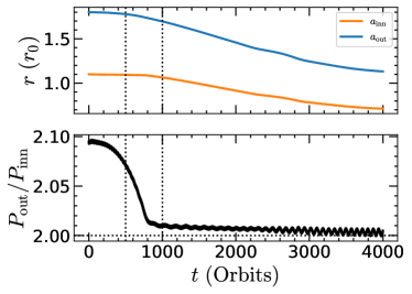
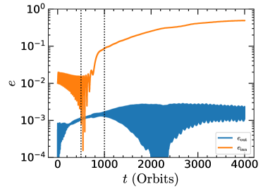
Figure 1: Left panels: the semi-major axis (upper left) and orbital period ratio (lower left) evolution for a pair of planets with $\mu_{B}=10^{-5}$ and $\mu_{A}=3\times 10^{-4}$. The planet pair is captured into 2:1 MMR around 800 orbits. Right panel: the orbital eccentricity evolution for the planet pair. The two vertical dotted lines show 500 and 1000 orbits just before and after the 2:1 MMR. Note that all the times in this figure are measured in unit of the orbital period at $r=r_{0}$.

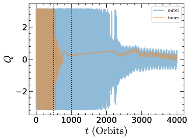
Figure 2: The resonance angle evolution for the inner object and the outer one. The inner object shows a finite resonance angle around 1000 orbits while the outer object still circulates around the full orbital phase (The resonant angle for the outer resonance is defined as $Q=2\lambda_{A}-\lambda_{B}-\varpi_{A}$). The two vertical dotted lines show 500 and 1000 orbits just before and after the 2:1 MMR, same as Figure 1. Note that all the times in this figure are measured in unit of the orbital period at $r=r_{0}$.

3 Hydrodynamical simulations

In order to further demonstrate the effect of interfering density waves beyond the analytical calculations, a few hydrodynamical simulations are carried out to confirm the effect of interfering density waves on the dynamics of the MMR pair. We use the FARGO3D code (Benítez-Llambay & Masset, 2016) to simulate the gravitational interaction of a pair of planet with a disc. The disc aspect ratio is approximately $h/r=0.05(r/r_{0})^{0.5}$, which leads to a constant temperature profile over the disc. The surface density is set as $\sigma=10^{-4}M/r_{0}^{2}$ at $r=r_{0}$, and is constant over the entire disc, where $M$ is the stellar mass, $r_{0}$ is the typical length scale of the disc, which can be scaled freely to compare with observations. We also assume an $\alpha$-prescription for the gas kinematic viscosity $\nu=\alpha h^{2}\Omega$ (Shakura & Sunyaev, 1973). A moderate $\alpha=0.01$ is adopted to ensure that both planets do not open deep gaps in the disc.

A pair of planets is initialized at $r_{\rm p,B}=1.1r_{0}$ and $r_{\rm p,A}=1.8r_{0}$. The inner planet has a finite eccentricity of $e_{\rm p,B}=0.01$, while the outer one moves along a circular orbit. Both planets are allowed to freely evolve subjected to the planet-disc interaction and the mutual gravitational interaction between the planets. The mass ratio of the inner and outer planet with the host star is chosen as $\mu_{\rm B}=10^{-5}$ and $\mu_{\rm A}=3\times 10^{-4}$, so that the inner planet is much lighter than the outer one. The potential of the planet pair and the host star is described as

$$\phi= - \frac{GM}{\left|\bm{r}\right|}$$

$$+ \sum_{i=\rm A,B}\left[-\frac{G\mu_{i}M}{(\left|\bm{r}_{{\rm p},i}-\bm{r}\right|^{2}+\epsilon^{2})^{1/2}}+\mu_{i}\Omega_{{\rm p},i}^{2}\bm{r}_{{\rm p},i}\cdot\bm{r}\right],$$

where the first term represents the potential due to the host star. In addition, the first term in the bracket is the direct potential from each planet, and the second term in the bracket is the indirect potential arising from our choice of coordinate system. We apply a gravitational softening, with length scale $\epsilon=0.6h$, to each planet’s potential.

This particular choice of gravitational potential $\phi$ commonly used in hydrodynamical simulations removes the apparent singularity in evaluating $\Psi_{B,m-1,m}$ at the inner Lindblad resonance, which is instead achieved by introducing a vertical average in Ward (1988) and in the previous section. In order to compute $\Psi_{B,m-1,m}$ in this case, we still use the formula

$$\tilde{\Psi}_{B,m-1,m}=-\frac{GM_{B}e_{B}}{2a_{B}}\left[\gamma^{2}\frac{d^{2}\tilde{b}^{m}_{1/2}}{d\gamma^{2}}-4m\gamma\frac{d\tilde{b}^{m}_{1/2}}{d\gamma}+4m^{2}\tilde{b}^{m}_{1/2}\right]$$ (47)

where we replace $b^{m}_{1/2}$ by its modified version $\tilde{b}^{m}_{1/2}$ (Duffell & Chiang, 2015)

$$\tilde{b}^{m}_{1/2}(\gamma)\equiv\frac{2}{\pi}\int^{\pi}_{0}\frac{\cos m\phi d\phi}{(1-2\gamma\cos\phi+\gamma^{2}+\epsilon^{2}/a^{2}_{B})^{1/2}}\,.$$ (48)

Notice this treatment (Duffell & Chiang, 2015) is presumably obtained in the small eccentricity limit (so that integrals are expanded out in powers of $e_{B}$), whereas here the $e_{B}a_{B},h,\epsilon$ are all on the same order. A more detailed analysis may be required to numerically evaluate $\Psi_{B,m-1,m}$ for this system. Nevertheless, if we still follow the treatment in Duffell & Chiang (2015), $\Psi_{B,m-1,m}$ is a constant with no dependence on $f_{c}$ and the corresponding inner Lindblad torque is

$$T_{\rm B,in}=\frac{\pi^{2}m\sigma\Psi_{A,m,m}}{\mathcal{D}}\tilde{\Psi}_{B,m-1,m}\cos Q\,.$$ (49)

We resolve the disc with a uniform radial grid of $n_{r}=256$ points in a radial domain between $[0.4,4.0]r_{0}$, and a uniform azimuthal grid with $n_{\phi}=512$ points. A convergence test with higher resolutions $[n_{r},n_{\phi}]=[512,1024]$ and smaller radial inner edged has been performed, which does not show significant impact on the dynamics of the planet pair.

Two wave-killing zones are applied at the both the inner and outer radial edge to remove waves near both boundaries (de Val-Borro et al., 2006).

The orbital semi-major axis and the period ratio evolution for the planet pair are shown in the left panel of Figure 1. The planet pair is quickly captured into the 2:1 MMR around 800 orbits, which is accompanied with a damping of the initial eccentricity of the inner planet, as shown in the right panel of Figure 1. Note that the times in the plots are always measured in unit of the orbital period at $r=r_{0}$. After that, the eccentricity of the inner planet is excited during the MMR stage. Specifically, the eccentricity of the inner planet is $e_{\rm B}\simeq 0.006$ around 500 orbits and $e_{\rm B}\simeq 0.08$ around 1000 orbits . The resonance angles of the planet pair are shown in Figure 2, which confirms that the inner object is in 2:1 MMR after 800 orbits, although the resonance angle of the outer one still circulates across the full $2\pi$ range until $\sim 2000$ orbits.

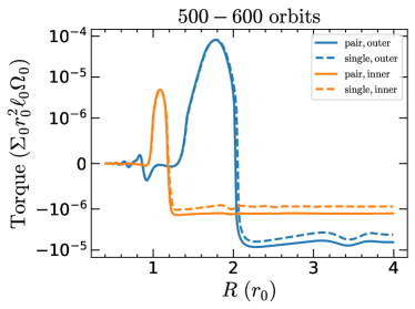
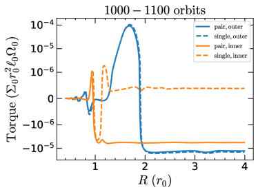
Figure 3: The cumulative gravitational torque on the embedded objects as a function of $R$ for different models. The cumulative torque is obtained by integrating the differential torque density over $R$ from the inner boundary to a given $R$, so the total gravitational torque for each embedded object is the value at the large enough $R$ (e.g., $R>3r_{0}$). The solid lines show the torques calculated from the planet pair simulations, while the dashed lines show the torque from the single planet case. Different colors correspond to different components of the planet pair. All the torque calculations are time-averaged within 500-600 orbits (left panel) or 1000-1100 orbits (right panel), which correspond to the stage just before and after the MMR of the planet pair simulations. We can see that the single planet simulation can well reproduce the torques in the planet pair simulations before the MMR, while after the planet pair being captured into MMR, there exists significant torque difference for the inner object between the single planet and planet pair simulations which should be due to the interfering term.

We can then use the torque acting on each object to probe the existence of interfering density waves, as motivated by Eq. 49. To this end, we also run a few single planet simulations with their orbit fixed in time. Two sets of single planet simulations have been performed, with one to compare with the planet pair case at 500 orbits, and another to compare with the case at 1000 orbits, i.e., before and after the MMR for the inner planet. For each set of single planet simulations (e.g., the set at 500 orbits), we have two individual simulations, where one massive planet is located at the outer orbit and the other less massive one is located at the inner orbit. The planet semi-major axis and the orbital eccentricity are initialized with the same values from the planet pair simulation at that time (e.g., the set at 500 orbits).

We can then calculate the torques on the inner and outer planets for both the single planet and planet pair simulations. The left and right panels of Figure 3 show the radial distribution of cumulative torque on the inner and outer planets before and after the MMR. The solid lines correspond to the cases for the planet pair simulations, while the dashed lines are the cases for the single planet simulations. The surface density at the inner planet location could be modified by the outer object for the planet pair case. To make a fair comparison with the single planet simulation, one should also consider the surface density modification at the single planet location arisen from the other embedded object. But we have confirmed that this effect is actually negligible. To avoid the torque oscillation due to the small orbital eccentricity ($e\lesssim 0.08$ for $t<1000$ orbits), a time-averaging for the torques over 100 orbits is done around 500 and 1000 orbits. At 500 orbits, we can see that the torques on each planet from the planet pair case are quite consistent with the single planet cases, which confirms that there are indeed no additional interfering density wave terms on the other planet when the planet pair are out of MMR. At 1000 orbits, however, there is remarkable difference for the torque on the inner planet between the planet pair and single planet cases, although these two are still consistent with each other for the outer planet. This is well consistent with expectation that the $Q$-dependence of the interfering term as shown in Eq. 49, i.e., the time-average $\langle\cos Q_{\rm A}\rangle$ is zero when out of MMR, while this term cannot be diminished for the finite $Q$ in MMR case.

The difference of the torque between the planet pair and single planet cases shown in the right panel of Figure 3 can then be used to compare with the analytical theory for the additional torque associated with the interfering density wave. In the limit of the disk self-gravity is negligible, our analytical theory predicates that the additional torque from the interfering density wave can be estimated based on Eq. 49 assuming a Keplerian disk, which is $T_{\rm B,in}\sim-2.5\times 10^{-6}$ (in code unit) using the model parameter from the simulation. The torque due to the interfering density wave for the inner planet measured directly from simulation can be calculated from the torque difference of the planet pair and single planet (the difference between the solid and dashed orange lines in the right panel of Figure 3), which is about $\sim-5.5\times 10^{-6}$ (in code unit). This is about a factor of 2 larger in magnitude than that expected from our analytical theory, although the sign of this torque difference, the location of the torque jump (i.e., at the location of inner Lindblad resonance) and the fact that main effect comes from the coupling between the gravity of planet B and disk perturbations generated by planet A is well consistent with our theory. We do not fully understand the origin(s) of discrepancy in torque magnitude. One possible source may arise from the small eccentricity approximation assumed in obtaining $\tilde{\Psi}_{B,m-1,m}$ and Eq. 49. The backreaction of planet B to the local disk profile seems to be small in the current set-up. Nevertheless, it is fair to state that the numerical simulation qualitatively agrees with the simplified analytical theory.

On the other hand, the analytical theory in the previous section uses “ad hoc" vertical average prescription following Ward (1988), so that the apparent divergence in $\Psi_{B,m-1,m}$ in the two-dimensional theory can be regularized. If we were to apply $\Psi_{B,m-1,m}$ in Eq. 29 we would obtain $T_{\rm B,in}\sim 10^{-6}$ in code unit, which is positive. The fact these two different smoothing schemes in the two-dimensional theory giving quite different predictions in the backreaction torque means that the actual physical torque may sensitively depend on the local three-dimensional disk structure. A more accurate treatment should be solving the three-dimensional model and considering the vertical modes similar to the analysis in Tanaka & Ward (2004). This calculation is beyond the scope of this work and the resulting torque corresponds to an effective $\tau_{0}$ which may be either positive or negative.

4 Modified Resonant Dynamics

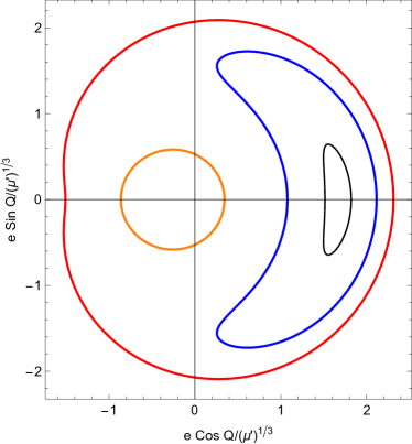
Figure 4: The phase space trajectories of a $2:1$ resonance with $k=2k_{\rm crit}$.

As discussed in Sec. 2, for a pair of massive objects embedded in an accretion disc and trapped within a mean-motion resonance, the interfering density waves produces a backreaction torque that depends on the resonant angle $Q$. Such $Q$-dependence likely introduces qualitatively different resonant dynamics from those systems involving only gravitational interactions, or those only include constant (in the resonant angle) migration torques. We address the associated dynamical signatures in this section.

Without including the torque from interfering density waves, the equations of motion for the pair of objects considered in Sec. 2 has already been discussed in Goldreich & Schlichting (2014), in which case the outer object A stays at a fixed circular orbit ($\dot{r}_{A}=0$) and the inner object B migrates outwards. The equations of motion including the effect of interfering density waves for $n=\dot{\lambda}_{B},e$ are

$$\dot{n} =3(m-1)\beta_{0}\mu^{\prime}en^{2}\sin Q-\frac{n}{\tau_{n}}+p\frac{e^{2}n}{\tau_{e}}-\frac{6en\cos Q}{\tau_{0}}$$

$$\dot{e} =\beta_{0}\mu^{\prime}n\sin Q-\frac{e}{\tau_{e}}-\frac{\cos Q}{\tau_{0}}$$ (50)

where $\beta_{0}$ is approximately $0.8(m-1)$, $\mu^{\prime}:=M_{A}/M,\mu:=M_{B}/M$, the $p$-related term may be contributed by remote first-order Lindblad resonances and corotation resonances. For illustration of principles we take the same value $p=3$ as used in Goldreich & Schlichting (2014). On the other hand, the change rate of mean motion and eccentricity due to single-body migration torques approximately scale as

$$\frac{1}{\tau_{n}}\sim\mu\frac{\sigma a^{2}}{M}\left(\frac{a}{h}\right)^{2}n,\quad\frac{1}{\tau_{e}}\sim\mu\frac{\sigma a^{2}}{M}\left(\frac{a}{h}\right)^{4}n\,.$$ (51)

The resonant dynamics can be determined by combining Eq. 4 with the definition that $Q=m\lambda_{A}-(m-1)\lambda_{B}-\varpi_{B}$ and the equation of motion for $\varpi_{B}$:

$$\dot{\varpi}_{B}=-\frac{\beta_{0}\mu^{\prime}}{e}n\cos Q\,.$$ (52)

4.1 Without constant migration torques

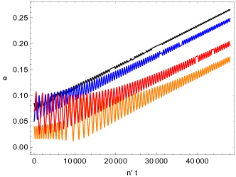
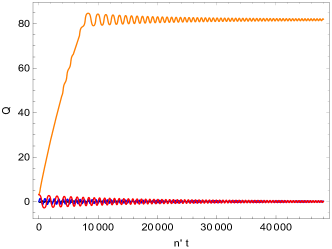
(a)

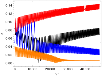
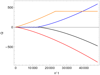
(b)

Figure 5: The evolution of the four trajectories presented in Fig. 4 with $\tau_{0}\beta_{0}\mu^{\prime}n^{\prime}=20$ (top panel) and $\tau_{0}\beta_{0}\mu^{\prime}n^{\prime}=-20$ (bottom panel). The color scheme is chosen such that it is consistent with the phase-space trajectories in Fig. 4 as initial data.

Let us first consider the case with the normal migration torques turned off, i.e. removing $\tau_{e},\tau_{n}$-related terms in Eq. 4. Although this assumption is made to present a simplified discussion on the resonant dynamics, it becomes a reasonable approximation if $\mu^{\prime}\gg\mu$, although in this case $n^{\prime}$ is generally time-dependent. If the $\tau_{0}$-related term is also absent, the equations of motion is compatible with the resonant Hamiltonian (Goldreich & Schlichting, 2014):

$$\mathcal{H}=ke^{2}-\frac{3}{4}(m-1)^{2}e^{4}+2\beta_{0}\mu^{\prime}e\cos Q$$ (53)

with

$$k:=\frac{3}{2}(m-1)^{2}e^{2}-\frac{\beta_{0}\mu^{\prime}}{e}\cos Q+\frac{\dot{Q}}{n}$$ (54)

being a constant in time. The conjugate canonical variables are $Q$ and $e^{2}$. Defining a critical $k$ as $k_{\rm crit}=3^{4/3}((m-1)\beta_{0}\mu^{\prime})^{2/3}/2$, the phase space contains one stable fixed point for cases with $k<k_{\rm crit}$ and two fixed points plus one unstable fixed point for $k>k_{\rm crit}$ (Murray & Dermott, 1999; Goldreich & Schlichting, 2014). In Fig. 4 we show several representative phase space trajectories in terms of a set of re-scaled canonical variables $\{e\cos Q/\mu^{\prime 1/3},e\sin Q/\mu^{\prime 1/3}\}$. The blue and black curves are “libration" trajectories around a fixed point at $e_{\rm max}\approx 1.96(\beta_{0}\mu^{\prime})^{1/3}$ on the positive side of the real axis. The red curve is a large “rotation" orbit. The orange curve is a “rotation" trajectory around the other stable fixed point at $e_{\rm min}\approx 0.093(\beta_{0}\mu^{\prime})^{1/3}$ on the negative side of the real axis.

Now with the $\tau_{0}$ term included, it contributes to another $Q$-dependent driving source that has $90$-degree offset from the mutual gravitational interaction. The ratio of magnitudes is

$$\frac{1}{|\tau_{0}\beta_{0}\mu^{\prime}n|} \sim 0.4\left(\frac{\sigma a^{2}/M}{10^{-3}}\right)\left(\frac{a/h}{10}\right)^{2}$$

$$\sim\left(\frac{\alpha}{0.1}\right)^{-1}\left(\frac{\dot{M}}{0.1\dot{M}_{\rm Edd}}\right)^{-3}\left(\frac{M}{10^{5}M_{\odot}}\right)\left(\frac{a}{10^{3}M}\right)^{5.5}$$ (55)

which may be comparable to one depending on the properties of the disc and the location of the object, so that the resonant dynamics may be significantly affected. In the first line we have noticed that a significant fraction of protoplanetary discs in the Lupus complex observed by the Atacama Large Millimeter/Submillimeter Array has disc gas mass to star mass ratio around $10^{-3}$ (Ansdell et al., 2016). In the second line we have assumed a $\alpha$ disc profile around a supermassive black hole (Kocsis et al., 2011), with $\dot{M}$ being the accretion rate of the central black hole and $\dot{M}_{\rm Edd}$ being the Eddington accretion rate.

In Fig. 5 we present the evolution in the regime that $|\mu^{\prime}n\tau_{0}|\gg 1$, so that the force due to interfering density waves is much weaker than the gravitational interactions between the two objects. In addition, as discussed in the Sec. 3, the sign of the backreaction torque depends on the detail three-dimensional structure of the gas flow near the inner Lindblad resonance, which is not resolved in this study. As a result, we consider two cases with $\tau_{0}\beta_{0}\mu^{\prime}n^{\prime}=\pm 20$ respectively. One common feature of these two scenarios is that the numerical evolution no longer preserves the area in the phase space of the canonical variables, so the evolution is no longer Hamiltonian.

In the case that $\tau_{0}\beta_{0}\mu^{\prime}n^{\prime}=20$, we find various initial data all lead to an asymptotic libration state with increasing eccentricity. In fact, on the right hand side of the $\dot{e}$ equation in Eq. 4, the time average of $\beta_{0}\mu^{\prime}n\sin Q$ is slight larger than the time average of $\cos Q/\tau_{0}$, so that the libration regime drifts towards to the right. On the other hand, in the case that $\tau_{0}\beta_{0}\mu^{\prime}n^{\prime}=-20$, we find different kinds of final states. For the black and red trajectories, the system evolve to a rotation state around the origin with increasing eccentricity in time (similar to the red curve in Fig. 4 with increasing amplitude). The blue trajectory instead lands on another rotation state with shrinking eccentricity in time (similar to the orange curve in Fig. 4 with decreasing amplitude).

Mathematically we can approximately describe the end state of the black and red trajectory as follows. Without the $\tau_{0}$-related terms, the rotational orbits around the origin can be written as

$$n =n_{0}+\epsilon\delta n\cos Q+\mathcal{O}(\epsilon^{2}),$$

$$e =e_{0}+\epsilon\delta e\cos Q+\mathcal{O}(\epsilon^{2}),$$

$$Q =\omega_{0}t+\mathcal{O}(\epsilon)$$ (56)

where $\epsilon$ is a book-keeping parameter and we only keep terms up to the linear order in $\epsilon$. In addition, according to the fact that

$$\dot{Q}=mn^{\prime}-(m-1)n+\frac{\beta_{0}\mu^{\prime}}{e}\cos Q\,,$$ (57)

we can immediately identify that $\omega_{0}=mn^{\prime}-(m-1)n_{0}$. Together with Eq. 4 (with $\tau_{0},\tau_{n},\tau_{e}$-related terms removed), we find that

$$\delta n =-\frac{3(m-1)\beta_{0}\mu^{\prime}e_{0}n^{2}_{0}}{\omega_{0}},$$

$$\delta e =-\frac{\beta_{0}\mu^{\prime}n_{0}}{\omega_{0}}\,.$$ (58)

In order to describe the secular evolution, we can use the evolution of conserved quantities $k,\mathcal{H}$:

$$\frac{dk}{dt} =3e\dot{e}_{\tau_{0}}-\frac{2n^{\prime}}{n^{2}}\dot{n}_{\tau_{0}}=\frac{3e\cos Q}{\tau_{0}}\,,$$

$$\frac{d\mathcal{H}}{dt} =e^{2}\frac{dk}{dt}+\frac{de^{2}}{dt}\left(k-\frac{3}{2}e^{2}+\beta_{0}\mu^{\prime}/e\cos Q\right)$$

$$=\frac{3e^{3}\cos Q}{\tau_{0}}-\frac{2e\cos Q}{\tau_{0}}\left(k-\frac{3}{2}e^{2}+\beta_{0}\mu^{\prime}/e\cos Q\right)$$

$$=-\frac{2e\cos Q}{\tau_{0}}\left(k-3e^{2}\right)-\frac{2\beta_{0}\mu^{\prime}\cos^{2}Q}{\tau_{0}}\,.$$ (59)

After plugging the approximate solution in Eq. 4.1 and Eq. 4.1 and performing average over oscillation cycles in the resonant phase $Q$, we find that (with $m=2$)

$$\langle\dot{k}\rangle=-\frac{3\mu^{\prime}\beta_{0}n_{0}}{\omega_{0}\tau_{0}}\left(1+\frac{3n_{0}e^{2}_{0}}{2\omega_{0}}\right),$$ (60)

which is also useful for the analysis in Sec. 5. On the other hand, the orange curve eventually evolves to a state that

$$\beta\mu^{\prime}n\sin Q\approx\frac{\cos Q}{\tau_{0}}\,,$$

$$mn^{\prime}-(m-1)n+\frac{\beta\mu^{\prime}}{e}n\cos Q\approx 0\,,$$ (61)

i.e., $\dot{e},\dot{Q}\approx 0$, so that the quasi-stationary values of $e,Q$ can be determined as functions of $n$. Notice that here $n$ is still time dependent according to Eq. 4 (with $1/\tau_{e},1/\tau_{n}$ set to be zero), so that this point drifts in time. In addition, from the second line of Eq. 4.1 one can find that at equilibrium the offset of period ratio $mn^{\prime}/n-(m-1)$ is inversely proportional to the eccentricity, i.e., smaller eccentricity corresponds to larger offset of the period ratio (see also the related discussion in Sec. 3). This is a rather general point as long as $Q$ is bounded.

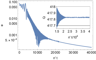
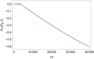
(a)

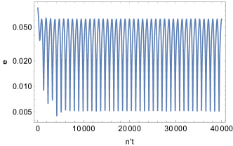
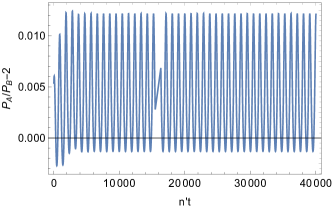
(b)

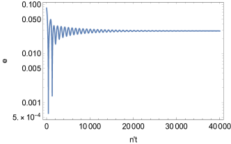
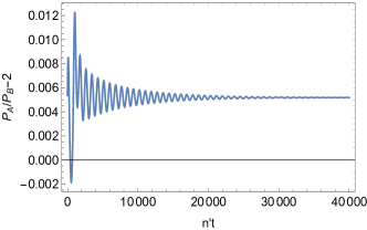
(c)

Figure 6: The evolution of eccentricities and periods with $\tau_{e}=\tau_{n}/50$ (top row), $\tau_{e}=\tau_{n}/100$ (middle row) and $\tau_{e}=\tau_{n}/200$ (bottom row) respectively, according to Eq. 4 but with $\tau_{0}$ terms turned off. The scaled mass of object A is assumed to be $\mu^{\prime}=10^{-4}$ and $\tau_{n}$ is set to be $n^{\prime}\tau_{n}=10^{5}$. The insect of panel (a) shows the evolution of the resonant angle $Q$, which is bounded at late times.

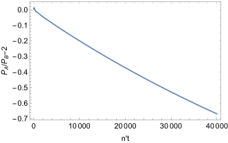
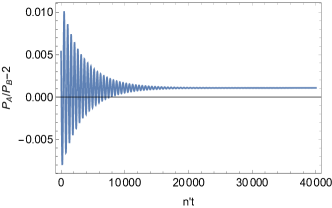
(a)

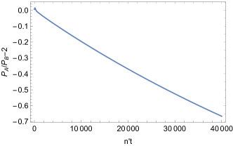
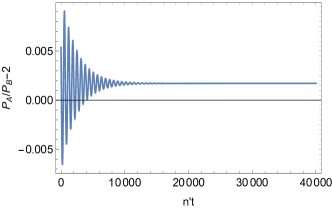
(b)

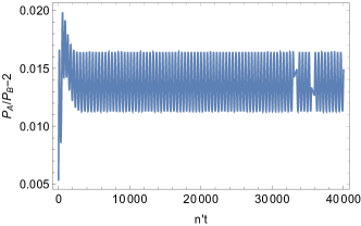
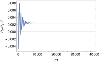
(c)

Figure 7: Similar set up as Fig. 6 but with $\tau_{0}$ set to be $-\tau_{n}/10$ on the left column and $\tau_{n}/10$ on the right column.

4.2 With migration torques

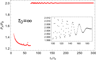
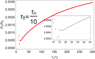
(a)

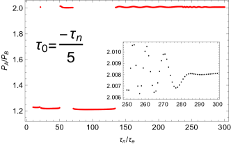
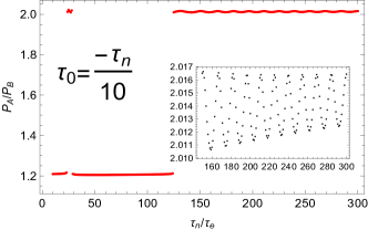
(b)

Figure 8: The end state at $n^{\prime}t=5\times 10^{4}$ where the period ratios are extracted for various $\tau_{0}$. The inset for each plot provides a zoomed-in illustration for the finite amplitude libration regime and the possible fixed point regime.

With the results from Sec. 4.1 we can now discuss evolutions in the more general settings, with the migration torques turned on. In Goldreich & Schlichting (2014) with no $\tau_{0}$-related terms in the equation of motion, it is shown that there are three parameter regimes of interest. The system is trapped in resonance with fixed $Q$ and $e$ for

$$\mu^{\prime}>\frac{(m-1)}{\sqrt{3}m^{3/2}\beta_{0}}\left(\frac{\tau_{e}}{\tau_{n}}\right)^{3/2}$$ (62)

and for

$$\mu^{\prime}<\frac{(m-1)^{2}}{8\sqrt{3}m^{3/2}\beta_{0}}\left(\frac{\tau_{e}}{\tau_{n}}\right)^{3/2}$$ (63)

the system is trapped in resonance in finite duration $\sim\tau_{e}$. When the resonance locking breaks down the system evolves with monotonically changing period ratios and decreasing eccentricities. Between these two limits the system asymptotes a state with finite libration amplitude. Notice that the actual transition between resonance locking and rotational orbits in the phase space may significantly differ from the analytical criteria in Eq. 63 for small $\mu^{\prime}$ and/or $\tau_{n}$, because the adiabatic approximation used to derive the analytical formulas may break down (Goldreich & Schlichting, 2014).

In Fig. 6 we present the evolution of a pair of planets according to Eq. 4 but with the interfering density waves terms neglected. These figures essentially show the same qualitative features as Fig. $5$ in Goldreich & Schlichting (2014). In the top row where $\tau_{e}=\tau_{n}/50$, the system exits the resonance within $\sim\tau_{e}$ timescale and follows with monotonic period ratios afterwards. Notice that although the period ratio is monotonically changing in this regime, we find that the resonant angle $Q$ is bounded (also see related discussion in Sec. 3). This is because the contribution from $mn^{\prime}-(m-1)n$ is canceled with $\dot{\varpi}_{B}$. It is also particularly interesting because if $Q$ stays bounded, the interfering density wave effect stays in operation even if the period ratio is out of resonance-locking, as discussed in Sec. 3. In the middle row with $\tau_{e}=\tau_{n}/100$, the system undergoes finite amplitude libration in the phase spacetime, so that both the eccentricity and period ratio oscillates around a fixed value. In the bottom row with $\tau_{e}=\tau_{n}/200$, the system asymptotes to a state with a fixed eccentricity $\sim 0.03$ and a period ratio offset $\sim 0.005$.

With the $\tau_{0}$ terms included, the evolution may be modified significantly. In Fig. 7 we present the case with the same parameters as in Fig. 6 but with $\tau_{0}=\pm\tau_{n}/10$. For the positive $\tau_{0}$ cases, the system preferably lends on an asymptotic state with constant resonant angle and eccentricity (not shown in the plot). The period ratios are also asymptotically constant with $\leq 0.3\%$ difference from $2$. On the other hand, for the negative $\tau_{0}$ case, the system no longer exhibits finite amplitude libration as shown in panel (c,d) of Fig. 6, but instead loses the resonance locking without keeping bound $Q$. The period ratios are monotonically decreasing for the cases with $\tau_{e}=\tau_{n}/50$ and $\tau_{e}=\tau_{n}/100$, but oscillating around a fixed value for $\tau_{e}=\tau_{n}/200$. In the latter case the phase-space trajectory is qualitatively similar to the red trajectory in Fig. 4. Based on this particular system setup, it seems negative $\tau_{0}$ more likely drives the system far away from resonant period ratios, which is a phenomenon to be understand from the Kepler observations (Deck & Batygin, 2015).

In order to understand the “end state" of the system with the influence of $\tau_{0}$ terms for a larger range of parameters, we perform a series of numerical evolutions using Eq. 4 but with different $\tau_{e}$ and $\tau_{0}$. For each set of evolution we extract the period ratio at the end of the simulation, with $t_{\rm end}n^{\prime}=5\times 10^{4}$. In the top left panel of Fig. 8, such an evolution is shown for $1/\tau_{0}=0$. We find that roughly between $\tau_{n}/\tau_{e}\sim 180$ and $\tau_{n}/\tau_{e}\sim 70$ the “end-state" period ratios show variations at the fixed end-state time, which is the consequence of finite-amplitude libration (i.e., the middle panel of Fig. 6). With smaller $\tau_{n}/\tau_{e}$ than $70$ the period ratio is significantly smaller than 2, which corresponds to the non-resonant regime. On the other hand, for $\tau_{n}/\tau_{e}>180$, the period ratio barely oscillates, which corresponds to the fixed point regime.

As the negative $\tau_{0}$ terms are included, the transition between the non-resonant regime and the libration regime shifts to lower $\tau_{n}/\tau_{e}$, as we can find for the cases with $\tau_{0}=-\tau_{n}/10,-\tau_{n}/5$. In addition, as $|1/\tau_{0}|$ increases, a new non-resonant regime appears in the middle of the regime with roughly constant period ratios, as shown in panel (c,d) of Fig. 8. The presence of additional non-resonant regimes is consistent with our earlier observation that negative $\tau_{0}$s tend to drive more system configurations away from the resonant period ratios. On the other hand, for positive $\tau_{0}$, i.e., $\tau_{0}=\tau_{n}/10$ as shown in the panel (b), most of the parameter range correspond to a system in resonance locking. Positive $\tau_{0}$ likely enhances the chance of resonance locking. In summary, the inclusion of $\tau_{0}$ terms in the evolution equations gives rise to more complex structures in the parameter phase space of such pairs of planets.

5 Observational Implications

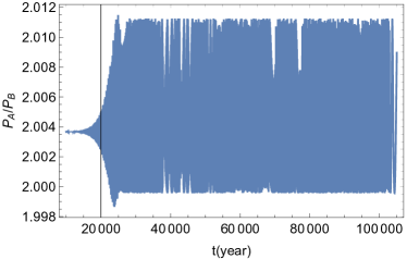
Figure 9: The period ratio of the evolution of a pair of planets with $\mu_{B}=0,\mu_{A}=10^{-4}$ (with $\tau_{0}$ terms removed). The damping timescales are assumed to be $\tau_{nA}=10^{5}$ years and $\tau_{eB}=\tau_{nA}/100$. The value of $\tau_{eA}$ is not important as the eccentricity of object A is negligible in the quasi-stationary state. The system is initially released at $r_{A}=0.49$AU and $r_{B}=0.3$ AU, with the star mass being $0.31M_{\odot}$.

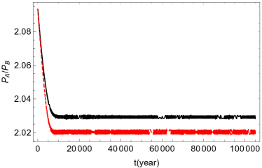
Figure 10: The evolution of a pair of planets with the same system parameters as in Fig. 9, except that the $\tau_{0}$ terms are turned on. For the red dashed line $\tau_{0}$ is set to be $-\tau_{nA}/20$ and for the black solid line $\tau_{0}$ is set to be $-\tau_{nA}/30$.

The multi-planet systems discovered that by the Kepler mission have shown interesting observational signatures (Fabrycky et al., 2014). First of all, most planets are found to reside away from mean-motion resonances. Secondly, for these found trapped in resonances, the period ratios are usually $1\%-2\%$ larger than the exact resonance. By introducing the damping terms in the eccentricity and semi-major axis, Goldreich & Schlichting (2014) manages to explain why it is rare to find planet-pairs trapped in resonances. However, their formalism suggests much smaller offsets (of period ratios) from the exact resonance for these pairs trapped in resonances.

In order to explain the period ratio offset, it was suggested that the tidal damping of eccentricity may play a role (Lithwick & Wu, 2012; Batygin & Morbidelli, 2013), although Lee et al. (2013) claims that tidal damping cannot account for the measured offsets with reasonable tidal parameters. On the other hand, the work by Podlewska-Gaca et al. (2012); Baruteau & Papaloizou (2013) suggests that the density waves from the companion damped around the planet may contribute to larger period ratios, which is possibly more efficient if a gap opens by the planet. In this section we investigate the effect coming from interfering density waves, without introducing extra dissipation mechanisms.

We extend the formalism discussed in Sec. 4 by including the dynamical evolution for both the inner and outer objects. The evolution equations are (we are dealing with a $2:1$ resonance) (Goldreich & Schlichting, 2014)

$$\dot{n}_{B} =1.89\mu_{A}n^{2}_{B}(1.19e_{B}\sin\phi_{B}-0.428e_{A}\sin\phi_{A})+\frac{n_{B}}{\tau_{nB}}+\frac{3n_{B}e^{2}_{B}}{\tau_{eB}}$$

$$-\frac{6e_{B}n_{B}\cos\phi_{B}}{\tau_{0}},$$

$$\dot{n}_{A} =-6\mu_{B}n^{2}_{A}(1.19e_{B}\sin\phi_{B}-0.428e_{A}\sin\phi_{A})+\frac{n_{A}}{\tau_{nA}}+\frac{3n_{A}e^{2}_{A}}{\tau_{eA}}\,,$$

$$\dot{e}_{B} =0.75\mu_{A}n_{B}\sin\phi_{B}-\frac{e_{B}}{\tau_{eB}}-\frac{\cos\phi_{B}}{\tau_{0}},$$

$$\dot{e}_{A} =-0.428\mu_{B}n_{A}\sin\phi_{A}-\frac{e_{A}}{\tau_{eA}},$$

$$\dot{\varpi}_{B} =-0.75\mu_{A}n_{B}\frac{\cos\phi_{B}}{e_{B}},$$

$$\dot{\varpi}_{A} =0.428\mu_{B}n_{A}\frac{\cos\phi_{A}}{e_{A}}$$ (64)

with $\phi_{A,B}:=\sigma-\varpi_{A,B}:=2\lambda_{A}-\lambda_{B}-\varpi_{A,B}$. Notice that in Eq. 5 we have only included the interfering density wave term $\tau_{0}$ for the evolution equations of object B for simplicity. This is a good approximation as later on we shall focus on the limit that $\mu_{A}\gg\mu_{B}$. In addition, the evolution equation for $\sigma$ is

$$\dot{\sigma}=2n_{A}-n_{B}\,,$$ (65)

which together with Eq. 5 provide seven evolution equations for seven variables $n_{A},n_{B},e_{A},e_{B},\varpi_{A},\varpi_{B},\sigma$. Let us now consider the case with $\mu_{A}\gg\mu_{B}$ discussed in Goldreich & Schlichting (2014). By setting $\mu_{B}=0,\mu_{A}=4\times 10^{-4}$ and $\tau_{eB}/\tau_{nA}=0.022$, the period ratio can reach a level $\sim 1.5\%$. However, most of the Kepler pairs near the $2:1$ resonance has $\mu_{A}$ being much smaller than $4\times 10^{-4}$, so that it was conjectured that additional eccentricity damping mechanism may be in operation.

In Fig. 9 we are presenting an evolution using Eq. 5 and Eq. 65 (but with $\tau_{0}$ terms removed) similar to Fig. $12$ of Goldreich & Schlichting (2014).The $\mu_{A}$ is assumed to be $10^{-4}$, which is a factor of four smaller than the value used in Goldreich & Schlichting (2014), and $\tau_{eB}$ is set to be $\tau_{nA/100}$. In the stationary state the system undergoes large amplitude librations, with the average period ratio offsets from $2$ by about $0.3\%$, which is clearly much smaller than $\it Kepler$ observations. This is consistent with the findings in Goldreich & Schlichting (2014), that $\mu_{A}$ has to be set with values higher than those observed in order to explain the $1\%-2\%$ period ratio offsets.

In Fig. 10 we present the evolution of planet pairs with in interfering density wave terms included. We find that with $\tau_{0}\sim-\tau_{nA}/30$ is the ratio offset can achieve the $1.5\%$ level without the requirement of increasing the mass $\mu_{A}$. This $\tau_{0}$ corresponds to

$$\frac{1}{|\tau_{0}\beta_{0}\mu^{\prime}n|}\approx 0.18\,,$$ (66)

so that the equivalent force coming from interfering density waves is about $20\%$ of the mutual gravitational interaction for the resonant dynamics. The quasi-stationary part of Fig. 10 can be understood as follows. This state is similar to the rotational state as depicted by the red and black trajectory in Fig. 5(b), although here the rotation amplitude is stationary due to the contribution from both $\tau_{0}$ and $\tau_{eB}$ related terms. If we follow the expansion in Eq. 4.1 for $n_{B}$ and $e_{B}$, we find that the unperturbed trajectory (without the $\tau_{eB},\tau_{nA},\tau_{0}$ terms) leads to

$$\delta n_{B} =-\frac{9\mu_{A}e_{B0}n^{2}_{B0}}{4\omega_{0}}\,,$$

$$\delta e_{B} =-\frac{3\mu_{A}n_{B0}}{4\omega_{0}}$$ (67)

where $\omega_{0}=2n_{A}-n_{B0}$. The corresponding conserved quantity $k$ for this system is given by

$$k=\frac{3e^{2}_{B}}{2}-\frac{3\mu_{A}\cos\phi_{B}}{4e_{B}}+\frac{\dot{Q}}{n_{B}}\,.$$ (68)

Now we treat the terms associated with $\tau_{0},\tau_{eB},\tau_{eA}$ as perturbations, and find that

$$\dot{k}=3e_{B}\dot{e}_{B}+\frac{2\dot{n}_{A}}{n_{B}}-\frac{\dot{n}_{B}}{n_{B}}=-\frac{6e^{2}_{B}}{\tau_{eB}}+\frac{3e_{B}\cos Q}{\tau_{0}}+\frac{1}{\tau_{nA}}\,.$$ (69)

The stationary state requires that the time average of $\dot{k}$ is zero, i.e., $\langle\dot{k}\rangle=0$, which leads to

$$\frac{1}{\tau_{nA}}-\frac{6e^{2}_{B0}}{\tau_{eB}}-\frac{9\mu_{A}n_{B0}}{4\tau_{0}\omega_{0}}\left(1+\frac{3n_{B0}e^{2}_{B0}}{2\omega_{0}}\right)=0\,.$$ (70)

Dropping the subdominant term in the bracket we obtain the period ratio offset as

$$\langle\frac{2n_{A}}{n_{B}}-1\rangle =\frac{\omega_{0}}{n_{B0}}\approx\frac{9\mu_{A}}{4}\frac{\tau_{nA}}{\tau_{0}}\left(1-\frac{6e^{2}_{B0}\tau_{nA}}{\tau_{eB}}\right)^{-1}$$ (71)

which is approximately $-1.5\%$ for $\tau_{0}=-\tau_{nA}/30$ (in the asymptotic state $e_{B0}\sim 0.03$), agreeing well with the numerical evolution. It is evident that strong torque from the interfering density waves would lead to larger period offset. It is also possible that the interfering density waves provide the eccentricity damping mechanism to allow large period ratio offsets as observed in Kepler multi-planet systems.

6 Conclusion

In this work we have discussed a new type of disc-mass interactions for a pair of point masses moving within an accretion disc. When the orbital phases of the masses are locked into a nearly constant resonant angle, the intefering density waves produce an extra piece of angular momentum flux that does not average to zero over orbital timescales. Using a two-dimensional theory with the same vertical averaging scheme in Ward (1988), we compute the backreaction of the disk on to the planets near a mean-motion resonance. We find that the backreaction torque is mainly contributed by the disk materials around the Lindbald resonance location close to one of the planets. The excitation amplitude $\Psi$ blows up for a standard two-dimensional theory but can be regularized by various smoothing schemes, e.g., the one discussed in Ward (1988). For the particular $2:1$ Inner resonance we find an overall positive torque acting on the inner planet due to this mechanism.

We have designed a set of hydrodynamical simulations to verify the analytical predictions. The simulations are also intrinsically two-dimensional, so that another smoothing scale $\epsilon$ is introduced in the gravitational potential following common practise in the literature of disk simulations. Interestingly, the analytical theory with this smoothing scheme predicts to a negative backreaction torque with a different magnitude. We perform a first simulation with a pair of planets evolving from a non-resonant state to a mean-motion resonant state, and measure the disk gravitational force onto the planets before and after the resonance capture. We also perform separate hydrodynamical simulations with either the outer planet or inner planet alone, but with orbital parameters the same as in the first simulation at the target times, and measure the disk backreaction. In this way we can subtract the torques and obtain the additional torque due to the coupling between the inner planet and the density waves generated by the outer planet. We find that indeed the additional torque is mainly produced in the Inner Lindblad resonance which is close to the orbit of the inner planet, with total value being $\sim-5.5\times 10^{-6}$ in code unit. Notice that the analytical theory using two smoothing schemes predicts a torque $\sim 10^{-6}$ (the same approach used in Ward (1988)) and $-2.5\times 10^{-6}$ (see Sec. 3), respectively . It is clear that the actual torque sensitively depends on the detailed three-dimension gas structure in the co-rotation regime of the inner planet. In the future, we plan to perform a study in the three-dimensional scenario both with the analytical theory and numerical simulations to resolve the discrepancy. Because the sign of the torque is not determined in this work, we have introduced an effective $\tau_{0}$ which can be both positive and negative (corresponding to positive and negative torques respectively) in the discussion of orbital dynamics in Sec. 4 and Sec. 5.

With the new torque due to density wave interference, we have analyzed the dynamics of a part of planets within and outside of the resonance regime. We find that positive $\tau_{0}$ tend to drive more systems into the resonance regime, whereas negative $\tau_{0}$ more likely drive the systems away from the resonant period ratios. Indeed in Kepler’s observation most planet pairs are found to be way from the resonant period ratios. Goldreich & Schlichting (2014) proposed an explanation by introducing dissipation terms in the orbital evolution equations but Deck & Batygin (2015) have pointed out that the model is insufficient to explain the data by considering more general mass ratios. It is therefore interesting to examine whether the interfering density wave effect can explain the large population of off-resonant pairs - an direction to explore in the future. On the other hand, we also find that negative $\tau_{0}$ can lead to a state with stable period ratio with $1\%-2\%$ offset away from the exact resonant values. This is another observation signatures of planet pairs in Kepler’s data which can not be naturally explained in Goldreich & Schlichting (2014). Here the interfering density waves provide an promising mechanism to produce relatively large period ratio offsets, but more extensive studies in the relevant parameter space are necessary to test whether it is fully consistent with data.

At this point, it may be interesting to generalize the effect due to interfering density waves to “resonant dissipations" for systems under resonance as density wave emission is one form of dissipation in a resonant process. The essence of this effect is that dissipative mechanisms may dynamically depend on the resonant angle, so that they may introduce nontrivial influence on the resonant dynamics. For example, one may imagine that the tide-driven migration in planet-satellite systems may exhibit similar phenomena. The planet tides excited by the satellites (Goldreich & Sciama, 1965) may coherently interfere with each other to produce additional resonant dissipation. In EMRI systems relevant for space-borne gravitational wave detection, with a single stellar-mass black hole orbiting around a massive black hole an orbital resonance may still arise because of the beating between different degrees of freedom of the orbit (Flanagan & Hinderer, 2012; Yang & Casals, 2017; Bonga et al., 2019; Pan et al., 2023), which have different cyclic frequencies in the strong-gravity regime. The main dissipation mechanism for these systems are gravitational wave radiation. The beating of gravitational waves of different harmonics near the resonance may give rise to an extra resonant dissipation that depends on the resonant angle and modify the resonant dynamics in a nontrivial manner.

Data availability

The data underlying this article will be shared on reasonable request to the corresponding author.

References

- Ansdell et al. (2016) Ansdell M., et al., 2016, The Astrophysical Journal, 828, 46
- Baruteau & Papaloizou (2013) Baruteau C., Papaloizou J. C. B., 2013, Astrophys. J., 778, 7
- Batygin & Morbidelli (2013) Batygin K., Morbidelli A., 2013, Astron. J., 145, 1
- Benítez-Llambay & Masset (2016) Benítez-Llambay P., Masset F. S., 2016, ApJS, 223, 11
- Bonga et al. (2019) Bonga B., Yang H., Hughes S. A., 2019, Phys. Rev. Lett., 123, 101103
- de Val-Borro et al. (2006) de Val-Borro M., et al., 2006, MNRAS, 370, 529
- Deck & Batygin (2015) Deck K. M., Batygin K., 2015, The Astrophysical Journal, 810, 119
- DeLaurentiis et al. (2023) DeLaurentiis S., Epstein-Martin M., Haiman Z., 2023, MNRAS, 523, 1126
- Dempsey et al. (2022) Dempsey A. M., Li H., Mishra B., Li S., 2022, ApJ, 940, 155
- Duffell & Chiang (2015) Duffell P. C., Chiang E., 2015, ApJ, 812, 94
- Fabrycky et al. (2014) Fabrycky D. C., et al., 2014, Astrophys. J., 790, 146
- Flanagan & Hinderer (2012) Flanagan E. E., Hinderer T., 2012, Phys. Rev. Lett., 109, 071102
- Goldreich & Schlichting (2014) Goldreich P., Schlichting H. E., 2014, Astron. J., 147, 32
- Goldreich & Sciama (1965) Goldreich P., Sciama D., 1965, Monthly Notices of the Royal Astronomical Society, 130, 159
- Goldreich & Tremaine (1979) Goldreich P. M., Tremaine S., 1979, Astrophys. J., 233, 857
- Goldreich & Tremaine (1980) Goldreich P., Tremaine S., 1980, Astrophys. J., 241, 425
- Kaaz et al. (2023) Kaaz N., Schrøder S. L., Andrews J. J., Antoni A., Ramirez-Ruiz E., 2023, ApJ, 944, 44
- Kocsis et al. (2011) Kocsis B., Yunes N., Loeb A., 2011, Phys. Rev. D, 84, 024032
- Lai & Muñoz (2023) Lai D., Muñoz D. J., 2023, ARA&A, 61, 517
- Lee et al. (2013) Lee M. H., Fabrycky D., Lin D. N. C., 2013, Astrophys. J., 774, 52
- Li & Lai (2022) Li R., Lai D., 2022, MNRAS, 517, 1602
- Li & Lai (2023) Li R., Lai D., 2023, MNRAS, 522, 1881
- Li et al. (2021) Li Y.-P., Dempsey A. M., Li S., Li H., Li J., 2021, ApJ, 911, 124
- Li et al. (2022) Li Y.-P., Dempsey A. M., Li H., Li S., Li J., 2022, ApJ, 928, L19
- Li et al. (2023) Li J., Dempsey A. M., Li H., Lai D., Li S., 2023, ApJ, 944, L42
- Lissauer et al. (2012) Lissauer J. J., et al., 2012, Astrophys. J., 750, 112
- Lithwick & Wu (2012) Lithwick Y., Wu Y., 2012, Astrophys. J. Lett., 756, L11
- Murray & Dermott (1999) Murray C. D., Dermott S. F., 1999, Solar system dynamics. Cambridge university press
- Murray & Dermott (2000) Murray C. D., Dermott S. F., 2000, Solar system dynamics. Cambridge university press
- Pan & Yang (2021a) Pan Z., Yang H., 2021a, Phys. Rev. D, 103, 103018
- Pan & Yang (2021b) Pan Z., Yang H., 2021b, Astrophys. J., 923, 173
- Pan et al. (2021) Pan Z., Lyu Z., Yang H., 2021, Phys. Rev. D, 104, 063007
- Pan et al. (2023) Pan Z., Yang H., Bernard L., Bonga B., 2023, arXiv e-prints, p. arXiv:2306.06576
- Peale (1976) Peale S. J., 1976, Ann. Rev. Astron. Astrophys., 14, 215
- Peng & Chen (2023) Peng P., Chen X., 2023, Astrophys. J., 950, 3
- Petrovich et al. (2013) Petrovich C., Malhotra R., Tremaine S., 2013, Astrophys. J., 770, 24
- Podlewska-Gaca et al. (2012) Podlewska-Gaca E., Papaloizou J. C. B., Szuszkiewicz E., 2012, Mon. Not. Roy. Astron. Soc., 421, 1736
- Rowan et al. (2023a) Rowan C., Whitehead H., Boekholt T., Kocsis B., Haiman Z., 2023a, arXiv e-prints, p. arXiv:2309.14433
- Rowan et al. (2023b) Rowan C., Boekholt T., Kocsis B., Haiman Z., 2023b, MNRAS, 524, 2770
- Shakura & Sunyaev (1973) Shakura N. I., Sunyaev R. A., 1973, A&A, 500, 33
- Tanaka & Ward (2004) Tanaka H., Ward W. R., 2004, The Astrophysical Journal, 602, 388
- Tanaka et al. (2002) Tanaka H., Takeuchi T., Ward W. R., 2002, The Astrophysical Journal, 565, 1257
- Wang et al. (2023) Wang Y., Zhu Z., Lin D. N. C., 2023, arXiv e-prints, p. arXiv:2308.09129
- Ward (1988) Ward W. R., 1988, Icarus, 73, 330
- Whitehead et al. (2023) Whitehead H., Rowan C., Boekholt T., Kocsis B., 2023, arXiv e-prints, p. arXiv:2309.11561
- Yang & Casals (2017) Yang H., Casals M., 2017, Phys. Rev. D, 96, 083015
- Yang et al. (2019) Yang H., Bonga B., Peng Z., Li G., 2019, Phys. Rev. D, 100, 124056