Breaking On-Chip Communication Anonymity using Flow Correlation Attacks

Abstract.

Network-on-Chip (NoC) is widely used to facilitate communication between components in sophisticated System-on-Chip (SoC) designs. Security of the on-chip communication is crucial because exploiting any vulnerability in shared NoC would be a goldmine for an attacker that puts the entire computing infrastructure at risk. NoC security relies on effective countermeasures against diverse attacks, including attacks on anonymity. We investigate the security strength of existing anonymous routing protocols in NoC architectures. Specifically, this paper makes two important contributions. We show that the existing anonymous routing is vulnerable to machine learning (ML) based flow correlation attacks on NoCs. We propose lightweight anonymous routing with traffic obfuscation techniques to defend against ML-based flow correlation attacks. Experimental studies using both real and synthetic traffic reveal that our proposed attack is successful against state-of-the-art anonymous routing in NoC architectures with high accuracy (up to 99%) for diverse traffic patterns, while our lightweight countermeasure can defend against ML-based attacks with minor hardware and performance overhead.

1. Introduction

Advanced manufacturing technology allows the integration of heterogeneous Intellectual Property (IP) cores on a single System-on-Chip (SoC). For example, Intel’s Xeon® Scalable Processor (Intel, 2023) supports up to 60 cores. Similarly, Altra® multicore server processor (Ampere, 2022) supports up to 192 cores. Traditional bus architectures fail to scale up with the communication requirements of the increasing number of IP cores. Network-on-Chip (NoC) is the preferred communication fabric to meet the high throughput and scalability requirements between these IP cores. Due to time to market constraints and cost-effectiveness, SoC manufacturers tend to use third-party vendors and services from the global supply chain (Mishra et al., 2021).

Typically only a few IP cores are designed in-house, while others are reusable IPs from third-party vendors. For example, FlexNoc interconnect is used by four out of the top five fabless companies to facilitate their on-chip communication (JS et al., 2015). A long and potentially untrusted supply chain can lead to the introduction of malicious implants through various avenues, such as untrusted CAD tools, rogue designers, or at the foundry. Furthermore, these sophisticated SoC designs make it harder to do complete security verification (Mishra et al., 2017). While the design of an energy-efficient NoC is the primary objective today, the security of the NoC is also crucial since exploiting NoC would be a goldmine for an attacker to access communication between various IP cores and compromise the security of the entire computing infrastructure.

Figure 1 shows a $4\times 4$ mesh NoC where mesh topology is the most commonly used topology in NoC. A single tile consists of an IP core, Network Interface (NI), and Router. Security issues in a typical NoC can be classified based on various security goals (confidentiality, integrity, anonymity, authenticity, availability, and freshness) compromised by an attacker (Weerasena and Mishra, 2023). There are efficient detection and mitigation of security vulnerabilities (Charles et al., 2020, 2021; Farahmandi et al., 2019; Lyu et al., 2020; Ahmed et al., 2018) for securing NoC-based SoCs. In a typical NoC, to enable fast packet forwarding, the header information is kept as plaintext while the packet data is encrypted. An adversary can implant a hardware Trojan in a router ($R_{8}$ in Figure 1), which can collect packets from the same source-destination pair and send them to a remote adversary that can launch traffic and metadata analysis attacks (Weerasena and Mishra, 2023). For example, imagine a source node ($IP_{S}$) is a cryptographic accelerator that needs to communicate with a memory controller, destination node ($IP_{D}$), to facilitate memory requests for the cryptographic operation. An adversary can use a malicious router in the middle to collect packets between $IP_{S}$ and $IP_{D}$ over a time interval and recover the key by launching a ciphertext-only cryptanalysis attack (Charles and Mishra, 2020; Sarihi et al., 2021). Furthermore, a collection of packets belonging to the same communication session can also be analyzed to discover what program is running at $IP_{S}$ or reverse engineer the architectural design using a simple hardware Trojan and powerful remote adversary (Ahmed et al., 2020, 2021; Dhavlle et al., 2023). Ensuring anonymity in NoC communication can mitigate metadata and traffic analysis attacks since anonymity ensures that there is no unauthorized disclosure of information about communicating parties. Recent literature features two anonymous routing approaches for securing NoC traffic: ArNoC (Charles et al., 2020), and a stochastic anonymous routing protocol (Sarihi et al., 2021). Even though these anonymous routing solutions provide packet-level anonymity, we show they fail to provide flow-level anonymity by breaking anonymity via flow correlation attacks. Specifically, this paper evaluates the security strength of anonymous routing protocols in NoCs and makes the following major contributions.

• We propose an attack on existing anonymous routing by correlating NoC traffic flows using machine learning.

• We demonstrate that the proposed machine learning (ML)-based attack can break the anonymity provided by the state-of-the-art anonymous routing (ARNoC (Charles et al., 2020) and  (Sarihi et al., 2021)) and validates the need for flow-level anonymity.

• The robustness of the proposed attack is evaluated across diverse configurations and traffic patterns.

• We propose a lightweight anonymous routing with traffic obfuscation that provides both packet-level and flow-level anonymity and defends against ML-based flow correlation attacks.

• Experimental results demonstrate that our countermeasure hinders flow correlation attacks’ effectiveness with minor hardware and performance overhead.

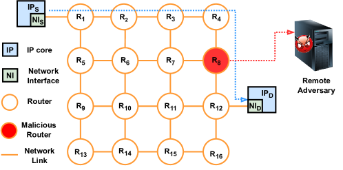
Figure 1. NoC with 4x4 mesh topology. Each IP is connected to NoC via a network interface followed by a router. A malicious router in the middle can collect packets when $IP_{S}$ communicates with $IP_{D}$ and send it to a remote adversary for sophisticated attacks.

The remainder of this paper is organized as follows. Section 2 provides relevant background and surveys the related efforts. Section 3 describes our ML-based attack on anonymous routing. Section 4 proposes a lightweight solution that can defend against ML-based attacks. Section 5 presents the experimental results and evaluation. Finally, the paper is concluded in Section 6.

2. Background and Related Work

This section provides the relevant background and surveys the related efforts to highlight the novelty of this work.

2.1. Network-on-Chip (NoC) Traffic

NoC enables communication by routing packets through a series of nodes. There are two types of packets that are injected into the network: control and data packets. Consider an example when a processor ($IP_{S}$) wants to load data from a particular memory controller ($IP_{D}$), it will issue a control packet requesting the data from memory. The packet will travel via routers based on a predefined routing protocol. Once the destination IP receives the control packet, it will reply with a data packet containing the requested data.

In general, header information is kept as plaintext and the payload data is encrypted. At each source NI, the packets are divided into fixed-size flits, which is the smallest unit used for flow control. There is a head flit followed by multiple body flits and tail flits. Routing in NoC can be either deterministic or adaptive; both approaches use header information to make routing decisions at each router. XY routing is the most commonly used routing in mesh-based traditional NoCs, which basically takes all the X links first, followed by Y links. NoC uses links to connect different components of the interconnects. Links can be either internal or boundary links. A boundary link refers to an outbound or inbound link that connects a router to a network interface, while internal links connect two routers. Our ML-based attack on anonymous routing makes use of the flow of flits (inter-flit delays), whereas our countermeasure manipulates routing decisions to create virtual tunnels.

2.2. Attacks on Anonymity and Anonymous Routing

In the context of communication, anonymity refers to the quality of being unidentifiable within a set of subjects. The primary goal of anonymity is to protect the privacy of communication parties. Traffic and metadata analysis are two types of attacks that compromise the lack of anonymity in NoC communication (Weerasena and Mishra, 2023). A traffic analysis attack collects packets in a particular communication session between parties and analyzes them to deduce various aspects, such as what type of application is running in an SoC. Similarly, metadata analysis attacks use ancillary data of communications, such as sender and receiver information, time stamps, and packet sizes, to compromise the privacy of communication parties. Anonymous routing hides the identity of the communicating parties from anyone listening in the middle and hinders the effectiveness of these attacks. In this context, we can consider two types of anonymity: packet-level and flow-level anonymity. Packet-level anonymity focuses on concealing individual data packets’ origin, destination, and content, while flow-level anonymity aims to obscure the relationship between packets in a communication session.

Tor network (Dingledine et al., 2004) (runs on top of onion routing) and I2P network (Zantout et al., 2011) (runs on top of garlic routing) are popular anonymous routing examples in traditional computer networks. Onion routing builds tunnels through a series of hops and the source applies layered encryption on the message where the number of hops equals to the number of layers, then encryption is peeled off at each hop to reveal the original message. Garlic routing is an extension of the onion routing where multiple messages are bundled and encrypted together, similar to garlic cloves. There are a wide variety of attacks to break the anonymity of the Tor network, including flow correlation attack (Nasr et al., 2018). This attack cannot be directly applied to NoC because of the following three reasons. (1) Traffic characteristics of NoC and traditional networks are significantly different because NoC uses its traffic primarily for cache coherence messages. (2) The existing attack relies heavily on packet size as a feature, whereas NoC flits are the fundamental unit of flow control, and they are of fixed size. (3) All NoC nodes act as onion routers, whereas in the traditional network, there is a mixture of both normal and onion routers.

2.3. Related Work

Anonymity is critical for secure on-chip communication; however, the solutions in the traditional networks are too expensive for resource-constrained NoCs.  Sarihi et al. (Sarihi et al., 2021) presented an anonymous routing that needs NoC packets to be identified as secure and non-secure packets. This approach stochastically selects a routing scenario for each packet out of three scenarios available and confuses adversaries. Charles et al. (Charles et al., 2020) presented an anonymous routing solution (ARNoC) for NoC based on onion routing (Dingledine et al., 2004) to ensure the anonymity of a communication session. ARNoC creates an on-demand anonymous tunnel from the source to the destination where intermediate nodes know only about the preceding and succeeding nodes. Our proposed ML-based attack can break the anonymity of both ARNoC and reference (Sarihi et al., 2021).

A threat model based on the insertion of Hardware Trojans (HTs) in network links is addressed in  (Yu et al., 2013; Boraten et al., 2016). Yu et al. (Yu et al., 2013) show that the Trojans can be inserted in boundary links and center links that can do bit flips in the header packet that can lead to deadlock, livelock, and packet loss.  Boraten et al. (Boraten et al., 2016) discuss the denial of service (DoS) attacks that can be launched by malicious links. This specific Trojan performs packet injection faults at the links, triggering re-transmissions from the error-correcting mechanism. (Ahmed et al., 2021) introduce the Remote Access Hardware Trojan (RAHT) concept, where a simple HT in NoC can leak sensitive information to an external adversary who can launch complex traffic analysis attacks. These RAHTs are hard to detect due to negligible area, power, and timing footprint. Our proposed attack also assumes malicious links at the points of data collection.  (Ahmed et al., 2021; Dhavlle et al., 2023) uses a similar threat model that can reverse engineer applications through traffic analysis.

ML-based techniques have been used to detect and mitigate attacks on NoCs in (Sudusinghe et al., 2021; Wang et al., 2020; Sinha et al., 2021). Sudusinghe et al. (Sudusinghe et al., 2021) used several ML techniques to detect DoS attacks on NoC traffic. Reinforcement learning is used by (Wang et al., 2020) to detect hardware Trojans in NoC at run time.  Sinha et al. (Sinha et al., 2021) use an ML-based approach to localize flooding-based DoS attacks. None of these approaches consider attacks or countermeasures related to anonymous routing in NoC architectures. To the best of our knowledge, our proposed ML-based flow correlation attack is the first attempt on breaking anonymity in NoC-based SoCs.

2.4. Flow Correlation Challenges

NoC traffic flow can be considered a time series data array with values of increasing timestamps in order. For example, in a communication session, we can consider an array of time differences between each packet coming into a node as a flow. Flow correlation is when we take two such pairs and compare if they are correlated in some manner. For example, in a network link, the flow of inter-flit delay entering and going out of the link are correlated. Though correlating outgoing and incoming traffic on a link seems straightforward, correlating traffic between two nodes in a large network with multiple hops in NoC is extremely difficult for the following reasons:

• The queuing delay at each hop is unpredictable and can interfere with traffic flow characteristics.

• A pair of correlated nodes may communicate with other nodes, which is considered as noise.

• The communication path of the correlated pair may be shared by other nodes in SoC, which will interfere with the traffic flow characteristics between correlated pairs.

3. ML-based Attack on Anonymous Routing

We first outline the threat model used in the proposed attack. Next, we describe our data collection, training, and application of the ML model to accomplish the attack.

3.1. Threat Model

The threat model considers an NoC that uses encrypted traffic and anonymous routing using ARNoC. Therefore, when we consider an individual packet, an attacker cannot recover the payload because it’s encrypted and cannot recover the sender/receiver identity because they are hidden via ARNoC. The threat model to break anonymity consists of three major components: (1) a malicious NoC, (2) a malicious program (collector), and (3) a pre-trained ML model.

Malicious NoC: The malicious NoC has malicious boundary links with Hardware Trojan (HT). The HT is capable of counting the number of cycles between flits (inter-flit-delay). Specifically, the HT can count inter-flit-delay of incoming and outgoing flits to/from an IP. After specific intervals, HT gathers all inter-flit delay into an array and sends it to the IP where the malicious program (collector) is running. HT can be inserted into an IP core by various adversaries in the extended supply chain, such as through untrusted CAD tools, rogue engineers, or at the foundry via reverse engineering, and remain undetected during post-silicon verification (Mishra et al., 2017). A similar threat model of inserting HT at NoC links has been discussed in (Yu et al., 2013; Boraten et al., 2016). Note that the area and power overhead of an HT with a small counter is negligible in a large MPSoC (Ahmed et al., 2020).

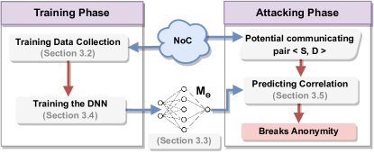
Figure 2. Overview of our proposed ML-based attack that consists of two phases (training and attacking).

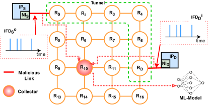
Figure 3. Malicious boundary links outside the anonymous tunnel extract flow pair ($IFD_{S}^{o}$, $IFD_{D}^{i}$) and send them to the collector. Then, collector sends them to ML-model.

Malicious Program: The collector is a malicious program, it activates/deactivates HT to keep it hidden from any run-time HT detection mechanisms. The main functionality of the collector is to collect inter-flit-delays from HT-infected links and send them to ML-model. Both the HT and collector must be within the same NoC-based SoC. This threat model, where a malicious NoC with an HT collaborates with a colluding application in same SoC ( i.e. collector), is a well-documented approach in NoC security literature (Weerasena and Mishra, 2023; Charles et al., 2021).

ML Model: The pre-trained ML model runs in a remote server/cloud controlled by the adversary. The flow correlation uses the attacking phase out of two phases (attacking and training) of the ML model. The attacking phase classify whether two inter-flit delay arrays are correlated or not. The training phase is discussed in detail in Section 3.4. Figure 2 shows a high-level overview of the proposed flow correlation attack categorized from the perspective of the ML model. The training phase is responsible for collecting data for training and conducting training of the ML model. The training is performed offline in the controlled environment (SoC or simulator mimicking the target SoC) owned by the adversary. The adversary can generate large amount of trained data by changing process mapping, benchmarks and other traffic characteristics (as discussed in Section 5.1) to make the model generic. While training the ML model for detecting correlation can be computationally expensive, it needs to be done only once and can subsequently be used for attacks throughout the lifetime of the SoC.

Figure 3 shows an example of the attacking phase on ARNoC. In ARNoC, a tunnel exists between source and destination routers if their associated IPs are in a communication session. ARNoC forms the tunnel to ensure anonymity by hiding the headers. The HTs in the links are in the inactive state by default. The collector periodically checks the state of all infected boundary links and flags communicating links as suspicious. This is done via monitoring a simple heuristic of inbound/outbound packet counts between two nodes. The collector will examine these counts and instruct the HT to start collecting inter-flit delays if the difference is within a specified threshold. Imagine a scenario where the adversary gets suspicious of the ongoing communication between the source ($IP_{S}$) and destination ($IP_{D}$); the collector activates HT associated with the boundary links of $IP_{S}$ and $IP_{D}$. On activation, HTs start sending periodic inter-flit delay arrays to the collector. More specifically, the Trojan will observe and leak both outbound ($IFD_{S}^{o}$) and inbound ($IFD_{D}^{i}$) traffic flows. Here, $IFD_{S}^{o}$ refers to the outbound inter-flit delay arrays from the source IP, and $IFD_{D}^{i}$ refers to the inbound inter-flit delay arrays at the destination IP. Upon receiving inter-flit delay arrays, the collector is responsible for sending collected data on inter-flit delay to the ML model. The adversary uses the ML model to pinpoint two specific nodes that are communicating and breaks the anonymity.

Breaking anonymity can have significant consequences in scenarios where preserving the anonymity of data traffic is critical. For example, in the case of confidential computing (Costan and Devadas, 2016), it can leak the host memory region of an application by breaking anonymity between the computing node and the memory controller. Furthermore, after breaking anonymity, an adversary can use already collected inter-flit delays to reverse-engineer applications running in the SoC (Ahmed et al., 2021) or use it as a stepping stone for more advanced attacks such as targeted denial-of-service attacks.

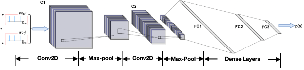
Figure 4. DNN architecture has two convolution layers (C1, C2) and three fully connected layers (FC1, FC2, FC3).

3.2. Collecting Data for Training

Algorithm 1 outlines the training data collection when running ARNoC. We collect inbound and outbound inter-flit delays for all source and destination IPs (line 4). Then, we label each flow pair as either ‘1’ or ‘0’ according to the ground truth (line 5). If $IP_{S}$ and $IP_{D}$ of flow pair $\{IFD_{S}^{o},IFD_{D}^{i}\}$ are correlated to each other ($IP_{S}$ and $IP_{D}$ communicating in a session), the flow pair is tagged as ‘1’ and otherwise ‘0’. These tagged flow pairs are utilized as the training set. Note that only the first $l$ elements of each flow of flow pair ($\{IFD_{S}^{o},IFD_{D}^{i}\}$) will be used in the training and testing. We consider the interference of external traffic (via shared path or shared resources) to correlated traffic flow characteristics by having other nodes communicating simultaneously with correlated pair communication. To evaluate the applicability of our model, we use a separate and unseen pair set during the testing phase. We utilize a deep neural network (DNN) as the ML model for our proposed flow correlation attack. In order to collect sufficient data to train DNN and make the dataset generic, we conduct multiple iterations of the data collection (Algorithm 1) by changing the mapping of correlated pairs to different NoC nodes each time. Section 5 elaborates on synthetic and real traffic data collection.

Algorithm 1 Data Collection

1:X, Y $\leftarrow\emptyset$

2:procedure CollectData ()

3:     for $\forall$ $(s,$ $d)$ $\in$ $(S$, $D)$ do

4:         $X$ $\leftarrow$ $X$ $\cup$ $\{$ $IFD_{s}^{o}$, $IFD_{d}^{i}$ $\}$

5:         $Y$ $\leftarrow$ $Y$ $\cup$ $c$ $\colon$ $c$ $\in$ $\{$ $0$, $1$ $\}$      

6:     return $X$, $Y$

3.3. DNN Architecture

We carefully examined various configurations and reached out to the final DNN architecture shown in Figure 4. We selected Convolution Neural Networks (CNN) (Schmidhuber, 2015) as our model architecture for the following reasons. First, since multivariate time series have the same 2-dimensional data structures as images, CNN for analyzing images is suitable for handling multivariate time series (Zhao et al., 2017). Second, recently published works using CNN for flow correlation (Guo et al., 2019; Nasr et al., 2018) has shown promising results. Inspired by existing efforts, our final architecture has two convolution layers followed by three fully connected layers to achieve promising performance. The first convolution layer (C1) has $k_{1}$ number of kernels of size (2, $w_{1}$). The second convolution layer (C2) has $k_{2}$ number of kernels of size (2, $w_{2}$). The main intuition of C1 is to identify and extract the relationship between two traffic flows ($IFD_{S}^{o}$, $IFD_{D}^{i}$), while we assign the task of advancing features to C2. In our approach, both C1 and C2 have a stride of (2, 1). A max-pooling layer immediately follows both convolution layers. Max pooling uses a max operation to reduce the dimension of features, which also logically reduces overfitting. Finally, the result of C2 is flattened and fed to a fully connected network with three layers. Additionally, the set ($k_{1}$, $k_{2}$, $w_{1}$, $w_{2}$) are considered as hyper-parameters. We provide details on hyper-parameter tuning in Section 5.2. We use ReLU as the activation function for all convolution and fully connected layers to avoid the vanishing gradient problem and improve performance. Due to the fact that our task is a binary classification, we apply a sigmoid function in the last output layer to produce predictions.

3.4. Training the DNN Model

Algorithm 2 outlines the major steps in the training process of the ML model. Specific sizes and parameters used in training are outlined in Section 5. We train the DNN for multiple epochs (line 6) for better performance of the model. We train the DNN by providing labeled inter-flit delay distributions. During the training phase, the stochastic gradient descent (sgd) optimizer minimizes the loss and updates the weights in the DNN (line 10). To achieve this binary classification results from the last fully connected layer pass through a sigmoid layer (Han and Moraga, 1995) (line 8) to produce classification labels.

Algorithm 2 ML Model Training

1:$X$ : [$x_{1}$, …, $x_{j}$, …, $x_{N}$] where $x_{j}=\{$ $IFD_{s}^{o}$, $IFD_{d}^{i}$ $\}_{j}$

2:$Y$ : [$y_{1}$, …, $y_{j}$, …, $y_{N}$] where $y_{j}\in\{0,1\}$

3:procedure TrainModel ($X$, $Y$)

4:     $Circuit$ $samples$ $X$ $and$ $labels$ $Y$

5:     $Model$ $M_{\Theta}$ $initialization$

6:     for $epoch$ $\in$ [$1$, …, $NoOfEpochs$] do

7:         for $x_{j}\in X$ and $y_{j}\in Y$ do

8:              $out_{j}$ = $sigmoid$( $M_{\Theta}(x_{j})$ )

9:              $loss$ = $\sum\limits^{N}_{j}$ cross_entropy$(out_{j},y_{j})$

10:              $\Theta$ = sgd($\Theta,\nabla loss$)               

11:     Return $M_{\Theta}$

Formally, the sigmoid layer is a normalized exponential function $f(x)=\frac{1}{1+e^{-x}}$, which aims at mapping the given vector to a probability value that lies in $[0,1]$. The value of the output of the last layer is the predicted label $p(y)$ which can be denoted as:

$$p(y)=\frac{1}{1+e^{-(M(s,d))}}\vspace{-0.1in}$$

where $s$ and $d$ denote the source and destination input distribution respectively, and $M$ denotes a function map for the entire DNN model.

Since it is a binary classification task, for given input $(s,d)$ pairs’ labels, their probability distributions are either $(1,0)$ for ‘true’ (correlated) and $(0,1)$ for ‘false’ (uncorrelated). Therefore, we choose binary cross-entropy (line 9) as the loss function as follows:

$$loss(p(y))=-\frac{1}{N}\sum\limits^{N}_{i=1}y_{i}\cdot log(p(y_{i}))+(1-y_{i})\cdot log(1-p(y_{i}))\vspace{-0.1in}$$

where $y$ is the label (1 for correlated pairs and 0 for uncorrelated pairs), and $N$ is the total number of training samples. The goal of model training is to minimize the loss function by gradient descent for multiple iterations, where in each step the model parameters $\Theta$ are updated by $\Theta^{\prime}=\Theta+\nabla loss(p(y))$.

3.5. Predicting Correlation

The trained model can be used for automatic correlation classification. The attacking phase is simple and straightforward as shown in Algorithm 3. During the attacking phase, we feed the two inter-flit delay arrays from a suspicious source ($S$) and destination ($D$) of the ongoing communication session to the ML model (lines 4-5). The ML model will output 1 if the source and destination are communicating, and 0 otherwise (lines 5). If $S$ and $D$ are communicating and the ML model output is 1, our attack has successfully broken the anonymity.

Algorithm 3 Attack on Anonymous Routing

1:$IFD_{S}^{o}$ : outbound inter-flit delay array of S

2:$IFD_{D}^{i}$ : inbound inter-flit delay array of D

3:$M_{\Theta}$ : pre-trained model

4:procedure Attack ( $\{IFD_{S}^{o},IFD_{D}^{i}\}$, $M_{\Theta}$)

5:     $p(y)$ $\leftarrow$ predict($\{IFD_{S}^{o},IFD_{D}^{i}\}$, $M_{\Theta}$)

6:     return $p(y)$

4. Defending against ML-based Attacks

In this section, we propose a lightweight anonymous routing that can defend against the ML-based attack described in Section 3. Figure 5 shows an overview of our proposed anonymous routing that consists of two phases: 1) outbound tunnel creation and 2) data transfer with traffic obfuscation. We utilize two traffic obfuscation techniques (chaffing of flits and random delays).

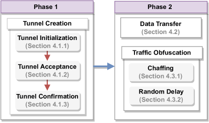
Figure 5. Overview of the proposed lightweight anonymous routing to defend against flow correlation attack. It has two phases: tunnel creation and data transfer with traffic obfuscation.

4.1. Outbound Tunnel Creation

An outbound tunnel ($OT^{i}_{S}$) is a route created from the source router ($S$) of the tunnel to an arbitrary router called tunnel endpoint ($E^{i}_{S}$). Here, $i$ indicates the parameter for each tunnel instance. Figure 6 shows how outbound tunnels, $OT_{S}^{i}$ and $OT_{D}^{i}$, are used when $IP_{S}$ and $IP_{D}$ are injecting packets to the network. It is important to highlight that these $OT^{i}$s are only bound to their source router and are independent of any communication session. Each tunnel is associated with a timeout bound. After the timeout, the tunnel that belongs to a particular source $S$ will cease to exist and a new tunnel will be created with a different endpoint ($E^{i+1}_{S}$). $E_{S}^{i}$ of an $OT_{S}^{i}$ is randomly selected from any router that is $h_{min}$ to $h_{max}$ hops away from the source of the tunnel. We use $h_{min}=3$ because a minimum of three nodes are needed for anonymous routing and increasing it further will negatively affect the performance (Dingledine et al., 2004). $h_{max}$ can be configured to balance the performance and the number of endpoint choices.

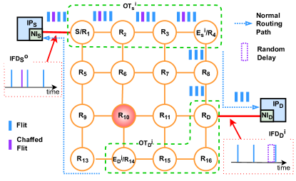
Figure 6. Two separate outbound tunnels $OT_{S}^{i}$ and $OT_{D}^{j}$ are used by $IP_{S}$ and $IP_{D}$ for communication. In $IP_{S}$ to $IP_{D}$ communication, chaffed flit is inserted at $NI_{S}$ and winnowed at $E^{i}_{S}$ ($R_{4}$). $E^{i}_{S}$ adds random delay to the flit sequence. The packet follows normal routing after an outbound tunnel ends.

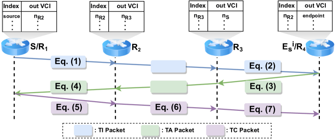
Figure 7. Message transfer in a three-way handshake to create an outbound tunnel between router $R_{1}$ and $R_{4}$ and final state routing tables of each router representing the outbound tunnel.

Figure 7 zooms into the tunnel creation phase. A summary of notations used in tunnel creation can be found in Table 1. Tunnel creation is a three-way handshake process. The source broadcasts a Tunnel Initialization (TI) packet to all the routers and only $E_{S}^{i}$ responds back to the source with a Tunnel Acceptance (TA) packet. Once the source receives an $ACK$ from $E_{S}^{i}$, it sends the Tunnel Confirmation (TC) packet to $E_{S}^{i}$. After these three steps, each router in the tunnel has two random Virtual Circuit Identifiers (VCI) saved in their routing table to define the succeeding and preceding hops representing the tunnel. For the rest of the section, we refer to $E^{i}_{S}$ as just $E$.

Table 1. Notations used in tunnel creation.

$E\hat{n}_{K}$	Encrypts message $M$ using key $K$
$D\hat{e}_{K}$	Decrypts message $M$ using key $K$
$OPuK_{S}^{i}$	One-time public key used by source $S$
$OPrK_{S}^{i}$	Corresponding private key to $OPuK_{S}^{i}$
$PuK_{E}$	Global public key of $E$
$PrK_{E}$	Corresponding private key to $PuK_{E}$
$TPuK_{R}^{i}$	Temporary public key of node $R$
$TPrK_{R}^{i}$	Corresponding private key to $TPuK_{R}^{i}$
$K_{S-R}$	Symmetric key shared between $S$ and $R$
$n_{R}$	Random nonce generated by node $R$
$r$	Random number generated by $S$
$pkt[i]$	$i^{th}$ element of a packet $pkt$
$pre(R)$	Previous router (in upstream direction)
$next(R)$	Next router (in downstream direction)
$rand(a,b)$	Generates random number between $a$ and $b$

4.1.1. Tunnel Initialization

In the example (Figure. 6), $S$ sends a TI packet as:

(1) $$\{TI||OPuK_{S}^{i}||E\hat{n}_{PuK_{E}}(OPuK_{S}^{i}||r)||TPuK_{S}^{i}\}\vspace{-0.1in}$$

$TI$ identifies the packet as a Tunnel Initiation packet. $OPuK_{S}^{i}$ is the sources’ one-time public key for the $i^{th}$ tunnel and $OPrK_{S}^{i}$ is the corresponding private key. In other words, an $OT^{i}_{S}$ can be uniquely identified by this key pair. $PuK_{E}$ and $PrK_{E}$ are the global public and private keys of $E$, respectively. They will not be changed with each tunnel creation. $OPuK_{S}^{i}$ and a randomly generated value $r$ is concatenated and encrypted through public-key encryption using the key $PuK_{E}$ ($E\hat{n}_{PuK_{E}}$). Only $E$ can decrypt this encryption because only E has the corresponding private key ($PrK_{E}$). Finally, the temporary public key ($TPuK_{S}^{i}$) is concatenated at the end of the packet. TI packet is broadcasted instead of directly routed to avoid anonymity being broken at its birth.

Algorithm 4 TI Packet handling at $R$

1:$pkt$ :A TI packet

2:procedure HandleTI ($pkt$)

3:     if  $OPuK_{S}^{i}$ in TL table then

4:         discard $pkt$

5:     else

6:         store $OPuK_{S}^{i}$ and $TPuK_{pre(R)}^{i}$      

7:     if  $D\hat{e}_{PrK_{R}}(pkt[3])$ is successful then

8:         GenerateTA ($D\hat{e}_{PrK_{R}}(pkt[3])$, $pkt[4]$)

9:     else

10:         $pkt[4]\leftarrow TPuK_{R}^{i}$

11:         forward $pkt$      

Any Router ($R$) receiving a TI packet will follow Algorithm 4. Tunnel Lookup (TL) table has unique entries for every TI packet comes to the router. First, it tries to match $OPuK_{S}^{i}$ with the existing entries in the TL table. On match, the message will get discarded to avoid any duplication due to TI packet broadcasting (line 4). Otherwise, $OPuK_{S}^{i}$ and $TPuK_{pre(R)}^{i}$ are stored in the TL table (line 6). Next, $R$ will try to decrypt the message and if it is successful, it should recognize itself as the intended endpoint and run Algorithm 5 (line 8). If not, $R$ will replace $TPuK_{pre(R)}^{i}$ with its own temporary key $TPuK_{R}^{i}$ and forward the TI packet to the next hop ($next(R)$)(line 10 and 11). For example, in figure 6, after receiving a TI packet from $R_{2}$, $R_{3}$ will generate and forward the following TI packet to $R_{4}$:

(2) $$\{TI||OPuK_{S}^{i}||E\hat{n}_{PuK_{E}}(OPuK_{S}^{i}||r)||TPuK_{R_{3}}^{i}\}\vspace{-0.1in}$$

4.1.2. Tunnel Acceptance

Algorithm 5 TA packet generation at $E$

1:$parm_{1}$ : parameter resolved to $OPuK_{S}^{i}||r$

2:procedure GenerateTA ($in_{1}$, $TPuK_{R}$)

3:     if $parm_{1}[1]\neq OPuK_{S}^{i}$  then

4:         discard the $pkt$

5:     else

6:         generate and store $n_{E}$ and $K_{S-E}$

7:         $enc\leftarrow E\hat{n}_{TPK_{next(E)}^{i}}(E\hat{n}_{OPuK_{S}^{i}}(r||n_{E}||$ $K_{S-E}))$

8:         return $\{TA||enc\}$      

Upon receiving the TI packet, $E$ runs Algorithm 4 first and then calls Algorithm 5 as the endpoint of the tunnel. Algorithm 5 shows the outline of TA packet generation at any endpoint router ($E$). First, $E$ validates the integrity of the packet by comparing decrypted $OPuK_{S}^{i}$ value and plaintext $OPuK_{S}^{i}$ value (line 3). If the packet is validated for integrity, Algorithm 5 will execute the following steps. First, it will generate random nonce $n_{E}$ which will be used as VCI. Next, it will generate a symmetric key $K_{S-E}$ to use between $S$ and $E$. Then it will log both $n_{E}$ and $K_{S-E}$ in the TL table and $n_{E}$ in the routing table as indexed VCI (line 6). Next, it will perform encryption of the concatenation of $n_{E}$, $K_{S-E}$ and $r$ using the key $OPuK_{S}^{i}$ which will allow only $S$ to decrypt the content (line 7). Finally, the resultant encryption is encrypted again by the $TPuK_{next(E)}$ (line 7). In the figure 6, $E^{i}_{S}$ will generate the following TA packet:

(3) $$\{TA||E\hat{n}_{TPuK_{R_{3}}^{i}}(E\hat{n}_{OPuK_{S}^{i}}(r||n_{E}||K_{S-E}))\}$$

Algorithm 6 TA packet handling at R

1:$pkt$ : A TA packet

2:procedure HandleTA ($pkt$)

3:     if  $R$ is $S$ of $OT^{i}$ then

4:         GenerateTC ($pkt$)

5:     else

6:         $dct\leftarrow D\hat{e}_{TPrK_{R}^{i}}(pkt[2])$

7:         generate and store $n_{R}$ and $K_{S-R}$

8:         $enc\leftarrow E\hat{n}_{OPuK_{S}^{i}}(dct||n_{R}||K_{S-R})$

9:         $enc\leftarrow E\hat{n}_{TPuK_{next(R)}^{i}}(enc)$

10:         return $\{TA||enc\}$      

When a router $R$ receives a TA packet, it will execute Algorithm 6. If the router is the source of the $OT^{i}$, it will execute Algorithm 7 (line 4). Otherwise, it will go through the following steps. First, it decrypts the packet using the temporary private key ($TPrK_{R}^{i}$) (line 6) and generates a random nonce and symmetric key ($n_{R}$, $K_{S-R}$). This generated $n_{R}$ and $K_{S-R}$ are stored in $R$’s TL table (line 7). The nonce and symmetric key pair is concatenated to the decrypted packet ($dct$) (line 7 and 8), which will be encrypted using source public key ($OPuK_{S}^{i}$) to add another layer of security (line 8). Finally, $R$ will encrypt the content with the public key of the next hop $next(R)$ (line 9). In the example, $R_{2}$ forwards the following TA packet to $R_{1}$:

(4) $$\{TA||E\hat{n}_{TPuK_{R_{2}}^{i}}(E\hat{n}_{OPuK_{S}^{i}}(E\hat{n}_{OPuK_{S}^{i}}(E\hat{n}_{OPuK_{S}^{i}}(r||n_{E}||K_{S-E})||n_{R_{3}}||K_{S-R_{3}})||n_{R_{2}}||K_{S-R_{2}}))\}$$

Algorithm 7 TC packet generation at S

1:$pkt$ :A TA packet

2:procedure GenerateTC ($pkt$)

3:     $dec\leftarrow D\hat{e}_{TPrK_{S}^{i}}(pkt[2])$

4:     for no of hops in OT do

5:         $dec\leftarrow D\hat{e}_{OPrK_{S}^{i}}(dec)$      

6:     $enc\leftarrow r$

7:     for R = E to next(S) do

8:         $enc\leftarrow n(R)||E\hat{n}_{K_{S-R}}(enc)$      

9:     return $\{TC||enc\}$

4.1.3. Tunnel Confirmation

Algorithm 7 depicts the TC packet generation at the source router $S$. $TPrK_{S}^{i}$ is used to decrypt the outermost encryption (line 3), then each layer of the inner encryption is peeled away using the $OPrK_{S}^{i}$ (loop from line 4 to 5). $S$ extracts information of all the VCIs and symmetric keys. $r$ is used to check the authenticity of the packet received (make sure the TA is a packet from the actual endpoint $E$). Finally, starting from $E$ to $pre(S)$ (reverse order of routers in tunnel excluding $S$), $r$ is encrypted by the respective symmetric key and concatenated with the respective nonce iteratively (loop from line 7 to 8). In the figure 6, $S$ generates the TC packet structured as:

(5) $$\{TC||n_{R_{2}}||E\hat{n}_{K_{S-R_{2}}}(n_{R_{3}}||E\hat{n}_{K_{S-R_{3}}}(n_{E}||E\hat{n}_{K_{S-E}}(r)))\}$$

$TC$ denotes the packet type. The packet is layered and encrypted using the symmetric keys distributed in the previous stage. Here, $n_{*}$ represents the outgoing VCI at each router from $S$ to $prev(E)$. For example, $n_{R_{2}}$ defines outgoing VCI of $S$ and $n_{R_{3}}$ defines outgoing VCI for $R_{2}$. After the TC packet is received by each node, it decrypts the outermost layer and stores the corresponding outgoing VCI value in the routing table indexed as incoming VCI. For example, when $R_{2}$ receives the packet it will decrypt the content using key $K_{S-R_{2}}$ and store the outgoing VCI as $n_{R_{3}}$ in the routing table indexed as $n_{R_{2}}$. Similarly, all the routers in between $S$ and $E$ will update the routing table entry corresponding to the tunnel. In the example, $R_{2}$ will send $TC$ packet to $R_{3}$ structured as follows:

(6) $$\{TC||n_{R_{3}}||E\hat{n}_{K_{S-R_{3}}}(n_{E}||E\hat{n}_{K_{S-E}}(r))\}$$

Finally, $R_{3}$ will send the TC packet to $E$ ($R_{4}$) structured as:

(7) $$\{TC||(n_{E}||E\hat{n}_{K_{S-E}}(r)\}$$

The packet transfers during the tunnel creation is inherently secure. This is because the tunnel creation phase ensures the transfer of only publicly available information as plaintext, while all sensitive data (including VCIs) are encrypted using symmetric or asymmetric methods. The only way an attacker can break anonymity of a packet is by knowing all the VCIs of the tunnel. This is not possible since the asymmetric and symmetric cryptography are computationally secure.

4.2. Data Transfer

A previously created outbound tunnel ($OT_{S}^{i}$) is used to transfer messages anonymously from $IP_{S}$ to $IP_{D}$. Before transferring the packet, the source will encrypt the actual destination header using the key $K_{S-E}$ which is the symmetric key shared between the source and endpoint during the tunnel creation. When we consider the data transfer through tunnel $OT_{S}^{i}$, a Data Transfer (DT) packet is injected into the tunnel by S structured as:

$\{DT||n_{R_{2}}||E\hat{n}_{K_{S-E}}(D)||E\hat{n}_{D}(M)\}$

Here, DT is the packet type identifier, $n_{R_{2}}$ is the outgoing VCI, and $E\hat{n}_{D}(M)$ is the encrypted payload of the packet. At the router, $R_{2}$, the outgoing VCI is identified through a simple routing table lookup on the incoming VCI of the packet. Then $R_{2}$ replaces the outgoing VCI of the packet ($n_{R_{2}}$) with the next outgoing VCI, which is $n_{R_{3}}$, and routes the packet to the next hop. Similarly, $R_{3}$ replaces the outgoing VCI of the packet to $n_{E}$. Note that any intermediate node including $E$ does not know both source and destination of a single packet which ensures anonymity.

4.3. Traffic Obfuscation

We introduce traffic obfuscation techniques to hinder ML-based flow correlation. The main intuition behind the flow obfuscation is to add noise to inbound and outbound flows ($IFD_{S}^{o}$, $IFD_{D}^{i}$), so it will be harder for ML-model to do accurate flow correlation. Section 4.3.1 and 4.3.2 introduce two traffic obfuscation techniques.

4.3.1. Obfuscation with Chaffs

We introduce a chaffing scheme as our first obfuscation technique. Chaff is a dummy flit with no usable data. Specifically, we insert chaff/chaffs in outbound tunnel traffic at the network interface of the source and filter out chaffs at the endpoint of the tunnel. The outbound flow ($IFD_{S}^{o}$) will have inter-flit delay data relevant to both chaffs and legitimate flits but inbound flow ($IFD_{D}^{i}$) will have inter-flit delay data relevant only to legitimate flits. Algorithm 8 describes the chaffing process at the NI of the source. Wakeup procedure (Line 1 - 4) is the periodical function called by every NI in every clock cycle. We introduce a procedure named AddChaff (Line 5 - 23) to obfuscate traffic through chaffing.

We insert chaffs in two specific scenarios to ensure the obfuscation scheme works with the majority of traffic patterns: (i) first scenario: insert chaffs in the long gap between flits (line 6 - 13), and (ii) second scenario: insert chaff flit in middle of closely packed flits (line 14 - 21). When the outbound link of source NI is idle for more than $T_{c}$ cycles (Line 6, the first scenario is considered. The intuition behind this method is to hinder the possibility of ML-model using long inter-flit delays of inbound and outbound flows in sparse traffic scenarios. In order to control overhead, we use a percentage threshold ($P_{c}$) and ensure only $P_{c}$ of idle gaps between packets get obfuscated (line 8 - 9). If chosen to be obfuscated, a dummy packet of is created and is enqueued to the output queue of the NI (line 10 - 13). At the endpoint of the tunnel, the dummy flits are filtered out and discarded. The chaffId header is used to identify chaffed flit or packet. In the first scenario, a hash of the NI identification number is used as chaffed id. Unlike other headers, this header is encrypted by $K_{S-E}$ which is the symmetric key shared between the source ($S$) and endpoint ($E$) during the tunnel creation (line 12). Therefore, only endpoint can filter chaffed packets by decrypting $E\hat{n}_{K_{S-E}}$(hash($NI_{ID}$).

When the input queue of source NI received a packet (line 14), the first scenario is considered (line 15 - 21). The intuition behind this scenario is to hinder the possibility of ML-model using burst of small inter flits delays of inbound and outbound flows in heavy traffic. The example shown in Figure 6 demonstrates the chaffing in second scenario and removing that chaff. Here, $P_{c}$ limits the number of packets being obfuscated (line 16 - 17). If chosen to be obfuscated, chaff is inserted in the middle of legitimate packets at a random position (Line 18 - 21). $K_{S-E}$ is used to encrypt chaffId, represents the position of chaff flit, which is used by the endpoint to filter the chaffed flit.

A random number generator is already in the NI for cryptographic process. Therefore, the same generator is used for random number generation in line 8, 10 and 16. If the cflag (line 3, 6, 7, 15 and 23) variable is true, it indicates the current gap between flits was already checked for insertion of packet. It is important to note that, (1) the dummy flits are added only when outbound link is idle, therefore, it has less impact on the program running on source IP, and (2) the dummy flits will only impact at most 3 internal links associated with the tunnel, therefore, it has less impact on the other traffic in the network. The scenario two inserts relatively less number of dummy flits and they will only impact at most 3 internal links. Experimental results in Section 5.8 validate that our obfuscation technique only results in negligible overhead.

Algorithm 8 Add Chaff at source NI

1:procedure Wakeup ( )

2:     …..

3:     AddChaff($cflag$)

4:     …..

5:procedure AddChaff($cflag$)

6:     if  $cflag$ = $False$ and getIdleCy($link_{o}$) $>T_{c}$ then

7:         $cflag$ = True

8:         $randNo$ $\leftarrow$ $rand(0,99)$

9:         if  $randNo$ $\leq P_{c}$  then

10:              $nFlits$ $\leftarrow$ $rand(4,5)$

11:              $dPkt$ $\leftarrow$ $new$ $Packet(nFlits)$

12:              $dPkt.chId$ $\leftarrow E\hat{n}_{K_{S-E}}(hash(NI_{ID})$)

13:              $outputQueue.enque(dummyPkt)$               

14:     if $inputQueue.recivedPacket()$ = $True$  then

15:         $cflag$ = True

16:         $randNo$ $\leftarrow$ $rand(0,99)$

17:         if  $randNo$ $\leq P_{c}$  then

18:              $chId$ $\leftarrow$ $rand(0,len(inputPkt))$

19:              $dFlit$ = $new$ $flit()$

20:              $encChId$ $\leftarrow E\hat{n}_{K_{S-E}}(hash(NI_{ID})|chId$)

21:              $pkt.insert(chId,encChId,dFlit)$               

22:     if $outputQueue.sendPacket()$ = $True$  then

23:         $cflag$ = $False$      

4.3.2. Obfuscation with Random Delay

The second obfuscation technique adds random delays to selected flits and tries to tamper with the timing aspect of the traffic flow. Flits belonging to only $P_{d}$ percentage of packets are subject to added delays. The tunnel endpoint is responsible for adding delays. Traveling through the rest of the hops the flit propagates the delay to the destination tampering with timing features of the inbound flow ($IFD_{D}^{i}$). Figure 6 demonstrates the effect of added delay in traffic flows. It is clear that chaffing and random delays obfuscate the actual traffic between source and destination. Both of these techniques can be used simultaneously or in a standalone manner depending on the requirement. Experimental results (Table 11 and 12) demonstrate that both of these techniques are beneficial in defending against ML-based flow correlation attacks.

5. Experimental Evaluation

Table 2. System and interconnect configuration

Parameter	Details
Processor configurations	X86, 2GHz
Coherency Protocol	MI
Topology	8$\times$8 Mesh
Chaffing rate ($P_{c}$)	50%
Delay addition rate ($P_{d}$)	50%

We model our proposed ML-based attack and countermeasures on a cycle-accurate Gem5 (Binkert et al., 2011), a multi-core simulator, with Garnet 2.0 (Agarwal et al., 2009) for the interconnection network modeling. We use 64-core system with multiple and the detailed system configuration is given in Table 2. Splash-2 (Sakalis et al., 2016) benchmark applications as well as multiple synthetic traffic patterns were used in evaluation. We used Pytorch library to implement the proposed DNN architecture. In order to evaluate the area and energy overhead of our approach against ARNoC, we implemented them in Verilog and synthesized both designs (ARNoC and our approach) using Synopsys Design Compiler with 32nm Synopsys standard cell library. First, we show the results of the flow correlation attack in ARNoC (Charles et al., 2020). Later, we show the robustness of the proposed countermeasure to prevent the attack.

5.1. Data Collection

This section demonstrates the data collection on Gem5 for the training of DNN. Although the input to DNN is in the same structure, the inherent differences in synthetic traffic and real benchmarks led us to two ways of collecting flow pairs for training.

5.1.1. Synthetic Traffic

We performed data collection using Uniform-Random synthetic traffic with the following modification. All IPs send packets to randomly selected IPs except two ($IP_{S}$ and $IP_{D}$). These two IPs are the correlated pair communicating in a session. From all the packets injected from the source IP ($IP_{S}$), only $p$ percent of packets are sent to the destination IP ($IP_{D}$), and the remaining packets ($(100-p)$%) are sent to other nodes. For example, $p=80\%$ means 80% of the total outbound packets from $IP_{S}$ will have $IP_{D}$ as the destination, while the other 20% can have any other IP except IP $IP_{S}$ and $IP_{D}$ as the destination. Note that this 20% can be viewed as noise from the perspective of communication between $IP_{S}$ and $IP_{D}$. Here, traffic between correlated pair models concentrated point-to-point traffic between two nodes (e.g., processing core and memory controller). The random point-to-point traffic models other NoC traffic in a heterogeneous SoC other than cache coherence traffic such as monitoring and management traffic, inter-process communication and message passing between heterogeneous IP cores. This randomized traffic between uncorrelated pairs introduces uncontrolled noise to correlated traffic flow. Therefore, random point-to-point synthetic traffic models worst-case-scenario for flow correlation attack.

To make the dataset generic, for a single $p$ value, we conduct experiments covering all possible mapping of correlated pairs to NoC nodes, which are 8064 mappings (64$\times$63$\times$2). We consider four traffic distributions with $p$ value of 95%, 90%, 85%, and 80%. In other words, we consider four different noise levels (5%, 10%, 15% and 20%) for our data collection simulations. The full dataset for a certain $p$ value contains 24192 flow pairs ({$IFD_{S}^{o}$, $IFD_{D}^{i}$}) which consists of 8064 correlated traffic flow pairs and 16128 uncorrelated traffic flow pairs. Note that for each correlated flow pair, we selected two arbitrary uncorrelated flow pairs. To evaluate our countermeasures, when collecting obfuscated traffic, we kept both $P_{c}$ and $P_{d}$ at 50% to ensure uniform distribution of obfuscation. When obfuscating traffic using added delay, we vary the delay between $1-5$ cycles because a higher delay may lead to unacceptable performance overhead. We collected three categories of data sets: one with chaffing only, one with random delay only, and one with applying both chaffing and delaying simultaneously.

5.1.2. Real Traffic

Here, we collect response cache coherence traffic from memory controller to requester. This is done via filtering out using virtual network (vnet) used for memory response traffic to requester which is vnet 4. We consider five Splash-2 benchmark application pairs running on two processors ($P_{1}$ and $P_{2}$) where two memory controllers ($MC_{1}$ and $MC_{2}$) are serving memory requests. The benchmark pairs used are {fft, fmm}, {fmm, lu}, {lu, barnes}, {barnes, radix}, {radix, fft}, where the first benchmark runs on $P_{1}$ and the second runs on $P_{2}$. The selected benchmarks have the diversity to make the dataset generic (for example, fft and radix are significantly different  (Bienia et al., 2008)). The address space of the benchmark running in $P_{1}$ is mapped only to $MC_{1}$. Therefore, $P_{1}$ only talks with the $MC_{1}$, and they are the correlated pair. The address space of the benchmark running in $P_{2}$ is assigned to both $MC_{1}$ and $MC_{2}$ in a way that, the ratio between memory request received by $MC_{1}$ from $P_{1}$ to memory request received by $MC_{1}$ from $P_{2}$ to be $p:(100-p)$. This percentage $p$ is similar to that of synthetic traffic and $(100-p)\%$ is the noise. For example, when $p=85\%$, $MC_{1}$ serves $15\%$ packets to $P_{2}$ when it severs $85\%$ packets to $P_{1}$.

Similar to synthetic traffic, we considered four values for $p$ which are 95%, 90%, 85%, and 80%. For a single $p$ value and a single benchmark pair, we conducted experiments covering all possible mapping of correlated pairs to NoC nodes, which are 4032 mappings (64$\times$63). The $MC_{2}$ and $P_{2}$ were randomly chosen in all these mappings. The full dataset for a certain $p$ value and benchmark pair contains 16128 flow pairs (4032 correlated pairs and 12096 uncorrelated pairs). To evaluate our countermeasures, we collect obfuscated data similar to synthetic traffic.

5.2. Hyperparameter Tuning

Hyperparameters are the components fixed by the user before the actual training of the model begins to achieve the highest possible accuracy on the given dataset. We exhaustively tested different combinations of hyperparameters to attain state-of-the-art performance on attacking success rate. The training process consists of 10 epochs with a consistent learning rate of 0.0001. We performed batch normalization and adjusted the batch size to 10 for the training set. As for convolution layers (C1 and C2 in Figure 4), the channel size is selected as $k_{1}=1000$ and $k_{2}=2000$, with $w_{1}=5$ and $w_{2}=30$, for C1 and C2, respectively. As for fully connected layers, sizes are selected as 3000, 800, and 100 for FC1, FC2, and FC3, respectively.

There are a lot of challenges in tuning since the finalized parameters reflect a trade-off between cost and effectiveness. First, the learning rate of the raining was reduced from 0.001 to 0.0001 which increases the training time but successfully avoids the Local Minima problem. Also, we halve the training epochs from 20 to 10 to evade the Overfitting problem. Batch size is also decreased from 50 to 10. In this way, fewer samples are provided for one iteration of training, but it improves the stability of training progress. Additionally, the selection of parameters for convolution layers properly addressed their responsibilities. As discussed in Section 3.3, C1 focuses on extracting rough relationships while C2 on advancing features. Therefore, C2 possesses two times of channels of C1, and a wider stride (30:5) to improve efficiency.

5.3. Training and Testing

In our work, a total dataset of flow pairs for a certain configuration was randomly split in a proportion of 2:1 for training and testing set. The correlated flow pairs were labeled as ‘1’ and the uncorrelated pair as ‘0’. We use the following four evaluation metrics for our experimental evaluation.

Accuracy: $$\frac{tp+tn}{tp+tn+fp+fn} \frac{tp}{tp+fn} \frac{tp}{tp+fp} 2\frac{\text{Precision}\cdot\text{Recall}}{\text{Precision}+\text{Recall}}$$ Recall: Precision: F1 Score:

Here, $tp$, $tn$, $fp$ and $fn$ represent true positive, true negative, false positive, and false negative, respectively. Intuitively, recall is a measure of a classifier’s exactness, while precision is a measure of a classifier’s completeness, and F1 score is the harmonic mean of recall and precision. The reason for utilizing these metrics comes from the limitation of accuracy. For imbalanced test cases (e.g., $>90\%$ positive labels), a naive ML model which gives always-true output can reach $>90\%$ accuracy. The goal of the attacker is to identify correlating node pairs and launch complex attacks. Here, $fn$ is when an actual correlating pair is tagged as non-correlating by the DNN. $fp$ is when an actual non-correlating pair is tagged as correlating by the DNN. From an attacker’s perspective, the negative impact of wasting time on launching an unsuccessful attack on $fp$ is relatively low compared to an attacker missing a chance to launch an attack due to a $fn$. Therefore, recall is the most critical metric compared to others when evaluating this flow correlation attack.

5.4. ML-based Attack on Synthetic Traffic

We evaluated the proposed attack for all four traffic distributions. The traffic injection rate was fixed to 0.01 and the IFD array size to 250. Table 3 summarizes the results for the attack. All the considered traffic distributions show good metric numbers. We can see a minor reduction in performance with a reducing value of $p$. This is expected because of the increase in the number of uncorrelated packets in correlated flow pairs, making the correlation hard to detect. Even for the lowest traffic distribution of 80% between two correlating pairs, the attacking DNN is able to identify correlated and uncorrelated flow pairs successfully with good metric values. This confirms that our attack is realistic and can be applied on state-of-the-art anonymous routing (ARNoC) to break anonymity across different traffic characteristics with varying noise.

Table 3. Performance of ML-based attack on existing anonymous routing (ARNoC (Charles et al., 2020)) for different traffic distributions.

$p$	Accuracy	Recall	Precision	F1 Score
95	97.16%	91.98%	99.47%	95.58%
90	97.04%	93.35%	97.50%	95.38%
85	94.64%	91.32%	92.30%	91.81%
80	91.70%	80.02%	94.10%	86.60%

5.5. Stability of ML-based Attack

In this section, we evaluate the attack with varying configurable parameters to further confirm the stability of the proposed ML-based attack. For experiments in this section, we use synthetic traffic with the value of $p$ as 85% and the rest of the parameters as discussed in the experimental setup except for the varying parameter.

5.5.1. Varying traffic injection rates (TIR)

We collected traffic data for four traffic injection rates: 0.001, 0.005, 0.01 and 0.05, and conducted the attack on existing anonymous routing. Table 4 provides detailed results on metrics over selected values. We can see a small reduction in overall metrics including recall, with the increase in injection rate. This is because, higher injection rates will create more congestion and buffering delays on NoC traffic. The indirect noise from congestion and buffering delays makes it slightly hard for the ML model to do flow correlation. Overall, our proposed ML model performs well in different injection rates since all the metrics show good performance.

Table 4. Performance of ML-based attack on existing anonymous routing for different traffic injection rates.

TIR	Accuracy	Recall	Precision	F1 Score
0.001	95.32%	92.29%	93.51%	92.89%
0.005	94.72%	90.14%	93.98%	92.02%
0.01	94.64%	91.32%	92.30%	91.81%
0.05	93.86%	88.56%	92.67%	90.56%

5.5.2. Varying IFD Array Size

We collected traffic data by varying the size of IFD array size ($l$) in the range of 50 to 550 and conducted the attack on existing anonymous routing. Table 5 shows detailed results on metrics over selected values. For a lower number of flits, the relative values of the recall and other metrics are low. However, with the increasing number of flits, the accuracy also improves until the length is 250. This is due to the increase in the length of the IFD array the ML model has more features for the flow correlation. After the value of 250, the accuracy saturates at around 94.5%. In subsequent experiments, we kept $l$ to 250 because ML-based attack performs relatively well with less monitoring time.

Table 5. Performance metrics of ML-based attack on existing anonymous routing for varying number of flits.

IFD Array size(l)	Accuracy	Recall	Precision	F1 Score
50	83.53%	96.45%	67.96%	79.74%
100	90.92%	96.17%	80.28%	87.51%
150	90.93%	74.10%	98.32%	84.51%
250	94.64%	91.32%	92.30%	91.81%
350	94.71%	86.21%	97.39%	91.46%
450	94.58%	93.21%	90.58%	91.87%
550	94.66%	88.97%	94.30%	91.56%

Table 6. Performance of ML-based attack on existing anonymous routing for different mesh sizes.

Mesh Size	Accuracy	Recall	Precision	F1 Score
4$\times$4	94.76%	91.86%	92.63%	92.24%
8$\times$8	94.64%	91.32%	92.30%	91.81%
16$\times$16	92.72%	80.28%	96.98%	87.84%

Table 7. Performance of ML-based attack on anonymous routing proposed by (Sarihi et al., 2021) for different traffic distributions.

$p$	Accuracy	Recall	Precision	F1 Score
95	96.91%	91.61%	99.07%	95.19%
90	96.67%	92.78%	96.90%	94.80%
85	94.59%	91.96%	91.53%	91.74%
80	92.30%	81.21%	94.97%	87.55%

5.5.3. Varying Network Size

To evaluate the stability of the ML model on varying network sizes, we analyzed the model on 16 core system with 4$\times$4, 64 core system with 8$\times$8, and 256 core system with 16$\times$16 mesh topology. Table 6 shows the performance results of the ML model for different network sizes. Attack on 4$\times$4 mesh shows slightly good metric values compared to 8$\times$8. Attack on 16$\times$16 shows relatively low accuracy and recall since a large network tends to alter temporal features of the traffic due to increased congestion and number of hops. Considering good accuracy and other metrics, our ML-based attack shows stability across different mesh sizes.

5.5.4. Different Anonymous Routing

We conducted our attack on another anonymous routing protocol (Sarihi et al., 2021). This protocol uses encrypted destinations to hide source and destination information from adversary in the middle. Table 7 shows our flow-correlation attack on anonymous routing proposed by Sarihi et al. (Sarihi et al., 2021). The table shows a similar trend as attack on ArNoC (Table 3). The main reason for this attack success is that our attack focuses on correlating inbound and outbound flows rather than focusing on breaking obfuscation technique to hide communicating parties (source and destination).

5.6. ML-based Attack on Real Benchmarks

We trained and tested the model using two techniques. In the first technique, we merge datasets of a single $p$ value across all 5 benchmark combinations outlined in Section 5.1 to create the total dataset. Therefore, the total dataset has 80640 flow pairs before the 2:1 test to train split. Table 8 summarizes the results for the first technique across all $p$ values. Good metric numbers across all traffic distributions show the generality of the model across different benchmarks. In other words, our attack works well across multiple benchmarks simultaneously. Even 20% noise ($p=80$) shows recall value just below 99% making the attack more favorable to an attacker as discussed in Section 5.3. We can see a minor reduction of performance with reduction in $p$, which is expected due to increased noise in the correlated flow pair.

Table 8. Performance of ML-based attack on ARNoC (Charles et al., 2020) using MI protocol for different noise levels in real benchmarks.

$p$	Accuracy	Recall	Precision	F1 Score
95	99.43%	99.79%	98.01%	98.89%
90	99.11%	99.84%	96.75%	98.27%
85	98.76%	98.16%	97.01%	97.58%
80	96.08%	98.79%	87.15%	92.61%

To evaluate our attack success across cache-coherence protocols, we trained and test model using MOESI-hammer protocol using first technique. To enable a fair comparison with previous MI protocol experiments, we kept the MOESI protocol private cache size for each node the same as that of the MI protocol. Specifically, we kept L1 instruction and data cache size 512B and L2 cache size 1KB per node. Table 9 summarizes the attack results on systems with MOESI-hammer cache coherence protocol. Since we only focus on first $l=450$ inter-flit delays, the less cache coherence traffic of MOESI-hammer protocol does not affect the training of the ML model. Comparable results across all traffic distributions similar to MI protocol demonstrate that our attack is successful across multiple cache coherence protocols. Therefore, for simplicity, we only consider MI cache coherence protocol for experiments involving real traffic in the remainder of this paper.

Table 9. Performance of ML-based attack on ARNoC (Charles et al., 2020) using MOESI-hammer protocol across different traffic distributions with real benchmarks

$p$	Accuracy	Recall	Precision	F1 Score
95	99.46%	99.85%	98.08%	98.96%
90	99.07%	99.81%	97.61%	98.18%
85	98.81%	98.45%	96.94%	97.69%
80	96.45%	98.81%	88.48%	93.36%

When we compare the performance of attack on real traffic against synthetic traffic (Table 3), attack on real traffic shows better performance. This is primarily for two reasons. (a) The synthetic traffic generation is totally random. More precisely, the interval between two packets is random and the next destination of a specific source is random. This level of randomness is not found in real traffic making flow correlation in real traffic relatively easy. (b) In synthetic traffic all 64 nodes talk with each other making higher buffering delays eventually making flow correlation harder. However, buffering delays has minor impact compared to randomness.

The second technique use dataset of a single $p$ value and single benchmark pair. Table 10 summarizes the results for the second technique when $p=85$ across five benchmark pairs. All benchmarks shows good metric values, but we can see slight reduction of accuracy and average recall in 3rd and 4th rows. Both benchmark pairs have barnes benchmark, which has lowest bytes per instruction in all benchmarks (Woo et al., 1995). This results in sparse inter-flit array, eventually making it relatively harder to do flow correlation.

Table 10. Performance of ML-based attack on ARNoC (Charles et al., 2020) using MI protocol when p=85 across real benchmarks.

benchmark	Accuracy	Recall	Precision	F1 Score
{fft, fmm}	98.29%	99.11%	94.42%	96.71%
{fmm, lu}	99.32%	97.63%	99.70%	98.65%
{lu, barnes}	97.84%	91.60%	99.76%	95.51%
{barnes, radix}	96.14%	84.59%	99.73%	91.54%
{radix, fft}	96.62%	97.05%	90.66%	93.75%

5.7. Robustness of the Proposed Countermeasure

Table 11. Performance metrics of ML-based attack on proposed lightweight anonymous routing for different traffic distributions when trained with non-obfuscated traffic and tested with obfuscated traffic

	Chaffing				Delay				Chaffing + Delay
$p$	Acc.	Rec.	Prec.	F1.	Acc.	Rec.	Prec.	F1.	Acc.	Rec.	Prec.	F1.
95	66.55%	0.3%	33.33%	0.6%	81.32%	56.70%	81.67%	66.93%	63.36%	14.37%	37.18%	20.70%
90	66.59%	25.68%	49.78%	33.88%	71.73%	66.15%	56.48%	60.94%	56.47%	42.27%	40.45%	41.34%
85	61.2%	2.6%	12.4%	4.4%	72.57%	50.59%	60.61%	55.15%	66.33%	40.50%	49.39%	44.51%
80	72.76%	26%	77.16%	38.89%	73.41%	34.97%	70.37%	46.72%	60.34%	30.72%	39.75%	34.65%

Table 12. Performance metrics of ML-based attack on proposed lightweight anonymous routing for different traffic distributions when trained and tested with non-obfuscated traffic

	Chaffing				Delay				Chaffing + Delay
$p$	Acc.	Rec.	Prec.	F1.	Acc.	Rec.	Prec.	F1.	Acc.	Rec.	Prec.	F1.
95	76.64%	33.60%	84.67%	48.11%	94.22%	87.31%	94.99%	90.99%	73.80%	25.49%	80.70%	38.75%
90	79.45%	43.71%	87.39%	58.28%	93.58%	93.42%	87.66%	90.45%	77.95%	46.9%	78.14%	58.69%
85	78.75%	38.93%	93.16%	54.92%	90.65%	86.83%	84.99%	85.90%	77.06%	48.85%	74.65%	59.05%
80	79.75%	74.41%	67.58%	70.83%	87.70%	80.32%	82.08%	81.19%	77.56%	74.41%	64.13%	68.89%

We discuss the robustness of our proposed lightweight anonymous routing in two ways. First, we discuss the robustness of our proposed countermeasure (Section 4) against the ML-based attack (Section 3) on both synthetic and real traffic. Second, we discuss the robustness of our proposed attack in terms of breaking anonymity in general.

Table 13. Performance metrics of ML-based attack on proposed lightweight anonymous routing different noise levels for real benchmarks.

$p$	Accuracy	Recall	Precision	F1 Score
95	89.93%	76.67%	82.44%	79.45%
90	88.78%	77.08%	78.30%	77.69%
85	87.63%	62.04%	84.34%	71.49%
80	85.89%	76.85%	70.23%	73.39%

Table 14. Performance metrics of ML-based attack on proposed lightweight anonymous routing for real benchmarks.

benchmark	Accuracy	Recall	Precision	F1 Score
{fft, fmm}	87.64%	65.91%	80.24%	72.37%
{fmm, lu}	90.67%	83.03%	80.20%	81.59%
{lu, barnes}	84.98%	57.75%	76.19%	65.70%
{barnes, radix}	84.24%	40.35%	97.59%	57.10%
{radix, fft}	82.60%	37.67%	82.66%	51.79%

We evaluate our countermeasure against ML-based attack in three configurations for synthetic traffic: (1) using chaffing, (2) using a delay, and (3) using both chaffing and delay to obfuscate traffic. For each of the three configurations, we evaluate the ML-based attack on two scenarios: (1) train with non-obfuscated traffic and test with obfuscated traffic (Table 11), and (2) train and test with obfuscated traffic (Table 12). In all three configurations, the attack on the first scenario has performed poorly (the proposed countermeasure defends very well). This is expected because the attacking DNN has not seen any obfuscated data in the training phase. If we focus on the scenario of using a delay to obfuscate traffic (Table 12), we can see a significant reduction in all the metrics. Large drops in recall when using chaffing as the obfuscation technique validate that the proposed countermeasure produces a significant negative impact on attackers’ end goals. Adding random delay reduces accuracy and recall by about 3% compared to non-obfuscated traffic in all the traffic distributions. Whereas, combining chaffing with delay reduces accuracy and recall by about 3% as compared to chaffing alone. In other words, combining two obfuscation techniques did not seem to have any synergistic effect. We recommend chaffing as a good obfuscation configuration since adding delay has only a small advantage despite its overhead. Note that the poor performance of added random delay as a countermeasure validates the fact that our proposed attack is robust against inherent random network delays in the SoC.

When evaluating the performance of countermeasures using benchmark applications, we consider only chaffing to obfuscate traffic. Furthermore, we only train and test with obfuscated traffic which guarantees to give a strong evaluation of the countermeasure. As discussed in section 5.6 we evaluate the countermeasure using two techniques, (1) merged datasets across benchmarks (Table 13) and (2) datasets per benchmark when $p$ value is fixed (Table 14). When we focus on Table 13, we see an overall reduction of metric values compared to the attack without countermeasure. Even though the accuracy reduction is around 10%, the countermeasure has reduced recall value drastically. This will negatively affect the attacker due to missing a chance to launch an attack due to higher $fn$. When we compare the performance of the countermeasure on real traffic against synthetic traffic (Table 12), the countermeasure on synthetic traffic has performed relatively better. This is due to the same two reasons mentioned in section 5.6 briefly, the randomness of synthetic traffic and increased buffer delay because every node communicates.

We evaluate the anonymity of proposed lightweight anonymous routing in three attacking scenarios. The first scenario is when one of the intermediate routers in the outbound tunnel is malicious. The malicious router only knows the identity of the preceding and succeeding router, so the anonymity of the flits traveling through the tunnel is secured. The second scenario is when the tunnel endpoint is malicious. The router will have the actual destination of the packet but not the source information; therefore by having a single packet, the malicious router cannot break the anonymity. This scenario is also considered secure in the traditional onion routing threat model (Dingledine et al., 2004). Complex attacks in malicious routers need a considerable number of packets/flits to be collected. It is hard due to two following reasons: (1) Our proposed solution changes the outbound tunnel of a particular source frequently. (2) Since the source and destination have two independent outbound tunnels, it is infeasible to collect and map request/reply packets. The final scenario is when an intermediate router in a normal routing path is malicious. This scenario arises when flits use normal routing after it comes out of the outbound tunnel. Similar to the previous scenario, the packet only knows about the true destination, and anonymity is not broken using a single packet. In other words, outbound tunnels change frequently, and the source and destination have different tunnels making it hard to launch complex attacks to break anonymity by collecting packets.

We evaluate the robustness of our approach in terms of deadlock handling. We have implemented our model using Garnet 2.0, where the XY routing mechanism is used to guarantee deadlock-free communication. When we focus on our countermeasure, the outbound tunnel forces packets to disregard XY routing protocol. So, the introduction of an outbound tunnel can have the potential to create a deadlock. The first step of tunnel creation (Tunnel Initialization) uses the existing XY routing protocol to broadcast TI packets. The path of the TI packet determines the tunnel shape. Since a TI packet cannot take a Y to X turn, any tunnel created on XY routing inherently use only XY turns inside the tunnel. Hence in the data transfer phase, all the communication inside and outside the outbound tunnel will only take X to Y turns, ensuring deadlock-free communication.

5.8. Overhead of the Proposed Countermeasure

Figure 8(a) shows the average packet latency for our proposed lightweight countermeasure over ARNoC in the data transmission phase. Obfuscating with chaff flit, which is the recommended obfuscation technique from Section 5.7 has only a 13% increase in performance overhead. When we consider tunnel creation overhead in Figure 8(b), our approach performs 35.53% better compared to ARNoC. The most important aspect to highlight is that in our approach tunnel creation can happen in the background. Therefore, our tunnel creation does not directly affect the data transfer performance. Overall, our approach is lightweight compared to ARNoC while delivering anonymity against ML-based attacks.

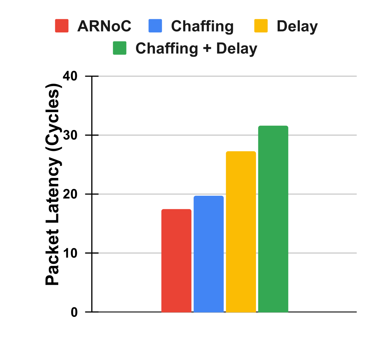
(a) Packet latency

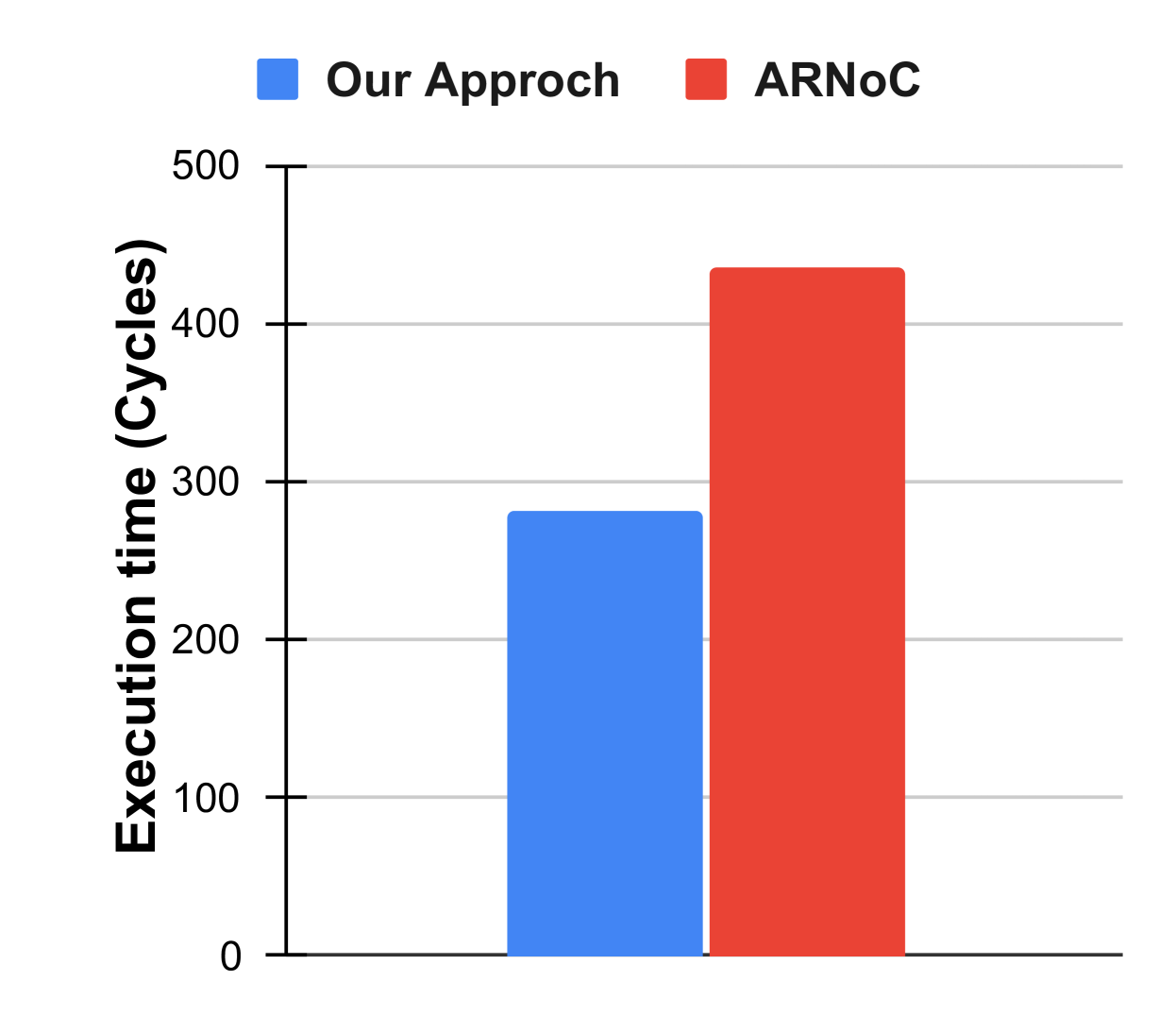
(b) Execution time

Figure 8. Comparison of proposed countermeasure versus ARNoC: (a) average packet latency of data transfer phase and (b) average execution time for tunnel creation phase.

In addition to low performance overhead, our lightweight anonymous routing has the inherent advantage of utilizing any adaptive routing mechanisms supported by NoC architectures (endpoint of output tunnel to the destination), while ARNoC cannot accommodate adaptive routing protocols because of having a pre-built tunnel from the source to destination.

Table 15. Comparison of the area and energy overhead between ARNoC and proposed countermeasure in NoC IP.

	ARNoC	Our Approach	Overhead
Area($\mu m^{2}$)	2914300	2957429	+ 1.47%
Energy($mJ$)	54.04	55.45	+ 2.6%

Table 15 compares the area and energy overhead of our lightweight countermeasure against ARNoC in 8$\times$8 mesh topology. In the implementation, our approach uses only the chaffing obfuscation. The energy consumption was calculated by averaging energy consumption of running FFT benchmark across all possible mappings of processing node and memory controller in mesh NoC-based SoC as discussed in Section 5.1.2. We observe 1.47% increase in area and 2.6% increase in energy. The area and energy overhead are negligible considering the performance improvement and additional security provided by our proposed anonymous routing compared to the state-of-the-art anonymous routing ARNoC (Charles et al., 2020).

6. Conclusion

Network-on-Chip (NoC) is a widely used solution for on-chip communication between Intellectual Property (IP) cores in System-on-Chip (SoC) architectures. Anonymity is a critical requirement for designing secure and trustworthy NoCs. In this paper, we made two important contributions. We proposed a machine learning-based attack that uses traffic correlation to break the state-of-the-art anonymous routing for NoC architectures. We developed a lightweight and robust anonymous routing protocol to defend against ML-based attacks. Extensive evaluation using real as well as synthetic traffic demonstrated that our ML-based attack can break anonymity with high accuracy (up to 99%) for diverse traffic patterns. The results also reveal that our lightweight countermeasure of obfuscating traffic with chaffing is robust against ML-based attacks with minor hardware overhead. The performance overhead of our proposed countermeasure is significantly less compared to the state-of-the-art anonymous routing for NoC-based SoCs.

References

- (1)
- Agarwal et al. (2009) N Agarwal et al. 2009. GARNET: A detailed on-chip network model inside a full-system simulator. ISPASS (2009).
- Ahmed et al. (2018) Alif Ahmed et al. 2018. Scalable hardware Trojan activation by interleaving concrete simulation and symbolic execution. In 2018 IEEE International Test Conference (ITC). IEEE, 1–10.
- Ahmed et al. (2021) M Meraj Ahmed, Abhijitt Dhavlle, Naseef Mansoor, Sai Manoj Pudukotai Dinakarrao, Kanad Basu, and Amlan Ganguly. 2021. What Can a Remote Access Hardware Trojan do to a Network-on-Chip?. In 2021 IEEE International Symposium on Circuits and Systems (ISCAS). IEEE, 1–5.
- Ahmed et al. (2020) M Meraj Ahmed, Abhijitt Dhavlle, Naseef Mansoor, Purab Sutradhar, Sai Manoj Pudukotai Dinakarrao, Kanad Basu, and Amlan Ganguly. 2020. Defense against on-chip trojans enabling traffic analysis attacks. In 2020 Asian Hardware Oriented Security and Trust Symposium (AsianHOST). IEEE, 1–6.
- Ampere (2022) Ampere. 2022. Ampere Altra Max 64-Bit Multi-Core Processor. https://amperecomputing.com/briefs/ampereone-family-product-brief. [Online].
- Bienia et al. (2008) Christian Bienia, Sanjeev Kumar, and Kai Li. 2008. Parsec vs. splash-2: A quantitative comparison of two multithreaded benchmark suites on chip-multiprocessors. In 2008 IEEE International Symposium on Workload Characterization. IEEE, 47–56.
- Binkert et al. (2011) N Binkert et al. 2011. The gem5 simulator. SIGARCH Computer Architecture News (2011).
- Boraten et al. (2016) Travis Boraten et al. 2016. Mitigation of denial of service attack with hardware Trojans in NoC architectures. In Parallel and Distributed Processing Symposium, 2016 IEEE International. IEEE, 1091–1100.
- Charles et al. (2020) S Charles et al. 2020. Lightweight Anonymous Routing in NoC based SoCs. In Design Automation & Test in Europe (DATE).
- Charles et al. (2021) S Charles et al. 2021. A Survey of Network-on-Chip Security Attacks and Countermeasures. ACM Computing Surveys (CSUR) 54, 5 (2021), 1–36.
- Charles and Mishra (2020) Subodha Charles and Prabhat Mishra. 2020. Lightweight and trust-aware routing in NoC-based SoCs. In 2020 IEEE Computer Society Annual Symposium on VLSI (ISVLSI). 160–167.
- Costan and Devadas (2016) Victor Costan and Srinivas Devadas. 2016. Intel SGX explained. Cryptology ePrint Archive (2016).
- Dhavlle et al. (2023) Abhijitt Dhavlle, M Meraj Ahmed, Naseef Mansoor, Kanad Basu, Amlan Ganguly, and Sai Manoj PD. 2023. Defense against On-Chip Trojans Enabling Traffic Analysis Attacks based on Machine Learning and Data Augmentation. IEEE Transactions on Computer-Aided Design of Integrated Circuits and Systems (2023).
- Dingledine et al. (2004) Roger Dingledine et al. 2004. Tor: The second-generation onion router. Technical Report. Naval Research Lab Washington DC.
- Farahmandi et al. (2019) Farimah Farahmandi et al. 2019. System-on-Chip Security: Validation and Verification. Springer Nature.
- Guo et al. (2019) Shengnan Guo, Youfang Lin, Shijie Li, Zhaoming Chen, and Huaiyu Wan. 2019. Deep spatial–temporal 3D convolutional neural networks for traffic data forecasting. IEEE Transactions on Intelligent Transportation Systems 20, 10 (2019), 3913–3926.
- Han and Moraga (1995) Jun Han and Claudio Moraga. 1995. The influence of the sigmoid function parameters on the speed of backpropagation learning. In From Natural to Artificial Neural Computation: International Workshop on Artificial Neural Networks Malaga-Torremolinos, Spain, June 7–9, 1995 Proceedings 3. Springer, 195–201.
- Intel (2023) Intel. 2023. 4th Gen Intel® Xeon® Scalable Processors. https://www.intel.com/content/www/us/en/products/docs/processors/xeon-accelerated/4th-gen-xeon-scalable-processors-product-brief.html. [Online].
- JS et al. (2015) Rajesh JS et al. 2015. Runtime detection of a bandwidth denial attack from a rogue network-on-chip. In Proceedings of the 9th International Symposium on Networks-on-Chip. ACM, 8.
- Lyu et al. (2020) Yangdi Lyu et al. 2020. Scalable Activation of Rare Triggers in Hardware Trojans by Repeated Maximal Clique Sampling. IEEE Transactions on Computer-Aided Design of Integrated Circuits and Systems (2020).
- Mishra et al. (2021) Prabhat Mishra et al. 2021. Network-on-Chip Security and Privacy. Springer Nature.
- Mishra et al. (2017) Prabhat Mishra, Swarup Bhunia, and Mark Tehranipoor. 2017. Hardware IP security and trust. Springer.
- Nasr et al. (2018) M Nasr et al. 2018. Deepcorr: Strong flow correlation attacks on Tor using deep learning. In Proceedings of the 2018 ACM SIGSAC Conference on Computer and Communications Security. 1962–1976.
- Sakalis et al. (2016) Christos Sakalis, Carl Leonardsson, Stefanos Kaxiras, and Alberto Ros. 2016. Splash-3: A properly synchronized benchmark suite for contemporary research. In 2016 IEEE International Symposium on Performance Analysis of Systems and Software (ISPASS). IEEE, 101–111.
- Sarihi et al. (2021) A Sarihi et al. 2021. Securing network-on-chips via novel anonymous routing. In Proceedings of the 15th IEEE/ACM International Symposium on Networks-on-Chip.
- Schmidhuber (2015) Jürgen Schmidhuber. 2015. Deep learning in neural networks: An overview. Neural networks 61 (2015), 85–117.
- Sinha et al. (2021) M Sinha et al. 2021. Sniffer: A Machine Learning Approach for DoS Attack Localization in NoC-based SoCs. IEEE Journal on Emerging and Selected Topics in Circuits and Systems (2021).
- Sudusinghe et al. (2021) C Sudusinghe et al. 2021. Denial-of-service attack detection using machine learning in network-on-chip architectures. In Proceedings of the 15th IEEE/ACM International Symposium on Networks-on-Chip. 35–40.
- Wang et al. (2020) K Wang et al. 2020. Tsa-noc: Learning-based threat detection and mitigation for secure network-on-chip architecture. IEEE Micro 40, 5 (2020), 56–63.
- Weerasena and Mishra (2023) Hansika Weerasena and Prabhat Mishra. 2023. Security of Electrical, Optical and Wireless On-Chip Interconnects: A Survey. ACM Trans. Des. Autom. Electron. Syst. (oct 2023). https://doi.org/10.1145/3631117
- Woo et al. (1995) Steven Cameron Woo, Moriyoshi Ohara, Evan Torrie, Jaswinder Pal Singh, and Anoop Gupta. 1995. The SPLASH-2 programs: Characterization and methodological considerations. ACM SIGARCH computer architecture news 23, 2 (1995), 24–36.
- Yu et al. (2013) Q Yu et al. 2013. Exploiting error control approaches for hardware trojans on network-on-chip links. In International symposium on defect and fault tolerance in VLSI and nanotechnology systems (DFTS). 266–271.
- Zantout et al. (2011) Bassam Zantout, Ramzi Haraty, et al. 2011. I2P data communication system. In Proceedings of ICN. Citeseer, 401–409.
- Zhao et al. (2017) B Zhao et al. 2017. Convolutional neural networks for time series classification. Journal of Systems Engineering and Electronics 28, 1 (2017), 162–169.