Improving Autonomous Driving Safety with POP: A Framework for Accurate Partially Observed Trajectory Predictions

Abstract

Accurate trajectory prediction is crucial for safe and efficient autonomous driving, but handling partial observations presents significant challenges. To address this, we propose a novel trajectory prediction framework called Partial Observations Prediction (POP) for congested urban road scenarios. The framework consists of two stages: self-supervised learning (SSL) and feature distillation. In SSL, a reconstruction branch reconstructs the hidden history of partial observations using a mask procedure and reconstruction head. The feature distillation stage transfers knowledge from a fully observed teacher model to a partially observed student model, improving prediction accuracy. POP achieves comparable results to top-performing methods in open-loop experiments and outperforms the baseline method in closed-loop simulations, including safety metrics. Qualitative results illustrate the superiority of POP in providing reasonable and safe trajectory predictions. Demo videos and code are available at https://chantsss.github.io/POP/.

I Introduction

The rapid development of autonomous vehicles has brought a myriad of challenges and opportunities to both academia and industry in recent years. One of the critical aspects of self-driving technology is vehicle trajectory prediction, which provides valuable information for autonomous vehicles to assess potential risks and make informed decisions in dynamic traffic situations. Challenges in this domain include the dynamic and unpredictable nature of traffic, interactions between road users, diverse driving behaviors, sensor occlusions, and limitations. Recently, data-driven approaches exhibited promising performance in prediction accuracy on challenges [1][2]. A motion forecasting model typically collects comprehensive information from perception signals and highdefinition (HD) maps, such as traffic light states, motion history of agents, and the road graph. The most state-of-the-art prediction models adopt Transformers [3][4][5] or graph neural networks (GNNs) [6][7] to encode agent-agent and agent-map interactions have achieved outstanding prediction accuracy. Some researchers proposed to employ Self-supervised learning (SSL) to train a network for more transferable, generalizable, and robust representation learning. For example, SSL-Lanes[8] and PreTraM[9] demonstrated that carefully designed pretext tasks can significantly enhance performance without using extra data by learning richer features.

However, these methods focus solely on fitting an inference model on a dataset with a neural network, without considering the mismatch between the distribution of the actual noisy data from the upstream module and the clean data provided on the dataset. This mismatch is due to the limitations of the sensing and tracking system equipment and algorithms in the real world, which is known as the sim-2-real problem. Some works have explored how to improve the robustness of predictors from the perspective of input noise[10][11], but they have neglected a key phenomenon in practical applications, namely, domain shift due to insufficient observation data, which is common to see in autonomous driving scenarios.

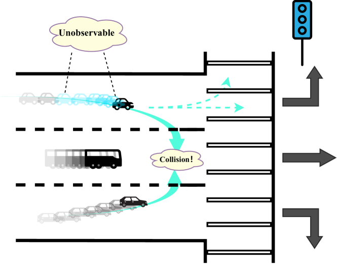
Figure 1: Partially observable in practical application scenarios. In this scenario, the self-driving car was making a right turn, but another car unexpectedly turned right from the left turn lane. Due to insufficient observation, the prediction algorithm provided inaccurate future trajectories for it, leading to a dangerous situation as the self-driving car’s planning ignored the other car.

In concrete terms, most current learning-based prediction algorithms require a fixed-length history trajectory as output, as per the popular challenge setting. For example, Argoverse 1 (Av1)[1] provides 2 seconds of history information, while Argoverse 2 (Av2)[2] requires 5 seconds of observations as input for longer-term prediction tasks. However, such algorithms developed under this fixed input length setting cannot handle real-world applications where only partial observations are available. For instance, if a previously obscured vehicle suddenly appears in the view of the ego vehicle, the predictor’s inability to accurately predict its future trajectory due to insufficient observation length can lead to a collision risk, as shown in Fig.1. In a later section, we analyze upstream tracking and perception data to expose this key issue. We argue that even the most advanced architectures specialized for this task fail to process variable observation lengths. Alessio et al.[12] propose a distillation framework that recovers a reliable proxy of the same information obtained with more input observations, but it still only supports a fixed observation length. To address this problem, we propose a new hierarchical prediction framework that can handle dynamic observation lengths by introducing an SSL mask strategy to a history reconstruction pretext task. Additionally, we employ a feature distillation scheme to transfer future extraction ability to the student model. Our contributions are summarized as follows:

• Our study uncovers the critical challenge of performance degradation when utilizing prediction algorithms in the case of insufficient observations, which even the most robust baseline cannot address. To our knowledge, this is the first comprehensive analysis of the partial observations problem for state-of-the-art (SOTA) prediction methods in autonomous driving scenarios.

• We propose a flexible prediction algorithm, the POP (Partial Observations Prediction) framework, which can handle partial observations as long as they exceed one frame while maintaining high prediction accuracy. The framework comprises two key stages: SSL and feature distillation, enabling the model to effectively utilize partial observations for accurate trajectory prediction.

• The proposed method is thoroughly evaluated on real-world datasets and a closed-loop simulator. Evaluation results demonstrate that the POP framework achieves comparable or superior performance in terms of prediction accuracy and safety metrics compared to existing state-of-the-art methods.

II Related Work

II-A Feature distillation in Motion Forecasting

The idea of knowledge distillation is first brought up by Hinton etal. [13] to transfer knowledge from a large, complex model (teacher) to a smaller, simpler model (student) for model compression purpose. In the context of trajectory forecasting, knowledge distillation has been used to make a model immune to incorrect detection, tracking, fragmentation, and corruption of trajectory data in crowded scenes, by distilling knowledge from a teacher with longer observation to a student with much fewer observations[12]. Although the performance is nearly retained though. This is not reasonable in more challenging autonomous driving scenes when we have longer observations(e.g. 49 frames) and only pick the first 2 frames and throw the others useful information. Inspired by [14], our aim is not to compress a model yet to improve its performance. This procedure is usually referred to as self-distillation, since the student network shares the same architecture of its teacher. Similarly to [15], our approach sets up asymmetric networks: the student is encouraged to overcome its knowledge gap by following the guide of its teacher, eventually boosting its performance. This is done in the specific context of trajectory forecasting, and we demonstrate that knowledge distillation can lead to effective predictions even when the model has access to very few observations.

II-B SSL:Self-supervised Learning in Motion Forecasting

Self-supervised learning (SSL) has been widely explored and utilized in various research domains[16, 17]. SSL leverages the inherent structure or patterns present in unlabeled data to learn useful representations or tasks. In previous trajectory prediction work, SSL has shown promising capabilities in improving the prediction accuracy. PreM[9] focuses on connecting trajectory and scene context, enhancing their representations for trajectory forecasting. They do not have the task of reconstructing history. A recent work FMAE[18] proposes to mask agents’ trajectories and lane segments and reconstruct masked elements using a prediction head, at last fine tune the motion forecasting task. However, his reconstruction mechanism is in terms of the whole trajectory. In contrast, in our proposed method, we use to take the state under each time step as the unit of reconstruction, which is more in line with the POP situation in reality. A very recent work[19] used a temporal decay module to imputate the missing observation, and treat the imputation as a training objective that is jointly optimized with the motion forecasting task. What’s more, it neglects the effectiveness of reconstructing missing observations to planning task. This is extremely vital for safe autonomous driving systems, and we will elaborate on this later in the experimental module.

III Problem Formulation

We adopt a structured vectorized representation to depict the map and agents. We denote the past trajectories of agents as $X_{H}=\{x_{i}\}$, where $x_{i}\in\mathbb{R}^{T_{H}\times D}$ indicating the location, yaw angle, and velocity of agent $i$ at previous $T_{H}$ time steps. The road map is denoted as $L=\{l_{i}\}$, where $l_{i}\in\mathbb{R}^{N\times F}$ representing $i_{th}$ lane has $N$ segment and each segment has $F$ lane semantic attributes (e.g., intersections and crosswalks). The forecasting task aims to generate $T_{F}$ steps future trajectories :

$$Y_{F}=f(X_{H}*M_{H},L),$$ (1)

where $M_{H}=\{m_{i}\}$, where $m_{i}\in\mathbb{R}^{T_{H}\times 1}$ indicating the validity for history state at previous $T_{H}$ time steps. In contrast to the previous definition of trajectory prediction, we consider that the history trajectory of the focal agent does not necessarily satisfy completeness, and thus we set ${m^{T_{H}}_{i}}=0$ for states that are not valid at $T_{H}$.

IV Methodology

IV-A Overview

The overview of our framework is shown above Fig.2. Our prediction framework comprises three stages. In the first stage, we train a teacher model using complete observations. The inference stage is the standard prediction process: ha and hm features are generated using roadmaps and history states through an encoder consisting of a multi-layer perceptron (MLP) and a location embedding layer; a series of attention modules are used to capture the interaction information between elements, and the decoder generates an initial guess for the future trajectory. During the SSL stage, we enable a mask procedure and use partial observations as input, along with a history reconstruction pre-task to reconstruct missing observations. In the Distillation step, we freeze the teacher model’s parameters and the feature distillation strategy is used to transfer knowledge to intermediate features of partial observations, while keeping the mask procedure on. It is worth noting that, unlike previous SSL approaches that aim to improve predictor performance with complete observations, we consider the distillation task with partial observations as the final fine-tuning task.

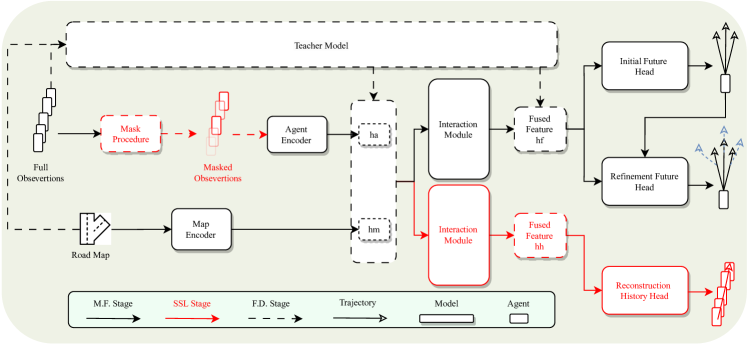
Figure 2: Overview scheme of POP. Our method consists of three stages. The motion forecasting stage involves training a teacher model with complete observations. The SSL stage consists a mask procedure and a history reconstruction pre-task. During the Distillation stage, the teacher model’s parameters are frozen, and the feature distillation strategy is used to transfer knowledge to intermediate features of partial observations.

IV-B Motion Forecasting Stage

In this stage We follow the inference pipeline of QCNet[4] and consider it as a strong baseline in experiments in the later section. We build a local spacetime coordinate system for each scene element to encode scene representations. These representations are transformed to Fourier features and passed through an MLP to obtain relative positional embeddings $R$. Factorized attention and self-attention mechanisms are applied to $\{X_{H},R\}$ and $\{L,R\}$ respectively to obtain hidden encoded features $ha$ and $hm$. We adopt the architecture of detection transformer in both the initial and refinement decoder modules to address the one-to-many problem, allowing multiple learnable queries to cross-attend the scene encodings and a MLP to decode trajectories. A slight difference in refinement decoder is that a gated recurrent unit is used to embed each trajectory anchor, and we take its final hidden state as the mode query. Taking the output of the proposal module as anchors, we let the refinement module predict the offset to the proposed trajectories and estimate the likelihood of each hypothesis.

IV-C Self-supervised learning Stage

Recall the motivation, our aim is to make predictors robust to insufficient observations. An intuitive to achieve this goal is to add noise or perform data augmentation. Since the partial observation phenomenon varies from time to time, we are not accessible to a uniform real-world noise distribution. Thus we build a pretext task from reconstructing the random masked input history. Specifically, a mask procedure and a reconstruction branch is built when performing the SSL stage. It is similar to the future prediction branch structurally. it only differs from the output dimension of decoder head, which means we use $T_{H}$ as the prediction horizon.

IV-D Feature Distillation Stage

In order to maintain the predictive capabilities of teachers in the face of insufficient observations, our training strategy involves transferring knowledge from the entire input sequence. To achieve this, we manipulate hidden features from both the encoder and decoder. Specifically, we ensure that all of the student’s features correspond to those in the teacher network. This is accomplished through a feature distillation loss, which is defined as the mean squared error (MSE) between the two feature representations:

$$\mathcal{L_{D}}=\frac{1}{d}\sum\left\|(h^{T}-h^{S})\right\|^{2},$$ (2)

where $d$ is the dimension of the corresponding feature representations, $h^{S}=\{h_{a}^{S},h_{m}^{S},h_{f}^{S}\}$, $h^{T}=\{h_{a}^{T},h_{m}^{T},h_{f}^{T}\}$. The feature distillation loss encourages the student model to learn feature representations that are similar to those of the teacher model.

IV-E Training Objectives

Our goal is to build, in three steps, a model capable of accurately predicting future locations when only partial observations are available. To train the teacher model in the first stage, we employ negative log-likelihood loss and winner-take-all training strategy to optimize the best-predicted future trajectory. The training loss in this stage is:

$$\mathcal{L_{MF}}=\mathcal{L}_{init}+\mathcal{L}_{refine}+\alpha\mathcal{L}_{cls},$$ (3)

where the classification loss is added to optimize the mixing coefficients and $\alpha$ is parameter to balance regression and classification.

$$\mathcal{L_{SSL}}=\mathcal{L_{MF}}+\beta\mathcal{L}_{recons},$$ (4)

$$\mathcal{L_{FD}}=\mathcal{L_{MF}}+\lambda\mathcal{L}_{D}.$$ (5)

When perform SSL stage or feature distillation stage, we keep the $L_{MF}$ and add a reconstruction loss or distillation loss with balance parameter $\beta$ or $\lambda$ respectively as shown in Eq.4 and Eq.5.

V Preliminary Analysis

Before diving into the experiment section, we will explore two questions to recall the motivation and further validate the effectiveness of the proposed method. First of all, is it common to see inefficient observation situations in the real world? Secondly, are existing SOTA trajectory prediction methods able to handle the partial observation problem?

V-A Observation Distribution Analysis

To answer the first question, we investigate the Av1 tracking dataset, which is a collection of 113 log segments with 3D object tracking annotations. These log segments vary in length from 15 to 30 seconds and collectively contain a total of 11,052 tracks. We use an open-source tracking baseline method [20], which achieved 1st place on the Argoverse 3D tracking test set. According to the Av1 motion forecasting challenge standard, 20 frames are used for a complete observation. We construct each segment of the observation frame by frame from the beginning of the appearance of the target until the target disappears. Fig. 3 shows the distribution of the observation, indicating that the prediction algorithm for autonomous driving applications is often unable to satisfy the complete 20-frame observations on the dataset due to occlusion, limitations in sensing range, and large speed differences between vehicles.

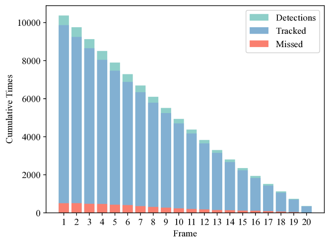
Figure 3: Distribution of observations with standard 20 frames. The gray bars represent the detection of each frame for a fixed observation period, while the blue bars represent tracking. Red indicates tracking failure resulting from occlusion, insufficient sensing range, etc.

V-B Observation Length Evaluation Analysis

We evaluated the MinADE₅ performance of three popular prediction algorithms when provided with observations of varying lengths on the validation set of Av1 and Av2. As depicted in Fig.4, it is evident that the predictor’s performance is directly correlated with the length of the observations. In other words, the more information from observations used as input, the greater the accuracy of the predictions made by the predictor. This relationship is especially pronounced when dealing with long prediction horizon task. Therefore, we conclude that the currently available state-of-the-art trajectory prediction methods are unable to effectively handle situations with partial observations.

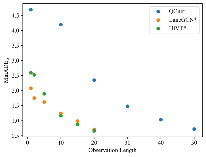
Figure 4: Observation length evaluation analysis on Av1 and Av2. Methods that are evaluated on Av1 are marked with symbol “*”

VI Experimental Results

VI-A Open Loop Experiment

VI-A1 Dataset

We evaluate our method on both Av1 and Av2. The former requires a 2s history input and a 3s future trajectory output, and the latter one focuses on a long term 6s prediction and a longer corresponding 5s history input.

VI-A2 Metrics

For open loop evaluation, we use the official benchmark metrics, including minADE_k, minFDE_k, MR_k, and brier-minFDE_k. These metrics are calculated based on the trajectory with the closest endpoint to the ground truth over $k$ trajectory predictions.

VI-A3 Implementation Details

We train the model for all experiments using cosine learning rate decay with a weight decay of 0.0001 on 4 RTX3090 and set the initial learning rate to 0.0005. We use the pre-trained model provided in the officially released checkpoint. $\alpha$, $\beta$, $\lambda$ are set to 1, 0.5, 0.5 respectively. Due to the variations in road structures and traffic rules across different regions, a generalized observation distribution cannot be obtained. To address this, we have employed a random drop scheme during training. No data augmentation or model ensemble techniques are applied.

VI-A4 Comparison with State-of-the-Art

We compared our method to the state-of-the-art without ensembles on the Av2 test set in the single-agent setting, and the results are reported in Table III (upper group). Our method achieves results comparable to the best-performing methods, ranking third on the minADE₆ metric without using the ensemble technique. Our performance is also comparable to that of F-MAE[18], which uses the SSL strategy under complete observation conditions. In later experiments, we will demonstrate the superiority of POP under partial observation conditions. To evaluate the generalization of our method, we conducted experiments on the Av1 test set using HiVT as the backbone. Although our POP-H performance is slightly degraded compared to HiVT[5], this is due to the use of incomplete observations to train the predictor, which increases the difficulty of fitting the network. Nonetheless, our performance is still comparable to the SOTA methods, such as LED[21] and mmTrans[22].

TABLE I: Closed-loop Simulation Results on Interaction

Method	P-K	DIST$\uparrow$	JERK$\downarrow$	RC$\downarrow$	CT$\downarrow$	RCT$\downarrow$
HiVT	1	30.19	3.23	0.657	7	1
HiVT	3	28.80	2.87	0.636	2	1
POP-H	1	30.97	4.07	0.641	5	0
POP-H	3	28.38	3.07	0.616	1	1
HiVT	1	40.77	3.24	0.608	21	5
POP-H	1	41.35	3.50	0.576	17	4

• The top group records performance in 91 scenarios, while the bottom group represents the performance in all.
  

TABLE II: Open-loop Simulation Results on Interaction

Model	minADE1	minFDE1	RminADE1	RminFDE1
HiVT	2.51	5.21	3.22	8.18
POP-H	2.54	6.23	2.66	6.30

• Note that the two metrics RminADE₁, RminFDE₁ were collected with randomly reduced observation lengths.
  

TABLE III: Comparison with State-of-the-Art Methods on the Argoverse test set.

Model	minADE6	minADE1	minFDE6	minFDE1	brier-minFDE6	MR1	MR6
GANet[23]	0.72	1.77	1.34	4.48	1.96	0.17	0.59
MTR[24]	0.73	1.74	1.44	4.39	1.98	0.15	0.58
GoRela[25]	0.76	1.82	1.48	4.62	2.01	0.22	0.66
F-MAE[18]	0.71	1.74	1.39	4.36	2.03	0.17	0.61
QCNet[4]	0.65	1.69	1.29	4.30	1.91	0.16	0.59
POP-Q (ours)	0.72	1.86	1.46	4.84	2.08	0.20	0.61
LaneGCN[7]	0.87	1.71	1.36	3.78	2.05	0.59	0.16
mmTrans[22]	0.84	1.77	1.34	4.00	2.03	0.61	0.15
LTP[21]	0.83	1.62	1.30	3.55	1.86	0.56	0.15
HiVT[5]	0.77	1.60	1.17	3.53	1.84	0.55	0.13
ADAPT[26]	0.79	1.59	1.17	3.50	1.80	0.54	0.12
POP-H (ours)	0.83	1.73	1.32	3.83	1.99	0.59	0.15

TABLE IV: Ablation study of minADE/minFDE among different training strategies on the Argoverse validation set.

	Training strategy		minADE6/minFDE6
Scratch	SSL	Distill.	Obs=1	Obs=10	Obs=20	Obs=30	Obs=40	Obs=50	Obs=random
✓			4.69/8.79	4.28/7.52	2.48/4.78	1.54/3.13	1.05/2.08	0.72/1.25	2.37/4.43
✓	✓		4.03/7.45	2.31/4.27	1.10/2.05	0.93/1.72	0.85/1.57	0.79/1.45	1.47/2.72
✓		✓	4.04/7.48	2.37/4.37	1.19/2.25	1.00 /1.88	0.93/1.75	0.88/1.66	1.52/2.83
✓	✓	✓	4.03/7.44	2.24/4.16	1.12/2.08	0.92/1.70	0.84/1.54	0.79/1.45	1.42/2.61

VI-A5 Ablation Study

We conducted ablation studies on the Av2 validation set using the QCNet pretrained checkpoint. Our results show that the QCNet model performs poorly with partial observations. In particular, when fewer than 30 frames are available, the prediction error increases to two times compared to when the full observations are input. However, when using either the SLL or Distill strategies individually, the performance of the predictor shows a notable improvement in the POP case. This highlights the effectiveness of both stages in our design. While the SLL-only strategy achieves the same level of performance as the POP strategy with complete observations, POP outperforms SLL when there are less than 50 observations. Our findings suggest that feature distillation, treated as a fine-tuning task after SLL, allows for continuous feature learning and better performance.

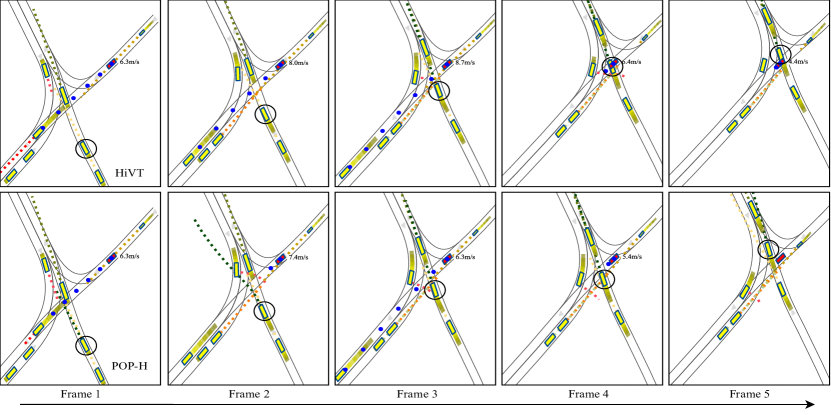
Figure 5: A collision scenario caused by limited observations. The AV (red) is surrounded by yellow vehicles, with its planned trajectory (blue scatter line) and predicted trajectories of other vehicles (various-colored scatter lines) displayed. Due to limited observations, the HiVT predictor inaccurately predicted the future trajectory of a vehicle (black circle), causing the AV to accelerate and ultimately collide. In contrast, the AV equipped with the POP-H predictor exhibited superior predictions, ensuring safety.

VI-B Closed Loop Experiment

VI-B1 Simulation Setting

In our closed-loop simulation, we limit our predictions to neighboring vehicles within a 50m radius of the AV, considering the limited field-of-view and perception range of autonomous vehicles in real-world scenarios. At each step, we use POP-H or HiVT to predict the future trajectories of agents over a 6.0-second horizon with a 0.5-second interval. The planning process for collision check directly incorporates the K most probable prediction outcomes for each agent. The prediction model is pre-trained using feature data extracted from the closed-loop simulation itself, consisting of approximately 15,072 files. Each simulated scenario incorporates a designated task route to evaluate the planning performance, as shown in Fig. 5. The collision avoidance planner guides the AV along the provided task route. If the implemented algorithm fails to identify a valid solution, the AV executes a stop behavior along the generated path with a deceleration of $-4.0\,m/s^{2}$. All other agents are controlled by the intelligent driver model.

VI-B2 Metrics

We compare algorithms using the following metrics: DIST: Average completion distance of AV along the given route in each scenario. JERK: Average jerk cost reflecting the planned trajectory’s smoothness. RC: Reaction cost of other traffic agents, defined as the average deceleration efforts of nearby agents within a 40-meter range. CT: Total number of valid collision times experienced by AV, excluding collisions at the rear and collisions with agents when AV is stationary. RCT: Collision times at the rear of AV.

VI-B3 Quantitive Results

We present the open-loop prediction performance of HiVT and POP-H in Table II, focusing on MinADE₁ and MinFDE₁ since we use the most likely prediction trajectory for collision checking in the closed-loop simulation. Results show that vanilla HiVT’s performance significantly drops with random observations, while POP-H remains stable under both complete and incomplete observations due to our design for handling incomplete observations during training. The closed-loop Results are reported in Table I. For each metric, the best result is in bold, and the worst result is underlined. In the closed-loop simulation, our proposed method outperforms HiVT in almost all metrics, particularly in safety, with a 25% reduction in collisions. HiVT yielded slightly better jerk results but at the cost of less driving distance and a higher number of collisions. We achieved favorable performance in 91 high interactivity scenarios, particularly when using 3 predicted trajectories for collision detection. POP-H reduced collisions to 1 and achieved the lowest RC, facilitating friendly driving to other vehicles. The closed-loop Results are reported in Table I. For each metric, the best result is in bold and the worst result is underlined.

VI-B4 Qualitative Results

We demonstrate a scenario in our simulator where a self-driving vehicle navigates through a congested traffic intersection, as shown in Figure LABEL:fig. During the initial phase of the simulation, the AV intends to traverse the intersection with a planned speed of 6.3 m/s. However, due to insufficient observation, the HiVT predictor inaccurately predicts the future trajectory in the first two frames. As a result, the AV fails to account for the movement of the vehicle below and begins to accelerate. By frame 3, the speed has already reached 8.7 m/s, making it too late to decelerate and leading to a collision. In contrast, the AV with the POP-H predictor consistently provides more reasonable predictions (indicated by the black scatter line) from frame 1 to frame 5, ensuring a higher level of safety.

VII CONCLUSIONS

In this work, we addressed the main issue of sim-to-real in trajectory prediction for autonomous driving. We argued that even state-of-the-art predictors failed to consider incomplete observations when designing predictions for real-world applications. To bridge this gap, we proposed a novel prediction framework that employed SSL to help the final model learn to build hidden history representations. We also utilized feature distillation to transfer knowledge from a teacher model pre-trained with complete observations to a student model with few observations. Various experiments on open-loop datasets and closed-loop simulations verified the effectiveness of each component of our method.

References

- [1] M.-F. Chang, J. W. Lambert, P. Sangkloy, J. Singh, S. Bak, A. Hartnett, D. Wang, P. Carr, S. Lucey, D. Ramanan, and J. Hays, “Argoverse: 3d tracking and forecasting with rich maps,” in Conference on Computer Vision and Pattern Recognition (CVPR), 2019.
- [2] B. Wilson, W. Qi, T. Agarwal, J. Lambert, J. Singh, S. Khandelwal, B. Pan, R. Kumar, A. Hartnett, J. K. Pontes, D. Ramanan, P. Carr, and J. Hays, “Argoverse 2: Next generation datasets for self-driving perception and forecasting,” in Proceedings of the Neural Information Processing Systems Track on Datasets and Benchmarks (NeurIPS Datasets and Benchmarks 2021), 2021.
- [3] Z. Huang, H. Liu, and C. Lv, “Gameformer: Game-theoretic modeling and learning of transformer-based interactive prediction and planning for autonomous driving,” 2023.
- [4] Z. Zhou, J. Wang, Y.-H. Li, and Y.-K. Huang, “Query-centric trajectory prediction,” in Proceedings of the IEEE/CVF Conference on Computer Vision and Pattern Recognition (CVPR), 2023.
- [5] Z. Zhou, L. Ye, J. Wang, K. Wu, and K. Lu, “Hivt: Hierarchical vector transformer for multi-agent motion prediction,” in Proceedings of the IEEE/CVF Conference on Computer Vision and Pattern Recognition (CVPR), 2022.
- [6] X. Wang, T. Su, F. Da, and X. Yang, “Prophnet: Efficient agent-centric motion forecasting with anchor-informed proposals,” 2023.
- [7] M. Liang, B. Yang, R. Hu, Y. Chen, R. Liao, S. Feng, and R. Urtasun, “Learning lane graph representations for motion forecasting,” in ECCV, 2020.
- [8] P. Bhattacharyya, C. Huang, and K. Czarnecki, “Ssl-lanes: Self-supervised learning for motion forecasting in autonomous driving,” 2022.
- [9] C. Xu, T. Li, C. Tang, L. Sun, K. Keutzer, M. Tomizuka, A. Fathi, and W. Zhan, “Pretram: Self-supervised pre-training via connecting trajectory and map,” 2022.
- [10] Q. Zhang, S. Hu, J. Sun, Q. A. Chen, and Z. M. Mao, “On adversarial robustness of trajectory prediction for autonomous vehicles,” 2022.
- [11] Y. Cao, D. Xu, X. Weng, Z. Mao, A. Anandkumar, C. Xiao, and M. Pavone, “Robust trajectory prediction against adversarial attacks,” 2022.
- [12] A. Monti, A. Porrello, S. Calderara, P. Coscia, L. Ballan, and R. Cucchiara, “How many observations are enough? knowledge distillation for trajectory forecasting,” 2022.
- [13] G. Hinton, O. Vinyals, and J. Dean, “Distilling the knowledge in a neural network,” 2015.
- [14] L. Zhang, J. Song, A. Gao, J. Chen, C. Bao, and K. Ma, “Be your own teacher: Improve the performance of convolutional neural networks via self distillation,” 2019.
- [15] A. Porrello, L. Bergamini, and S. Calderara, “Robust re-identification by multiple views knowledge distillation,” 2020.
- [16] Y. You, T. Chen, Z. Wang, and Y. Shen, “When does self-supervision help graph convolutional networks?” 2020.
- [17] Y. Liu, M. Jin, S. Pan, C. Zhou, Y. Zheng, F. Xia, and P. Yu, “Graph self-supervised learning: A survey,” IEEE Transactions on Knowledge and Data Engineering, pp. 1–1, 2022. [Online]. Available: https://doi.org/10.1109%2Ftkde.2022.3172903
- [18] J. Cheng, X. Mei, and M. Liu, “Forecast-MAE: Self-supervised pre-training for motion forecasting with masked autoencoders,” Proceedings of the IEEE/CVF International Conference on Computer Vision, 2023.
- [19] Y. Xu, A. Bazarjani, H. gun Chi, C. Choi, and Y. Fu, “Uncovering the missing pattern: Unified framework towards trajectory imputation and prediction,” 2023.
- [20] J. Lambert, “Open argoverse cbgs-kf tracker,” https://github.com/johnwlambert/argoverse˙cbgs˙kf˙tracker, 2020.
- [21] J. Wang, T. Ye, Z. Gu, and J. Chen, “Ltp: Lane-based trajectory prediction for autonomous driving,” in Proceedings of the IEEE/CVF Conference on Computer Vision and Pattern Recognition, 2022, pp. 17 134–17 142.
- [22] Y. Liu, J. Zhang, L. Fang, Q. Jiang, and B. Zhou, “Multimodal motion prediction with stacked transformers,” 2021.
- [23] M. Wang, X. Zhu, C. Yu, W. Li, Y. Ma, R. Jin, X. Ren, D. Ren, M. Wang, and W. Yang, “Ganet: Goal area network for motion forecasting,” 2023.
- [24] S. Shi, L. Jiang, D. Dai, and B. Schiele, “Motion transformer with global intention localization and local movement refinement,” 2023.
- [25] A. Cui, S. Casas, K. Wong, S. Suo, and R. Urtasun, “Gorela: Go relative for viewpoint-invariant motion forecasting,” 2022.
- [26] G. Aydemir, A. K. Akan, and F. Güney, “ADAPT: Efficient multi-agent trajectory prediction with adaptation,” in Proceedings of the IEEE/CVF International Conference on Computer Vision, 2023.