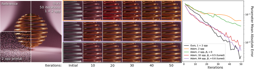
Figure 1. We simultaneously optimise the spiral’s base colour, metalness and roughness. Our gradient meta-estimator quickly recovers the gradient with just one finite-difference and two proportional samples per pixel. Adam’s default first moment estimator ($\beta_{1}=0.9$) cannot adapt as quickly and often overshoots. After tuning Adam’s hyperparameters for this specific problem, it approaches out method at 32 spp and matches it only at 64 spp. Banner 2 © 2023 Wenzel Jakob

Joint Sampling and Optimisation for Inverse Rendering

Abstract.

When dealing with difficult inverse problems such as inverse rendering, using Monte Carlo estimated gradients to optimise parameters can slow down convergence due to variance. Averaging many gradient samples in each iteration reduces this variance trivially. However, for problems that require thousands of optimisation iterations, the computational cost of this approach rises quickly.

We derive a theoretical framework for interleaving sampling and optimisation. We update and reuse past samples with low-variance finite-difference estimators that describe the change in the estimated gradients between each iteration. By combining proportional and finite-difference samples, we continuously reduce the variance of our novel gradient meta-estimators throughout the optimisation process. We investigate how our estimator interlinks with Adam and derive a stable combination.

We implement our method for inverse path tracing and demonstrate how our estimator speeds up convergence on difficult optimisation tasks.

1. Introduction

Forward rendering involves solving the light transport integrals with given scene parameters, e.g., geometry, materials, textures, by numerically estimating the rendering equation (Kajiya, 1986; Pharr et al., 2016). Inverse rendering reverses this process by estimating the scene parameters starting from a given target image. This process involves inverting the rendering equation (Kajiya, 1986).

Such inversion tasks are typically solved by gradient descent. Physically-based differentiable renderers (Jakob et al., 2022; Li et al., 2018; Zhang et al., 2020) facilitate these gradient-based optimisation methods. The process involves backpropagating from an underlying loss function, quantifying the disparity between an image generated with the current parameters and the target image, resulting in gradients w.r.t. the scene parameters. These gradient values are approximated from a given set of samples, and subsequently, the scene parameters are adjusted using these gradients to minimise the loss. The ultimate goal is to converge to a parameter set that produces the target image. Due to the nature of Monte Carlo integration, the estimated gradients can be extremely noisy, hampering the performance of gradient-based optimisers. In inverse rendering, gradients are estimated with tens to hundreds of rays traced per pixel (Nimier-David et al., 2020; Zhang et al., 2019) to minimise noise. Usually, inverse rendering requires hundreds to thousands of iterations to converge; recomputing these gradient estimates in every iteration comes at a large cost.

In this paper, we propose a theoretical framework that jointly considers sampling and optimisation by deriving a theoretical framework for interleaving them. We reuse past samples without introducing bias thanks to finite-difference estimators that describe the change in the estimated gradients between each iteration. By combining proportional and finite-difference samples, we continuously reduce the variance of our novel gradient meta-estimators throughout the optimisation process.

First, we introduce our meta-estimation theory and then discuss our variance estimation strategies used to derive coefficients for our meta-estimator. We investigate how our estimator interlinks with Adam and derive a stable combination. We run experiments to evaluate our method in the context of inverse rendering. Finally, we discuss our method concerning future and concurrent work and give our conclusions.

Our contributions include:

• Meta-estimation theory on combining proportional and finite-difference estimators.

• Practical variance approximation techniques to effectively implement meta-estimation.

• Implementation and evaluation of meta-estimation for inverse rendering. (We will release our code upon acceptance.)

2. Related work

Differentiable Path Tracing

Path tracing accounts for global illumination through physically accurate light transport by Monte Carlo integration of the rendering equation (Kajiya, 1986). Recent works proposed various approaches to differentiate such Monte Carlo integrals and estimate derivatives w.r.t. scene parameters. (Nimier-David et al., 2020; Zeltner et al., 2021; Jakob et al., 2022; Li et al., 2018; Zhang et al., 2020). While our work applies to any method using gradient descent on Monte Carlo estimated gradients, we mainly experiment with Path Replay Backpropagation (Vicini et al., 2021); a well-established state-of-the-art method for inverse path tracing, implemented in Mitsuba 3 (Jakob et al., 2022).

Previous works have focused on sampling strategies (Zhang et al., 2021; Yan et al., 2022; Bangaru et al., 2020) and improving the optimisation itself (Nimier-David et al., 2020; Vicini et al., 2021) to reduce noise in the gradients. Particularly relevant, concurrent work by Chang et al. (2023) applies ReSTIR (Bitterli et al., 2020) in parameter-space with the same goal of reducing the variance of the estimated gradients.

Ray Differentials

Igehy (1999) first proposed ray differentials to approximate derivatives for texture interpolation and anisotropic filtering. Kettunen et al. (2015) combine ray differentials with gradient-domain MLT (Lehtinen et al., 2013) to build unbiased image-space gradient estimators for gradient-domain path tracing. Manzi et al. (2016) extend their work to the spatiotemporal domain.

We apply the general idea of finite-difference estimation to temporal gradient averaging on a set of parameters. As we do not assume any structure between individual parameters, we forgo Poisson reconstruction and instead statistically average proportional and integrate finite-difference samples.

Gradient averaging

Iterating with the arithmetic mean of gradient samples is well-understood to improve the convergence of optimisers. Several recursive schemes (Nesterov, 1983; Polyak and Juditsky, 1992) achieve fast convergence on convex problems (Moulines and Bach, 2011), with some proving particularly useful in deep learning (Sutskever et al., 2013). Kingma and Ba (2014) propose start-up bias-corrected exponential moving averaging on gradients; Adam remains the de-facto optimisation algorithm for deep learning and inverse rendering applications.

In recent work, Gower et al. (2020) analyse gradient averaging methods based on finite sums; they show improvements in convergence analogous to our work, although limited to convex problems. Unfortunately, the finite-sum setting of algorithms like SAGA (Defazio et al., 2014) and SVRG (Johnson and Zhang, 2013) does not generalise to Monte Carlo integration (Nicolet et al., 2023).

Reducing the gradient variance is well understood to improve convergence speed and stability. Previous works on optimising neural networks increase the batch size to reduce this variance, which is often preferable over slower learning rates (Smith et al., 2018).

Control Variates

Fieller and Hartley (1954) first propose control variates as a weighted combination of correlated estimators, one of which must be of a closed-form integral. Owen (2013) shows that the optimal control weight is proportional to the covariance of the estimators. Rousselle et al. (2016) generalise control variates to any pair of correlated estimators through two-level Monte Carlo integration; they apply their work to spatiotemporal gradient-domain rendering. Concurrent with our work, Nicolet et al. (2023) further generalise control variates to recursive estimation, applying it to primal renderings in the context of inverse path tracing.

Our work is distinctively different from control variates in that we build on an independent finite-difference estimator rather than a pair of correlated estimators. In particular, this formulation lets us avoid covariance terms in our weighting scheme.

3. Differential Meta-Estimators

Various Monte Carlo methods estimate a sequence of integrals. Often, each integral is a function of the previous one, with the sequence converging to a solution. Optimisation via inverse Monte Carlo is a prime example; we estimate gradients in each iteration, adjust parameters accordingly, and repeat the process.

Our work is focused on improving the convergence speed and stability of the optimisation process by reducing the variance of the estimated gradients. We draw inspiration from control theory, specifically noise reduction through the combination of proportional and differential signals. These methods assume that samples are drawn from known probability distributions, usually normal distributions with known variances (Kalman, 1960). Unfortunately, we cannot make such assumptions when dealing with Monte Carlo noise.

We combine two estimators: a proportional estimator $\langle F_{i}\rangle$ — any Monte Carlo gradient estimator sampled independently between iterations — and a finite-difference estimator $\langle\Delta F_{i}\rangle$ that estimates the change of a gradient between two consecutive iterations.

Notation

Let $F_{i}$ denote the integral of function $f$ over the domain $\mathcal{X}$, given parameters $\pi_{i}$ for the current iteration $i\in[0,\infty)$:

(1) $$F_{i}=\int_{\mathcal{X}}f(\mathbf{x},\pi_{i})\mathrm{d}\mathbf{x}\text{ .}$$

Let $\langle F_{i}\rangle$ denotes the (proportional) Monte Carlo estimator of $F_{i}$, meaning $\mathop{\mathbb{E}}[\langle F_{i}\rangle]=F_{i}$. For example, an estimator may sample $f$ given a density $p$ over $\mathcal{X}$:

(2) $$\langle F_{i}\rangle=\frac{f(\mathbf{x},\pi_{i})}{p(\mathbf{x},\pi_{i})}\text{ .}$$

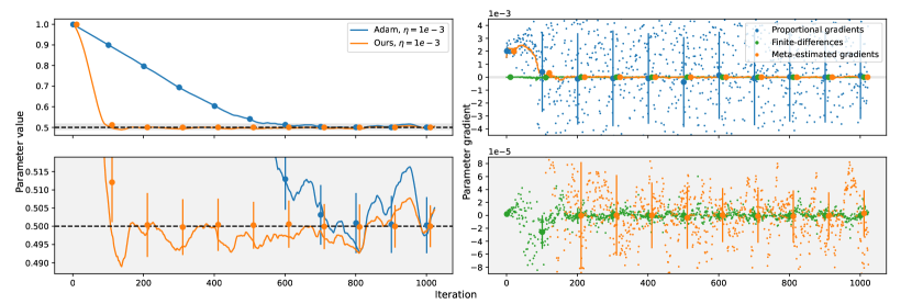
Figure 2. We optimise the rate parameter of an exponential distribution such that the mean of the distribution matches our target value of 2.0. We take 32 samples of the distribution in each iteration and compute an L2 loss between their mean and the target value. The bottom row shows insets of the graphs in the top row, indicated by grey regions. On the left, we show how Adam and our method reach the ground truth rate parameter 0.5. Error bars show the run-to-run variation of the optimised parameter. Our method converges significantly faster and is more stable than Adam. On the right, we show the estimators we use for our method; the proportional estimator has a large variance, while the finite-difference estimator is much less noisy. Our meta-estimator combines both, with its variance reducing over time.

Finite-difference estimation

We write the change of $F_{i}$ between consecutive steps as:

(3) $$\Delta F_{i}=F_{i}-F_{i-1}\text{ .}$$

A finite-difference estimator ($\langle\Delta F_{i}\rangle$) estimates this change, ideally with a low variance. For example, we can substitute Equation 1 into Equation 3:

(4) $$\Delta F_{i}=\int_{\mathcal{X}}f(\mathbf{x},\pi_{i})-f(\mathbf{x},\pi_{i-1})\mathrm{d}\mathbf{x}\text{ ,}$$

and sample with a density $p$ like in Equation 2:

(5) $$\langle\Delta F_{i}\rangle=\frac{f(\mathbf{x},\pi_{i})-f(\mathbf{x},\pi_{i-1})}{p(\mathbf{x},\pi_{i})}\text{ .}$$

Here we assume that $f$ is continuous w.r.t. $\pi_{i}$. Although our theory may apply to any Monte Carlo integral $F_{i}$, we analyse the case where $f(x,\pi_{i})=\partial L/\partial\pi_{i}$ is the gradient at the $i$-th iteration, for some objective $L$.

3.1. Meta-estimation

Our meta-estimator aims to optimally combine each proportional $\langle F_{i}\rangle$ and finite-difference estimator $\langle\Delta F_{i}\rangle$ available until the current step $i$. In this subsection, we establish the theoretical conditions required for a variance-optimal, unbiased combination of both estimators.

A finite-difference estimator $\langle\Delta F_{i}\rangle$, by its definition in Equation 3, lets us update any proportional estimator from the previous step ($\langle F_{i-1}\rangle$) to the current step $i$. This update can be done simply by addition without introducing any bias. We can easily show this by expanding the expected value of the sum:

(6) $$\mathop{\mathbb{E}}[\langle F_{i-1}\rangle+\langle\Delta F_{i}\rangle]=\\ \mathop{\mathbb{E}}[\langle F_{i-1}\rangle]+\mathop{\mathbb{E}}[\langle\Delta F_{i}\rangle]=F_{i-1}+F_{i}-F_{i-1}=F_{i}\text{ .}$$

We define our meta estimator as a weighted sum over the combination of all previous estimators up until step $i$-1 i.e., $\langle F_{i-1}\rangle_{M}$ and the current proportional and finite-difference estimators:

(7) $$\boxed{\langle F_{i}\rangle_{M}=\alpha_{i}(\langle F_{i-1}\rangle_{M}+\langle\Delta F_{i}\rangle)+(1-\alpha_{i})\langle F_{i}\rangle\text{ .}}$$

We initialise $\langle F_{0}\rangle_{M}=\langle F_{0}\rangle$. As we sample all $\langle F_{i}\rangle$ and $\langle\Delta F_{i}\rangle$ independently, the optimal $\alpha_{i}$ coefficients are given by inverse variance weighting (Sinha et al., 2011):

(8) $$\alpha_{i}=\frac{\text{Var}[\langle F_{i}\rangle]}{\text{Var}[\langle F_{i}\rangle]+\text{Var}[\langle F_{i-1}\rangle_{M}]+\text{Var}[\langle\Delta F_{i}\rangle]}\text{ .}$$

This simple recurrent relation captures the variance optimal combination of all previously sampled proportional and finite-difference estimators.

To summarise, we introduce the optimal and unbiased meta-estimator in Equation 7. However, in practice, we use a more efficient implementation which suffers from some start-up bias. We describe this version in the following section. To visualise the estimators mentioned above and to motivate the design of our optimiser, we show a simple example in Figure 2.

4. Variance estimation

Implementing Equation 7 in practice presents a challenge due to the unknown variances of our estimators. In this section, we describe how we approximate each variance term. We must balance three main objectives: the efficiency of our variance approximation methods, the optimality of our approximated $\alpha_{i}$ coefficients, and any bias potentially introduced to $\langle F_{i}\rangle_{M}$.

4.1. Proportional estimator variance

We approximate $\text{Var}[\langle F_{i}\rangle]$ as a zero-centred raw moment (Papoulis and Pillai, 1984), computed using an exponential moving average (EMA) with coefficient $\beta_{F}$:

(9) $$\text{Var}[\langle F_{i}\rangle]=\beta_{F}\,\text{Var}[\langle F_{i-1}\rangle]+(1-\beta_{F})\langle F_{i}\rangle^{2}\text{ .}$$

This formulation is similar to Adam’s second moment estimate (Kingma and Ba, 2014). Here, $\text{Var}[\langle F_{i}\rangle]$ is a large, stable value that only varies in the initial stage of optimisation, when parameter changes can notably affect the problem’s overall noise characteristics. A large $\beta_{F}$ coefficient minimises the correlation of the approximate variance to any singular $\langle F_{i}\rangle$, resulting in an overall stable variance approximation.

4.2. Finite-difference estimator variance

As the proportional estimator reaches steady-state, we can safely assume that $\langle F_{i}\rangle$ are identically distributed over consecutive iterations. Unfortunately, the same observation does not apply to finite-difference estimation as this finite-difference depends on the optimisation step we take in the previous iteration. For example, a larger step will cause a larger shift in the per-parameter gradients.

To resolve this issue we propose to decouple the optimisation step size ($|\Delta\pi_{i}|$) from the approximated finite-difference estimator variance ($\text{Var}[\langle\Delta F_{i}\rangle]$). We begin the derivation of this decoupling by expanding the fraction in Equation 5 by the Euclidean step size $||\Delta\pi_{i}||_{2}$ of the previous iteration:

(10) $$\langle\Delta F_{i}\rangle=\frac{f(\mathbf{x},\pi_{i})-f(\mathbf{x},\pi_{i-1})}{p(\mathbf{x},\pi_{i})}=\frac{f(\mathbf{x},\pi_{i})-f(\mathbf{x},\pi_{i-1})}{||\Delta\pi_{i}||_{2}p(\mathbf{x},\pi_{i})}||\Delta\pi_{i}||_{2}\,.$$

For sufficiently small step sizes, we can rearrange the terms in Equation 10 to approximate the finite-difference of gradients $f$ as the second-order gradient ($\partial f/\partial\pi$), times a unit-directional vector, times the left over terms:

(11) $$\langle\Delta F_{i}\rangle\approx\left(\frac{\partial f}{\partial\pi}(\mathbf{x},\pi_{i})\cdot\frac{\Delta\pi_{i}}{||\Delta\pi_{i}||_{2}}\right)\frac{||\Delta\pi_{i}||_{2}}{p(\mathbf{x},\pi_{i})}\text{ .}$$

Applying the variance operator to Equation 11 gives us the decoupled finite-difference variance ($\text{Var}[\langle\Delta F_{i}\rangle]_{D}$):

(12) $$\text{Var}[\langle\Delta F_{i}\rangle]\approx\text{Var}\left[\left(\frac{\partial f}{\partial\pi}(\mathbf{x},\pi_{i})\cdot\frac{\Delta\pi_{i}}{||\Delta\pi_{i}||_{2}}\right)\frac{1}{p(\mathbf{x},\pi_{i})}\right]||\Delta\pi||_{2}^{2}\\ =\text{Var}[\langle\Delta F_{i}\rangle]_{D}||\Delta\pi||_{2}^{2}\text{ .}$$

We use a zero-centred EMA, with a coefficient $\beta_{\Delta}$, to approximate this decoupled variance as:

(13) $$\text{Var}[\langle\Delta F_{i}\rangle]_{D}=\beta_{\Delta}\,\text{Var}[\langle\Delta F_{i-1}\rangle]_{D}+(1-\beta_{\Delta})\frac{\langle\Delta F_{i}\rangle^{2}}{||\Delta\pi||_{2}^{2}}\text{ .}$$

We generally use a small $\beta_{\Delta}$ coefficient as $\text{Var}[\langle\Delta F_{i}\rangle]_{D}$ can change quickly and is typically less noisy than $\text{Var}[\langle F_{i}\rangle]$. Finally, we can rescale $\text{Var}[\langle\Delta F_{i}\rangle]_{D}$ to estimate $\text{Var}[\langle\Delta F_{i}\rangle]$:

(14) $$\text{Var}[\langle\Delta F_{i}\rangle]=\text{Var}[\langle\Delta F_{i}\rangle]_{D}\,||\Delta\pi||_{2}^{2}\text{ .}$$

We found this decoupled variance more closely distributed between iterations, better suited for approximation via moving averages.

4.3. Meta-estimator variance

We approximate the variance of our meta estimator in Equation 7 by recurrently applying the variance operator:

(15) $$\text{Var}[\langle F_{i}\rangle_{M}]=\alpha_{i}^{2}(\text{Var}[\langle F_{i-1}\rangle_{M}]+\text{Var}[\langle\Delta F_{i}\rangle])\\ +(1-\alpha_{i})^{2}\text{Var}[\langle F_{i}\rangle]\text{ .}$$

Here we assume $\alpha_{i}$ to be a non-random value to simplify our mathematical derivation. Later in Section 6, we show the choice of $\alpha_{i}$ is less significant as long as its correlation with the gradient samples diminishes.

4.4. Alpha clipping

Meta-estimation is most vulnerable to underestimated $\text{Var}[\langle F_{i}\rangle_{M}]$; unless a significant $\text{Var}[\langle\Delta F_{i}\rangle]$ indicates a shift, $\langle F_{i}\rangle_{M}$ will only slowly correct its overconfidently estimated value by averaging $\langle F_{i}\rangle$ over many iterations. The risk of underestimation is the greatest while our exponential moving averages accumulate their initial samples. Clipping alpha based on the iteration resolves this risk:

(16) $$\alpha_{i}=\min(\alpha_{i},1-1/(i+1))\text{ .}$$

Intuitively, Equation 16 constrains alpha by the perfect average of all previous estimates; any value above this must be overestimated. We generalise this observation to the entire optimisation process, assuming that $\text{Var}[\langle F_{i}\rangle]$ is similar in subsequent steps:

(17) $$\alpha_{i}=\min(\alpha_{i},1/(2-\alpha_{i-1}))\text{ .}$$

5. Optimisation

Combining meta-estimation and optimisation creates a complex feedback loop; the meta-estimated gradients $\langle F_{i}\rangle_{M}$ depend on their finite-difference estimates $\langle\Delta F_{i}\rangle$, which depend on the optimiser’s steps $\Delta\pi_{i}$, which, in turn, depend on the gradients estimated in the previous step $\langle F_{i-1}\rangle_{M}$. It becomes crucial that the meta-estimator provides the optimiser with reliable gradients and that the optimiser makes steps that let the meta-estimator converge. We aim to combine Adam with meta-estimated gradients. We explain Adam’s variance approximation and update rule to show where we can integrate meta-estimation.

Adam (Kingma and Ba, 2014) is well known for its robustness to outlier gradient samples; upon encountering an outlier, the estimated second moments adjust in the same step, swiftly pulling down the step size. This mechanism works because Adam first updates its second-moment estimate:

(18) $$v_{i}=\beta_{2}v_{i-1}+(1-\beta_{2})\langle F_{i}\rangle^{2}\text{ ,}$$

corrects the EMA startup bias:

(19) $$\hat{v_{i}}=v_{i}/(1-\beta_{2}^{i})\text{ ,}$$

and then divides the step size by its square root:

(20) $$\Delta\pi_{i+1}=-\eta\frac{\hat{m_{i}}}{\sqrt{\hat{v_{i}}}+\epsilon}\text{ ,}$$

where $m_{i}$ and $v_{i}$ refer to Adam’s moment estimates, $\eta$ to the learning rate, $\beta_{2}$ to Adam’s second moment coefficient, and $\epsilon$ to a small value to ensure numerical stability. $\alpha_{i}$ and $\text{Var}[\langle F_{i}\rangle]$ behave similarly in our case; first, we update $\text{Var}[\langle F_{i}\rangle]$ for the current step (Equation 9), compute $\alpha_{i}$ (Equation 8), and add the outlier gradient $\langle F_{i}\rangle$ to our meta-estimator $\langle F_{i}\rangle_{M}$ weighted by $(1-\alpha_{i})$ (Equation 7). Therefore, just like $\beta_{2}$ for Adam, $\beta_{F}$ offers a tradeoff between outlier robustness and estimation bias.

When using optimisers like RMSProp (Graves, 2014) and Adam (Kingma and Ba, 2014), lower variance gradients naturally accelerate convergence since these optimisers divide their step size by the standard deviation of the gradients (Equation 20). Additionally, Momentum (Sutskever et al., 2013) helps these optimisers handle tricky non-linear, multivariate curvatures such as ravines. The optimisers’ effectiveness is greatly reduced if the noise in the gradients overpowers the variance arising from non-linearities in the estimated moments required for these mechanisms.

Naively feeding the meta-estimated gradients to Adam is problematic; Adam computes its moment estimates, assuming the input gradients in each iteration to be independent. Meanwhile, our meta-estimator outputs an already averaged gradient (Equation 7) with a strong positive correlation to previous averages. Adam’s moment estimates are also redundant since we already estimate the variance of our meta-estimator $\text{Var}[\langle F_{i}\rangle_{M}]$. Therefore, we formulate the update step in terms of our estimates:

(21) $$\Delta\pi_{i+1}=-\eta\frac{\langle F_{i}\rangle_{M}}{\sqrt{\text{Var}[\langle F_{i}\rangle_{M}]}+\epsilon}\text{ .}$$

Dividing by $\sqrt{\text{Var}[\langle F_{i}\rangle_{M}]}$ sets the step size based on our meta-estimator. As $\text{Var}[\langle F_{i}\rangle_{M}]$ responds to changes in the estimated gradients much more quickly than Adam’s second-moment estimate with the suggested $\beta_{2}=0.999$ parameter, the stability of our method may seem uncertain. We observe that the responsivity of our method actually improves convergence, especially when combined with the decoupled estimation of $\text{Var}[\langle\Delta F_{i}\rangle]$. Optimisation speeds up quickly when low-noise gradients are available and slows down naturally when approaching a minimum.

6. Experiments

We run several experiments to confirm our method’s behaviour and verify its theory. We also compare our method against Adam, as it is used in state-of-the-art inverse rendering pipelines. We implement our method in Mitsuba 3 (Jakob et al., 2022) and use Path Replay Backpropagation (Vicini et al., 2021) to sample gradients computed with the unbiased Mean Relative Squared Error loss (Deng et al., 2022; Pidhorskyi et al., 2022). For texture optimisation tasks, we use gradient preconditioning as proposed by Nicolet et al. (2021). We compute $\langle\Delta F_{i}\rangle$ with a simplified form of the shift mapping proposed by Kettunen et al. (2015), only accounting for the BRDF sampling. While this implementation is sufficient for our proof-of-concept demonstrations, a full implementation of shift mapping can also account for changes in geometry at an insignificant cost compared to proportional samples. Unless mentioned otherwise, we tune learning rates of each method in each experiment.

Variance reduction without lag

We investigate the variance reduction our method can achieve while the scene parameters are changing. We run a fixed linear interpolation of the parameters without an optimiser to prevent any effects from the feedback of the gradients.

Forward gradients of several pixels in Figure 3 show that our method avoids the lag in gradients typical of EMAs. Our meta-estimate’s actual variances and estimate variances are much tighter than the estimates computed by Adam. Furthermore, our method remains more stable upon encountering outliers.

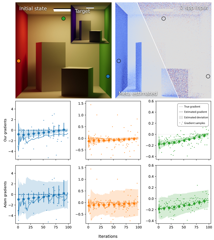
Figure 3. We estimate forward gradients of the left wall’s colour’s blue channel while linearly changing the scene from the initial state (top left) to the target state over 100 iterations. The dashed line represents the actual gradient, dots the gradient samples, the solid line the estimated gradient, and the shaded area the estimated standard deviation. Error bars every 10 iterations show the run-to-run variation of the estimated gradient. Meta-estimation eliminates lag, improves robustness to outliers, and offers lower variance while more accurately estimating this variance. We select the three pixels w.r.t. the actual gradient variance; blue is the noisiest, orange is at 75’th percentile, and green is the median.

Approximation accuracy

We repeat the previous setup in Figure 4, only now we test an exponentially decaying change in the gradients. Again, our meta-estimator stays within 0.5 to 2 times its predicted standard deviation. As the gradients settle, our method provides a consistent variance reduction (Row 1), averaging a large number of samples wherever possible. Meanwhile, Adam struggles with high-variance gradients (Row 2) and is thrown off by outliers.

We also show the approximated variances compared to ground truth variances computed over 1000 independent runs. Our approximation methods perform reasonably, only overestimating $\text{Var}[\langle F_{i}\rangle]$ (Row 3). This overestimation results in generally conservative $\alpha_{i}$ values, erring on the side of robustness rather than maximising variance reduction (Row 5). On the other hand, we approximate $\text{Var}[\langle\Delta F_{i}\rangle]$ (Row 4) with little bias, although with often a large run-to-run variance.

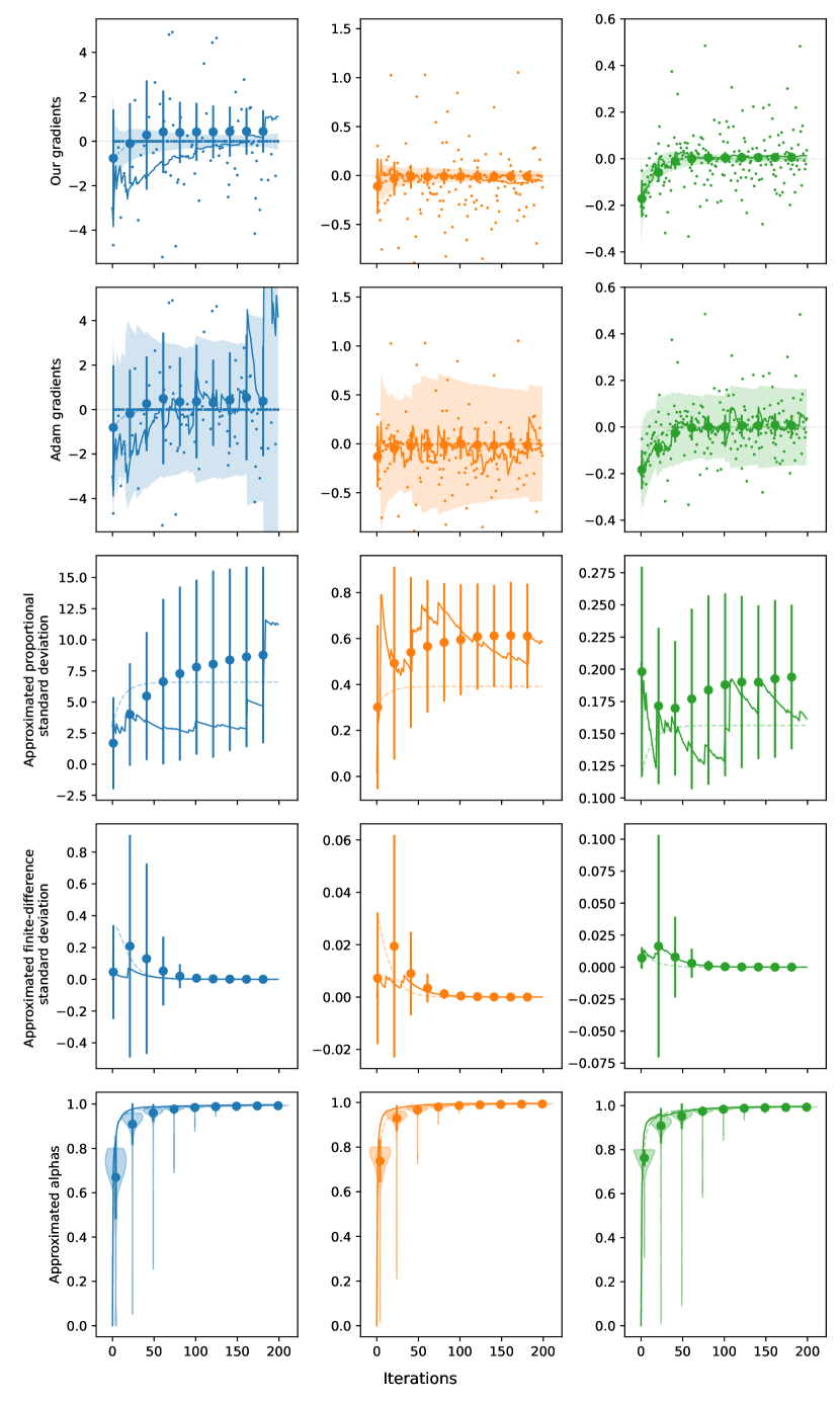
Figure 4. Following the same setup as Figure 3, we show the estimated gradients and standard deviations of our meta-estimator and Adam. Our meta-estimators achieve significantly lower actual variance in each case, while also providing much more accurate approximations. Dashed lines represent actual or optimal values, solid lines a randomly sampled run, while error bars show run-to-run variation. In addition, we show violin plots for alpha, demonstrating how our method is more likely to be conservative and not to be swayed by outliers.

Multivariate optimisation

We simultaneously optimise an object’s colour, metalness, and roughness, as shown in Figure 1. Thanks to our meta-estimator, our method can traverse the loss surface without losing past samples. Furthermore, our finite-difference estimates let our meta-estimator adjust rapidly, avoiding the overshoots typical of Momentum-based methods. Even when tuning Adam’s hyperparameters for the specific problem, it can only match our method at an over 20 times increase in computational cost, not counting the time spent on hyperparameter tuning.

Texture optimisation

We show a difficult texture optimisation case in Figure 6. Texture optimisation requires disentangling global illumination with very few gradient samples per texel. Adam can only take a few steps within a fixed budget at a high sample count, requiring a high learning rate that skips over the intricate loss surface necessary to navigate for disentangling various effects. At a lower sample count, however, Adam struggles to progress as steps devolve into a random walk as the scale of the gradients shrinks close to minima.

High-dimensional optimisation

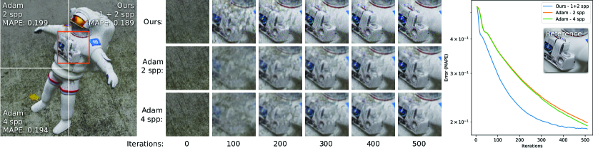
Figure 7. We optimise emission and absorption volumes in a NeRF-like experiment. Regarding computational cost, our method lies between 2 spp and 4 spp Adam at one finite-difference and two proportional samples. However, we greatly outperform both regarding convergence and final quality. Although the final quantitative difference is smaller, we resolve jarring artefacts such as holes in the volume and overall blur. Astronaut © 2023 jgilhutton

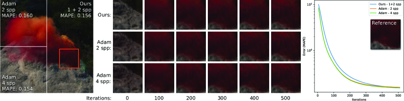
Figure 8. Same setup as Figure 7. Our method performs worse here as the volume is sparser, concentrating our finite-difference samples less. Thus, parameters at individual voxels are samples relatively sparsely, making finite-difference estimation for the whole volume difficult. Smoke © 2023 JangaFX Software

In Figure 7, we optimise an emissive-absorptive volume of size 256$\times$256$\times$256 voxels, totalling 70 million parameters. Perfectly fitting such a non-physical volume to rendered images is impossible. Thus, the optimiser needs to balance per-pixel losses for a good approximation, further needing to disentangle the small subset of parameters visible through any given pixel. Previous works avoid convergence to local minima by upsampling the optimised volume in several stages; our method does not need this workaround. On the other hand, Figure 8 shows that our method provides less benefit when our finite-difference estimator’s sampling is too sparse across the volume.

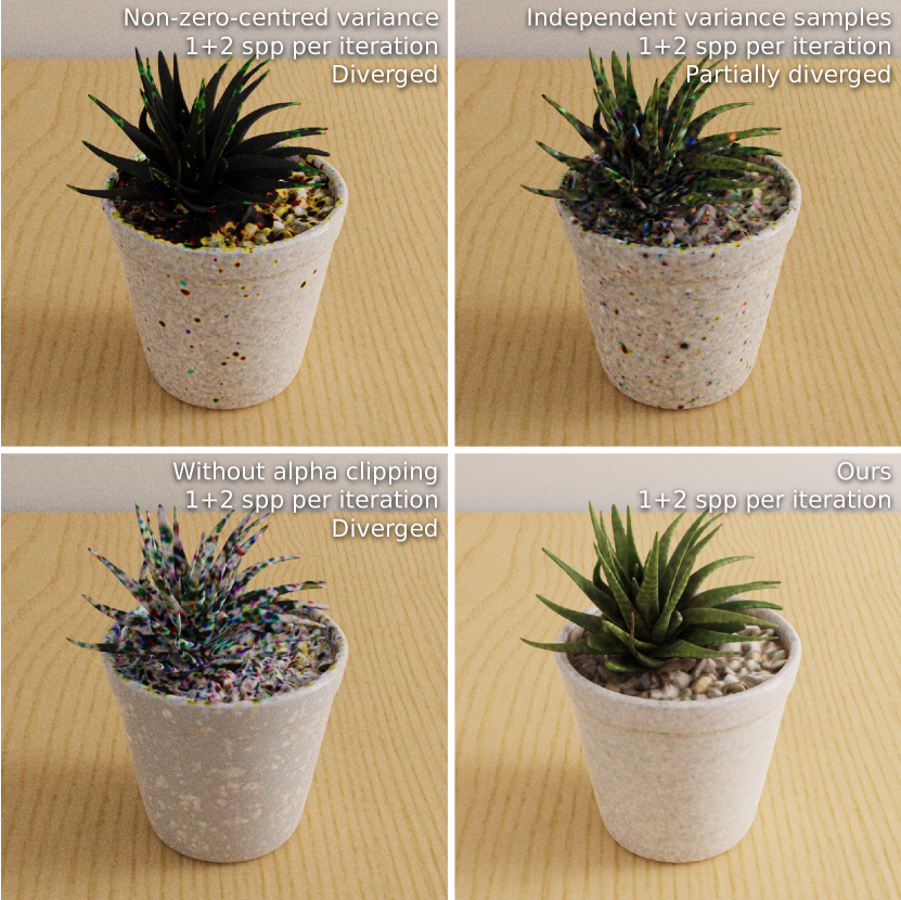
Figure 5. We ablate our design choices, demonstrating their importance for robust gradient estimation and optimisation. Each modification of our method is less robust than our results in Figure 6. Potted Plant © 2023 James Ray Cock

Zero-centred EMAs

We chose to use zero-centred moving averages so that we do not need to approximate the mean of our estimators directly. This approach is generally more robust and memory efficient, though it overestimates variance at large signal-to-noise ratios. However, gradients generally have a low signal-to-noise ratio, so this tradeoff works in our favour. Figure 5 (top-left) demonstrates how non-zero-centred variance approximation is unstable, providing unreliable alphas, thus causing optimisation to diverge.

Alpha clipping

Alpha clipping helps resolve cases when our approximated variances are inaccurate, improving robustness. It may hinder the variance reduction of our method in the special case when $\text{Var}[\langle F_{i}\rangle]$ is sharply decreasing over iterations. However, we have not encountered this behaviour with our tested proportional estimators. Figure 5 (bottom-left) shows an ablation without alpha clipping for a scene from Figure 6, demonstrating rapid divergence as the initial variance approximations are unreliable.

Sample reuse

We use the same samples for rendering and variance approximation. This correlation introduces some bias at the start of the optimisation process, which diminishes over time. Figure 5 (top-right) shows an unbiased ablation using uncorrelated samples. Although this independently approximated variance eliminates bias, it misses outliers in the samples used for gradient estimation, causing the parameters receiving these outliers to diverge.

7. Limitations

Estimators $\langle\Delta F_{i}\rangle$ are not generally available for many problems. Kettunen et al. (2015) propose shift mapping for path tracing, which we use in our work. Our meta-estimators rely heavily on $\langle\Delta F_{i}\rangle$; as we recurrently sum $\text{Var}[\langle\Delta F_{i}\rangle]$ in Equation 15, it inherently bounds the variance of our meta-estimator. Doing so is fine as long as $\text{Var}[\langle\Delta F_{i}\rangle]$ is quadratic w.r.t. the step size (Equation 14). Thus, we need to ensure this property when building finite-difference estimators while also aiming for the lowest variance to achieve the best stability and convergence with meta-estimation.

Zeltner et al. (2021) show that gradient estimators benefit from specialised differential sampling strategies. The same is true of finite-difference estimators; our naive toy formulation in Equation 5 glosses over this problem where $p(\mathbf{x},\pi_{i})$ is usually only optimised by importance sampling $f(\mathbf{x},\pi_{i})$, not the difference between $f(\mathbf{x},\pi_{i})$ and $f(\mathbf{x},\pi_{i-1})$.

Suboptimal sampling strategies of $\langle F_{i}\rangle$ compound the issue. As our work focuses on gradient estimation, meaning $F_{i}$ are gradients, sampling of $\langle F_{i}\rangle$ is not yet well established. For example, Zeltner et al. (2021) show the poor performance of roughness gradient estimators. We experience these issues first-hand, as we show in Figure 9.

8. Conclusion

Our proposed meta-estimation technique and corresponding adaptation of the Adam update rule can substantially improve convergence when descending on noisy gradients, reducing computation costs by several orders of magnitude. We solve cases where low-sample-count gradients are too noisy for fast convergence while high-sample-count gradients are prohibitively expensive to compute for the required number of iterations on difficult non-linear, multivariate problems.

Future work

We look forward to applications of meta-estimation to various inverse Monte Carlo problems, especially as MC gradient estimators become prominent in machine learning (Mohamed et al., 2020). Building good gradient and finite-difference estimators may seem challenging — and are the main limitation of our method — but it is undoubtedly a fruitful direction for future work. We did not investigate training deep neural networks in this work but see it as the next step once low-variance finite-difference estimators become available.

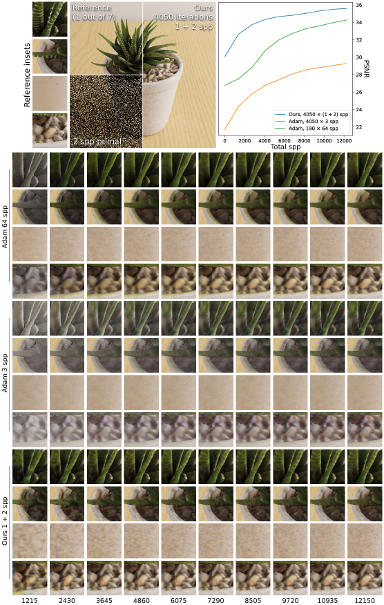
Figure 6. We optimise diffuse textures, placing a potted plant in the extremely noisy Veach Ajar scene. At 64 spp, Adam can only afford to take a few steps at a large learning rate and cannot match small details, further failing on complex interactions such as the leaf’s reflection on the pot’s side, where navigating a difficult loss surface is necessary. At 3 spp, Adam reduces to a random walk after reaching vaguely accurate parameters where gradients vanish against the high noise level. Our estimator shows good convergence. Textures remain a little blurry as a known consequence of regularisation (Nicolet et al., 2021). The texture of the glossy pot (third inset) shows relatively worse convergence due to the concerns discussed in Section 7. Potted Plant © 2023 James Ray Cock, Veach Ajar © 2023 Benedikt Bitterli

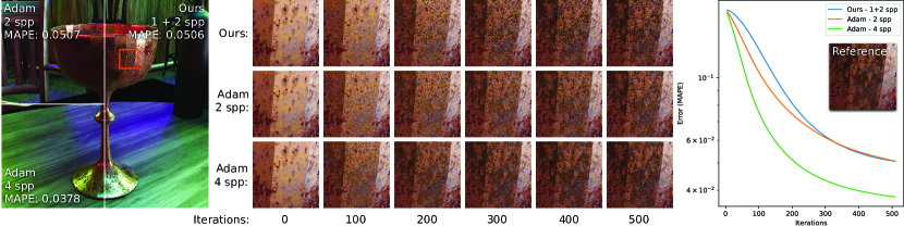
Figure 9. We optimise the 2K roughness texture of the Chalice scene from Chang et al. (2023). Using only basic shift mapping, our finite-difference estimator struggles to cope with the changes in roughness over sharp lighting. As the roughness parameter influences our sampling strategy, this is a challenging case for finite-difference estimation. Chalice © 2023 SusanKing

- (1)
- Bangaru et al. (2020) Sai Praveen Bangaru, Tzu-Mao Li, and Frédo Durand. 2020. Unbiased Warped-Area Sampling for Differentiable Rendering. ACM Trans. Graph. 39, 6, Article 245 (nov 2020), 18 pages. https://doi.org/10.1145/3414685.3417833
- Bitterli et al. (2020) Benedikt Bitterli, Chris Wyman, Matt Pharr, Peter Shirley, Aaron Lefohn, and Wojciech Jarosz. 2020. Spatiotemporal reservoir resampling for real-time ray tracing with dynamic direct lighting. ACM Transactions on Graphics (Proceedings of SIGGRAPH) 39, 4 (July 2020). https://doi.org/10/gg8xc7
- Chang et al. (2023) Wesley Chang, Venkataram Sivaram, Derek Nowrouzezahrai, Toshiya Hachisuka, Ravi Ramamoorthi, and Tzu-Mao Li. 2023. Parameter-Space ReSTIR for Differentiable and Inverse Rendering. In ACM SIGGRAPH 2023 Conference Proceedings (Los Angeles, CA, USA) (SIGGRAPH ’23). Association for Computing Machinery, New York, NY, USA, Article 18, 10 pages. https://doi.org/10.1145/3588432.3591512
- Defazio et al. (2014) Aaron Defazio, Francis Bach, and Simon Lacoste-Julien. 2014. SAGA: A Fast Incremental Gradient Method With Support for Non-Strongly Convex Composite Objectives. In Advances in Neural Information Processing Systems, Z. Ghahramani, M. Welling, C. Cortes, N. Lawrence, and K.Q. Weinberger (Eds.), Vol. 27. Curran Associates, Inc. https://proceedings.neurips.cc/paper_files/paper/2014/file/ede7e2b6d13a41ddf9f4bdef84fdc737-Paper.pdf
- Deng et al. (2022) Xi Deng, Fujun Luan, Bruce Walter, Kavita Bala, and Steve Marschner. 2022. Reconstructing Translucent Objects Using Differentiable Rendering. In ACM SIGGRAPH 2022 Conference Proceedings (Vancouver, BC, Canada) (SIGGRAPH ’22). Association for Computing Machinery, New York, NY, USA, Article 38, 10 pages. https://doi.org/10.1145/3528233.3530714
- Fieller and Hartley (1954) EC Fieller and HO Hartley. 1954. Sampling with control variables. Biometrika 41, 3/4 (1954), 494–501.
- Gower et al. (2020) Robert M. Gower, Mark Schmidt, Francis Bach, and Peter Richtárik. 2020. Variance-Reduced Methods for Machine Learning. Proc. IEEE 108, 11 (2020), 1968–1983. https://doi.org/10.1109/JPROC.2020.3028013
- Graves (2014) Alex Graves. 2014. Generating Sequences With Recurrent Neural Networks. arXiv:1308.0850 [cs.NE]
- Igehy (1999) Homan Igehy. 1999. Tracing Ray Differentials. In Proceedings of the 26th Annual Conference on Computer Graphics and Interactive Techniques (SIGGRAPH ’99). ACM Press/Addison-Wesley Publishing Co., USA, 179–186. https://doi.org/10.1145/311535.311555
- Jakob et al. (2022) Wenzel Jakob, Sébastien Speierer, Nicolas Roussel, Merlin Nimier-David, Delio Vicini, Tizian Zeltner, Baptiste Nicolet, Miguel Crespo, Vincent Leroy, and Ziyi Zhang. 2022. Mitsuba 3 renderer. https://mitsuba-renderer.org.
- Johnson and Zhang (2013) Rie Johnson and Tong Zhang. 2013. Accelerating Stochastic Gradient Descent using Predictive Variance Reduction. In Advances in Neural Information Processing Systems, C.J. Burges, L. Bottou, M. Welling, Z. Ghahramani, and K.Q. Weinberger (Eds.), Vol. 26. Curran Associates, Inc. https://proceedings.neurips.cc/paper_files/paper/2013/file/ac1dd209cbcc5e5d1c6e28598e8cbbe8-Paper.pdf
- Kajiya (1986) James T Kajiya. 1986. The rendering equation. In Proceedings of the 13th annual conference on Computer graphics and interactive techniques. 143–150.
- Kalman (1960) R. E. Kalman. 1960. A New Approach to Linear Filtering and Prediction Problems. Journal of Basic Engineering 82, 1 (03 1960), 35–45. https://doi.org/10.1115/1.3662552 arXiv:https://asmedigitalcollection.asme.org/fluidsengineering/article-pdf/82/1/35/5518977/35_1.pdf
- Kettunen et al. (2015) Markus Kettunen, Marco Manzi, Miika Aittala, Jaakko Lehtinen, Frédo Durand, and Matthias Zwicker. 2015. Gradient-Domain Path Tracing. ACM Trans. Graph. 34, 4, Article 123 (jul 2015), 13 pages. https://doi.org/10.1145/2766997
- Kingma and Ba (2014) Diederik P Kingma and Jimmy Ba. 2014. Adam: A method for stochastic optimization. arXiv preprint arXiv:1412.6980 (2014).
- Lehtinen et al. (2013) Jaakko Lehtinen, Tero Karras, Samuli Laine, Miika Aittala, Frédo Durand, and Timo Aila. 2013. Gradient-Domain Metropolis Light Transport. 32, 4, Article 95 (jul 2013), 12 pages. https://doi.org/10.1145/2461912.2461943
- Li et al. (2018) Tzu-Mao Li, Miika Aittala, Frédo Durand, and Jaakko Lehtinen. 2018. Differentiable Monte Carlo Ray Tracing through Edge Sampling. ACM Trans. Graph. 37, 6, Article 222 (dec 2018), 11 pages. https://doi.org/10.1145/3272127.3275109
- Manzi et al. (2016) Marco Manzi, Markus Kettunen, Frédo Durand, Matthias Zwicker, and Jaakko Lehtinen. 2016. Temporal Gradient-Domain Path Tracing. ACM Trans. Graph. 35, 6, Article 246 (dec 2016), 9 pages. https://doi.org/10.1145/2980179.2980256
- Mohamed et al. (2020) Shakir Mohamed, Mihaela Rosca, Michael Figurnov, and Andriy Mnih. 2020. Monte Carlo Gradient Estimation in Machine Learning. J. Mach. Learn. Res. 21, 1, Article 132 (jan 2020), 62 pages.
- Moulines and Bach (2011) Eric Moulines and Francis Bach. 2011. Non-Asymptotic Analysis of Stochastic Approximation Algorithms for Machine Learning. In Advances in Neural Information Processing Systems, J. Shawe-Taylor, R. Zemel, P. Bartlett, F. Pereira, and K.Q. Weinberger (Eds.), Vol. 24. Curran Associates, Inc. https://proceedings.neurips.cc/paper_files/paper/2011/file/40008b9a5380fcacce3976bf7c08af5b-Paper.pdf
- Nesterov (1983) Yurii Evgen’evich Nesterov. 1983. A method of solving a convex programming problem with convergence rate Obigl(k^2bigr). In Doklady Akademii Nauk, Vol. 269. Russian Academy of Sciences, 543–547.
- Nicolet et al. (2021) Baptiste Nicolet, Alec Jacobson, and Wenzel Jakob. 2021. Large Steps in Inverse Rendering of Geometry. ACM Trans. Graph. 40, 6, Article 248 (dec 2021), 13 pages. https://doi.org/10.1145/3478513.3480501
- Nicolet et al. (2023) Baptiste Nicolet, Fabrice Rousselle, Jan Novák, Alexander Keller, Wenzel Jakob, and Thomas Müller. 2023. Recursive Control Variates for Inverse Rendering. Transactions on Graphics (Proceedings of SIGGRAPH) 42, 4 (Aug. 2023). https://doi.org/10.1145/3592139
- Nimier-David et al. (2020) Merlin Nimier-David, Sébastien Speierer, Benoît Ruiz, and Wenzel Jakob. 2020. Radiative Backpropagation: An Adjoint Method for Lightning-Fast Differentiable Rendering. Transactions on Graphics (Proceedings of SIGGRAPH) 39, 4 (July 2020). https://doi.org/10.1145/3386569.3392406
- Owen (2013) Art B Owen. 2013. Monte Carlo theory, methods and examples. (2013).
- Papoulis and Pillai (1984) Athanasios Papoulis and S Unnikrishna Pillai. 1984. Probability, random variables, and stochastic processes. McGraw-Hill, 145–149.
- Pharr et al. (2016) Matt Pharr, Wenzel Jakob, and Greg Humphreys. 2016. Physically Based Rendering: From Theory to Implementation (3rd ed.) (3rd ed.). Morgan Kaufmann Publishers Inc., San Francisco, CA, USA.
- Pidhorskyi et al. (2022) Stanislav Pidhorskyi, Timur Bagautdinov, Shugao Ma, Jason Saragih, Gabriel Schwartz, Yaser Sheikh, and Tomas Simon. 2022. Depth of Field Aware Differentiable Rendering. 41, 6, Article 190 (nov 2022), 18 pages. https://doi.org/10.1145/3550454.3555521
- Polyak and Juditsky (1992) Boris T Polyak and Anatoli B Juditsky. 1992. Acceleration of stochastic approximation by averaging. SIAM journal on control and optimization 30, 4 (1992), 838–855.
- Rousselle et al. (2016) Fabrice Rousselle, Wojciech Jarosz, and Jan Novák. 2016. Image-Space Control Variates for Rendering. ACM Trans. Graph. 35, 6, Article 169 (dec 2016), 12 pages. https://doi.org/10.1145/2980179.2982443
- Sinha et al. (2011) Bimal K Sinha, Joachim Hartung, and Guido Knapp. 2011. Statistical meta-analysis with applications. John Wiley & Sons.
- Smith et al. (2018) Samuel L. Smith, Pieter-Jan Kindermans, Chris Ying, and Quoc V. Le. 2018. Don’t Decay the Learning Rate, Increase the Batch Size. arXiv:1711.00489 [cs.LG]
- Sutskever et al. (2013) Ilya Sutskever, James Martens, George Dahl, and Geoffrey Hinton. 2013. On the importance of initialization and momentum in deep learning. In International conference on machine learning. PMLR, 1139–1147.
- Vicini et al. (2021) Delio Vicini, Sébastien Speierer, and Wenzel Jakob. 2021. Path Replay Backpropagation: Differentiating Light Paths using Constant Memory and Linear Time. Transactions on Graphics (Proceedings of SIGGRAPH) 40, 4 (Aug. 2021), 108:1–108:14. https://doi.org/10.1145/3450626.3459804
- Yan et al. (2022) Kai Yan, Christoph Lassner, Brian Budge, Zhao Dong, and Shuang Zhao. 2022. Efficient Estimation of Boundary Integrals for Path-Space Differentiable Rendering. ACM Trans. Graph. 41, 4, Article 123 (jul 2022), 13 pages. https://doi.org/10.1145/3528223.3530080
- Zeltner et al. (2021) Tizian Zeltner, Sébastien Speierer, Iliyan Georgiev, and Wenzel Jakob. 2021. Monte Carlo Estimators for Differential Light Transport. Transactions on Graphics (Proceedings of SIGGRAPH) 40, 4 (Aug. 2021). https://doi.org/10.1145/3450626.3459807
- Zhang et al. (2021) Cheng Zhang, Zhao Dong, Michael Doggett, and Shuang Zhao. 2021. Antithetic Sampling for Monte Carlo Differentiable Rendering. ACM Trans. Graph. 40, 4 (2021), 77:1–77:12.
- Zhang et al. (2020) Cheng Zhang, Bailey Miller, Kai Yan, Ioannis Gkioulekas, and Shuang Zhao. 2020. Path-Space Differentiable Rendering. ACM Trans. Graph. 39, 4, Article 143 (aug 2020), 19 pages. https://doi.org/10.1145/3386569.3392383
- Zhang et al. (2019) Cheng Zhang, Lifan Wu, Changxi Zheng, Ioannis Gkioulekas, Ravi Ramamoorthi, and Shuang Zhao. 2019. A Differential Theory of Radiative Transfer. ACM Trans. Graph. 38, 6, Article 227 (nov 2019), 16 pages. https://doi.org/10.1145/3355089.3356522