Quantum autoencoders using mixed reference states

Abstract

One of the fundamental tasks in information theory is the compression of information. To achieve this in the quantum domain, quantum autoencoders that aim to compress quantum states to low-dimensional ones have been proposed. When taking a pure state as the reference state, there exists an upper bound for the encoding fidelity. This bound limits the compression rate for high-rank states that have high entropy. To overcome the entropy inconsistency between the initial states and the reconstructed states, we allow the reference state to be a mixed state. A new cost function that combines the encoding fidelity and the quantum mutual information is proposed for compressing general input states. In particular, we consider the reference states to be a mixture of maximally mixed states and pure states. To achieve efficient compression for different states, two strategies for setting the ratio of mixedness (in the mixture of maximally mixed states and pure states) are provided based on prior knowledge about quantum states or observations obtained from the training process. Numerical results on thermal states of the transverse-field Ising model, Werner states, and maximally mixed states blended with pure states illustrate the effectiveness of the proposed method. In addition, quantum autoencoders using mixed reference states are experimentally implemented on IBM Quantum devices to compress and reconstruct thermal states and Werner states.

I Introduction

Quantum machine learning which combines machine learning and quantum computation has grown into a booming research topic biamonte2017quantum ; dong2008quantum ; huang2021power ; cerezo2022challenges ; niu2019universal ; li2020quantum ; dong2022quantum . Quantum autoencoders (QAEs) inherit the spirit of classical autoencoders that compress information into a latent space such that the input can be reconstructed from a reduced-dimension representation pu2016variational ; bartuuvskova2006optical . They have the potential to reduce the requirements of quantum communication channels steinbrecher2019quantum and the size of quantum gates lamata2018quantum ; ding2019experimental and thus have a practical value for various applications including quantum simulation aspuru2005simulated , quantum communication and distributed computation in quantum networks steinbrecher2019quantum ; lamata2018quantum .

Owing to the potential of QAEs in quantum information processing, there is a growing interest in designing different schemes to complete state compression tasks. An early work proposed a quantum generalization of a classical neural network wan2017quantum and another work designed an autoencoder framework using programmable circuits and applied it to reconstruct the ground states of Hubbard models, and molecular Hamiltonians romero2017quantum . An enhanced feature quantum autoencoder that encodes the feature vector of the input data into every single-qubit rotation gate has been implemented in variational quantum circuits bravo2021quantum . There have also been achievements in the implementation of QAEs on photonic systems pepper2019experimental ; huang2020realization ; ding2019experimental . Specifically, a quantum optical neural network has been integrated into a QAE to compress quantum optical states ding2019experimental . QAE based on the control of a photonic device has been implemented to compress qutrits to qubits pepper2019experimental and 2-qubit states into 1-qubit states huang2020realization . Apart from data compression, QAE has also been applied to other applications. The potential of QAE in denoising Greenberger-Horne-Zeilinger states has been investigated bondarenko2020quantum ; achache2020denoising . QAE has also been utilized for error mitigation zhang2021generic . A novel method based on QAE has been devised to prepare the quantum Gibbs state and estimate the quantum Fisher information du2021exploring . A hybrid quantum autoencoder has been proposed to identify the emergence of order in the latent space that can be utilized for clustering and semi-supervised classification srikumar2021clustering . Recently, the execution of a quantum-autoencoder facilitated teleportation protocol has been implemented on a silicon photonic chip zhang2022resource .

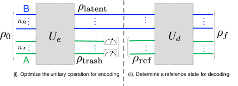
Figure 1: Quantum circuit representation of a quantum autoencoder using a mixed reference state. The network includes two parts: (i) The encoder $U_{e}$ reorganizes the $(n_{A}+n_{B})$-qubit input state $\rho_{0}$ into two parts, i.e., $n_{B}$-qubit state $\rho_{\rm latent}$ contains the useful information (blue lines) that represent the latent qubits and $n_{A}$-qubit state $\rho_{\rm{trash}}$ contains the superfluous information (green lines) that represent the trash qubits. Here, the trash state is obtained by tracing out the latent space of $n_{B}$ qubits. The latent state is obtained by tracing out the trash space of $n_{A}$ qubits. (ii) The decoder $U_{d}$ reconstructs the state $\rho_{f}$ by using the combination of the latent state and ancillary fresh qubits (initialized to the reference state). The goal of the quantum autoencoder is to maximize the overlap between the reconstructed state $\rho_{f}$ and the original state $\rho_{0}$. Note that, we use the common practice of taking the decoding as the inverse of the encoding of $U_{d}=U_{e}^{\dagger}$ pepper2019experimental ; ma2023compression .

In most existing QAE schemes romero2017quantum ; pepper2019experimental ; huang2020realization ; ma2023compression , pure states are utilized as reference states (see $\rho_{\rm{ref}}$ in Fig. 1) for recovering the input state (see $\rho_{0}$ in Fig. 1). There exists an upper bound (hereafter, we call it QAE-pure bound, abbreviated as $Q_{\rm pure}^{\rm bound}$) for the encoding fidelity, i.e., the overlap between the trash state (see $\rho_{\rm{trash}}$ in Fig. 1) and the reference state $\rho_{\rm{ref}}$. According to the results in ma2023compression , an optimal encoder (see $U_{e}$ in Fig. 1) fails to disentangle the initial state $\rho_{0}$ that has a rank higher than the dimension of the latent space, namely, $n_{B}$. This originates from the fact that the encoder $U_{e}$ can only decouple the largest $n_{B}$ eigenvalues of $\rho_{0}$, whose sum is less than one ma2023compression ; cao2021noise . When compressing $\rho_{0}$ with high (rank) entropy, the trash state $\rho_{\rm{trash}}$ tends to have high entropy and consequentially have low overlap with a pure reference state (e.g., setting $\rho_{\rm{ref}}=|0\rangle\langle 0|$). In the decoding stage, the low entropy of a pure state may also limit the entropy of the reconstructed state (see $\rho_{f}$ in Fig. 1). To overcome the entropy inconsistency between the input state $\rho_{0}$ and the reconstructed state $\rho_{f}$ cao2021noise , we remove the limitation of a pure reference state and allow the reference state $\rho_{\rm{ref}}$ to be mixed. In this way, the entropy (mixedness) in the reference state $\rho_{\rm{ref}}$ can assist the decoder to achieve a high fidelity for the reconstructed state $\rho_{f}$.

Most existing QAEs utilize the encoding fidelity between the trash state and the reference state as the cost function to find an optimal encoding map $U_{e}$ romero2017quantum ; pepper2019experimental ; huang2020realization ; ma2023compression . However, this fidelity is different from the decoding fidelity (i.e., the fidelity between the initial state $\rho_{0}$ and the reconstructed state $\rho_{f}$) which characterizes the effectiveness of QAEs in compressing and recovering quantum data. When allowing the reference state to be a mixed state, the encoding fidelity can achieve one by setting $\rho_{\rm{ref}}=\rho_{\rm{trash}}$, whereas the decoding fidelity is usually less than one and can reach one only when perfect disentanglement is realized romero2017quantum . Given that quantum mutual information (QMI) measures the correlation between subsystems of quantum states wilde2011classical ; watrous2018theory , it quantifies the amount of noise that is required to erase (destroy) the correlations completely. To facilitate QAE using mixed reference states, we aim to disentangle the state of $U_{e}\rho_{0}U_{e}^{\dagger}$, which is achieved by minimizing the QMI, i.e., $\mathcal{I}(U_{e}\rho_{0}U_{e}^{\dagger})$ or equivalently maximizing

$$J_{\rm{qmi}}=-\mathcal{I}(U_{e}\rho_{0}U_{e}^{\dagger}),$$ (1)

where $\mathcal{I}(\rho)=S(\textup{Tr}_{A}(\rho))+S(\textup{Tr}_{B}(\rho))-S(\rho)$ denotes QMI of $\rho$ and $S(\rho)=-\textup{Tr}(\rho\ln(\rho))$ denotes the von Neumann entropy of $\rho$. Generally $\mathcal{I}(\rho)\geq 0$, and $\mathcal{I}(\rho)=0$ when $\rho=\textup{Tr}_{A}(\rho)\otimes\textup{Tr}_{B}(\rho)$.

Denote $F(\rho_{1},\rho_{2})$ as the state fidelity between $\rho_{1}$ and $\rho_{2}$ nielsen2010quantum . According to existing research ma2023compression , when training QAEs using the overlap between the trash state and the reference state (e.g., taking the reference state as $\rho_{\rm ref}=|0\rangle\langle 0|$), $J_{\rm{pure}}=F(\textup{Tr}_{B}(U_{e}\rho_{0}U_{e}^{\dagger}),|0\rangle\langle 0|)$ as the cost function, the compression rate of QAEs can approach the theoretical QAE-pure bound. Under that scheme, a high compression rate can be realized for low-rank states ma2023compression . Although this cost function fails to disentangle a high-rank state with satisfactory performance, the optimization of $J_{\rm{pure}}$ leads to a direction of reorganizing the information of initial states into two parts. To combine the cases of low-rank states and high-rank states together, we propose a new cost function,

$$\Phi({\rm{w}})={\rm{w}}J_{\rm{pure}}+(1-{\rm{w}})J_{\rm{qmi}},$$ (2)

where $\rm w\in[0,1]$ controls the ratio of different factors. This protocol is termed QAE-qmi in this paper.

When allowing the reference states to be mixed, we first consider the simple solution of $\rho_{\rm{ref}}=\rho_{\rm{trash}}$ to investigate the effectiveness of training QAEs using $\Phi(\rm w)$. Owing to the physical limitation of preparing arbitrary states, we then investigate mixed reference states with specific constraints. In particular, we consider the case of maximally mixed states blended with pure states. Considering that mixed reference states aim at bringing entropy (mixedness) to the reconstructed states, it is desirable to determine a favorable reference state with good mixedness to recover different states with high efficiency. Each mixed quantum state is physically equivalent to an ensemble of pure states $|\psi_{i}\rangle$ with classical probabilities romero2017quantum ; ma2023compression , i.e., $\rho_{0}=\sum_{i}p_{i}|\psi_{i}\rangle\langle\psi_{i}|$ or an ensemble of mixed states $\rho_{\gamma}$ with classical probabilities, i.e., $\rho_{0}=\sum_{\gamma}p_{\gamma}\rho_{\gamma}$. Similar to standard QAE schemes romero2017quantum ; ma2023compression , the proposed approach can be applied to compress a set of quantum states ($|\psi_{i}\rangle$ or $\rho_{\gamma}$), with a good averaged compression rate regarding classical probabilities ($p_{i}$ or $p_{\gamma}$). In the encoding stage, we may employ the encoding transformation of $U_{e}$ that was optimized for $\rho_{0}$. In the decoding stage, we can use the same reference state $\rho_{\rm{ref}}$ as optimized for $\rho_{0}$ to these individual states ($|\psi_{i}\rangle$ or $\rho_{\gamma}$) to achieve good compression.

To verify the effectiveness of the proposed method, we investigate the experimental implementation of quantum autoencoders with mixed reference states. Since 2016, IBM has made its quantum computers accessible to the general public via remote access, providing a platform for experimentally verifying quantum information tasks ibm2021 . Recently, the compression of tensor products of identical states into smaller dimensions has been implemented on IBM quantum devices pivoluska2022implementation . Inspired by this, we experimentally realize QAE with mixed reference states for compressing general states on the IBM quantum simulator ibmq$\_$qasm$\_$simulator and quantum computer ibmq$\_$quito. This paper is organized as follows. QAE using mixed reference states is firstly elaborated. Then, numerical results on different quantum states are provided. Finally, QAEs are implemented on IBM quantum simulators and quantum computers to compress different quantum states.

II Results

II.1 QAE using mixed reference states

Quantum compression aims at organizing states in a high-dimensional space into two low-dimensional spaces. As illustrated in Fig. 1, we define the trash qubits as subsystem $A$ and the latent qubits as subsystem $B$, respectively. The goal of a quantum autoencoder is to compress $(n_{A}+n_{B})$-qubit state $\rho_{0}$ into $n_{B}$-qubit state $\rho_{\rm latent}$ via an encoder map $U_{e}$ and then recovering to $(n_{A}+n_{B})$-qubit state $\rho_{f}$ via a decoder map $U_{d}$. We denote the dimensions of the original space, the latent space, and the trash space as $d$, $d_{B}$ and $d_{A}$, respectively. After the encoding operation $U_{e}$, the states of the trash space and the latent space are obtained as $\rho_{\rm{trash}}=\textup{Tr}_{B}(U_{e}\rho_{0}U_{e}^{\dagger})$ and $\rho_{\rm latent}=\textup{Tr}_{A}(U_{e}\rho_{0}U_{e}^{\dagger})$, respectively. The efficiency of this task can be quantified by the decoding fidelity between the original state and the reconstructed state, i.e., $J_{d}=F(\rho_{0},\rho_{f})$ and the scheme is considered reliable if $J_{d}$ approaches $1$. During the whole process, a reference state is utilized for two aspects: (i) measure the encoding fidelity between the trash state and the reference state, denoted as $J_{e}=F(\rho_{\rm{trash}},\rho_{\rm{ref}})$; (ii) reproduce the initial states with the combination of the latent state and the reference state. When the unitary $U_{e}$ perfectly disentangles the input state into two parts as $U_{e}\rho_{0}U_{e}^{\dagger}=\rho_{\rm latent}\otimes\rho_{\rm{ref}}$, the overlap between the trash state and the reference state can achieve unity romero2017quantum ; ma2023compression and the decoding fidelity $J_{d}$ can also achieve unity.

In standard QAE, the reference state is usually fixed as a pure state, e.g., $\rho_{\rm ref}=|0\rangle\langle 0|$, and the critical key lies in determining an optimal encoding map $U_{e}$ romero2017quantum . QAE using mixed reference state is complicated in that, apart from searching for the encoding transformation $U_{e}$, additional efforts are required to determine a good mixed reference state $\rho_{\rm{ref}}$ to bring appropriate entropy consistent with the initial states. Whereas, the mechanism of a mixed reference state enables the utilization of the information in the trash state to determine a reference state that can compensate for the entropy inconsistency under fixed $U_{e}$, which potentially increases $J_{d}$ beyond the standard QAE-pure bound. To achieve this, we can take advantage of quantum mutual information (i.e., $J_{\rm{qmi}}$) that measures the disentanglement to guide the optimization of the encoding transformation to narrow the gap between $J_{d}$ and $J_{e}$ (approaching zero when perfect decoupling is reached). The optimization of $J_{\rm{pure}}$ aims to decouple the initial states into two parts, and provides information about the inner structure of initial states, which can be useful for setting the reference state after $U_{e}$ is decided. Instead of searching $U_{e}$ and $\rho_{\rm{ref}}$ together (a full encoding and decoding procedure is required), we accomplish the task of QAEs with mixed reference states within two stages.

The schematic of QAE using a mixed reference state is illustrated in Fig. 1, where the training of QAEs using $\Phi({\rm{w}})={\rm{w}}J_{\rm{pure}}+(1-{\rm w})J_{\rm{qmi}}$ is implemented in the encoding stage, while the mixed reference state is introduced in the decoding stage. After the optimization of $U_{e}$ is finished by maximizing $\Phi$, we determine a reference state for recovery to maximize the overlap between the initial state and the reconstructed state. In particular, we investigate two strategies for setting the reference state: i) taking the trash state as the reference state to make the best use of the information stored in the trash state, ii) taking the mixture of a pure state and a maximally mixed state to allow adaptative mixedness in the reference state.

Recall the nature of QAEs lies in disentangling romero2017quantum . The encoding fidelity that measures the overlap between the trash states and the reference states can reach one (i.e., $J_{e}=1$) by setting $\rho_{\rm{ref}}=\rho_{\rm{trash}}$. Although $J_{d}\leq J_{e}$, in the general case, $J_{d}$ can approach $J_{e}$ and they both achieve one when perfect disentangling is realized ma2023compression . When there is no limitation for the reference state, it is helpful to investigate the performance of QAE-qmi with $\rho_{\rm{ref}}=\rho_{\rm{trash}}$.

In practical applications, it may be useful to utilize reference states with some physical limitations. According to our previous study, a pure reference state, e.g., $|0\rangle\langle 0|$ is effective in compressing low-rank states, with the compression rate approaching the QAE-pure bound ma2023compression , whose value is usually high for low-rank states. For high-rank states with high entropy, the introduction of mixed reference states helps increase the entropy of the reconstructed states cao2021noise . While the maximally mixed states $I/{d_{A}}$ has the highest entropy among all quantum states that belong to $\mathcal{H}_{B}$ and is effective for increasing the entropy in the decoding stage. To achieve a good quantum autoencoder for different quantum states, we take the following reference state

$$\rho_{\rm mix}=p_{r}|0\rangle\langle 0|+(1-p_{r})\frac{I}{d_{A}},$$ (3)

where $p_{r}$ represents the ratio of the pure state and $(1-p_{r})$ represents the ratio of the mixed state in the reference state. $I$ denotes the $d_{A}$-dimensional identity matrix. Different initial states with different inner structures may have different optimal reference states following the form of Eq. (3). When compressing initial states with high entropy, it is preferable to use low $p_{r}$ that generates high entropy for the reference states. As such, it is desirable to specify an optimal $p_{r}$ for different quantum states. $p_{r}$ can be manually set before the training of QAEs based on some prior knowledge or adaptively learned during the training process.

II.2 Thermal states

Given a Hamiltonian $H$, the thermal states corresponding to $H$ have the form of

$$\rho=\frac{e^{-\beta H}}{\textup{Tr}(e^{-\beta H})},$$ (4)

where $\beta$ is the inverse temperature kliesch2019properties . In particular, we consider the Hamiltonian of the one-dimensional transverse-field Ising model as

$$H=-(\sum_{j}Z_{j}Z_{j+1}+\sum_{j}X_{j}),$$ (5)

with couplings set to 1.

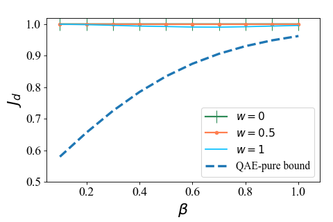
(a) 2-qubit states

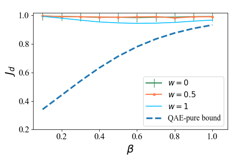
(b) 4-qubit states

Figure 2: Comparison of QAE-qmi under different $\rm w$ using $\rho_{\rm{ref}}=\rho_{\rm{trash}}$. $\beta$ controls the mixedness of the thermal states, i.e., an increase of $\beta$ leads to a decrease of mixedness (entropy) in quantum states. $J_{d}$ represents the decoding fidelity between the initial state and the reconstructed state. $(1-\rm w)$ denotes the ratio of QMI in the cost function $\Phi(\rm w)$. The blue dashed line represents the theoretical upper bound of compression rate when only considering pure reference states ma2023compression .

Firstly, we investigate the performance of different $\rm w$ for the cost function $\Phi({\rm w})={\rm w}J_{\rm{pure}}+(1-{\rm w})J_{\rm{qmi}}$. In particular, we consider three different cases: (i) $\rm w=1$ considers the fidelity between the trash state and a fixed pure state; (ii) $\rm w=0$ considers QMI of the encoding state $U_{e}\rho_{0}U_{e}^{\dagger}$; (iii) $\rm w=0.5$ considers both factors and acts as a more general function. The learning curves in Fig. 2 demonstrate that $\Phi=J_{\rm{qmi}}$ and $\Phi=0.5(J_{\rm{pure}}+J_{\rm{qmi}})$ achieve a similar decoding fidelity, higher than that of $\Phi=J_{\rm{pure}}$. The gaps between $\rm w=0.5$ and $\rm w=1$ suggest that introducing quantum mutual information to the cost function $\Phi(\rm w)$ helps enhance the decoding fidelity for 4-qubit states. The training curves of QAE-qmi under different $\rm w$ are summarized in Appendix A.

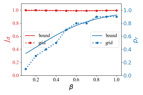
(a) 2-qubit states

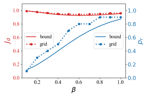
(b) 4-qubit states

Figure 3: Comparison of two strategies of setting $p_{r}$ for compressing and recovering thermal states. $p_{r}$ represents the ratio of the pure state and $(1-p_{r})$ represents the ratio of the mixed state in the reference state. $J_{d}$ represents the fidelity between the initial state and the reconstructed state. The solid blue line (dashed blue line) corresponds to the actual value of $p_{r}$. The solid red line (dashed red line) represents the value of $J_{d}$ through the bound information (grid searching from a set of values).

Then we turn to the case of setting reference states as Eq. (3). It is worth noting that the training of QAEs using $\Phi({\rm w})={\rm w}J_{\rm{pure}}+(1-{\rm w})J_{\rm{qmi}},{\rm w}\in[0,1]$ is iteratively performed in the first stage, while the mixed reference states are determined at the second decoding stage. After the training of $\Phi(\rm w)$ is finished, we introduce a candidate set with different values of $p_{r}$. We implement an example of QAE-qmi using $\rho_{\rm{ref}}=\rho_{\rm mix}$ under different values of $p_{r}$, with detailed information in Appendix C. The comparison between $\Phi=J_{\rm{qmi}}$ and $\Phi=0.5(J_{\rm{pure}}+J_{\rm{qmi}})$ suggests that when limiting the reference state to be the form of (3), $\Phi=J_{\rm{qmi}}$ may have some disadvantages, while $\Phi=0.5(J_{\rm{pure}}+J_{\rm{qmi}})$ achieves good results with appropriate $p_{r}$. As such, we consider $\Phi=0.5(J_{\rm{pure}}+J_{\rm{qmi}})$ to be useful for both $\rho_{\rm{ref}}=\rho_{\rm{trash}}$ and $\rho_{\rm{ref}}=\rho_{\rm mix}$. Hereafter, without specific notation, QAE-qmi refers to the case of $\Phi=0.5(J_{\rm{pure}}+J_{\rm{qmi}})$.

Now, we focus on determining a good $p_{r}$ to reconstruct quantum states with high decoding fidelity. Recall the value of $p_{r}$ determines the mixedness of reference state in the form of Eq. (3), it is natural that quantum states with different inner structures (entropy) may have different optimal $p_{r}$ to achieve an optimal decoding fidelity. Under the fixed cost function $\Phi=0.5(J_{\rm{pure}}+J_{\rm{qmi}})$, we define a candidate set $\{0,0.1,0.2,0.3,0.4,0.5,0.6,0.7,0.8,0.9,1.0\}$ for $p_{r}$ and record the best $p_{r}$ that achieves the highest decoding fidelity for each case. In particular, the optimal $p_{r}$ by means of grid-search is defined as $p_{r}^{\rm grid}$.

It is intuitive that high-rank states with high entropy and low QAE-pure bounds require more mixedness for recovery, i.e., a low $p_{r}$. We assume $p_{r}^{\rm grid}$ might have a relationship with the QAE-pure bound, which reflects the inner structure of the initial states. The value of optimal $p_{r}^{\rm grid}$ tends to approach the square of the QAE-pure bound, which is defined as $p_{r}^{\rm bound}$. We explore two strategies of setting $p_{r}$, i.e., directly drawing inspirations from the QAE-pure bound or grid searching from a set of values. To compare the two strategies, the actual value of $p_{r}$ and the associated decoding fidelity $J_{d}$ for two strategies are summarized in Fig. 3. Clearly, $p_{r}^{\rm grid}$ has the same trend as $p_{r}^{\rm bound}$, and their decoding fidelities are close to each other under different parameters. Please refer to Appendix B for additional results about two ways of setting $p_{r}$.

Based on the observation that the best $p_{r}$ from a grid search strategy is close to the square of QAE-pure bound, we provide two strategies for setting $p_{r}$ in $\rho_{\rm mix}$. (i) For each state $\rho_{0}$, there exists an upper bound which is the sum of partial eigenvalues ma2023compression . Based on the prior knowledge about the initial state to be compressed, we can set empirical values for $p_{r}^{\rm bound}=[Q_{\rm pure}^{\rm bound}(\rho_{0})]^{2}$ to achieve high decoding fidelity. (ii) When prior knowledge about the initial state $\rho_{0}$ is not available, we can infer its inner pattern from the training process. Recall $J_{\rm{pure}}$ is approaching the QAE-pure bound during the training ma2023compression . We can take $p_{r}^{\rm guess}=J_{\rm{pure}}^{2}$ to adaptively set the reference states during the learning process. The comparison results of different strategies of setting $p_{r}$ are summarized in Appendix B, demonstrating that the manual and automatic ways of setting $p_{r}$ are effective in compressing and recovering different quantum states.

II.3 Werner states

A Werner state is a bipartite state that is invariant under any unitary operator of the form of $U\otimes U$ lyons2012werner . Let $|k\rangle$ and $|j\rangle$ be the computational basis for two bipartite subspaces, respectively. A Werner state can be parameterized by

$$\rho(\alpha)=\frac{1}{d^{2}-d\alpha}(I-\alpha\sum_{kj}|kj\rangle\langle jk|),$$ (6)

where $I$ denotes the $d^{2}$-dimensional identity matrix and $\alpha$ varies between -1 and 1. We consider compressing 2-qubit states into 1-qubit states and 4-qubit states into 2-qubit states.

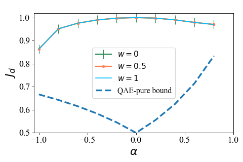
(a) 2-qubit states

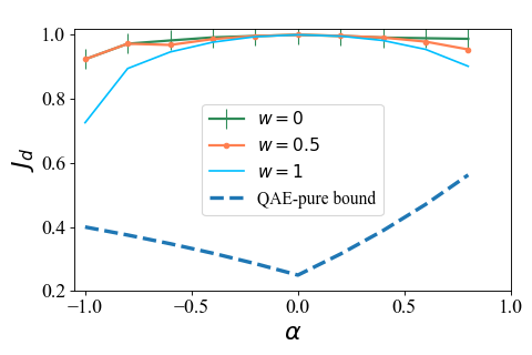
(b) 4-qubit states

Figure 4: Comparison of QAE-qmi under different $\rm w$ for Werner states under $\rho_{\rm{ref}}=\rho_{\rm{trash}}$. $(1-\rm w)$ denotes the ratio of QMI in the new cost function $\Phi(\rm w)$. $J_{d}$ denotes the fidelity between the initial state and the reconstructed state. The blue dashed line represents the theoretical upper bound of compression rate when only considering pure reference states ma2023compression .

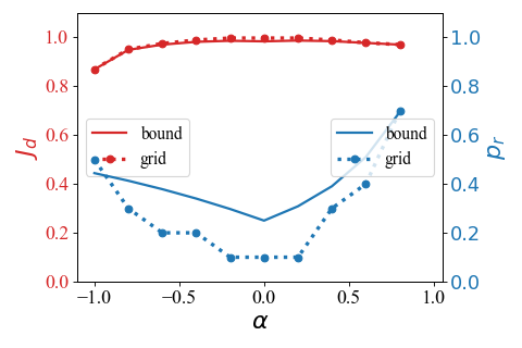
(a) 2-qubit states

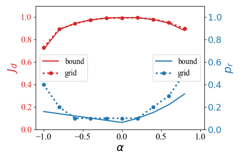
(b) 4-qubit states

Figure 5: Comparison results of two strategies of setting $p_{r}$ when compressing and recovering Werner states. $J_{d}$ represents the fidelity between the initial and reconstructed states. $p_{r}$ represents the ratio of the pure state and $(1-p_{r})$ represents the ratio of the mixed state in the reference state. The solid blue line (dashed blue line) corresponds to the actual value of $p_{r}$. The solid red line (dashed red line) represents the value of $J_{d}$ through the bound information (grid searching from a set of values).

We first investigate the performance of $\rho_{\rm{ref}}=\rho_{\rm{trash}}$, with results of different $\rm w$ summarized in Fig. 4. Likewise, QAE-qmi with $\rm w=0$ and $\rm w=0.5$ achieve better performance than $\rm w=1$, suggesting that the introduction of QMI is effective in compressing and recovering quantum states, especially for Werner states with low QAE-pure bounds (i.e., $\alpha$ approaching -1 or 1). Then we take reference states as the maximally mixed states blended with pure states, i.e., $\rho_{\rm{ref}}=\rho_{\rm mix}$. The actual value of $p_{r}$ from the two strategies and the associated decoding fidelity $J_{d}$ are summarized in Fig. 5. $p_{r}^{\rm grid}$ has the same trend as $p_{r}^{\rm bound}$, and the decoding fidelities of using $p_{r}^{\rm grid}$ and $p_{r}^{\rm bound}$ exhibit similar performance under different parameters. Please refer to Appendix B for numerical results about two strategies of setting $p_{r}$.

II.4 Maximally mixed states blended with pure states

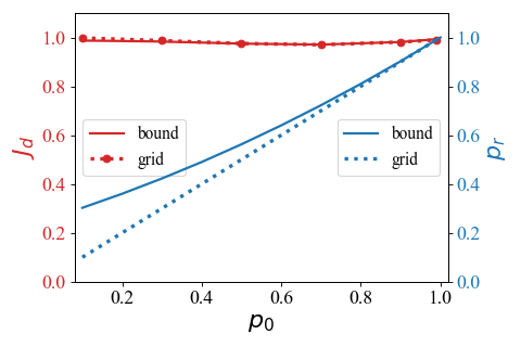
(a) 2-qubit states

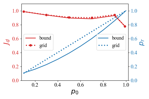
(b) 4-qubit states

Figure 6: Comparison of two strategies of setting $p_{r}$ for compressing maximally mixed states blended with pure states. $p_{r}$ represents the ratio of the pure state and $(1-p_{r})$ represents the ratio of the mixed state in the reference state. $J_{d}$ represents the fidelity between the initial state and the reconstructed state. The solid blue line (dashed blue line) corresponds to the actual value of $p_{r}$. The solid red line (dashed red line) represents the value of $J_{d}$ through the bound information (grid searching from a set of values).

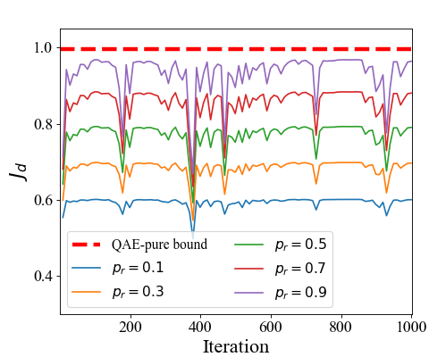
(a) $\rm w=0.5$

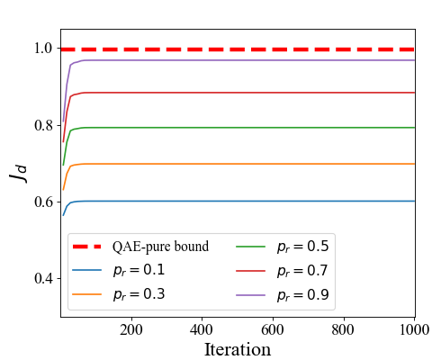
(b) $\rm w=0.99$

Figure 7: An example of QAE-qmi with limited reference states for compressing 2-qubit states with $p_{0}=0.99$. $p_{r}$ represents the ratio of the pure state and $(1-p_{r})$ represents the ratio of the mixed state in the reference state. $J_{d}$ represents the fidelity between the initial state and the reconstructed state. The red dashed line represents the theoretical upper bound of compression rate when only considering pure reference states ma2023compression . (a) training using $J=0.5(J_{\rm{pure}}+J_{\rm{qmi}})$, (b) training using $J=0.99J_{\rm{pure}}+0.01J_{\rm{qmi}}$.

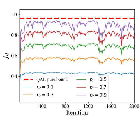
(a) $\rm w=0.5$

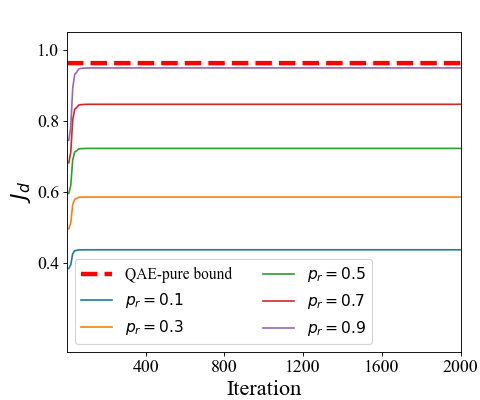
(b) $\rm w=0.99$

Figure 8: An example of QAE-qmi with limited reference states for compressing 4-qubit states with $p_{0}=0.95$. $p_{r}$ represents the ratio of the pure state and $(1-p_{r})$ represents the ratio of the mixed state in the reference state. $J_{d}$ represents the fidelity between the initial state and the reconstructed state. The red dashed line represents the theoretical upper bound of compression rate when only considering pure reference states ma2023compression . (a) training using $J=0.5(J_{\rm{pure}}+J_{\rm{qmi}})$, (b) training using $J=0.99J_{\rm{pure}}+0.01J_{\rm{qmi}}$.

In this subsection, we focus on the initial states that have a similar form to $\rho_{\rm mix}$ as

$$\rho(p_{0})=p_{0}|\psi\rangle\langle\psi|+(1-p_{0})I/d,$$ (7)

where $I$ denotes the $d$-dimensional identity matrix and the value of $p_{0}$ controls the purity of the initial states. By simple computation, we find that states with high $p_{0}$ have a high QAE-pure bound. When taking the reference states as $\rho_{\rm{ref}}=\rho_{\rm mix}$, we observe that the best $p_{r}$ found by means of grid search (i.e., $p_{r}^{\rm grid}$) tends to be the value of $p_{0}$. Recall $p_{r}^{\rm grid}$ is close to the square of the QAE-pure bound for thermal states and Werner states. We compare two strategies of setting $p_{r}$, including $p_{r}^{\rm grid}=p_{0}$ and $p_{r}^{\rm bound}=[Q_{\rm pure}^{\rm bound}(\rho_{0})]^{2}$, with their values and associated decoding fidelities in the same figure with two scales. Judging from Fig. 6, the two curves are close to each other with increasing $p_{0}$. The decoding fidelities for the two strategies of setting $p_{r}$ achieve similar values.

Under the strategy of $p_{r}=p_{r}^{\rm guess}$, we further compare the performance of QAE-qmi under different $\rm w$, with results shown in Appendix C. The drop of decoding fidelity when $p_{0}$ approaches one reveals that $\Phi=0.5(J_{\rm{pure}}+J_{\rm{qmi}})$ hinders the compression of quantum states with high $p_{0}$. To better display this, we provide the training performance of QAE-qmi with $\rm w=0.5$ and $\rm w=0.99$ in Fig. 7 for 2-qubit states and Fig. 8 for 4-qubit states. For states with high purities, training with $\Phi=0.5(J_{\rm{pure}}+J_{\rm{qmi}})$ might lead to fluctuation of decoding fidelity, which can be avoided by reducing the ratio of $J_{\rm{qmi}}$.

II.5 Experimental implementations on quantum devices

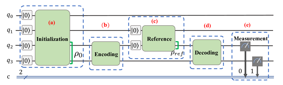
Figure 9: Quantum circuits for compressing 2-qubit states into 1-qubit states and recovering to 2-qubit states using mixed reference states. Firstly, four qubits are required to generate a 4-qubit pure state in (a), whose partial trace on $q_{0}q_{1}$ leads to a mixed state $\rho_{0}$ on $q_{2}q_{3}$. Hereafter, the encoding operation and the decoding operation are performed on $q_{2}q_{3}$, where $q_{2}$ contains the trash state $\rho_{\rm{trash}}$ and $q_{3}$ contains the latent state $\rho_{\rm latent}$. Then, $q_{1}q_{2}$ are reused to generate a pure state whose partial trace on $q_{1}$ leads to a reference state $\rho_{\rm{ref}}$ on $q_{2}$ in (c). Then, the decoding operation in (d) is performed on the combination of $q_{2}$ with $\rho_{\rm{ref}}$ and $q_{3}$ with $\rho_{\rm latent}$. Finally, measurements are performed on $q_{2}q_{3}$ to obtain the reconstructed states in (e).

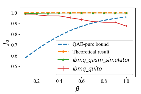
(a) thermal states

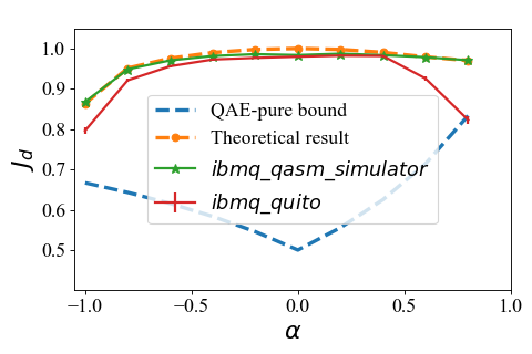
(b) Werner states

Figure 10: Results for quantum autoencoders on ibmq$\_$qasm$\_$simulator and ibmq$\_$quito for encoding and decoding 2-qubit states. $J_{d}$ represents the fidelity between the initial state and the reconstructed state. The blue dashed line represents the upper bound of compression rate when only considering pure reference states ma2023compression . The orange line represents the theoretical results of simulating QAE on classical computers. The green line represents the numerical results obtained from the IBM simulator ibmq$\_$qasm$\_$simulator. The red line represents the average results of 6 times when quantum circuits are sampled with 8192 shots on IBM Quantum device ibmq$\_$quito.

Generally, it is assumed that quantum circuits deal with pure states. We need to find a solution to generate mixed states, which is essential in preparing initial states for compressing and preparing mixed reference states for decoding. We use the technique of purification nielsen2010quantum to associate a mixed state with a pure state in a large space. Given a state $\rho_{K}$ of a quantum system $K$, it is possible to introduce another system $R$, and define a pure state $|\psi\rangle_{KR}$ for the joint system $KR$ such that $\rho_{K}=\textup{Tr}_{R}(|\psi\rangle\langle\psi|_{KR})$. The pure state $|\psi\rangle_{KR}$ reduces to $\rho_{K}$ when we look at the system $K$ alone. This mathematical procedure can be done for any state. Please refer to Appendix E for detailed information about the construction of $|\psi\rangle_{KR}$ for arbitrary $\rho_{K}$.

The quantum circuit for compressing 2-qubit states into 1-qubit states is depicted in Fig. 9, where four qubits $q_{0}q_{1}q_{2}q_{3}$ are utilized to generate mixed states on $q_{2}q_{3}$, on which the encoding gate and the decoding gate are performed. The circuit can be divided into five parts: (a) prepare the initial state for compression, (b) perform the encoding operation, (c) prepare the reference state for decoding, (d) perform the decoding operation, (e) perform quantum measurements to obtain the density matrix of the reconstructed state. In fact, a set of complete measurements are required to specify the density matrix of a quantum state dong2022quantum . In Fig. 9, only a special case of local measurement of $\sigma_{z}\otimes\sigma_{z}$ on $q_{2}q_{3}$ is performed. Adding some gates (such as the Hadamard gate and the $S^{\dagger}$ gate) before the measurement part (i.e., between (d) and (e)) helps realize other measurements. Hence, the quantum circuits are repeated several times until a complete measurement is accomplished. Feeding the measured data to the built-in function for quantum state tomography in qiskit, the density matrix of the reconstructed state is finally obtained.

In this work, we do not perform the optimization loops on quantum devices. Instead, we take the encoding transformation $U_{e}$ and the reference state in the form of Eq. (3) that are learned numerically on classical computers, and then deploy them on IBM quantum simulators and quantum computers, respectively. Note that, each green block in Fig. 9 represents quantum circuits composed of a sequence of quantum gates to achieve unitary operations. Please refer to Appendix E for the transpiled circuits for the green blocks.

We implement the procedure of compressing and recovering 2-qubit states on ibmq$\_$qasm$\_$simulator and ibmq$\_$quito, with $8192$ shots. Each compression task is run 6 times on ibmq$\_$quito. The comparison results are summarized in Fig. 10. The results of the simulators are in agreement with the theoretical results obtained from classical computers. However, gaps exist between the results of ibmq$\_$qasm$\_$simulator and ibmq$\_$quito. In particular, the gap becomes apparent for thermal states with increasing $\beta$ and Werner states with $\alpha$ approaching -1 or 1. The reason might be that compressing those states is sensitive to the noise in $U_{e}$, and thus exhibits inferior performance on ibmq$\_$quito which suffers from a variety of noise sources (e.g., CNOT noise, read-out noise). In particular, we visualize the density matrices of the initial states and the reconstructed states obtained from ibmq$\_$quito for Werner states in Appendix E.

III Discussion

In this paper, we have investigated the performance of QAE with mixed reference states when training using a general cost function. From the numerical comparison of different quantum states, we summarize the characteristics of the protocol as follows.

(i) The proposed function of $\Phi({\rm w})={\rm w}J_{\rm{pure}}+(1-{\rm w})J_{\rm{qmi}}$ combines the approximate QAE-pure bound function that reflects the inner structure of the initial states and the quantum mutual information that measures the correlation between subsystems. It is a general function that can be applied to both low-rank states and high-rank states. As demonstrated by the numerical results, training QAEs using $\Phi(\rm w)$ achieves high decoding fidelity under different reference setting rules including $\rho_{\rm{ref}}=\rho_{\rm{trash}}$ and $\rho_{\rm{ref}}=\rho_{\rm mix}$. In addition, it has been found that for mixed states with high QAE-pure bounds (e.g., large $p_{0}$ in Eq. (7)), it is preferable to increase $\rm{w}$ in $\Phi({\rm w})={\rm w}J_{\rm{pure}}+(1-{\rm w})J_{\rm{qmi}}$, giving more importance to the approximate QAE-pure bound. This is consistent with the fact that pure reference states together with $J_{\rm{pure}}$ are able to realize a good compression rate for low-rank states ma2023compression .

(ii) The numerical results demonstrate that setting the reference state in the form of Eq. (3) helps enhance the decoding fidelity for high-rank states. Due to the special form of the reference states, it is intuitive that different initial states may have different optimal purity ratios $p_{r}$ that help maintain the entropy consistency between the initial states and the reconstructed states. As demonstrated by the numerical results in Fig. 3 and Fig. 5, and Fig. 6, the optimal $p_{r}$ by means of grid search is close to the square of QAE-pure bound for thermal states, Werner states and maximally mixed states blended with pure states. Such findings provide hints for adaptively setting reference states for different quantum states.

(iii) When limiting the reference states to the form of Eq. (3), we can take advantage of the prior information of the states to be compressed to determine a mixed reference state that achieves a high decoding fidelity between the initial state and the reconstructed state. For example, $p_{r}^{\rm bound}=[Q_{\rm pure}^{\rm bound}(\rho_{0})]^{2}$ can be determined before the training process of QAEs. If no prior knowledge is available, we can also obtain a guess of the QAE-pure bound by inferring from the training process and taking $p_{r}^{\rm guess}=J_{\rm{pure}}^{2}$. From this perspective, our QAE-qmi protocol may have wide applications in practical quantum autoencoders.

Our work illustrates the effectiveness of QAEs using mixed reference states under different constraints and thus provides implications for practical applications. More work remains to be investigated in the future. For example, other forms of mixed reference states are worthy of further exploration. Imperfections in quantum system models are not considered in this work. Our future work will also include general quantum channels to deal with decoherence for mixed quantum states.

IV Methods

IV.1 Quantum model

Here, we use the density matrix $\rho(t)$ (which is a Hermitian, positive semidefinite matrix satisfying $\textup{Tr}(\rho(t))=1$ to describe the state of a closed quantum system. The evolution equation for $\rho(t)$ can be described by the quantum Liouville equation dong2010quantum

$${\rm{i}}\dot{\rho}(t)=\rho(t)H(t)-H(t)\rho(t).$$ (8)

When we use control fields $\{u_{j}(t)\}_{j=1}^{M}$ to control the system, the system Hamiltonian in Eq. (8) can be divided into two parts, i.e., $H(t)=H_{0}+H_{c}(t)=H_{0}+\sum_{j=1}^{M}u_{j}(t)H_{j},$ where $H_{0}$ is the time-independent free Hamiltonian of the system, $H_{c}(t)$ is the control Hamiltonian representing the interaction of the system with the control fields. For such a control system, its solution is given as $\rho(t)=U(t)\rho_{0}U^{\dagger}(t)$ with $U(0)=I$, where the propagator $U(t)$ is formulated as follows:

$$\frac{d}{dt}U(t)=-{\rm{i}}[H_{0}+\sum_{j=1}^{M}u_{j}(t)H_{j}]U(t).$$ (9)

For the compression task, we consider spin chain models with

$$H_{0}=\sum_{i=0}^{(n_{A}+n_{B}-1)}(\sigma_{i}^{x}\sigma_{i+1}^{x}+\sigma_{i}^{y}\sigma_{i+1}^{y}+\sigma_{i}^{z}\sigma_{i+1}^{z}).$$

Chains with Heisenberg coupling are known to be controllable given at least two noncommuting controls acting on the first or the last spin in the chain burgarth2009local ; wang2016subspace , we exert control fields on the first two qubits towards $X$ and $Y$ directions dong2023learning , with the control Hamiltonian as $H_{c}=\sum_{k=0,1}(u_{k}^{x}\sigma_{k}^{x}+u_{k}^{y}\sigma_{k}^{y})$. As such, there are four control fields to be designed. We use piece-wise control fields, which means that the total control time $T$ is equally divided into different periods, with each having $dt=T/N$ duration times. In this work, the total control time $T=20$ is equally divided into 100 pieces. The bound of control fields is set as $[-10,10]$. Then, the encoding map for QAEs can be obtained by $U_{e}=U(T)$ following Eq. (9).

IV.2 Training autoencoders using learning algorithms

In this work, the training of a quantum autoencoder is reduced to searching for an optimal $U_{e}$ that maximizes $\Phi({\rm w})={\rm w}J_{\rm{pure}}+(1-{\rm w})J_{\rm{qmi}},{\rm w}\in[0,1]$. After the training is completed, injecting a mixed state $\rho_{\rm{ref}}$ to the decoder helps maintain the entropy consistency between the initial states and the reconstructed states. The reconstructed state is formulated as $\rho_{f}=U_{e}^{\dagger}(\rho_{\rm latent}\otimes\rho_{\rm ref})U_{e}$. Finally, the overlap between the reconstructed states and the original states is measured to evaluate the efficiency of the quantum autoencoder. The procedure of QAE-qmi using mixed reference states is as follows:

1. Randomly initialize $\theta$, where $\theta$ represents the control fields for the systems

2. Apply $U_{e}(\theta)$ to the initial states $\rho_{0}$

3. Measure $\rho_{\rm{trash}}$ and $\rho_{\rm latent}$ and compute function
   $\Phi({\rm w})={\rm w}F(\rho_{\rm{trash}},|0\rangle\langle 0|)-(1-{\rm w})\mathcal{I}(U_{e}\rho_{0}U_{e}^{\dagger})$

4. Perform the optimization of $\Phi(\rm w)$ using learning algorithms and obtain a new control parameter $\theta$

5. Repeat steps 2-4 until convergence

6. Report the classical information $\theta$ and store the latent state $\rho_{\rm latent}$

7. Determine a suitable reference state $\rho_{\rm{ref}}$ using different strategies (e.g., $\rho_{\rm{ref}}=\rho_{\rm{trash}}$ or $\rho_{\rm{ref}}=\rho_{\rm mix}$) and prepare the reference state

8. Perform $U_{e}^{\dagger}(\theta)$ on the combined state $\rho_{\rm latent}\otimes\rho_{\rm{ref}}$ and obtain the reconstructed state as $\rho_{f}$

The key is to optimize the cost function of $\Phi$ using learning algorithms. Evolutionary strategy (ES) methods exhibit an advantage in exploring unknown environments in games salimans2017evolution and have been applied in optimizing quantum control issues shir2009niching . The comparison results in our previous work suggest that ES has the potential to optimize the compression rate towards the theoretical upper bounds with high efficiency ma2023compression . In this work, we utilize ES to optimize the cost function $\Phi(\rm w)$.

ES is a black-box optimization method that utilizes heuristic search procedures inspired by natural evolution. At every iteration (“generation”), a population of parameter vectors (“genotypes”) is perturbed (“mutated”) and their objective function value (“fitness”) is evaluated. The highest-scoring parameter vectors are then recombined to form the population for the next generation, and this procedure is iterated until convergence salimans2017evolution . The detailed description for the ES method is provided in Appendix D.

It is worthy to note that, the initialization process in Step 1 can be formulated as $\theta=\textbf{u}_{\textup{min}}+\textup{Rand}[0,1](\textbf{u}_{\textup{max}}-\textbf{u}_{\textup{min}})$, where $\textup{Rand}[0,1]$ is function generating random numbers uniformly distributed between 0 and 1 to meet the physical restriction of control fields. In addition, boundary checks and resetting values are required for every step that involves new parameters to guarantee that newly generated parameters lie in the constrained field. For the parameter setting of the ES method (see Appendix D), we set the population size as $NP=40$ for 2-qubit states and $NP=50$ for 4-qubit states. The perturbation factor is set as $\delta=0.01$. The learning parameter is set as $\chi_{1}=0.5$. The momentum factor is set as $\chi_{2}=0.9$. The perturbation factor is decayed as $\delta\leftarrow 0.98\delta$ every 100 training iterations.

V ACKNOWLEDGMENTS

This work was supported by the Australian Research Council’s Future Fellowship funding scheme under Project FT220100656, and the Australian Research Council’s Discovery Projects funding scheme DP210101938, and U.S. Office of Naval Research Global under Grant N62909-19-1-2129, and the University of Melbourne through the establishment of the IBM Quantum Network Hub at the University.

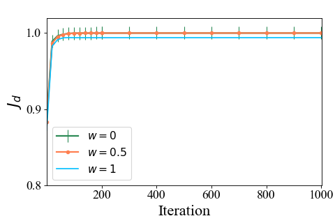
(a1) 2-qubit thermal states

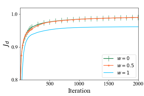
(a2) 4-qubit thermal states

(b1) 2-qubit Werner states

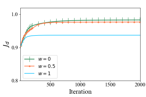
(b2) 4-qubit Werner states

Figure 11: Training process of QAE-qmi using $\rho_{\rm ref}=\rho_{\rm trash}$ under different $\rm w$ for thermal states and Werner states. $(1-\rm w)$ denotes the ratio of QMI in the new cost function $\Phi(\rm w)$. $J_{d}$ denotes the decoding fidelity between the initial and reconstructed states.

Appendix A Training performance of $\rho_{\rm ref}=\rho_{\rm trash}$

First, we investigate the performance of different $\rm w$ in the cost function. The results are summarized in Fig. 11, where $\rm w=0$ and $\rm w=0.5$ achieve the similar performance for both 2-qubit states and 4-qubit states. The gaps between $\rm w=0$ and $\rm w=1$ become large for 4-qubit states. The way of $\rho_{\rm ref}=\rho_{\rm trash}$ is in line with maximizing $J_{\rm qmi}$. Hence, we set $\rm w=0$ with $\Phi=J_{\rm qmi}$ to investigate the performance of QAE using mixed reference states and compare it with the noise-assisted QAE method in cao2021noise (termed as QAE-noise in this paper). The average training curves of the two methods are demonstrated in Fig. 12, where they achieve similar decoding fidelities for 2-qubit states in (a1) and (b1). The gaps in (a2) and (b2) reveal that the advantage of QAE-qmi over QAE-noise becomes apparent for 4-qubit states. The decoding fidelities for different parameters are summarized in Fig. 13. The QAE-pure bound of thermal states increases with $\beta$, and QAE-qmi and QAE-noise both beat the QAE-pure bounds under different values of $\beta$.

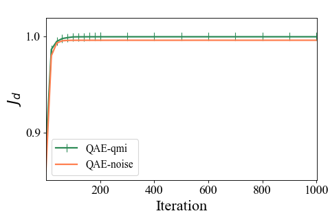
(a1) 2-qubit thermal states

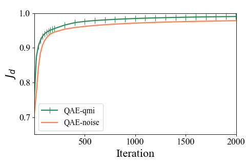
(a2) 4-qubit thermal states

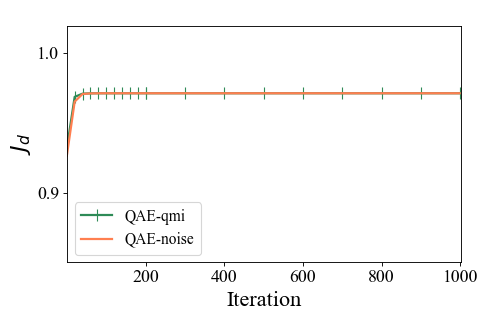
(b1)2-qubit Werner states

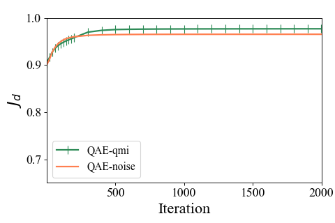
(b2) 4-qubit Werner states

Figure 12: Training process of QAE-qmi vs QAE-noise. QAE-qmi denotes the proposed method that takes $\rho_{\rm ref}=\rho_{\rm trash}$ and $\rm w=0$. QAE-noise denotes the method in cao2021noise . $J_{d}$ denotes the decoding fidelity between the initial state and the reconstructed state.

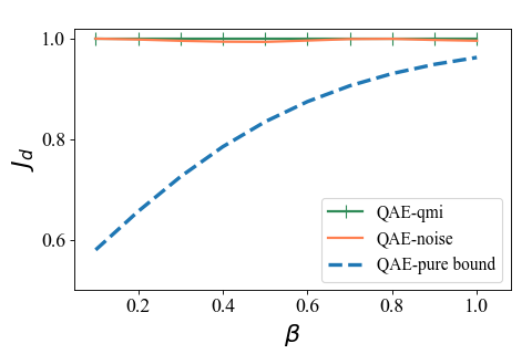
(a1) 2-qubit thermal states

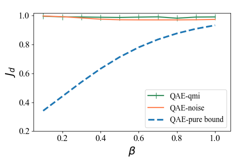
(a2) 4-qubit thermal states

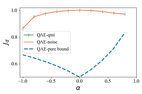
(a1) 2-qubit Werner states

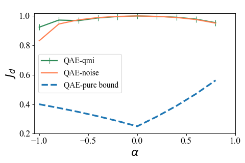
(a2) 4-qubit Werner states

Figure 13: Comparison of QAE-qmi and QAE-noise for compressing different states. $J_{d}$ denotes the decoding fidelity between the initial and reconstructed states. The blue dashed line represents the theoretical upper bound of compression rate when only considering pure reference states ma2023compression .

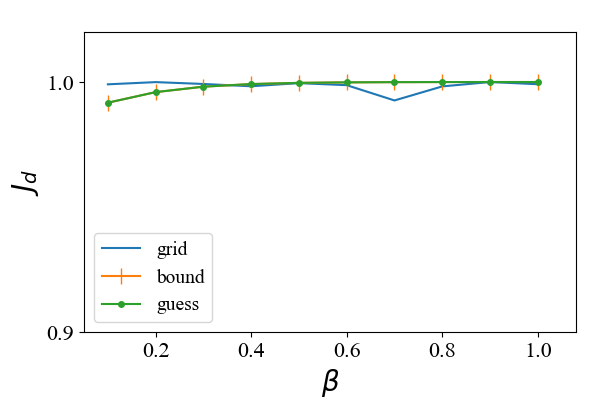
(a1) 2-qubit thermal states

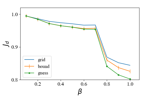
(a2) 4-qubit thermal states

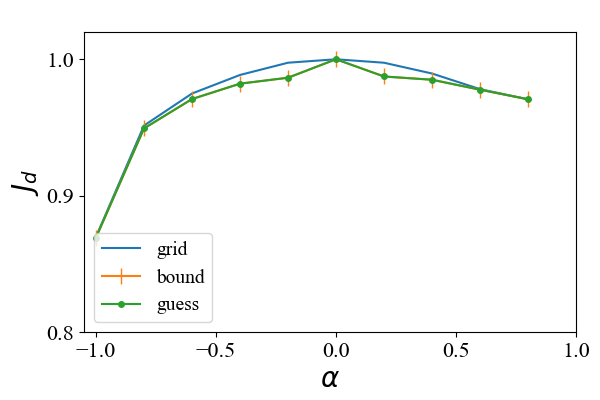
(b1) 2-qubit Werner states

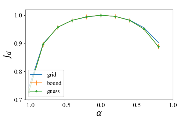
(b2) 4-qubit Werner states

Figure 14: Comparison of different strategies for setting $p_{r}$ when compressing thermal and Werner states. In the legends, grid denotes the strategy of setting $p_{r}$ using grid-search, bound denotes the strategy of setting $p_{r}$ by drawing inspirations from the QAE-pure bound, and guess denotes the way of setting $p_{r}$ by guessing (inferring) from the training process of QAE. $J_{d}$ denotes the decoding fidelity between the initial state and the reconstructed state.

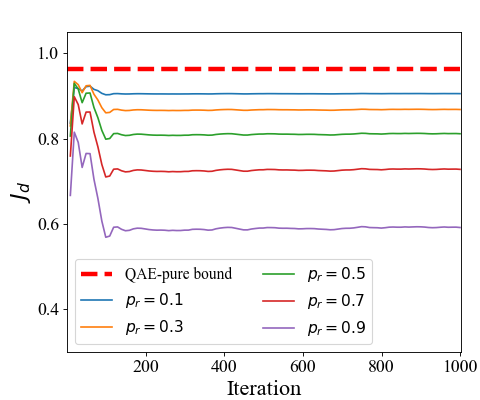
(a) $\rm w=0$

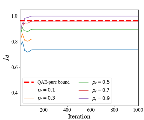
(b) $\rm w=0.5$

Figure 15: An example of QAE-qmi with $\rho_{\rm ref}=\rho_{\rm mix}$ under different $p_{r}$ for 2-qubit thermal states. $p_{r}$ represents the ratio of the pure state in the reference state $\rho_{\rm mix}$ and $(1-p_{r})$ represents the ratio of the mixed state in the reference state $\rho_{\rm mix}$. $J_{d}$ represents the decoding fidelity between the initial and reconstructed states. The red dashed line represents the theoretical upper bound of compression rate when only considering pure reference states ma2023compression .

Appendix B Different strategies for setting $p_{r}$ for $\rho_{\rm ref}=\rho_{\rm mix}$

Numerical results of the three strategies for setting $p_{r}$ for compressing thermal states and Werner states are summarized in Fig. 14. As shown, the curves of $p_{r}^{\rm bound}$ and $p_{r}^{\rm guess}$ exhibit a similar performance, which is also comparable to that of $p_{r}^{\rm grid}$. Those results demonstrate that the manual and automatic strategies of setting $p_{r}$ are effective in compressing and reconstructing different quantum states.

Appendix C Different $\rm w$ under $\rho_{\rm ref}=\rho_{\rm mix}$

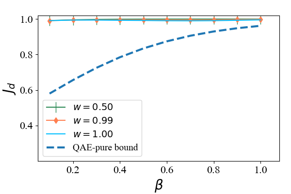
(a1) 2-qubit thermal states

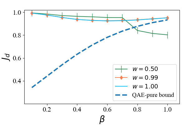
(a2) 4-qubit thermal states

(a) 2-qubit Werner states

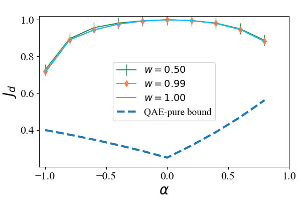
(b) 4-qubit Werner states

Figure 16: Comparison of different ratios in $\Phi(\rm w)$ when compressing thermal and Werner states under $p_{r}=p_{r}^{\rm guess}$. $(1-\rm w)$ denotes the ratio of QMI in the new cost function $\Phi(\rm w)$. The blue dashed line represents the theoretical upper bound of compression rate when only considering pure reference states ma2023compression .

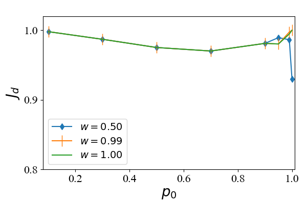
(a) 2-qubit states

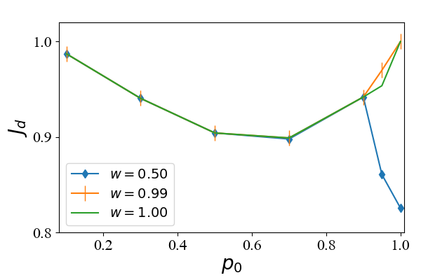
(b) 4-qubit states

Figure 17: Decoding fidelity comparisons between different values of $\rm w$ for compressing maximally mixed states blended with pure states under $p_{r}=p_{r}^{\rm guess}$, where $(1-\rm w)$ denotes the ratio of QMI in the cost function $\Phi(\rm w)$, and $J_{d}$ represents the decoding fidelity between the initial state and the reconstructed state.

In this section, we investigate the performance of $\rm w$ under the reference setting scheme $\rho_{\rm ref}=\rho_{\rm mix}$. We find that when compressing states with high QAE-pure bounds, it is necessary to introduce $J_{\rm pure}$ to allow adaptive mixedness to achieve good decoding fidelities. In particular, we compare the performance of $\Phi=J_{\rm qmi}$ and $\Phi=0.5(J_{\rm pure}+J_{\rm qmi})$ and find that the best $p_{r}$ using grid search tends to lie around zero regardless of the initial states, which means that $I/{d_{A}}$ acts as the reference state. In particular, we provide an example of compressing a thermal state with QAE-pure bound of about 0.95. As shown in Fig. 15, using $\Phi=J_{\rm qmi}$ to train quantum autoencoders, the decoding fidelities for all $p_{r}$ fail to beat the QAE-pure bound. The reason might be that $J_{\rm qmi}$ is in conflict with introducing purity to the reference states (i.e., a high value of $p_{r}$ in $\rho_{\rm mix}$) and merely maximizing $J_{\rm qmi}=S(U_{e}\rho_{0}U_{e}^{\dagger})-S(\rho_{\rm trash})-S(\rho_{\rm latent})$ tends to result in $\rho_{\rm latent}$ with small entropy. Low $p_{r}$ is required to introduce mixedness to the reconstructed state. By comparison, introducing $J_{\rm pure}$ to the cost function as demonstrated in Fig. 15 (b), $p_{r}=0.9$ brings a decoding fidelity closely approaching one, higher than that of $p_{r}=0$ for $\Phi({\rm w})=J_{\rm qmi}$. The introduction of $J_{\rm pure}$ tries to find $U_{e}$ that brings the trash state close to pure states with low entropy, which contributes greatly to the maximization of $J_{\rm qmi}=S(U_{e}\rho_{0}U_{e}^{\dagger})-S(\rho_{\rm trash})-S(\rho_{\rm latent})$. In that case, the latent state may be the mixed one with high entropy. Using $p_{r}=0.9$ for the reference state is enough to achieve a good consistency between the initial state and the reconstructed state.

From Fig. 14, under the reference scheme $\rho_{\rm ref}=\rho_{\rm mix}$, using $\Phi=0.5(J_{\rm pure}+J_{\rm qmi})$ fails to beat QAE-pure bounds for 4-qubit thermal states with large $\beta$ for all the three strategies of setting $p_{r}$. The reason is that 4-qubit thermal states with high $\beta$ have high QAE-pure bounds, and those states can be efficiently compressed using the standard QAE scheme in ma2023compression . This suggests that the introduction of quantum mutual information may hinder the performance of low-rank states. To maintain good results, it is required to decay the ratio of QMI (i.e., to decrease the value of $\rm w$ in the general function $\Phi(\rm{w})$. Hence, we investigate the performance of $\Phi=0.99J_{\rm pure}+0.01J_{\rm qmi}$. The results under the reference scheme $p_{r}=p_{r}^{\rm guess}$ are summarized in Fig. 16. Clearly, 4-qubit states with high $\beta$ are sensitive to the value of $\rm w$, since the performance of $p_{r}=0.5$ is worse than $\rm w=1$ and $\rm w=0.99$. We further compare the performance of QAE-qmi for the mixture of maximally mixed states and the pure states with results summarized in Fig. 17. The drop of decoding fidelity with $p_{0}$ approaching one reveals that $\Phi=0.5(J_{\rm pure}+J_{\rm qmi})$ hinders the decoding fidelity for states with high $p_{0}$. For such states, increasing the ratio of $J_{\rm pure}$ (i.e., increasing the value of $\rm{w}$) is useful.

Appendix D Description of ES

Denote the control fields as a column vector $\theta$ and denote $\Phi(\theta)$ the loss function. Given the population size $NP$, the learning rate $\chi_{1}$, the momentum coefficient $\chi_{2}$, and the permutation factor $\delta$, the procedure of ES is as follows.

1. Randomly initialize the mean vector $\bar{\theta}$

2. Initialize the gradient $d\Phi=0$ and momentum $dv=0$

3. Repeat for each individual $i=1,...,NP$

   1. Sample variation $\epsilon_{i}\sim N(0,I)$

   2. Set mutation variant as $X_{i}\leftarrow\bar{\theta}+\delta\epsilon_{i}$

4. Obtain the gradient $d\Phi\leftarrow\frac{1}{NP\delta}\sum_{i=1}^{NP}\Phi(X_{i})\epsilon_{i}$

5. Obtain the momentum $dv\leftarrow\chi_{2}dv+(1-\chi_{2})d\Phi$

6. Update the new mean vector $\bar{\theta}\leftarrow\bar{\theta}+\chi_{1}dv$

7. If convergent, go to 8; otherwise, go to 3

8. Optimal control parameters $\theta^{*}=\bar{\theta}$

Appendix E Implementation details on quantum states preparation and unitary transformations

Given a state $\rho_{K}$ of a quantum system $K$, it is possible to introduce another system $R$, and define a pure state $|\psi\rangle_{KR}$ for the joint system $KR$ such that $\rho_{K}=\textup{Tr}_{R}(|\psi\rangle\langle\psi|_{KR})$. Suppose $\rho_{K}$ has orthonormal decomposition $\rho_{K}=\sum_{i}p_{i}|i^{K}\rangle\langle i^{K}|$. To purify $\rho_{K}$, a system $R$ with the same state space as system $K$ with orthonormal basis states $|i^{R}\rangle$ is introduced. Then, we can define a pure state for the combined system as $|\psi\rangle_{KR}=\sum_{i}\sqrt{p_{i}}|i^{K}\rangle|i^{R}\rangle.$ Its reduced state for system $K$ reads

$$\textup{Tr}_{R}(|\psi\rangle\langle\psi|_{KR})= \sum_{ij}\sqrt{p_{i}p_{j}}|i^{K}\rangle\langle j^{K}|\textup{Tr}(|i^{R}\rangle\langle j^{R}|)$$

$$= \sum_{ij}\sqrt{p_{i}p_{j}}|i^{K}\rangle\langle j^{K}|\delta_{ij}$$

$$=\rho_{K}.$$

In this work, we set the orthonormal basis states $|i^{R}\rangle$ as the computational basis $|0\rangle,|1\rangle,...$ to generate the associated pure states in the space of $KR$.

When deploying a unitary transformation on quantum devices, we need to obtain the equivalent of quantum gates that realize the desired unitary transformation. In particular, we utilize the embed function Initialization in qiskit to obtain a sequence of quantum gates that can prepare the target states (i.e., (a) and (c) in Fig. 9 in the main text). Also, we utilize the embed function Decomposition in qiskit to obtain a sequence of gates that achieve the target transformation $U_{e}$ and $U_{d}=U_{e}^{\dagger}$ shende2005synthesis (i.e., (b) and (d) in Fig. 9 in the main text).

Here, we provide an example of compressing a 2-qubit Werner state with $\alpha=0$ on ibmq$\_$qasm$\_$simulator in Fig. 18. $U_{e}$ is decomposed into three 2-qubit CNOT gates and eight 1-qubit $U_{3}$ gates, where each $U_{3}$ gate is represented as $U_{3}(\tau,\phi,\lambda)=\left(\begin{array}[]{cc}\cos\left(\frac{\tau}{2}\right)&-e^{\rm{i}\lambda}\sin\left(\frac{\tau}{2}\right)\\ e^{\rm{i}\phi}\sin\left(\frac{\tau}{2}\right)&e^{\rm{i}(\phi+\lambda)}\cos\left(\frac{\tau}{2}\right)\end{array}\right).$

When deploying a sequence of gates on a real quantum computer, some gates can be further decomposed and transpiled into basic gates that are available on the specific quantum device. The transpiled circuits on ibmq$\_$quito for compressing a 2-qubit Werner state with $\alpha=0$ are summarized in Fig. 19, where only four qubits are utilized among the five available qubits.

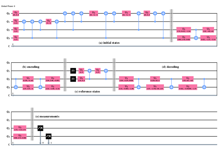
Figure 18: An example of transpiled circuits on ibmq$\_$qasm$\_$simulator for compressing a 2-qubit Werner state with $\alpha=0$. The vertical barriers separate different areas of the proposed method, including (a) prepare the initial state, (b) perform the encoding operation, (c), prepare the reference state, (d) perform the decoding operation, (e) perform measurements.

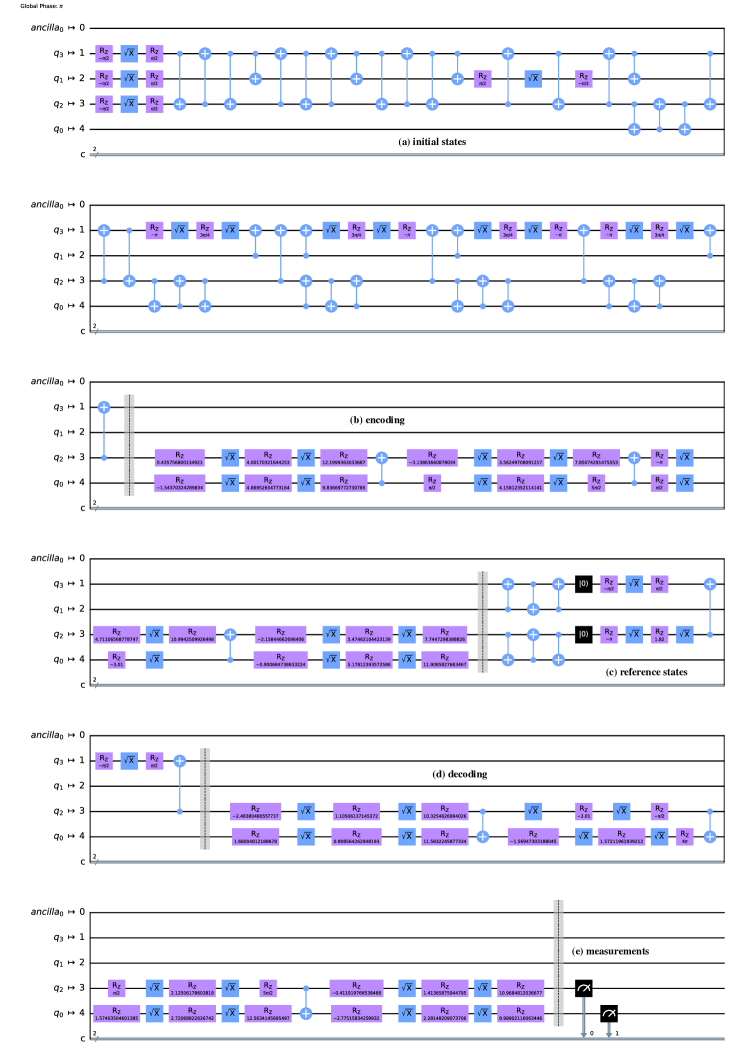
Figure 19: An example of transpiled circuits on ibmq$\_$quito for compressing a 2-qubit Werner state with $\alpha=0$. The vertical barriers separate different stages of the proposed method, including (a) prepare the initial state, (b) perform the encoding operation, (c) prepare the reference state, (d) perform the decoding operation, (e) perform measurements.

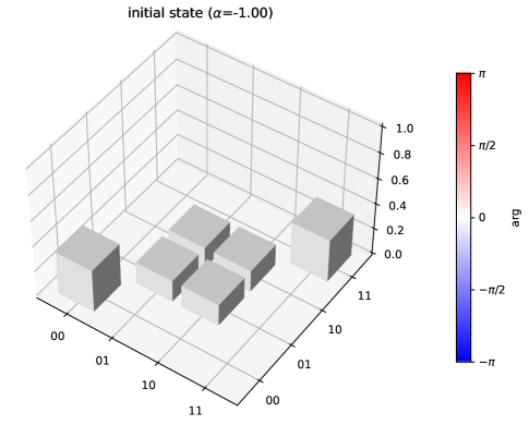
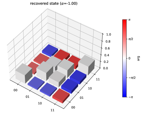
(a) $\alpha=-1$

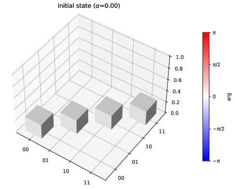
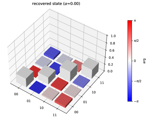
(b) $\alpha=0.0$

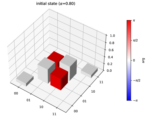
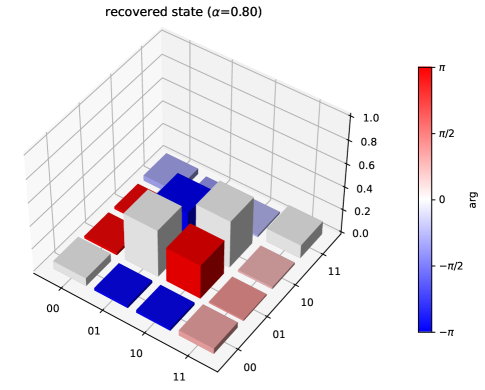
(c) $\alpha=0.8$

Figure 20: Density matrices of the initial states and the reconstructed states obtained from ibmq$\_$quito for 2-qubit Werner states. The provided figure illustrates three instances of compressing Werner states with different parameters: $\alpha=-1.00$, $\alpha=0.00$, and $\alpha=0.80$. Each 2-qubit state is represented by a $4\times 4$ complex matrix, where each element (typically a complex number) is visually depicted as a cylinder. The height of the cylinder represents the amplitude, and the color corresponds to the phase. The density matrices of the reconstructed states (in the second column) closely resemble the density matrices of the initial states (in the first column). This demonstrates an effective compression of 2-qubit Werner states, preserving essential characteristics in the reconstructed states.

References

- (1) Biamonte, J. et al. Quantum machine learning. Nature 549, 195 (2017).
- (2) Dong, D., Chen, C., Li, H. & Tarn, T.-J. Quantum reinforcement learning. IEEE Transactions on Systems, Man, and Cybernetics, Part B (Cybernetics) 38, 1207–1220 (2008).
- (3) Huang, H.-Y. et al. Power of data in quantum machine learning. Nature Communications 12, 1–9 (2021).
- (4) Cerezo, M., Verdon, G., Huang, H.-Y., Cincio, L. & Coles, P. J. Challenges and opportunities in quantum machine learning. Nature Computational Science 2, 567–576 (2022).
- (5) Niu, M. Y., Boixo, S., Smelyanskiy, V. N. & Neven, H. Universal quantum control through deep reinforcement learning. npj Quantum Information 5, 33 (2019).
- (6) Li, J.-A. et al. Quantum reinforcement learning during human decision-making. Nature Human Behaviour 4, 294–307 (2020).
- (7) Dong, D. & Petersen, I. R. Quantum estimation, control and learning: opportunities and challenges. Annual Reviews in Control 54, 243–251 (2022).
- (8) Pu, Y. et al. Variational autoencoder for deep learning of images, labels and captions. In Advances in Neural Information Processing Systems, 2352–2360 (2016).
- (9) Bartůšková, L. et al. Optical implementation of the encoding of two qubits to a single qutrit. Physical Review A 74, 022325 (2006).
- (10) Steinbrecher, G. R., Olson, J. P., Englund, D. & Carolan, J. Quantum optical neural networks. npj Quantum Information 5, 60 (2019).
- (11) Lamata, L., Alvarez-Rodriguez, U., Martín-Guerrero, J. D., Sanz, M. & Solano, E. Quantum autoencoders via quantum adders with genetic algorithms. Quantum Science and Technology 4, 014007 (2018).
- (12) Ding, Y., Lamata, L., Sanz, M., Chen, X. & Solano, E. Experimental implementation of a quantum autoencoder via quantum adders. Advanced Quantum Technologies 2, 1800065 (2019).
- (13) Aspuru-Guzik, A., Dutoi, A. D., Love, P. J. & Head-Gordon, M. Simulated quantum computation of molecular energies. Science 309, 1704–1707 (2005).
- (14) Wan, K. H., Dahlsten, O., Kristjánsson, H., Gardner, R. & Kim, M. Quantum generalisation of feedforward neural networks. npj Quantum Information 3, 36 (2017).
- (15) Romero, J., Olson, J. P. & Aspuru-Guzik, A. Quantum autoencoders for efficient compression of quantum data. Quantum Science and Technology 2, 045001 (2017).
- (16) Bravo-Prieto, C. Quantum autoencoders with enhanced data encoding. Machine Learning: Science and Technology 2, 035028 (2021).
- (17) Pepper, A., Tischler, N. & Pryde, G. J. Experimental realization of a quantum autoencoder: The compression of qutrits via machine learning. Physical Review Letters 122, 060501 (2019).
- (18) Huang, C.-J. et al. Realization of a quantum autoencoder for lossless compression of quantum data. Physical Review A 102, 032412 (2020).
- (19) Bondarenko, D. & Feldmann, P. Quantum autoencoders to denoise quantum data. Physical Review Letters 124, 130502 (2020).
- (20) Achache, T., Horesh, L. & Smolin, J. Denoising quantum states with quantum autoencoders–theory and applications. arXiv preprint arXiv:2012.14714 (2020).
- (21) Zhang, X.-M. et al. Generic detection-based error mitigation using quantum autoencoders. Physical Review A 103, L040403 (2021).
- (22) Du, Y. & Tao, D. On exploring practical potentials of quantum auto-encoder with advantages. arXiv preprint arXiv:2106.15432 (2021).
- (23) Srikumar, M., Hill, C. D. & Hollenberg, L. C. Clustering and enhanced classification using a hybrid quantum autoencoder. Quantum Science and Technology 7, 015020 (2021).
- (24) Zhang, H. et al. Resource-efficient high-dimensional subspace teleportation with a quantum autoencoder. Science Advances 8, eabn9783 (2022).
- (25) Ma, H. et al. On compression rate of quantum autoencoders: Control design, numerical and experimental realization. Automatica 147, 110659 (2023).
- (26) Cao, C. & Wang, X. Noise-assisted quantum autoencoder. Physical Review Applied 15, 054012 (2021).
- (27) Wilde, M. M. From classical to quantum Shannon theory. arXiv preprint arXiv:1106.1445 (2011).
- (28) Watrous, J. The theory of Quantum Information (Cambridge University Press, 2018).
- (29) Nielsen, M. A. & Chuang, I. L. Quantum Computation and Quantum Information (Cambridge University Press, 2010).
- (30) IBM quantum, https://quantum-computing.ibm.com (2021).
- (31) Pivoluska, M. & Plesch, M. Implementation of quantum compression on IBM quantum computers. Scientific Reports 12, 5841 (2022).
- (32) Kliesch, M. & Riera, A. Properties of thermal quantum states: Locality of temperature, decay. Thermodynamics in the Quantum Regime: Fundamental Aspects and New Directions 195, 481 (2019).
- (33) Lyons, D. W., Skelton, A. M. & Walck, S. N. Werner state structure and entanglement classification. Advances in Mathematical Physics 2012 (2012).
- (34) Dong, D. & Petersen, I. R. Quantum control theory and applications: a survey. IET Control Theory & Applications 4, 2651–2671 (2010).
- (35) Burgarth, D., Bose, S., Bruder, C. & Giovannetti, V. Local controllability of quantum networks. Physical Review A 79, 060305 (2009).
- (36) Wang, X., Burgarth, D. & Schirmer, S. Subspace controllability of spin- chains with symmetries. Physical Review A 94, 052319 (2016).
- (37) Dong, D. & Petersen, I. R. Learning and Robust Control in Quantum Technology (Springer Nature, Switzerland AG, 2023).
- (38) Salimans, T., Ho, J., Chen, X., Sidor, S. & Sutskever, I. Evolution strategies as a scalable alternative to reinforcement learning. arXiv preprint arXiv:1703.03864 (2017).
- (39) Shir, O. M. & Bäck, T. Niching with derandomized evolution strategies in artificial and real-world landscapes. Natural Computing 8, 171–196 (2009).
- (40) Shende, V. V., Bullock, S. S. & Markov, I. L. Synthesis of quantum logic circuits. In Proceedings of the 2005 Asia and South Pacific Design Automation Conference, 272–275 (2005).