Evolution of a Water-rich Atmosphere Formed by a Giant Impact on an Earth-sized Planet

Abstract

The atmosphere of a terrestrial planet that is replenished with secondary gases should have accumulated hydrogen-rich gas from its protoplanetary disk. Although a giant impact blows off a large fraction of the primordial atmosphere of a terrestrial planet in the late formation stage, the remaining atmosphere can become water-rich via chemical reactions between hydrogen and vaporized core material. We find that a water-rich post-impact atmosphere forms when a basaltic or CI chondrite core is assumed. In contrast, little post-impact water is generated for an enstatite chondrite core. We investigate the X-ray- and UV-driven mass loss from an Earth-mass planet with an impact-induced multi-component H₂–He–H₂O atmosphere for Gyrs. We show that water is left in the atmosphere of an Earth-mass planet when the low flux of escaping hydrogen cannot drag water upward via collisions. For a water-dominated atmosphere to form, the atmospheric mass fraction of an Earth-mass planet with an oxidizing core after a giant impact must be less than a few times $0.1$%. We also find that Earth-mass planets with water-dominated atmospheres can exist at semimajor axes ranging from a few times 0.1 au to a few au around a Sun-like star depending on the mass loss efficiency. Such planets are important targets for atmospheric characterization in the era of JWST. Our results indicate that efficient mixing between hydrogen and rocky components during giant impacts can play a role in the production of water in an Earth-mass planet.

1 Introduction

Exoplanets as small as Earth are now being discovered by ground-based and spaceborne telescopes. In the proximity of a central star with orbital periods of less than about 100 days, small planets with radii of $\leq$3 $R_{\oplus}$ are more common than Neptune-sized or larger planets. (Petigura et al., 2013; Dressing & Charbonneau, 2015). Statistical studies on the population of small planets from Kepler found that the intriguing transition between bare rocky planets and planets with atmospheres of typically $<$10 wt% (Weiss & Marcy, 2014; Rogers, 2015), known as the radius gap, lies around 1.5–2 $R_{\oplus}$ (Fulton & Petigura, 2018; Hirano et al., 2018). Also, the mass-radius relationships of exoplanets with radii smaller than $1.5\,R_{\oplus}$ suggests that they may have rocky compositions similar to that of Earth (e.g. Zeng et al., 2019).

This study focuses on Earth-sized planets. Earth-sized rocky planets possess only thin or nonexistent atmospheres (Rogers, 2015), although they may have accumulated dense atmospheres in the stage of planet formation. The primordial atmosphere of a terrestrial planet originates from nebular gas rich in H₂/He-rich (Ikoma & Hori, 2012; Lee et al., 2018). A large fraction of the H₂/He atmosphere can be lost by a giant impact event. A head-on collision causes atmospheric blow-off when the velocity of the ground motion resulting from a strong shock exceeds the escape velocity on the planetary surface (Ahrens, 1993; Genda & Abe, 2003; Schlichting et al., 2015). In contrast, oblique impacts that frequently occur in the giant impact stage remove the primordial atmosphere less efficiently (Kegerreis et al., 2020; Denman et al., 2022).

Giant impacts that induce strong turbulence also lead to atmospheric pollution by vaporizing rocky material. In particular, head-on collisions with high impact velocities drive violent mixing between the primordial atmosphere and core material (e.g., Kurosaki & Inutsuka, 2023). The consumption of hydrogen by FeO in the rocky vapor forms a H₂–H₂O atmosphere at a high temperature of $\gtrsim$3000 K. Moreover, if the melt is not metal-saturated after a giant impact, the disk-oriented atmosphere can produce H₂O by reducing a molten mantle during the magma ocean period (Lange & Ahrens, 1982; Matsui & Abe, 1986; Ikoma & Genda, 2006; Lupu et al., 2014; Itcovitz et al., 2022; Lichtenberg et al., 2022; Maurice et al., 2023).

The atmospheric mass and composition of a planet change during the planet’s long-term evolution. After a giant impact, an Earth-sized planet with H₂–H₂O atmosphere would be expected to be exposed to strong X-ray and extreme-UV (XUV) radiation from its host star. An incident XUV flux drives the atmospheric escape from an Earth-sized planet (Zahnle et al., 1988; Hamano et al., 2013). The hydrodynamic escape in the multi-component atmosphere is driven by major species. As a result, the processes of XUV-driven mass loss lead to mass-dependent fractionation in the atmosphere (e.g., Hunten et al., 1987; Johnstone, 2020; Yoshida & Kuramoto, 2021; Yoshida et al., 2022). If the hydrodynamic blow-off of light gases does not carry along heavy gases, the hydrodynamic escape of a planet with a H₂–H₂O atmosphere results in an increase of H₂O in the atmosphere. Note that photochemical reactions via UV photons promote disequilibrium chemistry, such as the production of hydrocarbons, if carbon-bearing molecules such as CH₄ are abundant in the impact-generated atmosphere of an Earth-sized planet.

The phenomenon of energy-limited hydrodynamic escape has been well examined for sub-/super-Earths having H₂/He atmospheres (e.g., Owen & Wu, 2013; Lopez & Fortney, 2014; Hori & Ogihara, 2020) and H₂O-rich atmospheres (e.g., Kurosaki et al., 2014). Recently, Yoshida et al. (2022) calculated the mass loss of the H₂-H₂O atmosphere of an Earth-mass planet near the habitable zone around TRAPPIST-1-like stars coupled with chemical reactions and radiative cooling by H₂O, OH, H${}^{+}_{3}$, and OH⁺. They found that the atmospheric escape rate of H₂ decreases as the initial H₂O/H₂ ratio increases. However, it is not obvious that an Earth-mass planet can retain a water-rich atmosphere over Gyrs after giant impacts. In this study, we calculate the long-term evolution of the water mass fraction in an impact-generated atmosphere of an Earth-mass planet around a Sun-like star under various initial conditions, such as different initial atmospheric masses and semimajor axes. We consider the multi-component hydrodynamic escape of a H₂/He–H₂O atmosphere by photoevaporation under stellar XUV irradiation. We also perform the Smoothed Particle Hydrodynamic (SPH) simulation of giant impacts on an Earth-mass planet with a primordial H₂/He atmosphere and then calculate chemical reactions between the remaining hydrogen and rocky vapor to determine the atmospheric compositions of the planet after giant impacts.

This paper is structured as follows. Section 2 describes our numerical models of mass loss from planetary atmospheres. In Section 3, we show the atmospheric compositions of an Earth-mass planet after giant impacts and the long-term atmospheric evolution through photoevaporation. In Section 4, we calculate the chemical reaction between the rock vapor and the primordial atmosphere and show the SPH simulation results. We also derive analytically the conditions necessary for the water-dominated atmosphere of an Earth-mass planet after the hydrodynamic escape. We summarize our results in the last section.

2 Model description

We examine a one-dimensional, long-term evolution of an Earth-mass planet with the impact-generated atmosphere after giant impacts using the following numerical models. The planetary atmosphere is in radiative-convective equilibrium. (see Kurosaki & Ikoma, 2017, for details).

• The planetary interior is a one-dimensional, fully convective, layered core-envelope structure in hydrostatic equilibrium.

• The planetary atmosphere is in a one-dimensional plain-parallel, radiative-convective equilibrium.

The following subsections summarize our models. Figure 1 shows a schematic of our interior model.

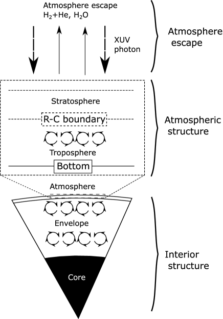
Figure 1: Schematic of our planetary model. The planetary interior is composed of two parts: a spherical symmetry convective interior and a plane-parallel radiative-convective (R-C) equilibrium atmosphere. The interior structure in spherical symmetry is composed of a rocky core and H₂-He-H₂O envelope. The plane-parallel atmosphere is composed of H₂-He-H₂O (see also Section 3.2).

2.1 Interior structure

We consider an Earth-mass planet that initially has a H₂-He atmosphere atop a rocky core. Each layer in the interior is homogeneously mixed and fully convective. We determine the interior structure by solving the following equations,

$$\frac{\partial P}{\partial M_{r}} = -\frac{GM_{r}}{4\pi r^{4}},$$ (1)

$$\frac{\partial r}{\partial M_{r}} = \frac{1}{4\pi r^{2}\rho},$$ (2)

$$\frac{\partial T}{\partial M_{r}} = -\frac{GM_{r}}{4\pi r^{4}}\frac{T}{P}\nabla,$$ (3)

$$\frac{\partial L_{r}}{\partial M_{r}} = -T\frac{\mathrm{d}S}{\mathrm{d}t},$$ (4)

where $r$ is the planetocentric distance, $M_{r}$ is the mass contained in the sphere of radius $r$, $P$ is the pressure, $\rho$ is the density, $T$ is the temperature, $G$ is the gravitational constant, $S$ is the specific entropy, $L_{r}$ is the total energy flux passing through a sphere of radius $r$, and $t$ is time. The symbol $\nabla$ is the adiabatic temperature gradient with respect to pressure, namely,

$$\nabla=\nabla_{\mathrm{ad}}=\left(\frac{\partial\ln T}{\partial\ln P}\right)_{S}.$$ (5)

As for the equations of state (EoS), we use Saumon et al. (1995) for hydrogen and helium and the M-ANEOS (Thompson & Lauson, 1972; Melosh, 2007; Thompson et al., 2019) of basalt for a rocky core (Pierazzo et al., 2005). A giant impact onto an Earth-mass planet causes the dynamic mixing of a H₂-He atmosphere with vaporized core material. Chemical reactions between hydrogen and rocky vapor produce hydrogen-bearing molecules, such as H₂O. We use the M-ANEOS of H₂O, which is one of the dominant components in the atmosphere after a giant impact (see Section 3.2 for details). We adopt the solar composition of the mass fraction of hydrogen $X=0.72$ and helium $Y=0.28$ as the initial envelope composition when the envelope has no rocky vapor (Lodders & Palme, 2009). Integrating equation (4), we obtain the intrinsic luminosity $L_{\mathrm{int}}$ as

$$L_{\mathrm{int}}=-\left[\frac{\mathrm{d}S_{\mathrm{env}}}{\mathrm{d}t}\int_{M_{c}}^{M_{p}}TdM_{r}+\frac{\mathrm{d}S_{\mathrm{c}}}{\mathrm{d}t}\int_{0}^{M_{c}}TdM_{r}\right],$$ (6)

where $S_{\mathrm{env}}$ and $S_{c}$ are the specific entropies of the envelope and the core, respectively, $M_{\mathrm{p}}$ is the total mass of a planet, and $M_{c}$ and $M_{\mathrm{env}}$ are the masses of the core and envelope, respectively. The intrinsic luminosity $L_{\mathrm{int}}$ is also written as $L_{\mathrm{int}}=4\pi R_{p}^{2}F_{\mathrm{top}}$ where $R_{p}$ is the planetary radius and $F_{\mathrm{top}}$ is the outgoing flux from the top of the atmosphere (e.g., Kurosaki & Ikoma, 2017).

2.2 Atmospheric structure

We assume a plane-parallel atmosphere in radiative-convective equilibrium. As shown in Section 3.2, the rock-polluted atmosphere after a giant impact consists mainly of H₂, He, and H₂O. The bottom of the atmosphere is assumed to be at $P_{\mathrm{btm}}$ = 1000 bars. Note that the condensation of molecular species occurs below $P_{\mathrm{btm}}$. The temperature profile in the radiative atmosphere (i.e., the stratosphere) follows the analytical formula derived by Matsui & Abe (1986):

$$\sigma T^{4}=F_{\mathrm{top}}\left(\frac{\tau+1}{2}\right)+\frac{\sigma T_{\mathrm{eq}}^{4}}{2}\left[1+\frac{\kappa_{\mathrm{th}}}{\kappa_{\mathrm{v}}}+\left(\frac{\kappa_{\mathrm{v}}}{\kappa_{\mathrm{th}}}-\frac{\kappa_{\mathrm{th}}}{\kappa_{\mathrm{v}}}\right)e^{-\tau_{\mathrm{v}}}\right],$$ (7)

where $F_{\mathrm{top}}$ is the net flux, $\sigma$ is the Stefan–Boltzmann constant, $T_{\mathrm{eq}}$ is the equilibrium temperature, and $\kappa_{\mathrm{th}}$ (cm${}^{2}\,$g^-1) and $\kappa_{\mathrm{v}}$ (cm${}^{2}\,$g^-1) are the mean opacities for long- and short-wavelength radiation, respectively. The optical depths for long- and short-wavelength radiation are denoted by $\tau$ and $\tau_{\mathrm{v}}$, respectively. The optical depth $\tau$ is defined as $d\tau=-\rho\kappa_{\mathrm{th}}dr$. Here we adopt the Rosseland opacity for $\kappa_{\mathrm{th}}$. The H₂ and He opacities are calculated from the data table given in Freedman et al. (2008). The opacity of H₂O is calculated from line profiles (Rothman et al., 1998) using the HITRAN 2020 database (Gordon et al., 2022). We assume that $\kappa_{\mathrm{v}}=0.1\kappa_{\mathrm{th}}$ (Guillot, 2010). We consider the absorption of the radiation under the assumptions of zero reflectivity and scattering. Then, $\kappa_{\mathrm{th}}$ in the H₂-He-H₂O atmosphere is given by

$$\kappa_{\mathrm{th}}=A_{\mathrm{H_{2}}}\kappa_{\rm H_{2}}+A_{\mathrm{He}}\kappa_{\rm He}+A_{\mathrm{W}}\kappa_{\rm H_{2}O},$$ (8)

where $A_{\mathrm{H_{2}}}$, and $A_{\mathrm{He}}$, and $A_{\mathrm{W}}$ are the mole fractions of H₂, He, and H₂O, respectively.

The pseudo-moist adiabatic gradient determines the $T$-$P$ profile in the convective region (i.e., the troposphere). For $N$ kinds of species, including $j$ kinds of non-condensable ones, the pseudo-moist adiabatic temperature gradient (Ingersoll, 1969; Atreya, 1986; Abe & Matsui, 1988) is given by

$$\left(\frac{d\ln T}{d\ln P}\right)=\nabla_{\mathrm{dry}}\left[\frac{1+\sum_{i=j+1}^{N}\frac{x_{i}}{1-x_{i}}\frac{d\ln~{}p_{i}^{\ast}}{d\ln~{}T}}{1+\sum_{i=j+1}^{N}\frac{R_{g}}{C_{p}}\frac{x_{i}}{1-x_{i}}(\frac{d\ln~{}p_{i}^{\ast}}{d\ln~{}T})^{2}}\right],$$ (9)

where $\nabla_{\mathrm{dry}}$ is the adiabatic temperature gradient without condensation (i.e., the dry adiabatic), $C_{p}=\sum_{i=1}^{N}x_{i}C_{p,i}$ is the mean heat capacity, $A_{i}$ and $p_{i}^{\ast}$ are the mole fraction and vapor pressure of the $i$-th condensable species $(i=j+1,\cdots,N)$. The heat capacities of H₂O at constant pressure are $3.5R_{g}$ under the ideal gas approximation, where $R_{g}$ is the gas constant. The non-ideal effect of the condensates is negligible near the photosphere.

We integrate the radiation transfer equations by using the Eddington approximation (e.g., Abe & Matsui, 1988). The upward and downward radiation flux densities $F_{\mathrm{IR}}^{+}$ and $F_{\mathrm{IR}}^{-}$ can be written as

$$F_{\mathrm{IR}}^{+}(\tau) = \pi B(\tau)$$ (10)

$$-\int_{\tau_{b}}^{\tau}\frac{d}{d\tau^{\prime}}(\pi B(\tau^{\prime}))\exp\left[-\frac{3}{2}(\tau^{\prime}-\tau)\right]d\tau^{\prime},$$

$$F_{\mathrm{IR}}^{-}(\tau) = \pi B(\tau)$$ (11)

$$-\int_{0}^{\tau}\frac{d}{d\tau^{\prime}}(\pi B(\tau^{\prime}))\exp\left[-\frac{3}{2}(\tau-\tau^{\prime})\right]d\tau^{\prime}$$

$$-\pi B(0)\exp\left(-\frac{3}{2}\tau\right),$$

and the net flux as

$$F_{\mathrm{net}}=F_{\mathrm{rad}}+F_{c},$$ (12)

where $B(\tau)$ is the black body radiation intensity, $F_{c}$ is the convective flux, $F_{\mathrm{irr}}$ is the direct solar flux, and $F_{\mathrm{rad}}$ is the net radiative flux given by $F_{\mathrm{rad}}=F_{\mathrm{IR}}^{+}-F_{\mathrm{IR}}^{-}-F_{\mathrm{irr}}$. Note that $F_{\mathrm{top}}=F_{\mathrm{IR}}^{+}(\tau=0)$. We assume that the net flux is constant at all altitudes.

2.3 Atmospheric escape

A planet undergoes atmospheric escape driven by a stellar X-ray and extreme UV (XUV) irradiation. The atmospheric mass loss rate is defined as

$$\left|\frac{dM_{\mathrm{esc}}}{dt}\right|=\sum_{i=1}^{N}4\pi R_{p}^{2}m_{i}f_{i},$$ (13)

where $M_{\mathrm{esc}}$ is the mass loss and $m_{i}$ and $f_{i}$ are the molecular weight and the escape flux for the $i-$th component, respectively. The atmosphere of a planet after a giant impact is composed mainly of H₂, He, and H₂O. Water molecules are transported upward in the atmosphere through diffusion processes. Hydrogen and helium can escape simultaneously because of the small mass difference between H and He, compared to O. In this study, we consider hydrodynamic escape from a H₂-H₂O atmosphere, that is, under the assumption of $A_{\mathrm{H}}=A_{\mathrm{H_{2}}}+A_{\mathrm{He}}$. Thus, we obtain the following approximate total escape flux:

$$\left|\frac{dM_{\mathrm{esc}}}{dt}\right|=4\pi R_{p}^{2}\left(m_{\mathrm{H}_{2}}^{\ast}f_{\mathrm{H}}+m_{\mathrm{W}}f_{\mathrm{W}}\right),$$ (14)

where $m_{\mathrm{H2}}^{\ast}=m_{\mathrm{H_{2}}}A_{\mathrm{H_{2}}}+m_{\mathrm{He}}A_{\mathrm{He}}/(A_{\mathrm{H_{2}}}+A_{\mathrm{He}})$, the subscript $\mathrm{W}$ means water and $m$ is the molecular mass.

The escape of H₂O is driven by collisions between hydrogen and water molecules. Once water molecules are dredged up to the location where the photodissociation of H₂O occurs, oxygen can escape if the escape flux of hydrogen is high enough to drag oxygen upward via collisions. The upward transport of water molecules in the atmosphere controls the H₂O escape flux from the atmosphere. When the flow of escaping hydrogen drags He and O up to a high altitude via collisions, the H₂O escape flux (e.g., Chamberlain & Hunten, 1987) is described as

$$f_{\mathrm{W}}=\left\{\begin{array}[]{lc}\frac{A_{\mathrm{W}}}{A_{\mathrm{H}}}f_{\mathrm{H}}-\frac{bg}{k_{B}T}A_{\mathrm{W}}\Delta m&(f_{\mathrm{H}}>f^{\mathrm{crit}}_{\mathrm{H}}),\\ 0&(f_{\mathrm{H}}\leq f^{\mathrm{crit}}_{\mathrm{H}}),\end{array}\right.$$ (17)

where

$$f^{\mathrm{crit}}_{\mathrm{H}}=\frac{bg}{k_{\mathrm{B}}T}A_{\mathrm{H}}\Delta m,$$ (18)

$\Delta m=m_{\mathrm{W}}-m_{\mathrm{H}_{2}}$, $g$ is the gravitational acceleration, $T$ is the temperature, and $k_{B}$ is the Boltzmann constant. The binary diffusion coefficient $b$ is written as

$$b=\frac{3}{64Q}\sqrt{\frac{2\pi k_{\mathrm{B}}T(m^{\ast}_{\mathrm{H}_{2}}+m_{\mathrm{W}})}{m^{\ast}_{\mathrm{H}_{2}}m_{\mathrm{W}}}}$$ (19)

where $Q=\pi(\sigma_{\mathrm{H}}+\sigma_{\mathrm{W}})^{2}/16$ and $\sigma$ is the effective collision diameters of the molecules. Combined with equations (14) and (17), we find the H₂ escape flux as follows:

$$f_{\mathrm{H}}=A_{\mathrm{H}}\frac{\frac{1}{4\pi R_{p}^{2}}\left|\frac{dM_{\mathrm{esc}}}{dt}\right|+\frac{bg}{k_{B}T}m_{\mathrm{W}}A_{\mathrm{W}}\Delta m}{m^{\ast}_{\mathrm{H}_{2}}A_{\mathrm{H}}+m_{\mathrm{W}}A_{\mathrm{W}}}.$$ (20)

We also obtain an upper limit to $A_{\mathrm{H}}$ for $f_{\mathrm{W}}>0$ using equation (14);

$$A_{\mathrm{H}}<\frac{k_{\mathrm{B}}T}{4\pi Gbm^{\ast}_{\mathrm{H}_{2}}\Delta m}\left|\frac{\dot{M}_{\mathrm{esc}}}{M_{\mathrm{p}}}\right|,$$ (21)

where $M_{\mathrm{atm}}$ is the atmospheric mass and $\dot{M}_{\mathrm{atm}}/M_{\mathrm{p}}=dX_{\mathrm{H}}/dt$, assuming that $X_{\mathrm{H}}$ is the sum of the mass fraction of H₂ and He in the atmosphere.

When the atmospheric escape occurs in an energy-limited fashion, the total mass loss rate follows

$$\frac{dM_{\mathrm{esc}}}{dt}=-\frac{\varepsilon F_{\mathrm{XUV}}R_{p}\pi R_{\mathrm{XUV}}^{2}}{GM_{p}K_{\mathrm{tide}}},$$ (22)

where $\varepsilon$ is the XUV-heating efficiency in the upper atmosphere, $F_{\mathrm{XUV}}$ is the incident XUV flux from the host star, $K_{\mathrm{tide}}$ is the potential energy reduction factor due to the stellar tide and $R_{\rm{XUV}}$ is the effective radius at which the planet receives the incident XUV flux. We use the formula for $K_{\mathrm{tide}}$ derived by Erkaev et al. (2007)

$$K_{\mathrm{tide}}=\frac{(\eta-1)^{2}(2\eta+1)}{2\eta^{3}},$$ (23)

where $\eta$ is the ratio of the Roche-lobe (or Hill) radius to the planetary radius, $R_{p}$. In equation (22), we assume $R_{\rm{XUV}}=R_{p}$, which is a good approximation for close-in planets of interest (Lammer et al., 2013). It is noted that Lammer et al. (2013) focused on a H₂-He atmosphere. If a planet has a H₂O-rich atmosphere, the scale height of the water vapor atmosphere is less than that of a H₂-He atmosphere at a given temperature. Nevertheless, $R_{\rm{XUV}}\simeq R_{p}$ is a good approximation even for the vapor atmosphere.

The XUV-heating efficiency in a non-H₂-He atmosphere remains poorly understood because of non-negligible contributions of minor gases such as CO₂ to radiative cooling. For the photoevaporation of hot Jupiters, $\varepsilon$ was estimated to be on the order of 0.1 (Yelle et al. (2008) and references therein). Thus, we adopt $\varepsilon=0.1$ as a fiducial value and investigate the sensitivity of our results to $\varepsilon$. We suppose that the host star is a G-type star. We adopt the empirical formula derived by Ribas et al. (2005) for $F_{\mathrm{XUV}}$ $\mathrm{erg}~{}\mathrm{s}^{-1}~{}\mathrm{cm}^{-2}$:

$$F_{\rm{XUV}}=\left\{\begin{array}[]{lc}504\left(\displaystyle\frac{a}{1\mathrm{AU}}\right)^{-2}&(t<0.1\rm{Gyr})\\ 29.7\left(\displaystyle\frac{t}{1\mathrm{Gyr}}\right)^{-1.23}\left(\displaystyle\frac{a}{1\mathrm{AU}}\right)^{-2}&(t\geq 0.1\rm{Gyr}).\end{array}\right.$$ (26)

3 Results

In this section, we present the long-term evolution of an Earth-mass planet with the impact-generated atmosphere after the giant impact. First, we demonstrate SPH simulations of giant impacts that allow us to determine the mass fraction of rocky material in the remaining atmosphere in Section 3.1. Second, we calculate chemical reactions between H₂-He gas in the remaining atmosphere and vaporizing rocky material. We show that an Earth-mass planet with an oxidizing core can have the H₂-He-H₂O atmosphere after the giant impact in Section 3.2. Third, we show the mass loss evolution of the H₂-H₂O atmosphere in Section 3.3. Finally, we summarize results of long-term evolution of an Earth-mass planet with $10^{-3}$–10 wt% of the H₂-He-H₂O atmosphere at 0.1–3 au after the giant impact in Section 3.4.

3.1 Rock mass content in the atmosphere after a giant impact

In the atmosphere of an Earth-mass planet after a giant impact, the mixing ratio of the primordial H₂-He atmosphere to vaporized rocky material determines the initial H₂O content (see also Section 3.2). To derive the water abundance in the atmosphere after a giant impact, we carried out SPH simulations of a head-on (non-oblique) collision with an Earth-mass planet with a 10 wt% H₂/He atmosphere. The conditions for the impact simulations are as follows:

• The atmospheric mass fraction is 1.0% or 10% by mass.

• The impact velocity is 1.0–2.6 times the mutual escape velocity.

• A head-on collision is considered.

• The impactor mass is 0.1 $M_{\oplus}$ or 1 $M_{\oplus}$.

In our SPH simulations, we consider that the inner part of the largest remnant whose mass fraction of rocky material is larger than 0.99 is the core-dominated region. We estimate the atmospheric composition after a giant impact from the mass fractions of hydrogen and rocky material in the outer part above the “core”.

Figure 2 shows an example of our giant impact simulations for $1~{}M_{\oplus}$ equivalent planets with a 10 wt% H₂/He atmosphere. The impact velocity is equal to the mutual escape velocity. First, the atmosphere flows out from the impact point just after the collision. Once the core of the impactor collides with the core of the target, the atmosphere starts to eject from the antipode. The ejection of the atmosphere occurs at the impact point during the oscillation of the merged core. We check the mass fraction of rock to hydrogen after the impact. The mixing profile is stable from 10 to 50 $\tau_{\mathrm{ff}}$, where $\tau_{\mathrm{ff}}$ is the free-fall timescale of the merged object. The loss fractions for the atmosphere and core are 84% and 2.1%, respectively. The rock mass fraction in the atmosphere is 30% by mass. Our result suggests that the mixing state of the dredged-up rock vapor and atmospheric components is stable over the simulation timescale of this study because the rock vapor and atmosphere remain in hydrostatic equilibrium and are dynamically stable.

We calculate the water mole fraction in the atmosphere of an Earth-mass planet after the giant impact under various impact conditions, using the mixing ratio of rocky vapor to hydrogen in the remaining atmosphere. Figure 3 shows the mass faction of core material ($Z_{\mathrm{atm}}$) in the atmosphere after a giant impact. A more energetic giant impact can blow off more primordial H₂-He atmosphere and cause the effective mixing of H₂-He gas with rocky vapor. Consequently, $Z_{\mathrm{atm}}$ increases with decreasing atmospheric mass fraction ($X_{\mathrm{atm}}$) after the impact. Bearing in mind that the atmospheric loss induced by a giant impact should be controlled by the impact energy and energy loss due to a giant impact, we obtain the following semi-empirical formula from our SPH simulations: $Z_{\mathrm{atm}}=8.2\times 10^{-2}X_{\mathrm{atm}}^{-0.41}$.

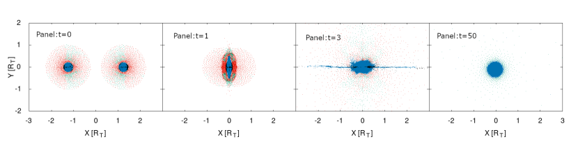
Figure 2: Snapshots of the SPH simulation of a head-on collision with the impact velocity of the mutual escape velocity. From left to right, snapshots show the time at $t=0,1\tau_{\mathrm{ff}},3\tau_{\mathrm{ff}}$, and $50\tau_{\mathrm{ff}}$. Both the target and the impactor have a $1M_{\oplus}$ core with 10 wt% of the H₂ atmosphere. Green and blue particles denote the atmospheric and core components bound on the post-impact planet, respectively. Red and black particles denote the escaping atmospheric and core components, respectively. Both horizontal and vertical axes are normalized by the radius of the target, $R_{\rm T}$.

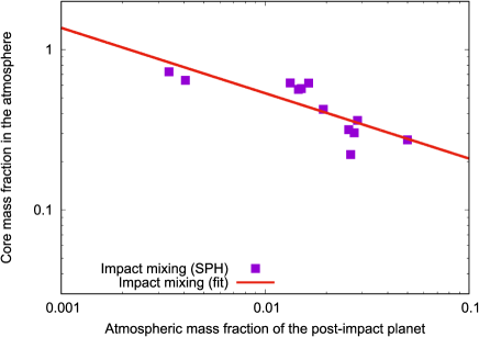
Figure 3: Mass fraction of core material in the remaining atmosphere ($Z_{\mathrm{atm}}$) of an Earth-mass planet after a giant impact. We consider head-on collisions between two Earth-mass planets. The semi-empirical formula of the $Z_{\mathrm{atm}}-X_{\mathrm{atm}}$ relationship obtained from our SPH simulations of giant impacts, $Z_{\mathrm{atm}}=8.2\times 10^{-2}X_{\mathrm{atm}}^{-0.41}$ is also drawn (red line).

3.2 Atmospheric compositions after giant impacts

During a giant impact, vaporized rocky material reacts with the primordial atmosphere. In this section, we focus on chemical reactions between a hydrogen-rich atmosphere and the core material vaporized by the shock of a giant impact. We used ggchem (Woitke et al., 2018) to calculate chemical reactions between the primordial H₂-He gas and rocky vapor, including dust condensation. The primordial atmosphere has the same compositions as the protosolar abundances (Asplund et al., 2021). We consider three kinds of core compositions: basalt (Pierazzo et al., 2005), CI chondrite (Lodders & Palme, 2009), and EH chondrite (Javoy et al., 2010). The elemental abundances of basalt, CI chondrite, and EH chondrite are listed in Table 1.

Element	Protosolar	Basalt	CI	EH
H	7.11E-01	-	1.96E-02	-
He	2.71E-01	-	9.16E-09	-
Li	9.89E-09	-	1.46E-06	-
Be	1.76E-10	-	2.09E-08	-
B	4.47E-09	-	7.74E-07	-
C	2.86E-03	-	3.47E-02	-
N	7.74E-04	-	2.94E-03	-
O	6.41E-03	5.98E-01	4.58E-01	3.11E-01
F	2.05E-07	-	5.81E-05	-
Ne	1.90E-03	-	1.79E-10	-
Na	3.11E-05	1.73E-02	4.98E-03	-
Mg	7.09E-04	3.76E-02	9.67E-02	1.21E-01
Al	5.93E-05	6.13E-02	8.49E-03	9.22E-03
Si	7.50E-04	1.68E-01	1.06E-01	1.90E-01
P	6.50E-06	-	9.66E-04	-
S	3.47E-04	-	5.34E-02	-
Cl	5.93E-06	-	6.97E-04	-
Ar	7.18E-05	-	1.32E-09	-
K	3.76E-06	-	5.43E-04	-
Ca	1.73E-03	5.77E-02	9.21E-03	9.72E-03
Sc	5.07E-08	-	5.89E-06	-
Ti	3.67E-06	5.32E-03	4.50E-04	5.01E-04
V	3.31E-07	-	5.42E-05	-
Cr	1.79E-05	-	2.64E-03	3.61E-03
Mn	1.18E-05	-	1.92E-03	-
Fe	1.33E-03	5.27E-02	1.84E-01	3.31E-01
Co	4.19E-06	-	5.05E-04	1.00E-03
Ni	7.69E-05	-	1.07E-02	2.00E-02

Table 1: Elemental abundances of basalt, CI chondrite, and EH chondrite. The hyphen means the species that are not included in our composition models.

Figure 4 shows the mole fractions of major atomic and molecular species in the primordial atmosphere uniformly mixed with rocky vapor, where the mixing ratio is assumed to be 50%. We also show the mass fractions of six condensates such as MgSiO₃ (enstatite), CaMgSi₂O₆ (diopside), CaAl₂Si₂O₈ (anorthite), and NaAlSi₃O₈ (albite). The atmospheric compositions of an Earth-mass planet in chemical equilibrium have two kinds of regimes: (i) a mineral atmosphere composed of vaporized metal atoms and metal oxides at a high temperature of $\gtrsim$3000 K; and (ii) a volatile-rich atmosphere at a lower temperature. The major components in the low-$T$ atmosphere are H₂, He, and H₂O. Water molecules are produced by reducing FeO by hydrogen at $T\lesssim 3000$ K. The abundance of H₂O is higher than that of CO or CH₄ by two orders of magnitude when the core is composed of basalt or CI chondrite. For the EH-chondrite-like core, the H₂O abundance is comparable to that of CO or CH₄ because oxygen is distributed to dust particles. An Earth-mass planet is likely to have a mineral atmosphere right after a giant impact. As the planet rapidly cools, its atmosphere becomes H₂O-rich because all the metals become dust below $\sim$3000 K and settle into the interior. The mass fractions of H₂ and H₂O vary with the mixing ratio of rocky vapor ($Z_{\mathrm{atm}}$) in the atmosphere of an Earth-mass planet (see Figure 5). As the $Z_{\mathrm{atm}}$ in the atmosphere becomes high, H₂ in the atmosphere is preferentially replaced for H₂O. We also find that the mass fraction of H₂O strongly depends on the core compositions. The water fraction in the impact-generated atmosphere becomes high unless an Earth-mass planet has a reducing core such as EH chondrites.

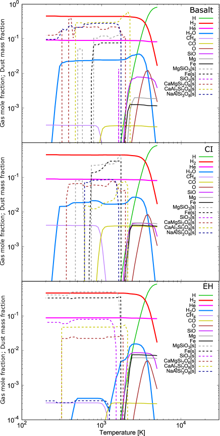
Figure 4: Major species in an 1 bar atmosphere of an Earth-mass planet with three types of core material after a giant impact: basalt (top panel), CI (middle panel), and EH (bottom panel). We assumed that the mixing ratio of rocky vapor to the primordial atmosphere was 50%. Solid and dashed lines show the mole fractions of atomic and molecular species in the gas phase and the mass fractions of dust species, respectively.

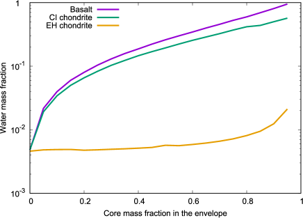
Figure 5: Mass fractions of H₂O at $T=1000$ K in the rock-polluted atmosphere after a giant impact. The purple, green, and orange lines correspond to the case of basalt and CI chondrite, and EH chondrite as core material, respectively.

3.3 Mass loss of the H₂–H₂O atmosphere

In this subsection, we discuss the long-term evolution of a H₂-H₂O atmosphere. The upward transport of H₂O (i.e., $f_{\mathrm{W}}>0$) in the atmosphere via collisions between hydrogen and water occurs while $A_{\mathrm{H}}$ satisfies equation (18). The planet can retain the initial H₂O content if the escape of H₂O is suppressed by inefficient diffusion processes in the atmosphere.

Figure 6 demonstrates the atmospheric evolution of an Earth-mass planet initially having a 6.3 wt% H₂-H₂O atmosphere with a water mole fraction of $A_{\mathrm{W}}=10\%$ at $a=1$ au around a Sun-like star. After a giant impact, the planet cools rapidly and reaches the radiative equilibrium state. The atmospheric escape occurs in two stages in $\gtrsim$10 Myrs. Both hydrogen and water molecules escape as long as the escape flux of hydrogen is high enough to drag oxygen. After $\sim$1000 Myrs, less heavy hydrogen preferentially escapes from the atmosphere by the XUV-driven photoevaporation, whereas H₂O molecules stay in the lower atmosphere. Consequently, as the atmospheric mass decreases, the mole fraction of heavier molecules (H₂O) apparently increases. Thus, the final state of the planetary atmosphere should be enriched in water molecules. In this simulation, the final atmospheric mass fraction is 6.15%, which includes $A_{\rm H}=89.7$ mol% and $A_{\rm W}=10.3$ mol%.

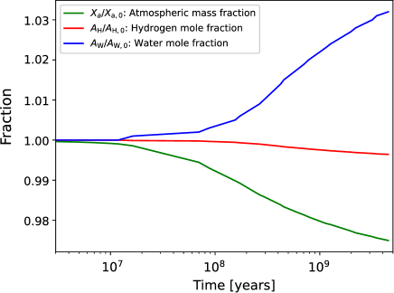
Figure 6: Mole fractions of hydrogen + helium (red line) and water (blue line) in the evaporating atmosphere after a giant impact. We considered an Earth-mass planet that initially has a 6.3 % H₂-H₂O atmosphere with an initial water mole fraction of $A_{\mathrm{W}}=10\,\%$, which is equivalent to a mixing ratio of rocky vapor to H₂-He gas of 90 mol %, at $a=1$ au around a Sun-like star. The planet loses its atmosphere through photoevaporation ($\varepsilon=0.1$) for 4.6 Gyrs. The green line plots the atmospheric mass fraction. The non-smooth features of the blue line is due to the sparse table of H₂O EoS.

3.4 Long-term evolution of the impact-generated atmosphere formed by a giant impact

In Section 3.1, we obtained a semi-empirical scaling law for the initial rock vapor mass fraction in the impact-generated atmosphere (see Figure 3). The water mass fraction ($X_{\mathrm{W}}$) is determined as a function of $X_{\mathrm{atm}}$ shown in Figure 5. We perform the same long-term simulations of an Earth-mass planet with the H₂-H₂O atmosphere using the scaling law as those in Section 3.3. We discuss how the results of Figure 8 change if the $X_{\mathrm{W}}$ is used as the initial condition of the impact-generated atmosphere of an Earth-mass planet. Note that $X_{\mathrm{W}}$ is given by $Z_{\mathrm{atm}}$ shown in figure 5 which is given by the scaling relation of $Z_{\mathrm{atm}}=8.2\times 10^{-2}X_{\mathrm{atm}}^{-0.41}$.

The left, middle, and right panels of Figure 7 show the relationship between the initial ($X_{\mathrm{atm},0}$: top) and final ($X_{\mathrm{atm}}$: bottom) atmospheric mass fraction of an Earth-mass planet and the water mole fraction in the remaining atmosphere after the atmospheric loss through photoevaporation over 4.6 Gyr for core models with the basalt, CI, and EH compositions, respectively. A water-dominated atmosphere is more likely to form in a less massive atmosphere after a giant impact; the mole fraction of water remaining in the atmosphere exceeds 10 % when $X_{\mathrm{atm}}\leq 4\times 10^{-3}$ for the case of a basalt core model and $X_{\mathrm{atm}}\leq\times 10^{-3}$ for the case of a CI-chondritic core one. In contrast, such a water-rich atmosphere is difficult for an Earth-mass planet with a reducing core like an EH chondrite to form. We find that an Earth-mass planet requires an oxidizing core to produce a water-rich atmosphere in the giant impact scenario, followed by the atmospheric escape.

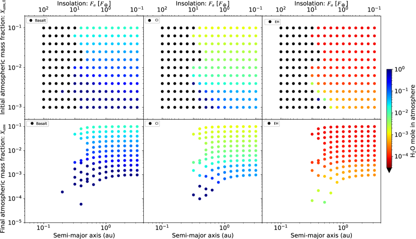
Figure 7: Initial and final atmospheric mass fraction $X_{\mathrm{atm}}$ and final water mole fraction (color bar) after the atmospheric loss through photoevaporation ($\varepsilon=0.1$) for 4.6 Gyrs. The rocky core is composed of basalt (left panel), CI (middle panel), and EH (right panel). An initial water mass fraction is determined by the empirical relation derived from the giant impact simulations, $X_{\mathrm{W}}=8.2\times 10^{-2}X_{\mathrm{atm}}^{-0.41}$. The color contour shows the final H₂O mole fraction in the remaining atmosphere.

4 Discussion

We see the dependence of the final atmospheric water fraction on the semi-major axis and the initial water content (Section 4.1). We also present the analytical condition for the water-dominated atmosphere (Section 4.2), and discuss the caveats of our models (Section 4.3).

4.1 Dependence of the final atmospheric water fraction on the semi-major axis and the initial water content

We examine how mass loss affects the water fractions in the atmospheres of Earth-mass planets after giant impacts with various semimajor axes and initial water content. We consider that the initial atmospheric mass fraction relative to the total mass of a planet ranges from $10^{-3}$ to $10^{-1}$. The initial H₂O mole fractions in the atmosphere $A_{\mathrm{W}}$ are assumed to be 1%, 3%, and 10%. Figure 8 shows the initial and final atmospheric mass fractions and the final water mole fraction in the atmosphere of an Earth-mass planet with a given equilibrium temperature after $t=4.6~{}$ Gyrs.

There are three key parameters for the survival of the water-rich atmosphere of an Earth-mass planet: the semimajor axis of the planet, $a$, the initial water mole fraction in the atmosphere, $A_{\mathrm{W}}$, and the initial atmospheric mass, $X_{\mathrm{atm}}$. When the planet is close to its host star, it loses almost all of its H₂-H₂O atmosphere and becomes a bare rocky planet. If the planet is distant from its star and exposed to less intensive XUV irradiation, neither its atmospheric mass $X_{\mathrm{atm}}$ nor its water mole fraction $A_{\mathrm{W}}$ changes significantly. In this case, the final water mole fraction in the atmosphere reflects the initial water content that the planet has formed. Water molecules tend to remain in the atmosphere if the atmospheric mass fraction is less than about 0.3%. The initial atmosphere with a higher initial $A_{\mathrm{W}}$ is likely to survive because a low escape flux of hydrogen in the water-rich atmosphere reduces the efficiency of the upward transport of water molecules.

The XUV-driven atmospheric escape of an Earth-mass planet yields a high H₂O abundance in the atmosphere for planets with $X^{\mathrm{initial}}_{\mathrm{atm}}\lesssim$ 0.3% ($X^{\mathrm{final}}_{\mathrm{atm}}<$ 0.1%) when it receives $F_{\mathrm{a}}>2F_{\oplus}$. Such a planet should have a steam atmosphere because its insolation exceeds the critical flux for a runaway greenhouse effect around a Sun-like star (e.g. Kopparapu et al., 2014; Kodama et al., 2019). The less efficient heating of hydrogen by UV photons (e.g., $\varepsilon=0.01$) moves the outer edge of a “steamy zone” closer to a central star (see also Figure 9).

One of the key findings of the present study is that the enhancement of H₂O in the atmosphere of an Earth-mass planet occurs if $f_{\mathrm{W}}=0$, i.e., in the case that only hydrogen escapes. Unless a planet loses its atmosphere completely, a low escape flux of hydrogen in a less massive H₂–H₂O atmosphere that satisfies $f_{\mathrm{W}}=0$ forms a water-dominated atmosphere in Gyrs. In Section 4.2, we analytically derive the condition for the formation of a water-dominated atmosphere of an Earth-mass planet. Also, as we will see in Section 3.4, even when the results of giant impact simulations are taken into account, there is no change in this finding.

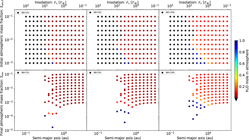
Figure 8: Same as Figure 7 but with different initial water mole fractions (1%, 3%, and 10% in the left, middle, and right panels, respectively). The rocky core is assumed to be basalt in all simulations.

4.2 Analytical condition for the water-dominated atmosphere

In Section 3.3, we demonstrate that the Earth-mass planet with a small atmospheric mass fraction at $a=1$ au has a water-dominated atmosphere in Gyrs. We analytically derive the condition in which Earth-mass planets have water-dominated atmospheres.

The outflow of escaping hydrogen cannot drive the escape of water molecules if $f_{\mathrm{W}}=0$, that is, $f_{\mathrm{H}}\leq f^{\mathrm{crit}}_{\mathrm{H}}$ (see equation (18)). The mass loss process increases the H₂O mole fraction when $f_{\mathrm{H}}\leq f^{\mathrm{crit}}_{\mathrm{H}}$. Integrating equation (21) from $t=0$ to $t=\Delta t$, we obtain the upper-limit mass fraction of H₂ and He in the impact-generated atmosphere in which all water molecules can persist for $\Delta t$;

$$X^{\mathrm{max}}_{\mathrm{H}}\equiv\frac{M_{\mathrm{esc}}}{M_{\mathrm{p}}(t=0)}=\frac{4\pi Gbm_{\mathrm{H}_{2}}\Delta m}{k_{\mathrm{B}}T}A_{\mathrm{H}}(t=0)\Delta t,$$ (28)

where $M_{\mathrm{esc}}$ is the net mass loss of a H₂-He atmosphere. This value is given by $M_{\mathrm{esc}}=\int\frac{dM_{\mathrm{esc}}}{dt}dt\approx 3\varepsilon\bar{F}\Delta t/(4G\bar{\rho}_{\mathrm{p}})$, where $\bar{F}=\int F_{\mathrm{XUV}}dt$ and $\bar{\rho}_{p}$ is the planetary mean density. An Earth-mass planet can have a water-dominated atmosphere if it initially has an impact-generated atmosphere of $X_{\mathrm{H}}\leq X^{\mathrm{max}}_{\mathrm{H}}$. The condition for a water-dominated atmosphere of a planet, $X^{\mathrm{max}}_{\mathrm{H}}$, well explains our numerical results as shown in Figure 8. In fact, Earth-mass planets with water-dominated atmospheres appear just below the criterion of $X^{\mathrm{max}}_{\mathrm{H}}$ after 4.6 Gyrs unless such planets lose their atmospheres completely by photoevaporation after a giant impact.

Next, we consider the range of semimajor axes in which Earth-mass planets with water-dominated atmospheres can exist. We can obtain the approximate semimajor axis within which a planet loses all of its the H₂/He, $a_{\mathrm{esc}}$:

$$a_{\mathrm{esc}}=\left(\frac{3}{4G}\frac{\overline{\epsilon L_{\mathrm{XUV}}}\Delta t}{M_{\mathrm{p}}\rho_{p}X_{\mathrm{atm}}}\right)^{\frac{1}{2}},$$ (29)

where $\Delta t$ is the time elapsed after a giant impact, $M_{\mathrm{atm}}$ is the atmospheric mass of a planet, $\rho_{\mathrm{p}}$ is the mean density of a planet, and $\overline{\epsilon L_{\mathrm{XUV}}}$ is the time-averaged XUV luminosity that a planet receives. Note that $K_{\mathrm{tide}}\sim 1$ for an Earth-mass planet in this study. A large hydrogen flux causes the escaping flow of water molecules, namely when $f_{\mathrm{H}}>f^{\mathrm{crit}}_{\mathrm{H}}$ (see equation (18)). The farther a planet is from a central star, the lower the escape rate of hydrogen becomes under stellar XUV irradiation. The critical semimajor axis ($a_{\mathrm{W}}$) beyond which an Earth-mass planet prevents the threat of H₂O escape is defined by $f_{\mathrm{H}}=f^{\mathrm{crit}}_{\mathrm{H}}$;

$$a_{\mathrm{W}}=\sqrt{\frac{3}{4G}\frac{\overline{\epsilon L_{\mathrm{XUV}}}}{\rho_{p}}\frac{k_{B}T_{\mathrm{atm}}}{4\pi m_{H}^{2}A_{H}GM_{p}b(T_{\mathrm{atm}})}},$$ (30)

where $T_{\mathrm{atm}}$ is the atmospheric temperature. If $a_{\mathrm{W}}<a<a_{\mathrm{esc}}$, the planet undergoes the hydrodynamic escape of hydrogen, but it preserves the initial amount of water in the atmosphere.

Figure 9 shows the habitat of an Earth-mass planet that has a water-dominated atmosphere (i.e., $a_{\mathrm{W}}<a<a_{\mathrm{esc}}$, hereafter the steamy zone”). We set $\overline{L_{\mathrm{XUV}}}=3.1\times 10^{28}~{}\mathrm{erg}\cdot\mathrm{s}^{-1}$ for a Sun-like star and $T_{\mathrm{atm}}=500~{}$K. Since the atmospheric temperature at the upper stratosphere is higher than the equilibrium temperature, we assume that $T_{\mathrm{atm}}$ is determined by the planet’s atmosphere at typically $10^{8}$ years old. The XUV heating efficiency, $\varepsilon$, determines the inner and outer edges of a steamy Earth-mass planet. The formation of a steam atmosphere requires the initial atmosphere mass fraction $X_{\mathrm{atm}}\lesssim 2\times 10^{-3}$ regardless of $\varepsilon$. These “steamy zones” are in good agreement with the results shown in Figure 8.

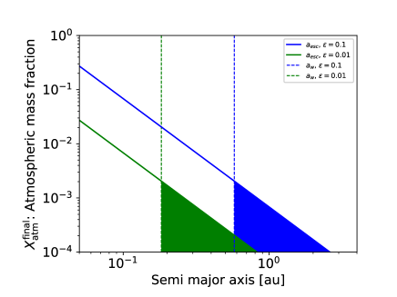
Figure 9: Habitat of an Earth-mass planet with a water-rich atmosphere that orbits a Sun-like star. Dashed and solid lines represent $a_{\mathrm{esc}}$ (Eq. 29) and $a_{\mathrm{W}}$ (Eq. 30) in two models with $\varepsilon=0.1$ (blue) and $0.01$ (green), respectively. Blue and green shaded regions show the conditions where an Earth-mass planet can retain water in the atmosphere for Gyrs.

4.3 Caveats

This study considered a head-on giant impact on an Earth-mass planet. In reality, grazing impacts occur in the final stage of terrestrial planet formation (e.g., Kokubo & Genda, 2010; Ogihara et al., 2020). Less efficient mixing of a H₂/He atmosphere and vaporized core material by oblique collisions decreases the production of H₂O. We also assumed simple rock compositions for core material. If the core of an Earth-mass planet is a mixture of icy and rocky material, the chemical compositions of an impact-generated atmosphere become different. Moreover, dust clouds may form in the polluted atmosphere unless dust particles fall into the deep interior.

The atmospheric compositions generated by the impact are still debated. Lupu et al. (2014) showed that a post-impact planetary atmosphere is dominated by CO₂ as well as H₂O. We should underestimate the abundance of carbon-bearing species since the rock material is assumed to be carbon-depleted. The mass loss efficiency in our study may be overestimated because CO₂ helps to cool the upper atmosphere (Yoshida & Kuramoto, 2020). Another caveat involves the mixing rate of rock material in the primordial atmosphere. We considered only head-on collisions, which cause the most efficient mixing between the atmosphere and the rock vapor, as indicated by the Moon-forming impact simulations on the proto-Earth (Nakajima & Stevenson, 2015). The present study focused on the most optimistic case, where a giant impact into an Earth-sized planet forms a water-rich atmosphere. Detailed atmospheric compositions of Earth-sized planets after a non-oblique giant impact will be discussed in our future work.

5 conclusion

We showed that the mixing of hydrogen in the atmosphere and rocky material vaporized by a giant impact into an Earth-sized planet results in the production of H₂O via chemical reactions. We simulated the long-term evolution of the H₂-H₂O atmospheres of Earth-mass planets around a Sun-like star for Gyrs after giant impacts. We examined the mass loss from an Earth-sized planet that initially has a H₂-H₂O atmosphere of 0.1 wt% – 10 wt% at a semimajor axis from 0.1 to 3 au. Our key findings are summarized as follows.

• The composition of the impact-generated atmosphere is dominated by H₂, He, and H₂O when it has cooled below 3000 K.

• Earth-mass planets can avoid water loss through photoevaporation if the escape flux of hydrogen is too low to drag oxygen via collisions.

• The post-impact atmosphere of an Earth-mass planet evolves into a water-dominated atmosphere if its atmospheric mass fraction is less than a few times 0.1% provided that the core is oxidizing material such as the basalt or CI chondrite.

• If the rocky core is composed of a reducing material such as EH chondrite, the post-impact atmosphere should not be water-dominated, even if the impact-induced mixing between H₂-He gas and rocky vapor is efficient.

An Earth-mass planet in a habitable zone can retain the initial amount of H₂O in its atmosphere if $X_{\mathrm{atm}}^{\mathrm{final}}\lesssim 10^{-3}$ after a giant impact, although part of the remaining water exists as “oxygen” in the atmosphere due to photodissociation. Note that the water-rich atmosphere of an Earth-mass planet can be found on the core composed of basalt and CI chondrite in the giant impact scenario, while the water-poor atmosphere forms on the core composed of EH chondrite. The advanced capability of the James-Webb space telescope (JWST) allows it to observe the atmospheres of Earth-sized planets around nearby stars, e.g., TRAPPIST-1 planets (Lustig-Yaeger et al., 2019). In the late 2020s, PLATO (Rauer et al., 2014), Earth 2.0 (Ge et al., 2022), and the Roman space telescope (Penny et al., 2019) are expected to find hundreds of Earth-sized planets in a habitable zone around Sun-like stars and M-dwarfs. Terrestrial planets with water-dominated atmospheres, as considered in this study, should be interesting targets for JWST observations. As shown in Figure 7, such terrestrial planets can exist in orbits of semimajor axes ranging from a few 0.1 au to a few au, depending on the photoevaporation efficiency ($\varepsilon$). This constraint on the locations of terrestrial planets with water-dominated atmospheres helps elucidate the mass-loss efficiency.

References

- Abe & Matsui (1988) Abe, Y., & Matsui, T. 1988, Journal of Atmospheric Sciences, 45, 3081
- Ahrens (1993) Ahrens, T. J. 1993, Annual Review of Earth and Planetary Sciences, 21, 525, doi: 10.1146/annurev.ea.21.050193.002521
- Asplund et al. (2021) Asplund, M., Amarsi, A. M., & Grevesse, N. 2021, A&A, 653, A141, doi: 10.1051/0004-6361/202140445
- Atreya (1986) Atreya, S. K. 1986, Atmospheres and Ionospheres of the Outer Planets and their Satellites (Springer)
- Chamberlain & Hunten (1987) Chamberlain, J., & Hunten, D. 1987, Orlando.[Google Scholar]
- Denman et al. (2022) Denman, T. R., Leinhardt, Z. M., & Carter, P. J. 2022, MNRAS, 513, 1680, doi: 10.1093/mnras/stac923
- Dressing & Charbonneau (2015) Dressing, C. D., & Charbonneau, D. 2015, ApJ, 807, 45, doi: 10.1088/0004-637X/807/1/45
- Erkaev et al. (2007) Erkaev, N. V., Kulikov, Y. N., Lammer, H., et al. 2007, A&A, 472, 329, doi: 10.1051/0004-6361:20066929
- Freedman et al. (2008) Freedman, R. S., Marley, M. S., & Lodders, K. 2008, ApJS, 174, 504, doi: 10.1086/521793
- Fulton & Petigura (2018) Fulton, B. J., & Petigura, E. A. 2018, AJ, 156, 264, doi: 10.3847/1538-3881/aae828
- Ge et al. (2022) Ge, J., Zhang, H., Zang, W., et al. 2022, arXiv e-prints, arXiv:2206.06693. https://arxiv.org/abs/2206.06693
- Genda & Abe (2003) Genda, H., & Abe, Y. 2003, Icarus, 164, 149, doi: 10.1016/S0019-1035(03)00101-5
- Gordon et al. (2022) Gordon, I. E., Rothman, L. S., Hargreaves, R. J., et al. 2022, J. Quant. Spec. Radiat. Transf., 277, 107949, doi: 10.1016/j.jqsrt.2021.107949
- Guillot (2010) Guillot, T. 2010, A&A, 520, A27, doi: 10.1051/0004-6361/200913396
- Hamano et al. (2013) Hamano, K., Abe, Y., & Genda, H. 2013, Nature, 497, 607, doi: 10.1038/nature12163
- Hirano et al. (2018) Hirano, T., Dai, F., Gandolfi, D., et al. 2018, AJ, 155, 127, doi: 10.3847/1538-3881/aaa9c1
- Hori & Ogihara (2020) Hori, Y., & Ogihara, M. 2020, ApJ, 889, 77, doi: 10.3847/1538-4357/ab6168
- Hunten et al. (1987) Hunten, D. M., Pepin, R. O., & Walker, J. C. G. 1987, Icarus, 69, 532, doi: 10.1016/0019-1035(87)90022-4
- Ikoma & Genda (2006) Ikoma, M., & Genda, H. 2006, ApJ, 648, 696, doi: 10.1086/505780
- Ikoma & Hori (2012) Ikoma, M., & Hori, Y. 2012, ApJ, 753, 66, doi: 10.1088/0004-637X/753/1/66
- Ingersoll (1969) Ingersoll, A. P. 1969, Journal of Atmospheric Sciences, 26, 1191
- Itcovitz et al. (2022) Itcovitz, J. P., Rae, A. S. P., Citron, R. I., et al. 2022, arXiv e-prints, arXiv:2204.09946. https://arxiv.org/abs/2204.09946
- Javoy et al. (2010) Javoy, M., Kaminski, E., Guyot, F., et al. 2010, Earth and Planetary Science Letters, 293, 259, doi: 10.1016/j.epsl.2010.02.033
- Johnstone (2020) Johnstone, C. P. 2020, ApJ, 890, 79, doi: 10.3847/1538-4357/ab6224
- Kegerreis et al. (2020) Kegerreis, J. A., Eke, V. R., Catling, D. C., et al. 2020, ApJ, 901, L31, doi: 10.3847/2041-8213/abb5fb
- Kodama et al. (2019) Kodama, T., Genda, H., O’ishi, R., Abe-Ouchi, A., & Abe, Y. 2019, Journal of Geophysical Research (Planets), 124, 2306, doi: 10.1029/2019JE006037
- Kokubo & Genda (2010) Kokubo, E., & Genda, H. 2010, ApJ, 714, L21, doi: 10.1088/2041-8205/714/1/L21
- Kopparapu et al. (2014) Kopparapu, R. K., Ramirez, R. M., SchottelKotte, J., et al. 2014, ApJ, 787, L29, doi: 10.1088/2041-8205/787/2/L29
- Kurosaki & Ikoma (2017) Kurosaki, K., & Ikoma, M. 2017, AJ, 153, 260, doi: 10.3847/1538-3881/aa6faf
- Kurosaki et al. (2014) Kurosaki, K., Ikoma, M., & Hori, Y. 2014, A&A, 562, A80, doi: 10.1051/0004-6361/201322258
- Kurosaki & Inutsuka (2023) Kurosaki, K., & Inutsuka, S.-i. 2023, arXiv e-prints, arXiv:2307.12782, doi: 10.48550/arXiv.2307.12782
- Lammer et al. (2013) Lammer, H., Chassefière, E., Karatekin, Ö., et al. 2013, Space Sci. Rev., 174, 113, doi: 10.1007/s11214-012-9943-8
- Lange & Ahrens (1982) Lange, M. A., & Ahrens, T. J. 1982, Icarus, 51, 96, doi: 10.1016/0019-1035(82)90031-8
- Lee et al. (2018) Lee, E. J., Chiang, E., & Ferguson, J. W. 2018, MNRAS, 476, 2199, doi: 10.1093/mnras/sty389
- Lichtenberg et al. (2022) Lichtenberg, T., Schaefer, L. K., Nakajima, M., & Fischer, R. A. 2022, arXiv e-prints, arXiv:2203.10023, doi: 10.48550/arXiv.2203.10023
- Lodders & Palme (2009) Lodders, K., & Palme, H. 2009, Meteoritics and Planetary Science Supplement, 72, 5154
- Lopez & Fortney (2014) Lopez, E. D., & Fortney, J. J. 2014, ApJ, 792, 1, doi: 10.1088/0004-637X/792/1/1
- Lupu et al. (2014) Lupu, R. E., Zahnle, K., Marley, M. S., et al. 2014, ApJ, 784, 27, doi: 10.1088/0004-637X/784/1/27
- Lustig-Yaeger et al. (2019) Lustig-Yaeger, J., Meadows, V. S., & Lincowski, A. P. 2019, AJ, 158, 27, doi: 10.3847/1538-3881/ab21e0
- Matsui & Abe (1986) Matsui, T., & Abe, Y. 1986, Nature, 319, 303, doi: 10.1038/319303a0
- Maurice et al. (2023) Maurice, M., Dasgupta, R., & Hassanzadeh, P. 2023, arXiv e-prints, arXiv:2301.07505. https://arxiv.org/abs/2301.07505
- Melosh (2007) Melosh, H. J. 2007, \maps, 42, 2079, doi: 10.1111/j.1945-5100.2007.tb01009.x
- Nakajima & Stevenson (2015) Nakajima, M., & Stevenson, D. J. 2015, Earth and Planetary Science Letters, 427, 286, doi: 10.1016/j.epsl.2015.06.023
- Ogihara et al. (2020) Ogihara, M., Kunitomo, M., & Hori, Y. 2020, ApJ, 899, 91, doi: 10.3847/1538-4357/aba75e
- Owen & Wu (2013) Owen, J. E., & Wu, Y. 2013, ApJ, 775, 105, doi: 10.1088/0004-637X/775/2/105
- Penny et al. (2019) Penny, M. T., Gaudi, B. S., Kerins, E., et al. 2019, ApJS, 241, 3, doi: 10.3847/1538-4365/aafb69
- Petigura et al. (2013) Petigura, E. A., Howard, A. W., & Marcy, G. W. 2013, Proceedings of the National Academy of Science, 110, 19273, doi: 10.1073/pnas.1319909110
- Pierazzo et al. (2005) Pierazzo, E., Artemieva, N. A., & Ivanov, B. A. 2005, Geological Society of America Special Paper, 384, 443, doi: 10.1130/0-8137-2384-1.443
- Rauer et al. (2014) Rauer, H., Catala, C., Aerts, C., et al. 2014, Experimental Astronomy, 38, 249, doi: 10.1007/s10686-014-9383-4
- Ribas et al. (2005) Ribas, I., Guinan, E. F., Güdel, M., & Audard, M. 2005, ApJ, 622, 680, doi: 10.1086/427977
- Rogers (2015) Rogers, L. A. 2015, ApJ, 801, 41, doi: 10.1088/0004-637X/801/1/41
- Rothman et al. (1998) Rothman, L. S., Rinsland, C. P., Goldman, A., et al. 1998, J. Quant. Spec. Radiat. Transf., 60, 665, doi: 10.1016/S0022-4073(98)00078-8
- Saumon et al. (1995) Saumon, D., Chabrier, G., & van Horn, H. M. 1995, ApJS, 99, 713, doi: 10.1086/192204
- Schlichting et al. (2015) Schlichting, H. E., Sari, R., & Yalinewich, A. 2015, Icarus, 247, 81, doi: 10.1016/j.icarus.2014.09.053
- Thompson & Lauson (1972) Thompson, S. L., & Lauson, H. S. 1972, Improvements in the Chart D Radiation-Hydrodynamic Code. III: Revised Analytic Equations of State, Albuquerque, New Mexico: Sandia National Laboratory. 1972. Technical Report SC-RR-71-0714
- Thompson et al. (2019) Thompson, S. L., Lauson, H. S., Melosh, H. J., Collins, G. S., & Stewart, S. T. 2019, M-ANEOS, 1.0, Zenodo, Zenodo, doi: 10.5281/zenodo.3525030
- Weiss & Marcy (2014) Weiss, L. M., & Marcy, G. W. 2014, ApJ, 783, L6, doi: 10.1088/2041-8205/783/1/L6
- Woitke et al. (2018) Woitke, P., Helling, C., Hunter, G. H., et al. 2018, A&A, 614, A1, doi: 10.1051/0004-6361/201732193
- Yelle et al. (2008) Yelle, R., Lammer, H., & Ip, W.-H. 2008, Space Sci. Rev., 139, 437, doi: 10.1007/s11214-008-9420-6
- Yoshida & Kuramoto (2020) Yoshida, T., & Kuramoto, K. 2020, Icarus, 345, 113740, doi: 10.1016/j.icarus.2020.113740
- Yoshida & Kuramoto (2021) —. 2021, MNRAS, 505, 2941, doi: 10.1093/mnras/stab1471
- Yoshida et al. (2022) Yoshida, T., Terada, N., Ikoma, M., & Kuramoto, K. 2022, ApJ, 934, 137, doi: 10.3847/1538-4357/ac7be7
- Zahnle et al. (1988) Zahnle, K. J., Kasting, J. F., & Pollack, J. B. 1988, Icarus, 74, 62, doi: 10.1016/0019-1035(88)90031-0
- Zeng et al. (2019) Zeng, L., Jacobsen, S. B., Sasselov, D. D., et al. 2019, Proceedings of the National Academy of Science, 116, 9723, doi: 10.1073/pnas.1812905116