Identifying confounders in deep-learning-based model predictions using DeepRepViz

Abstract

Deep Learning (DL) models are increasingly used to analyze neuroimaging data and uncover insights about the brain, brain pathologies, and psychological traits. However, extraneous ‘confounders’ variables such as the age of the participants, sex, or imaging artifacts can bias model predictions, preventing the models from learning relevant brain-phenotype relationships. In this study, we provide a solution called the ‘DeepRepViz’ framework that enables researchers to systematically detect confounders in their DL model predictions. The framework consists of (1) a metric that quantifies the effect of potential confounders and (2) a visualization tool that allows researchers to qualitatively inspect what the DL model is learning. By performing experiments on simulated and neuroimaging datasets, we demonstrate the benefits of using DeepRepViz in combination with DL models. For example, experiments on the neuroimaging datasets reveal that sex is a significant confounder in a DL model predicting chronic alcohol users (Con-score=0.35). Similarly, DeepRepViz identifies age as a confounder in a DL model predicting participants’ performance on a cognitive task (Con-score=0.3). Overall, DeepRepViz enables researchers to systematically test for potential confounders and expose DL models that rely on extraneous information such as age, sex, or imaging artifacts.

Introduction

Deep learning (DL) models demonstrate a capability to discover complex, non-linear patterns from high-dimensional ($p>>n$) data [6]. Hence, DL is becoming a popular choice for analyzing neuroimaging data such as Magnetic Resonance Imaging (MRI). Specifically in population neuroscience studies [15], DL models are used to uncover relationships between the brain and psychological behaviors, cognitive traits, and brain pathologies on large observational neuroimaging datasets ($n>1000$) [27, 4]. For example, DL models are trained on brain MRI data to diagnose Alzheimer’s disease (AD) [10] or to predict chronic alcohol misuse behavior [17]. If such models achieve a significantly high accuracy then this can imply the potential existence of biomarkers of AD or alcohol misuse in the brain. However, high accuracy in such brain-phenotype prediction tasks can also be caused by the presence of certain extraneous variables called ‘confounders’ that are prevalent in observational datasets [16]. Some examples of such confounders include the age or sex of the participants, or imaging artifacts added during the data acquisition process. Confounders can prevent predictive models from discovering useful brain-phenotype relationships (e.g. neurological biomarkers of AD) [9]. Thus, confounders pose a major hurdle for using predictive models with observational neuroimaging datasets [4].

Studies routinely report that confounders contaminate their model predictions [9, 1, 22, 26, 19]. Theoretically, a confounder is defined as follows. In a prediction task $f_{\theta}:X\mapsto y$, there can exist certain extraneous variables $c^{k}$ that are encoded in the exposure $X$ (ex: neuroimaging) and also associated with the outcome $y$. This creates an alternative prediction pathway $X\leftmapsto c^{k}\mapsto y$ [19] mediated by the variable $c^{k}$. $c^{k}$ is defined as a ‘confounder’ in the prediction task if the pathway $X\leftmapsto c^{k}\mapsto y$ prevents the model $f_{\theta}$ from generalizing to the intended application of the model [19]. For example, a DL model trained on structural MRI data to predict the development of AD was found to be confounded by the magnetic field strength of the MRI scanners (SS) [26]. This was caused by a systematic data acquisition bias [3] present in the dataset. The majority of the participants in their dataset that developed AD were scanned using a 3 Tesla MRI scanner, whereas the majority of controls were scanned using a 1.5 Tesla scanner [26]. The DL model exploited the relationship $MRI\leftmapsto SS\mapsto AD$ as a proxy for predicting AD. The age of the participants can also be a confounder when diagnosing AD [16]. Higher brain atrophies linked with AD are also more prevalent among older participants [8]. If a model exploits the relationship $atrophy\leftmapsto age\mapsto AD$ and always diagnoses older participants as having AD, then such a model would not be clinically valid.

The effect of confounders can be controlled to an extent using confound control or ‘deconfounding’ methods [20]. For example, one can regress out the information related to the confounder from the neuroimaging data [23] or remove the correlation between the confounder and the predicted phenotype by systematically resampling the dataset [19]. Generally in neuroimaging studies, researchers choose 2 to 5 variables as potential confounders in their analyses [9] and control for them using standard deconfounding methods [23, 19]. For example, these include age, sex, intracranial brain volume, educational level, and the socio-economic status of the participants. However, the variables that must be considered as confounders depend on the specific research question. Confounders are also dependant on the particular dataset used in the study as they can stem from sampling biases present in the dataset [3]. Therefore, choosing a fixed set of confounder variables in all neuroimaging studies without taking into consideration factors such as the specific research question or dataset biases is considered a poor study design [16, 9].

Sometimes, the confounders that are corrected in a study can have a more significant influence on the model performance than even the choice of the modeling algorithm [19, 18], or the input neuroimaging modality [9, 12]. Therefore, it is recommended to systematically test all potential confounders in the dataset [7, 24] and ensure that are accounted for in the analysis. One way to achieve this is by checking if the confounder pathway $X\leftmapsto c^{k}\mapsto y$ exists for each potential confounder $c^{k}$ [19]. Indeed, [19] implemented such a ‘confounder identification test’ for classical machine learning models such as Logistic Regression and Support Vector Machine. Using the same machine learning pipeline used to predict $X\mapsto y$ [7], they also estimate $X\mapsto c^{k}$ and $c^{k}\mapsto y$ and check if both the prediction accuracies are significant. If yes, then they consider $c^{k}$ as a potential confounder. They apply a deconfounding method on $c^{k}$ and ensure that the pathway $X\leftmapsto c^{k}\mapsto y$ is destroyed. In this study, we develop a similar confounders identification test that can be applied to DL models.

Our proposed solution is called the ‘DeepRepViz’ framework. DeepRepViz consists of a metric we call ‘Con-score’ that quantifies if a confounder pathway $X\leftmapsto c^{k}\mapsto y$ is present in a DL model prediction. We estimate this in the latent representation learned by the DL model in its final layer. Additionally, DeepRepViz consists of a web-based visualization tool. The tool enables researchers to qualitatively inspect the latent representation learned by their model [2] for signs of confounders. In the following sections, we will demonstrate how the DeepRepViz framework helps to identify confounders in DL model predictions.

Method

We will now provide some theoretical background. Consider the DL model $f_{model}$ in Figure 1 (a) that is performing the prediction $X_{i}\mapsto y_{i}$, where $i\in\{1,2,...n\}$ represents one sample in the dataset of $n$ samples . According to the representation learning theory [2], the model can be imagined to be formed of 2 stages, $X_{i}\mapsto^{nonlinear}h_{i}^{(l-1)}\mapsto^{linear}\hat{y_{i}}$. That is, all the layers from the first until the penultimate layer learn a non-linear mapping $h^{(l-1)}_{i}$ of the input $X_{i}$ [2]. Therefore, $H^{l-1}=\{h_{i}^{(l-1)}\;|\;i\in 1,2,...n\}$ is the condensed latent representation learned by the DL model for all data points in the training dataset. The purpose of the final layer is to learn a linear mapping from $h_{i}^{(l-1)}$ to the label $y_{i}$. From a representation learning perspective, the layer learns a linear decision boundary on the latent representation $H^{l-1}$ to predict the label $y$ . If $y$ is a continuous variable, the final layer performs a linear regression instead.

We propose performing a confounder identification test on the final non-linear representation learned by the DL model $H^{l-1}$. If we expect that the DL model uses the alternative confounder pathway $X\leftmapsto c^{k}\mapsto y$ for making its predictions then we would expect two things to be true [19]. Firstly, $c^{k}$ is linearly predictable from $H^{l-1}$, i.e. $X\mapsto H^{l-1}\mapsto c^{k}$ exists. Secondly, the linear prediction of $c^{k}$ corresponds with the linear prediction of $y$ by the the final layer of the DL model. Building upon this rationale, we propose a metric called ‘Con-score’ as given in Equation 1 :

$$\text{Con-score}\,(c^{k})=\>R_{c^{k}}^{2}\cdot\,|\,\cos\,(\theta_{cy})$$ (1)

where $R_{c^{k}}^{2}$ is the coefficient of multiple determination [14] and

$$\cos(\theta_{cy})$$

is the cosine similarity between the linear model predicting $c^{k}$ and the linear DL layer predicting $y$. Specifically, the first term $R_{c^{k}}^{2}$ is the performance of the linear predictive model $H^{l-1}\mapsto c^{k}$ and its values lie between $[0,1]$ [14]. If $c^{k}$ is categorical then McKelvey and Zavoinas pseudo $R^{2}$ [13] is used to estimate the performance instead of the coefficient of multiple determination. In the second term, the $\theta_{cy}$ is obtained by taking the vector angle between the parameter of the linear model predicting $H^{l-1}\mapsto c^{k}$ and the parameters of the last DL layer performing the linear prediction $H^{l-1}\mapsto y$. The final Con-score ranges between $[0,1]$. The higher the Con-score, the higher is the likelihood that the model is using the alternative (confounder) pathway $H^{l-1}\leftmapsto c^{k}\mapsto y$ for its prediction. A Con-score of 1 indicates that the DL model has learned all information about $c_{k}$ in $H^{l-1}$, and that the linear prediction of $y$ and the linear prediction of $c_{k}$ are exactly the same.

Visualization tool: When training a DL model for a brain-phenotype prediction, we can simultaneously estimate the Con-score for all variables present in the neuroimaging dataset, such as the MRI scanning parameters, demographics, or socio-economic status of the participants [7, 18]. The visualization tool enables researchers to additionally inspect the learned representation of the DL model $H^{l-1}$ qualitatively. If the Con-score is high for $c^{k}$ then we can expect $c^{k}$ to be clustered in the representation space $H^{l-1}$[5] similar to the predicted $\hat{y}$. As an example, in Figure 1, we demonstrate how the visualization tool helps to identify that the sex of the participants is a confounder in the prediction of chronic alcohol use from brain MRI.

Experiment design: We first validate the Con-score on simulated data. Here, we test how the metric performs under controlled settings and for different boundary conditions. Next, we evaluate the utility of the Con-score metric and the visualization tool on three brain-phenotype prediction tasks representative of common population neuroscience studies [19, 28].

(a) Simulated data: The simulated dataset consists of a binary label $y$, a binary confounder $c$, and a 2-dimensional input data $H=\{h_{0},h_{1}\}$. We generate eight instances of the simulated dataset by systematically changing the correlation between $y$, $c$, and the input data $H$. The scatterplots in Figure 2 (a) show all eight instances. In the figure, the binary states of the label $y$ are represented with different colors, whereas the binary states of the confounder $c$ are represented by different shapes, as enlisted in the figure legend. In the dataset instances on the top row (numbered 1 to 4), we sample the input features $H$ and the confounder $c$ such that $c$ is easily predictable with a linear classification model. In contrast, we generate the instances on the bottom row (5 to 8) such that it is relatively harder to classify $c$. As we move from instance number 1 to 4 or from 5 to 8, we can see that the correlation between $c$ and $y$ changes incrementally. For example, in the instance number 1, $c$ and $y$ are completely uncorrelated, but as we move to the instance 3, $c$ becomes completely correlated with $y$.

(b) Neuroimaging data: On a subsample of the UK Biobank dataset [25] ($n=12000$), we perform three exemplary brain-phenotype prediction tasks using DL. Using the T1-weighted structural MRI data, we predict the participant’s (1) alcohol use [17, 19], (2) sex [28], and (3) performance at a cognitive task [28]. Specifically, in the first task, we classify chronic alcohol users from non-users of alcohol. In the second task, we predict the sex of participants from their structural MRI data [28]. In the third task, we predict the time taken by the participants to complete the ‘trail-making’ [21] cognitive test. For our DL model, we employ a state-of-the-art convolutional neural network architecture called ‘ResNet-50’ that is adapted for 3D imaging data.

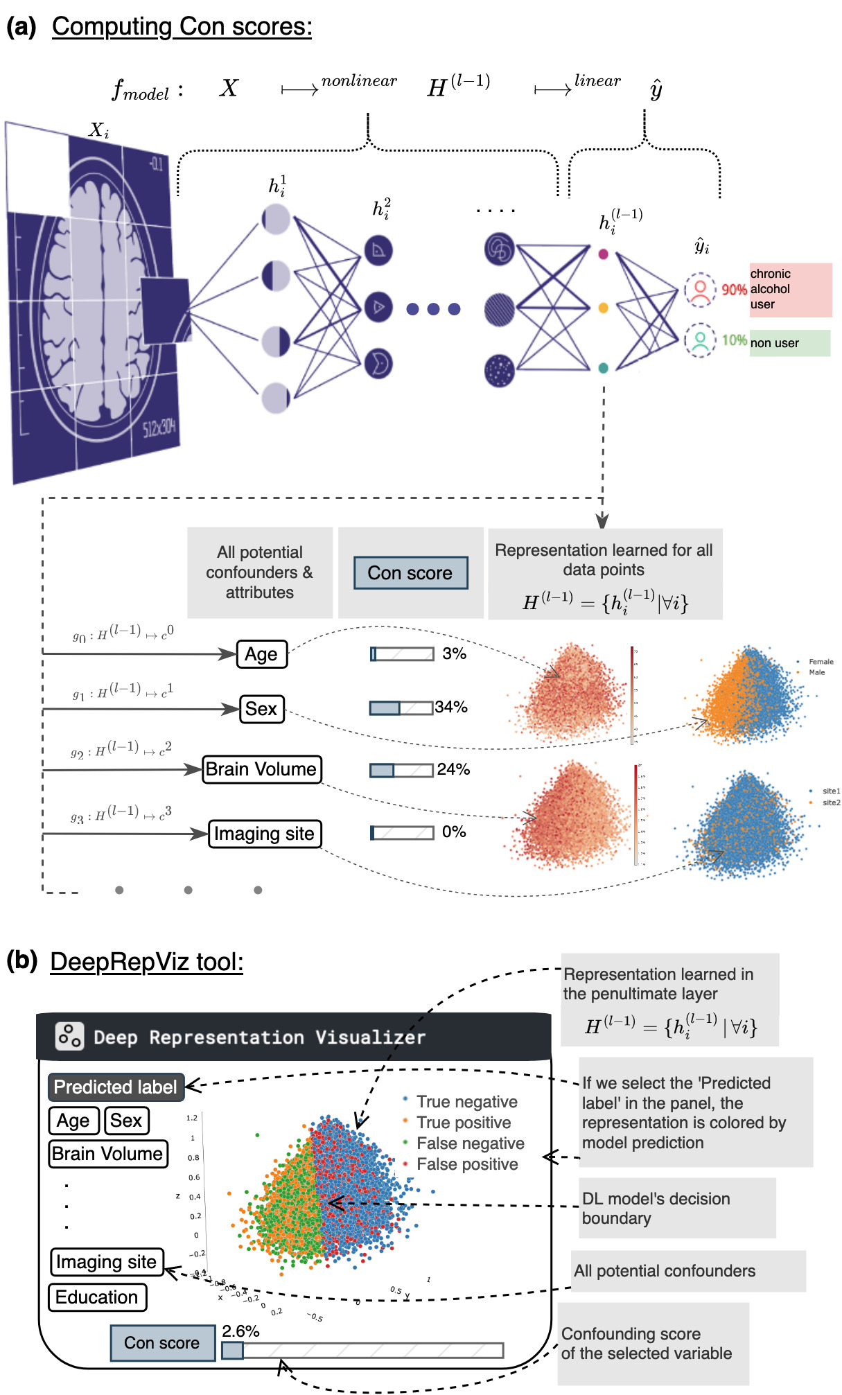
Figure 1: A demonstration of DeepRepViz and the Con-score metric: Figure (a) shows a DL model that distinguishes chronic alcohol users from non users using the participants’ structural MRI data. Con-score is computed for all relevant variables in the data from the representation learned by the DL model in its penultimate layer $H^{(l-1)}$. Con-score is highest for ‘sex’. Figure (b) shows the DeepRepViz tool and how it can be used to inspect the learned representation $H^{(l-1)}$. When we select the predicted label $\hat{y}$ in the tool, we can see the linear decision boundary of the model in $H^{(l-1)}$. This decision boundary aligns highly with the representation of sex in $H^{(l-1)}$ as shown in (a). This is also reflected in the Con-score. This implies that the model could be using the information about the participant’s sex encoded in the MRI data as a proxy to predict their alcohol use.

Results

The results on the simulated dataset show that as we systematically change the similarity between a confounder and the label, the Con-score changes proportionately, as expected. Experiments on the neuroimaging dataset reveal different potential confounders affecting the three DL model prediction tasks and provide a quantitative measure of the confounder effects. Figure 2 displays the results from both datasets.

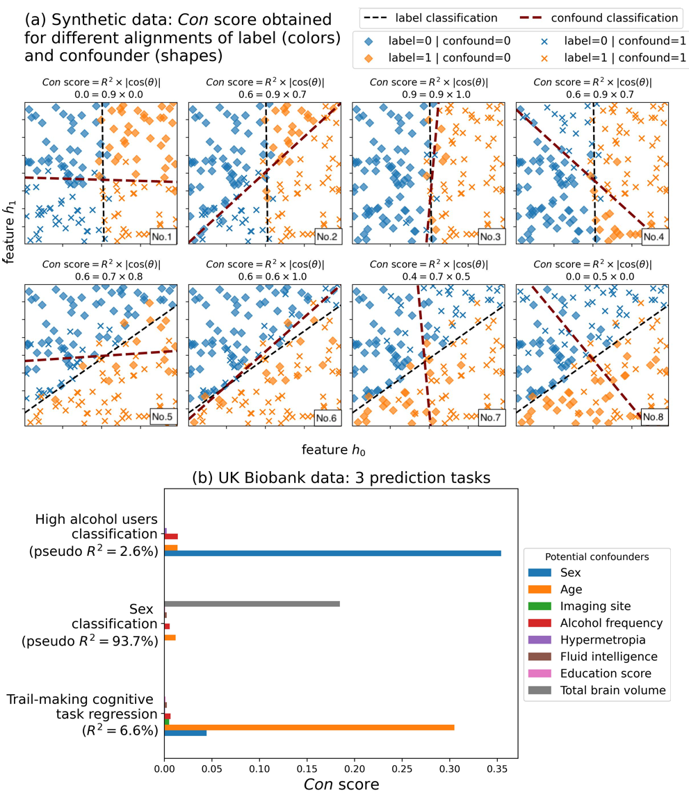
Figure 2: Results of applying Con-score metric to (a) simulated dataset and (b) UK Biobank neuroimaging dataset: (a) shows Con-scores obtained on a simulated binary classification task for 8 different levels of correlations between a confounder $c$, a binary label $y$, and the input features $H=\{h_{0},h_{1}\}$. (b) shows the Con-scores obtained for eight potential confounder variables (see legend) in three brain-phenotype prediction tasks on the UK Biobank dataset.

Results on the simulated data: In Figure 2 (a) shows the eight instances of the simulated dataset generated with different settings of the confounder $c$, a binary label $y$, and the input features $H=\{h_{0},h_{1}\}$ and the corresponding Con-score obtained for each of these cases. We can observe that the Con-scores are highest when the label classification boundary (black line) and the confound classification boundary (red line) align. In the top row, this is in instance 3 and in the bottom row, this occurs in instance 6. In these instances, $c$ is highly correlated with the label $y$. The second term in the Con-score metric, $\cos(\theta)$, captures this correlation as seen in each instance’s title in Figure 2 (a). It is easier to linearly predict $c$ in dataset instances on the top row (numbers 1 to 4) compared to the bottom row. The $R^{2}$ term of the Con-score captures this variation, as shown in each instance’s titles in Figure 2 (a). This can be observed for example, by comparing the $R^{2}$ of instance 3 with 6 or instance 1 with 8. In summary, the Con-scores are highest in the dataset instances where the correlation between $c$ and $y$ is high and $c$ is encoded in the exposure $H$. For all other cases, the Con-score drops down proportionately.

Results on neuroimaging data: Figure 2 (b) shows the results obtained for the three brain-phenotype prediction tasks. For all the tasks, the Con-score is computed for eight variables from the UK Biobank datasets as listed in the figure legend. When classifying high alcohol users, the DL model only achieves pseudo-$R^{2}=2.6\%$ and the Con-score is highest for the sex variable ($0.35$). When we visualize the representation $H^{(l-1)}$ on DeepRepViz (refer to Figure 1), we find that the majority of the participants predicted as high alcohol users by the DL model are men. This reveals that the model is picking up on the sex bias present in the data. For the cognitive performance prediction task, the DL model also achieves a low $R^{2}=6.6\%$ and the Con-score is highest for age ($0.3$). This suggests that the model tends to predict older participants as taking longer to complete the trail-making cognitive test. Visualization on the DeepRepViz tool also confirms that age is encoded in the latent representation and is aligned with the model’s prediction of the label. Interestingly, hypermetropia or long-sightedness was not a confounder for this task, although one can expect that good eyesight is important for such visual cognitive tests. For sex prediction, the Con-scores reveal that information related to the ‘total brain volume’ of the participants is encoded in the final learned representation layer (Con-score $=0.18$) but none of the other 7 variables are encoded. Whether total brain volume should be considered as a confounder or an explanation depends on the research question behind predicting sex from the brain MRI data. Nevertheless, using DeepRepViz here provided us additional insight into the DL model decisions in terms of human relatable ‘concepts’ [11] such as total brain volume.

Discussion and conclusion

Confounders cause a major nuisance when using predictive modeling methods such as DL for population neuroscience research. As the sample size of observational neuroimaging datasets grows, the problem with confounders will only worsen [9]. We propose a tool called ‘DeepRepViz’ as a solution. ‘DeepRepViz’ can be used to detect confounders in DL model predictions by inspecting the latent representation learned by the DL model in its last layer. The DeepRepViz framework consists of two components. Firstly, it includes a web-based latent representation visualization tool that can be used to qualitatively inspect the final latent representation of the DL model. Secondly, it consists of a metric called ‘Con-score’ that measures how much information related to a potential confounder is learned by the DL model in its latent representation.

Using the DeepRepViz framework in combination with predictive DL models delivers several benefits for the researchers. Firstly, the DeepRepViz framework allows researchers to compare several variables and quantify their influence on the representation learned by their DL model. Thus, it enables researchers to understand their model decisions [18] in terms of many human-understandable ‘concepts’ [11]. For example, in one of our experiments, DeepRepViz revealed that the total brain volume is an important feature for the DL model predicting sex from brain MRI. This is particularly valuable for population neuroscience studies using DL since psychological phenotypes cooccur with several extraneous demographic, socioeconomic, and environmental factors [18]. Secondly, once potential confounders are identified, researchers can test different deconfounding methods using the DeepRepViz framework. We would expect that a successful deconfounding method would reduce the Con-score to become close to 0 [19]. Finally, the tool enables researchers to not only qualitatively inspect the latent representation for signs of confounders but also look for errors arising from incorrect model configuration and optimization (refer to the tool documentation for more details).

Overall, we would emphasize that researchers should not consider identifying confounders and applying deconfounding methods as a single step of their predictive modeling analysis. Instead, they should consider confounder identification and deconfounding as an iterative procedure. Such an iterative procedure is essential for uncovering clinically relevant brain-phenotype relationships using machine learning [18]. We present DeepRepViz as a versatile tool for iterative analysis, opening pathways for medical discovery from neuroimaging data with DL. Researchers can apply DeepRepViz not only to neuroimaging but also to any predictive DL model-based discovery. It is made publicly available at https://deep-rep-viz.vercel.app and instructions on how to use the tool is provided in the tool documentation 3.

References

- [1] Samaneh Abbasi-Sureshjani et al. “Risk of training diagnostic algorithms on data with demographic bias” In Interpretable and Annotation-Efficient Learning for Medical Image Computing Springer, 2020, pp. 183–192
- [2] Yoshua Bengio, Aaron Courville and Pascal Vincent “Representation learning: A review and new perspectives” In IEEE transactions on pattern analysis and machine intelligence 35.8 IEEE, 2013, pp. 1798–1828
- [3] Richard J Chen et al. “Algorithmic fairness in artificial intelligence for medicine and healthcare” In Nature Biomedical Engineering 7.6 Nature Publishing Group UK London, 2023, pp. 719–742
- [4] Fabian Eitel et al. “Promises and pitfalls of deep neural networks in neuroimaging-based psychiatric research” In Experimental Neurology 339 Elsevier, 2021, pp. 113608
- [5] Ben Glocker, Charles Jones, Melanie Bernhardt and Stefan Winzeck “Algorithmic encoding of protected characteristics in image-based models for disease detection” In arXiv preprint arXiv:2110.14755, 2021
- [6] Ian Goodfellow, Yoshua Bengio and Aaron Courville “Deep Learning” http://www.deeplearningbook.org MIT Press, 2016
- [7] Kai Görgen, Martin N Hebart, Carsten Allefeld and John-Dylan Haynes “The same analysis approach: Practical protection against the pitfalls of novel neuroimaging analysis methods” In Neuroimage 180 Elsevier, 2018, pp. 19–30
- [8] Xue Hua et al. “Sex and age differences in atrophic rates: an ADNI study with n= 1368 MRI scans” In Neurobiology of aging 31.8 Elsevier, 2010, pp. 1463–1480
- [9] Courtland S Hyatt et al. “The quandary of covarying: A brief review and empirical examination of covariate use in structural neuroimaging studies on psychological variables” In NeuroImage 205, 2020, pp. 116225 DOI: https://doi.org/10.1016/j.neuroimage.2019.116225
- [10] M Khojaste-Sarakhsi, Seyedhamidreza Shahabi Haghighi, SMT Fatemi Ghomi and Elena Marchiori “Deep learning for Alzheimer’s disease diagnosis: A survey” In Artificial Intelligence in Medicine 130 Elsevier, 2022, pp. 102332
- [11] Been Kim et al. “Interpretability beyond feature attribution: Quantitative testing with concept activation vectors (tcav)” In International conference on machine learning, 2018, pp. 2668–2677 PMLR
- [12] Vera Komeyer et al. “The Confound Continuum: A 2D confounder assessment for AI in precision medicine”, 2023
- [13] Richard D McKelvey and William Zavoina “A statistical model for the analysis of ordinal level dependent variables” In Journal of mathematical sociology 4.1 Taylor & Francis, 1975, pp. 103–120
- [14] Nico JD Nagelkerke “A note on a general definition of the coefficient of determination” In Biometrika 78.3 Citeseer, 1991, pp. 691–692
- [15] Tomáš Paus “Population neuroscience: why and how” In Human brain mapping 31.6 Wiley Online Library, 2010, pp. 891–903
- [16] Sebastian Pölsterl, Christian Wachinger, Alzheimer’s Disease Neuroimaging Initiative and Japanese Alzheimer’s Disease Neuroimaging Initiative “Identification of causal effects of neuroanatomy on cognitive decline requires modeling unobserved confounders” In Alzheimer’s & Dementia 19.5 Wiley Online Library, 2023, pp. 1994–2005
- [17] Roshan Prakash Rane, Andreas Heinz and Kerstin Ritter “AIM in Alcohol and Drug Dependence” In Artificial Intelligence in Medicine Springer, 2022, pp. 1619–1628
- [18] Roshan Prakash Rane et al. “Eating-related variables partially explain the prospective prediction of binge drinking from structural brain features” PsyArXiv, 2023
- [19] Roshan Prakash Rane et al. “Structural differences in adolescent brains can predict alcohol misuse” In Elife 11 eLife Sciences Publications Limited, 2022, pp. e77545
- [20] Anil Rao, Joao M Monteiro, Janaina Mourao-Miranda and Alzheimer’s Disease Initiative “Predictive modelling using neuroimaging data in the presence of confounds” In Neuroimage 150 Elsevier, 2017, pp. 23–49
- [21] Ralph M Reitan “Validity of the Trail Making Test as an indicator of organic brain damage” In Perceptual and motor skills 8.3 SAGE Publications Sage CA: Los Angeles, CA, 1958, pp. 271–276
- [22] Laleh Seyyed-Kalantari et al. “Underdiagnosis bias of artificial intelligence algorithms applied to chest radiographs in under-served patient populations” In Nature medicine 27.12 Nature Publishing Group, 2021, pp. 2176–2182
- [23] Lukas Snoek, Steven Miletić and H Steven Scholte “How to control for confounds in decoding analyses of neuroimaging data” In NeuroImage 184 Elsevier, 2019, pp. 741–760
- [24] Tamas Spisak “Statistical quantification of confounding bias in machine learning models” In GigaScience 11 Oxford Academic, 2022
- [25] Cathie Sudlow et al. “UK biobank: an open access resource for identifying the causes of a wide range of complex diseases of middle and old age” In PLoS medicine 12.3 Public Library of Science, 2015, pp. e1001779
- [26] Elina Thibeau-Sutre et al. “MRI field strength predicts Alzheimer’s disease: a case example of bias in the ADNI data set” In 2022 IEEE 19th International Symposium on Biomedical Imaging (ISBI), 2022, pp. 1–4 IEEE
- [27] Sandra Vieira, Walter HL Pinaya and Andrea Mechelli “Using deep learning to investigate the neuroimaging correlates of psychiatric and neurological disorders: Methods and applications” In Neuroscience & Biobehavioral Reviews 74 Elsevier, 2017, pp. 58–75
- [28] Hon Wah Yeung et al. “Predicting sex, age, general cognition and mental health with machine learning on brain structural connectomes” In Human Brain Mapping 44.5 Wiley Online Library, 2023, pp. 1913–1933
Acknowledgements and Funding
This work was funded by the DeSBi Research Unit (DFG; KI-FOR 5363; Project ID 459422098), the consortium SFB/TRR 265 Losing and Regaining Control over Drug Intake (DFG; Project ID 402170461), FONDA (DFG; SFB 1404; Project ID: 414984028) and FOR 5187 (DFG; Project ID: 442075332).