Residual Scheduling: A New Reinforcement Learning Approach to Solving Job Shop Scheduling Problem

Abstract

Job-shop scheduling problem (JSP) is a mathematical optimization problem widely used in industries like manufacturing, and flexible JSP (FJSP) is also a common variant. Since they are NP-hard, it is intractable to find the optimal solution for all cases within reasonable times. Thus, it becomes important to develop efficient heuristics to solve JSP/FJSP. A kind of method of solving scheduling problems is construction heuristics, which constructs scheduling solutions via heuristics. Recently, many methods for construction heuristics leverage deep reinforcement learning (DRL) with graph neural networks (GNN). In this paper, we propose a new approach, named residual scheduling, to solving JSP/FJSP. In this new approach, we remove irrelevant machines and jobs such as those finished, such that the states include the remaining (or relevant) machines and jobs only. Our experiments show that our approach reaches state-of-the-art (SOTA) among all known construction heuristics on most well-known open JSP and FJSP benchmarks. In addition, we also observe that even though our model is trained for scheduling problems of smaller sizes, our method still performs well for scheduling problems of large sizes. Interestingly in our experiments, our approach even reaches zero makespan gap for 49 among 50 JSP instances whose job numbers are more than 150 on 20 machines.

1 Introduction

The job-shop scheduling problem (JSP) is a combinatorial optimization (CO) problem widely used in many industries, like manufacturing (Zhang et al., 2020; Waschneck et al., 2016). For example, a semiconductor manufacturing process can be viewed as a complex JSP problem (Waschneck et al., 2016), where a set of given jobs are assigned to a set of machines under some constraints to achieve some expected goals such as minimizing makespan which is focused on in this paper. While there are many variants of JSP (Abdolrazzagh-Nezhad and Abdullah, 2017), we also consider an extension called flexible JSP (FJSP) where job operations can be done on designated machines.

A generic approach to solving CO problems is to use mathematical programming, such as mixed integer linear programming (MILP), or constraint programming (CP). Two popular generic CO solvers for solving CO are OR-Tools (Perron and Furnon, 2019) and IBM ILOG CPLEX Optimizer (abbr. CPLEX) (Cplex, 2009). However, both JSP and FJSP, as well as many other CO problems, have been shown to be NP-hard (Garey and Johnson, 1979; Lageweg et al., 1977). That said, it is unrealistic and intractable to find the optimal solution for all cases within reasonable times. These tools can obtain the optimal solutions if sufficient time (or unlimited time) is given; otherwise, return best-effort solutions during the limited time, which usually have gaps to the optimum. When problems are scaled up, the gaps usually grow significantly.

In practice, some heuristics (Gupta and Sivakumar, 2006; Haupt, 1989) or approximate methods (Jansen et al., 2000) were used to cope with the issue of intractability. A simple greedy approach is to use the heuristics following the so-called priority dispatching rule (PDR) (Haupt, 1989) to construct solutions. These can also be viewed as a kind of solution construction heuristics or construction heuristics. Some of PDR examples are First In First Out (FIFO), Shortest Processing Time (SPT), Most WorK Remaining (MWKR), and Most Operation Remaining (MOR). Although these heuristics are usually computationally fast, it is hard to design generally effective rules to minimize the gap to the optimum, and the derived results are usually far from the optimum.

Furthermore, a generic approach to search within a search space of problem solutions is called metaheuristics, such as tabu search , genetic algorithm (GA) (Pezzella et al., 2008; Ren and Wang, 2012), and PSO algorithms (Lian et al., 2006; Liu et al., 2011). However, metaheuristics still take a high computation time, and it is not ensured to obtain the optimal solution either.

Recently, deep reinforcement learning (DRL) has made several significant successes for some applications, such as AlphaGo (Silver et al., 2016), AlphaStar (Vinyals et al., 2019), AlphaTensor (Fawzi et al., 2022), and thus it also attracted much attention in the CO problems, including chip design (Mirhoseini et al., 2021) and scheduling problems (Zhang et al., 2023). In the past, several researchers used DRL methods as construction heuristics, and their methods did improve scheduling performance, illustrated as follows. Park et al. (2020) proposed a method based on DQN (Mnih et al., 2015) for JSP in semiconductor manufacturing and showed that their DQN model outperformed GA in terms of both scheduling performance (namely gap to the optimum on makespan) and computation time. Lin et al. (2019) and Luo (2020) proposed different DQN models to decide the scheduling action among the heuristic rules and improved the makespan and the tardiness over PDRs, respectively.

A recent DRL-based approach to solving JSP/FJSP problems is to leverage graph neural networks (GNN) to design a size-agnostic representation (Zhang et al., 2020; Park et al., 2021b, a; Song et al., 2023). In this approach, graph representation has better generalization ability in larger instances and provides a holistic view of scheduling states. Zhang et al. (2020) proposed a DRL method with disjunctive graph representation for JSP, called L2D (Learning to Dispatch), and used GNN to encode the graph for scheduling decision. Besides, Song et al. (2023) extended their methods to FJSP. Park et al. (2021b) used a similar strategy of (Zhang et al., 2020) but with different state features and model structure. Park et al. (2021a) proposed a new approach to solving JSP, called ScheduleNet, by using a different graph representation and a DRL model with the graph attention for scheduling decision. Most of the experiments above showed that their models trained from small instances still worked reasonably well for large test instances, and generally better than PDRs. Among these methods, ScheduleNet achieved state-of-the-art (SOTA) performance. There are still other DRL-based approaches to solving JSP/FJSP problems, but not construction heuristics. Zhang et al. (2022) proposes another approach, called Learning to Search (L2S), a kind of search-based heuristics.

In this paper, we propose a new approach to solving JSP/FJSP, a kind of construction heuristics, also based on GNN. In this new approach, we remove irrelevant machines and jobs, such as those finished, such that the states include the remaining machines and jobs only. This approach is named residual scheduling in this paper to indicate to work on the remaining graph.

Without irrelevant information, our experiments show that our approach reaches SOTA by outperforming the above mentioned construction methods on some well-known open benchmarks, seven for JSP and two for FJSP, as described in Section 4. We also observe that even though our model is trained for scheduling problems of smaller sizes, our method still performs well for scheduling problems of large sizes. Interestingly in our experiments, our approach even reaches zero makespan gap for 49 among 50 JSP instances whose job numbers are more than 150 on 20 machines.

2 Problem Formulation

2.1 JSP and FJSP

A $n\times m$ JSP instance contains $n$ jobs and $m$ machines. Each job $J_{j}$ consists of a sequence of $k_{j}$ operations $\{O_{j,1},\dots,O_{j,k_{j}}\}$, where operation $O_{j,i}$ must be started after $O_{j,i-1}$ is finished. One machine can process at most one operation at a time, and preemption is not allowed upon processing operations. In JSP, one operation $O_{j,i}$ is allowed to be processed on one designated machine, denoted by $M_{j,i}$, with a processing time, denoted by $T^{(op)}_{j,i}$. Table 1 (a) illustrates a $3\times 3$ JSP instance, where the three jobs have 3, 3, 2 operations respectively, each of which is designated to be processed on one of the three machines $\{M_{1},M_{2},M_{3}\}$ in the table. A solution of a JSP instance is to dispatch all operations $O_{j,i}$ to the corresponding machine $M_{j,i}$ at time $\tau^{(s)}_{j,i}$, such that the above constraints are satisfied. Two solutions of the above 3x3 JSP instance are given in Figure 1 (a) and (b).

Table 1: JSP and FJSP instances

Job	Operation	$M_{1}$	$M_{2}$	$M_{3}$
Job 1	$O_{1,1}$	3
	$O_{1,2}$			5
	$O_{1,3}$		4
Job 2	$O_{2,1}$			2
	$O_{2,2}$		4
	$O_{2,3}$	3
Job 3	$O_{3,1}$	3
	$O_{3,2}$			2

(a) A $3\times 3$ JSP instance

Job	Operation	$M_{1}$	$M_{2}$	$M_{3}$
Job 1	$O_{1,1}$	3	2
	$O_{1,2}$	3		5
	$O_{1,3}$		4	3
Job 2	$O_{2,1}$			2
	$O_{2,2}$		4
	$O_{2,3}$	3
Job 3	$O_{3,1}$	3	4
	$O_{3,2}$	2		2

(b) A $3\times 3$ FJSP instance

Figure 1: Both (a) and (b) are solutions of the 3x3 JSP instance in Table 1 (a), and the former has the minimal makespan, 12. Both (c) and (d) are solutions of the 3x3 FJSP instance in Table 1 (b), and the former has the minimal makespan, 9.

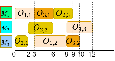
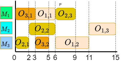
While there are different expected goals, such as makespan, tardiness, etc., this paper focuses on makespan. Let the first operation start at time $\tau=0$ in a JSP solution initially. The makespan of the solution is defined to be $T^{(mksp)}=\max(\tau^{(c)}_{j,i})$ for all operations $O_{j,i}$, where $\tau^{(c)}_{j,i}=\tau^{(s)}_{j,i}+T^{(op)}_{j,i}$ denotes the completion time of $O_{j,i}$. The makespans for the two solutions illustrated in Figure 1 (a) and (b) are 12 and 15 respectively. The objective is to derive a solution that minimizes the makespan $T^{(mksp)}$, and the solution of Figure 1 (a) reaches the optimal.

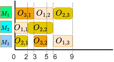
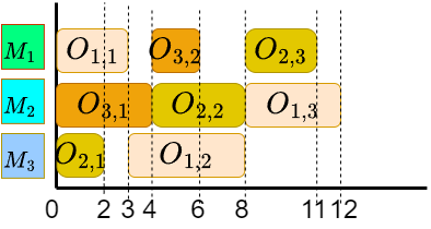
A $n\times m$ FJSP instance is also a $n\times m$ JSP instance with the following difference. In FJSP, all operations $O_{j,i}$ are allowed to be dispatched to multiple designated machines with designated processing times. Table 1 (b) illustrates a $3\times 3$ FJSP instance, where multiple machines can be designated to be processed for one operation. Figure 1 (c) illustrates a solution of an FJSP instance, which takes a shorter time than that in Figure 1 (d).

2.2 Construction Heuristics

An approach to solving these scheduling problems is to construct solutions step by step in a greedy manner, and the heuristics based on this approach is called construction heuristics in this paper. In the approach of construction heuristics, a scheduling solution is constructed through a sequence of partial solutions in a chronicle order of dispatching operations step by step, defined as follows. The $t$-th partial solution $S_{t}$ associates with a dispatching time $\tau_{t}$ and includes a partial set of operations that have been dispatched by $\tau_{t}$ (inclusive) while satisfying the above JSP constraints, and all the remaining operations must be dispatched after $\tau_{t}$ (inclusive). The whole construction starts with $S_{0}$ where none of operations have been dispatched and the dispatching time is $\tau_{0}=0$. For each $S_{t}$, a set of operations to be chosen for dispatching form a set of pairs of ($M$, $O$), called candidates $C_{t}$, where operations $O$ are allowed to be dispatched on machines $M$ at $\tau_{t}$. An agent (or a heuristic algorithm) chooses one from candidates $C_{t}$ for dispatching, and transits the partial solution to the next $S_{t+1}$. If there exists no operations for dispatching, the whole solution construction process is done and the partial solution is a solution, since no further operations are to be dispatched.

(a) $S_{0}$

(b) $S_{1}$

(c) $S_{2}$

(d) $S_{3}$

(e) $S_{4}$

(f) $S_{5}$

(g) $S_{6}$

(h) $S_{7}$

(i) $S_{8}$

Figure 2: Solution construction, a sequence of partial solutions from $S_{0}$ to $S_{8}$.

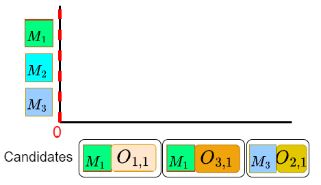
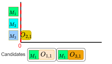
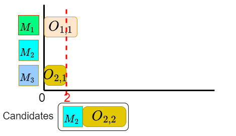
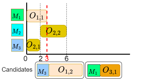
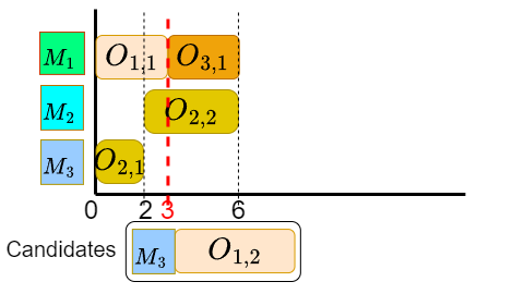
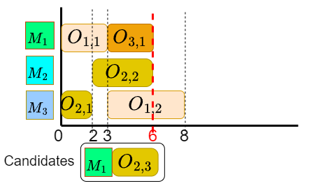
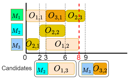
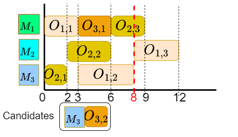
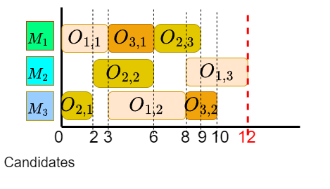
Figure 2 illustrates a solution construction process for the 3x3 JSP instance in Table 2(a), constructed through nine partial solutions step by step. The initial partial solution $S_{0}$ starts without any operations dispatched as in Figure 2 (a). The initial candidates $C_{0}$ are $\{(M_{1},O_{1,1}),(M_{3},O_{2,1}),(M_{1},O_{3,1})\}$. Following some heuristic, construct a solution from partial solution $S_{0}$ to $S_{9}$ step by step as in the Figure, where the dashed line in red indicate the time $\tau_{t}$. The last one $S_{9}$, the same as the one in Figure 1 (a), is a solution, since all operations have been dispatched, and the last operation ends at time 12, the makespan of the solution.

For FJSP, the process of solution construction is almost the same except for that one operation have multiple choices from candidates. Besides, an approach based on solution construction can be also viewed as the so-called Markov decision process (MDP), and the MDP formulation for solution construction is described in more detail in the appendix.

3 Our Approach

In this section, we present a new approach, called residual scheduling, to solving scheduling problems. We introduce the residual scheduling in Subsection 3.1, describe the design of the graph representation in Subsection 3.2, propose a model architecture based on graph neural network in Subsection 3.3 and present a method to train this model in Subsection 3.4;

3.1 Residual Scheduling

In our approach, the key is to remove irrelevant information, particularly for operations, from states (including partial solutions). An important benefit from this is that we do not need to include all irrelevant information while training to minimize the makespan. Let us illustrate by the state for the partial solution $S_{3}$ at time $\tau_{3}=3$ in Figure 2 (d). All processing by $\tau_{3}$ are irrelevant to the remaining scheduling. Since operations $O_{1,1}$ and $O_{2,1}$ are both finished and irrelevant the rest of scheduling, they can be removed from the state of $S_{3}$. In addition, operation $O_{2,2}$ is dispatched at time 2 (before $\tau_{3}=3$) and its processing time is $T^{(op)}_{2,1}=4$, so the operation is marked as ongoing. Thus, the operation can be modified to start at $\tau_{3}=3$ with a processing time $4-(3-2)$. Thus, the modified state for $S_{3}$ do not contain both $O_{1,1}$ and $O_{2,1}$, and modify $O_{2,2}$ as above. Let us consider two more examples. For $S_{4}$, one more operation $O_{2,2}$ is dispatched and thus marked as ongoing, however, the time $\tau_{4}$ remains unchanged and no more operations are removed. In this case, the state is almost the same except for including one more ongoing operation $O_{2,2}$. Then, for $S_{5}$, two more operations $O_{3,1}$ and $O_{2,2}$ are removed and the ongoing operation $O_{1,2}$ changes its processing time to the remaining time (5-3).

For residual scheduling, we also reset the dispatching time $\tau=0$ for all states with partial solutions modified as above, so we derive makespans which is also irrelevant to the earlier operations. Given a scheduling policy $\pi$, $T^{(mksp)}_{\pi}(S)$ is defined to be the makespan derived from an episode starting from states $S$ by following $\pi$, and $T^{(mksp)}_{\pi}(S,a)$ the makespan by taking action $a$ on $S$.

3.2 Residual Graph Representation

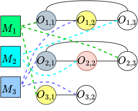
In this paper, our model design is based on graph neural network (GNN), and leverage GNN to extract the scheduling decision from the relationship in graph. In this subsection, we present the graph representation. Like many other researchers such as Park et al. (2021a), we formulate a partial solution into a graph $\mathcal{G}=(\mathcal{V},\mathcal{E})$, where $\mathcal{V}$ is a set of nodes and $\mathcal{E}$ is a set of edges. A node is either a machine node $M$ or an operation node $O$. An edge connects two nodes to represent the relationship between two nodes, basically including three kinds of edges, namely operation-to-operation ($O\to O$), machine-to-operation ($M\to O$) and operation-to-machine ($O\to M$). All operations in the same job are fully connected as $O\to O$ edges. If an operation $O$ is able to be performed on a machine $M$, there exists both $O\to M$ and $M\to O$ directed edges. In (Park et al., 2021a), they also let all machines be fully connected as $M\to M$ edges. However, our experiments in section 4 show that mutual $M\to M$ edges do not help much based on our Residual Scheduling. An illustration for graph representation of $S_{3}$ is depicted in Figure 3 (a).

(a) Graph for $S_{3}$

(b) Graph embedding

(c) Score function

Figure 3: Graph representation and networks.

In the graph representation, all nodes need to include some attributes so that a partial solution $S$ at the dispatching time $\tau$ can be supported in the MDP formulation (in the appendix). Note that many of the attributes below are normalized to reduce variance. For nodes corresponding to operations $O_{j,i}$, we have the following attributes:

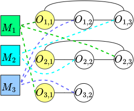
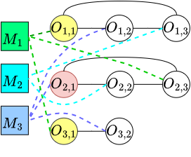
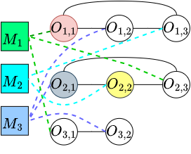
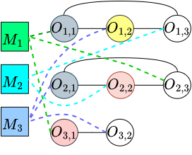
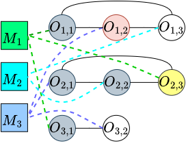
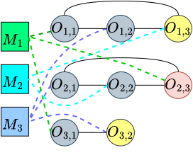
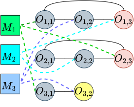
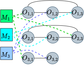
Status $\phi_{j,i}$: The operation status $\phi_{j,i}$ is completed if the operation has been finished by $\tau$, ongoing if the operation is ongoing (i.e., has been dispatched to some machine by $\tau$ and is still being processed at $\tau$), ready if the operation designated to the machine which is idle has not been dispatched yet and its precedent operation has been finished, and unready otherwise. For example, in Figure 3 (a), the gray nodes are completed, the red ongoing, the yellow ready and the white unready. In our residual scheduling, there exists no completed operations in all partial solutions, since they are removes for irrelevance of the rest of scheduling. The attribute is a one-hot vector to represent the current status of the operation, which is one of ongoing, ready and unready. Illustration for all states $S_{0}$ to $S_{8}$ are shown in the appendix.

Normalized processing time $\bar{T}^{(op)}_{j,i}$: Let the maximal processing time be $T^{(op)}_{max}=\max_{\forall j,i}(T^{(op)}_{j,i})$. Then, $\bar{T}^{(op)}_{j,i}=T^{(op)}_{j,i}/T^{(op)}_{max}$. In our residual scheduling, the operations that have been finished are removed in partial solutions and therefore their processing time can be ignored; the operations that has not been dispatched yet still keep their processing times the same; the operations that are ongoing change their processing times to the remaining times after the dispatching time $\tau_{t}$. As for FJSP, the operations that has not been dispatched yet may have several processing times on different machines, and thus we can simply choose the average of these processing times.

Normalized job remaining time $\bar{T}^{(job)}_{j,i}$: Let the rest of processing time for job $J_{j}$ be $T^{(job)}_{j,i}=\sum_{\forall i^{\prime}\geq i}T^{(op)}_{j,i^{\prime}}$, and let the processing time for the whole job $j$ be $T^{(job)}_{j}=\sum_{\forall i^{\prime}}T^{(op)}_{j,i^{\prime}}$. In practice, $T^{(job)}_{j}$ is replaced by the processing time for the original job $j$. Thus, $\bar{T}^{(job)}_{j,i}=T^{(job)}_{j,i}/T^{(job)}_{j}$. For FJSP, since operations $O_{j,i}$ can be dispatched to different designated machines $M_{l}$, say with the processing time $T^{(op)}_{j,i,l}$, we simply let $T^{(op)}_{j,i}$ be the average of $T^{(op)}_{j,i,l}$ for all $M_{l}$.

For machine nodes corresponding to machines $M_{l}$, we have the following attributes:

Machine status $\phi_{l}$: The machine status $\phi_{l}$ is processing if some operation has been dispatched to and is being processed by $M_{l}$ at $\tau$, and idle otherwise (no operation is being processed at $\tau$). The attribute is a one-hot vector to represent the current status, which is one of processing and idle.

Normalized operation processing time $\bar{T}^{(mac)}_{l}$: On the machine $M_{l}$, the processing time $T^{(mac)}_{l}$ is $T^{(op)}_{j,i}$ (the same as the normalized processing time for node $O_{j,i}$) if the machine status is processing, i.e., some ongoing operation $O_{j,i}$ is being processed but not finished yet, is zero if the machine status is idle. Then, this attribute is normalized to $T^{(op)}_{max}$ and thus $\bar{T}^{(mac)}_{l}=T^{(mac)}_{l}/T^{(op)}_{max}$.

Now, consider edges in a residual scheduling graph. As described above, there exists three relationship sets for edges, $O\to O$, $O\to M$ and $M\to O$. First, for the same job, say $J_{j}$, all of its operation nodes for $O_{j,i}$ are fully connected. Note that for residual scheduling the operations finished by the dispatching time $\tau$ are removed and thus have no edges to them. Second, a machine node for $M_{l}$ is connected to an operation node for $O_{j,i}$, if the operation $O_{j,i}$ is designated to be processed on the machine $M_{l}$, which forms two edges $O\to M$ and $M\to O$. Both contains the following attribute.

Normalized operation processing time $\bar{T}^{(edge)}_{j,i,l}$: The attribute is $\bar{T}^{(edge)}_{j,i,l}=T^{(op)}_{j,i}/T^{(op)}_{max}$. Here, $T^{(op)}_{j,i}=T^{(op)}_{j,i,l}$ in the case of FJSP. If operation $O_{j,i}$ is ongoing (or being processed), $T^{(op)}_{j,i}$ is the remaining time as described above.

3.3 Graph Neural Network

In this subsection, we present our model based on graph neural network (GNN). GNN are a family of deep neural networks (Battaglia et al., 2018) that can learn representation of graph-structured data, widely used in many applications (Lv et al., 2021; Zhou et al., 2020). A GNN aggregates information from node itself and its neighboring nodes and then update the data itself, which allows the GNN to capture the complex relationships within the data graph. For GNN, we choose Graph Isomorphism Network (GIN), which was shown to have strong discriminative power (Xu et al., 2019) and summarily reviewed as follows. Given a graph $\mathcal{G}=(\mathcal{V},\mathcal{E})$ and $K$ GNN layers ($K$ iterations), GIN performs the $k$-th iterations of updating feature embedding $h^{(k)}$ for each node $v\in\mathcal{V}$:

$$h^{(k)}_{v}=MLP^{(k)}((1+\epsilon^{(k)})h^{(k-1)}_{v}+\sum_{u\in N_{b}(v)}h^{(k-1)}_{u}),$$ (1)

where $h^{(k)}_{v}$ is the embedding of node $v$ at the $k$-th layer, $\epsilon^{(k)}$ is an arbitrary number that can be learned, and $N_{b}(v)$ is the neighbors of $v$ via edges in $\mathcal{E}$. Note that $h^{(0)}_{v}$ refers to its raw features for input. $MLP^{(k)}$ is a Multi-Layer Perceptron (MLP) for the $k$-th layer with a batch normalization (Ioffe and Szegedy, 2015).

Furthermore, we actually use heterogeneous GIN, also called HGIN, since there are two types of nodes, machine and operation nodes, and three relations, $O\to O$, $O\to M$ and $M\to O$ in the graph representation. Although we do not have cross machine relations $M\to M$ as described above, updating machine nodes requires to include the update from itself as in (1), that is, there is also one more relation $M\to M$. Thus, HGIN encodes graph information between all relations by using the four MLPs as follows,

$$h^{(k+1)}_{v}=\sum_{\mathcal{R}}MLP^{(k+1)}_{\mathcal{R}}((1+\epsilon^{(k+1)}_{\mathcal{R}})h^{(k)}_{v}+\sum_{u\in N_{\mathcal{R}}(v)}h^{(k)}_{u})$$ (2)

where $\mathcal{R}$ is one of the above four relations and $MLP^{(k)}_{\mathcal{R}}$ is the MLP for $\mathcal{R}$. For example, for $S_{0}$ in Figure 2 (a), the embedding of $M_{1}$ in the $(k+1)$-st iteration can be derived as follows.

$$h^{(k+1)}_{M_{1}}=MLP^{(k+1)}_{MM}((1+\epsilon^{(k+1)}_{MM})h^{(k)}_{M_{1}})+MLP^{(k+1)}_{OM}((h^{(k)}_{O_{1,1}}||\bar{T}_{1,1,1})+(h^{(k)}_{O_{2,3}}||\bar{T}_{2,3,1})+(h^{(k)}_{O_{3,1}}||\bar{T}_{3,1,1}))$$ (3)

Similarly, the embedding of $O_{1,1}$ in the $(k+1)$-st iteration is:

$$h^{(k+1)}_{O_{1,1}}=MLP^{(k+1)}_{OO}((1+\epsilon^{(k+1)}_{OO})h^{(k)}_{O_{1,1}}+h^{(k)}_{O_{1,2}}+h^{(k)}_{O_{1,3}})+MLP^{(k+1)}_{MO}((h^{(k)}_{M_{1}}||\bar{T}_{1,1,1}))$$ (4)

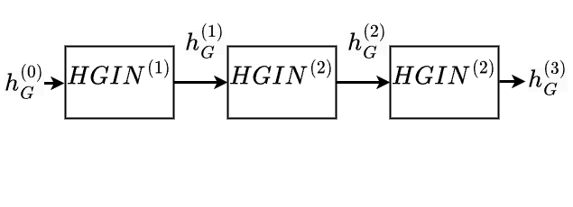
In our approach, an action includes the two phases, graph embedding phase and action selection phase. Let $h^{(k)}_{\mathcal{G}}$ denote the whole embedding of the graphs $\mathcal{G}$, including all $h^{(k)}_{O\in\mathcal{G}}$ and $h^{(k)}_{M\in\mathcal{G}}$. In the graph embedding phase, we use an HGIN to encode node and graph embeddings as described above. An example with three HGIN layers is illustrated in Figure 3 (b).

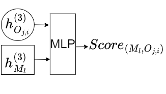
In the action selection phase, we select an action based on a policy, after node and graph embedding are encoded in the graph embedding phase. The policy is described as follows. First, collect all ready operations $O$ to be dispatched to machines $M$. Then, for all pairs ($M$, $O$), feed their node embeddings ($h^{(k)}_{M}$, $h^{(k)}_{O}$) into a MLP $Score(M,O)$ to calculate their scores as shown in Figure 3 (c). The probability of selecting ($M$, $O$) is calculated based on a softmax function of all scores, which also serves as the model policy $\pi$ for the current state.

3.4 Policy-Based RL Training

In this paper, we propose to use a policy-based RL training mechanism that follows REINFORCE (Sutton and Barto, 2018) to update our model by policy gradient with a normalized advantage makespan with respect to a baseline policy $\pi_{b}$ as follows.

$$A_{\pi}(S,a)=\frac{T^{(mksp)}_{\pi_{b}}(S,a)-T^{(mksp)}_{\pi}(S,a)}{T^{(mksp)}_{\pi_{b}}(S,a)}$$ (5)

In this paper, we choose a lightweight PDR, MWKR, as baseline $\pi_{b}$, which performed best for makespan among all PDRs reported from the previous work (Zhang et al., 2020). In fact, our experiment also shows that using MWKR is better than the other PDRs shown in the appendix. The model for policy $\pi$ is parametrized by $\theta$, which is updated by $\nabla_{\theta}log\pi_{\theta}A_{\pi_{\theta}}(S_{t},a_{t})$. Our algorithm based on REINFORCE is listed in the appendix.

4 Experiments

4.1 Experimental Settings and Evaluation Benchmarks

In our experiments, the settings of our model are described as follows. All embedding and hidden vectors in our model have a dimension of 256. The model contains three HGIN layers for graph embedding, and an MLP for the score function, as shown in Figure 3 (b) and (c). All MLP networks including those in HGIN and for score contain two hidden layers. The parameters of our model, such as MLP, generally follow the default settings in PyTorch (Paszke et al., 2019) and PyTorch Geometric (Fey and Lenssen, 2019). More settings are in the appendix.

Each of our models is trained with one million episodes, each with one scheduling instance. Each instance is generated by following the procedure which is used to generate the TA dataset (Taillard, 1993). Given ($N$, $M$), we use the procedure to generate an $n\times m$ JSP instance by conforming to the following distribution, $n\sim\mathcal{U}(3,N)$, $m\sim\mathcal{U}(3,n)$, and operation count $k_{j}=m$, where $\mathcal{U}(x,y)$ represents a distribution that uniformly samples an integer in a close interval $[x,y]$ at random. The details of designation for machines and processing times refer to (Taillard, 1993) and thus are omitted here. We choose (10,10) for all experiments, since (10,10) generally performs better than the other two as described in the appendix. Following the method described in Subsection 3.4, the model is updated from the above randomly generated instances. For testing our models for JSP and FJSP, seven JSP open benchmarks and two FJSP open benchmarks are used, as listed in the appendix.

The performance for a given policy method $\pi$ on an instance is measured by the makespan gap $G$ defined as

$$G=\frac{T^{(mksp)}_{\pi}-T^{(mksp)}_{\pi*}}{T^{(mksp)}_{\pi*}}$$ (6)

where $T^{(mksp)}_{\pi*}$ is the optimal makespan or the best-effort makespan, from a mathematical optimization tool, OR-Tools, serving as $\pi*$. By the best-effort makespan, we mean the makespan derived with a sufficiently large time limitation, namely half a day with OR-Tools. For comparison in experiments, we use a server with Intel Xeon E5-2683 CPU and a single NVIDIA GeForce GTX 1080 Ti GPU. Our method uses a CPU thread and a GPU to train and evaluate, while OR-Tools uses eight threads to find the solution.

4.2 Experiments for JSP

For JSP, we first train a model based on residual scheduling, named RS. For ablation testing, we also train a model, named RS+op, by following the same training method but without removing irrelevant operations. When using these models to solve testing instances, action selection is based on the greedy policy that simply chooses the action $(M,O)$ with the highest score deterministically, obtained from the score network as in Figure 3 (c).

For comparison, we consider the three DRL construction heuristics, respectively developed in (Zhang et al., 2020) called L2D, (Park et al., 2021b) by Park et al., and (Park et al., 2021a), called ScheduleNet. We directly use the performance results of these methods for open benchmarks from their articles. For simplicity, they are named L2D, Park and SchN respectively in this paper. We also include some construction heuristics based PDR, such as MWKR, MOR, SPT and FIFO. Besides, to derive the gaps to the optimum in all cases, OR-Tools serve as $\pi*$ as described in (6).

Now, let us analyze the performances of RS as follows. Table 2 shows the average makespan gaps for each collection of JSP TA benchmarks with sizes, 15×15, 20×15, 20×20, 30×15, 30×20, 50×15, 50×20 and 100×20, where the best performances (the smallest gaps) are marked in bold. In general, RS performs the best, and generally outperforms the other methods for all collections by large margins, except for that it has slightly higher gaps than RS+op for the two collections, 15 $\times$ 15 and 20 $\times$ 20. In fact, RS+op also generally outperforms the rest of methods, except for that it is very close to SchN for two collections. For the other six open benchmarks, ABZ, FT, ORB, YN, SWV and LA, the performances are similar and thus presented in the appendix. It is concluded that RS generally performs better than other construction heuristics by large margins.

Table 2: Average makespan gaps for TA benchmarks.

Size	15$\times$15	20$\times$15	20$\times$20	30$\times$15	30$\times$20	50$\times$15	50$\times$20	100$\times$20	$Avg.$
RS	0.148	0.165	0.169	0.144	0.177	0.067	0.100	0.026	0.125
RS+op	0.143	0.193	0.159	0.192	0.213	0.123	0.126	0.050	0.150
MWKR	0.191	0.233	0.218	0.239	0.251	0.168	0.179	0.083	0.195
MOR	0.205	0.235	0.217	0.228	0.249	0.173	0.176	0.091	0.197
SPT	0.258	0.328	0.277	0.352	0.344	0.241	0.255	0.144	0.275
FIFO	0.239	0.314	0.273	0.311	0.311	0.206	0.239	0.135	0.254
L2D	0.259	0.300	0.316	0.329	0.336	0.223	0.265	0.136	0.270
Park	0.201	0.249	0.292	0.246	0.319	0.159	0.212	0.092	0.221
SchN	0.152	0.194	0.172	0.190	0.237	0.138	0.135	0.066	0.161

4.3 Experiments for FJSP

Table 3: Average makespan gaps for FJSP open benchmarks

Method	MK	LA(rdata)	LA(edata)	LA(vdata)
RS	0.232	0.099	0.146	0.031
RS+op	0.254	0.113	0.168	0.029
DRL-G	0.254	0.111	0.150	0.040
MWKR	0.282	0.125	0.149	0.051
MOR	0.296	0.147	0.179	0.061
SPT	0.457	0.277	0.262	0.182
FIFO	0.307	0.166	0.220	0.075

For FJSP, we also train a model based on residual scheduling, named RS, and an ablation version, named RS+op, without removing irrelevant operations. We compares ours with one DRL construction heuristics developed by (Song et al., 2023), called DRL-G, and four PDR-based heuristics, MOR, MWKR, SPT and FIFO. We directly use the performance results of these methods for open datasets according to the reports from (Song et al., 2023).

Table 3 shows the average makespan gaps in the four open benchmarks, MK, LA(rdata), LA(edata) and LA(vdata). From the table, RS generally outperforms all the other methods for all benchmarks by large margins, except for that RS+op is slightly better for the benchmark LA(vdata).

5 Discussions

In this paper, we propose a new approach, called residual scheduling, to solving JSP an FJSP problems, and the experiments show that our approach reaches SOTA among DRL-based construction heuristics on the above open JSP and FJSP benchmarks. We further discusses three issues: large instances, computation times and further improvement.

Figure 4: Average makespan gaps of JSP instances with different problem sizes.

First, from the above experiments particularly for TA benchmark for JSP, we observe that the average gaps gets smaller as the number of jobs increases, even if we use the same model trained with $(N,M)=(10,10)$. In order to investigate size-agnostics, we further generate 13 collections of JSP instances of sizes for testing, from 15 $\times$ 15 to 200 $\times$ 20, and generate 10 instances for each collection by using the procedure above. Figure 4 shows the average gaps for these collections for RS and L2D, and these collections are listed in the order of sizes in the x-axis. Note that we only show the results of L2D in addition to our RS, since L2D is the only open-source among the above DRL heuristics. In Figure 4, it is observed that RS is much better than L2D. Interestingly, using RS, the average gaps are nearly zero for the collections with sizes larger than 100 $\times$ 15, namely, 100 $\times$ 15, 100 $\times$ 20, 150 $\times$ 15, 200 $\times$ 15 and 200 $\times$ 20. Among the 50 JSP instances in the five collections, 49 reaches zero makespan gaps. A strong implication is that our RS approach can be scaled up for job sizes and even reach the optimal for sufficient large job count.

Second, the computation times for RS are relatively small and has low variance like most of other construction heuristics. Here, we just use the collection of TA 100x20 for illustration. It takes about 30 seconds on average for both RS and RS+op, about 28 for L2D and about 444 for SchN. In contrast, it takes about 4000 seconds with high variance for OR-Tools. The times for other collections are listed in more detail in the appendix.

Table 4: Average makespan gaps for FJSP open benchmark.

Method	MK	LA(rdata)	LA(edata)	LA(vdata)
RS	0.232	0.099	0.146	0.031
RS+100	0.154	0.047	0.079	0.007
DRL-G	0.254	0.111	0.150	0.040
DRL+100	0.190	0.058	0.082	0.014

Third, as proposed by Song et al. (2023), construction heuristics can further improve the gap by constructing multiple solutions based on the softmax policy, in addition to the greedy policy. They had a version constructing 100 solutions for FJSP, called DRL+100 in this paper. In this paper, we also implement a RS version for FJSP based on the softmax policy, as described in Subsection 3.3, and then use the version, called RS+100, to constructing 100 solutions. In Table 4, the experimental results show that RS+100 performs the best, much better than RS, DRL-G and DRL+100. An important property for such an improvement is that constructing multiple solutions can be done in parallel. That is, for construction heuristics, the solution quality can be improved by adding more computation powers.

Appendix

In this appendix, we include the following items, described in the subsequent subsections respectively.

• Code, datsets and model weights.

• Formulation of Markov decision process for solution construction.

• Illustration of graph representation for partial solutions in Figure 2.

• REINFORCE algorithm in our approach.

• Experimental settings.

• Additional Experiments.

Appendix A Code, Datasets and Model Weights

Our code, datasets and pre-trained weights are in the supplementary folder ResidualScheduling. The code includes the following: First, setup the virtual environment, Then, install required packages in the environment. Finally, execute the code with the commands in the README file. All hyperparameters are also listed in README file.

We collect the following dataset for evaluation. For JSP dataset, we collect 13 collections generated for the experiments shown in Figure 4, and other seven JSP benchmarks, TA, ABZ, FT, ORB, YN, SWV and LA. For FJSP dataset, we collect two FJSP benchmarks, MK and LA, and the instances generated from the work (Song et al., 2023).

There are four weights according to the final models for RS and RS+op with JSP and FJSP cases, denoted as RS_JSP, RS+op_JSP, RS_FJSP, and RS+op_FJSP.

Appendix B Formulation of Markov Decision Process for Solution Construction

In Subsection 2.2, an approach based on solution construction can be also viewed as the so-called Markov decision process (MDP). An MDP is a stochastic decision-making process widely used in reinforcement learning, generally defined by a tuple $(\mathcal{S},\mathcal{A},\mathcal{R},\mathcal{P})$, where $\mathcal{S}$ is the finite set of the states, $\mathcal{A}$ is the set of the available actions, $\mathcal{R}$ is the reward function and $\mathcal{P}$ is the transition probability function. The objective is to find a policy that maximizes the agent’s cumulative rewards.

Following the above MDP definition, we formulate the process of solution construction for JSP and FJSP problems as follows.

• $\mathcal{S}$ specifies states each representing an instance associated with the information of partial solutions $S$ like those in Figure 2.

• $\mathcal{A}$ specifies actions each of which selects machine-operation pairs ($M,O$) to dispatch the operation $O$ on the machine $M$ on given states.

• $\mathcal{R}$ specifies a reward to indicate a negative of the additional processing time for the dispatched action.

• $\mathcal{P}$ specifies how states are transited from one partial solution $S$ to the next $S^{\prime}$ after an action, as described in Subsection 2.2 accordingly.

An episode starts from the initial partial solution and repeats transitions till the end when the partial solution is a solution. The cumulative reward is the negative of makespan $T^{(mksp)}$, i.e., the total complete time. The objective is to maximize the cumulative reward, i.e., minimize the makespan. In the past, many methods for JSP and FJSP based on reinforcement learning such as (Park et al., 2020; Luo, 2020; Zhang et al., 2020; Park et al., 2021b, a) followed this MDP formulation.

Appendix C Illustration of Graph Representation for Partial Solutions

In Figure 3 (a), we illustrate graph representation of $S_{3}$. In this section, Figure 5 illustrates the step-by-step graph representations respectively corresponding to all the partial solutions in Figure 2 in Subsection 3.2. Again, the gray nodes are completed, the red ongoing, the yellow ready and the white unready.

(a) $S_{0}$

(b) $S_{1}$

(c) $S_{2}$

(d) $S_{3}$

(e) $S_{4}$

(f) $S_{5}$

(g) $S_{6}$

(h) $S_{7}$

(i) $S_{8}$

Figure 5: (a)-(i) are corresponding to partial solutions in Figure 2 (a)-(i), respectively.

Appendix D REINFORCE Algorithm in Our Approach

Our residual scheduling approach basically follows REINFORCE (Sutton and Barto, 2018) to update our model by policy gradient with a normalized advantage makespan based on a baseline policy and an entropy bonus to ensure sufficient exploration like PPO. Algorithm 1 (next page) shows our REINFORCE training process with the normalized advantage makespan described in Section 3.4. The model policy $\pi_{\theta}$ is parameterized by $\theta$ initialized at random, and a baseline policy $\pi_{b}$ is given, which is a lightweight PDR, MWKR, in this paper. The learning rate $\alpha\in(0,1)$ is initialized to $10^{-4}$ and decayed by a factor of 0.99 every $P=1000$ episodes in this paper.

Algorithm 1 REINFORCE with a normalized advantage for JSP and FJSP

1:  Input: Initial policy $\pi_{\theta}$, learning rate $\alpha\in(0,1)$, entropy bonus coefficient $c$, a baseline policy $\pi_{b}$;

2:  for Episode $e=0,1,\cdots$ do

3:     Use policy $\pi_{\theta}$ to rollout an episode: $\{S_{1},a_{1},S_{2},a_{2},\cdots,S_{T}\}$

4:     for $t=0,1,2,\cdots T$ do

5:        Use the baseline policy $\pi_{b}$ to rollout and obtain $T^{(mksp)}_{\pi_{b}}(S_{t},a_{t})$

6:        Calculate $T^{(mksp)}_{\pi_{\theta}}(S_{t},a_{t})$

7:        Calculate normalized advantage $A_{\pi_{\theta}}(S_{t},a_{t})$ following Equation (5)

8:        Update policy $\theta=\theta+\alpha\nabla_{\theta}(log\pi_{\theta}A_{\pi_{\theta}}(S_{t},a_{t})+cH_{\pi_{\theta}}(S_{t}))$

9:     end for

10:     Update learning rate every $P=1000$ episodes

11:  end for

Appendix E Experimental Settings

In this section, we first describe settings of our model in Appendix E.1 and then list the details of JSP and FJSP open benchmarks used in our experiments in Appendix E.2.

E.1 Model Settings

In this subsection, we first list the settings of our model in Table 5. Particularly, the entropy bonus coefficient $c$ is used for the weight of entropy in line 8 of Algorithm 1, and the initial learning rate $\alpha$ is used in lines 1 and 8 of Algorithm 1.

Table 5: Model hyperparameters.

Item	Value	Description
HGIN layers	3	Layer number of GNN.
FC layers of MLP	2	Layer number of MLP.
Hidden dimension	256	Hidden vector dimension for GNN and policy network.
Episodes	1,000,000	Training episodes
Entropy bonus coefficient ($c$)	$10^{-2}$	The weight of entropy bonus in the loss function.
Initial learning rate ($\alpha$)	$10^{-4}$	Initialized with $10^{-4}$ and then decayed with 0.99 rate for every 1000 episodes
Optimizer	Adam	Adam with $\beta_{1}=0.9$ and $\beta_{2}=0.999$

In practice, one model is trained for each of $(N,M)$, (6,6), (10,10) and (15,15), and each of baseline policies, MWKR, MOR, SPT and FIFO. Each of models is trained with 1000 iterations, for each of which model parameters are updated with 1000 episodes (one million of episodes in total). It takes about one day to train with 200,000 episodes. For each episode, one scheduling instance is generated for training by the procedure subject to $(N,M)$ as in Subsection 4.1.

For JSP, we also generate a validation dataset of the three collections, 20 $\times$ 20, 50 $\times$ 20 and 100 $\times$ 20, each with 10 instances. Among the 1000 sets of model parameters, the one performing best for the validation dataset is chosen for testing in the rest of experiments. Table 6 shows the average makespans of the four models trained with different baselines respectively and with (10,10) on the validation dataset. The one with MWKR clearly outperforms other baselines on the validation dataset. Thus, MWKR is chosen as the baseline in this paper. Similarly, Table 7 shows the average makespans of three models trained with different training sizes (6,6), (10,10) and (15,15) respectively and with MWKR on the validation dataset. The one with (10,10) performs best, except for that the one with (15,15) performs slightly better for the collection of 100 $\times$ 20. Thus, this paper still chooses (10,10) since it performs well in general and has less training costs when compared to (15,15).

Table 6: Average makespans of models with different baseline policies $\pi_{b}$ on JSP validation dataset.

$\pi_{b}$	20$\times$20	50$\times$20	100$\times$20
MWKR	1803.1	3147.3	5676.0
MOR	1831.7	3229.8	5728.3
SPT	1813.8	3201.7	5718.7
FIFO	1826.4	3177.6	5692.9

Table 7: Average makespans of models with different $(N,M)$ on JSP validation dataset.

Method	20$\times$20	50$\times$20	100$\times$20
RS (6,6)	1822.8	3242.7	5784.4
RS (10,10)	1803.1	3147.3	5676.0
RS (15,15)	1820.7	3170.6	5670.4

For FJSP, we simply use the validation set used by (Song et al., 2023). Table 8 shows the average makespans of three models trained with different training sizes (6,6), (10,10) and (15,15) respectively and with MWKR on the validation dataset. The one with (10,10) outperforms others for all the collections in Song et al. (2023). Hence, (10,10) is also chosen in FJSP experiments in this paper.

Table 8: Average makespans of models with different $(N,M)$ on FJSP validation dataset.

Method	10 $\times$ 5	15 $\times$ 10	20 $\times$ 5	20 $\times$ 10
RS (6,6)	106.25	164.98	209.77	210.57
RS (10,10)	106.00	163.88	209.07	210.18
RS (15,15)	106.15	163.95	209.57	210.47

E.2 Open Benchmarks

Table 9 lists the information about JSP and FJSP open benchmarks used in this paper. For JSP, TA benchmark has most instances, including 8 categories, 15 $\times$ 15, 20 $\times$ 15, 20 $\times$ 20, 30 $\times$ 15, 30 $\times$ 20, 50 $\times$ 15, 50 $\times$ 20 and 100 $\times$ 20. For each category, there are 10 instances generated by their procedure. For other JSP benchmarks, they cover different problem sizes and data distributions as in the table.

For FJSP, two popular open benchmarks are MK, also known as Brandimarte instances, and LA, also known as Hurink instances (to distinguish LA benchmark for JSP). Hurink instances are categories into three types, edata, rdata and vdata, according to different distribution for assignable machines, denoted by LA(edata), LA(rdata) and LA(vdata) respectively, as described in (Hurink et al., 1994).

Table 9: Open benchmarks.

Type	Benchmark	Instances	Min size	Max size
JSP	TA (Taillard, 1993)	80	15$\times$15	100$\times$20
	ABZ (Adams et al., 1988)	5	10$\times$10	20$\times$15
	FT (Muth and Thompson, 1963)	3	6$\times$6	20$\times$5
	ORB (Applegate and Cook, 1991)	10	10$\times$10	10$\times$10
	YN (Yamada and Nakano, 1992)	4	20$\times$20	20$\times$20
	SWV (Storer et al., 1992)	20	20$\times$10	50$\times$10
	LA (Lawrence, 1984)	40	10$\times$5	30$\times$10
FJSP	MK (Brandimarte, 1993)	10	10$\times$6	20$\times$15
	LA (Hurink et al., 1994)	120	10$\times$5	30$\times$10

Appendix F Additional Experiments

This section shows additional experiments conducted to support residual scheduling as follows.

• Appendix F.1 shows the comparisons between RS and other construction heuristics for other six JSP benchmarks.

• Appendix F.2 shows the comparisons between RS and other methods for FJSP instances generated by Song et al. (2023).

• Appendix F.3 shows the computation times of construction heuristics for comparison.

• Appendix F.4 shows the makespans of all instances in more detail.

F.1 Other JSP Benchmarks

Table 10 shows the average makespan gaps for other six JSP open benchmarks, where the best performances (the smallest gaps) are marked in bold. Similar to the results in TA benchmark, in general, RS still performs the best, and generally outperforms the other methods except for that RS has slightly higher gaps than RS+op for the ORB benchmark. In fact, RS+op also generally outperforms the rest of methods, except for that RS+op is slightly higeher than but very close to SchN for ABZ and YN benchmarks. It is also concluded that RS generally performs better than other construction heuristics.

Table 10: Average makespan gaps for other benchmarks.

Dataset	ABZ	FT	ORB	YN	SWV	LA
RS	0.116	0.089	0.165	0.166	0.122	0.075
RS+op	0.156	0.162	0.159	0.186	0.202	0.097
MWKR	0.166	0.196	0.251	0.197	0.284	0.126
MOR	0.180	0.232	0.290	0.228	0.358	0.138
SPT	0.251	0.280	0.262	0.306	0.230	0.199
FIFO	0.247	0.288	0.297	0.258	0.373	0.188
Park	0.214	0.222	0.218	0.247	0.228	0.141
SchN	0.147	0.184	0.199	0.184	0.288	0.099

F.2 FJSP Dataset from Song et al.

This subsection also compares our model with others on the FJSP instances generated by Song et al. (2023), as listed in Tables 11 and 12, where there are 100 FJSP instances for each problem size. The two tables also show the makespan results for RS, RS+100, DRL-G, DRL+100, MOR, MWKR, SPT, FIFO and OR-Tools, since they only provided the average makespans, not makespan for each instance. Note that the average makespan gap is not able to be calculated with Equation (6) without makespans from individual instances. Besides, for OR-Tools, their results are taken 1800 seconds to find the best-effort solutions. From Table 11, RS outperforms all the other construction heuristics, including DRL-G, for all problem sizes. From Table 12, RS+100 clearly outperforms DRL+100, DRL-G and RS by significant margins, like Table 4 in Subsection 5.

Table 11: Average makespans for the FJSP dataset by Song et al.

Method	10 $\times$ 5	15 $\times$ 10	20 $\times$ 05	20 $\times$ 10	30 $\times$ 10	40 $\times$ 10
OR-Tools	96.59	145.42	188.45	197.24	294.1	397.36
RS	109.06	165.45	207.27	213.12	311.16	413.46
DRL-G	111.67	166.92	211.22	215.78	313.04	416.18
MOR	116.69	173.40	217.17	221.86	320.18	425.19
MWKR	115.29	169.18	216.98	220.85	319.89	425.70
SPT	129.06	198.20	229.89	254.59	347.40	443.30
FIFO	119.62	185.08	216.13	234.21	328.50	427.22

Table 12: Average makespans for the FJSP dataset by Song et al.

Method	10 $\times$ 5	15 $\times$ 10	20 $\times$ 05	20 $\times$ 10	30 $\times$ 10	40 $\times$ 10
OR-Tools	96.59	145.42	188.45	197.24	294.1	397.36
RS	109.06	165.45	207.27	213.12	311.16	413.46
RS+100	103.31	157.30	201.73	207.86	305.27	407.28
DRL-G	111.67	166.92	211.22	215.78	313.04	416.18
DRL+100	105.61	160.36	207.50	214.87	312.20	415.14

F.3 Computation Time

Table 13 and Table 14 show the computation time taken by methods for TA JSP benchmark and FJSP benchmarks. The four heuristics, MWKR, MOR, SPT and FIFO, take almost the same time to obtain the scheduling solutions, so they are merged into the PDRs category. For TA benchmark, the computation times for L2D and SchN were reported by their works (Zhang et al., 2020) and (Park et al., 2021a), respectively, which also reported to use a machine with AMD Ryzen 3600 CPU and a single Nvidia GeForce 2070S GPU. To our knowledge, there were no time records available for the work (Park et al., 2021b), marked as "-". We observe that the time for RS is much less than SchN, and comparable to other DRL-based construction heuristics.

Table 13: Average computation times for TA JSP instances.

Size	15$\times$15	20$\times$15	20$\times$20	30$\times$15	30$\times$20	50$\times$15	50$\times$20	100$\times$20	$Avg.$
RS	0.47s	0.83s	0.91s	1.93s	2.21s	5.30s	6.96s	27.32s	5.74s
PDRs	0.05s	0.08s	0.12s	0.16s	0.24s	0.41s	0.60s	2.20s	0.48s
L2D	0.40s	0.60s	1.10s	1.30s	1.50s	2.20s	3.6s	28.20s	4.86s
Park	-	-	-	-	-	-	-	-	-
SchN	3.50s	6.60s	11.00s	17.10s	28.30s	52.50s	96.00s	444.0s	82.38s

Table 14: Average computation times for FJSP open benchmarks.

Method	MK	LA(rdata)	LA(edata)	LA(vdata)
RS	0.85s	0.63s	0.80s	0.98s
PDRs	0.41s	0.47s	0.47s	0.46s
DRL-G	0.90s	0.97s	1.04s	0.96s

F.4 Experiment Results in More Detail

This section presents experiment results in more detail by listing makespans for all instances. First, Table 15 shows the average JSP makespan gaps in Figure 4, and Tables 16 and 17 show in more detail the makespans of all individual JSP instances obtained by RS, L2D and OR-tools. For OR-tools, the time limitation is set to half a day, i.e., it is set to the best-effort if OR-tools exceed the time limitation, where the cases are marked with †. For all 60 JSP instances larger than and equal to 100 $\times$ 15, RS reaches all optimum (marked in bold) except for four 100 $\times$ 20 instances and one 150 $\times$ 20 instance in Table 17.

Second, Tables 18 and 19 show the makespans of FJSP MK instances and LA instances, respectively. OPT indicates the best-known results from (Behnke and Geiger, 2012). From the tables, RS+100 obtains makespans the same as (marked in bold) or close to those in OPT for many instances.

Third, Table 20 and Table 21 show the makespans of all TA instances for Table 2. Park and SchN represent the work Park et al. (2021b) and ScheduleNet; and OPT is the best-effort results for OR-tools in 6000 seconds. To indicate the best performance of the construction heuristics, we mark in bold the makespan that is closest to that of OPT. We observe that RS performs best for most instances from Ta30 to Ta80, and outperforms others for nearly all the instances with sizes larger than and equal to 30 $\times$ 15.

Table 15: Average makespan gaps in Figure 4.

Method	OR-Tools	RS	L2D
15 $\times$ 15	0	0.169	0.280
20 $\times$ 15	0†	0.172	0.273
20 $\times$ 20	0†	0.179	0.278
30 $\times$ 15	0†	0.119	0.252
30 $\times$ 20	0†	0.159	0.268
50 $\times$ 15	0	0.035	0.146
50 $\times$ 20	0†	0.082	0.205
100 $\times$ 15	0	0.000	0.045
100 $\times$ 20	0	0.008	0.080
150 $\times$ 15	0	0.000	0.030
150 $\times$ 20	0	0.00005	0.047
200 $\times$ 15	0	0.000	0.013
200 $\times$ 20	0	0.000	0.041

†means the best-effort solution from OR-Tools with a half day computation.

Table 16: Part 1 of makespans of all JSP instances of Table 15.

Instance	$n\times m$	L2D	RS	OR-Tools	$n\times m$	L2D	RS	OR-Tools
01	$15\times 15$	1528	1386	1181	-	-	-	-
02	$15\times 15$	1422	1360	1172	-	-	-	-
03	$15\times 15$	1500	1494	1243	-	-	-	-
04	$15\times 15$	1651	1444	1230	-	-	-	-
05	$15\times 15$	1663	1502	1302	-	-	-	-
06	$15\times 15$	1479	1399	1237	-	-	-	-
07	$15\times 15$	1590	1363	1139	-	-	-	-
08	$15\times 15$	1432	1343	1148	-	-	-	-
09	$15\times 15$	1591	1371	1170	-	-	-	-
10	$15\times 15$	1492	1352	1168	-	-	-	-
01	$20\times 15$	1754	1438	1290	$20\times 20$	1864	1775	1483
02	$20\times 15$	1789	1585	1386	$20\times 20$	2116	1969	1669
03	$20\times 15$	1868	1660	1424	$20\times 20$	2225	1963	1697
04	$20\times 15$	1896	1714	1437	$20\times 20$	1989	1813	1510
05	$20\times 15$	1767	1606	1383	$20\times 20$	1749	1825	1539
06	$20\times 15$	1564	1496	1264	$20\times 20$	1950	1817	1524
07	$20\times 15$	1603	1467	1315	$20\times 20$	2065	1820	1614
08	$20\times 15$	1652	1648	1316	$20\times 20$	2103	1718	1512
09	$20\times 15$	1611	1576	1319	$20\times 20$	1914	1778	1482
10	$20\times 15$	1660	1605	1335	$20\times 20$	2001	1947	1597
01	$30\times 15$	2154	1949	1691	$30\times 20$	2390	2136	1939
02	$30\times 15$	2473	2108	1822	$30\times 20$	2501	2398	2056
03	$30\times 15$	2430	2129	2078	$30\times 20$	2269	2097	1835
04	$30\times 15$	2099	1922	1600	$30\times 20$	2470	2246	1936
05	$30\times 15$	2178	2038	1828	$30\times 20$	2420	2186	1958
06	$30\times 15$	2158	1955	1778	$30\times 20$	2414	2081	1824
07	$30\times 15$	2193	1993	1863	$30\times 20$	2639	2273	1921
08	$30\times 15$	2219	1996	1801	$30\times 20$	2233	2225	1804
09	$30\times 15$	2354	1950	1750	$30\times 20$	2569	2350	1973
10	$30\times 15$	1938	1785	1550	$30\times 20$	2491	2312	2001
01	$50\times 15$	3238	2886	2781	$50\times 20$	3732	3164	3047
02	$50\times 15$	3571	3119	2954	$50\times 20$	3477	3151	2760
03	$50\times 15$	3114	2848	2787	$50\times 20$	3381	3183	2969
04	$50\times 15$	3111	2859	2845	$50\times 20$	3446	3022	2847
05	$50\times 15$	3074	2924	2924	$50\times 20$	3267	2991	2775
06	$50\times 15$	3113	2801	2588	$50\times 20$	3565	3250	2962
07	$50\times 15$	3230	3036	3036	$50\times 20$	3678	3157	2920
08	$50\times 15$	3448	3030	2969	$50\times 20$	3723	3322	2919
09	$50\times 15$	3437	3164	2810	$50\times 20$	3538	3197	2873
10	$50\times 15$	3397	2879	2873	$50\times 20$	3456	3241	3241
01	$100\times 15$	5945	5493	5493	$100\times 20$	6215	5505	5505
02	$100\times 15$	5683	5517	5517	$100\times 20$	5978	5663	5663
03	$100\times 15$	5457	5212	5212	$100\times 20$	6136	5465	5443
04	$100\times 15$	6088	5802	5802	$100\times 20$	6193	5593	5511
05	$100\times 15$	5701	5568	5568	$100\times 20$	6147	6066	6066
06	$100\times 15$	6094	5821	5821	$100\times 20$	6176	5699	5699
07	$100\times 15$	6019	5756	5756	$100\times 20$	6054	5858	5574
08	$100\times 15$	5898	5876	5876	$100\times 20$	6040	5564	5505
09	$100\times 15$	5545	5367	5367	$100\times 20$	5981	5886	5886
10	$100\times 15$	5784	5303	5303	$100\times 20$	6089	5689	5689

Table 17: Part 2 of makespans of all JSP instances of Table 15.

Instance	$n\times m$	L2D	RS	OR-Tools	$n\times m$	L2D	RS	OR-Tools
01	$150\times 15$	8902	8470	8470	$150\times 20$	8630	8146	8146
02	$150\times 15$	8077	7871	7871	$150\times 20$	8258	8139	8139
03	$150\times 15$	8281	7964	7964	$150\times 20$	8693	8178	8178
04	$150\times 15$	8268	8215	8215	$150\times 20$	8717	8219	8219
05	$150\times 15$	8423	7974	7974	$150\times 20$	8720	8663	8663
06	$150\times 15$	8544	8506	8506	$150\times 20$	8577	8086	8086
07	$150\times 15$	8703	8227	8227	$150\times 20$	8622	7966	7962
08	$150\times 15$	8265	7940	7940	$150\times 20$	8395	8101	8101
09	$150\times 15$	8522	8472	8472	$150\times 20$	8308	8000	8000
10	$150\times 15$	8099	7937	7937	$150\times 20$	8576	8215	8215
01	$200\times 15$	11018	10696	10696	$200\times 20$	10687	10545	10545
02	$200\times 15$	10770	10576	10576	$200\times 20$	11453	10464	10464
03	$200\times 15$	11030	10952	10952	$200\times 20$	12069	11040	11040
04	$200\times 15$	10881	10881	10881	$200\times 20$	11044	10644	10644
05	$200\times 15$	10706	10701	10701	$200\times 20$	11070	10793	10793
06	$200\times 15$	10540	10510	10510	$200\times 20$	11029	10427	10427
07	$200\times 15$	10810	10345	10345	$200\times 20$	10972	10699	10699
08	$200\times 15$	10355	10355	10355	$200\times 20$	11033	10710	10710
09	$200\times 15$	10983	10668	10668	$200\times 20$	10988	10811	10811
10	$200\times 15$	11036	10969	10969	$200\times 20$	10787	10666	10666

Table 18: Makespans of all MK instances (FJSP).

Instance	$n\times m$	RS	RS+100	OPT
mk01	$10\times 6$	42	41	39
mk02	$10\times 6$	36	35	26
mk03	$15\times 8$	204	204	204
mk04	$15\times 8$	75	67	60
mk05	$15\times 4$	185	180	172
mk06	$10\times 15$	97	81	58
mk07	$20\times 5$	216	188	139
mk08	$20\times 10$	523	523	523
mk09	$20\times 10$	316	311	307
mk10	$20\times 15$	252	240	197

Table 19: Makespans of all LA instances (FJSP).

		edata			rdata			vdata
Instance	$n\times m$	RS	RS+100	OPT	RS	RS+100	OPT	RS	RS+100	OPT
la01	$10\times 5$	721	621	609	595	586	571	587	575	570
la02	$10\times 5$	799	747	655	567	549	530	553	535	529
la03	$10\times 5$	628	586	550	520	489	478	486	484	477
la04	$10\times 5$	685	623	568	567	513	502	546	513	502
la05	$10\times 5$	593	517	503	483	464	457	520	461	457
la06	$15\times 5$	847	833	833	822	802	799	818	806	799
la07	$15\times 5$	931	809	762	820	751	750	776	754	749
la08	$15\times 5$	940	860	845	791	769	765	774	771	765
la09	$15\times 5$	949	900	878	888	861	853	875	860	853
la10	$15\times 5$	879	866	866	845	816	804	821	808	804
la11	$20\times 5$	1208	1107	1103	1081	1074	1071	1082	1073	1071
la12	$20\times 5$	1001	979	960	959	938	936	946	938	936
la13	$20\times 5$	1150	1074	1053	1048	1041	1038	1040	1040	1038
la14	$20\times 5$	1195	1123	1123	1079	1074	1070	1077	1071	1070
la15	$20\times 5$	1390	1269	1111	1176	1101	1090	1098	1091	1089
la16	$10\times 10$	1002	952	892	870	751	717	763	717	717
la17	$10\times 10$	794	781	707	767	682	646	690	646	646
la18	$10\times 10$	911	897	842	751	717	666	663	663	663
la19	$10\times 10$	973	915	796	860	787	700	652	628	617
la20	$10\times 10$	1043	935	857	955	809	756	767	756	756
la21	$15\times 10$	1248	1136	1017	956	916	835	820	817	806
la22	$15\times 10$	993	980	882	888	850	760	784	754	739
la23	$15\times 10$	1069	1038	950	918	897	842	836	821	815
la24	$15\times 10$	1045	1025	909	908	883	808	812	794	777
la25	$15\times 10$	1026	1016	941	908	866	791	876	771	756
la26	$20\times 10$	1344	1239	1125	1188	1112	1061	1068	1059	1054
la27	$20\times 10$	1419	1347	1186	1192	1152	1091	1116	1095	1085
la28	$20\times 10$	1402	1294	1149	1167	1124	1080	1100	1077	1070
la29	$20\times 10$	1325	1293	1118	1074	1038	998	1014	1001	994
la30	$20\times 10$	1433	1373	1204	1185	1135	1078	1080	1078	1069
la31	$30\times 10$	1748	1692	1539	1573	1541	1521	1544	1525	1520
la32	$30\times 10$	1896	1819	1698	1711	1698	1659	1673	1665	1658
la33	$30\times 10$	1716	1697	1547	1580	1512	1499	1514	1503	1497
la34	$30\times 10$	1901	1723	1604	1582	1552	1536	1545	1542	1535
la35	$30\times 10$	1911	1817	1736	1621	1583	1550	1564	1558	1549
la36	$15\times 15$	1298	1254	1162	1146	1138	1030	965	955	948
la37	$15\times 15$	1592	1498	1397	1239	1204	1077	1026	993	986
la38	$15\times 15$	1407	1302	1144	1195	1083	962	943	943	943
la39	$15\times 15$	1421	1275	1184	1243	1118	1024	984	935	922
la40	$15\times 15$	1321	1291	1150	1104	1080	970	961	955	955

Table 20: Part 1 of makespans of all TA instances (JSP).

Instance	$n\times m$	SPT	FIFO	MOR	Park	L2D	SchN	RS	OPT
Ta01	$15\times 15$	1462	1486	1438	1389	1443	1452	1356	1231
Ta02	$15\times 15$	1446	1486	1452	1519	1544	1411	1372	1244
Ta03	$15\times 15$	1495	1461	1418	1457	1440	1396	1467	1218
Ta04	$15\times 15$	1708	1575	1457	1465	1637	1348	1424	1175
Ta05	$15\times 15$	1618	1457	1448	1352	1619	1382	1378	1224
Ta06	$15\times 15$	1522	1528	1486	1481	1601	1413	1382	1238
Ta07	$15\times 15$	1434	1497	1456	1554	1568	1380	1356	1227
Ta08	$15\times 15$	1457	1496	1482	1488	1468	1374	1438	1217
Ta09	$15\times 15$	1622	1642	1594	1556	1627	1523	1497	1274
Ta10	$15\times 15$	1697	1600	1582	1501	1527	1493	1442	1241
Ta11	$20\times 15$	1865	1701	1665	1626	1794	1612	1590	1357
Ta12	$20\times 15$	1667	1670	1739	1668	1805	1600	1574	1367
Ta13	$20\times 15$	1802	1862	1642	1715	1932	1625	1555	1342
Ta14	$20\times 15$	1635	1812	1662	1642	1664	1590	1511	1345
Ta15	$20\times 15$	1835	1788	1682	1672	1730	1676	1557	1339
Ta16	$20\times 15$	1965	1825	1638	1700	1710	1550	1549	1360
Ta17	$20\times 15$	2059	1899	1856	1678	1897	1753	1739	1462
Ta18	$20\times 15$	1808	1833	1710	1684	1794	1668	1705	1396
Ta19	$20\times 15$	1789	1716	1651	1900	1682	1622	1571	1332
Ta20	$20\times 15$	1710	1827	1622	1752	1739	1604	1560	1348
Ta21	$20\times 20$	2175	2089	1964	2199	2252	1921	1910	1642
Ta22	$20\times 20$	1965	2146	1905	2049	2102	1844	1758	1600
Ta23	$20\times 20$	1933	2010	1922	2006	2085	1879	1867	1557
Ta24	$20\times 20$	2230	1989	1943	2020	2200	1922	1912	1644
Ta25	$20\times 20$	1950	2160	1957	1981	2201	1897	1952	1595
Ta26	$20\times 20$	2188	2182	1964	2057	2176	1887	1918	1643
Ta27	$20\times 20$	2096	2091	2160	2187	2132	2009	2015	1680
Ta28	$20\times 20$	1968	1980	1952	2054	2146	1813	1866	1603
Ta29	$20\times 20$	2166	2011	1899	2210	1952	1875	1916	1625
Ta30	$20\times 20$	1999	1941	2017	2140	2035	1913	1804	1584
Ta31	$30\times 15$	2335	2277	2143	2251	2565	2055	2004	1764
Ta32	$30\times 15$	2432	2279	2188	2378	2388	2268	2097	1784
Ta33	$30\times 15$	2453	2481	2308	2316	2324	2281	2059	1791
Ta34	$30\times 15$	2434	2546	2193	2319	2332	2061	2093	1829
Ta35	$30\times 15$	2497	2478	2255	2333	2505	2218	2179	2007
Ta36	$30\times 15$	2445	2433	2307	2210	2497	2154	2102	1819
Ta37	$30\times 15$	2664	2382	2190	2201	2325	2112	1968	1771
Ta38	$30\times 15$	2155	2277	2179	2151	2302	1970	1999	1673
Ta39	$30\times 15$	2477	2255	2167	2138	2410	2146	1978	1795
Ta40	$30\times 15$	2301	2069	2028	2007	2140	2030	1986	1669
Ta41	$30\times 20$	2499	2543	2538	2654	2667	2572	2435	2005
Ta42	$30\times 20$	2710	2669	2440	2579	2664	2397	2253	1937
Ta43	$30\times 20$	2434	2506	2432	2737	2431	2310	2190	1846
Ta44	$30\times 20$	2906	2540	2426	2772	2714	2456	2343	1979
Ta45	$30\times 20$	2640	2565	2487	2435	2637	2445	2337	2000
Ta46	$30\times 20$	2667	2582	2490	2681	2776	2541	2330	2004
Ta47	$30\times 20$	2620	2508	2286	2428	2476	2280	2270	1889
Ta48	$30\times 20$	2620	2541	2371	2440	2490	2358	2279	1941
Ta49	$30\times 20$	2666	2550	2397	2446	2556	2301	2249	1961
Ta50	$30\times 20$	2429	2531	2469	2530	2628	2453	2251	1923

Table 21: Part 2 of makespans of all TA instances (JSP).

Instance	$n\times m$	SPT	FIFO	MOR	Park	L2D	SchN	RS	OPT
Ta51	$50\times 15$	3856	3590	3567	3145	3599	3382	2989	2760
Ta52	$50\times 15$	3266	3365	3303	3157	3341	3231	2986	2756
Ta53	$50\times 15$	3507	3169	3115	3103	3186	3083	2851	2717
Ta54	$50\times 15$	3142	3218	3265	3278	3266	3068	2913	2839
Ta55	$50\times 15$	3225	3291	3279	3142	3232	3078	2915	2679
Ta56	$50\times 15$	3530	3329	3100	3258	3378	3065	2982	2781
Ta57	$50\times 15$	3725	3654	3335	3230	3471	3266	3126	2943
Ta58	$50\times 15$	3365	3362	3420	3469	3732	3321	3108	2885
Ta59	$50\times 15$	3294	3357	3117	3108	3381	3044	2887	2655
Ta60	$50\times 15$	3500	3129	3044	3256	3352	3036	2861	2723
Ta61	$50\times 20$	3606	3690	3376	3425	3654	3202	3133	2868
Ta62	$50\times 20$	3639	3657	3417	3626	3722	3339	3234	2869
Ta63	$50\times 20$	3521	3367	3276	3110	3536	3118	3130	2755
Ta64	$50\times 20$	3447	3179	3057	3329	3631	2989	2982	2702
Ta65	$50\times 20$	3332	3273	3249	3339	3359	3168	3007	2725
Ta66	$50\times 20$	3677	3610	3335	3340	3555	3199	3153	2845
Ta67	$50\times 20$	3487	3612	3392	3371	3567	3236	3054	2825
Ta68	$50\times 20$	3336	3471	3251	3265	3680	3072	2991	2784
Ta69	$50\times 20$	3862	3607	3526	3798	3592	3535	3305	3071
Ta70	$50\times 20$	3801	3784	3590	3919	3643	3436	3304	2995
Ta71	$100\times 20$	6232	6270	5938	5962	6452	5879	5679	5464
Ta72	$100\times 20$	5973	5671	5639	5522	5695	5456	5297	5181
Ta73	$100\times 20$	6482	6357	6128	6335	6462	6052	5807	5568
Ta74	$100\times 20$	6062	6003	5642	5827	5885	5513	5413	5339
Ta75	$100\times 20$	6217	6420	6212	6042	6355	5992	5623	5392
Ta76	$100\times 20$	6370	6183	5936	5707	6135	5773	5487	5342
Ta77	$100\times 20$	6045	5952	5829	5737	6056	5637	5475	5436
Ta78	$100\times 20$	6143	6328	5886	5979	6101	5833	5426	5394
Ta79	$100\times 20$	6018	6003	5652	5799	5943	5556	5411	5358
Ta80	$100\times 20$	5848	5763	5707	5718	5892	5545	5448	5183

References

- (1)
- Abdolrazzagh-Nezhad and Abdullah (2017) Majid Abdolrazzagh-Nezhad and Salwani Abdullah. 2017. Job Shop Scheduling: Classification, Constraints and Objective Functions. International Journal of Computer and Information Engineering 11, 4 (2017), 429–434.
- Adams et al. (1988) Joseph William Adams, Egon Balas, and Daniel J. Zawack. 1988. The Shifting Bottleneck Procedure for Job Shop Scheduling. Management science 34, 3 (1988), 391–401.
- Applegate and Cook (1991) David L. Applegate and William J. Cook. 1991. A Computational Study of the Job-Shop Scheduling Problem. INFORMS Journal on Computing 3, 2 (1991), 149–156. https://doi.org/10.1287/ijoc.3.2.149
- Battaglia et al. (2018) Peter W. Battaglia, Jessica B. Hamrick, Victor Bapst, Alvaro Sanchez-Gonzalez, Vinícius Flores Zambaldi, Mateusz Malinowski, Andrea Tacchetti, David Raposo, Adam Santoro, Ryan Faulkner, Çaglar Gülçehre, H. Francis Song, Andrew J. Ballard, Justin Gilmer, George E. Dahl, Ashish Vaswani, Kelsey R. Allen, Charles Nash, Victoria Langston, Chris Dyer, Nicolas Heess, Daan Wierstra, Pushmeet Kohli, Matthew M. Botvinick, Oriol Vinyals, Yujia Li, and Razvan Pascanu. 2018. Relational inductive biases, deep learning, and graph networks. CoRR abs/1806.01261 (2018). arXiv:1806.01261 http://arxiv.org/abs/1806.01261
- Behnke and Geiger (2012) Dennis Behnke and Martin Josef Geiger. 2012. Test instances for the flexible job shop scheduling problem with work centers. Arbeitspapier/Research Paper/Helmut-Schmidt-Universität, Lehrstuhl für Betriebswirtschaftslehre, insbes. Logistik-Management (2012).
- Brandimarte (1993) Paolo Brandimarte. 1993. Routing and scheduling in a flexible job shop by tabu search. Ann. Oper. Res. 41, 3 (1993), 157–183. https://doi.org/10.1007/BF02023073
- Cplex (2009) IBM ILOG Cplex. 2009. V12. 1: User’s Manual for CPLEX. International Business Machines Corporation 46, 53 (2009), 157.
- Fawzi et al. (2022) Alhussein Fawzi, Matej Balog, Aja Huang, Thomas Hubert, Bernardino Romera-Paredes, Mohammadamin Barekatain, Alexander Novikov, Francisco J R Ruiz, Julian Schrittwieser, Grzegorz Swirszcz, et al. 2022. Discovering faster matrix multiplication algorithms with reinforcement learning. Nature 610, 7930 (2022), 47–53.
- Fey and Lenssen (2019) Matthias Fey and Jan Eric Lenssen. 2019. Fast Graph Representation Learning with PyTorch Geometric, In ICLR Workshop on Representation Learning on Graphs and Manifolds. CoRR abs/1903.02428. arXiv:1903.02428 http://arxiv.org/abs/1903.02428
- Garey and Johnson (1979) M. R. Garey and David S. Johnson. 1979. Computers and Intractability: A Guide to the Theory of NP-Completeness. W. H. Freeman, USA.
- Gupta and Sivakumar (2006) Amit Kumar Gupta and Appa Iyer Sivakumar. 2006. Job shop scheduling techniques in semiconductor manufacturing. The International Journal of Advanced Manufacturing Technology 27, 11 (2006), 1163–1169.
- Haupt (1989) Reinhard Haupt. 1989. A survey of priority rule-based scheduling. Operations-Research-Spektrum 11, 1 (1989), 3–16.
- Hurink et al. (1994) Johann Hurink, Bernd Jurisch, and Monika Thole. 1994. Tabu search for the job-shop scheduling problem with multi-purpose machines. Operations-Research-Spektrum 15 (1994), 205–215.
- Ioffe and Szegedy (2015) Sergey Ioffe and Christian Szegedy. 2015. Batch Normalization: Accelerating Deep Network Training by Reducing Internal Covariate Shift. In International Conference on Machine Learning (ICML) (JMLR Workshop and Conference Proceedings, Vol. 37), Francis R. Bach and David M. Blei (Eds.). JMLR.org, 448–456. http://proceedings.mlr.press/v37/ioffe15.html
- Jansen et al. (2000) Klaus Jansen, Monaldo Mastrolilli, and Roberto Solis-Oba. 2000. Approximation Algorithms for Flexible Job Shop Problems. In Latin American Symposium on Theoretical Informatics (Lecture Notes in Computer Science, Vol. 1776), Gaston H. Gonnet, Daniel Panario, and Alfredo Viola (Eds.). Springer, 68–77. https://doi.org/10.1007/10719839_7
- Lageweg et al. (1977) BJ Lageweg, JK Lenstra, and AHG Rinnooy Kan. 1977. Job-shop scheduling by implicit enumeration. Management Science 24, 4 (1977), 441–450.
- Lawrence (1984) Stephen Lawrence. 1984. Resouce constrained project scheduling: An experimental investigation of heuristic scheduling techniques (Supplement). Graduate School of Industrial Administration, Carnegie-Mellon University (1984).
- Lian et al. (2006) Zhigang Lian, Bin Jiao, and Xingsheng Gu. 2006. A similar particle swarm optimization algorithm for job-shop scheduling to minimize makespan. Appl. Math. Comput. 183, 2 (2006), 1008–1017. https://doi.org/10.1016/j.amc.2006.05.168
- Lin et al. (2019) Chun-Cheng Lin, Der-Jiunn Deng, Yen-Ling Chih, and Hsin-Ting Chiu. 2019. Smart Manufacturing Scheduling With Edge Computing Using Multiclass Deep Q Network. IEEE Trans. Ind. Informatics 15, 7 (2019), 4276–4284. https://doi.org/10.1109/TII.2019.2908210
- Liu et al. (2011) Min Liu, Zhi-jiang Sun, Junwei Yan, and Jing-song Kang. 2011. An adaptive annealing genetic algorithm for the job-shop planning and scheduling problem. Expert Systems with Applications 38, 8 (2011), 9248–9255. https://doi.org/10.1016/j.eswa.2011.01.136
- Luo (2020) Shu Luo. 2020. Dynamic scheduling for flexible job shop with new job insertions by deep reinforcement learning. Applied Soft Computing 91 (2020), 106208. https://doi.org/10.1016/j.asoc.2020.106208
- Lv et al. (2021) Mingqi Lv, Zhaoxiong Hong, Ling Chen, Tieming Chen, Tiantian Zhu, and Shouling Ji. 2021. Temporal Multi-Graph Convolutional Network for Traffic Flow Prediction. IEEE Transactions on Intelligent Transportation Systems 22, 6 (2021), 3337–3348. https://doi.org/10.1109/TITS.2020.2983763
- Mirhoseini et al. (2021) Azalia Mirhoseini, Anna Goldie, Mustafa Yazgan, Joe Wenjie Jiang, Ebrahim M. Songhori, Shen Wang, Young-Joon Lee, Eric Johnson, Omkar Pathak, Azade Nazi, Jiwoo Pak, Andy Tong, Kavya Srinivasa, Will Hang, Emre Tuncer, Quoc V. Le, James Laudon, Richard Ho, Roger Carpenter, and Jeff Dean. 2021. A graph placement methodology for fast chip design. Nature 594, 7862 (2021), 207–212.
- Mnih et al. (2015) Volodymyr Mnih, Koray Kavukcuoglu, David Silver, Andrei A. Rusu, Joel Veness, Marc G. Bellemare, Alex Graves, Martin A. Riedmiller, Andreas Fidjeland, Georg Ostrovski, Stig Petersen, Charles Beattie, Amir Sadik, Ioannis Antonoglou, Helen King, Dharshan Kumaran, Daan Wierstra, Shane Legg, and Demis Hassabis. 2015. Human-level control through deep reinforcement learning. Nature 518, 7540 (2015), 529–533. https://doi.org/10.1038/nature14236
- Muth and Thompson (1963) J.F. Muth and G.L. Thompson. 1963. Industrial Scheduling. Prentice-Hall.
- Park et al. (2020) In-Beom Park, Jaeseok Huh, Joongkyun Kim, and Jonghun Park. 2020. A Reinforcement Learning Approach to Robust Scheduling of Semiconductor Manufacturing Facilities. IEEE Transactions on Automation Science and Engineering 17, 3 (2020), 1420–1431. https://doi.org/10.1109/TASE.2019.2956762
- Park et al. (2021a) Junyoung Park, Sanjar Bakhtiyar, and Jinkyoo Park. 2021a. ScheduleNet: Learn to solve multi-agent scheduling problems with reinforcement learning. CoRR abs/2106.03051 (2021). arXiv:2106.03051 https://arxiv.org/abs/2106.03051
- Park et al. (2021b) Junyoung Park, Jaehyeong Chun, Sang Hun Kim, Youngkook Kim, and Jinkyoo Park. 2021b. Learning to schedule job-shop problems: representation and policy learning using graph neural network and reinforcement learning. International Journal of Production Research 59, 11 (2021), 3360–3377. https://doi.org/10.1080/00207543.2020.1870013
- Paszke et al. (2019) Adam Paszke, Sam Gross, Francisco Massa, Adam Lerer, James Bradbury, Gregory Chanan, Trevor Killeen, Zeming Lin, Natalia Gimelshein, Luca Antiga, Alban Desmaison, Andreas Köpf, Edward Z. Yang, Zachary DeVito, Martin Raison, Alykhan Tejani, Sasank Chilamkurthy, Benoit Steiner, Lu Fang, Junjie Bai, and Soumith Chintala. 2019. PyTorch: An Imperative Style, High-Performance Deep Learning Library. In Neural Information Processing Systems (NeurIPS), Hanna M. Wallach, Hugo Larochelle, Alina Beygelzimer, Florence d’Alché-Buc, Emily B. Fox, and Roman Garnett (Eds.). 8024–8035. https://proceedings.neurips.cc/paper/2019/hash/bdbca288fee7f92f2bfa9f7012727740-Abstract.html
- Perron and Furnon (2019) Laurent Perron and Vincent Furnon. 2019. OR-Tools. Google. https://developers.google.com/optimization/
- Pezzella et al. (2008) Ferdinando Pezzella, Gianluca Morganti, and Giampiero Ciaschetti. 2008. A genetic algorithm for the Flexible Job-shop Scheduling Problem. Computers and Operations Research 35, 10 (2008), 3202–3212. https://doi.org/10.1016/j.cor.2007.02.014
- Ren and Wang (2012) Qing-dao-er-ji Ren and Yuping Wang. 2012. A new hybrid genetic algorithm for job shop scheduling problem. Computers and Operations Research 39, 10 (2012), 2291–2299. https://doi.org/10.1016/j.cor.2011.12.005
- Silver et al. (2016) David Silver, Aja Huang, Chris J. Maddison, Arthur Guez, Laurent Sifre, George van den Driessche, Julian Schrittwieser, Ioannis Antonoglou, Vedavyas Panneershelvam, Marc Lanctot, Sander Dieleman, Dominik Grewe, John Nham, Nal Kalchbrenner, Ilya Sutskever, Timothy P. Lillicrap, Madeleine Leach, Koray Kavukcuoglu, Thore Graepel, and Demis Hassabis. 2016. Mastering the game of Go with deep neural networks and tree search. Nature 529, 7587 (2016), 484–489. https://doi.org/10.1038/nature16961
- Song et al. (2023) Wen Song, Xinyang Chen, Qiqiang Li, and Zhiguang Cao. 2023. Flexible Job-Shop Scheduling via Graph Neural Network and Deep Reinforcement Learning. IEEE Trans. Ind. Informatics 19, 2 (2023), 1600–1610. https://doi.org/10.1109/TII.2022.3189725
- Storer et al. (1992) Robert H. Storer, S. David Wu, and Renzo Vaccari. 1992. New search spaces for sequencing problems with application to job shop scheduling. Management science 38, 10 (1992), 1495–1509.
- Sutton and Barto (2018) Richard S. Sutton and Andrew G. Barto. 2018. Reinforcement Learning: An Introduction (second ed.). The MIT Press. http://incompleteideas.net/book/the-book-2nd.html
- Taillard (1993) Éric D. Taillard. 1993. Benchmarks for basic scheduling problems. european journal of operational research 64, 2 (1993), 278–285.
- Vinyals et al. (2019) Oriol Vinyals, Igor Babuschkin, Wojciech M. Czarnecki, Michaël Mathieu, Andrew Dudzik, Junyoung Chung, David H. Choi, Richard Powell, Timo Ewalds, Petko Georgiev, Junhyuk Oh, Dan Horgan, Manuel Kroiss, Ivo Danihelka, Aja Huang, Laurent Sifre, Trevor Cai, John P. Agapiou, Max Jaderberg, Alexander Sasha Vezhnevets, Rémi Leblond, Tobias Pohlen, Valentin Dalibard, David Budden, Yury Sulsky, James Molloy, Tom Le Paine, Çaglar Gülçehre, Ziyu Wang, Tobias Pfaff, Yuhuai Wu, Roman Ring, Dani Yogatama, Dario Wünsch, Katrina McKinney, Oliver Smith, Tom Schaul, Timothy P. Lillicrap, Koray Kavukcuoglu, Demis Hassabis, Chris Apps, and David Silver. 2019. Grandmaster level in StarCraft II using multi-agent reinforcement learning. Nature 575, 7782 (2019), 350–354. https://doi.org/10.1038/s41586-019-1724-z
- Waschneck et al. (2016) Bernd Waschneck, Thomas Altenmüller, Thomas Bauernhansl, and Andreas Kyek. 2016. Production Scheduling in Complex Job Shops from an Industry 4.0 Perspective: A Review and Challenges in the Semiconductor Industry. In Proceedings of the 1st International Workshop on Science, Application and Methods in Industry 4.0 (i-KNOW) (CEUR Workshop Proceedings, Vol. 1793), Roman Kern, Gerald Reiner, and Olivia Bluder (Eds.). CEUR-WS.org. http://ceur-ws.org/Vol-1793/paper3.pdf
- Xu et al. (2019) Keyulu Xu, Weihua Hu, Jure Leskovec, and Stefanie Jegelka. 2019. How Powerful are Graph Neural Networks? (2019). https://openreview.net/forum?id=ryGs6iA5Km
- Yamada and Nakano (1992) Takeshi Yamada and Ryohei Nakano. 1992. A Genetic Algorithm Applicable to Large-Scale Job-Shop Problems. In Parallel Problem Solving from Nature 2, (PPSN-II), Reinhard Männer and Bernard Manderick (Eds.). Elsevier, 283–292.
- Zhang et al. (2020) Cong Zhang, Wen Song, Zhiguang Cao, Jie Zhang, Puay Siew Tan, and Chi Xu. 2020. Learning to Dispatch for Job Shop Scheduling via Deep Reinforcement Learning. In Neural Information Processing Systems (NeurIPS), Hugo Larochelle, Marc’Aurelio Ranzato, Raia Hadsell, Maria-Florina Balcan, and Hsuan-Tien Lin (Eds.). https://proceedings.neurips.cc/paper/2020/hash/11958dfee29b6709f48a9ba0387a2431-Abstract.html
- Zhang et al. (2022) Cong Zhang, Wen Song, Zhiguang Cao, Jie Zhang, Puay Siew Tan, and Chi Xu. 2022. Learning to Search for Job Shop Scheduling via Deep Reinforcement Learning. CoRR abs/2211.10936 (2022). https://doi.org/10.48550/arXiv.2211.10936 arXiv:2211.10936
- Zhang et al. (2023) Cong Zhang, Yaoxin Wu, Yining Ma, Wen Song, Zhang Le, Zhiguang Cao, and Jie Zhang. 2023. A review on learning to solve combinatorial optimisation problems in manufacturing. IET Collaborative Intelligent Manufacturing 5, 1 (2023), e12072. https://doi.org/10.1049/cim2.12072 arXiv:https://ietresearch.onlinelibrary.wiley.com/doi/pdf/10.1049/cim2.12072
- Zhou et al. (2020) Jie Zhou, Ganqu Cui, Shengding Hu, Zhengyan Zhang, Cheng Yang, Zhiyuan Liu, Lifeng Wang, Changcheng Li, and Maosong Sun. 2020. Graph neural networks: A review of methods and applications. AI Open 1 (2020), 57–81. https://doi.org/10.1016/j.aiopen.2021.01.001