Approximate Message Passing with Rigorous Guarantees for
Pooled Data and Quantitative Group Testing

Abstract

In the pooled data problem, the goal is to identify the categories associated with a large collection of items via a sequence of pooled tests. Each pooled test reveals the number of items of each category within the pool. We study an approximate message passing (AMP) algorithm for estimating the categories and rigorously characterize its performance, in both the noiseless and noisy settings. For the noiseless setting, we show that the AMP algorithm is equivalent to one recently proposed by El Alaoui et al. Our results provide a rigorous version of their performance guarantees, previously obtained via non-rigorous techniques. For the case of pooled data with two categories, known as quantitative group testing (QGT), we use the AMP guarantees to compute precise limiting values of the false positive rate and the false negative rate. Though the pooled data problem and QGT are both instances of estimation in a linear model, existing AMP theory cannot be directly applied since the design matrices are binary valued. The key technical ingredient in our result is a rigorous analysis of AMP for generalized linear models defined via generalized white noise design matrices. This result, established using a recent universality result of Wang et al., is of independent interest. Our theoretical results are validated by numerical simulations. For comparison, we propose estimators based on convex relaxation and iterative thresholding, without providing theoretical guarantees. Our simulations indicate that AMP outperforms the convex programming estimator for a range of QGT scenarios, but the convex program performs better for pooled data with three categories.

1 Introduction

Consider a large population of items, each of which has an associated category. The associated categories are initially unknown, and are to be estimated based on pooled tests. Each pool consists of some subset of the population, and the test outcome reveals the total number of items corresponding to each category that are present in the pool (but not the individual categories of the items). This problem, which we refer to as the pooled data problem, is of interest in applications such as machine learning [1], computational biology [10], multi-access communication [17], traffic monitoring [64], and network tomography [15].

1.1 Problem Setup

We begin by introducing the noiseless setting of the problem. Writing $[n]$ for the set $\{1,\dots,n\}$, let $\tau:[p]\rightarrow[L]$ be an assignment of $p$ variables to $L$ categories, e.g., $\tau(1)=L$ means item 1 is assigned to category $L$. The output of each test $Y_{i}$ tells us the number of items from each category present in the test, which can be viewed as a histogram. Mathematically, We denote the queried sub-populations by $S_{i}\subset[p]$ for $i\in[n]$, and the $i$th test outcome from the pooled sub-population $S_{i}$ is denoted by

$$Y_{i}=\big{(}|\tau^{-1}(1)\cap S_{i}|,\dots,|\tau^{-1}(L)\cap S_{i}|\big{)},$$

where $\tau^{-1}(1)$ represents the set of items in category 1, $|\tau^{-1}(1)\cap S_{i}|$ represents the number of items in $S_{i}$ of category 1, and so on. We denote the vector of proportions of assigned values (i.e., the empirical distribution of the categories) by

(1) $$\hat{\pi}=\frac{1}{p}\big{(}|\tau^{-1}(1)|,\dots,|\tau^{-1}(L)|\big{)},$$

The signal to be estimated is denoted as $B\in\mathbb{R}^{p\times L}$, with $j$th row $B_{j}=e_{\tau(j)}\in\mathbb{R}^{L}$ for $j\in[p]$. Here $e_{\tau(j)}$ is the vector with a $1$ in position $\tau(j)$ and $0$ elsewhere. For example, if $\tau(j)=2$, then $B_{j}=[0,1,0,\dots,0]^{\top}$.

An equivalent linear-algebraic formulation will turn out to be more convenient to work with. In this formulation, we have a design matrix $X\in\mathbb{R}^{n\times p}$, where $X_{ij}=\mathds{1}\{j\in S_{i}\}$, for $i\in[n]$, $j\in[p]$. Then our histogram query can be succinctly rewritten as

(2) $$Y_{i,:}=\sum_{j=1}^{p}X_{ij}B_{j}=B^{\top}X_{i,:}\,\in\mathbb{R}^{L},\quad i\in[n],$$

where $Y_{i,:}$ is the $i$th row of $Y$ represented as a column vector, and $X_{i,:}$ is the $i$th row of $X$ represented as a column vector. More generally, the model can be written as $Y=XB\in\mathbb{R}^{n\times L}$.

For the noisy setting, we study the situation where the observed pooled measurements are corrupted by additive independent noise. Specifically, we have

(3) $$Y_{i,:} =B^{\top}X_{i,:}+\Psi_{i,:}\,\in\mathbb{R}^{L},\quad i\in[n],$$

where $\Psi_{i,:}$ is the zero-mean noise (e.g., Gaussian or uniform) for the $i$th test. From (2) and (3), we observe that the pooled data problem can be viewed as an instance of compressed sensing, with additional constraints on the design matrix and the signal. Specifically, in the pooled data model $Y=XB+\Psi$, the $n\times p$ design matrix $X$ is binary-valued, as is the $p\times L$ signal matrix $B$ which has exactly one-zero value in each row.

The special case of pooled data with two categories, called quantitative group testing (QGT), has been studied in a number of recent works [40, 39, 56, 46, 33]. QGT is typically represented using a binary signal vector $\beta\in\mathbb{R}^{p}$, with ones in positions (items) corresponding to the first category, and zeros in positions corresponding to the second category. Therefore, the goal is to recover $\beta$ from the observed vector $Y=X\beta+\Psi$.

In this paper, we study the natural ‘linear category’ regime [2] where no category is dominant nor negligible, i.e., as $p$ grows, the fraction of items assigned to each of the $L$ categories is $\Theta(1)$. We consider random design matrices, specifically, the random dense setting, where the $X_{ij}\stackrel{{\scriptstyle{\rm i.i.d.}}}{{\sim}}\text{Bernoulli}(\alpha)$ for some fixed $\alpha\in(0,1)$, for $i\in[n],j\in[p]$. We consider the high dimensional regime where both $n,p\to\infty$ with $n/p\rightarrow\delta$. Note that the noiseless version of the problem becomes trivial if $n=p$ and $\alpha\in(0,1/2]$, since the random binary square matrix $X$ will be invertible with high probability [31, Theorem 4.8]. Hence, we assume $\delta<1$ for the noiseless setting.

1.2 Approximate Message Passing

In this paper, we consider Approximate Message Passing (AMP) techniques to recover the categories of each item (or equivalently, the signal matrix $B\in\mathbb{R}^{p\times L}$) from $Y\in\mathbb{R}^{n\times L}$ produced according to (2) or (3). AMP is a family of iterative algorithms that can be tailored to take advantage of structural information about the signals and the model, e.g., a known prior on the signal matrix, or on the proportion of observations that come from each signal. AMP algorithms were first proposed for the standard linear model (compressed sensing) [37, 9, 20, 41, 51], but have since been applied to a range of statistical problems, including estimation in generalized linear models and their variants [50, 55, 7, 44, 57, 45, 48, 62], and low-rank matrix estimation [18, 25, 42, 47, 22]. In all these settings, under suitable model assumptions, the performance of AMP in the high-dimensional limit is characterized by a succinct deterministic recursion called state evolution. Furthermore, the state evolution characterization has been used to show that AMP achieves Bayes-optimal performance for some models [18, 19, 47, 16]. The monograph [24] contains a survey of AMP algorithms for various models defined via Gaussian matrices.

Though AMP for compressed sensing has been widely studied, including for matrix-valued signals [68, 36], these results assume a Gaussian design matrix, and therefore cannot be applied to the pooled data problem. We address this issue in this paper, and study an AMP algorithm for the pooled data problem with rigorous guarantees. We do this by first centering and rescaling the data to cast it as a special case of a matrix generalized linear model (matrix GLM). In a matrix GLM, the goal is to estimate a signal matrix $B\in\mathbb{R}^{p\times L}$ from an observed matrix $\widetilde{Y}:=(\widetilde{Y}_{1},\dots,\widetilde{Y}_{n})^{\top}\in\mathbb{R}^{n\times L_{\text{out}}}$, whose $i$th row $\widetilde{Y}_{i,:}$ is generated as:

(4) $$\widetilde{Y}_{i,:} =q(B^{\top}\widetilde{X}_{i,:}\,,\,\widetilde{\Psi}_{i,:})\in\mathbb{R}^{L_{\text{out}}},\quad i\in[n].$$

Here $\widetilde{\Psi}\in\mathbb{R}^{n\times L_{\Psi}}$ is a matrix of unobserved auxiliary variables (with $i$th row $\widetilde{\Psi}_{i,:}$), $\widetilde{X}$ is a design matrix (with $i$th row $\widetilde{X}_{i,:}$), and $q:\mathbb{R}^{L}\times\mathbb{R}^{L_{\Psi}}\rightarrow\mathbb{R}^{L_{\text{out}}}$ is a known function.

An AMP algorithm for estimation in the matrix GLM was recently studied in [61], for i.i.d. Gaussian design matrices. In the pooled data setting, the modified design matrix $\widetilde{X}$ is not Gaussian, but is an instance of a generalized white noise matrix [67]. Wang et al. [67] analyzed an abstract AMP recursion for generalized white noise matrices and proved that the state evolution remains valid in this setting. We show that the AMP algorithm in [61] for the matrix GLM can be reduced to the abstract AMP in [67], using which we establish a rigorous state evolution for the pooled data problem.

1.3 Main Contributions

AMP universality

We establish a rigorous state evolution result for the AMP algorithm applied to the matrix GLM in (4), where $\widetilde{X}$ is a generalized white noise design matrix (see Definition 3.1). Theorem 3.2 gives a rigorous characterization of the joint empirical distribution of the AMP iterates in the high-dimensional limit as $n,p\to\infty$ with $n/p\to\delta$, for a constant $\delta>0$. This allows us to compute exact asymptotic formulas for performance measures such as the mean-squared error and correlation between the signals and their estimates. Theorem 3.2 generalizes the state evolution result in [61, Theorem 1] for i.i.d. Gaussian designs, guaranteeing that the same AMP algorithm and state evolution remain valid for a much broader class of GLMs.

Pooled data

We show that after centering and suitable rescaling, the pooled data problem is a special case of the matrix-GLM with a generalized white noise design matrix. Therefore, rigorous performance guarantees for AMP can be readily obtained from Theorem 3.2. Furthermore, we show that in the noiseless setting, our AMP state evolution is equivalent to the one given by El Alaoui et al. [2], thereby making their performance guarantees rigorous; see Proposition 4.1 and Appendix B.

In Section 4.1, we provide numerical simulations to validate the theoretical results. For comparison, we propose alternative estimators based on convex relaxation and iterative thresholding, without providing theoretical guarantees. Our simulations indicate that the optimization based method achieves the best performance for the pooled data problem with three categories, indicating the sub-optimality of AMP in this setting.

Quantitative group testing

In Theorem 5.2, we provide rigorous guarantees for the limiting false positive rate (FPR) and false negative rate (FNR) achieved by AMP. We also show that, with a simple modification to the AMP algorithm, it can be used to vary the trade-off between the FPR and the FNR. Numerical simulations show that AMP outperforms the other estimators for a wide range of QGT scenarios.

1.4 Related Work

Information-theoretic results for pooled data

We first summarize works that also study the linear category regime, where each category constitutes a $\Theta(1)$ proportion of items.

• For the noiseless setting, Grebinski and Kucherov [30] proved that with exponential time algorithms, the pooled data problem can be solved with $\Theta(\frac{p}{\log p})$ tests. More recently, under the condition that $\pi$ is the uniform distribution and $X_{ij}\sim\text{Bernoulli}(\alpha)$ for $\alpha\in(0,1)$, Wang et al. [66] presented a lower bound on the minimum number of tests $n$ for reliable recovery; they showed that if $n<\frac{\log L}{L-1}\frac{p}{\log p}$, then the signal $B$ cannot be uniquely determined. These results were later generalized and sharpened in [3], where it was shown that $\gamma_{\text{low}}\frac{p}{\log p}<n<\gamma_{\text{up}}\frac{p}{\log p}$ tests are necessary and sufficient for $B$ to be uniquely determined, where $\gamma_{\text{low}}$ and $\gamma_{\text{up}}$ are constants that depend on $\pi$ and $L$. This gap was closed by Scarlett and Cevher [53], who showed that $\gamma_{\text{up}}\frac{p}{\log p}$ tests are also necessary for $B$ to be unique.

• For the noisy setting, Scarlett and Cevher [53] developed a general framework for understanding variations of the pooled data problem with random noise. Specifically, under the noise model (3) with Gaussian noise $\Psi_{i,:}\stackrel{{\scriptstyle{\rm i.i.d.}}}{{\sim}}\mathcal{N}_{L}(0,p\sigma^{2}I_{L})$, where $I_{L}$ is an $L\times L$ identity matrix, they showed that we require $n=\Omega(p\log p)$ for exact recovery, which is super-linear in the number of items $p$, in contrast with the sub-linear $\Theta\big{(}\frac{p}{\log p}\big{)}$ behaviour observed in the noiseless case.

Algorithmic results for pooled data

Wang et al. [66] proposed a deterministic design matrix and an algorithm that recovers $B$ with $n=\Omega\big{(}\frac{p}{\log p}\big{)}$ tests. In the sublinear category regime, there is one dominant category with $p-o(p)$ items, and the remaining categories have $k=o(p)$ items. For random designs, an efficient algorithm for the sublinear category regime was recently developed in [34], and shown to achieve exact recovery with $O(k)$ tests when $k=\Theta\big{(}p^{\kappa}\big{)}$, for a constant $\kappa\in(0,1)$. For the linear category regime, El Alaoui et al. [2] proposed an AMP algorithm for a random dense design, and characterized the asymptotic behaviour of the algorithm in the limit as $n,p\to\infty$ with $n/p\rightarrow\delta$; As mentioned above, rigorous performance guarantees were not provided.

Algorithmic results for QGT

For the case of $L=2$, the existing work has largely focused on the sublinear category regime. Algorithms inspired from coding theory [40, 39, 56, 46] and thresholding [32] require $\Omega(k\log p)$ tests for exact recovery. The number of tests can be reduced to $O(k)$ by specializing the algorithm from [34] (for general $L$) to the case of $L=2$ when $k=\Theta\big{(}p^{\Omega(1)}\big{)}$. Recently, Li and Wang [43] and Hahn-Klimroth et al. [33] studied noisy versions of QGT.

Boolean group testing

In Boolean Group Testing (BGT), there are two categories of items, usually referred to as defectives and non-defectives, and the outcome of the pooled test is $1$ if it contains at least one defective, and zero otherwise. With the defectives corresponding ones in the binary signal vector $\beta$, the testing model is:

(5) $$Y_{i}=\mathds{1}\{X_{i,:}^{\top}\beta>0\},\quad i\in[n].$$

BGT can be viewed as a less informative version of QGT, where test yields at most one bit of information. BGT is of interest in a range of applications including medical testing, DNA sequencing, and communication protocols [6, Section 1.7], and more recently, in testing for COVID-19 [5, 65]. BGT has been widely studied, including variants of the model (5) under practical constraints [28, 59, 60, 49, 27, 58], and with noise [54, 52, 29, 49]. We refer the interested reader to the survey by Aldridge et al. [6]. Belief propagation and AMP algorithms for noisy BGT with side information were recently proposed in [38] and [11], without theoretical guarantees. In Section 6 we discuss the challenges in extending the AMP guarantees for pooled data and QGT to the BGT setting.

AMP Universality

In addition to AMP universality results for generalized white noise matrices, Wang et al. [67] also gave similar results for generalized invariant ensembles. Other AMP universality results, for sub-Gaussian matrices and semi-random matrices, were recently established in [14] and [21], respectively.

2 Preliminaries

Notation

We write $[n:m]$ for $[n,n+1,\dots,m]$ where $n<m$. All vectors (including those corresponding to rows of matrices) are assumed to be column vectors unless otherwise stated. For vectors $a,b\in\mathbb{R}^{n}$, $\langle a,b\rangle=a^{\top}b\in\mathbb{R}$ is the inner product, $a\odot b\in\mathbb{R}^{n}$ is their entry-wise product, and $\langle a\rangle=\frac{1}{n}\sum_{i=1}^{n}a_{i}$ denotes the empirical average of the entries of $a$. Matrices are denoted by upper case letters, and given a matrix $A$, we write $A_{i,:}$ for its $i$th row and $A_{:,j}$ for its $j$th column. The operator norm is denoted by $\|A\|_{\text{op}}$. For $r\in[1,\infty)$ and a vector $a=(a_{1},\dots,a_{n})\in\mathbb{R}^{n}$, we write $\|a\|_{r}$ for the $\ell_{r}$-norm, so that $\|a\|_{r}=\big{(}\sum_{i=1}^{n}|a_{i}|^{r}\big{)}^{1/r}$. We use $e_{l}$ to denote the one-hot vector with a 1 in position $l$, $1_{p}$ for the vector of $p$ ones, $0_{p}$ for the vector of $p$ zeros, and $I_{p}$ for the $p\times p$ identity matrix. Given random variables $U,V$, we write $U\stackrel{{\scriptstyle d}}{{=}}V$ to denote equality in distribution. Throughout the paper, the function $\log(\cdot)$ has base $e$, and we use of Bachmann-Landau asymptotic notation (i.e., $O$, $o$, $\Omega$, $\omega$, $\Theta$).

Almost sure convergence

This is denoted using the symbol $\stackrel{{\scriptstyle a.s.}}{{\rightarrow}}$. Let $\{A^{n}\}$ be a sequence of random elements taking values in a Euclidean space $E$. We say that $A^{n}$ converges almost surely to a deterministic limit $a\in E$, and write $A^{n}\stackrel{{\scriptstyle a.s.}}{{\rightarrow}}a$, if $\mathbb{P}[\lim_{n\rightarrow\infty}A^{n}=a]=1$.

Wasserstein convergence

We review the definition of [67]. For a vector $a\in\mathbb{R}^{n}$ and a random variable $A\in\mathbb{R}$, we write $a\stackrel{{\scriptstyle W_{r}}}{{\rightarrow}}A$ as $n\rightarrow\infty$, for the Wasserstein-$r$ convergence of the empirical distribution of the entries of $a$ to the law of $A$. More generally, for vectors $a^{1},\dots,a^{k}\in\mathbb{R}^{n}$ and a random vector $(A^{1},\dots,A^{k})\in\mathbb{R}^{k}$, we write

$$(a^{1},\dots,a^{k})\,\stackrel{{\scriptstyle W_{r}}}{{\rightarrow}}\,(A^{1},\dots,A^{k})\text{ as $n\rightarrow\infty$},$$

for the Wasserstein-$r$ convergence of the empirical distribution of rows of $(a^{1},\dots,a^{k})\in\mathbb{R}^{n\times k}$ to the joint law of $(A^{1},\dots,A^{k})$. This means, for any continuous function $\phi:\mathbb{R}^{k}\rightarrow\mathbb{R}$ and input vector $(a_{i}^{1},\dots,a_{i}^{k})\in\mathbb{R}^{k}$ satisfying the polynomial growth condition

(6) $$|\phi(a_{i}^{1},\dots,a_{i}^{k})|\leq C\big{(}1+\|(a_{i}^{1},\dots,a_{i}^{k})\|_{2}^{r}\big{)}\text{ for a constant $C>0$},$$

we have as $n\rightarrow\infty$

(7) $$\frac{1}{n}\sum_{i=1}^{n}\phi(a^{1}_{i},\dots,a^{k}_{i})\rightarrow\mathbb{E}\big{[}\phi(A^{1},\dots,A^{k})\big{]}.$$

We write $(a^{1},\dots,a^{k})\,\stackrel{{\scriptstyle W}}{{\rightarrow}}\,(A_{1},\dots,A_{k})\text{ as $n\rightarrow\infty$}$ to mean that the above Wasserstein-$r$ convergences hold for every order $r\geq 1$.

3 AMP for Matrix GLM with Generalized White Noise Design

We begin with the definition of a generalized white noise matrix.

Definition 3.1.

[67, Definition 2.15] A generalized white noise matrix $\widetilde{X}\in\mathbb{R}^{n\times p}$ with a (deterministic) variance profile $S\in\mathbb{R}^{n\times p}$ is one satisfying the following conditions:

• All entries $\widetilde{X}_{ij}$ are independent.

• Each entry $\widetilde{X}_{ij}$ has mean 0, variance $n^{-1}S_{ij}$, and higher moments satisfying, for each integer $m\geq 3$,

  $$\lim_{n,p\rightarrow\infty}p\cdot\max_{i\in[n]}\max_{j\in[p]}\mathbb{E}\Big{[}|\widetilde{X}_{ij}|^{m}\Big{]}=0.$$

• For a constant $C>0$,

  $$\max_{i\in[n]}\max_{j\in[p]}S_{ij}\leq C,\quad\lim_{n,p\rightarrow\infty}\max_{i\in[n]}\Big{|}\frac{1}{p}\sum_{j=1}^{p}S_{ij}-1\Big{|}=0,\quad\lim_{n,p\rightarrow\infty}\max_{j\in[p]}\Big{|}\frac{1}{n}\sum_{i=1}^{n}S_{ij}-1\Big{|}=0.$$

Note that Definition 3.1 simplifies greatly for the case where $S_{ij}=1$, for all $(i,j)\in[n]\times[p]$. In this case, the entries are all i.i.d. with variance $1/n$, the third condition in the definition is trivially satisfied, and the second condition requires moments of order 3 and higher to decay faster than $1/p$.

Model assumptions

Consider the matrix GLM model (4) defined via a generalized white noise design matrix $\widetilde{X}$. The signal matrix $B\in\mathbb{R}^{p\times L}$ and the auxiliary variable matrix $\widetilde{\Psi}\in\mathbb{R}^{n\times L_{\Psi}}$ are both independent of $\widetilde{X}$. As $p\to\infty$, we assume that $n/p\to\delta$, for some positive constant $\delta$. As $p\to\infty$, the empirical distributions of the rows of the signal matrix and the auxiliary variable matrix both converge in Wasserstein distance to well-defined limits. More precisely, there exist random variables $\bar{B}\sim P_{\bar{B}}$ (where $\bar{B}\in\mathbb{R}^{L}$) and $\bar{\Psi}\sim P_{\bar{\Psi}}$ (where $\bar{\Psi}\in\mathbb{R}^{L_{\Psi}}$) with $B\stackrel{{\scriptstyle W}}{{\rightarrow}}\bar{B}$ and $\widetilde{\Psi}\stackrel{{\scriptstyle W}}{{\rightarrow}}\bar{\Psi}$, respectively.

In this section, we allow general priors $P_{\bar{B}}$ and $P_{\bar{\Psi}}$ for the signal and auxiliary matrices, before specializing to the pooled data setting in the following section.

3.1 Algorithm

The AMP algorithm and the associated state evolution for estimating $B$ in the matrix GLM model (4) are the same as those in [61] for i.i.d. Gaussian designs. For the rest of this paper, we call this algorithm the matrix-AMP algorithm. We present these below for completeness, before stating the main result in the next subsection.

In each iteration $k\geq 1$, the matrix-AMP algorithm iteratively produces estimates $\widehat{B}^{k}$ and $\Theta^{k}$ of $B\in\mathbb{R}^{p\times L}$ and $\Theta:=\widetilde{X}B\in\mathbb{R}^{n\times L}$, respectively. Starting with an initializion $\widehat{B}^{0}\in\mathbb{R}^{p\times L}$ and defining $\widehat{R}^{-1}:=0\in\mathbb{R}^{n\times L}$, for iteration $k\geq 0$ the algorithm computes:

(8) $$\begin{split}&\Theta^{k}=\widetilde{X}\widehat{B}^{k}-\widehat{R}^{k-1}(F^{k})^{\top},\quad\widehat{R}^{k}=g_{k}(\Theta^{k},\widetilde{Y}),\\ &B^{k+1}=\widetilde{X}^{\top}\widehat{R}^{k}-\widehat{B}^{k}(C^{k})^{\top},\quad\widehat{B}^{k+1}=f_{k+1}(B^{k+1}).\end{split}$$

Here the functions $g_{k}:\mathbb{R}^{L}\times\mathbb{R}^{L_{\text{out}}}\rightarrow\mathbb{R}^{L}$ and $f_{k+1}:\mathbb{R}^{L}\rightarrow\mathbb{R}^{L}$ act row-wise on their matrix inputs, and the matrices $C^{k},F^{k+1}\in\mathbb{R}^{L\times L}$ are defined as

$$C^{k}=\frac{1}{n}\sum_{i=1}^{n}g_{k}^{\prime}(\Theta_{i,:}^{k},\widetilde{Y}_{i,:}),\ \ F^{k+1}=\frac{1}{n}\sum_{j=1}^{p}f_{k+1}^{\prime}(B_{j,:}^{k+1}),$$

where $g_{k}^{\prime},f_{k+1}^{\prime}$ denote the Jacobians of $g_{k},f_{k+1}$, respectively, with respect to their first arguments. We note that the time complexity of each iteration of (8) is $O(npL)$.

State evolution

The ‘memory’ terms $-\widehat{R}^{k-1}(F^{k})^{\top}$ and $-\widehat{B}^{k}(C^{k})^{\top}$ in (8) debias the iterates $\Theta^{k}$ and $B^{k+1}$, ensuring that their joint empirical distributions are accurately captured by state evolution (SE) in the high-dimensional limit. Theorem 3.2 below shows that for each $k\geq 1$, the empirical distribution of the rows of $B^{k}$ converges to the distribution of $\mathrm{M}^{k}_{B}\bar{B}+G^{k}_{B}\in\mathbb{R}^{L}$, where $G^{k}_{B}\sim\mathcal{N}(0,\mathrm{T}^{k}_{B})$ is independent of $\bar{B}$, the random variable representing the limiting distribution of the rows of the signal matrix $B$. The deterministic matrices $\mathrm{M}^{k}_{B},\mathrm{T}^{k}_{B}\in\mathbb{R}^{L\times L}$ are recursively defined below. The result implies that the empirical distribution of the rows of $\widehat{B}^{k}$ converges to the distribution of $f_{k}(\mathrm{M}^{k}_{B}\bar{B}+G^{k}_{B})$. Thus, $f_{k}$ can be viewed as a denoising function that can be tailored to take advantage of the prior on $\bar{B}$. Theorem 3.2 also shows that the empirical distribution of the rows of $\Theta^{k}$ converges to the distribution of $\mathrm{M}_{\Theta}^{k}Z+G^{k}_{\Theta}\in\mathbb{R}^{L}$, where $Z\sim\mathcal{N}(0,\frac{1}{\delta}\mathbb{E}[\bar{B}\bar{B}^{\top}])$ and $G^{k}_{\Theta}\sim\mathcal{N}(0,\mathrm{T}^{k}_{\Theta})$ are independent.

We now describe the state evolution recursion defining the matrices $\mathrm{M}_{\Theta}^{k},\mathrm{T}^{k}_{\Theta},\mathrm{M}^{k}_{B},\mathrm{T}^{k}_{B}\in\mathbb{R}^{L\times L}$. Recalling that the observation $\widetilde{Y}$ is generated via the function $q$ according to (4), it is convenient to rewrite $g_{k}$ in (8) in terms of another function $\tilde{g}_{k}:\mathbb{R}^{L}\times\mathbb{R}^{L}\times\mathbb{R}^{L_{\Psi}}\to\mathbb{R}^{L}$ defined as:

(9) $$\tilde{g}_{k}(z,u,v):=g_{k}(u,\,q(z,v)).$$

Then, for $k\geq 0$, given $\Sigma^{k}\in\mathbb{R}^{2L\times 2L}$, take $(Z,Z^{k})^{\top}\sim\mathcal{N}(0,\Sigma^{k})$ to be independent of $\bar{\Psi}\sim P_{\bar{\Psi}}$ and compute:

(10) $$\mathrm{M}^{k+1}_{B}=\mathbb{E}[\partial_{Z}\tilde{g}_{k}(Z,Z^{k},\bar{\Psi})],$$

(11) $$\mathrm{T}^{k+1}_{B}=\mathbb{E}[\tilde{g}_{k}(Z,Z^{k},\bar{\Psi})\tilde{g}_{k}(Z,Z^{k},\bar{\Psi})^{\top}],$$

(12) $$\Sigma^{k+1}=\begin{bmatrix}\Sigma_{(11)}^{k+1}&\Sigma_{(12)}^{k+1}\\ \Sigma_{(21)}^{k+1}&\Sigma_{(22)}^{k+1}\end{bmatrix},$$

where the four $L\times L$ matrices constituting $\Sigma^{k+1}\in\mathbb{R}^{2L\times 2L}$ are given by:

(13) $$\Sigma_{(11)}^{k+1}=\frac{1}{\delta}\mathbb{E}[\bar{B}\bar{B}^{\top}],$$

(14) $$\Sigma_{(12)}^{k+1}=\left(\Sigma_{(21)}^{k+1}\right)^{\top}=\frac{1}{\delta}\mathbb{E}[\bar{B}f_{k+1}(\mathrm{M}^{k+1}_{B}\bar{B}+G^{k+1}_{B})^{\top}],$$

(15) $$\Sigma_{(22)}^{k+1}=\frac{1}{\delta}\mathbb{E}[f_{k+1}(\mathrm{M}^{k+1}_{B}\bar{B}+G^{k+1}_{B})f_{k+1}(\mathrm{M}^{k+1}_{B}\bar{B}+G^{k+1}_{B})^{\top}].$$

Here $G^{k+1}_{B}\sim\mathcal{N}(0,\mathrm{T}^{k+1}_{B})$ is independent of $\bar{B}\sim P_{\bar{B}}$. In (10), $\partial_{Z}\tilde{g}_{k}$ is the partial derivative (Jacobian) of $\tilde{g}_{k}$ with respect to its first argument $Z\in\mathbb{R}^{L}$, so it is an $L\times L$ matrix. The state evolution recursion (10)-(12) is initialized with $\Sigma^{0}\in\mathbb{R}^{2L\times 2L}$, defined below in (18).

For $(Z,Z^{k})^{\top}\sim\mathcal{N}(0,\Sigma^{k})$, using standard properties of Gaussian random vectors, we have

(16) $$(Z,Z^{k},\bar{\Psi})\stackrel{{\scriptstyle d}}{{=}}(Z,\mathrm{M}^{k}_{\Theta}Z+G^{k}_{\Theta},\bar{\Psi}),$$

where $G_{\Theta}^{k}\sim\mathcal{N}(0,\mathrm{T}_{\Theta}^{k})$,

(17) $$\mathrm{M}^{k}_{\Theta}=\Sigma_{(21)}^{k}\big{(}\Sigma_{(11)}^{k}\big{)}^{-1},\quad\mathrm{T}^{k}_{\Theta}=\Sigma_{(22)}^{k}\,-\,\Sigma_{(21)}^{k}\big{(}\Sigma_{(11)}^{k}\big{)}^{-1}\,\Sigma_{(12)}^{k}.$$

3.2 Main result

We begin with the assumptions required for the main result. The first is on the matrix-AMP initializer $\widehat{B}^{0}\in\mathbb{R}^{p\times L}$, the second is on the functions $g_{k},f_{k+1}$ used to define the matrix-AMP algorithm in (8), and the third is on the design matrix $\widetilde{X}\in\mathbb{R}^{n\times p}$.

(A1) Almost surely as $n,p\rightarrow\infty$, $(B,\widehat{B}^{0})\stackrel{{\scriptstyle W}}{{\rightarrow}}(\bar{B},\bar{B}^{0})$, with the joint law of $[\bar{B}^{\top},(\bar{B}^{0})^{\top}]^{\top}$ having finite moments of all orders. Moreover, there exists $\Sigma^{0}\in\mathbb{R}^{2L\times 2L}$ such that

(18) $$\frac{1}{n}\begin{bmatrix}B^{\top}B&B^{\top}\widehat{B}^{0}\\ (\widehat{B}^{0})^{\top}B&(\widehat{B}^{0})^{\top}\widehat{B}^{0}\end{bmatrix}\stackrel{{\scriptstyle a.s.}}{{\rightarrow}}\Sigma^{0},$$

and multivariate polynomials are dense in the real $L^{2}$-spaces of functions $f:\mathbb{R}^{L_{\Psi}}\rightarrow\mathbb{R}$, $g:\mathbb{R}^{2L}\rightarrow\mathbb{R}$ with the inner-products

$$\big{\langle}f,\tilde{f}\big{\rangle}:=\mathbb{E}\big{[}f\big{(}\bar{\Psi}\big{)}\tilde{f}\big{(}\bar{\Psi}\big{)}\big{]}\text{ and }\big{\langle}g,\tilde{g}\big{\rangle}:=\mathbb{E}\big{[}g\big{(}\bar{B},\bar{B}^{0}\big{)}\tilde{g}\big{(}\bar{B},\bar{B}^{0}\big{)}\big{]}.$$

(A2) For $k\geq 0$, the functions $f_{k+1}$ and $\tilde{g}_{k}$ (defined in (9)) are continuous, Lipschitz with respect to their first argument, and satisfy the polynomial growth condition in (6) for some order $r\geq 1$.

(A3) $\|\widetilde{X}\|_{\text{op}}<C$ almost surely for sufficiently large $n,p$, for some constant $C$. for any fixed polynomial functions $f^{\dagger}:\mathbb{R}^{L\rightarrow\mathbb{R}}$ and $f^{\ddagger}:\mathbb{R}^{2L}\rightarrow\mathbb{R}$, as $n,p\rightarrow\infty$,

$$\max_{i\in[n]}\left|\langle f^{\dagger}(\widetilde{\Psi})\odot S_{i,:}\rangle-\langle f^{\dagger}(\widetilde{\Psi})\rangle\cdot\langle S_{i,:}\rangle\right|\stackrel{{\scriptstyle a.s.}}{{\rightarrow}}0$$

$$\max_{j\in[p]}\left|\langle f^{\ddagger}(B,\widehat{B}^{0})\odot S_{:,j}\rangle-\langle f^{\ddagger}(B,\widehat{B}^{0})\rangle\cdot\langle S_{:,j}\rangle\right|\stackrel{{\scriptstyle a.s.}}{{\rightarrow}}0,$$

where $S$ is the variance profile of $\widetilde{X}$ (see Definition 3.1).

Theorem 3.2.

Consider the matrix-AMP algorithm in (8) for the matrix GLM model in (4), defined via a generalized white noise matrix. Suppose that the model assumptions on p.3 and assumptions (A1), (A2), and (A3) are satisfied, and that $\mathrm{T}^{1}_{B}$ is positive definite. Then for each $k\geq 0$, we have

(19) $$\big{(}B,\widehat{B}^{0},B^{k+1}\big{)} \stackrel{{\scriptstyle W_{2}}}{{\rightarrow}}\big{(}\bar{B},\bar{B}^{0},\mathrm{M}^{k+1}_{B}\bar{B}+G^{k+1}_{B}\big{)},$$

(20) $$\big{(}\widetilde{\Psi},\Theta,\Theta^{k}\big{)} \stackrel{{\scriptstyle W_{2}}}{{\rightarrow}}\big{(}\bar{\Psi},Z,\mathrm{M}^{k}_{\Theta}\,Z+G^{k}_{\Theta}\big{)},$$

almost surely as $n,p\rightarrow\infty$ with $n/p\rightarrow\delta$. In the above, $G^{k+1}_{B}\sim\mathcal{N}(0,\mathrm{T}^{k+1}_{B})$ is independent of $\bar{B}$, and $G^{k}_{\Theta}\sim\mathcal{N}(0,\mathrm{T}^{k}_{\Theta})$ is independent of $(Z,\bar{\Psi})$.

The proof of the theorem is given in Appendix A. We provide a brief outline here. We start with an abstract AMP iteration (with vector-valued iterates) for generalized white noise matrices. A state evolution result for the abstract AMP iteration was recently established by Wang et al. [67]. Using induction, we show that the matrix-AMP algorithm in (8) can be reduced to the abstract AMP iteration via a suitable change of variables and iteration indices. This allows us to translate the state evolution of the abstract AMP iteration to the matrix-AMP algorithm. One challenge in establishing the reduction is that the abstract AMP iteration is defined for vector-valued iterates, whereas the matrix-AMP algorithm in (8) has matrix-valued iterates, with $L$ columns per iterate. We handle this mismatch by using $L$ iterations of the abstract AMP to produce each matrix-valued iterate of the matrix-AMP.

Theorem 3.2 can be generalized to characterize the joint distributions of the iterates $\big{(}B,\widehat{B}^{0},B^{1},\ldots,B^{k+1}\big{)}$ and $\big{(}\widetilde{\Psi},\Theta,\Theta^{1},\ldots,\Theta^{k}\big{)}$. We omit this as the state evolution recursion becomes cumbersome, but the result can be obtained using essentially the same proof.

Performance measures

Theorem 3.2 allows us to compute the limiting values of performance measures, such as the mean-squared error (MSE) and the normalized correlation, via the laws of the random vectors on the RHS of (19) and (20). Let $\bar{B}^{k}:=\mathrm{M}^{k}_{B}\bar{B}+G^{k}_{B}$, and recall that $Z^{k}:=\mathrm{M}^{k}_{\Theta}Z+G^{k}_{\Theta}$. Then, for $k\geq 1$, Theorem 3.2 and (7) together imply that the limiting MSE of the matrix-AMP estimates $\widehat{B}^{k}\in\mathbb{R}^{p\times L}$ is given by

(21) $$\frac{1}{p}\sum_{j=1}^{p}\|\widehat{B}_{j,:}^{k}-B_{j,:}\|_{2}^{2}\,\stackrel{{\scriptstyle a.s.}}{{\rightarrow}}\,\mathbb{E}\Big{[}\|f_{k}(\bar{B}^{k})-\bar{B}\|_{2}^{2}\Big{]}.$$

Similarly, the limiting normalized correlation of the matrix-AMP estimates is

(22) $$\frac{1}{p}\sum_{j=1}^{p}\langle\widehat{B}^{k}_{j,:},B_{j,:}\rangle\,\stackrel{{\scriptstyle a.s.}}{{\rightarrow}}\,\mathbb{E}\Big{[}\langle f_{k}(\bar{B}^{k}),\bar{B}\rangle\Big{]}.$$

Choosing the AMP denoising functions

Theorem 3.2 shows that the effective noise covariance matrices of the random vectors $\left(\mathrm{M}^{k}_{\Theta}\right)^{-1}Z^{k}$ and $\left(\mathrm{M}^{k+1}_{B}\right)^{-1}\bar{B}^{k+1}$ are

(23) $$N_{\Theta}^{k}:=\left(\mathrm{M}^{k}_{\Theta}\right)^{-1}\mathrm{T}^{k}_{\Theta}\left(\big{(}\mathrm{M}^{k}_{\Theta}\big{)}^{-1}\right)^{\top}\text{ and }N_{B}^{k+1}:=\left(\mathrm{M}^{k+1}_{B}\right)^{-1}\mathrm{T}^{k+1}_{B}\left(\big{(}\mathrm{M}^{k+1}_{B}\big{)}^{-1}\right)^{\top},$$

respectively. A reasonable approach is to choose $f_{k}$ and $g_{k}$ such that the trace of each effective noise covariance matrix is minimized. Assuming that the signal prior $P_{\bar{B}}$ and the distribution of auxiliary variables $P_{\Psi}$ are known, the optimal choices for $f_{k},g_{k}$ were derived in [61, Section 3.1]. Specifically, it was shown that for $k\geq 1$, the following statements hold:

1) Given $\mathrm{M}^{k}_{B}$, $\mathrm{T}^{k}_{B}$, the quantity $\mathrm{Tr}(N_{\Theta}^{k})$ is minimized when $f_{k}=f_{k}^{*}$, where

(24) $$f_{k}^{*}(s)=\mathbb{E}[\bar{B}\mid\mathrm{M}^{k}_{B}\bar{B}+G_{B}^{k}=s],$$

where $G_{B}^{k}\sim\mathcal{N}(0,\mathrm{T}^{k}_{B})$ and $\bar{B}\sim P_{\bar{B}}$ are independent.

2) Given $\mathrm{M}^{k}_{\Theta}$, $\mathrm{T}^{k}_{\Theta}$, the quantity $\mathrm{Tr}(N_{B}^{k+1})$ is minimized when $g_{k}=g_{k}^{*}$, where

(25) $$g_{k}^{*}(u,\,y)=\mathrm{Cov}[Z\mid Z^{k}=u]^{-1}\big{(}\mathbb{E}[Z\mid Z^{k}=u,\bar{Y}=y]-\,\mathbb{E}[Z\mid Z^{k}=u]\big{)}.$$

Here $(Z,Z^{k})^{\top}\sim\mathcal{N}(0,\Sigma^{k})$ and $\bar{Y}=q(Z,\bar{\Psi})$, with $\bar{\Psi}\sim P_{\bar{\Psi}}$ independent of $Z$.

4 AMP for Pooled Data

We now consider the pooled data problem described in Section 1.1. We use a random dense design matrix $X\in\mathbb{R}^{n\times p}$, where $X_{ij}\stackrel{{\scriptstyle{\rm i.i.d.}}}{{\sim}}\text{Bernoulli}(\alpha)$ for some fixed $\alpha\in(0,1)$, for $i\in[n],j\in[p]$. Since the entries of $X$ have non-zero mean, they need to be recentered and scaled to obtain a generalized white noise matrix $\widetilde{X}$. Specifically, let

(26) $$\widetilde{X}_{ij}=\frac{(X_{ij}-\alpha)}{\sqrt{n\alpha(1-\alpha)}}\,,\quad i\in[n],\,j\in[p].$$

The entries of $\widetilde{X}$ are i.i.d., with

(27) $$\widetilde{X}_{ij} =\begin{cases}-\alpha\sqrt{\frac{1}{n\alpha(1-\alpha)}}\text{ with probability $1-\alpha$}\\ (1-\alpha)\sqrt{\frac{1}{n\alpha(1-\alpha)}}\text{ with probability $\alpha$},\end{cases}\quad\quad i\in[n],\,j\in[p].$$

It is easy to check that $\widetilde{X}$ satisfies the conditions in Definition 3.1, with $S_{ij}=1$, for all $(i,j)$. Hence, $\widetilde{X}$ is a generalized white noise matrix.

From (26), we have

(28) $$X=\alpha\boldsymbol{1}_{n}\boldsymbol{1}_{p}^{\top}+\sqrt{n\alpha(1-\alpha)}\,\widetilde{X}.$$

Therefore, the test outcome matrix $Y=XB+\Psi$ in (3) can be rewritten as $Y=\alpha\boldsymbol{1}_{n}\boldsymbol{1}_{p}^{\top}B+\sqrt{n\alpha(1-\alpha)}\widetilde{X}B+\Psi$, which gives

(29) $$\frac{Y-\alpha\boldsymbol{1}_{n}\boldsymbol{1}_{p}^{\top}B}{\sqrt{n\alpha(1-\alpha)}}=\widetilde{X}B+\frac{\Psi}{\sqrt{n\alpha(1-\alpha)}}.$$

Observe that

$$\alpha\boldsymbol{1}_{n}\boldsymbol{1}_{p}^{\top}B=\alpha p\,\left(\frac{1}{p}\boldsymbol{1}_{n}\boldsymbol{1}_{p}^{\top}B\right)=\alpha p[\hat{\pi},\dots,\hat{\pi}]^{\top},$$

where $\hat{\pi}\in\mathbb{R}^{L}$ is the vector of proportions defined in (1). This allows us to rewrite (29) row-wise as follows:

$$\frac{Y_{i,:}-\alpha p\hat{\pi}}{\sqrt{n\alpha(1-\alpha)}}=B^{\top}\widetilde{X}_{i,:}\,+\,\frac{\Psi_{i,:}}{\sqrt{n\alpha(1-\alpha)}},\qquad i\in[n].$$

Defining

(30) $$\widetilde{Y}_{i,:}=\frac{Y_{i,:}-\alpha p\hat{\pi}}{\sqrt{n\alpha(1-\alpha)}}\,,\quad\widetilde{\Psi}_{i,:}=\frac{\Psi_{i,:}}{\sqrt{n\alpha(1-\alpha)}},$$

we have

(31) $$\widetilde{Y}_{i,:}=B^{\top}\widetilde{X}_{i,:}\,+\,\widetilde{\Psi}_{i,:},\ \ i\in[n],\ \ \text{ or }\ \widetilde{Y}=\widetilde{X}B\,+\,\widetilde{\Psi},$$

where $\widetilde{Y},\widetilde{\Psi}\in\mathbb{R}^{n\times L}$ are matrices whose $i$th rows are $\widetilde{Y}_{i,:}$ and $\widetilde{\Psi}_{i,:}$. The modified model (31) is an instance of the matrix GLM in (4) (with $\Psi=\widetilde{\Psi}=0_{n\times L}$ for the noiseless case).

If the vector of proportions $\hat{\pi}$ is known, we can compute the modified test outcome matrix $\widetilde{Y}$ and run the matrix-AMP algorithm in (8) using the modified design $\widetilde{X}$. Theorem 3.2 then directly gives a rigorous asymptotic characterization for the matrix-AMP algorithm. We now describe how the assumptions for Theorem 3.2 can be satisfied for the pooled data problem.

Model Assumptions

We require that there exist random variables $\bar{B}\sim P_{\bar{B}}$ and $\bar{\Psi}\sim P_{\bar{\Psi}}$ (where $\bar{B},\bar{\Psi}\in\mathbb{R}^{L}$) with $B\stackrel{{\scriptstyle W}}{{\rightarrow}}\bar{B}$ and $\widetilde{\Psi}\stackrel{{\scriptstyle W}}{{\rightarrow}}\bar{\Psi}$, respectively. For $B$, this means that the vector of proportions $\hat{\pi}$ in (1) converges in Wasserstein distance (of all orders) to a well-defined categorical distribution $\pi$ on the set $[L]$. For the limiting noise distribution $\bar{\Psi}$ to be well-defined, we need each entry of $\widetilde{\Psi}$ to be of constant order with high probability. (Equivalently, from (30), each entry of $\Psi$ need to be of order $\sqrt{p}$ with high probability.) This means that $\bar{\Psi}$ has to follow a distribution with constant order variance (e.g., all sub-Gaussian distributions). This is consistent with the fact that the entries of $\widetilde{X}B$ are of constant order with high probability, as shown in Appendix F.

Verifying Assumption (A1)

We can initialize the matrix-AMP algorithm with $\widehat{B}^{0}\in\mathbb{R}^{p\times L}$ whose rows are chosen i.i.d. according to the limiting signal distribution $\pi$. With this initialization, the initial covariance in (18) becomes:

$$\frac{1}{n}\begin{bmatrix}B^{\top}B&B^{\top}\widehat{B}^{0}\\ (\widehat{B}^{0})^{\top}B&(\widehat{B}^{0})^{\top}\widehat{B}^{0}\end{bmatrix}\,\stackrel{{\scriptstyle a.s.}}{{\rightarrow}}\,\frac{1}{\delta}\begin{bmatrix}\text{Diag}(\pi)&\pi\pi^{\top}\\ \pi\pi^{\top}&\text{Diag}(\pi)\end{bmatrix},$$

where the convergence holds since $\hat{\pi}\to\pi$ as $p\to\infty$, by the assumption above.

Verifying Assumption (A2)

The optimal choices for the matrix-AMP denoising functions, given by $f_{k}^{*}$ and $g_{k}^{*}$ in (24) and (25), can be explicitly computed for noiseless pooled data or the noisy setting with Gaussian noise; the expressions are given in (78)-(80) in Appendix B. It can be verified from the expressions that these functions are continuous, Lipschitz, and satisfy the polynomial growth condition.

Verifying Assumption (A3)

Since the entries of $\widetilde{X}$ are i.i.d. according to (27), the matrix $\sqrt{n}\widetilde{X}$ has i.i.d. sub-Gaussian entries. Using a concentration inequality for the operator norm of sub-Gaussian matrices [63, Theorem 4.4.5] together with the Borel-Cantelli lemma, we obtain that $\|\widetilde{X}\|_{\text{op}}<C$ almost surely for sufficiently large $n$. Since the variance profile $S_{ij}=1$ for all $(i,j)$, the second condition in (A3) is trivially satisfied.

Knowledge of $\hat{\pi}$

The matrix-AMP algorithm requires knowledge of the vector of proportions $\hat{\pi}$ to compute $\widetilde{Y}$, as given in (30). While the assumption of knowing $\hat{\pi}$ may seem strong, it can be easily obtained in the noiseless setting by using an additional (non-random) test, where we include every item. To obtain $\hat{\pi}$, take the output of this non-random test and divide it by $p$. For the noisy setting, one can estimate $\hat{\pi}$, either via a known prior $\pi$, or by averaging the outcomes of multiple non-random tests including every item. We explore the effect of mismatch in estimating $\hat{\pi}$ via simulations in the next subsection.

Comparison with El Alaoui et al. [2]

El Alaoui et al. [2] proposed an AMP algorithm for the noiseless setting, and characterized its performance via a state evolution, without providing rigorous guarantees. To connect our results with theirs, we prove the following proposition regarding the state evolution recursion.

Proposition 4.1.

Under the Bayes-optimal choice of AMP denoising functions given by (24)-(25), the state evolution recursion in (10)-(12) is equivalent to the state evolution recursion presented in [2].

The proposition is proved in Appendix B (Sections B.1-B.3). Furthermore, we show in Section B.4 that the AMP in (8) can be obtained from the one in El Alaoui et al. [2] using large-sample approximations that are standard in the AMP literature. Theorem 3.2 and Proposition 4.1 together make the AMP performance guarantees in [2] rigorous.

4.1 Numerical Simulations

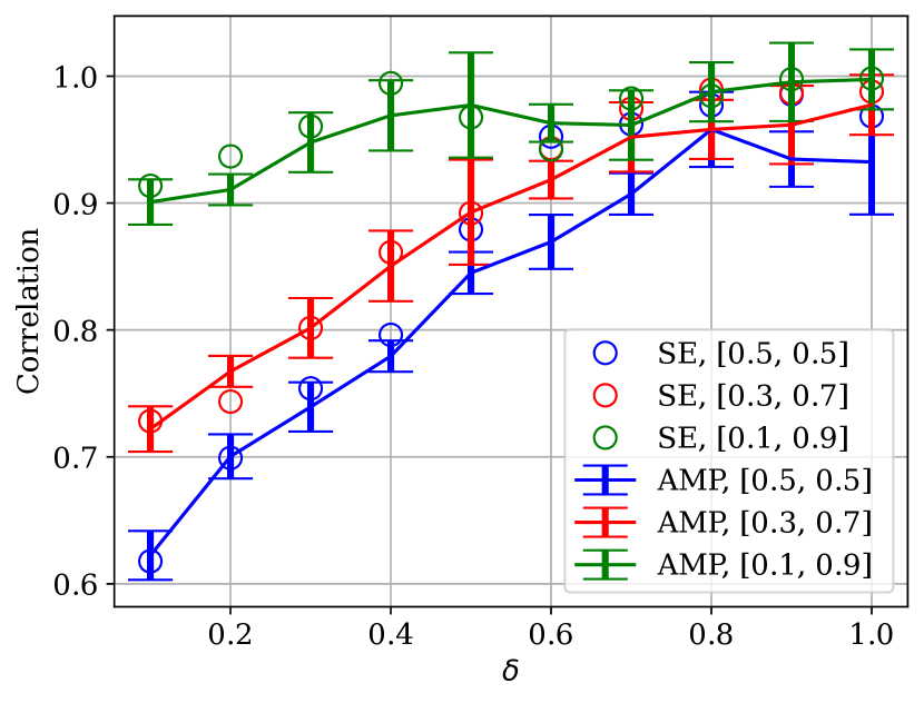
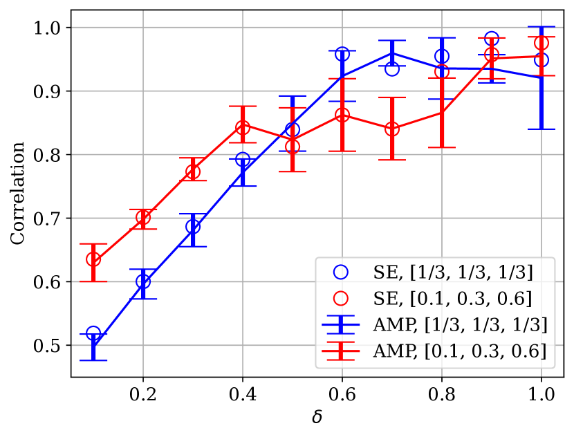
We present numerical simulation results for the pooled data model given by (3) (or equivalently (30)), in both the noiseless and noisy settings. We take $X_{ij}\stackrel{{\scriptstyle{\rm i.i.d.}}}{{\sim}}\text{Bernoulli}(\alpha)$ for $i,j\in[n]\times[p]$, and the rows of the signal $B_{j,:}\stackrel{{\scriptstyle{\rm i.i.d.}}}{{\sim}}\text{Categorical}(\pi)$ for $j\in[p]$, where $\pi$ is a vector of probabilities that sum to one. We use $\alpha=0.5$, since we find that the choice of $\alpha$ has very little effect on the performance of each algorithm. The rows of the initializer $\widehat{B}^{0}\in\mathbb{R}^{p\times 2}$ are chosen i.i.d. according to the same distribution $\pi$, independently of the signal. We set the signal dimension $p=500$ and vary the value of $n$ in our experiments. In all our plots, curves labeled ‘AMP’ refers to the empirical performance of the matrix-AMP algorithm, and points labeled ‘SE’ refers to the theoretical performance of the matrix-AMP algorithm, calculated from the state evolution parameters.

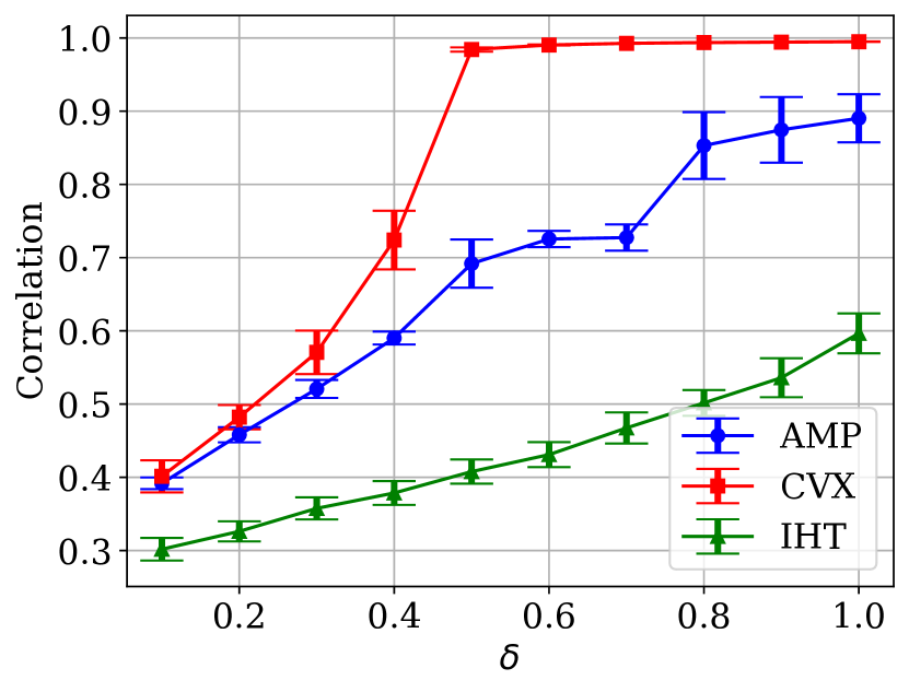
In the noisy setting, we consider Gaussian noise, with $\Psi_{i,:}\stackrel{{\scriptstyle{\rm i.i.d.}}}{{\sim}}\mathcal{N}(0,p\sigma^{2}I_{L})$ for $i\in[n]$. While it may seem unusual to add continuous noise to discrete observations, this still captures the essence of the noisy pooled data problem, and simplifies the implementation of our algorithm. Furthermore, since the noise standard deviation is of order $\sqrt{p}$, rounding the noise values to the nearest integer does not noticeably affect performance. This noisy model has been previously considered in [53, Section 2.2., Example 3].

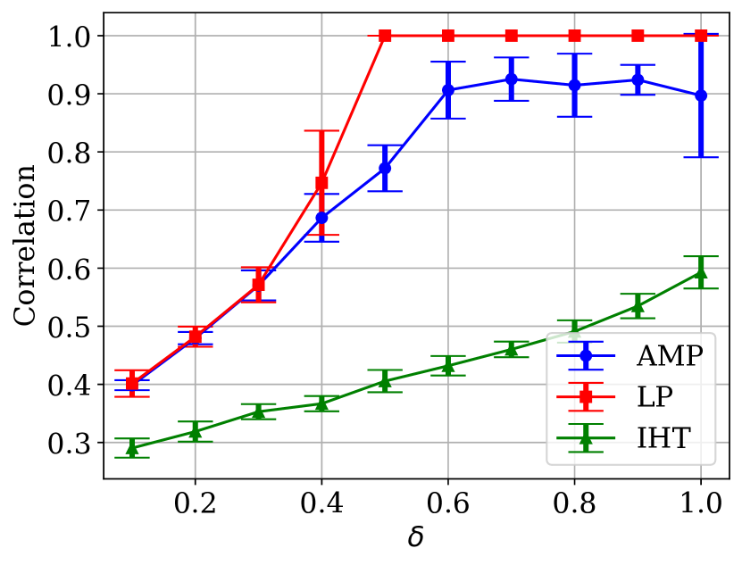
The matrix-AMP algorithm in (8) is implemented with $g_{k}=g_{k}^{*}$ and $f_{k}=f_{k}^{*}$, the optimal choices given by (25) and (24) respectively – see Appendix D.1 for details of the implementation. The performance in all the plots is measured via the normalized correlation between the matrix-AMP estimate and the signal (see (22)). Each point on the plots is obtained from 10 independent runs, where in each run, the matrix-AMP algorithm is executed for 10 iterations. We report the average and error bars at 1 standard deviation of the final iteration. In our implementation, in the final iteration of the matrix-AMP algorithm, we quantize the estimates of the signal $B$, e.g., a row estimate of $[0.9,0.1]$ would get quantized to $[1,0]$.

We also compare the matrix-AMP algorithm with two popular methods for compressed sensing: iterative hard thresholding and convex programming. Due to the additional constraints in the pooled data problem, some work is required to extend these algorithms to pooled data. The algorithms are defined as follows.

Optimization-based methods

We obtain these from the convex relaxation of the maximum a posteriori (MAP) estimator for pooled data. We assume that the categorical prior $\pi$ is known, i.e., the probability of each item belonging to category $l\in[L]$ is $\pi_{l}$. We first reformulate our variables to ones that are more suitable for optimization formulations. We define

$$Y_{\text{opt}} =\begin{bmatrix}Y_{:,1}\\ \vdots\\ Y_{:,L}\end{bmatrix}\in\mathbb{R}^{nL};\quad B_{\text{opt}}=\begin{bmatrix}B_{:,1}\\ \vdots\\ B_{:,L}\end{bmatrix}\in\{0,1\}^{pL};$$

(32) $$X_{\text{opt}} =\text{diag}(X,\dots,X)\in\{0,1\}^{nL\times pL};\quad C_{\text{opt}}=[I_{p},\dots,I_{p}]\in\{0,1\}^{p\times pL}.$$

Write $I_{pL}^{(pl)}\in\mathbb{R}^{l\times pl}$ for the sub-matrix of $I_{pL}$ obtained by taking the $p(l-1)$-th to $pl$-th rows of $I_{pL}$. The convex program for the noisy setting (CVX), with noise $\Psi_{i,:}\stackrel{{\scriptstyle{\rm i.i.d.}}}{{\sim}}\mathcal{N}(0,p\sigma^{2}I_{L})$, is

minimize $$\quad\frac{1}{2p\sigma^{2}}\|Y_{\text{opt}}-X_{\text{opt}}B_{\text{opt}}\|_{2}^{2}-\sum_{l=1}^{L}(\log\pi_{l})1_{p}^{\top}I_{pL}^{(pl)}B_{\text{opt}}\quad(\text{w.r.t.~{} $B_{\text{opt}}$})$$

subject to $$\quad 0_{p}\leq B_{\text{opt}}\leq 1_{p},\text{ and }C_{\text{opt}}B_{\text{opt}}=1_{p}.$$

For the noiseless pooled data setting, the convex program above can be simplified to the following linear program (LP):

minimize $$\quad-\sum_{l=1}^{L}(\log\pi_{l})1_{p}^{\top}I_{pL}^{(pl)}B_{\text{opt}}\quad(\text{w.r.t.~{} $B_{\text{opt}}$})$$

subject to $$\quad 0_{p}\leq B_{\text{opt}}\leq 1_{p},\,Y_{\text{opt}}=X_{\text{opt}}B_{\text{opt}},\,C_{\text{opt}}B_{\text{opt}}=1_{p}.$$

The derivations of the convex and linear programs are given in Appendix E.

Iterative hard thresholding

We extend the IHT algorithm [26, Section 3.3] for compressed sensing to pooled data. The algorithm is as follows:

• Input. $\widetilde{Y}$, $\widetilde{X}$, and the sparsity levels of the columns of $B$, namely $\{\pi_{1}^{*}p,\dots,\pi_{L}^{*}p\}$.

• Initialization. $B^{0}=0\in\mathbb{R}^{p\times L}$.

• For iteration $k=1,\dots,k_{\max}$: Execute

  $$B^{k+1}=H_{\{\pi_{1}^{*}p,\dots,\pi_{L}^{*}p\}}(B^{k}+\widetilde{X}^{\top}(\widetilde{Y}-\widetilde{X}B^{k})),$$

  where $H_{\{\pi_{1}^{*}p,\dots,\pi_{L}^{*}p\}}(\cdot)$ is the hard thresholding function adapted to matrix signals, and is defined to perform the following:

  • Look for the largest entry in the input matrix and make a hard decision on the corresponding (item, category) pair.

  • Once an item is allocated, it is removed from further consideration in the later iterations, and once a class $l$ has been allocated $\pi_{l}^{*}p$ items, we also remove it from further consideration in the later iterations.

• Return $B^{k_{\max}}$.

We found that that using $\widetilde{Y}$ and $\widetilde{X}$ instead of $Y$ and $X$ leads to better performance.

Simulation results

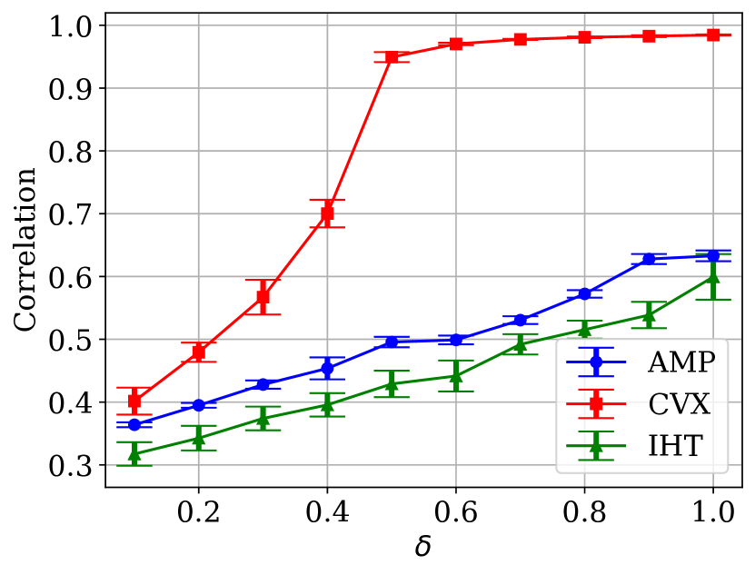
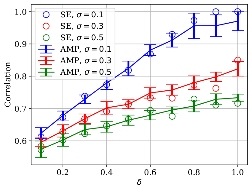
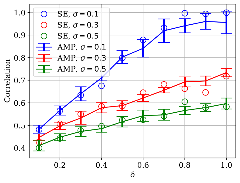
Figure 1 shows the performance of the matrix-AMP algorithm in the noiseless setting, for various $\pi$. The normalized correlation is plotted as function of the sampling ratio $\delta=n/p$, for different categorical priors. The state evolution predictions closely match the performance of the matrix-AMP algorithm for practical values of $n$ and $p$, validating the result of Theorem 3.2. As expected, the correlation improves with increasing $\delta$. Furthermore, we observe that for $L=2$, the more non-uniform the $\pi$, the better the performance of the matrix-AMP algorithm. However, this is not the case for $L=3$. Figure 2 shows how the matrix-AMP algorithm compares with LP and IHT for different noise levels. We observe that the optimization-based methods (LP for noiseless, CVX for noisy) outperforms the matrix-AMP algorithm, indicating the suboptimality of AMP in this setting. However, we note that there are currently no theoretical guarantees for LP or CVX applied to pooled data. Figure 3 shows the performance curves of the matrix-AMP algorithm for different values of noise level $\sigma$; as expected, correlation improves as $\sigma$ decreases.

(a) $L=2$.

(b) $L=3$.

Figure 1: AMP for pooled data: normalized correlation vs. $\delta$, with $\sigma=0$ and varying $\hat{\pi}$

(a) $\sigma=0$

(b) $\sigma=0.1$

(c) $\sigma=0.3$

Figure 2: AMP vs. other algorithms for pooled data: normalized correlation vs. $\delta$, with $L=3$ and $\hat{\pi}=[1/3,1/3,1/3]$. The plots are similar for the case of non-uniform priors.

(a) $L=2$

(b) $L=3$

Figure 3: AMP for pooled data: normalized correlation vs. $\delta$ for varying $\sigma$ with uniform prior $\pi$. The plots are similar for the case of non-uniform priors.

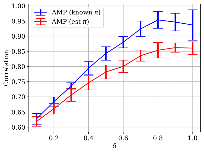
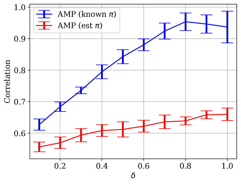
So far, we have assumed that the matrix-AMP algorithm has access to the empirical category proportions $\hat{\pi}$. We now study the performance when we do not know $\hat{\pi}$ exactly, but only have an estimate of it. For simplicity, we consider $L=2$ with estimated proportions $\pi_{\text{est}}=[\pi_{1}^{*}+\epsilon,\pi_{2}^{*}-\epsilon]$, for some $\epsilon>0$. Figure 4 shows the performance for $\epsilon=0.01$ and $\epsilon=0.05$. We observe that the performance of the matrix-AMP algorithm is very sensitive to the accuracy of the estimate $\pi_{\text{est}}$, i.e., a small increase in $\epsilon$ can substantially degrade the performance. The underlying reason that AMP requires each entry of $\widetilde{Y}$ to be of constant order (as $p$ grows) with high probability. This is true if $\hat{\pi}$ is known exactly; we show in Appendix F that $\mathbb{E}[\widetilde{Y}_{il}]=0$ and $\mathrm{Var}[\widetilde{Y}_{il}]=\frac{p\pi_{l}}{n}=\Theta(1)$, for $i\in[n],l\in[L]$. However, a constant shift of $\epsilon$ in the entries of $\hat{\pi}$ causes the the entries of $\widetilde{Y}$ to jump from $\Theta(1)$ to $\Theta(\sqrt{p})$ – see Appendix F for details. This indicates that it is worth performing additional (non-random) test(s) to obtain an accurate estimate of $\hat{\pi}$ before running the matrix-AMP algorithm.

(a) $\epsilon=0.01$

(b) $\epsilon=0.05$

Figure 4: Pooled data with mismatched proportions: normalized correlation vs. $\delta$ with $\hat{\pi}=[0.5,0.5]$ and $\sigma=0$. Red curves show AMP performance with the estimate $\pi_{\text{est}}=[\pi_{1}^{*}+\epsilon,\pi_{2}^{*}-\epsilon]$.

5 AMP for Quantitative Group Testing

Recall that Quantitative Group Testing (QGT) is a special case of the pooled data problem with $L=2$, where items are either defective or non-defective. As mentioned in Section 1.1, in QGT the signal is often represent by a vector $\beta\in\{0,1\}^{p}$, where $1$ corresponds to a ‘defective’ item and $0$ corresponds to a non-defective item. Using a vector instead of a $p\times 2$ matrix to represent the QGT signal has two major benefits: (i) It allows us to present guarantees for the false positive rate (FPR) and false negative rate (FNR) in a simpler way, and (ii) It provides a simpler and more efficient AMP algorithm where matrix operations can be omitted.

We use $\beta$ (instead of $B$) for the signal vector to avoid confusion between the pooled data problem and QGT. The design matrix is the same as that for pooled data, i.e., $X_{ij}\sim_{{\rm i.i.d.}}\text{Bernoulli}(\alpha)$ where $\alpha\in(0,1)$. The vector of test outcomes $Y\in\mathbb{R}^{n}$ is given by

(33) $$Y=X\beta\,+\,\Psi,\quad i\in[n],$$

where $\Psi\in\mathbb{R}^{n}$ is the additive noise. Recall that $\hat{\pi}$ is the proportion of defective items in the population. Substituting the decomposition of $X$ in (28) into (33) and rearranging, we get

$$\frac{Y-\alpha\boldsymbol{1}_{n}\boldsymbol{1}_{p}^{\top}\beta}{\sqrt{n\alpha(1-\alpha)}}=\widetilde{X}\beta+\frac{\Psi}{\sqrt{n\alpha(1-\alpha)}}.$$

Since $\alpha\boldsymbol{1}_{n}\boldsymbol{1}_{p}^{\top}\beta=\alpha p\left(\frac{1}{p}\boldsymbol{1}_{n}\boldsymbol{1}_{p}^{\top}\beta\right)=\alpha p[\hat{\pi},\dots,\hat{\pi}]^{\top}$, we can rewrite the noisy model as

(34) $$\frac{Y_{i}-\alpha p\hat{\pi}}{\sqrt{n\alpha(1-\alpha)}}=\widetilde{X}_{i,:}^{\top}\beta+\frac{\Psi_{i}}{\sqrt{n\alpha(1-\alpha)}},$$

which can be further rewritten as

(35) $$\widetilde{Y}_{i}=\widetilde{X}_{i,:}^{\top}\beta+\widetilde{\Psi}_{i},\quad i\in[n],\quad\text{ or }\quad\widetilde{Y}=\widetilde{X}\beta+\widetilde{\Psi}.$$

The noiseless QGT model can be obtained by setting $\Psi=0_{n}$.

5.1 Algorithm

As in the pooled data problem, we assume knowledge of $\hat{\pi}$ and apply the AMP algorithm with the modified data $\widetilde{X}$ and $\widetilde{Y}$. The AMP algorithm in (8) is used, noting that the iterates are vectors. To differentiate the AMP algorithm for QGT from the pooled data setting, we change notation, and replace $B,B^{k}$, and $\widehat{B}^{k}$, with $\beta,\beta^{k}$, and $\hat{\beta}^{k}$, respectively, for $k\geq 1$. The notation for state evolution parameters is also changed to emphasize that in QGT, they are scalars. We let $\mu_{\beta}^{k}:=\mathrm{M}_{B}^{k}$, $\sigma_{\beta}^{k}:=\mathrm{T}_{B}^{k}$, $\mu_{\Theta}^{k}:=\mathrm{M}_{\Theta}^{k}$, and $\sigma_{\Theta}^{k}:=\mathrm{T}_{\Theta}^{k}$.

We assume that the empirical distributions of $\beta\in\mathbb{R}^{p}$ and $\widetilde{\Psi}\in\mathbb{R}^{n}$ converge to well-defined limits as $p,n\to\infty$. Specifically, assume that $\beta\stackrel{{\scriptstyle W}}{{\rightarrow}}\bar{\beta}$ and $\widetilde{\Psi}\stackrel{{\scriptstyle W}}{{\rightarrow}}\bar{\Psi}$. Here $\bar{\beta}$ is a binary random variable whose law represents the limiting proportion of $1$s in $\beta$.

The AMP algorithm is initialized with a random $\hat{\beta}^{0}$ whose components are generated i.i.d. according to the law of $\bar{\beta}$. Then the initial covariance $\Sigma^{0}$ in (18) can be computed as:

$$\frac{1}{n}\begin{bmatrix}\beta^{\top}\beta&\beta^{\top}\hat{\beta}^{0}\\ (\hat{\beta}^{0})^{\top}\beta&(\hat{\beta}^{0})^{\top}\hat{\beta}^{0}\end{bmatrix}\,\stackrel{{\scriptstyle a.s.}}{{\rightarrow}}\,\frac{1}{\delta}\begin{bmatrix}\mathbb{E}\{\bar{\beta}^{2}\}&(\mathbb{E}\{\bar{\beta}\})^{2}\\ (\mathbb{E}\{\bar{\beta}\})^{2}&\mathbb{E}\{\bar{\beta}^{2}\}\end{bmatrix}=:\Sigma^{0}.$$

With these assumptions, Theorem 3.2 directly gives the following state evolution result.

Theorem 5.1.

Consider the AMP algorithm in (8) for the QGT model in (35), with the notational changes, assumptions, and initialization described above. Assume that the denoising functions $f_{k+1},g_{k}$ used in the AMP algorithm satisfy Assumption (A2) in Section 3.1. Then for each $k\geq 0$,

(36) $$\big{(}\beta,\beta^{0},\beta^{1},\dots,\beta^{k+1}\big{)} \stackrel{{\scriptstyle W_{2}}}{{\rightarrow}}\big{(}\bar{\beta},\bar{\beta}^{0},\mu^{1}_{\beta}\bar{\beta}+G^{1}_{\beta},\dots,\mu^{k+1}_{\beta}\bar{\beta}+G^{k+1}_{\beta}\big{)}$$

(37) $$\big{(}\widetilde{\Psi},\Theta,\Theta^{0},\dots,\Theta^{k}\big{)} \stackrel{{\scriptstyle W_{2}}}{{\rightarrow}}\big{(}\bar{\Psi},Z,\mu^{0}_{\Theta}\,Z+G^{0}_{\Theta},\dots,\mu^{k}_{\Theta}\,Z+G^{k}_{\Theta}\big{)},$$

almost surely as $n,p\to\infty$ with $n/p\to\delta$. Here $G_{\beta}^{k+1}\sim\mathcal{N}\big{(}0,\big{(}\sigma_{\beta}^{k+1}\big{)}^{2}\big{)}$ is independent of $\bar{\beta}$, and $G_{\Theta}^{k}\sim\mathcal{N}\big{(}0,\big{(}\sigma_{\Theta}^{k}\big{)}^{2}\big{)}$ is independent of $(Z,\bar{\Psi})$.

The optimal choices for the AMP denoising functions, given by $f_{k}^{*}$ and $g_{k}^{*}$ in (24) and (25), can be explicitly computed; see Appendix D.2. From the expressions, it is easy to verify that these functions satisfy Assumption (A2), as required by the theorem.

Performance measures

Theorem 5.1 allows us to compute the limiting values of performance measures such as the normalized squared correlation between the estimate $\hat{\beta}^{k}$ and the signal $\beta$. We have

(38) $$\frac{\langle\hat{\beta}^{k},\beta\rangle^{2}}{\|\hat{\beta}^{k}\|_{2}^{2}\|\beta\|_{2}^{2}}\stackrel{{\scriptstyle a.s.}}{{\rightarrow}}\frac{(\mathbb{E}[f_{k}(\mu_{\beta}^{k}\bar{\beta}+G_{\beta}^{k})\cdot\bar{\beta})])^{2}}{\mathbb{E}[f_{k}(\mu_{\beta}^{k}\bar{\beta}+G_{\beta}^{k})^{2}]\cdot\mathbb{E}[\bar{\beta}^{2}]}.$$

In practical applications of QGT, we might want to understand the false positive and false negative rates (FPR and FNR) separately, or weigh one more than the other based on the practical needs. We proceed to investigate the FPR and FNR of AMP estimates for QGT. To get a final estimate in the signal domain $\{0,1\}^{p}$, we can choose the denoiser $f_{k}$ in the final iteration $k=K$ to output a hard decision (whereas the $f_{k}$ in earlier iterations $1,\dots,K-1$ will have no such restriction). Theorem 5.1 guarantees that the empirical distribution of $\beta^{K}$ converges to the law of $\mu_{\beta}^{K}\bar{\beta}+G_{\beta}^{K}$. Therefore, for some chosen threshold $\zeta>0$, we define

(39) $$f_{K}(\beta^{K})=\mathds{1}\bigg{\{}\frac{\beta^{K}}{\mu_{\beta}^{K}}>\zeta\bigg{\}},$$

where the indicator function is applied component-wise to $\beta^{K}$. That is, the large entries of the input $\beta^{K}$ are declared to be one (i.e., defective) and small entries of $\beta^{K}$ to be zero (i.e., non-defective). Based on the above function, let us denote the estimated defective set by

(40) $$\widehat{\mathcal{S}}=\bigg{\{}j:\frac{\beta_{j}^{K}}{\mu_{\beta}^{k}}>\zeta\bigg{\}},$$

The FPR and the FNR are defined as follows:

(41) FPR $$=\frac{\sum_{j=1}^{p}\mathds{1}\{\beta_{j}=0\cap j\in\widehat{\mathcal{S}}\}}{p-\sum_{j=1}^{p}\beta_{j}},\quad\text{ and }\quad\text{FNR}=\frac{\sum_{j=1}^{p}\mathds{1}\{\beta_{j}=1\cap j\notin\widehat{\mathcal{S}}\}}{\sum_{j=1}^{p}\beta_{j}}.$$

Corollary 5.2.

Under the same assumptions as Theorem 5.1, applying the thresholding function in (39) in the final iteration $K>1$, we have

(42) $$\textup{FPR}\stackrel{{\scriptstyle a.s.}}{{\rightarrow}}1-\Phi\bigg{(}\frac{\mu_{\beta}^{K}}{\sigma_{\beta}^{K}}\zeta\bigg{)}\quad\text{ and }\quad\textup{FNR}\stackrel{{\scriptstyle a.s.}}{{\rightarrow}}1-\Phi\bigg{(}\frac{\mu_{\beta}^{K}}{\sigma_{\beta}^{K}}(1-\zeta)\bigg{)},$$

where $\Phi$ is the cumulative distribution function of the standard Gaussian distribution.

The proof of the corollary is given in Appendix C.

5.2 Numerical Simulations

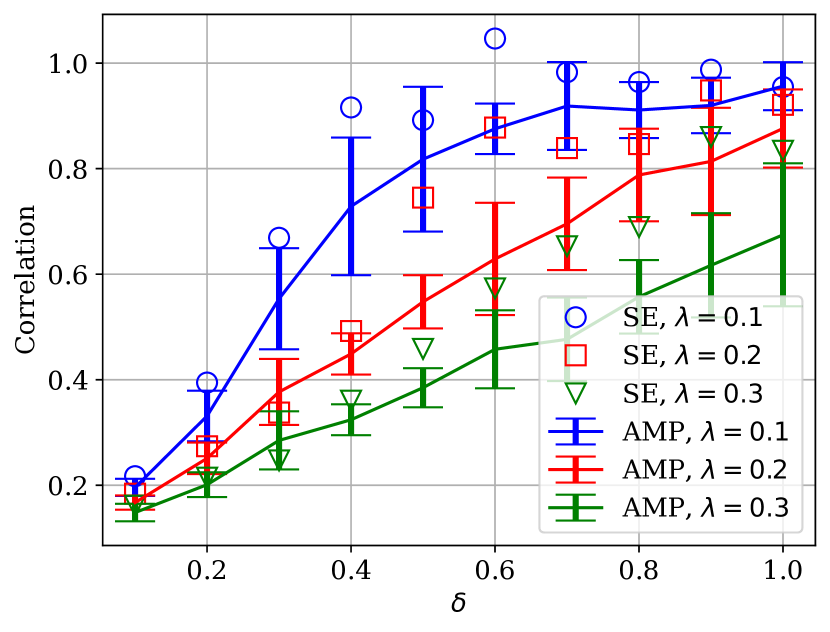
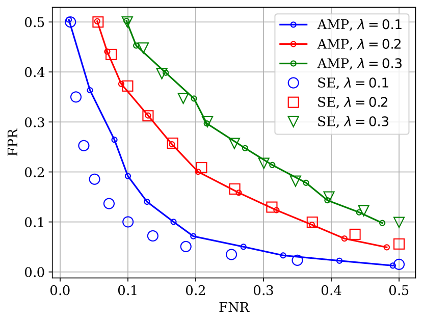
We present numerical simulation results for the QGT model in (33) (and equivalently (35)). We take $X_{ij}\stackrel{{\scriptstyle{\rm i.i.d.}}}{{\sim}}\text{Bernoulli}(0.5)$ for $i,j\in[n]\times[p]$ and $\beta_{j}\stackrel{{\scriptstyle{\rm i.i.d.}}}{{\sim}}\text{Bernoulli}(\pi)$ for $\pi\in(0,1)$ and $j\in[p]$; the initializer $\hat{\beta}^{0}\in\mathbb{R}^{p}$ is chosen randomly according to the same distribution as the signal vector $\beta$, but independent of it. For all our plots, the AMP algorithm in (8) is implemented with $g_{k}=g_{k}^{*}$ and $f_{k}=f_{k}^{*}$, with $f_{K}$ in (39) used in the final iteration $K$. The optimal choices $g_{k}^{*}$ and $f_{k}^{*}$ are given by (24) and (25); see Appendix D.2 for details of the implementation. The performance in all the plots is either measured via the normalized squared correlation between the AMP estimate and the signal (see (38)) or via the FPR and FNR (see (41)). We set the number of items to be $p=500$ and vary the value of the number of tests $n\leq p$ in our experiments. Each point on the plots is obtained from 10 independent runs, where in each run, the AMP algorithm is executed for 10 iterations. In the normalized squared correlation plots, we also report the average and error bars at 1 standard deviation of the final iteration.

Figure 5: QGT, FPR vs. FNR: We use $\alpha=0.5$, $\pi=0.1$, $p=500$, $\zeta\in\{0.1,0.2,\dots,1.0\}$.

QGT

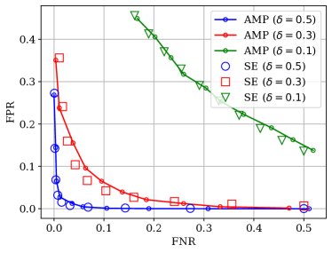
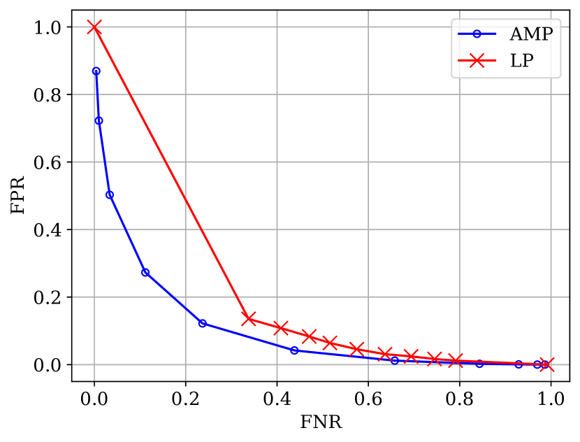
For the noiseless setting, Figure 5 shows that the FPR vs. FNR tradeoff curve improves (i.e., becomes lower) as $\delta$ increases (i.e., more tests are used). For all three curves, the theoretical results from Corollary 5.2 closely match the empirical result from the algorithm, giving an empirical verification of Theorem 5.1 and Corollary 5.2.

Our benchmark for the AMP algorithm will be linear programming (LP) estimator for the QGT problem. The optimization problem for LP is written as

minimize $$\|\beta\|_{1}$$

subject to $$y=X\beta,\text{ and }0\leq\beta_{j}\leq 1\text{ for }j\in[p].$$

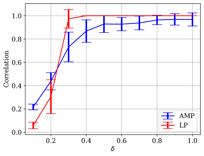
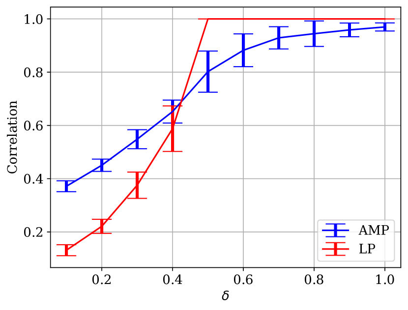
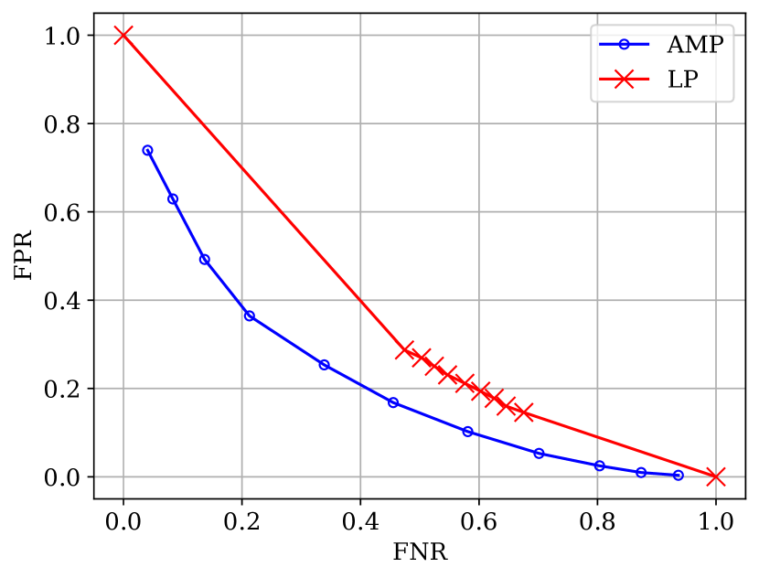
Similar reconstruction algorithms have been widely used in compressed sensing [26] and also studied for Boolean group testing [6]. Similar to the AMP algorithm, we can produce a FPR vs. FNR trade-off curve by using a thresholding function, with a varying threshold, to get the estimate of the signal. Specifically, after running the linear program to obtain $\beta^{(\text{lp})}$, we can set $\hat{\beta}_{j}=\mathds{1}\big{\{}\beta_{j}^{\text{(lp})}>\zeta\big{\}}$. Several other QGT algorithms have been proposed (some examples are [40, 39, 23, 35]) that were used for the sublinear category regime with no noise. We omit comparisons with them because they do not appear to offer a simple mechanism for controlling the trade-off between FPR and FNR. Figure 6 shows that LP outperforms the AMP algorithm for larger values of $\delta$, after $\delta=0.25$ for $\pi=0.1$, and after around the $\delta=0.55$ for $\pi=0.3$. Figure 7 shows the FPR vs. FNR tradeoff of the AMP algorithm and LP for $\pi=0.1$ and $\pi=0.3$, with sampling ratio $\delta=0.2$. These plots indicate that the AMP algorithm is better than LP when the sampling ratio $\delta$ is small and defective probability $\pi$ is large.

(a) Defective probability $\pi=0.1$

(b) $\pi=0.3$

Figure 6: QGT, Normalized squared correlation vs. $\delta$: We use $\alpha=0.5$ and $p=500$.

(a) $\pi=0.1$

(b) $\pi=0.3$

Figure 7: QGT, FPR vs. FNR: $\alpha=0.5$, $\delta=0.2$, $p=500$, and threshold $\zeta\in\{0,0.1,\dots,1.0\}$ for both AMP and LP.

Noisy QGT

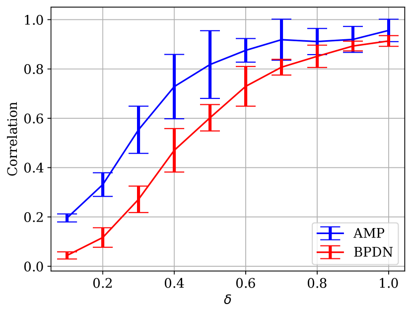
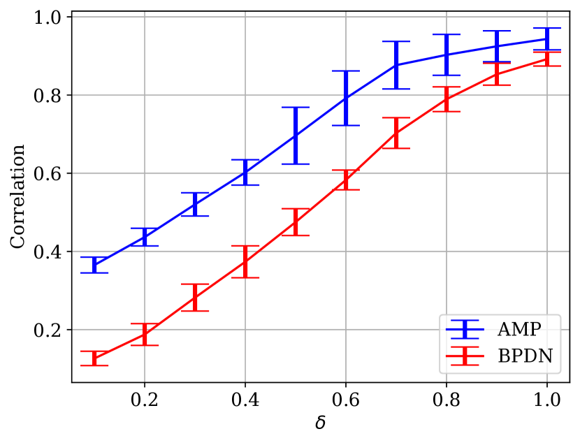
To highlight that the AMP algorithm works under different noise distributions, we consider QGT with uniformly distributed noise (recall that Gaussian noise was used for the pooled data simulations). Specifically, $\Psi_{i}\stackrel{{\scriptstyle{\rm i.i.d.}}}{{\sim}}\text{Uniform}[-\lambda\sqrt{p},\lambda\sqrt{p}]$ for some constant $\lambda$. After rescaling as in (35), we get $\widetilde{\Psi}_{i}={\widetilde{\Psi}_{i}}/{\sqrt{n\alpha(1-\alpha)}}$ whose empirical distribution converges to $\bar{\Psi}\sim\text{Uniform}[-\tilde{\lambda},\tilde{\lambda}]$, where $\tilde{\lambda}=\lambda/\sqrt{\delta\alpha(1-\alpha)}$. As expected, Figure 8 shows that performance of the AMP algorithm improves as the noise level $\lambda$ decreases.

(a) Norm. sq. correlation vs. $\delta$

(b) FPR vs. FNR

Figure 8: Noisy QGT with noise $\Psi_{i}\sim\text{Uniform}[-\lambda\sqrt{p},\lambda\sqrt{p}]$, normalized squared correlation vs. $\delta$ (left): We use $\alpha=0.5$, $\pi=0.1$, and $p=500$. FPR vs. FNR (right): We use $\alpha=0.5$, $\pi=0.1$, $\delta=0.3$, $p=500$, $\zeta\in\{0.1,0.2,\dots,1.0\}$.

Our benchmark for AMP will be a convex programming estimator that is a variant of basis pursuit denoising (BPDN) [13]. The convex program for BPDN can be written as

minimize $$\|\beta\|_{1}$$

subject to $$\|y-X\beta\|_{\infty}\leq\lambda\sqrt{p},\text{ and }0\leq\beta_{j}\leq 1\text{ for }j\in[p],$$

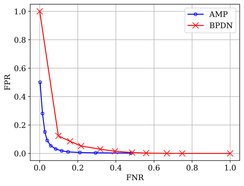
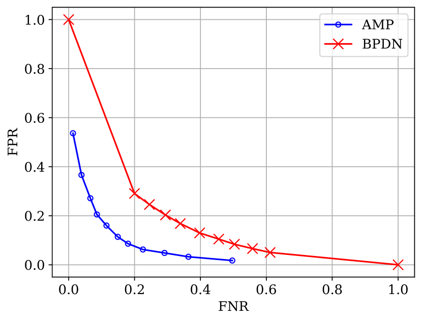
where the $\ell_{\infty}$-constraint is tailored to uniform noise. This BPDN-type algorithm is most commonly used in noisy compressed sensing. Similar to the AMP algorithm, we can obtain a FPR vs. FNR trade-off curve by using a thresholding function, with a varying threshold. Specifically, after running the convex program to obtain $\beta^{(\text{bpdn})}$, we can set $\hat{\beta}_{j}=\mathds{1}\big{\{}\beta_{j}^{\text{(bpdn})}>\zeta\big{\}}$. Figure 9 shows that the AMP algorithm outperforms BPDN for all values of $\delta$, and the performance gap is larger for smaller $\delta$. Figure 10 backs this up showing that the FPR vs. FNR curve for the AMP algorithm generally lies below that for BPDN, and the gap between the curves increases when $\pi$ is increased from $0.1$ to $0.3$.

(a) $\pi=0.1$

(b) $\pi=0.3$

Figure 9: Noisy QGT with noise $\Psi_{i}\sim\text{Uniform}[-\lambda\sqrt{p},\lambda\sqrt{p}]$, normalized squared correlation vs. $\delta$: $\alpha=0.5$, $\lambda=0.1$, and $p=500$.

(a) $\pi=0.1$

(b) $\pi=0.3$

Figure 10: Noisy QGT with noise $\Psi_{i}\sim\text{Uniform}[-\lambda\sqrt{p},\lambda\sqrt{p}]$, FPR vs. FNR: $\alpha=0.5$, $\lambda=0.1$, $\delta=0.5$, $p=500$, and $\zeta\in\{0,0.1,\dots,1.0\}$ for both AMP and BPDN.

6 Discussion and Future Directions

In this paper, we have obtained rigorous performance guarantees for the AMP algorithm applied to pooled data decoding and QGT, with i.i.d. Bernoulli design matrices. We expect that our analysis, based on the universality result of [67], can be extended to Bernoulli designs with additional structure (such as spatial coupling) that might help improve performance. The numerical results in Section 4.1 show that the convex programming estimator outperforms the AMP algorithm for pooled data with $L=3$. This is surprising, since it has been shown that for linear regression with i.i.d. Gaussian designs (and vector-valued signal), AMP with Bayes-optimal denoisers is superior to convex procedures for a large class of priors, and moreover, conjectured to be optimal among polynomial-time algorithms [12]. Obtaining rigorous theoretical guarantees for the convex pooled data estimator is an interesting direction for future work.

AMP for Boolean Group Testing

Recall that in noiseless BGT, the outcome of test $i\in[n]$ is $Y_{i}=\mathds{1}\{X_{i,:}^{\top}\beta>0\}$. As in QGT, the signal $\beta\in\mathbb{R}^{p}$ is binary vector, with ones in the entries corresponding to defective items. In the linear regime, where the number of defectives $d$ is proportional to $p$, it is known that individual testing is optimal for exact recovery [4, 8]. On the other hand, precisely characterizing the performance under an approximate recovery criterion, specifically the trade-off between FPR and FNR in the linear regime, is an open question [60]. The similarity between BGT and QGT suggests that the AMP analysis for the latter can be generalized to provide rigorous guarantees for BGT with i.i.d. Bernoulli matrices, similar to those of Theorem 5.1 for QGT. However, this is not the case. We briefly describe the challenges in extending our results to BGT.

Consider noiseless BGT with an i.i.d. $\text{Bernoulli}(\alpha)$ design matrix $X$. Using the decomposition in (26), we can rewrite (5) as the following re-centered and rescaled model:

$$Y_{i}=\mathds{1}\left\{\widetilde{X}_{i,:}^{\top}\beta>\frac{-\alpha p\hat{\pi}}{\sqrt{n\alpha(1-\alpha)}}\right\}=q(\widetilde{X}_{i,:}^{\top}\beta).$$

With $\widetilde{Y}_{i}:=Y_{i}$, this is a special case of the matrix-GLM model in (4). For each test in BGT to be informative (i.e., have a non-vanishing probability of being either positive or negative), we need $\alpha=\Theta\big{(}\frac{1}{p}\big{)}$, since the number of defectives is a constant fraction of $p$ [6, Section 2.1]. However, with this choice of $\alpha$, the re-centered and rescaled matrix $\widetilde{X}$ does not satisfy the second condition in Definition 3.1, which is required for rigorous AMP guarantees. In contrast, for QGT, the choice of $\alpha=\Theta(1)$ both leads to informative tests and gives an $\widetilde{X}$ satisfying all the conditions in Definition 3.1. We can attempt to overcome this issue by choosing $\alpha=\Theta\big{(}\frac{\log n}{n}\big{)}$, which ensures that $\widetilde{X}$ satisifes Definition 3.1, but this choice leads to uninformative tests. Intuitively, when $\alpha=\Theta\big{(}\frac{\log n}{n}\big{)}$, the average number of defective items in each test is of order $\frac{p\log n}{n}=\Theta(\log n)$ (where we used $n=\Theta(p)$), causing the test outcome to be positive with probability tending to $1$. That is, each individual test provides almost no information as $p$ grows large.

A potential solution would be to shift away from the linear regime where the number of defectives $d=\Theta(p)$, and instead apply the AMP algorithm to the mildly sublinear regime $d=\frac{p}{\log p}$. This would lead to each test being informative with $\alpha=\Theta\big{(}\frac{\log n}{n}\big{)}$, but does not satisfy the AMP assumption that requires the empirical distribution of the signal $\beta$ to converge to a well-defined limiting distribution. As a result, we would need to develop a new AMP algorithm that works for signals with sublinear sparsity – we leave this as an open problem.

Appendix A Proof of Theorem 3.2

We begin by stating the abstract AMP iteration from [67] for a generalized white noise matrix $\widetilde{X}\in\mathbb{R}^{n\times p}$, as defined in Definition 3.1. For $t\geq 1$, the iterates of the abstract AMP, denoted by $h^{t}\in\mathbb{R}^{p}$ and $e^{t}\in\mathbb{R}^{n}$, are produced using functions $f_{t}^{v}:\mathbb{R}^{t+2L}\rightarrow\mathbb{R}$, $f_{t+1}^{u}:\mathbb{R}^{t+L}\rightarrow\mathbb{R}$. Given an initializer $u^{1}\in\mathbb{R}^{n}$, side information $c^{1},\dots,c^{L_{\Psi}}\in\mathbb{R}^{n}$ and $d^{1},\dots,d^{2L}\in\mathbb{R}^{p}$, all independent of $\widetilde{X}$, the iterates of the abstract AMP are computed as:

(43) $$\begin{split}h^{t}&=\sqrt{\delta}\widetilde{X}^{\top}u^{t}-\sum_{s=1}^{t-1}b_{s}^{t}v^{s},\qquad v^{t}=f_{t}^{v}(h^{1},\dots,h^{t},d^{1},\dots,d^{2L})\\ e^{t}&=\sqrt{\delta}\widetilde{X}v^{t}-\sum_{s=1}^{t}a_{s}^{t}u^{s},\qquad u^{t+1}=f_{t+1}^{u}(e^{1},\dots,e^{t},c^{1},\dots,c^{L_{\Psi}}),\end{split}$$

where the memory coefficients $\{b_{s}^{t}\}_{s<t}$ and $\{a_{s}^{t}\}_{s\leq t}$ are defined below in (44). We note that the matrix $\widetilde{X}$ used in (43) has a different scaling to the one used in [67] – the $(i,j)$th entry of $\widetilde{X}$ variance $n^{-1}S_{ij}$ whereas [67] uses variance $p^{-1}S_{ij}$. This difference is accounted for by the $\sqrt{\delta}$ factor multiplying $\widetilde{X}$ and $\widetilde{X}^{\top}$ in (43).

Next, we have the following assumptions on the initializer and the side information vectors:

Assumption A.1.

When $n,p\rightarrow\infty$, we have $n/p=\delta\in(0,\infty)$, for fixed $L$. Furthermore, we have

$$(u^{1},c^{1},\dots,c^{L_{\Psi}})\stackrel{{\scriptstyle W}}{{\rightarrow}}(\bar{u}^{1},\bar{c}^{1},\dots,\bar{c}^{L_{\Psi}})\text{ and }(d^{1},\dots,d^{2L})\stackrel{{\scriptstyle W}}{{\rightarrow}}(\bar{d}^{1},\dots,\bar{d}^{2L}),$$

for joint limit laws $(\bar{u}^{1},\bar{c}^{1},\dots,\bar{c}^{L_{\Psi}})$ and $(\bar{d}^{1},\dots,\bar{d}^{2L})$ having finite moments of all orders, where $\mathbb{E}[(\bar{u}^{1})^{2}]\geq 0$. Multivariate polynomials are dense in the real $L^{2}$-spaces of functions $f:\mathbb{R}^{L_{\Psi}+1}\rightarrow\mathbb{R}$, $g:\mathbb{R}^{2L}\rightarrow\mathbb{R}$ with the inner-products

$$\langle f,\tilde{f}\rangle:=\mathbb{E}\big{[}f(\bar{u}^{1},\bar{c}^{1},\dots,\bar{c}^{L_{\Psi}})\tilde{f}(\bar{u}^{1},\bar{c}^{1},\dots,\bar{c}^{L_{\Psi}})\big{]}\text{ and }\langle g,\tilde{g}\rangle:=\mathbb{E}\big{[}g(\bar{d}^{1},\dots,\bar{d}^{2L})\tilde{g}(\bar{d}^{1},\dots,\bar{d}^{2L})\big{]}.$$

The state evolution result below states that the joint empirical distribution of $(h^{1},\ldots,h^{t})$ converges to a Gaussian law $\mathcal{N}(0,\Omega^{t})$. Similarly, the joint empirical distribution of $(e^{1},\ldots,e^{t})$ $\mathcal{N}(0,\Gamma^{t})$. The covariance matrices $\Omega^{t},\Gamma^{t}\in\mathbb{R}^{t\times t}$ are iteratively defined as follows, starting from $\Omega^{1}=\delta\mathbb{E}[(\bar{u}^{1})^{2}]\in\mathbb{R}^{1\times 1}$. Given $\Omega^{t}$, for $t\geq 1$, let $(\bar{h}^{1},\dots,\bar{h}^{t})\sim\mathcal{N}(0,\Omega^{t})$ independent of $(\bar{d}^{1},\dots,\bar{d}^{2L})$ and define

$$\bar{v}^{s}=f_{s}^{v}(\bar{h}^{1},\dots,\bar{h}^{s},\bar{d}^{1},\dots,\bar{d}^{2L}),\quad s\in[t].$$

Then, $\Gamma^{t}=(\mathbb{E}[\bar{v}^{r}\bar{v}^{s}])_{r,s=1}^{t}\in\mathbb{R}^{t\times t}$. Next, let $(\bar{e}^{1},\dots,\bar{e}^{t})\sim\mathcal{N}(0,\Gamma^{t})$ independent of $(\bar{u}^{1},\bar{c}^{1},\dots,$ $\bar{c}^{L_{\Psi}})$ and define

$$\bar{u}^{s+1}=f_{s+1}^{u}(\bar{e}^{1},\dots,\bar{e}^{s},\bar{c}^{1},\dots,\bar{c}^{L_{\Psi}}),\quad s\in[t].$$

Then, $\Omega^{t+1}=(\delta\cdot\mathbb{E}[\bar{u}^{r}\bar{u}^{s}])_{r,s=1}^{t+1}\in\mathbb{R}^{(t+1)\times(t+1)}$. We then define the memory coefficients in (43) as

(44) $$a_{s}^{t}=\mathbb{E}\big{[}\partial_{s}f_{t}^{v}(\bar{h}^{1},\dots,\bar{h}^{t},\bar{d}^{1},\dots,\bar{d}^{2L})\big{]}\text{ and }b_{s}^{t}=\delta\cdot\mathbb{E}\big{[}\partial_{s}f_{t}^{u}(\bar{e}^{1}.\dots,\bar{e}^{t-1},\bar{c}^{1},\dots,\bar{c}^{L})\big{]},$$

where $\partial_{s}$ denotes partial derivative in the $s$th argument. The following theorem gives the state evolution result for the abstract AMP iteration.

Theorem A.2.

[67, Theorem 2.17] Let $\widetilde{X}\in\mathbb{R}^{n\times p}$ be a generalized white noise matrix (as defined in Definition 3.1) with variance profile $S\in\mathbb{R}^{n\times p}$, and let $u^{1},c^{1},\dots,c^{L_{\Psi}},d^{1},\dots,d^{2L}$ be independent of $\widetilde{X}$ and satisfy Assumption A.1. Suppose that

1. Each function $f_{t}^{v}:\mathbb{R}^{t+2L}\rightarrow\mathbb{R}$ and $f_{t+1}^{u}:\mathbb{R}^{t+L}\rightarrow\mathbb{R}$ is continuous, is Lipschitz in its first $t$ arguments, and satisfies the polynomial growth condition in (6) for some order $r\geq 1$.

2. $\|\widetilde{X}\|_{\textup{op}}<C$, for some constant $C$ almost surely for all large $n$ and $p$.

3. For any fixed polynomial functions $f^{\dagger}:\mathbb{R}^{L_{\Psi}+1\rightarrow\mathbb{R}}$ and $f^{\ddagger}:\mathbb{R}^{2L}\rightarrow\mathbb{R}$, almost surely as $n,p\rightarrow\infty$,

   $$\max_{i=1}^{n}\left|\langle f^{\dagger}(u^{1},c^{1},\dots,c^{L_{\Psi}})\odot S_{i,:}\rangle-\langle f^{\dagger}(u^{1},c^{1},\dots,c^{L_{\Psi}})\rangle\cdot\langle S_{i,:}\rangle\right|\rightarrow 0$$

   $$\max_{j=1}^{p}\left|\langle f^{\ddagger}(d^{1},\dots,d^{2L})\odot S_{:,j}\rangle-\langle f^{\ddagger}(d^{1},\dots,d^{2L})\rangle\cdot\langle S_{:,j}\rangle\right|\rightarrow 0,$$

Then for any fixed $t\geq 1$, where each matrix $\Omega^{t}$ and $\Gamma^{t}$ is positive semidefinite, almost surely as $n,p\rightarrow\infty$ with $n/p=\delta\in(0,\infty)$, the iterates of the abstract AMP in (43) satisfy

$$(u^{1},c^{1},\dots,c^{L_{\Psi}},e^{1},\dots,e^{t})\stackrel{{\scriptstyle W_{2}}}{{\rightarrow}}(\bar{u}^{1},\bar{c}^{1},\dots,\bar{c}^{L_{\Psi}},\bar{e}^{1},\dots,\bar{e}^{t})$$

$$(d^{1},\dots,d^{2L},h^{1},\dots,h^{t})\stackrel{{\scriptstyle W_{2}}}{{\rightarrow}}(\bar{d}^{1},\dots,\bar{d}^{2L},\bar{h}^{1},\dots,\bar{h}^{t}),$$

where $(\bar{h}^{1},\dots,\bar{h}^{t})\sim\mathcal{N}(0,\Omega^{t})$ and $(\bar{e}^{1},\dots,\bar{e}^{t})\sim\mathcal{N}(0,\Gamma^{t})$ are independent of $(\bar{u}^{1},\bar{c}^{1}.\dots,\bar{c}^{L_{\Psi}})$ and $\bar{d}^{1},\dots,\bar{d}^{2L}$.

The theorem above shows that the state evolution result for an abstract AMP iteration defined via a generalized white noise matrix is the same as the one for an i.i.d. Gaussian matrix (where $\widetilde{X}_{ij}\stackrel{{\scriptstyle{\rm i.i.d.}}}{{\sim}}\mathcal{N}(0,\frac{1}{n})$), which was previously given in [36].

A.1 Reduction of matrix-AMP to abstract AMP

We now inductively map the iterates of matrix-AMP (8) to iterates of the abstract AMP. At each step of the induction, there are two main reductions:

• Reduction of the matrix-AMP iterates to the abstract AMP iterates;

• Reduction of the matrix-AMP SE parameters to the abstract AMP SE parameters.

Recalling that each matrix-AMP iterate has $L$ columns, for the first matrix-AMP iteration, we need $4L$ abstract AMP iterations to represent each matrix-AMP iteration. For subsequent matrix-AMP iterations, we need $2L$ abstract AMP iterations to represent each matrix-AMP iteration.

We will prove Theorem 3.2 for a slightly modified version of the matrix-AMP algorithm, where the matrices $C^{k}$ and $F^{k+1}$ in (3.1) are replaced by their deterministic versions, defined in (46) below. The state evolution result remains valid for the matrix-AMP algorithm in (8), by standard arguments in Remark 2.19 of [67].

Starting with an initialization $\widehat{B}^{0}\in\mathbb{R}^{p\times L}$ and defining $\widehat{R}^{-1}:=0\in\mathbb{R}^{n\times L}$, for iteration $k\geq 0$ the matrix-AMP algorithm with deterministic memory coefficient matrices computes:

(45) $$\begin{split}&\Theta^{k}=\widetilde{X}\widehat{B}^{k}-\widehat{R}^{k-1}(F^{k})^{\top},\quad\widehat{R}^{k}=g_{k}(\Theta^{k},\widetilde{Y}),\\ &B^{k+1}=\widetilde{X}^{\top}\widehat{R}^{k}-\widehat{B}^{k}(C^{k})^{\top},\quad\widehat{B}^{k+1}=f_{k+1}(B^{k+1}).\end{split}$$

The deterministic matrices $C^{k},F^{k+1}\in\mathbb{R}^{L\times L}$ are defined as

(46) $$C^{k}=\mathbb{E}\big{[}g_{k}^{\prime}(Z^{k},\bar{Y})\big{]},\quad F^{k+1}=\frac{1}{\delta}\mathbb{E}\big{[}f_{k+1}^{\prime}(\mathrm{M}_{B}^{k+1}\bar{B}+G_{B}^{k+1})\big{]},$$

where $g_{k}^{\prime},f_{k+1}^{\prime}$ denote the Jacobians of $g_{k},f_{k+1}$, respectively, with respect to their first arguments.

Initialization of abstract AMP: We let $u^{1}=0$, and define the side information vectors

$$d^{1}=B_{:,1},\dots,\,d^{L}=B_{:,L},\,d^{L+1}=\widehat{B}^{0}_{:,1},\dots,\,d^{2L}=\widehat{B}^{0}_{:,L}\,,$$

(47) $$c^{1}=\widetilde{\Psi}_{:,1},\dots,\,c^{L_{\Psi}}=\widetilde{\Psi}_{:,L_{\Psi}}.$$

Base case: We consider the case $k=0$, and our goal is to reduce $\widehat{B}^{0}$, $\Theta^{0}$, $B^{1}$, $\widehat{R}^{0}$, $\widehat{B}^{1}$, and $\Theta^{1}$ to abstract AMP iterates, via careful choices of the functions $f^{v}_{t}$ and $f^{u}_{t+1}$. This requires $4L$ abstract AMP iterations. We give a summary of the reductions below, and then provide detailed derivations:

• For $t=1$:

  (48) $$\begin{split}h^{1}=0;\quad v^{1}=\frac{1}{\sqrt{\delta}}B_{:,1};\quad e^{1}=\Theta_{:,1};\quad u^{2}=0\end{split}$$

• For $t=2,\dots,L$:

  (49) $$\begin{split}&h^{2},\dots,h^{L}=0;\quad\big{(}v^{2},\dots,v^{L}\big{)}=\frac{1}{\sqrt{\delta}}\big{(}B_{:,2},\dots,B_{:,L});\\ &\big{(}e^{2},\dots,e^{L})=\big{(}\Theta_{:,2},\dots,\Theta_{:,L}\big{)};\quad u^{3},\dots,u^{L+1}=0.\end{split}$$

• For $t=L+1,\dots,2L-1$:

  (50) $$\begin{split}&h^{L+1},\dots,h^{2L-1}=0;\quad\big{(}v^{L+1},\dots,v^{2L-1}\big{)}=\frac{1}{\sqrt{\delta}}\Big{(}\widehat{B}_{:,1}^{0},\dots,\widehat{B}_{:,L-1}^{0}\Big{)};\\ &\big{(}e^{L+1},\dots,e^{2L-1}\big{)}=\Big{(}\Theta_{:,1}^{0},\dots,\Theta_{:,L-1}^{0}\Big{)};\quad u^{L+1},\dots,u^{2L}=0.\end{split}$$

• For $t=2L$:

  (51) $$\begin{split}h^{2L}=0;\quad v^{2L}=\frac{1}{\sqrt{\delta}}\widehat{B}_{:,L}^{0};\quad e^{2L}=\Theta_{:,L}^{0};\quad u^{2L+1}=\frac{1}{\sqrt{\delta}}\widehat{R}_{:,1}^{0}.\end{split}$$

• For $t=2L+1,\dots,3L-1$:

  (52) $$\begin{split}&\big{(}h^{2L+1},\dots,h^{3L-1}\big{)}=\Big{(}B_{:,1}^{1}-\{B(\mathrm{M}_{B}^{1})^{\top}\}_{:,1},\dots,B_{:,L-1}^{1}-\{B(\mathrm{M}_{B}^{1})^{\top}\}_{:,L-1}\Big{)};\\ &v^{2L+1},\dots,v^{3L-1}=0;\\ &e^{2L+1},\dots,e^{3L-1}=0;\quad\big{(}u^{2L+2},\dots,u^{3L}\big{)}=\frac{1}{\sqrt{\delta}}\Big{(}\widehat{R}_{:,2}^{0},\dots,\widehat{R}_{:,L}^{0}\Big{)}.\end{split}$$

• For $t=3L$:

  (53) $$\begin{split}h^{3L}=B_{:,L}^{1}-\{B(\mathrm{M}_{B}^{1})^{\top}\}_{:,L};\quad v^{3L}=0;\quad e^{3L}=0;\quad u^{3L+1}=0.\end{split}$$

• For $t=3L+1,\dots,4L-1$:

  (54) $$\begin{split}&h^{3L+1},\dots,h^{4L-1}=0;\quad\big{(}v^{3L+1},\dots,v^{4L-1}\big{)}=\frac{1}{\sqrt{\delta}}\Big{(}\widehat{B}_{:,1}^{1},\dots,\widehat{B}_{:,L-1}^{1}\Big{)};\\ &\big{(}e^{3L+1},\dots,e^{4L-1}\big{)}=\Big{(}\Theta_{:,1}^{1},\dots,\Theta_{:,L-1}^{1}\Big{)};\quad u^{3L+2},\dots,u^{4L}=0.\end{split}$$

• For $t=4L$:

  (55) $$\begin{split}h^{4L}&=0;\quad v^{4L}=\frac{1}{\sqrt{\delta}}\widehat{B}_{:,L}^{1};\quad e^{4L}=\Theta_{:,L}^{1};\quad u^{4L+1}=\frac{1}{\sqrt{\delta}}\widehat{R}_{:,1}^{1}.\end{split}$$

We now provide the detailed derivations of (48)-(55). For $t=1,\dots,L+1$, define

(56) $$f_{t}^{v}(h^{1},\dots,h^{L},d^{1},\dots,d^{2L})=\frac{1}{\sqrt{\delta}}d^{t},\ \text{ and }\ f_{t+1}^{u}(e^{1},\dots,e^{t},c^{1},\dots,c^{L_{\Psi}})=0.$$

For $t=1$, using $u^{1}=0$, this gives

$$h^{1}=0;\quad v^{1}=f_{1}^{v}(h^{1},d^{1},\dots,d^{2L})=\frac{1}{\sqrt{\delta}}d^{1}=\frac{1}{\sqrt{\delta}}B_{:,1};$$

$$e^{1}=\sqrt{\delta}\widetilde{X}v^{1}-a_{1}^{1}u^{1}=\widetilde{X}B_{:,1}\,;\quad u^{2}=f_{2}^{u}(e^{1},c^{1},\dots,c^{L_{\Psi}})=0,$$

giving us (48). For $t=2$, using (56) we have

$$h^{2}=\sqrt{\delta}\widetilde{X}^{\top}u^{2}-b_{1}^{2}v^{1}=0\,;\quad v^{2}=f_{2}^{v}(h^{1},h^{2},d^{1},\dots,d^{2L})=\frac{1}{\sqrt{\delta}}d^{2}=\frac{1}{\sqrt{\delta}}B_{:,2}\,;$$

$$e^{2}=\sqrt{\delta}\widetilde{X}v^{2}-\sum_{s=1}^{2}a_{s}^{2}u^{s}=\widetilde{X}B_{:,2}\,;\quad u^{3}=f_{3}^{u}(e^{1},e^{2},c^{1},\dots,c^{L_{\Psi}})=0.$$

A similar derivation follows for $t=3,\dots,L$ to give

$$h^{t}=0;\quad v^{t}=\frac{1}{\sqrt{\delta}}B_{:,t};\quad e^{t}=\widetilde{X}B_{:,t};\quad u^{t+1}=0.$$

This completes the derivation of (49). For $t=L+1$, we have

$$h^{L+1} =\sqrt{\delta}\widetilde{X}^{\top}u^{L+1}-\sum_{s=1}^{L}b^{L+1}_{s}v^{s}\stackrel{{\scriptstyle(a)}}{{=}}0\,;$$

$$v^{L+1} =f_{L+1}^{v}(h^{1},\dots,h^{L+1},d^{1},\dots,d^{2L})=\frac{1}{\sqrt{\delta}}d^{L+1}=\frac{1}{\sqrt{\delta}}\widehat{B}^{0}_{:,1}\,;$$

$$e^{L+1} =\sqrt{\delta}\widetilde{X}v^{L+1}-\sum_{s=1}^{L+1}a^{L+1}_{s}u^{s}\stackrel{{\scriptstyle(b)}}{{=}}\widetilde{X}\widehat{B}_{:,1}^{0}\,;$$

$$u^{L+2} =f_{L+2}^{u}(e^{1},\dots,e^{L+1},c^{1},\dots,c^{L_{\Psi}})=0\,;$$

Here (a) uses $u^{L+1}=0$ and $b_{s}^{L+1}=0$ (because $f_{L+1}^{u}=0$), and (b) uses $u^{1},\dots,u^{L+1}=0$.

For $t=L+2,\dots,2L-1$, let us define

(57) $$f_{t}^{v}(h^{1},\dots,h^{L},d^{1},\dots,d^{2L})=\frac{1}{\sqrt{\delta}}d^{t-L}\text{ and }f_{t+1}^{u}(e^{1},\dots,e^{t},c^{1},\dots,c^{L_{\Psi}})=0.$$

Then, a similar derivation follows for $t=L+2,\dots,2L-1$ to give

$$h^{t}=0;\quad v^{t}=\frac{1}{\sqrt{\delta}}\widehat{B}^{0}_{:,t-L};\quad e^{t}=\widetilde{X}\widehat{B}^{0}_{:,t-L};\quad u^{t+1}=0.$$

This completes the derivation of (50). For $t=2L$, define

(58) $$\begin{split}&f_{2L}^{v}(h^{1},\dots,h^{2L},d^{1},\dots,d^{2L})=\frac{1}{\sqrt{\delta}}d^{2L},\\ &f_{2L+1}^{u}(\underbrace{e^{1},\dots,e^{L}}_{\widetilde{X}B=\Theta},\underbrace{e^{L+1},\dots,e^{2L}}_{\widetilde{X}\widehat{B}^{0}=\Theta^{0}},\underbrace{c^{1},\dots,c^{L_{\Psi}}}_{\widetilde{\Psi}})=\frac{1}{\sqrt{\delta}}\big{\{}g_{0}(\Theta^{0},q(\Theta,\widetilde{\Psi}))\big{\}}_{:,1}.\end{split}$$

Using this, we have

$$h^{2L}=\sqrt{\delta}\widetilde{X}^{\top}u^{2L}-\sum_{s=1}^{2L-1}b_{s}^{2L}v^{s}\stackrel{{\scriptstyle(a)}}{{=}}0;$$

$$v^{2L}=f_{2L}^{v}(h^{1},\dots,h^{2L},d^{1},\dots,d^{2L})=\frac{1}{\sqrt{\delta}}d^{2L}=\frac{1}{\sqrt{\delta}}\widehat{B}^{0}_{:,L};$$

$$e^{2L}=\sqrt{\delta}\widetilde{X}v^{2L}-\sum_{s=1}^{2L}a_{s}^{2L}u^{s}\stackrel{{\scriptstyle(b)}}{{=}}\widetilde{X}\widehat{B}^{0}_{:,L};$$

$$u^{2L+1}=f_{2L+1}^{u}(e^{1},\dots,e^{L},e^{L+1},\dots,e^{2L},c^{1},\dots,c^{L_{\Psi}})=\frac{1}{\sqrt{\delta}}\big{\{}g_{0}(\Theta^{0},q(\Theta,\widetilde{\Psi}))\big{\}}_{:,1}=\frac{1}{\sqrt{\delta}}\widehat{R}_{:,1}^{0}\,.$$

Here (a) applies $u^{2L}=0$ and $b_{s}^{2L}=0$ (because $f_{2L}^{u}=0$), and (b) applies $u^{1},\dots,u^{2L}=0$. This completes the derivation of (51).

For $t=2L+1,\ldots,3L-1$, we define

(59) $$\begin{split}&f_{t}^{v}(h^{1},\dots,h^{t},d^{1},\dots,d^{2L})=0,\\ &f_{t+1}^{u}(e^{1},\dots,e^{t},c^{1},\dots,c^{L_{\Psi}})=\frac{1}{\sqrt{\delta}}\big{\{}g_{0}(\Theta^{0},q(\Theta,\widetilde{\Psi}))\big{\}}_{:,t+1-2L}.\end{split}$$

For $t=2L+1$, using (46) we first write the first column of the term $\{\widehat{B}^{0}(C^{0})^{\top}\}$ as

(60) $$\{\widehat{B}^{0}(C^{0})^{\top}\}_{:,1} =\widehat{B}^{0}\cdot\begin{bmatrix}\mathbb{E}[\partial_{1}g_{0,1}(Z^{0},\bar{Y})]\\ \vdots\\ \mathbb{E}[\partial_{L}g_{0,1}(Z^{0},\bar{Y})]\end{bmatrix}=\sum_{l=1}^{l}\widehat{B}_{:,l}^{0}\mathbb{E}[\partial_{l}g_{0,1}(Z^{0},\bar{Y})],$$

where $g_{0,1}$ refers to the first entry of the output of $g_{0}$. We then have

$$h^{2L+1} =\sqrt{\delta}\widetilde{X}^{\top}u^{2L+1}-\sum_{s=1}^{L}b_{s}^{2L+1}v^{s}-\sum_{s=L+1}^{2L}b_{s}^{2L+1}v^{s}$$

$$=\sqrt{\delta}\widetilde{X}^{\top}u^{2L+1}-\sum_{s=1}^{L}\delta\mathbb{E}[\partial_{s}f_{2L+1}^{u}(\bar{e}^{1},\dots,\bar{e}^{2L},\bar{c}^{1},\dots,\bar{c}^{L_{\Psi}})]v^{s}$$

$$\qquad-\sum_{s=L+1}^{2L}\delta\mathbb{E}\big{[}\partial_{s}f_{2L+1}^{u}(\bar{e}^{1},\dots,\bar{e}^{2L},\bar{c}^{1},\dots,\bar{c}^{L_{\Psi}})\big{]}v^{s}$$

$$\stackrel{{\scriptstyle(a)}}{{=}}\widetilde{X}\widehat{R}_{:,1}^{0}-\sum_{l=1}^{L}\mathbb{E}\big{[}\partial_{l}\tilde{g}_{0,1}(Z,Z^{0},\bar{Y})\big{]}B_{:,l}-\sum_{l=1}^{L}\mathbb{E}\big{[}\partial_{l}g_{0,1}(Z,Z^{0},\bar{Y})\big{]}\widehat{B}_{:,l}^{0}$$

$$\stackrel{{\scriptstyle(b)}}{{=}}B_{:,1}^{1}-\{B(\mathrm{M}_{B}^{k})\}_{:,1},$$

where (a) applies $u^{2L+1}=\frac{1}{\sqrt{\delta}}\widehat{R}_{:,1}^{0}$, $v^{s}=\frac{1}{\sqrt{\delta}}B_{:,s}$ for $s\in[L]$, $v^{s}=\frac{1}{\sqrt{\delta}}\widehat{B}^{0}_{:,s}$ for $s\in[L+1:2L]$, and

$$u^{2L+1} =f_{2L+1}^{u}(e^{1},\dots,e^{2L},c^{1},\dots,c^{L_{\Psi}})=\frac{1}{\sqrt{\delta}}g_{0,1}(\Theta^{0},q(\Theta,\widetilde{\Psi}))=\frac{1}{\sqrt{\delta}}\tilde{g}_{0,1}(\Theta,\Theta^{0},\widetilde{\Psi})$$

$$\implies\bar{u}^{2L+1} =f_{2L+1}^{u}(\bar{e}^{1},\dots,\bar{e}^{2L},\bar{c}^{1},\dots,\bar{c}^{L_{\Psi}})=\frac{1}{\sqrt{\delta}}\tilde{g}_{0,1}(Z,Z^{0},\bar{\Psi}).$$

The equality (b) applies (60) and $B_{:,1}^{1}=\widetilde{X}\widehat{R}_{:,1}^{0}-\{\widehat{B}^{0}(C^{0})^{\top}\}_{:,1}$. Next, using (59) we have

$$v^{2L+1} =f_{2L+1}^{v}(h^{1},\dots,h^{2L+1},d^{1},\dots,d^{2L})=0\,,$$

$$e^{2L+1} =\widetilde{X}v^{2L+1}-\sum_{s=1}^{2L+1}a^{2L+1}_{s}u^{s}\stackrel{{\scriptstyle(a)}}{{=}}0\,,$$

$$u^{2L+2} =f_{2L+2}^{u}(e^{1},\dots,e^{2L+1},c^{1},\dots,c^{L_{\Psi}}):=\frac{1}{\sqrt{\delta}}\big{\{}g_{0}(\Theta^{0},q(\Theta,\widetilde{\Psi}))\big{\}}_{:,2}=\frac{1}{\sqrt{\delta}}\widehat{R}_{:,2}^{0}\,,$$

where (a) applies $v^{2L+1}=0$ and $a^{2L+1,s}=0$ (because $f_{2L+1}^{v}=0$). A similar derivation follows for $t=2L+2,\dots,3L-1$ to give

$$h^{t}=B^{1}_{:,t-2L}-\{B(\mathrm{M}_{B}^{k})^{\top}\}_{:,t-2L};\quad v^{t}=0;\quad e^{t}=0;\quad u^{t+1}=\frac{1}{\sqrt{\delta}}\widehat{R}_{:,t+1-2L}^{0}.$$

This completes the derivation of (52). For $t=3L$, we have

$$h^{3L} =\sqrt{\delta}\widetilde{X}^{\top}u^{3L}-\sum_{s=1}^{3L-1}b^{3L}_{s}v^{s}$$

$$=\sqrt{\delta}\widetilde{X}^{\top}u^{3L}-\sum_{s=1}^{2L}b^{3L}_{s}v^{s}-\sum_{s=2L+1}^{3L-1}b^{3L}_{s}\underbrace{v^{s}}_{=0}$$

$$=B_{:,L}^{1}-\{B(\mathrm{M}_{B}^{k})^{\top}\}_{:,L},$$

where the final equality applies (60) and $B_{:,L}^{1}=\widetilde{X}\widehat{R}_{:,L}^{0}-\{\widehat{B}^{0}(C^{0})^{\top}\}_{:,L}$. Next, we define both $f_{3L}^{v}$ and $f_{3L+1}^{u}$ to be 0, so that

$$v^{3L} =f_{3L}^{v}(h^{1},\dots,h^{3L},d^{1},\dots,d^{2L})=0$$

$$e^{3L} =\widetilde{X}\underbrace{v^{3L}}_{=0}-\sum_{s=1}^{3L}\underbrace{a^{3L}_{s}}_{=0}u^{s}=0$$

$$u^{3L+1} =f_{3L+1}^{u}(e^{1},\dots,e^{3L},c^{1},\dots,c^{L_{\Psi}})=0.$$

This completes the derivation of (53).

For $t=3L+1,\ldots,4L-1$, we define

(61) $$\begin{split}&f_{t}^{v}(h^{1},\dots,h^{2L},\underbrace{h^{2L+1},\dots,h^{3L}}_{B^{1}-B(\mathrm{M}_{B}^{1})^{\top}},h^{3L+1},\ldots,h^{t},\underbrace{d^{1},\dots,d^{2L}}_{B,\widehat{B}^{0}})=\frac{1}{\sqrt{\delta}}\{f_{1}(B^{1})\}_{:,t-3L},\\ &f_{t+1}^{u}(e^{1},\ldots,e^{t},c^{1},\dots,c^{L_{\Psi}})=0.\end{split}$$

In the first definition above, we note that $\mathrm{M}_{B}^{1}$ is a constant matrix. Using this, for $t=3L+1$ we obtain

$$h^{3L+1} =\sqrt{\delta}\widetilde{X}^{\top}\underbrace{u^{3L+1}}_{=0}-\sum_{s=1}^{3L}\underbrace{b^{3L+1}_{s}}_{=0}v^{s}=0$$

$$v^{3L+1} =f_{3L+1}^{v}(h^{1},\dots,h^{2L},\underbrace{h^{2L+1},\dots,h^{3L}}_{B^{1}-B(\mathrm{M}_{B}^{1})^{\top}},h^{3L+1},\underbrace{d^{1},\dots,d^{2L}}_{B,\widehat{B}^{0}})=\frac{1}{\sqrt{\delta}}\{f_{1}(B^{1})\}_{:,1}=\frac{1}{\sqrt{\delta}}\widehat{B}^{1}_{:,1},$$

At this juncture, we pause to write the first column of $\{\widehat{R}^{0}(F^{1})^{\top}\}$ (recall that this term comes from the matrix-AMP algorithm (45)) as follows:

$$\{\widehat{R}^{0}(F^{1})^{\top}\}_{:,1} =\widehat{R}^{0}\cdot\frac{1}{\delta}\begin{bmatrix}\mathbb{E}[\partial_{1}f_{1,1}(\mathrm{M}_{B}^{1}\bar{B}+G_{B}^{1})]\\ \vdots\\ \mathbb{E}[\partial_{L}f_{1,1}(\mathrm{M}_{B}^{1}+G_{B}^{1})]\end{bmatrix}=\sum_{l=1}^{L}\widehat{R}_{:,l}^{0}\cdot\frac{1}{\delta}\mathbb{E}\big{[}\partial_{l}f_{1,1}(\mathrm{M}_{B}^{1}\bar{B}+G_{B}^{1})\big{]},$$

where $f_{1,1}$ refers to the first entry of the output of $f_{1}$. We then have

$$e^{3L+1} =\sqrt{\delta}\widetilde{X}v^{3L+1}-\sum_{s=1}^{2L}a^{3L+1}_{s}\underbrace{u^{s}}_{=0}-\sum_{s=2L+1}^{3L}a^{3L+1}_{s}u^{s}-a_{3L+1}^{3L+1}\underbrace{u_{3L+1}}_{=0}$$

$$=\sqrt{\delta}\widetilde{X}v^{3L+1}-\sum_{s=2L+1}^{3L}\mathbb{E}[\partial_{s}f_{3L+1}^{v}(\bar{h}^{1},\dots,\bar{h}^{3L+1},\bar{d}^{1},\dots,\bar{d}^{2L})]u^{s}$$

$$\stackrel{{\scriptstyle(a)}}{{=}}\widetilde{X}\widehat{B}^{1}_{:,1}-\sum_{l=1}^{L}\frac{1}{\delta}\mathbb{E}[\partial_{l}f_{1,1}(\mathrm{M}_{B}^{1}\bar{B}+G_{B}^{1})]\widehat{R}_{:,l}^{0}$$

$$=\widetilde{X}\widehat{B}_{:,1}^{1}-\{\widehat{R}^{0}(F^{1})^{\top}\}_{:,1}=\Theta_{:,1}^{1},$$

where the switch from $\partial_{s}$ to $\partial_{l}$ in (a) is via the chain rule of differentiation. From (61), we also have

$$u^{3L+2} =f_{3L+2}^{u}(e^{1},\dots,e^{3L},c^{1},\dots,c^{L_{\Psi}})=0.$$

A similar derivation follows for $t=3L+2,\dots,4L-1$ to give

$$h^{t}=0;\quad v^{t}=\frac{1}{\sqrt{\delta}}\widehat{B}_{:,t-3L}^{1};\quad e^{t}=\Theta_{:,t-3L}^{1};\quad u^{t+1}=0.$$

This completes the derivation of (54). For $t=4L$, we define

(62) $$\begin{split}&f_{4L}^{v}(h^{1},\dots,h^{2L},\underbrace{h^{2L+1},\dots,h^{3L}}_{B^{1}-B(\mathrm{M}_{B}^{1})^{\top}},h^{3L+1},\ldots,h^{4L},\underbrace{d^{1},\dots,d^{2L}}_{B,\widehat{B}^{0}})=\frac{1}{\sqrt{\delta}}\{f_{1}(B^{1})\}_{:,L},\\ &f_{4L+1}^{u}(\underbrace{e^{1},\dots,e^{L}}_{\Theta},e^{L+1},\dots,e^{3L},\underbrace{e^{3L+1},\dots,e^{4L}}_{\Theta^{1}},\underbrace{c^{1},\dots,c^{L_{\Psi}}}_{\widetilde{\Psi}})=\frac{1}{\sqrt{\delta}}g_{1,1}(\Theta^{1},q(\Theta,\widetilde{\Psi})).\end{split}$$

Using this, we obtain

$$h^{4L}=\sqrt{\delta}\widetilde{X}^{\top}\underbrace{u^{4L}}_{=0}-\sum_{s=1}^{4L-1}\underbrace{b^{4L}_{s}}_{=0}v^{s}=0\,,$$

$$v^{4L}=f_{4L}^{v}(h^{1},\dots,h^{4L},d^{1},\dots,d^{2L})=\frac{1}{\sqrt{\delta}}\widehat{B}_{:,L}^{1}\,,$$

$$e^{4L}=\sqrt{\delta}\widetilde{X}v^{4L}-\sum_{s=1}^{4L}a^{4L}_{s}u^{s}=\Theta_{:,L}^{1}\,,$$

$$u^{4L+1}=f_{4L+1}^{u}(e^{1},\ldots,e^{4L},c^{1},\dots,c^{L_{\Psi}})=\frac{1}{\sqrt{\delta}}g_{1,1}(\Theta^{1},q(\Theta,\widetilde{\Psi}))=\frac{1}{\sqrt{\delta}}\widehat{R}_{:,1}^{1}\,,$$

giving us (55). This concludes the reduction of the matrix-AMP iterates to the abstract AMP iterates for the case of $k=0$.

We now reduce the matrix-AMP SE parameters to the abstract AMP SE parameters. Recall from Theorem A.2 that $(e^{1},\dots,e^{4L})\stackrel{{\scriptstyle W_{2}}}{{\rightarrow}}(\bar{e}^{1},\dots,\bar{e}^{4L})\sim\mathcal{N}(0,\Gamma^{4L})$, where $\Gamma^{4L}=\big{(}\mathbb{E}[\bar{v}^{r}\bar{v}^{s}]\big{)}_{r,s=1}^{4L}$. Since we have shown in (48)-(50) that $(v^{1},\dots,v^{L})=\frac{1}{\sqrt{\delta}}B$ and $(v^{L+1},\dots,\\ v^{2L})=\frac{1}{\sqrt{\delta}}\widehat{B}^{0}$, from Assumption (A1) of Theorem 3.2, we must have that $(\bar{v}^{1},\dots,\bar{v}^{L})=\frac{1}{\sqrt{\delta}}\bar{B}$ and $(\bar{v}^{L+1},\dots,\bar{v}^{2L})=\frac{1}{\sqrt{\delta}}\bar{B}^{0}$. Furthermore, Assumption (A1) guarantees that the top left $2L\times 2L$ submatrix of $\Gamma^{4L}$ equals $\Sigma^{0}$, i.e.,

$$\Gamma^{4L}_{[2L],[2L]}=\big{(}\mathbb{E}[\bar{v}^{r}\bar{v}^{s}]\big{)}_{r,s=1}^{2L}=\Sigma^{0}.$$

Letting $Z\equiv(\bar{e}^{1},\dots,\bar{e}^{L})$ and $Z^{0}\equiv(\bar{e}^{L+1},\dots,\bar{e}^{2L})$, we have that $(Z,Z^{0})\sim\mathcal{N}(0,\Sigma^{0})$. Since we have shown in (47)-(51) that $(c^{1},\ldots,c^{L_{\Psi}})=\widetilde{\Psi}$, $(e^{1},\dots,e^{L})=\Theta$ and $(e^{L+1},\dots,e^{2L})=\Theta^{0}$, by applying Theorem A.2 to this collection of vectors we obtain

(63) $$(\widetilde{\Psi},\Theta,\Theta^{0})\stackrel{{\scriptstyle W_{2}}}{{\to}}(\bar{\Psi},Z,Z^{0})\stackrel{{\scriptstyle d}}{{=}}(\bar{\Psi},Z,\mathrm{M}^{0}_{\Theta}Z+G^{0}_{\Theta}),$$

where the equality in distribution follows from (16).

Next, recall from Theorem A.2 that the joint empirical distribution of $(h^{1},\dots,h^{4L})$ converges to the law of $(\bar{h}^{1},\dots,\bar{h}^{4L})\sim\mathcal{N}(0,\Omega^{4L})$, where $\Omega^{4L}=\big{(}\delta\mathbb{E}[\bar{u}^{r}\bar{u}^{s}]\big{)}_{r,s=1}^{4L+1}$. Since we have shown in (52) that

$$(u^{2L+1},\dots,u^{3L}) =\frac{1}{\sqrt{\delta}}\widehat{R}^{0}=\frac{1}{\sqrt{\delta}}g_{0}\big{(}\Theta^{0},q(\Theta,\widetilde{\Psi})\big{)}=\frac{1}{\sqrt{\delta}}\tilde{g}_{0}\big{(}\Theta,\Theta^{0},\widetilde{\Psi}\big{)},$$

and also that $(\widetilde{\Psi},\Theta,\Theta^{0})\stackrel{{\scriptstyle W_{2}}}{{\to}}(\bar{\Psi},Z,Z^{0})$, we have $(\bar{u}^{2L+1},\dots,\bar{u}^{3L})=\frac{1}{\sqrt{\delta}}\tilde{g}_{0}(Z,Z^{0},\bar{\Psi})$. Using this, we obtain

$$\Omega^{4L}_{[2L+1:3L],[2L+1:3L]}=\big{(}\delta\mathbb{E}[\bar{u}^{r}\bar{u}^{s}]\big{)}_{r,s=2L+1}^{3L}=\mathrm{T}_{B}^{1},$$

where the last equality follows from (11). Let $G_{B}^{1}\equiv(\bar{h}^{2L+1},\dots,\bar{h}^{3L})\sim\mathcal{N}(0,\mathrm{T}_{B}^{1})$, and recall that $h^{2L+1},\dots,h^{3L}=B^{1}-B(\mathrm{M}_{B}^{1})^{\top}$,   $(d^{1},\ldots,d^{L})=B$, and $(v^{L+1},\ldots,v^{2L})=\widehat{B}^{0}$. Applying Theorem A.2 to this collection of vectors, it follows that

(64) $$(B,\widehat{B}^{0},B^{1})\stackrel{{\scriptstyle W_{2}}}{{\to}}(\bar{B},\bar{B}^{0},\mathrm{M}_{B}^{1}\bar{B}+G_{B}^{1}).$$

Using $B^{1}\stackrel{{\scriptstyle W_{2}}}{{\rightarrow}}\mathrm{M}_{B}^{1}\bar{B}+G_{B}^{1}$ (from above) and $\widehat{B}^{1}=f_{1}(B^{1})$ with $f_{1}$ satisfying the polynomial growth condition in (6), we have

(65) $$(B,\widehat{B}^{1})\stackrel{{\scriptstyle W_{2}}}{{\rightarrow}}(\bar{B},f_{1}(\mathrm{M}_{B}^{1}\bar{B}+G_{B}^{1})),$$

via (7). Next, we define

$$\mathcal{I}_{1}=[L]\cup[3L+1:4L].$$

Recall from Theorem A.2 that $(e^{1},\dots,e^{4L})\stackrel{{\scriptstyle W_{2}}}{{\rightarrow}}(\bar{e}^{1},\dots,\bar{e}^{4L})\sim\mathcal{N}(0,\Gamma^{4L})$, where $\Gamma^{4L}=\big{(}\mathbb{E}[\bar{v}^{r}\bar{v}^{s}]\big{)}_{r,s=1}^{4L}$. Since we have shown in (48)-(49) that $(v^{1},\dots,v^{L})=\frac{1}{\sqrt{\delta}}B$, and in (54)-(55) that $(v^{3L+1},\dots,v^{4L})=\frac{1}{\sqrt{\delta}}\widehat{B}^{1}$, from (65) and Theorem A.2, we must have that $(\bar{v}^{1},\dots,\bar{v}^{L})=\frac{1}{\sqrt{\delta}}\bar{B}$ and $(\bar{v}^{3L+1},\dots,\bar{v}^{4L})=\frac{1}{\sqrt{\delta}}f_{1}(\mathrm{M}_{B}^{1}\bar{B}+G_{B}^{1})$. This guarantees that

$$\Gamma_{\mathcal{I}_{1},\mathcal{I}_{1}}^{4L}=\big{(}\mathbb{E}[\bar{v}^{r}\bar{v}^{s}]\big{)}_{r,s\in\mathcal{I}_{1}}=\Sigma^{1}.$$

Letting $Z^{1}\equiv(\bar{e}^{3L+1},\dots,\bar{e}^{4L})$, we have that $(Z,Z^{1})\sim\mathcal{N}(0,\Sigma^{1})$. Since we have shown in (47)-(49) that $(c^{1},\ldots,c^{L_{\Psi}})=\widetilde{\Psi}$, $(e^{1},\dots,e^{L})=\Theta$, and in (54)-(55) that $(e^{3L+1},\dots,e^{4L})=\Theta^{1}$, by applying Theorem A.2 to this collection of vectors we obtain

(66) $$(\widetilde{\Psi},\Theta,\Theta^{1})\stackrel{{\scriptstyle W_{2}}}{{\to}}(\bar{\Psi},Z,Z^{1})\stackrel{{\scriptstyle d}}{{=}}(\bar{\Psi},Z,\mathrm{M}^{1}_{\Theta}Z+G^{1}_{\Theta}),$$

where the equality in distribution follows from (16). Equation (64) proves the first claim of Theorem 3.2 for $k=0$, and (63) and (66) prove the second claim for $k=0,1$.

Inductive hypothesis: Assume that we have a reduction for the matrix-AMP up to iteration $(k-1)$, for $k>1$. In words, this means that we can reduce $B^{k}$, $\widehat{R}^{k-1}$, $\widehat{B}^{k}$, and $\Theta^{k}$ to abstract AMP iterates in iterations $t=2kL+1,\dots,(2k+2)L$. In formulas, this means that we have the following:

• For $t=2kL+1,\dots,(2k+1)L-1$:

  $$\Big{(}h^{2kL+1},\dots,h^{(2k+1)L-1}\Big{)}=\Big{(}B^{k}_{:,1}-\{B(\mathrm{M}_{B}^{k})^{\top}\}_{:,1},\dots,B^{k}_{:,L-1}-\{B(\mathrm{M}_{B}^{k})^{\top}\}_{:,L-1}\Big{)}\,;$$

  $$v^{2kL+1},\dots,v^{(2k+1)L-1}=0\,;$$

  $$e^{2kL+1},\dots,e^{(2k+1)L-1}=0\,;\quad\Big{(}u^{2kL+2},\dots,u^{(2k+1)L}\Big{)}=\frac{1}{\sqrt{\delta}}\Big{(}\widehat{R}^{k-1}_{:,2},\dots,\widehat{R}^{k-1}_{:,L}\Big{)}.$$

• For $t=(2k+1)L$:

  $$h^{(2k+1)L}=B^{k}_{:,L}-\{B(\mathrm{M}_{B}^{k})^{\top}\}_{:,L};\quad v^{(2k+1)L}=0;\quad e^{(2k+1)L}=0;\quad u^{(2k+1)L+1}=0.$$

• For $t=(2k+1)L+1,\dots,(2k+2)L-1$:

  $$h^{(2k+1)L+1},\dots,h^{(2k+2)L-1}=0;\ \ \Big{(}v^{(2k+1)L+1},\dots,v^{(2k+2)L-1}\Big{)}=\frac{1}{\sqrt{\delta}}\Big{(}\widehat{B}^{k}_{:,1}\dots,\widehat{B}^{k}_{:,L-1}\Big{)}$$

  $$\Big{(}e^{(2k+1)L+1},\dots,e^{(2k+2)L-1}\Big{)}=\Big{(}\Theta^{k}_{:,1},\dots,\Theta^{k}_{:,L-1}\Big{)}\,;\quad u^{(2k+1)L+2},\dots,u^{(2k+2)L}=0.$$

• For $t=(2k+2)L$:

  $$h^{(2k+2)L}=0;\quad v^{(2k+2)L}=\frac{1}{\sqrt{\delta}}\widehat{B}^{k}_{:,L};\quad e^{(2k+2)L}=\Theta^{k}_{:,L};\quad u^{(2k+2)L+1}=\frac{1}{\sqrt{\delta}}\widehat{R}^{k}_{:,1}.$$

We now reduce the matrix-AMP SE parameters to the abstract AMP SE parameters. Define the index sets

$$\mathcal{I}_{k}=[L]\cup[(2k+1)L+1:(2k+2)L],\quad\mathcal{J}_{k}=[2kL+1:(2k+1)L].$$

By Theorem A.2, we have

$$(h^{2kL+1},\dots,h^{(2k+1)L})\stackrel{{\scriptstyle W_{2}}}{{\rightarrow}}(\bar{h}^{2kL+1},\dots,\bar{h}^{(2k+1)L})\sim\mathcal{N}(0,\Omega_{\mathcal{J}_{k},\mathcal{J}_{k}}^{(2k+2)L})\,,$$

where $\Omega_{\mathcal{J}_{k},\mathcal{J}_{k}}^{(2k+2)L}=\{\delta\mathbb{E}[\bar{u}^{r}\bar{u}^{s}]\}_{r,s\in\mathcal{J}_{k}}$. By the inductive hypothesis and Theorem A.2, we have $\{u^{r}\}_{r\in\mathcal{J}_{k}}=\frac{1}{\sqrt{\delta}}\tilde{g}_{k-1}(\Theta,\Theta^{k-1},\widetilde{\Psi})$ converging to $\{\bar{u}^{r}\}_{r\in\mathcal{J}_{k}}=\frac{1}{\sqrt{\delta}}\tilde{g}_{k-1}(Z,Z^{k-1},\bar{\Psi})$. This implies that $\Omega_{\mathcal{J}_{k},\mathcal{J}_{k}}^{(2k+2)L}=\mathrm{T}_{B}^{k}$. Letting $G_{B}^{k}\equiv\big{(}\bar{h}^{2kL+1},\dots,\bar{h}^{(2k+1)L}\big{)}\sim\mathcal{N}(0,\mathrm{T}_{B}^{k})$. From the induction hypothesis we have $(h^{2kL+1},\dots,h^{(2k+1)L})=B^{k}-B(\mathrm{M}_{B}^{k})^{\top}$, and we have already shown that $(d^{1},\ldots,d^{L})=B$, and $(v^{L+1},\ldots,v^{2L})=\widehat{B}^{0}$. Applying Theorem A.2 to this collection of vectors, we obtain

(67) $$(B,\widehat{B}^{0},B^{k})\stackrel{{\scriptstyle W_{2}}}{{\to}}(\bar{B},\bar{B}^{0},\mathrm{M}_{B}^{k}\bar{B}+G_{B}^{k}).$$

Using $B^{k}\stackrel{{\scriptstyle W_{2}}}{{\rightarrow}}\mathrm{M}_{B}^{k}\bar{B}+G_{B}^{k}$ (from above) and $\widehat{B}^{k}=f_{k}(B^{k})$ with $f_{k}$ satisfying the polynomial growth condition in (6), we have

(68) $$(B,\widehat{B}^{k})\stackrel{{\scriptstyle W_{2}}}{{\rightarrow}}(\bar{B},f_{k}(\mathrm{M}_{B}^{k}\bar{B}+G_{B}^{k})),$$

via (7). By Theorem A.2, we have $(e^{1},\dots,e^{L},e^{(2k+1)L+1},\dots,e^{(2k+2)L})$ converging to

$$(e^{1},\dots,e^{L},e^{(2k+1)L+1},\dots,e^{(2k+2)L})\stackrel{{\scriptstyle W_{2}}}{{\rightarrow}}(\bar{e}^{1},\dots,\bar{e}^{L},\bar{e}^{(2k+1)L+1},\dots,\bar{e}^{(2k+2)L})\sim\mathcal{N}\big{(}0,\Gamma_{\mathcal{I}_{k},\mathcal{I}_{k}}^{(2k+2)L}\big{)}$$

where $\Gamma_{\mathcal{I}_{k},\mathcal{I}_{k}}^{(2k+2)L}=(\mathbb{E}[\bar{v}^{r}\bar{v}^{s}])_{r,s\in\mathcal{I}_{k}}$. Since we have shown that $(v^{1},\dots,v^{L})=\frac{1}{\sqrt{\delta}}B$ and by the inductive hypothesis, we have $(v^{(2k+1)L+1},\dots,v^{(2k+2)L})=\frac{1}{\sqrt{\delta}}\widehat{B}^{k}$, from (68) and Theorem A.2, we must have that

$$(\bar{v}^{1},\dots,\bar{v}^{L})=\frac{1}{\sqrt{\delta}}\bar{B}\text{ and }(\bar{v}^{(2k+1)L+1},\dots,\bar{v}^{(2k+2)L})=\frac{1}{\sqrt{\delta}}f_{k}\big{(}\mathrm{M}_{B}^{k}\bar{B}+G_{B}^{k}\big{)}.$$

This guarantees that

$$\Gamma_{\mathcal{I}_{k},\mathcal{I}_{k}}^{(2k+2)L}=\big{(}\mathbb{E}[\bar{v}^{r}\bar{v}^{s}]\big{)}_{r,s\in\mathcal{I}_{k}}=\Sigma^{k}.$$

Letting $Z^{k}\equiv(\bar{e}^{(2k+1)L+1},\dots,\bar{e}^{(2k+2)L})$, we have that $(Z,Z^{k})\sim\mathcal{N}(0,\Sigma^{k})$. Since we have shown that $(c^{1},\ldots,c^{L_{\Psi}})=\widetilde{\Psi}$, $(e^{1},\dots,e^{L})=\Theta$, and have $(e^{(2k+1)L+1},\dots,e^{(2k+2)L})=\Theta^{k}$ via the inductive hypothesis, by applying Theorem A.2 to this collection of vectors we obtain

(69) $$(\widetilde{\Psi},\Theta,\Theta^{k})\stackrel{{\scriptstyle W_{2}}}{{\to}}(\bar{\Psi},Z,Z^{k})\stackrel{{\scriptstyle d}}{{=}}(\bar{\Psi},Z,\mathrm{M}^{k}_{\Theta}Z+G^{k}_{\Theta}),$$

Thus, under the inductive hypothesis for the reduction, by (67) the first claim of Theorem 3.2 holds with $k$ replaced by $(k-1)$, and by (69) the second claim holds for $k$.

Induction step: Here need to show that for iteration $k$ of the matrix-AMP, where $k>1$, $B^{k+1}$, $\widehat{R}^{k}$, $\widehat{B}^{k+1}$, $\Theta^{k+1}$ can be reduced to abstract AMP iterates using steps $t=(2k+2)L+1,\dots,(2k+4)L$, and that the corresponding SE matrices match. The derivations are very similar to what we have done in the base case for $(2L+1)\leq t\leq 4L$, and are omitted for brevity. We provide the summary of the steps below:

• For $t=(2k+2)L+1,\dots,(2k+3)L-1$: Choosing

  $$f_{t}^{v}(h^{1},\dots,h^{t},d^{1},\dots,d^{2L}) =0\ \text{ and }$$

  $$f_{t+1}^{u}(e^{1},\dots,e^{t},c^{1},\dots,c^{L_{\Psi}}) =\frac{1}{\sqrt{\delta}}\Big{\{}g_{k}\big{(}\Theta^{k},q(\Theta,\widetilde{\Psi})\big{)}\Big{\}}_{:,t+1-(2k+2)L}\,,$$

  gives

  $$\Big{(}h^{(2k+2)L+1},\dots,h^{(2k+3)L-1}\Big{)}$$

  $$\qquad\qquad=\Big{(}B^{k+1}_{:,1}-\{B(\mathrm{M}_{B}^{k+1})^{\top}\}_{:,1},\dots,B^{k+1}_{:,L-1}-\{B(\mathrm{M}_{B}^{k+1})^{\top}\}_{:,L-1}\Big{)}\,;$$

  $$v^{(2k+2)L+1},\dots,v^{(2k+3)L-1}=0\,;$$

  $$e^{(2k+2)L+1},\dots,e^{(2k+3)L-1}=0\,;\quad\Big{(}u^{(2k+2)L+2},\dots,u^{(2k+3)L}\Big{)}=\frac{1}{\sqrt{\delta}}\Big{(}\widehat{R}^{k}_{:,2},\dots,\widehat{R}^{k}_{:,L}\Big{)}.$$

• For $t=(2k+3)L$: Choosing $f_{t}^{v}$ and $f_{t+1}^{u}$ to be zero gives

  $$h^{(2k+3)L}=B^{k+1}_{:,L}-\{B(\mathrm{M}_{B}^{k+1})^{\top}\}_{:,L};\quad v^{(2k+3)L}=0;\quad e^{(2k+3)L}=0;\quad u^{(2k+3)L+1}=0.$$

• For $t=(2k+3)L+1,\dots,(2k+4)L-1$: Choosing

  $$f_{t}^{v}(h^{1},\dots,h^{t},d^{1},\dots,d^{2L}) =\frac{1}{\sqrt{\delta}}\big{\{}f_{k+1}(B^{k+1})\big{\}}_{:,t-(2k+3)L}\,\text{ and }$$

  $$f_{t+1}^{u}(e^{1},\dots,e^{t},c^{1},\dots,c^{L_{\Psi}}) =0,$$

  gives

  $$h^{(2k+3)L+1},\dots,h^{(2k+4)L-1}=0;$$

  $$\Big{(}v^{(2k+3)L+1},\dots,v^{(2k+4)L-1}\Big{)}=\frac{1}{\sqrt{\delta}}\Big{(}\widehat{B}^{k+1}_{:,1}\dots,\widehat{B}^{k+1}_{:,L-1}\Big{)}$$

  $$\Big{(}e^{(2k+3)L+1},\dots,e^{(2k+4)L-1}\Big{)}=\Big{(}\Theta^{k+1}_{:,1},\dots,\Theta^{k+1}_{:,L-1}\Big{)}\,;\quad u^{(2k+3)L+2},\dots,u^{(2k+4)L}=0.$$

• For $t=(2k+4)L$: Choosing

  $$f_{t}^{v}(h^{1},\dots,h^{t},d^{1},\dots,d^{2L}) =\frac{1}{\sqrt{\delta}}\big{\{}f_{k+1}(B^{k+1})\big{\}}_{:,L}\ \text{ and }$$

  $$f_{t+1}^{u}(e^{1},\dots,e^{t},c^{1},\dots,c^{L_{\Psi}}) =\frac{1}{\sqrt{\delta}}\big{\{}g_{k+1}(\Theta^{k+1},q(\Theta,\widetilde{\Psi}))\big{\}}_{:,1},$$

  gives

  $$h^{(2k+4)L}=0;\quad v^{(2k+4)L}=\frac{1}{\sqrt{\delta}}\widehat{B}^{k+1}_{:,L};\quad e^{(2k+4)L}=\Theta^{k+1}_{:,L};\quad u^{(2k+4)L+1}=\frac{1}{\sqrt{\delta}}\widehat{R}^{k+1}_{:,1}.$$

We now reduce the matrix-AMP SE parameters to those of the abstract AMP. Define the index sets

$$\mathcal{I}_{k+1}=[L]\cup[(2k+3)L+1:(2k+4)L],\quad\mathcal{J}_{k+1}=[(2k+2)L+1:(2k+3)L].$$

By Theorem A.2, we have

$$(h^{(2k+2)L+1},\dots,h^{(2k+3)L})\stackrel{{\scriptstyle W_{2}}}{{\to}}(\bar{h}^{(2k+2)L+1},\dots,\bar{h}^{(2k+3)L})\sim\mathcal{N}(0,\Omega_{\mathcal{J}_{k+1},\mathcal{J}_{k+1}}^{(2k+4)L})\,,$$

where $\Omega_{\mathcal{J}_{k+1},\mathcal{J}_{k+1}}^{(2k+4)L}=\{\delta\mathbb{E}[\bar{u}^{r}\bar{u}^{s}]\}_{r,s\in\mathcal{J}_{k+1}}$. By the inductive hypothesis and Theorem A.2, we have $\{u^{r}\}_{r\in\mathcal{J}_{k+1}}=\frac{1}{\sqrt{\delta}}\tilde{g}_{k}(\Theta,\Theta^{k},\widetilde{\Psi})$ converging to $\{\bar{u}^{r}\}_{r\in\mathcal{J}_{k+1}}=\frac{1}{\sqrt{\delta}}\tilde{g}_{k}(Z,Z^{k},\bar{\Psi})$. This implies that $\Omega_{\mathcal{J}_{k+1},\mathcal{J}_{k+1}}^{(2k+2)L}=\mathrm{T}_{B}^{k+1}$. Letting $G_{B}^{k+1}\equiv\big{(}\bar{h}^{(2k+2)L+1},\dots,\bar{h}^{(2k+3)L}\big{)}\sim\mathcal{N}(0,\mathrm{T}_{B}^{k+1})$. From the induction hypothesis we have $(h^{(2k+2)L+1},\dots,h^{(2k+3)L})=B^{k+1}-B(\mathrm{M}_{B}^{k+1})^{\top}$, and we have already shown that $(d^{1},\ldots,d^{L})=B$, and $(v^{L+1},\ldots,v^{2L})=\widehat{B}^{0}$. Applying Theorem A.2 to this collection of vectors, we obtain

(70) $$(B,\widehat{B}^{0},B^{k+1})\stackrel{{\scriptstyle W_{2}}}{{\to}}(\bar{B},\bar{B}^{0},\mathrm{M}_{B}^{k+1}\bar{B}+G_{B}^{k+1}).$$

Using $B^{k+1}\stackrel{{\scriptstyle W_{2}}}{{\rightarrow}}\mathrm{M}_{B}^{k+1}\bar{B}+G_{B}^{k+1}$ (from above) and $\widehat{B}^{k+1}=f_{k+1}(B^{k+1})$ with $f_{k+1}$ satisfying the polynomial growth condition in (6), we have

(71) $$(B,\widehat{B}^{k+1})\stackrel{{\scriptstyle W_{2}}}{{\rightarrow}}(\bar{B},f_{k+1}(\mathrm{M}_{B}^{k+1}\bar{B}+G_{B}^{k+1})),$$

via (7). By Theorem A.2, we have $(e^{1},\dots,e^{L},e^{(2k+3)L+1},\dots,e^{(2k+4)L})$ converging to

$$(\bar{e}^{1},\dots,\bar{e}^{L},\bar{e}^{(2k+3)L+1},\dots,\bar{e}^{(2k+4)L})\sim\mathcal{N}\big{(}0,\Gamma_{\mathcal{I}_{k+1},\mathcal{I}_{k+1}}^{(2k+4)L}\big{)},$$

where $\Gamma_{\mathcal{I}_{k+1},\mathcal{I}_{k+1}}^{(2k+4)L}=(\mathbb{E}[\bar{v}^{r}\bar{v}^{s}])_{r,s\in\mathcal{I}_{k+1}}$. Since we have

$$(v^{1},\dots,v^{L})=\frac{1}{\sqrt{\delta}}B\text{ and }(v^{(2k+3)L+1},\dots,v^{(2k+4)L})=\frac{1}{\sqrt{\delta}}\widehat{B}^{k+1},$$

from (71) and Theorem A.2, we must have that

$$(\bar{v}^{1},\dots,\bar{v}^{L})=\frac{1}{\sqrt{\delta}}\bar{B}\text{ and }(\bar{v}^{(2k+3)L+1},\dots,\bar{v}^{(2k+4)L})=\frac{1}{\sqrt{\delta}}f_{k+1}\big{(}\mathrm{M}_{B}^{k+1}\bar{B}+G_{B}^{k+1}\big{)}.$$

This guarantees that

$$\Gamma_{\mathcal{I}_{k+1},\mathcal{I}_{k+1}}^{(2k+4)L}=\big{(}\mathbb{E}[\bar{v}^{r}\bar{v}^{s}]\big{)}_{r,s\in\mathcal{I}_{k+1}}=\Sigma^{k+1}.$$

Letting $Z^{k+1}\equiv(\bar{e}^{(2k+3)L+1},\dots,\bar{e}^{(2k+4)L})$, we have that $(Z,Z^{k+1})\sim\mathcal{N}(0,\Sigma^{k+1})$. Since $(c^{1},\ldots,c^{L_{\Psi}})=\widetilde{\Psi}$, $(e^{1},\dots,e^{L})=\Theta$, and we have $(e^{(2k+3)L+1},\dots,e^{(2k+2)L})=\Theta^{k+1}$ via the inductive hypothesis, by applying Theorem A.2 to this collection of vectors we obtain

(72) $$(\widetilde{\Psi},\Theta,\Theta^{k+1})\stackrel{{\scriptstyle W_{2}}}{{\to}}(\bar{\Psi},Z,Z^{k+1})\stackrel{{\scriptstyle d}}{{=}}(\bar{\Psi},Z,\mathrm{M}^{k+1}_{\Theta}Z+G^{k+1}_{\Theta}),$$

Thus, (70) shows that the first claim of Theorem 3.2 holds, and (72) shows that the second claim holds for $(k+1)$. This completes the proof of the induction step.

We conclude the proof by observing that the assumptions in Theorem A.2 are satisfied by those of the matrix-AMP algorithm:

• Assumption A.1 is satisfied by the model assumptions in Section 2 and assumption (A1) of Theorem 3.2.

• Assumptions 1,2 and 3 in Theorem A.2 are directly satisfied by the matrix-AMP algorithm via assumptions (A2) and (A3) of Theorem 3.2 respectively.

Appendix B Proof of Proposition 4.1

We first review the AMP algorithm and state evolution proposed by El Alaoui et al. [2] in Section B.1. In Section B.2, we specify the Bayes-optimal denoisers and the resulting state evolution for our matrix-AMP. Then, in Section B.3, we show the equivalence of the two state evolution recursions. Finally, in Section B.4 we show how the AMP in (8) can be obtained from the one in  [2] via a change of variables and large-sample approximations.

B.1 AMP and state evolution of El Alaoui et al. [2]

For clarity, we refer to the AMP algorithm of [2] as ERKZJ-AMP , and refer to the AMP studied in this paper (in (8)) as matrix-AMP. ERKZJ-AMP is written in terms of rescaled matrices $\breve{X},\breve{Y}$ defined as:

(73) $$\begin{split}\breve{X}&=\sqrt{\alpha(1-\alpha)\delta}\,\widetilde{X}\ \text{ and }\ \breve{Y}=\sqrt{\alpha(1-\alpha)\delta}\,\widetilde{Y},\end{split}$$

where $\widetilde{X},\widetilde{Y}$ are given by (26) and (30). For $k\geq 0$, ERKZJ-AMP iteratively produces estimates $\hat{z}^{k+1}$ of the signal $B\in\mathbb{R}^{p\times L}$, via iterates $w^{k+1}\in\mathbb{R}^{n\times L}$ and $z^{k+1}\in\mathbb{R}^{p\times L}$. The rows of these iterates, indexed by $i\in[n]$ and $j\in[p]$, are computed as follows:

(74) $$\begin{split}&\hat{z}_{j,:}^{k+1}=\eta(z_{j,:}^{k},\Gamma_{j}^{k});\\ &w_{i,:}^{k+1}=\sum_{j=1}^{p}\breve{X}_{ij}\hat{z}^{k+1}_{j,:}-\Xi_{i}^{k+1}(\Xi_{i}^{k})^{-1}(\breve{Y}_{i,:}-w_{i,:}^{k});\quad\Xi_{i}^{k+1}=\sum_{j=1}^{p}\breve{X}_{ij}^{2}\Big{(}\operatorname{diag}(\hat{z}_{j,:}^{k+1})-\hat{z}_{j,:}^{k+1}(\hat{z}_{j,:}^{k+1})^{\top}\Big{)}\\ &z_{j,:}^{k+1}=\hat{z}_{j,:}^{k+1}+\Gamma_{j}^{k+1}\sum_{i=1}^{n}\breve{X}_{ij}(\Xi_{i}^{k+1})^{-1}(\breve{Y}_{i,:}-w_{i,:}^{k+1});\quad\Gamma_{j}^{k+1}=\left(\sum_{i=1}^{n}\breve{X}_{ij}^{2}\big{(}\Xi_{i}^{k+1}\big{)}^{-1}\right)^{-1},\end{split}$$

where

(75) $$\eta(z_{j,:}^{k},\Gamma_{j}^{k}):=\frac{\sum_{l=1}^{L}\pi_{l}e_{l}\exp[-\frac{1}{2}(z_{j,:}^{k}-e_{l})^{\top}(\Gamma_{j}^{k})^{-1}(z_{j,:}^{k}-e_{l})]}{\sum_{l=1}^{L}\pi_{l}\exp[-\frac{1}{2}(z_{j,:}^{k}-e_{l})^{\top}(\Gamma_{j}^{k})^{-1}(z_{j,:}^{k}-e_{l})]}\in\mathbb{R}^{L}.$$

The algorithm is initialized with $\hat{z}_{j,:}^{1}=\pi$, for $j\in[p]$.

State evolution for ERKZJ-AMP 

For $k\geq 0$, El-Alaoui et al. [2] introduced the following $L\times L$ matrices to measure the performance of ERKZJ-AMP :

(76) $$M_{p}^{k+1}=\frac{1}{p}\sum_{j=1}^{p}\hat{z}_{j,:}^{k+1}B_{j,:}^{\top}\in\mathbb{R}^{L\times L},\ \text{ and }\ Q_{p}^{k+1}=\frac{1}{p}\sum_{j=1}^{p}\hat{z}_{j,:}^{k+1}\big{(}\hat{z}_{j,:}^{k+1}\big{)}^{\top}\in\mathbb{R}^{L\times L}.$$

Here $M_{p}^{k+1}$ is the average alignment (overlap) between the true signal and the estimate at iteration $(k+1)$, and $Q_{p}^{k+1}$ is the empirical covariance of the estimate. In [2], the matrices $M_{p}^{k+1}$ and $Q_{p}^{k+1}$ are assumed to converge to well-defined limits $M^{k+1}$ and $Q^{k+1}$, respectively, defined by the following state evolution recursion. Starting with $M^{1}=Q^{1}=\pi\pi^{\top}\in\mathbb{R}^{L\times L}$, for $k\geq 0$ we recursively compute:

(77) $$\begin{split}A^{k+1}&=\frac{1}{\delta}\Big{(}\operatorname{diag}(\pi)-M^{k+1}-(M^{k+1})^{\top}+Q^{k+1}\Big{)}\,\\ R^{k+1}&=\operatorname{diag}(Q^{k+1}\cdot 1_{L})-Q^{k+1}\,,\\ M^{k+2}&=\sum_{l=1}^{L}\pi_{l}\mathbb{E}_{G}\Big{[}\eta\Big{(}e_{l}+(A^{k+1})^{1/2}G,\,\delta^{-1}R^{k+1}\Big{)}\Big{]}\cdot e_{l}^{\top}\,,\\ Q^{k+2}&=\sum_{l=1}^{L}\pi_{l}\mathbb{E}_{G}\Big{[}\eta\Big{(}e_{l}+(A^{k+1})^{1/2}G,\,\delta^{-1}R^{k+1}\Big{)}\eta\Big{(}e_{l}+(A^{k+1})^{1/2}G,\,\delta^{-1}R^{k+1}\Big{)}^{\top}\Big{]}\,,\end{split}$$

where $G\sim\mathcal{N}(0,I_{L})$.

Remark B.1.

The main hypothesis behind the derivations and results of [2] – which they did not verify rigorously – is that the empirical distribution $\big{(}z_{j,:}^{k+1}\big{)}_{j\in[p]}$ converges to the law of $\bar{B}+\big{(}A^{k+1}\big{)}^{1/2}G$.

B.2 Bayes-optimal denoisers and state evolution for matrix-AMP

We compute the Bayes-optimal AMP denoisers for the noiseless pooled data setting. Using (24) we have

$$f_{k}(s) =\mathbb{E}[\bar{B}\mid\mathrm{M}^{k}_{B}\bar{B}+G_{B}^{k}=s]=\sum_{l=1}^{L}e_{l}\mathbb{P}[\bar{B}=e_{l}|s]=\sum_{l=1}^{L}e_{l}\frac{\mathbb{P}[\bar{B}=e_{l}]\mathbb{P}[s|\bar{B}=e_{l}]}{\mathbb{P}[s]}$$

(78) $$=\frac{\sum_{l=1}^{L}\pi_{l}e_{l}\mathbb{P}[s|\bar{B}=e_{l}]}{\sum_{l=1}^{L}\pi_{l}\mathbb{P}[s|\bar{B}=e_{l}]}=\frac{\sum_{l=1}^{L}\pi_{l}e_{l}\,\mathcal{N}(s;\mathrm{M}_{B}^{k}e_{l},\mathrm{M}_{B}^{k})}{\sum_{l=1}^{L}\pi_{l}\,\mathcal{N}(s;\mathrm{M}_{B}^{k}e_{l},\mathrm{M}_{B}^{k})},$$

where $\mathcal{N}(s;\mathrm{M}_{B}^{k}e_{l},\mathrm{M}_{B}^{k})$ denotes the multivariate Gaussian probability density with mean $\mathrm{M}_{B}^{k}e_{l}$ and covariance $\mathrm{M}_{B}^{k}$. (Here, we used the fact that $\mathrm{T}_{B}^{k}=\mathrm{M}_{B}^{k}$, which is shown below in (85).) Comparing (75) and (78), we observe that

(79) $$f_{k}(s)=\eta\Big{(}(\mathrm{M}_{B}^{k})^{-1}s,(\mathrm{M}_{B}^{k})^{-1}\Big{)}.$$

Next, for $k\geq 1$, using (25), we have

$$g_{k}(u,\,y) =\mathrm{Cov}[Z\mid Z^{k}=u]^{-1}\big{(}\mathbb{E}[Z\mid Z^{k}=u,\bar{Y}=y]-\,\mathbb{E}[Z\mid Z^{k}=u]\big{)}$$

$$\stackrel{{\scriptstyle(a)}}{{=}}\Big{(}\Sigma^{k}_{(11)}-\Sigma^{k}_{(12)}(\Sigma^{k}_{(22)})^{-1}\Sigma^{k}_{(21)}\Big{)}^{-1}\Big{(}y-\Sigma^{k}_{(12)}(\Sigma_{(22)}^{k})^{-1}u\Big{)}$$

(80) $$\stackrel{{\scriptstyle(b)}}{{=}}\big{(}\Sigma_{(11)}^{k}-\Sigma_{(21)}^{k}\big{)}^{-1}(y-u),$$

where (a) applies $\mathrm{Cov}[Z|Z^{k}]=\Sigma^{k}_{(11)}-\Sigma^{k}_{(12)}(\Sigma^{k}_{(22)})^{-1}\Sigma^{k}_{(21)}$, $\mathbb{E}[Z|Z^{k}=u]=\Sigma^{k}_{(12)}(\Sigma_{(22)}^{k})^{-1}u$ (recall that $[Z,Z^{k}]^{\top}\sim\mathcal{N}(0,\Sigma^{k})$, and $\mathbb{E}[Z|Z^{k},\bar{Y}=y]=y$ (since $\bar{Y}=Z$ for the noiseless pooled data problem), and (b) applies $\Sigma_{(12)}^{k}=\Sigma_{(21)}^{k}=\Sigma_{(22)}^{k}$ since for $f_{k}=\mathbb{E}[\bar{B}|\mathrm{M}_{k}^{B}\bar{B}+G_{B}^{k}]$, we have

(81) $$\begin{split}\Sigma_{(12)}^{k}&=\left(\Sigma_{(21)}^{k}\right)^{\top}\stackrel{{\scriptstyle(a)}}{{=}}\frac{1}{\delta}\mathbb{E}[\bar{B}f_{k}(\mathrm{M}_{B}^{k}\bar{B}+G_{B}^{k})^{\top}]\\ &\stackrel{{\scriptstyle(b)}}{{=}}\frac{1}{\delta}\mathbb{E}\Big{[}\bar{B}\,\mathbb{E}[\bar{B}^{\top}|\mathrm{M}_{B}^{k}\bar{B}+G_{B}^{k}]\Big{]}\\ &\stackrel{{\scriptstyle(c)}}{{=}}\mathbb{E}\Big{[}\mathbb{E}\Big{[}\bar{B}\,\mathbb{E}[\bar{B}^{\top}|\mathrm{M}_{B}^{k}\bar{B}+G_{B}^{k}]\Big{|}\mathrm{M}_{B}^{k}\bar{B}+G_{B}^{k}\Big{]}\Big{]}\\ &=\mathbb{E}\Big{[}\mathbb{E}[\bar{B}|\mathrm{M}_{B}^{k}\bar{B}+G_{B}^{k}]\,\mathbb{E}[\bar{B}|\mathrm{M}_{B}^{k}\bar{B}+G_{B}^{k}]^{\top}\Big{]}\\ &=\mathbb{E}[f_{k}f_{k}^{\top}]=\Sigma_{(22)}^{k},\end{split}$$

where (a) uses the definition in (14), (b) uses the definition of Bayes-optimal $f_{k}$ in (24), and (c) uses the tower property of expectation.

State evolution of matrix-GAMP with Bayes-optimal denoisers

To match the initialization of ERKZJ-AMP , we set $\widehat{B}_{j,:}=\pi$, for $j\in[p]$, which using (18), gives:

(82) $$\Sigma^{0}=\frac{1}{\delta}\begin{bmatrix}\text{Diag}(\pi)&\pi\pi^{\top}\\ \pi\pi^{\top}&\pi\pi^{\top}\end{bmatrix}.$$

With the Bayes-optimal choice of denoisers, the state evolution recursion in (10)-(12) takes the following simpler form. For $k\geq 0$, given $\mathrm{M}^{k}_{B}$, $\Sigma^{k}$, and $(Z,Z^{k})^{\top}\sim\mathcal{N}(0,\Sigma^{k})$ independent of $\bar{\Psi}$, we have:

(83) $$\begin{split}&\mathrm{M}_{B}^{k+1}=\mathrm{T}_{B}^{k+1}=\mathbb{E}[g_{k}(Z^{k},\bar{Y})g_{k}(Z^{k},\bar{Y})^{\top}],\qquad\Sigma^{k+1}=\begin{bmatrix}\Sigma_{(11)}^{k+1}&\Sigma_{(12)}^{k+1}\\ \Sigma_{(21)}^{k+1}&\Sigma_{(22)}^{k+1}\end{bmatrix},\end{split}$$

where

$$\Sigma_{(11)}^{k+1}=\frac{1}{\delta}\mathbb{E}[\bar{B}\bar{B}^{\top}],$$

(84) $$\Sigma_{(12)}^{k+1}=\Sigma_{(21)}^{k+1}=\Sigma_{(22)}^{k+1}=\frac{1}{\delta}\mathbb{E}[f_{k+1}(\mathrm{M}^{k+1}_{B}\bar{B}+G^{k+1}_{B})f_{k+1}(\mathrm{M}^{k+1}_{B}\bar{B}+G^{k+1}_{B})^{\top}].$$

We have already shown (84) in (81). To show the first equality in (83), we need the multivariate version of Stein’s lemma:

Lemma B.2.

[61] Let $x=(x_{1},\dots,x_{L})\in\mathbb{R}^{L}$, and $g:\mathbb{R}^{L}\rightarrow\mathbb{R}^{L}$ be such that for $j,l\in[L]$, the function $x_{j}\rightarrow g_{l}(x_{1},\dots,x_{L})$ is absolutely continuous for Lebesgue almost every $(x_{i}:\,i\neq j)\in\mathbb{R}^{L-1}$, with weak derivative $\partial_{x_{j}}g_{l}:\mathbb{R}^{L}\rightarrow\mathbb{R}$ satisfying $\mathbb{E}[|\partial_{x_{j}}g_{l}(x)|]<\infty$. Let $\nabla g(x)=(\nabla g_{1}(x),\dots,\nabla g_{L}(x))^{\top}\in\mathbb{R}^{L\times L}$ where $\nabla g_{l}(x)=\big{(}\partial_{x_{1}}g_{l}(x),\dots,\partial_{x_{L}}g_{l}(x)\big{)}^{\top}$ for $x\in\mathbb{R}^{L}$. If $X\sim\mathcal{N}(\mu,\Sigma)$ with $\Sigma$ positive definite, then

$$\mathbb{E}[\nabla g(X)]=\Big{(}\Sigma^{-1}\mathbb{E}\big{[}(X-\mu)g(X)^{\top}\big{]}\Big{)}^{\top}=\,\mathbb{E}\big{[}g(X)(X-\mu)^{\top}\big{]}\Sigma^{-1}.$$

Using the tower property of expectation, we can write $\mathrm{M}^{k+1}_{B}$ in (10) as

$$\mathrm{M}^{k+1}_{B} =\mathbb{E}\Big{[}\mathbb{E}[\partial_{Z}\tilde{g}_{k}(Z,Z^{k},\bar{\Psi})|Z^{k}]\Big{]}$$

$$\stackrel{{\scriptstyle(a)}}{{=}}\mathbb{E}\Big{[}\mathrm{Cov}[Z|Z^{k}]^{-1}\mathbb{E}\big{[}(Z-\mathbb{E}[Z|Z^{k}])\tilde{g}_{k}(Z,Z^{k},\bar{\Psi})^{\top}\big{\lvert}\,Z^{k}\big{]}\Big{]}^{\top}$$

$$=\mathbb{E}[\mathrm{Cov}[Z|Z^{k}]^{-1}(Z-\mathbb{E}[Z|Z^{k}])\tilde{g}_{k}(Z,Z^{k},\bar{\Psi})^{\top}]^{\top}$$

$$=\mathbb{E}\Big{[}\mathbb{E}\big{[}\mathrm{Cov}[Z|Z^{k}]^{-1}(Z-\mathbb{E}[Z|Z^{k}])g_{k}(Z^{k},\bar{Y})^{\top}\big{\lvert}\,Z^{k},\bar{Y}\big{]}\Big{]}^{\top}$$

(85) $$\stackrel{{\scriptstyle(b)}}{{=}}\mathbb{E}\big{[}g_{k}(Z^{k},\bar{Y})g_{k}(Z^{k},\bar{Y})^{\top}\big{]}\,=\mathrm{T}_{B}^{k+1},$$

where (a) applies Lemma B.2, (b) follows from the definition of Bayes-optimal $g_{k}$ in (25).

B.3 Equivalence of state evolution recursions

In this section, we prove the following result, showing the equivalence between the state evolution recursion of ERKZJ-AMP in (77) and matrix-AMP in (83)-(84) for noiseless pooled data.

Proposition B.3.

For $k\geq 0$, we have

(86) $$\begin{split}&A^{k+1}=\delta^{-1}R^{k+1}=\mathrm{M}_{B}^{k+1,}\\ &M^{k+2}=\mathbb{E}[f_{k}(\mathrm{M}_{B}^{k+1}\bar{B}+G_{B}^{k+1})\bar{B}^{\top}],\\ &Q^{k+2}=\mathbb{E}[f_{k}(\mathrm{M}_{B}^{k+1}\bar{B}+G_{B}^{k+1})f_{k}(\mathrm{M}_{B}^{k+1}\bar{B}+G_{B}^{k+1})^{\top}].\end{split}$$

Remark B.4.

Theorem 3.2 implies that for $k\geq 0$, the overlap between the signal $B$ and the matrix-AMP estimate $\widehat{B}^{k+1}$ converges as:

$$\frac{1}{p}\sum_{j=1}^{p}\widehat{B}_{j,:}^{k+1}B_{j,:}^{\top}\,\stackrel{{\scriptstyle a.s.}}{{\to}}\,\mathbb{E}[f_{k}(\mathrm{M}_{B}^{k+1}\bar{B}+G_{B}^{k+1})\bar{B}^{\top}]=M^{k+2},$$

where the equality follows from Proposition B.3. This is a rigorous version of the claim in [2] that $M^{k+2}_{p}:=\frac{1}{p}\sum_{j=1}^{p}\hat{z}_{j,:}^{k+1}B_{j,:}^{\top}\to M^{k+2}$. Theorem 3.2, together with Proposition B.3, also provides a rigorous version of the claim in Remark B.1, showing the empirical distribution of $\big{(}(\mathrm{M}_{B}^{k+1})^{-1}B^{k+1}_{j,:}\big{)}_{j\in[p]}$ converges to the law of $\bar{B}+\big{(}A^{k+1}\big{)}^{1/2}G$.

We will need the following elementary result in the proof of Proposition B.3.

Lemma B.5.

For a random one-hot vector $\bar{B}\in\{0,1\}^{L}$ with the position of the entry one following the distribution $\textup{Categorical}(\pi)$ where $\pi\in\mathbb{R}^{L}$ is a probability vector, we have $\mathbb{E}[\bar{B}\bar{B}^{\top}]=\operatorname{diag}(\pi)$.

Proof B.6.

By the definition of a one-hot vector, for $l,l^{\prime}\in[L]$ such that $l\neq l^{\prime}$, we have $\mathbb{E}[\bar{B}_{l}\bar{B}_{l^{\prime}}]=0$. Furthermore, $\mathbb{E}[\bar{B}_{l}\bar{B}_{l}]=\mathbb{P}[\bar{B}_{l}\bar{B}_{l}=1]=\mathbb{P}[\bar{B}_{l}=1]=\pi_{l}$. The lemma follows.

We will also use the following identity, which holds in the noiseless pooled data setting with Bayes-optimal matrix-AMP denoisers:

(87) $$(\mathrm{M}_{B}^{k+1})^{-1}=\Sigma_{(11)}^{k}-\Sigma_{(21)}^{k},\quad k\geq 0.$$

To show (87), starting from the formula for $\mathrm{M}_{B}^{k+1}$ in (85), we have

$$(\mathrm{M}_{B}^{k+1})^{-1}=\{\mathbb{E}[g_{k}(Z^{k},\bar{Y})g_{k}(Z^{k},\bar{Y})^{\top}]\}^{-1}$$

$$\stackrel{{\scriptstyle(a)}}{{=}}\big{\{}\mathbb{E}[(\Sigma_{(11)}^{k}-\Sigma_{(21)}^{k})^{-1}(Z-Z^{k})(Z-Z^{k})^{\top}(\Sigma_{(11)}^{k}-\Sigma_{(21)}^{k})^{-1}]\big{\}}^{-1}$$

$$=\big{\{}(\Sigma_{(11)}^{k}-\Sigma_{(21)}^{k})^{-1}(\mathbb{E}[ZZ^{\top}]-\mathbb{E}[Z(Z^{k})^{\top}]-\mathbb{E}[Z^{k}Z^{\top}]\,+\,\mathbb{E}[Z^{k}(Z^{k})^{\top}])(\Sigma_{(11)}^{k}-\Sigma_{(21)}^{k})\big{\}}^{-1}$$

$$\stackrel{{\scriptstyle(b)}}{{=}}\Sigma_{(11)}^{k}-\Sigma_{(21)}^{k},$$

where (a) uses (80) with $\bar{Y}=Z$ for the noiseless pooled data problem. Note that while the result in (80) is for $k\geq 1$, it also holds for $k=0$ since we have $\Sigma^{0}_{(12)}=\Sigma^{0}_{(21)}=\Sigma^{0}_{(22)}$ in (82). (b) uses $\mathbb{E}[ZZ^{\top}]=\Sigma_{(11)}^{k}$, $\mathbb{E}[Z(Z^{k})^{\top}]=\Sigma_{(12)}^{k}=\big{(}\Sigma_{(21)}^{k}\big{)}^{\top}$, $\mathbb{E}[Z^{k}(Z^{k})^{\top}]=\Sigma_{(22)}^{k}$, and with the Bayes-optimal $f_{k}$ and the definition of $\Sigma^{0}$ in (82), we have $\Sigma_{(12)}^{k}=\Sigma_{(21)}^{k}=\Sigma_{(22)}^{k}$ (see (81)) for $k\geq 0$.

Proof B.7 (Proof of Proposition B.3).

We prove the result by induction. For $k=0$, we have

$$A^{1} \stackrel{{\scriptstyle(a)}}{{=}}\frac{1}{\delta}\Big{(}\operatorname{diag}(\pi)-M^{1}-(M^{1})^{\top}+Q^{1}\Big{)}$$

$$\stackrel{{\scriptstyle(b)}}{{=}}\frac{1}{\delta}\bigg{(}\operatorname{diag}(\pi)-\pi\pi^{\top}-(\pi\pi^{\top})^{\top}+\pi\pi^{\top}\bigg{)}$$

$$\stackrel{{\scriptstyle(c)}}{{=}}\frac{1}{\delta}\Big{(}\mathbb{E}\big{[}\bar{B}\bar{B}^{\top}\big{]}-\mathbb{E}\big{[}\pi\pi^{\top}\big{]}\Big{)}$$

$$\stackrel{{\scriptstyle(d)}}{{=}}\Sigma_{(11)}^{0}-\Sigma_{(22)}^{0}\stackrel{{\scriptstyle(e)}}{{=}}\big{(}\mathrm{M}_{B}^{1}\big{)}^{-1},$$

where (a) uses (77), (b) uses the initialization $M^{1}$ specified above (77), (c) applies Lemma B.5, (d) applies (82), and (e) uses (87) along with $\Sigma_{(21)}^{0}=\Sigma_{(22)}^{0}$. Similarly, using (77) and the initialization $Q^{1}=\pi\pi^{\top}$, we have

$$\delta^{-1}R^{1}=\frac{1}{\delta}\Big{(}\operatorname{diag}\big{(}Q^{1}\cdot 1_{L}\big{)}-Q^{1}\Big{)}=\frac{1}{\delta}\Big{(}\operatorname{diag}(\pi)-\pi\pi^{\top}\Big{)}=\Sigma_{(11)}^{0}-\Sigma_{(22)}^{0}=\big{(}\mathrm{M}_{B}^{1}\big{)}^{-1}.$$

Induction step. Assume that the identities (86) hold for $A^{k}$, $M^{k+1}$, and $Q^{k+1}$. Now we want to show that they hold for $A^{k+1}$, $M^{k+2}$, $Q^{k+2}$. We begin by deriving alternative expressions for $\mathbb{E}[f_{k}(\mathrm{M}_{B}^{k}\bar{B}+G_{B}^{k})\bar{B}^{\top}]$ and $\mathbb{E}\Big{[}f_{k}(\mathrm{M}_{B}^{k}\bar{B}+G_{B}^{k})f_{k}(\mathrm{M}_{B}^{k}\bar{B}+G_{B}^{k})^{\top}\Big{]}$ in terms of $\eta(\cdot,\cdot)$. For $k\geq 1$, we have

$$\mathbb{E}[f_{k}(\mathrm{M}_{B}^{k}\bar{B}+G_{B}^{k})\bar{B}^{\top}] =\mathbb{E}_{G_{B}^{k}}\Big{[}\mathbb{E}_{\bar{B}}\Big{[}f_{k}(\mathrm{M}_{B}^{k}\bar{B}+G_{B}^{k})\bar{B}^{\top}\Big{|}G_{B}^{k}\Big{]}\Big{]}$$

$$\stackrel{{\scriptstyle(a)}}{{=}}\mathbb{E}_{G_{B}^{k}}\Big{[}\sum_{l=1}^{L}\pi_{l}f_{k}(\mathrm{M}_{B}^{k}e_{l}+G_{B}^{k})e_{l}^{\top}\Big{]}$$

$$\stackrel{{\scriptstyle(b)}}{{=}}\sum_{l=1}^{L}\pi_{l}\mathbb{E}_{G}\Big{[}f_{k}(\mathrm{M}_{B}^{k}e_{l}+(\mathrm{M}_{B}^{k})^{1/2}G)\Big{]}\cdot e_{l}^{\top}$$

(88) $$\stackrel{{\scriptstyle(c)}}{{=}}\sum_{l=1}^{L}\pi_{l}\mathbb{E}_{G}\Big{[}\eta\Big{(}e_{l}+(\mathrm{M}_{B}^{k})^{-1/2}G,\,(\mathrm{M}_{B}^{k})^{-1}\Big{)}\Big{]}\cdot e_{l}^{\top},$$

where $G\sim\mathcal{N}(0,I_{L})$. Here (a) uses the prior $\pi$ on the location of the one in $\bar{B}$, (b) uses $G_{B}^{k+1}\sim\mathcal{N}(0_{L},\mathrm{T}_{B}^{k+1})$ and $\mathrm{T}_{B}^{k+1}=\mathrm{M}_{B}^{k+1}$ from (83), and (c) uses the equivalence in (79). By a similar argument,

$$\mathbb{E}\Big{[}f_{k}(\mathrm{M}_{B}^{k}\bar{B}+G_{B}^{k}) f_{k}(\mathrm{M}_{B}^{k}\bar{B}+G_{B}^{k})^{\top}\Big{]}=\mathbb{E}_{G_{B}^{k}}\Big{[}\mathbb{E}_{\bar{B}}\Big{[}f_{k}(\mathrm{M}_{B}^{k}\bar{B}+G_{B}^{k})f_{k}(\mathrm{M}_{B}^{k}\bar{B}+G_{B}^{k})^{\top}\Big{|}G_{B}^{k}\Big{]}\Big{]}$$

$$=\mathbb{E}_{G_{B}^{k}}\Big{[}\sum_{l=1}^{L}\pi_{l}f_{k}(\mathrm{M}_{B}^{k}e_{l}+G_{B}^{k})f_{k}(\mathrm{M}_{B}^{k}e_{l}+G_{B}^{k})^{\top}\Big{]}$$

$$\stackrel{{\scriptstyle(a)}}{{=}}\sum_{l=1}^{L}\pi_{l}\mathbb{E}_{G}\Big{[}f_{k}(\mathrm{M}_{B}^{k}\bar{B}+(\mathrm{M}_{B}^{k})^{1/2}G)f_{k}(\mathrm{M}_{B}^{k}\bar{B}+(\mathrm{M}_{B}^{k})^{1/2}G)^{\top}\Big{]}$$

(89) $$\stackrel{{\scriptstyle(b)}}{{=}}\sum_{l=1}^{L}\pi_{l}\mathbb{E}_{G}\Big{[}\eta\Big{(}e_{l}+(\mathrm{M}_{B}^{k})^{-1/2}G,(\mathrm{M}_{B}^{k})^{-1}\Big{)}\eta\Big{(}e_{l}+(\mathrm{M}_{B}^{k})^{-1/2}G,(\mathrm{M}_{B}^{k})^{-1}\Big{)}^{\top}\Big{]},$$

Here (a) uses $G_{B}^{k+1}\sim\mathcal{N}(0_{L},\mathrm{T}_{B}^{k+1})$ and $\mathrm{T}_{B}^{k+1}=\mathrm{M}_{B}^{k+1}$, and (b) uses the equivalence in (79).

Let us use the shorthand $f_{k}:=f_{k}(\mathrm{M}_{B}^{k}\bar{B}+G_{B}^{k})$. Starting from (77), we write $A^{k+1}$ as

$$A^{k+1} =\frac{1}{\delta}\Big{(}\operatorname{diag}(\pi)-M^{k+1}-(M^{k+1})^{\top}+Q^{k+1}\Big{)}$$

$$\stackrel{{\scriptstyle(a)}}{{=}}\frac{1}{\delta}\Big{(}\mathbb{E}[\bar{B}\bar{B}^{\top}]-\mathbb{E}[f_{k}\bar{B}^{\top}]-\mathbb{E}[f_{k}\bar{B}^{\top}]^{\top}+\mathbb{E}[f_{k}f_{k}^{\top}]\Big{)}$$

$$\stackrel{{\scriptstyle(b)}}{{=}}\frac{1}{\delta}\Big{(}\mathbb{E}[\bar{B}\bar{B}^{\top}]-\mathbb{E}[f_{k}f_{k}^{\top}]\Big{)}$$

$$\stackrel{{\scriptstyle(c)}}{{=}}\Sigma_{(11)}^{k}-\Sigma_{(22)}^{k}\stackrel{{\scriptstyle(d)}}{{=}}\big{(}\mathrm{M}_{B}^{k+1}\big{)}^{-1},$$

where (a) applies Lemma B.5, and uses (88) and the inductive hypothesis to get $M^{k+1}=\mathbb{E}[f_{k}\bar{B}^{\top}]$, as well as (89) and the inductive hypothesis to get $Q^{k+1}=\mathbb{E}[f_{k}f_{k}^{\top}]$, (b) uses the fact that $\mathbb{E}[f_{k}\bar{B}^{\top}]=\mathbb{E}[f_{k}f_{k}^{\top}]$ for Bayes-optimal $f_{k}$, (c) uses the formulas in (84), and (d) uses (87) with $\Sigma_{(21)}^{k}=\Sigma_{(22)}^{k}$ by (84). Next, we have

$$\delta^{-1}R^{k+1} =\frac{1}{\delta}\Big{(}\operatorname{diag}(Q^{k+1}\cdot 1_{L})-Q^{k+1}\Big{)}$$

$$\stackrel{{\scriptstyle(a)}}{{=}}\frac{1}{\delta}\Big{(}\operatorname{diag}\Big{(}\mathbb{E}[f_{k}f_{k}^{\top}]\cdot 1_{L}\Big{)}-\mathbb{E}[f_{k}f_{k}^{\top}]\Big{)}$$

$$\stackrel{{\scriptstyle(b)}}{{=}}\Sigma_{(11)}^{k}-\Sigma_{(22)}^{k}\stackrel{{\scriptstyle(c)}}{{=}}\big{(}\mathrm{M}_{B}^{k+1}\big{)}^{-1},$$

where (a) uses (89) and the inductive hypothesis to get $Q^{k+1}=\mathbb{E}[f_{k}f_{k}^{\top}]$, and (b) is obtained as follows:

$$\operatorname{diag}\Big{(}\mathbb{E}[f_{k}f_{k}^{\top}]\cdot 1_{L}\Big{)} \stackrel{{\scriptstyle\rm(i)}}{{=}}\operatorname{diag}\Big{(}\mathbb{E}[f_{k}\bar{B}^{\top}1_{L}]\Big{)}\stackrel{{\scriptstyle\rm(ii)}}{{=}}\operatorname{diag}\Big{(}\mathbb{E}\big{[}\mathbb{E}\big{[}\bar{B}\big{|}\mathrm{M}_{B}^{k}\bar{B}+G_{B}^{k}\big{]}\big{]}\Big{)}$$

$$\stackrel{{\scriptstyle\rm(iii)}}{{=}}\operatorname{diag}\big{(}\mathbb{E}[\bar{B}]\big{)}=\operatorname{diag}\big{(}\pi\big{)}\stackrel{{\scriptstyle\rm(iv)}}{{=}}\mathbb{E}[\bar{B}\bar{B}^{\top}],$$

where (i) applies $\mathbb{E}[f_{k}f_{k}^{\top}]=\mathbb{E}[f_{k}\bar{B}^{\top}]$ for Bayes-optimal $f_{k}$, (ii) uses the definition of $f_{k}$ in (24) and the fact that $\bar{B}^{\top}1_{L}=1$ since $\bar{B}$ is a one-hot vector, (iii) uses the law of total expectation, and (iv) applies Lemma B.5.

Substituting $A^{k+1}=\delta^{-1}R^{k+1}=\big{(}\mathrm{M}_{B}^{k+1}\big{)}^{-1}$ into the definitions of $M^{k+2}$ and $Q^{k+2}$ in (77) gives us the desired formulas of $M^{k+2}$ and $Q^{k+2}$ in (86). This completes the proof of the induction step, and the proposition follows.

B.4 Deriving matrix-AMP from ERKZJ-AMP 

We start with the matrix-AMP and rewrite it in terms of $\breve{X}$ defined in (73). Using (73) in the matrix-AMP equations in (8), and rearranging, we obtain:

(90) $$\begin{split}&\sqrt{\alpha(1-\alpha)\delta}\cdot\Theta^{k}=\breve{X}\widehat{B}^{k}-\widehat{R}^{k-1}(F^{k})^{\top}\sqrt{\alpha(1-\alpha)\delta},\qquad\widehat{R}^{k}=g_{k}(\Theta^{k},\widetilde{Y}),\\ &\sqrt{\alpha(1-\alpha)\delta}\cdot B^{k+1}=\breve{X}^{\top}\widehat{R}^{k}-\widehat{B}^{k}(C^{k})^{\top}\sqrt{\alpha(1-\alpha)\delta},\qquad\widehat{B}^{k+1}=f_{k+1}(B^{k+1}).\end{split}$$

Here the functions $g_{k},f_{k}$ are as defined in (78)-(80), and act row-wise on their matrix inputs. We recall that the matrices $C^{k},F^{k+1}\in\mathbb{R}^{L\times L}$ are defined as

$$C^{k}=\frac{1}{n}\sum_{i=1}^{n}g_{k}^{\prime}(\Theta_{i,:}^{k},\widetilde{Y}_{i,:}),\ \ F^{k+1}=\frac{1}{n}\sum_{j=1}^{p}f_{k+1}^{\prime}(B_{j,:}^{k+1}),$$

where $g_{k}^{\prime},f_{k+1}^{\prime}$ are the Jacobians with respect to their first arguments.

To match ERKZJ-AMP , we define $\tilde{w}^{k+1}\stackrel{{\scriptstyle\Delta}}{{=}}\sqrt{\alpha(1-\alpha)\delta}\cdot\Theta^{k}$. This gives

$$g_{k}(\Theta_{i,:}^{k},\widetilde{Y}_{i,:}) =\big{(}\Sigma_{(11)}^{k}-\Sigma_{(21)}^{k}\big{)}^{-1}(\widetilde{Y}_{i,:}-\Theta_{i,:}^{k})$$

$$=\big{(}\Sigma_{(11)}^{k}-\Sigma_{(21)}^{k}\big{)}^{-1}\frac{\breve{Y}_{i,:}-\sqrt{\alpha(1-\alpha)\delta}\cdot\Theta_{i,:}^{k}}{\sqrt{\alpha(1-\alpha)\delta}}$$

$$=\big{(}\Sigma_{(11)}^{k}-\Sigma_{(21)}^{k}\big{)}^{-1}\frac{\breve{Y}_{i,:}-\tilde{w}_{i,:}^{k+1}}{\sqrt{\alpha(1-\alpha)\delta}}$$

(91) $$=:\bar{g}_{k}\big{(}\tilde{w}_{i,:}^{k+1},\breve{Y}_{i,:}\big{)}=\widehat{R}_{i,:}^{k},$$

and

$$C^{k} =\frac{1}{n}\sum_{i=1}^{n}g_{k}^{\prime}\big{(}\Theta_{i,:}^{k},\widetilde{Y}_{i,:}\big{)}=\frac{1}{n}\sum_{i=1}^{n}\bar{g}_{k}^{\prime}\big{(}\tilde{w}_{i,:}^{k+1},\breve{Y}_{i,:}\big{)}\sqrt{\alpha(1-\alpha)\delta}$$

$$=\frac{1}{n}\sum_{i=1}^{n}\bigg{(}-\frac{(\Sigma_{(11)}^{k}-\Sigma_{(21)}^{k})^{-1}}{\sqrt{\alpha(1-\alpha)\delta}}\bigg{)}\sqrt{\alpha(1-\alpha)\delta}$$

(92) $$=-\big{(}\Sigma_{(11)}^{k}-\Sigma_{(21)}^{k}\big{)}^{-1}.$$

Furthermore, we have

(93) $$F^{k+1} =\frac{1}{n}\sum_{j=1}^{p}f_{k+1}^{\prime}(B_{j,:}^{k+1})=\frac{1}{n}\sum_{j=1}^{p}\eta^{\prime}\Big{(}(\mathrm{M}_{B}^{k+1})^{-1}B_{j,:}^{k+1},(\mathrm{M}_{B}^{k+1})^{-1}\Big{)}(\mathrm{M}_{B}^{k+1})^{-1},$$

where the last equality is by the chain rule of differentiation. Note that $\eta^{\prime}(\cdot,\cdot)$ is the Jacobian with respect to the first argument. Substituting (91), (92), and (93) into (90) and rearranging gives

(94) $$\tilde{w}^{k+1} =\breve{X}\widehat{B}^{k}-(\breve{Y}-\tilde{w}^{k})\big{(}\Sigma_{(11)}^{k-1}-\Sigma_{(21)}^{k-1}\big{)}^{-1}\big{(}\mathrm{M}_{B}^{k}\big{)}^{-1}\cdot\frac{1}{n}\sum_{j=1}^{p}\eta^{\prime}\Big{(}(\mathrm{M}_{B}^{k})^{-1}B_{j,:}^{k},(\mathrm{M}_{B}^{k})^{-1}\Big{)}^{\top}$$

and

$$\sqrt{\alpha(1-\alpha)\delta}\cdot B^{k+1}=\Bigg{(}\frac{\breve{X}^{\top}(\breve{Y}-\tilde{w}^{k+1})}{\sqrt{\alpha(1-\alpha)\delta}}+\widehat{B}^{k}\sqrt{\alpha(1-\alpha)\delta}\Bigg{)}\big{[}\big{(}\Sigma_{(11)}^{k}-\Sigma_{(21)}^{k}\big{)}^{-1}\big{]}^{\top}$$

(95) $$\implies B^{k+1}\big{(}\Sigma_{(11)}^{k}-\Sigma_{(21)}^{k}\big{)}^{\top}=\,\widehat{B}^{k}\,+\,\frac{\breve{X}^{\top}(\breve{Y}-\tilde{w}^{k+1})}{\alpha(1-\alpha)\delta}.$$

Let us set $\tilde{z}^{k+1}\triangleq B^{k+1}\big{(}\Sigma_{(11)}^{k}-\Sigma_{(21)}^{k}\big{)}^{\top}=B^{k+1}\big{(}M^{k+1}_{B}\big{)}^{-1}$, where the second quality follows from (87), and noting from (85) that $M^{k+1}_{B}$ is symmetric. For notation simplicity, we also denote

(96) $$V^{k}=\alpha(1-\alpha)\delta(\mathrm{M}_{B}^{k+1})^{-1}\,\text{ and }\,U^{k}=\frac{\alpha(1-\alpha)\delta}{n}\sum_{j=1}^{p}\eta^{\prime}\Big{(}(\mathrm{M}_{B}^{k})^{-1}B_{j,:}^{k},(\mathrm{M}_{B}^{k})^{-1}\Big{)}(\mathrm{M}_{B}^{k})^{-1}$$

Looking at the matrix-AMP equations (94) and (95) row by row, and using (79), we obtain the following for $j\in[p]$ and $i\in[n]$:

(97) $$\begin{split}&\widehat{B}_{j,:}^{k}=\eta(\tilde{z}_{j,:}^{k},\,(\mathrm{M}_{B}^{k})^{-1}),\\ &\tilde{w}_{i,:}^{k+1}=\sum_{j=1}^{p}\breve{X}_{ij}\widehat{B}_{j,:}^{k}-U^{k}(V^{k-1})^{-1}(\breve{Y}_{i,:}-\tilde{w}_{i,:}^{k}),\\ &\tilde{z}_{j,:}^{k+1}=\widehat{B}_{j,:}^{k}+\frac{V^{k}}{\alpha(1-\alpha)\delta}\sum_{i=1}^{n}\breve{X}_{ij}(V^{k})^{-1}(\breve{Y}_{i,:}-\tilde{w}_{i,:}^{k+1}).\end{split}$$

Comparing the equations for matrix-AMP in (97) and ERKZJ-AMP in (74), we observe that ERKZJ-AMP can be reduced to matrix-AMP, i.e. $(\hat{z}^{k+1},w^{k+1},z^{k+1})=(\widehat{B}^{k},\tilde{w}^{k+1},\tilde{z}^{k+1})$ for $k\geq 0$, by making the following substitutions in (74):

(98) $$\Gamma_{j}^{k+1}\to(\mathrm{M}_{B}^{k+1})^{-1}\ \text{ for }j\in[p],\ \ \text{ and }\quad\Xi_{i}^{k+1}\to U^{k},\quad\Xi_{i}^{k}\to V^{k-1}\ \text{ for }i\in[n].$$

Both matrix-AMP and ERKZJ-AMP are intialized in the same way, i.e., $\widehat{B}^{0}_{j,:}=\hat{z}^{1}_{j,:}=\pi$.

To justify the substitutions in (98), we first show that $U^{k}$ can be approximated by $V^{k}$, for $k\geq 1$. Recalling the definition of $U^{k}$ from (96), we approximate the empirical average of $\eta^{\prime}$ using the expectation as follows:

(99) $$\begin{split}&\frac{1}{p}\sum_{j=1}^{p}\eta^{\prime}\big{(}(\mathrm{M}_{B}^{k})^{-1}B_{j,:}^{k}\,,\,(\mathrm{M}_{B}^{k})^{-1}\big{)}(\mathrm{M}_{B}^{k})^{-1}\approx\mathbb{E}[\eta^{\prime}\big{(}\bar{B}+(\mathrm{M}_{B}^{k})^{-1}G_{B}^{k}\,,\,(\mathrm{M}_{B}^{k})^{-1}\big{)}](\mathrm{M}_{B}^{k})^{-1}\\ &\stackrel{{\scriptstyle(a)}}{{=}}\mathbb{E}\Big{[}\mathbb{E}[\eta^{\prime}\big{(}\bar{B}+(\mathrm{M}_{B}^{k})^{-1}G_{B}^{k},(\mathrm{M}_{B}^{k})^{-1}\big{)}|\bar{B}]\Big{]}(\mathrm{M}_{B}^{k})^{-1}\\ &\stackrel{{\scriptstyle(b)}}{{=}}\mathbb{E}\left[\eta(\bar{B}+(\mathrm{M}_{B}^{k})^{-1}G_{B}^{k}\,,\,(\mathrm{M}_{B}^{k})^{-1})(G_{B}^{k})^{\top}(\mathrm{M}_{B}^{k})^{-1}\right]\big{(}(\mathrm{M}_{B}^{k})^{-1}\big{)}^{-1}(\mathrm{M}_{B}^{k})^{-1}\\ &\stackrel{{\scriptstyle(c)}}{{=}}\mathbb{E}\left[f_{k}(\mathrm{M}_{B}^{k}\bar{B}+G_{B}^{k})\,(\bar{B}^{\top}\mathrm{M}_{B}^{k}+(G_{B}^{k})^{\top}-\bar{B}^{\top}\mathrm{M}_{B}^{k})\right](\mathrm{M}_{B}^{k})^{-1}\\ &=\delta\left\{\frac{1}{\delta}\mathbb{E}[f_{k}(\mathrm{M}_{B}^{k}\bar{B}+G_{B}^{k})(\bar{B}^{\top}+(G_{B}^{k})^{\top}(\mathrm{M}_{B}^{k})^{-1})]-\frac{1}{\delta}\mathbb{E}[f_{k}(\mathrm{M}_{B}^{k}\bar{B}+G_{B}^{k})\,\bar{B}^{\top}]\right\}\\ &\stackrel{{\scriptstyle(d)}}{{=}}\delta\big{(}\Sigma_{(11)}^{k}-\Sigma_{(21)}^{k}\big{)}.\end{split}$$

Here (a) uses the tower property of expectation, (b) applies Lemma B.2 (recall $\eta^{\prime}(\cdot)$ is the Jacobian with respect to the first argument), (c) uses (79), and (d) uses $\frac{1}{\delta}\mathbb{E}[f_{k}\bar{B}^{\top}]=\Sigma_{(21)}^{k}$ (see (81)) and the following:

$$\frac{1}{\delta}\mathbb{E}\Big{[}f_{k}(\cdot)\Big{(}\bar{B}^{\top}+(G_{B}^{k})^{\top}(\mathrm{M}_{B}^{k})^{-1}\Big{)}\Big{]} =\frac{1}{\delta}\mathbb{E}\Big{[}\mathbb{E}[\bar{B}|\mathrm{M}_{B}^{k}\bar{B}+G_{B}^{k}]\cdot(\bar{B}^{\top}(\mathrm{M}_{B}^{k})+(G_{B}^{k})^{\top})\Big{]}(\mathrm{M}_{B}^{k})^{-1}$$

$$=\frac{1}{\delta}\mathbb{E}\Big{[}\mathbb{E}\Big{[}\bar{B}\Big{(}\bar{B}^{\top}(\mathrm{M}_{B}^{k})+(G_{B}^{k})^{\top}\Big{)}\Big{|}\mathrm{M}_{B}^{k}\bar{B}+G_{B}^{k}\Big{]}\Big{]}(\mathrm{M}_{B}^{k})^{-1}$$

$$\stackrel{{\scriptstyle(a)}}{{=}}\frac{1}{\delta}\mathbb{E}\left[\bar{B}\bar{B}^{\top}(\mathrm{M}_{B}^{k})+\bar{B}(G_{B}^{k})^{\top}\right](\mathrm{M}_{B}^{k})^{-1}$$

$$\stackrel{{\scriptstyle(b)}}{{=}}\frac{1}{\delta}\mathbb{E}[\bar{B}\bar{B}^{\top}]+\frac{1}{\delta}\mathbb{E}[\bar{B}]\cdot\mathbb{E}[G_{B}^{k}]^{\top}(\mathrm{M}_{B}^{k})^{-1}\stackrel{{\scriptstyle(c)}}{{=}}\Sigma_{(11)}^{k},$$

where (a) uses the tower property of expectation, (b) uses the independence of $\bar{B}$ and $G_{B}^{k}$ (mentioned below (14)), and (c) uses $\Sigma_{(11)}^{k}=\frac{1}{\delta}\mathbb{E}[\bar{B}\bar{B}^{\top}]$ (defined in (13)) and $\mathbb{E}[G_{B}^{k}]=0$ (distribution of $G_{B}^{k}$ is mentioned below (14)). Using (99) in the definition of $V^{k}$ in (98) and recalling the identity in (87), we have that $V^{k}$ can be approximated by $U^{k}$ for $k\geq 1$.

We inductively justify the first two substitutions in (98), assuming that they have been justified up to step $(k-1)$ for some $k\geq 1$. By the induction hypothesis, we have $\Gamma_{j}^{k}\approx(\mathrm{M}_{B}^{k})^{-1}$ and $z^{k}_{j,:}\approx\tilde{z}^{k}_{j,:}$, for $j\in[p]$. Using this in the first lines of (74) and (97) gives that $\hat{z}^{k+1}_{j,:}\approx\widehat{B}^{k}_{j,:}$, for $j\in[p]$. We also recall that the entries of $\breve{X}$ are i.i.d. with

$$\breve{X}_{ij}=\begin{cases}\frac{1-\alpha}{\sqrt{p}}&\text{with probability $\alpha$}\\ -\frac{\alpha}{\sqrt{p}}&\text{with probability $1-\alpha$}.\end{cases}$$

From the definition of $\Xi_{i}^{k+1}$ in (74), we have, for $i\in[n]$:

(100) $$\begin{split}\Xi_{i}^{k+1}&=\sum_{j=1}^{p}\breve{X}_{ij}^{2}\Big{(}\operatorname{diag}(\hat{z}_{j,:}^{k+1})-\hat{z}_{j,:}^{k+1}(\hat{z}_{j,:}^{k+1})^{\top}\Big{)}\\ &\stackrel{{\scriptstyle(a)}}{{\approx}}\sum_{j=1}^{p}\frac{\alpha(1-\alpha)}{p}\Big{(}\operatorname{diag}(\widehat{B}_{j,:}^{k})-\widehat{B}_{j,:}^{k}(\widehat{B}_{j,:}^{k})^{\top}\Big{)}\\ &\stackrel{{\scriptstyle(b)}}{{\approx}}\alpha(1-\alpha)\mathbb{E}[\operatorname{diag}(f_{k})-f_{k}f_{k}^{\top}]\\ &=\alpha(1-\alpha)\delta\left(\frac{1}{\delta}\mathbb{E}[\operatorname{diag}(f_{k})]-\frac{1}{\delta}\mathbb{E}[f_{k}f_{k}^{\top}]\right)\\ &\stackrel{{\scriptstyle(c)}}{{=}}\alpha(1-\alpha)\delta(\Sigma_{(11)}^{k}-\Sigma_{(21)}^{k})=\alpha(1-\alpha)\delta(\mathrm{M}_{B}^{k+1})^{-1}=V^{k}.\end{split}$$

Here (a) uses $\breve{X}_{ij}^{2}\approx\mathbb{E}[\breve{X}_{ij}^{2}]=\frac{\alpha(1-\alpha)}{p}$ and $\hat{z}_{j,:}^{k+1}\approx\widehat{B}_{j,:}^{k}$, (b) uses replaces the empirical average of the AMP iterates $\widehat{B}_{j,:}^{k}$ by the state evolution limit (with $f_{k}$ shorthand for $f_{k}(\mathrm{M}_{B}^{k}\bar{B}+G_{B}^{k})$), and (c) uses $\Sigma_{(22)}^{k}=\Sigma_{(21)}^{k}=\frac{1}{\delta}\mathbb{E}[f_{k}f_{k}^{\top}]$ and

$$\frac{1}{\delta}\mathbb{E}[\operatorname{diag}(f_{k})] =\frac{1}{\delta}\operatorname{diag}\Big{(}\mathbb{E}\Big{[}\mathbb{E}[\bar{B}|\mathrm{M}_{B}^{k}\bar{B}+G_{B}^{k}]\Big{]}\Big{)}=\frac{1}{\delta}\operatorname{diag}(\mathbb{E}[\bar{B}])$$

$$=\frac{1}{\delta}\operatorname{diag}(\pi)\stackrel{{\scriptstyle(a)}}{{=}}\frac{1}{\delta}\mathbb{E}[\bar{B}\bar{B}^{\top}]=\Sigma_{(11)}^{k},$$

where (a) follows from Lemma B.5.

Next, using the definition of $\Gamma_{j}^{k+1}$ in (74) we have

(101) $$\Gamma_{j}^{k+1} =\left(\sum_{i=1}^{n}\breve{X}_{ij}^{2}(\Xi_{i}^{k+1})^{-1}\right)^{-1}\stackrel{{\scriptstyle(a)}}{{\approx}}\left(\sum_{i=1}^{n}\breve{X}_{ij}^{2}(V^{k})^{-1}\right)^{-1}\stackrel{{\scriptstyle(b)}}{{\approx}}\frac{V^{k}}{\alpha(1-\alpha)\delta}=(\mathrm{M}_{B}^{k+1})^{-1},$$

where in step (a) we have used the induction hypothesis together with $U^{k}\approx V^{k}$, and step (b) uses the law of large numbers. This completes the justification of the substitutions in (98) to obtain matrix-AMP from ERKZJ-AMP .

Appendix C Proof of Corollary 5.2

Observe that any indicator function satisfies the polynomial growth condition in (6) with order $r=2$. Indeed, taking $\phi$ in (6) to be an indicator function, the left hand side takes values in $\{0,1\}$ while the right hand side of (6) is always greater than one for $C=1$. Hence, using Theorem 5.1 and recalling from (7) that $W_{2}$ convergence implies the convergence of the empirical average of $\phi$, the numerator of the FPR in (41) satisfies

$$\frac{1}{p}\sum_{j=1}^{p}\mathds{1}\big{\{}\beta_{j}=0\cap j\in\widehat{\mathcal{S}}\big{\}} =\frac{1}{p}\sum_{j=1}^{p}\mathds{1}\big{\{}\beta_{j}=0\cap\{\beta^{K}/\mu_{\beta}^{K}>\zeta\}\big{\}}$$

$$\stackrel{{\scriptstyle a.s.}}{{\rightarrow}}\mathbb{E}\left[\mathds{1}\bigg{\{}\bar{\beta}=0\cap\Big{\{}\frac{\mu_{\beta}^{K}\bar{\beta}+G_{\beta}^{K}}{\mu_{\beta}^{K}}>\zeta\Big{\}}\bigg{\}}\right]$$

$$=\mathbb{P}[G_{\beta}^{K}>\mu_{\beta}^{K}\zeta]=1-\Phi\Big{(}\frac{\mu_{\beta}^{K}}{\sigma_{\beta}^{K}}\zeta\Big{)},$$

where the last equality uses $G_{\beta}^{K}\sim\mathcal{N}\big{(}0,(\sigma_{\beta}^{K})^{2}\big{)}$. For the denominator of FPR in (41), we note that $\frac{1}{p}\sum_{j=1}^{p}\beta_{j}\stackrel{{\scriptstyle a.s.}}{{\rightarrow}}\mathbb{E}[\bar{\beta}]$. Putting the above together gives the convergence result for the FPR. Following a similar series of steps for the FNR, we get

$$\text{FNR}\stackrel{{\scriptstyle a.s.}}{{\rightarrow}}1-\Phi\Big{(}\frac{\mu_{\beta}^{k}}{\sigma_{\beta}^{k}}(1-\zeta)\Big{)}.$$

Appendix D AMP Implementation Details

D.1 Pooled Data

The implementation details for the AMP pooled data simulations in Section 4.1 are largely the same as those presented in [61, Appendix A.1] for the mixed linear regression problem, with the only difference being the implementation details of the denoisers $f_{k}^{*}$ and $g_{k}^{*}$. Hence, we will only focus on them.

The optimal denoiser $f_{k}^{*}$ depends only on the signal prior and was derived in Appendix B.4: see (78). The expression for the $g_{k}^{*}$ in the noiseless setting was also derived in Appendix B.4 and is given by (80). For $g_{k}^{*}$ in the noisy setting, only the evaluation of $\mathbb{E}[Z|Z^{k}=u,\bar{Y}=y]$ changes from the noiseless case. We have:

$$g_{k}^{*}(u,\,y) =\mathrm{Cov}[Z\mid Z^{k}=u]^{-1}\big{(}\mathbb{E}[Z\mid Z^{k}=u,\bar{Y}=y]-\,\mathbb{E}[Z\mid Z^{k}=u]\big{)}$$

(102) $$=\big{(}\Sigma_{(11)}^{k}-\Sigma_{(21)}^{k}\big{)}^{-1}(\mathbb{E}[Z\mid Z^{k}=u,\bar{Y}=y]\,-\,u),$$

where the second equality is obtained using the arguments in (80) and (81). We now evaluate $\mathbb{E}[Z\mid Z^{k}=u,\bar{Y}=y]$.

If we have $\Psi_{i}\stackrel{{\scriptstyle{\rm i.i.d.}}}{{\sim}}\mathcal{N}(0,p\Sigma)$ for some positive definite $\Sigma\in\mathbb{R}^{L\times L}$, after scaling according to (30) this corresponds to the state evolution random vector $\bar{\Psi}\sim\mathcal{N}\big{(}0,\frac{1}{\delta\alpha(1-\alpha)}\Sigma\big{)}$. (For the simulations, we took $\Sigma=\sigma^{2}I_{L}$.) Since $\bar{Y}=Z+\bar{\Psi}$, the random vectors $(Z,Z^{k},\bar{Y})$ are jointly Gaussian. We denote the covariance of $(Z,Z^{k},\bar{Y})$ by

$$\Sigma^{k,+}=\begin{bmatrix}\Sigma^{k,+}_{(11)}&\Sigma^{k,+}_{(12)}&\Sigma^{k,+}_{(13)}\\ \Sigma^{k,+}_{(21)}&\Sigma^{k,+}_{(22)}&\Sigma^{k,+}_{(23)}\\ \Sigma^{k,+}_{(31)}&\Sigma^{k,+}_{(32)}&\Sigma^{k,+}_{(33)}\end{bmatrix}\in\mathbb{R}^{3L\times 3L},$$

where each sub-matrix above is in $\mathbb{R}^{L\times L}$. Since the covariance of $(Z,Z^{k})$ equals $\Sigma^{k}$, we have

$$\begin{bmatrix}\Sigma^{k,+}_{(11)}&\Sigma^{k,+}_{(12)}\\ \Sigma^{k,+}_{(21)}&\Sigma^{k,+}_{(22)}\end{bmatrix}=\Sigma^{k}.$$

Next,

$$\Sigma^{k,+}_{(13)} =\Sigma^{k,+}_{(31)}=\mathrm{Cov}[Z,\bar{Y}]=\mathrm{Cov}[Z,Z+\bar{\Psi}]=\mathrm{Cov}[Z,Z]+\mathrm{Cov}[Z,\bar{\Psi}]\stackrel{{\scriptstyle(a)}}{{=}}\Sigma^{k}_{(11)}$$

$$\Sigma^{k,+}_{(23)} =\Sigma^{k,+}_{(32)}=\mathrm{Cov}[Z^{k},\bar{Y}]=\mathrm{Cov}[Z^{k},Z+\bar{\Psi}]=\mathrm{Cov}[Z^{k},Z]+\mathrm{Cov}[Z^{k},\bar{\Psi}]\stackrel{{\scriptstyle(b)}}{{=}}\Sigma_{(12)}^{k},$$

where (a) and (b) use the fact that $(Z,Z^{k})$ is independent of $\Psi$. Using the independence of $Z$ and $\Psi$, we also obtain

$$\Sigma^{k,+}_{(33)}=\mathrm{Cov}[\bar{Y}]=\mathrm{Cov}[Z+\bar{\Psi}]\stackrel{{\scriptstyle(a)}}{{=}}\mathrm{Cov}[Z]+\mathrm{Cov}[\Psi]=\Sigma_{(11)}^{k}+\frac{1}{\delta\alpha(1-\alpha)}\Sigma.$$

Finally, using a standard property of jointly Gaussian vectors, we can compute

$$\mathbb{E}[Z\mid Z^{k}=u,\bar{Y}=y]=\Sigma^{k,+}_{[L],[L+1:3L]}\Big{(}\Sigma^{k,+}_{[L+1:3L],[L+1:3L]}\Big{)}^{-1}\begin{bmatrix}u\\ y\end{bmatrix}.$$

D.2 Quantitative Group Testing

For QGT, the AMP algorithm in (8) has vector iterates, and the implementation is straightforward once $f_{k}^{*}$ and $g_{k}^{*}$ are specified. As above, $f_{k}^{*}$ only depends on the signal distribution, and can be computed as:

$$f_{k}^{*}\big{(}s\big{)} =\mathbb{E}\big{[}\bar{\beta}\big{|}\mu_{\beta}^{k}\bar{\beta}+\sigma_{\beta}^{k}G_{k}=s\big{]}$$

$$=\sum_{\bar{\beta}\in\{0,1\}}\bar{\beta}\cdot\mathbb{P}\big{[}\bar{\beta}\big{|}\mu_{\beta}^{k}\bar{\beta}+\sigma_{\beta}^{k}G_{k}=s\big{]}$$

$$\stackrel{{\scriptstyle(a)}}{{=}}\frac{\mathbb{P}[\bar{\beta}=1]\cdot\mathbb{P}[\mu_{\beta}^{k}\bar{\beta}+\sigma_{\beta}^{k}G_{k}=s|\bar{\beta}=1]}{\sum_{\bar{\beta}\in\{0,1\}}\mathbb{P}[\bar{\beta}]\cdot\mathbb{P}[\mu_{\beta}^{k}\bar{\beta}+\sigma_{\beta}^{k}G_{k}=s|\bar{\beta}]}$$

$$\stackrel{{\scriptstyle(b)}}{{=}}\frac{\pi\phi\big{(}(s-\mu_{\beta}^{k})/\sigma_{k}^{\beta}\big{)}}{\pi\phi\big{(}(s-\mu_{\beta}^{k})/\sigma_{k}^{\beta}\big{)}+(1-\pi)\phi(s/\sigma_{k}^{\beta})},$$

where (a) uses Bayes theorem, and (b) uses $\mathbb{P}[\bar{\beta}=1]=\pi$.

For $g_{k}^{*}$, noting that $\Sigma^{k}\in\mathbb{R}^{2\times 2}$, we have

$$g_{k}^{*}\big{(}Z^{k},\bar{Y}\big{)}=\frac{\mathbb{E}[Z|Z^{k},\bar{Y}]-\mathbb{E}[Z|Z^{k}]}{\mathrm{Var}[Z|Z^{k}]} \stackrel{{\scriptstyle(a)}}{{=}}\frac{\mathbb{E}[Z|Z^{k},\bar{Y}]-(\Sigma^{k}_{21}/\Sigma^{k}_{22})Z^{k}}{\Sigma^{k}_{11}-(\Sigma^{k}_{21})^{2}/\Sigma^{k}_{22}},$$

$$\stackrel{{\scriptstyle(b)}}{{=}}\frac{\mathbb{E}[Z|Z^{k},\bar{Y}]-Z^{k}}{\Sigma^{k}_{11}-\Sigma^{k}_{22}}$$

where in (a) we used $\mathbb{E}[Z|Z^{k}]=\frac{\Sigma_{21}^{k}}{\Sigma_{22}^{k}}Z^{k}$ and $\mathrm{Var}[Z|Z^{k}]=\Sigma_{11}^{k}-\frac{(\Sigma_{21}^{k})^{2}}{\Sigma_{22}^{k}}$, and (b) follows the arguments in (81) since the AMP uses the Bayes-optimal choice $f_{k}^{*}$. In the noiseless setting since $Y=Z$, we have $\mathbb{E}[Z|Z^{k},\bar{Y}]=Y$. In the noisy case, using $\mathbb{P}[\cdot]$ to denote the relevant density function, we can write $\mathbb{E}[Z|Z^{k},\bar{Y}]$ as

$$\mathbb{E}[Z|Z^{k},\bar{Y}] =\mathbb{E}\Big{[}\mathbb{E}[Z|Z^{k},\bar{Y},\bar{\Psi}]\Big{]}$$

$$=\int_{\bar{\Psi}}\mathbb{E}[Z|Z^{k},\bar{Y},\bar{\Psi}]\cdot\mathbb{P}[\bar{\Psi}|Z^{k},\bar{Y}]\,d\bar{\Psi}$$

$$=\int_{\bar{\Psi}}(\bar{Y}-\bar{\Psi})\cdot\frac{\mathbb{P}[\bar{\Psi}]\cdot\mathbb{P}[Z^{k},\bar{Y}|\bar{\Psi}]}{\mathbb{P}[Z^{k},\bar{Y}]}\,d\bar{\Psi}$$

$$=\frac{\int_{\bar{\Psi}}(\bar{Y}-\bar{\Psi})\cdot\mathbb{P}[\bar{\Psi}]\cdot\mathbb{P}[Z^{k},\bar{Y}|\bar{\Psi}]\,d\bar{\Psi}}{\int_{\bar{\Psi}}\mathbb{P}[\bar{\Psi}]\cdot\mathbb{P}[Z^{k},\bar{Y}|\bar{\Psi}]\,d\bar{\Psi}}.$$

Since $\bar{Y}=Z+\bar{\Psi}$, the conditional density $\mathbb{P}[Z^{k},\bar{Y}|\bar{\Psi}]$ is jointly Gaussian, with $(\bar{Y},Z^{k}|\bar{\Psi})\sim\mathcal{N}_{2}\big{(}[\bar{\Psi},0]^{\top},\Sigma^{k}\big{)}$. For the simulations in Section 5.2, we assumed $\Psi_{i}\stackrel{{\scriptstyle{\rm i.i.d.}}}{{\sim}}\text{Uniform}[-\lambda\sqrt{p},\lambda\sqrt{p}]$, which after scaling according to (34) gives $\mathbb{P}[\bar{\Psi}]=\Big{(}2\lambda\sqrt{\frac{1}{\delta\alpha(1-\alpha)}}\Big{)}^{-1}$.

Appendix E Derivation of Optimization Methods in Section 4.1

For the linear program (designed for the noiseless setting), we start with maximizing the log-likelihood of the signal:

maximize $$\quad\log\mathbb{P}[B]\quad(\text{w.r.t.~{} $B_{\text{opt}}$})$$

subject to $$\quad B_{\text{opt}}\in\{0,1\}^{pL},\quad Y_{\text{opt}}=X_{\text{opt}}B_{\text{opt}},\quad C_{\text{opt}}B_{\text{opt}}=1_{p},$$

where $1_{p}$ is the $p$-length vector of ones, and the other matrices are defined in (32). Note that while this objective is optimal for exact recovery, it is computationally challenging due to the integer constraints and the large dimension $p$. Hence, this suggests the need for relaxation. Let us denote $\mathcal{I}_{l}$ as the set of items in category $l$, $p_{l}$ as the number of items in the $l$th category, and $I_{pL}^{(pl)}$ as the sub-matrix of $I_{pL}$ obtained by taking the $p(l-1)$-th to $pl$-th rows of $I_{pL}$. Recalling that each item belongs to category $l\in[L]$ with probability $\pi_{l}$, we simplify the objective function as follows:

$$\log\mathbb{P}[B] \stackrel{{\scriptstyle(a)}}{{=}}\sum_{j=1}^{p}\log\mathbb{P}[B_{j,:}]=\sum_{j\in\mathcal{I}_{1}}\log\mathbb{P}[B_{j,:}]+\dots+\sum_{j\in\mathcal{I}_{L}}\log\mathbb{P}[B_{j,:}]$$

$$=\sum_{l=1}^{L}\sum_{j\in\mathcal{I}_{l}}\log\pi_{l}=\sum_{l=1}^{L}p_{l}\log\pi_{l},$$

where (a) follows from the independence in distribution between items. We then relax the integer program to a linear program. This is done by relaxing $p_{l}$ from a count to the sum of the $l$th column of $B$, which gives

(103) $$\sum_{l=1}^{L}p_{l}\log\pi_{l}\,\stackrel{{\scriptstyle\text{relaxed to}}}{{\implies}}\,\sum_{l=1}^{L}(\log\pi_{l})1_{p}^{\top}I_{pL}^{(pl)}B_{\text{opt}},$$

and changing the integer constraints, which gives

(104) $$B_{\text{opt}}\in\{0,1\}^{pL}\,\stackrel{{\scriptstyle\text{relaxed to}}}{{\implies}}\,0_{p}\leq B_{\text{opt}}\leq 1_{p}.$$

This gives us the simplified linear program:

minimize $$\quad-\sum_{l=1}^{L}(\log\pi_{l})1_{p}^{\top}I_{pL}^{(pl)}B_{\text{opt}}\quad(\text{w.r.t.~{} $B_{\text{opt}}$})$$

subject to $$\quad 0_{p}\leq B_{\text{opt}}\leq 1_{p},\quad Y_{\text{opt}}=X_{\text{opt}}B_{\text{opt}},\quad C_{\text{opt}}B_{\text{opt}}=1_{p}.$$

For the convex program (designed for Gaussian additive noise), using the MAP rule for estiamting the signal $B$ from the observations $Y$ gives

maximize $$\quad\log(\mathbb{P}[B]\cdot\mathbb{P}[Y|B])\quad(\text{w.r.t.~{} $B_{\text{opt}}$})$$

subject to $$\quad B_{\text{opt}}\in\{0,1\}^{pL},\quad C_{\text{opt}}B_{\text{opt}}=1_{p}.$$

The objective can be further simplified as

$$\log\mathbb{P}[B]+\log\mathbb{P}[Y|B] \stackrel{{\scriptstyle(a)}}{{=}}\log\mathbb{P}[B]+\sum_{i,l}\log\mathbb{P}[Y_{i,l}|B]$$

$$=\log\mathbb{P}[B]+\sum_{i,l}\log\left\{\frac{1}{\sigma\sqrt{2p\pi}}\exp\left[-\frac{1}{2}\Big{(}\frac{Y_{i,l}-X_{i,:}^{\top}B_{:,l}}{\sigma\sqrt{p}}\Big{)}\right]\right\}$$

$$=\log\mathbb{P}[B]-\frac{1}{2p\sigma^{2}}\|Y_{\text{opt}}-X_{\text{opt}}B_{\text{opt}}\|_{2}^{2}+\text{constant},$$

where (a) is because given $B$, each entries of $Y$ are independent following the distribution $Y_{il}|B\sim\mathcal{N}(X_{i,:}^{\top}B_{:,l},p\sigma^{2})$. Using the simplification and relaxation of $\mathbb{P}[B]$ in (103) and the relaxation in (104), gives us the convex program:

minimize $$\quad\frac{1}{2p\sigma^{2}}\|Y_{\text{opt}}-X_{\text{opt}}B_{\text{opt}}\|_{2}^{2}-\sum_{l=1}^{L}(\log\pi_{l})1_{p}^{\top}I_{pL}^{(pl)}B_{\text{opt}}\quad(\text{w.r.t.~{} $B_{\text{opt}}$})$$

subject to $$\quad 0\leq B_{\text{opt}}\leq 1,\quad C_{\text{opt}}B_{\text{opt}}=1_{p}.$$

Appendix F The scaling of $\widetilde{Y}$ for pooled data

Consider the noiseless pooled data problem where $Y=XB\in\mathbb{R}^{n\times L}$. The entries of $\widetilde{Y}$, defined in (30), are given by $\widetilde{Y}_{il}=\frac{Y_{il}-\alpha p\hat{\pi}_{l}}{\sqrt{n\alpha(1-\alpha)}}$, for $i\in[n],l\in[L]$. We show that $\widetilde{Y}_{il}$ with high probability. Using the independence of $X$ and $B$ we have

$$\mathbb{E}[Y_{il}-\alpha p\hat{\pi}_{l}] =\mathbb{E}\Big{[}\sum_{j=1}^{p}X_{ij}B_{jl}\Big{]}-\alpha p\mathbb{E}\Big{[}\frac{1}{p}\sum_{j=1}^{p}B_{jl}\Big{]}$$

$$=\sum_{j=1}^{p}\mathbb{E}[X_{ij}]\mathbb{E}[B_{jl}]-\alpha p\bigg{(}\frac{1}{p}\sum_{j=1}^{p}\mathbb{E}[B_{jl}]\bigg{)}$$

(105) $$=\sum_{j=1}^{p}\alpha\mathbb{E}[\bar{B}_{l}]-\alpha p\mathbb{E}[\bar{B}_{l}]=0.$$

Next, we compute the variance of $Y_{il}$:

$$\mathrm{Var}[Y_{il}-\alpha p\hat{\pi}_{l}] =\mathrm{Var}\Big{[}\sum_{j=1}^{p}X_{ij}B_{jl}-\alpha\sum_{j=1}^{p}B_{jl}\Big{]}=\mathrm{Var}\Big{[}\sum_{j=1}^{p}B_{jl}(X_{ij}-\alpha)\Big{]}$$

$$=\sum_{j=1}^{p}\mathrm{Var}[B_{jl}(X_{ij}-\alpha)]+2\sum_{1\leq j^{\prime}<j\leq p}\mathrm{Cov}[B_{jl}(X_{ij}-\alpha),B_{j^{\prime}l}(X_{ij^{\prime}}-\alpha)]$$

$$\stackrel{{\scriptstyle(\rm a)}}{{=}}\sum_{j=1}^{p}\mathrm{Var}[B_{jl}X_{ij}-B_{jl}\alpha]$$

$$=\sum_{j=1}^{p}\bigg{(}\mathrm{Var}[B_{jl}X_{ij}]+\mathrm{Var}[B_{jl}\alpha]-2\mathrm{Cov}[B_{jl}X_{ij},B_{jl}\alpha]\bigg{)}$$

$$=\sum_{j=1}^{p}\bigg{(}\mathbb{E}[B_{jl}^{2}]\mathbb{E}[X_{ij}^{2}]-(\mathbb{E}[B_{jl}])^{2}(\mathbb{E}[X_{ij}])^{2}+\alpha^{2}\mathrm{Var}[B_{jl}]$$

$$\qquad-2\alpha\Big{(}\mathbb{E}[B_{jl}X_{ij}B_{jl}]-\mathbb{E}[B_{jl}X_{ij}]\mathbb{E}[B_{jl}]\Big{)}\bigg{)}$$

$$\stackrel{{\scriptstyle\rm(b)}}{{=}}\sum_{j=1}^{p}\bigg{(}\pi_{l}\alpha-(\pi_{l})^{2}\alpha^{2}+\alpha^{2}\pi_{l}(1-\pi_{l})-2\alpha(\pi_{l}\alpha-(\pi_{l})^{2}\alpha)\bigg{)}$$

(106) $$=p\pi_{l}\alpha(1-\alpha)=\Theta(p),$$

where in (a), the second term is zero because $B_{jl}$, $B_{j^{\prime}l}$, $X_{ij}$, and $X_{ij^{\prime}}$ are all generated independently from each other, and in (b) we substituted $\mathbb{E}[B_{jl}^{2}]=\pi_{l}$ and $\mathbb{E}[X_{ij}^{2}]=\alpha$. Since $\widetilde{Y}_{i,:}=\frac{Y_{i,:}-\alpha p\hat{\pi}}{\sqrt{n\alpha(1-\alpha)}}$ and $n/p\to\delta$, (105) and (106) imply that $\mathbb{E}[\widetilde{Y}_{il}]=0$ and $\mathrm{Var}[\widetilde{Y}_{il}]=\Theta(1)$, for each $i\in[n],l\in[L]$.

Next, we show that a constant shift in the entries of $\hat{\pi}$ leads to the scaling of $\widetilde{Y}_{il}$ to jump from $\Theta(1)$ to $\Theta(\sqrt{p})$. Let us consider the case where we replace $\hat{\pi}_{l}$ with $\hat{\pi}_{l}+\epsilon$ for some positive constant $\epsilon$, so that $\widetilde{Y}_{il}=\frac{Y_{il}-\alpha p(\hat{\pi}_{l}+\epsilon)}{\sqrt{n\alpha(1-\alpha)}}$. We then have

$$\mathbb{E}[Y_{il}-\alpha p(\hat{\pi}_{l}+\epsilon)]=-\alpha p\epsilon=-\Theta(p),$$

and

$$\mathrm{Var}[Y_{il}-\alpha p(\hat{\pi}_{l}+\epsilon)]=\mathrm{Var}[Y_{il}-\alpha p\hat{\pi}_{l}]=\Theta(p).$$

This implies that $\mathbb{E}[\widetilde{Y}_{il}]=\Theta(\sqrt{p})$ and $\mathrm{Var}[\widetilde{Y}_{il}]=\Theta(1)$, which implies that $\widetilde{Y}_{il}=\Theta(\sqrt{p})$ with high probability.

References

- [1] J. Acharya and A. T. Suresh, Optimal multiclass overfitting by sequence reconstruction from Hamming queries, Algorithmic Learning Theory, (2020), pp. 3–21.
- [2] A. E. Alaoui, A. Ramdas, F. Krzakala, L. Zdeborová, and M. I. Jordan, Decoding from pooled data: phase transitions of message passing, IEEE Transactions on Information Theory, 65 (2018), pp. 572–585.
- [3] A. E. Alaoui, A. Ramdas, F. Krzakala, L. Zdeborová, and M. I. Jordan, Decoding from pooled data: Sharp information-theoretic bounds, SIAM Journal on Mathematics of Data Science, 1 (2019), pp. 161–188.
- [4] M. Aldridge, Individual testing is optimal for nonadaptive group testing in the linear regime, IEEE Transactions Information Theory, 65 (2019), pp. 2058–2061.
- [5] M. Aldridge and D. Ellis, Pooled testing and its applications in the COVID-19 pandemic, Pandemics: Insurance and Social Protection, 2021.
- [6] M. Aldridge, O. Johnson, and J. Scarlett, Group testing: an information theory perspective, Foundations and Trends® in Communications and Information Theory, 15 (2019), pp. 196–392.
- [7] J. Barbier, F. Krzakala, N. Macris, L. Miolane, and L. Zdeborová, Optimal errors and phase transitions in high-dimensional generalized linear models, Proceedings of the National Academy of Sciences, 116 (2019), pp. 5451–5460.
- [8] W. H. Bay, J. Scarlett, and E. Price, Optimal non-adaptive probabilistic group testing in general sparsity regimes, Information and Inference: A Journal of the IMA, 11 (2022), pp. 1037–1053.
- [9] M. Bayati and A. Montanari, The dynamics of message passing on dense graphs, with applications to compressed sensing, IEEE Transactions on Information Theory, 57 (2011), pp. 764–785.
- [10] C.-C. Cao, C. Li, and X. Sun, Quantitative group testing-based overlapping pool sequencing to identify rare variant carriers, BMC bioinformatics, 15 (2014), pp. 1–14.
- [11] S.-J. Cao, R. Goenka, C.-W. Wong, A. Rajwade, and D. Baron, Group testing with side information via generalized approximate message passing, IEEE Transactions on Signal Processing, 71 (2023).
- [12] M. Celentano and A. Montanari, Fundamental barriers to high-dimensional regression with convex penalties, The Annals of Statistics, 50 (2022), pp. 170–196.
- [13] S. S. Chen, D. L. Donoho, and M. A. Saunders, Atomic decomposition by basis pursuit, SIAM Review, 43 (2001), pp. 129–159.
- [14] W.-K. Chen and W.-K. Lam, Universality of approximate message passing algorithms, Electronic Journal of Probability, 26 (2021), pp. 1 – 44.
- [15] M. Cheraghchi, A. Karbasi, S. Mohajer, and V. Saligrama, Graph-constrained group testing, IEEE Transactions on Information Theory, 58 (2012), pp. 248–262.
- [16] P. P. Cobo and R. Venkataramanan, Bayes-optimal estimation in generalized linear models via spatial coupling, in IEEE International Symposium on Information Theory (ISIT), 2023.
- [17] G. De Marco, T. Jurdziński, and D. R. Kowalski, Optimal channel utilization with limited feedback, Journal of Computer and System Sciences, 119 (2021), pp. 21–33.
- [18] Y. Deshpande and A. Montanari, Information-theoretically optimal sparse PCA, in IEEE International Symposium on Information Theory, 2014, pp. 2197–2201.
- [19] D. L. Donoho, A. Javanmard, and A. Montanari, Information-theoretically optimal compressed sensing via spatial coupling and approximate message passing, IEEE Transactions on Information Theory, 59 (2013), pp. 7434–7464.
- [20] D. L. Donoho, A. Maleki, and A. Montanari, Message passing algorithms for compressed sensing, Proceedings of the National Academy of Sciences, 106 (2009), pp. 18914–18919.
- [21] R. Dudeja, Y. M. Lu, and S. Sen, Universality of approximate message passing with semi-random matrices. arXiv:2204.04281, 2022.
- [22] Z. Fan, Approximate message passing algorithms for rotationally invariant matrices, Annals of Statistics, 50 (2022), pp. 197–224.
- [23] U. Feige and A. Lellouche, Quantitative group testing and the rank of random matrices. arXiv:2006.09074, 2020.
- [24] O. Y. Feng, R. Venkataramanan, C. Rush, and R. J. Samworth, A unifying tutorial on approximate message passing, Foundations and Trends in Machine Learning, (2022).
- [25] A. K. Fletcher and S. Rangan, Iterative reconstruction of rank-one matrices in noise, Information and Inference: A Journal of the IMA, 7 (2018), pp. 531–562.
- [26] S. Foucart and H. Rauhut, An invitation to compressive sensing, Springer, 2013.
- [27] V. Gandikota, E. Grigorescu, S. Jaggi, and S. Zhou, Nearly optimal sparse group testing, IEEE Transactions on Information Theory, 65 (2019), pp. 2760–2773.
- [28] O. Gebhard, M. Hahn-Klimroth, O. Parczyk, M. Penschuck, M. Rolvien, J. Scarlett, and N. Tan, Near-optimal sparsity-constrained group testing: Improved bounds and algorithms, IEEE Transactions on Information Theory, 68 (2022), pp. 3253–3280.
- [29] O. Gebhard, O. Johnson, P. Loick, and M. Rolvien, Improved bounds for noisy group testing with constant tests per item, IEEE Transactions on Information Theory, 68 (2021), pp. 2604–2621.
- [30] V. Grebinski and G. Kucherov, Optimal reconstruction of graphs under the additive model, Algorithmica, 28 (2000), pp. 104–124.
- [31] A. Guionnet, Bernoulli random matrices. arXiv:2112.05506, 2021.
- [32] M. Hahn-Klimroth and D. Kaaser, Distributed reconstruction of noisy pooled data, IEEE 42nd International Conference on Distributed Computing Systems, (2022), pp. 89–99.
- [33] M. Hahn-Klimroth, D. Kaaser, and M. Rau, Efficient approximate recovery from pooled data using doubly regular pooling scheme. arXiv:2303.00043, 2023.
- [34] M. Hahn-Klimroth and N. Müller, Near optimal efficient decoding from pooled data, Conference on Learning Theory, 178 (2022), pp. 3395–3409.
- [35] M. Hahn-Klimroth and N. Müller, Near optimal efficient decoding from pooled data, Conference on Learning Theory, (2022), pp. 3395–3409.
- [36] A. Javanmard and A. Montanari, State evolution for general approximate message passing algorithms, with applications to spatial coupling, Information and Inference, 2 (2013), pp. 115–144.
- [37] Y. Kabashima, A CDMA multiuser detection algorithm on the basis of belief propagation, Journal of Physics A: Mathematical and General, 36 (2003), pp. 11111–11121.
- [38] E. Karimi, A. Heidarzadeh, K. R. Narayanan, and A. Sprintson, Noisy group testing with side information, in Asilomar Conference on Signals, Systems, and Computers, 2022, pp. 867–871.
- [39] E. Karimi, F. Kazemi, A. Heidarzadeh, K. R. Narayanan, and A. Sprintson, Non-adaptive quantitative group testing using irregular sparse graph codes, Annual Allerton Conference on Communication, Control, and Computing, (2019), pp. 608–614.
- [40] E. Karimi, F. Kazemi, A. Heidarzadeh, K. R. Narayanan, and A. Sprintson, Sparse graph codes for non-adaptive quantitative group testing, IEEE Information Theory Workshop, (2019), pp. 1–5.
- [41] F. Krzakala, M. Mézard, F. Sausset, Y. Sun, and L. Zdeborová, Probabilistic reconstruction in compressed sensing: algorithms, phase diagrams, and threshold achieving matrices, Journal of Statistical Mechanics: Theory and Experiment, 2012 (2012).
- [42] T. Lesieur, F. Krzakala, and L. Zdeborová, Constrained low-rank matrix estimation: Phase transitions, approximate message passing and applications, Journal of Statistical Mechanics: Theory and Experiment, 2017 (2017), p. 073403.
- [43] Y.-H. Li and I.-H. Wang, Combinatorial quantitative group testing with adversarially perturbed measurements, IEEE Information Theory Workshop, (2021), pp. 1–5.
- [44] J. Ma, J. Xu, and A. Maleki, Optimization-based AMP for phase retrieval: The impact of initialization and regularization, IEEE Transactions on Information Theory, 65 (2019), pp. 3600–3629.
- [45] A. Maillard, B. Loureiro, F. Krzakala, and L. Zdeborová, Phase retrieval in high dimensions: Statistical and computational phase transitions, in Neural Information Processing Systems, 2020.
- [46] M. M. Mashauri, A. G. i Amat, and M. Lentmaier, Low-density parity-check codes and spatial coupling for quantitative group testing, IEEE International Symposium on Information Theory, (2023), pp. 1860–1865.
- [47] A. Montanari and R. Venkataramanan, Estimation of low-rank matrices via approximate message passing, Annals of Statistics, 45 (2021), pp. 321–345.
- [48] P. Pandit, M. Sahraee-Ardakan, S. Rangan, P. Schniter, and A. K. Fletcher, Inference with deep generative priors in high dimensions, IEEE Journal on Selected Areas in Information Theory, 1 (2020), pp. 336–347.
- [49] E. Price, J. Scarlett, and N. Tan, Fast splitting algorithms for sparsity-constrained and noisy group testing, Information and Inference: A Journal of the IMA, 12 (2023), pp. 1141–1171.
- [50] S. Rangan, Generalized approximate message passing for estimation with random linear mixing, IEEE International Symposium on Information Theory, (2011).
- [51] S. Rangan, P. Schniter, and A. K. Fletcher, Vector approximate message passing, IEEE Transactions on Information Theory, 65 (2019), pp. 6664–6684.
- [52] J. Scarlett, Noisy adaptive group testing: Bounds and algorithms, IEEE Transactions on Information Theory, 65 (2018), pp. 3646–3661.
- [53] J. Scarlett and V. Cevher, Phase transitions in the pooled data problem, Advances in Neural Information Processing Systems, 30 (2017).
- [54] J. Scarlett and V. Cevher, Near-optimal noisy group testing via separate decoding of items, IEEE Journal of Selected Topics in Signal Processing, 12 (2018), pp. 902–915.
- [55] P. Schniter and S. Rangan, Compressive phase retrieval via generalized approximate message passing, IEEE Transactions on Signal Processing, 63 (2014), pp. 1043–1055.
- [56] M. Soleymani, H. Mahdavifar, and T. Javidi, Non-adaptive quantitative group testing via Plotkin-type constructions, IEEE International Symposium on Information Theory, (2023), pp. 1854–1859.
- [57] P. Sur and E. J. Candès, A modern maximum-likelihood theory for high-dimensional logistic regression, Proceedings of the National Academy of Sciences, 116 (2019), pp. 14516–14525.
- [58] N. Tan and J. Scarlett, Near-optimal sparse adaptive group testing, in IEEE International Symposium on Information Theory, 2020, pp. 1420–1425.
- [59] N. Tan and J. Scarlett, An analysis of the DD algorithm for group testing with size-constrained tests, in IEEE International Symposium Information Theory, 2021.
- [60] N. Tan, W. Tan, and J. Scarlett, Performance bounds for group testing with doubly-regular designs, IEEE Transactions on Information Theory, 69 (2023), pp. 1224–1243.
- [61] N. Tan and R. Venkataramanan, Mixed regression via approximate message passing. To appear in Journal of Machine Learning Research, arXiv:2304.02229, 2023.
- [62] R. Venkataramanan, K. Kögler, and M. Mondelli, Estimation in rotationally invariant generalized linear models via approximate message passing, International Conference on Machine Learning, (2022), pp. 22120–22144.
- [63] R. Vershynin, High-dimensional probability: An introduction with applications in data science, vol. 47, Cambridge university press, 2018.
- [64] C. Wang, Q. Zhao, and C.-N. Chuah, Group testing under sum observations for heavy hitter detection, Information Theory and Applications Workshop, (2015), pp. 149–153.
- [65] H.-P. Wang, R. Gabrys, and A. Vardy, Tropical group testing, IEEE Transactions on Information Theory, 69 (2023), pp. 6098–6120.
- [66] I.-H. Wang, S.-L. Huang, K.-Y. Lee, and K.-C. Chen, Data extraction via histogram and arithmetic mean queries: Fundamental limits and algorithms, IEEE International Symposium on Information Theory, (2016), pp. 1386–1390.
- [67] T. Wang, X. Zhong, and Z. Fan, Universality of approximate message passing algorithms and tensor networks. arXiv:2206.13037, 2022.
- [68] J. Ziniel and P. Schniter, Efficient high-dimensional inference in the multiple measurement vector problem, IEEE Transactions on Signal Processing, 61 (2012), pp. 340–354.