Towards Human-Like RL: Taming Non-Naturalistic Behavior in Deep RL via Adaptive Behavioral Costs in 3D Games

Abstract

In this paper, we propose a new approach called Adaptive Behavioral Costs in Reinforcement Learning (ABC-RL) for training a human-like agent with competitive strength. While deep reinforcement learning agents have recently achieved superhuman performance in various video games, some of these unconstrained agents may exhibit actions, such as shaking and spinning, that are not typically observed in human behavior, resulting in peculiar gameplay experiences. To behave like humans and retain similar performance, ABC-RL augments behavioral limitations as cost signals in reinforcement learning with dynamically adjusted weights. Unlike traditional constrained policy optimization, we propose a new formulation that minimizes the behavioral costs subject to a constraint of the value function. By leveraging the augmented Lagrangian, our approach is an approximation of the Lagrangian adjustment, which handles the trade-off between the performance and the human-like behavior. Through experiments conducted on 3D games in DMLab-30 and Unity ML-Agents Toolkit, we demonstrate that ABC-RL achieves the same performance level while significantly reducing instances of shaking and spinning. These findings underscore the effectiveness of our proposed approach in promoting more natural and human-like behavior during gameplay.

1 Introduction

In recent years, many deep reinforcement learning (DRL) agents have achieved superhuman performance in many games, such as Agent57 (Badia et al., 2020) for Atari games, AlphaStar for StarCraftII (Vinyals et al., 2019b), OpenAI Five for Dota2 (Berner et al., 2019), and For The Win (FTW) agent for Quake III Arena (Jaderberg et al., 2019). Although many agents can achieve good performance, they do not always behave like humans. One example is a high number of action per minute (APM). Without a limitation of APM, the peak APM in AlphaStar (Vinyals et al., 2019a, b) sometimes reached 900 and even 1500, far above any human players, at most 600. For this problem, they limited the APM of AlphaStar for a fair comparison to human players. Another example is frequent actions of shaking and spinning in 3D games, as observed in Banana Collector, a game in Unity Machine Learning Agents Toolkit, denoted as ML-Agents Toolkit (Juliani et al., 2018). We noticed that the agent achieved a commendable score; however, its actions frequently exhibited shaking or spinning, which resulted in peculiar actions that were unsettling for human players. The phenomenon of shaking was also observed in the demo video of FTW agent (Jaderberg et al., 2019).

As we reviewed the aforementioned studies with notable performance, some researchers are further exploring methods for demonstrating human-like behavior in games (Momennejad, 2023; Najar and Chetouani, 2021). For example, Devlin et al. (2021) and Zuniga et al. (2022) proposed different approaches to evaluate the human-likeness of navigation behavior in video games. In addition, Milani et al. (2023) developed a human-like navigation agent using reward-shaping techniques (Rosenfeld et al., 2018). Also, in the work by Jacob et al. (2022), a regret minimization algorithm was employed for search, demonstrating a policy that matches the human prediction and performs strongly in the no-press Diplomacy game. Other approaches incorporate human data to achieve human-like behaviors (Zhu et al., 2019; Emuna et al., 2020; de Woillemont et al., 2022). These studies have comprehensively advanced the development of human-like agents in various games from different perspectives.

To leverage human data, a straightforward approach is to employ imitation learning (IL) using human demonstrations. Techniques such as behavior cloning and generative adversarial imitation learning (GAIL) can be utilized for this purpose (Ho and Ermon, 2016). In addition to directly learning from human demonstrations, it is possible to incorporate techniques from offline reinforcement learning to ensure agents do not deviate significantly from the provided demonstrations. Examples of such techniques include Conservative Q-Learning (Kumar et al., 2020) or Extreme Q-Learning (Garg et al., 2023). While these IL approaches can capture human-like behavior, they usually heavily rely on demonstrations, thereby requiring sufficient samples for training. The performance of agents is bounded by these demonstrations. Thus, we explore another avenue besides imitation learning.

In this paper, we employ constrained reinforcement learning and intuitive human-like metrics to achieve human-like behavior. These metrics are associated with biological constraints, such as behaviors like shaking or spinning in 3D games. The term Biological Constraints was introduced by Fujii et al. (2013) to define the physical limitations influencing human-like behavior in the context of games. They proposed methods to train an agent for the game Mario using these constraints. These constraints encompass sensory error, perceptual and motion delay, physical fatigue, and the balance between repetition and novelty. The limitation of APM described above can be viewed as one example of the biological constraints. Fujii et al. (2013) also proposed some methods to address these constraints. For instance, they suggest adding noises to the game states to account for sensory error and delaying the input frame for perceptual and motion delay. However, some of these methods require internal information. Therefore, achieving human-like behavior through end-to-end training remains challenging. Thus, for simplicity, we focus on the issue of frequent actions of shaking and spinning as previously described.

To solve the issue of frequent actions of shaking and spinning, we first propose a metric to indicate the cost of such behaviors due to biological constraints, called behavioral costs in this paper. The metric of behavioral costs can be defined by game designers or biologists, e.g., the costs go high for frequent shaking and spinning.

Second, letting the behavioral costs as a negative reward to discourage non-human behaviors, our goal is to find a reinforcement learning (RL) policy that minimizes behavioral costs while achieving sufficiently high total rewards. Thus, the problem can be viewed as a kind of constrained policy optimization (CPO) problem. Notably, in most traditional CPOs, the target is to find a policy that maximizes the total rewards subject to the given constraints, such as the limitation of behavioral costs. Unlike traditional constrained policy optimization, we propose a new formulation that minimizes the behavioral costs subject to a constraint of the value function.

Third, leveraging augmented Lagrangian, our approach is to transfer the problem into unconstrained policy optimization. Primal–dual optimization (PDO) is a widely used approach for Lagrangian, but its solution for the primal problem must satisfy its dual constraint. In this paper, the agent is allowed with a few violations as the fact that a human player sometimes shakes or spins. Thus, we propose a new approximation approach, called Adaptive Behavioral Costs in Reinforcement Learning (ABC-RL), to adjust rewards dynamically, so that we can obtain high performance while making the action of shaking and spinning less frequent.

Finally, we justify the ABC-RL approach by experimenting with training agents in Banana Collector and DMLab-30 (Beattie et al., 2016). The experiments show that the agents trained by our approach greatly reduce the numbers of shaking and spinning while preserving the same performance level. In addition, we also compare our agents to human players. In this experiment, while outperforming human players, our agents take slightly more spinning actions than human players do, but less shaking actions. Our conjecture about this is that human players tend not to spin than to shake.

2 Preliminaries

In this section, we introduce two preliminaries and its related works, including reinforcement learning (RL) and constrained policy optimization(CPO).

2.1 Reinforcement Learning

A RL problem is usually formulated as a Markov Decision Process (MDP), defined by a tuple (S, A, R, P, $\gamma$), where S is the finite set of the states, A is the set of the available actions, R: $\textit{S}\times\textit{A}\rightarrow\mathbb{R}$ is the reward function, P: $\textit{S}\times\textit{A}\rightarrow\textit{S}\mapsto[0,1]$ is the transition probability function and $\gamma$ is the discounted factor. At each time step t, the agent decides an action $a_{t}\in A$ by its policy $\pi(a_{t}|s_{t})$ at state $s_{t}\in S$; then, by applying the action $a_{t}$, the state of the environment is changed from $s_{t}$ to $s_{t+1}$ according to the environment transition probability function $P$ and the agent receives a feedback reward $r_{t}\in R$. The above process continues until the agent reaches a terminal state.

The goal for a RL agent is to learn a policy $\pi_{\theta}$ parametrized by $\theta$ from some parameter set $\Theta$ for maximizing its performance measure, called objective function $J(\pi_{\theta})$. For a fixed policy, the objective function can be represented as the expected total infinite horizon discounted rewards, $J_{v}(\pi_{\theta})=\mathbb{E}_{\tau\sim\pi_{\theta}}[\sum_{t=0}^{\infty}\gamma^{t}r_{t}]$, where $\tau=(s_{0},a_{0},s_{1},a_{1},\dots)$ is a trajectory played by this fixed policy $\pi_{\theta}$ and $\tau\sim\pi_{\theta}$ presents the distributions of the states and actions over the trajectories depending on $\pi_{\theta}$. We denote a return $G(\tau)$ as the total discounted rewards of a trajectory; thus, the objective function can be rewritten as $J_{v}(\pi_{\theta})=\mathbb{E}_{\tau\sim\pi_{\theta}}[G(\tau)]$. It is considered as an optimization problem that finding the parameters $\theta$ for a policy to maximize the objective function $J_{v}(\pi_{\theta})$, as Eq. 1. This optimization problem is a policy optimization problem, which is usually solved by policy gradient approaches  (Sutton and Barto, 2018).

$$\max_{\theta}J_{v}(\pi_{\theta})=\max_{\theta}\mathbb{E}_{\tau\sim\pi_{\theta}}[\sum_{t=0}^{\infty}\gamma^{t}r_{t}]$$ (1)

Since deep Q-learning network (DQN) (Mnih et al., 2015) had great success in Atari games, it has been more popular to use neural networks to parameterize the agent’s policy. Researchers have improved the performance with many techniques, such as refining the value function (van Hasselt et al., 2016; Wang et al., 2016) and accelerating the training process with a distributed system (Mnih et al., 2016; Horgan et al., 2018; Kapturowski et al., 2019). However, the target of those approaches is for high performance, such as getting more game scores. Without extra limitations, the behaviors of the agent are not guaranteed to be human-like. Inspired by the work of Fujii et al. (2013) , which introduced ”biological constraints” to make RL agent more human-like, the behavioral limitations are introduced as constraints to training a human-like agent.

2.2 Constrained Policy Optimization

Constrained Markov Decision Processes (CMDP) (Altman, 1996) is an extension of MDP with introducing constraints that the policy must fulfill. The general form is

$$\max_{\theta}J_{v}(\pi_{\theta})\mbox{, subject to }J_{c}(\pi_{\theta})\leq\tau,$$ (2)

where $\tau$ is the threshold for the constraints and $J_{c}(\pi_{\theta})$ is the constrained costs, such as discounted total costs $J_{c}(\pi_{\theta})=\mathbb{E}_{\tau\sim\pi_{\theta}}[\sum_{t=0}^{\infty}\gamma^{t}C(t)]$, where $C(t)$ is the behavioral costs signal at time $t$.

CMDP is one of the approaches for Safe RL, which is RL with safety constraints to avoid dangerous actions , and it is also considered as constrained RL (García and Fernández, 2015). The Lagrangian approach is a widely used technique for solving CMDP problems, such as primal–dual optimization (PDO) (Abad and Krishnamurthy, 2003; Chow et al., 2017) and multi-timescale actor-critic approach (Borkar, 2005; Tessler et al., 2019). Recently, Achiam et al. (2017) introduced the Constrained Policy Optimization (CPO), a policy search algorithm for CMDPs. Their experiments in control tasks showed CPO was able to maximize the return while approximately satisfying constraints. But, CPO only handles single constraint, which is not suitable for behavioral costs. There are many approaches for constrained RL, such as Interior-point Policy Optimization (IPO) (Liu et al., 2019), which uses first-order policy optimization method, and Projection-Based Constrained Policy Optimization (PCPO) (Yang et al., 2020), which finds a policy that satisfies the constraints by projections. However, we consider both approaches are not suitable for our problem. IPO is not able to violate the constraints during training while our approach gives some freedom in taking non-human-like behavior. Also, we think computing for projections is too complex in PCPO. Thus, we provide a novel view to solve CPO.

3 Methods

3.1 Human-Like Reinforcement Learning via Adaptive Behavioral Costs

In this section, we present the general ABC-RL framework to attain competitive performance as well as human-like behavior. To achieve both targets simultaneously, we resort to the paradigm of constrained policy search, i.e., formulate one of the targets as the objective function while taking the other into account through constraints. In the typical constrained policy optimization problem (Achiam et al., 2017), a RL agent is trained by maximizing the expected total return subject to the constraints of the total expected costs. While being an attractive solution, this formulation is not directly applicable to human-like reinforcement learning for the following reason: To learn a competitive policy, the agent may still require some freedom in taking non-human-like behavior. For example, in Banana Collector, the agent needs to make a minimum level of shaking to effectively collect bananas. However, without experiments, it is usually impractical for the researchers to configure the cost constraints at an appropriate level. Without the well-configured constraints, the training progress may stall, or the performance of the learned policy can be rather poor.

To address this issue, we propose the following formulation for policy optimization:

$$\min_{\theta}J_{c}(\pi_{\theta})\mbox{, subject to }J_{v}(\pi_{\theta})\geq V_{\text{th}},$$ (3)

where $J_{c}(\pi_{\theta})\geq 0$ presents the total discounted costs, $J_{v}(\pi_{\theta})$ is the expected value of the policy $\pi_{\theta}$ and $V_{\text{th}}$ is a threshold of the value. The above formulation is more natural to human-like reinforcement learning since it aims to minimize unnecessary non-human-like behavior while guaranteeing sufficiently high performance. Note that in the above formulation, we do not assume any specific forms of the behavioral costs, which are to be designed by the researchers for their own purposes. As will be seen in Section 3.2 and 4, we implement two types of behavioral costs to evaluate the proposed framework. One way to define the behavioral costs signal is given in Section 3.2, and also followed in our experiments in Section 4. $V_{\text{th}}$ could be a hyperparameter or be assigned as a fraction of the maximum historical value ($V_{\max}$) in the unconstrained case. Equation 3 indicates the behavioral costs are going to decrease after the performance reaches a certain threshold. In practice, we propose to select $V_{\text{th}}$ based on the achievable performance of the unconstrained problem. In our experiments, it is suggested that $V_{\text{th}}=0.8\cdot V_{\max}$.

To solve the optimization problem of the ABC-RL, one typical approach is to approximately solve Equation 3 by converting the constrained problem into a single unconstrained problem via the quadratic penalty method. Specifically, the quadratic penalty method relaxes the constraint by adding to the original objective a high penalty that reflects the constraint violation. Despite its simplicity, the penalty method is known to suffer from the ill-conditioning issue (Bertsekas, 1999). To address this issue, we adopt the augmented Lagrangian approach (Bertsekas, 1999), instead of the quadratic penalty method. To construct the augmented Lagrangian of Equation 3, we first introduce a dummy scalar variable $z\in\mathbb{R}$ such that the constraint can be rewritten as $V_{\text{th}}-J_{v}(\pi_{\theta})+z^{2}=0$. The augmented Lagrangian associated with Equation 3 is defined as

$$L(\theta,z;\lambda,\mu):=J_{c}(\pi_{\theta})+\lambda(V_{\text{th}}-J_{v}(\pi_{\theta})+z^{2})+\frac{\mu}{2}(V_{\text{th}}-J_{v}(\pi_{\theta})+z^{2})^{2},$$ (4)

where $\lambda$ is the Lagrange multiplier, and $\mu$ is the penalty parameter. Subsequently, Equation 3 can be approximately solved as follows:

$$\min_{\theta\in\Theta,z\in\mathbb{R}}L(\theta,z;\lambda,\mu).$$ (5)

Since Equation 5 is equivalent to the double minimization problem $\min_{\theta\in\Theta}\min_{z\in\mathbb{R}}L(\theta,z;\lambda,\mu)$, we can simplify the procedure by first handling the inner minimization over $z$.

Proposition 1

The solution of $\theta$ to Equation 5 is the same as that to the following problem:

$$\min_{\theta\in\Theta}\hskip 3.0ptJ_{c}(\pi_{\theta})+\frac{1}{2\mu}\big{(}(\max\{0,\lambda+\mu(V_{\text{th}}-J_{v}(\pi_{\theta}))\})^{2}-\lambda^{2}\big{)}.$$ (6)

The proof of Proposition 1 is as follows:

$$\hskip 6.0pt\min_{\theta\in\Theta,z\in\mathbb{R}}L(\theta,z;\lambda,\mu)$$ (7)

$$= \hskip 6.0pt\min_{\theta\in\Theta}\min_{z\in\mathbb{R}}J_{c}(\pi_{\theta})+\lambda(V_{\text{th}}-J_{v}(\pi_{\theta})+z^{2})+\frac{\mu}{2}(V_{\text{th}}-J_{v}(\pi_{\theta})+z^{2})^{2}$$ (8)

$$= \hskip 6.0pt\min_{\theta\in\Theta}\min_{y\geq 0}J_{c}(\pi_{\theta})+\lambda(V_{\text{th}}-J_{v}(\pi_{\theta})+y)+\frac{\mu}{2}(V_{\text{th}}-J_{v}(\pi_{\theta})+y)^{2}$$ (9)

$$= \hskip 6.0pt\min_{\theta\in\Theta}J_{c}(\pi_{\theta})+\lambda(\max\{V_{\text{th}}-J_{v}(\pi_{\theta}),-\frac{\lambda}{\mu}\})+\frac{\mu}{2}(\max\{V_{\text{th}}-J_{v}(\pi_{\theta}),-\frac{\lambda}{\mu}\})^{2}$$ (10)

$$= \hskip 6.0pt\min_{\theta}J_{c}(\pi_{\theta})+\frac{1}{2\mu}(\max\{0,\lambda+\mu(V_{\text{th}}-J_{v}(\pi_{\theta}))\})^{2}-\lambda^{2}).$$ (11)

Equation 9 is replaced the variable $z$ in Equation 8 with a non-negative variable $y$. As Equation 9 is a quadratic function of $y$, we can simplify Equation 9 to Equation 10 by $y=0$ or $y=-\lambda/\mu-(V_{\text{th}}-J_{v}(\pi_{\theta}))$. By analyzing the value of the maximum term ($\max\{V_{\text{th}}-J_{v}(\pi_{\theta}),-\lambda/\mu\}=V_{\text{th}}-J_{v}(\pi_{\theta})$ or $-\lambda/\mu$), the solution of $\theta$ to Equation 10 is equal to that to Equation 11.

Given that the parameter $\theta$ is updated iteratively during training, we consider an iterative procedure to implement Equation 6 as follows: If the old policy and the new policy are close enough, we can apply the linear approximation to represent the first-order differential for the second term in Equation 6 . Specifically, we consider

$$\min_{\theta\in\Theta} \hskip 6.0ptJ_{c}(\pi_{\theta})-(\max\{0,\lambda+\mu(V_{\text{th}}-J_{v}({\pi_{\theta_{\text{old}}}}))\})J_{v}(\pi_{\theta})$$ (12)

subject to $$\hskip 6.0pt\lvert{J_{v}(\pi_{\theta})}-{J_{v}(\pi_{\theta_{\text{old}}})}\rvert\leq\varepsilon,$$ (13)

where Equation 13 is the proximity constraint. In practice, there are various ways to ensure that Equation 13 is satisfied, such as the inclusion of a KL divergence constraint (Achiam et al., 2017) or using the clipped objective function (Schulman et al., 2017). Let $\lambda_{t}$ denote the Lagrange multiplier for the $t$-th episode. Following the augmented Lagrangian (Bertsekas, 1999), the Lagrange multiplier $\lambda$ will be updated at the end of each episode as $\lambda_{t+1}=\max\{0,\lambda_{t}+\mu\big{(}V_{\text{th}}-J_{v}({\pi_{\theta}})\big{)}\}$. To make Equation 12-13 more compatible with the convention of maximizing total return in RL, we consider the following equivalent maximization problem as

$$\max_{\theta\in\Theta} \hskip 6.0ptJ_{v}({\pi_{\theta}})-\frac{1}{\max\{0,\lambda+\mu\big{(}V_{\text{th}}-J_{v}({\pi_{\theta_{\text{old}}}})\big{)}\}}J_{c}(\pi_{\theta})$$ (14)

subject to $$\hskip 6.0pt\lvert{J_{v}(\pi_{\theta})}-{J_{v}(\pi_{\theta_{\text{old}}})}\rvert\leq\varepsilon.$$ (15)

Equation 12-13 and Equation 14-15 are equivalent if $\lambda+\mu(V_{\text{th}}-J_{v}({\pi_{\theta_{\text{old}}}}))>0$. If $\lambda+\mu(V_{\text{th}}-J_{v}({\pi_{\theta_{\text{old}}}}))\leq 0$, this implies that $J_{v}({\pi_{\theta_{\text{old}}}})$ is sufficiently large (i.e., $J_{v}({\pi_{\theta_{\text{old}}}})\geq V_{\text{th}}+\lambda/\mu$) such that (i) the objective in Equation 12 reduces to the total expected behavioral cost $J_{c}({\pi_{\theta}})$ and (ii) the weight of $J_{c}({\pi_{\theta}})$ in Equation 14 shall be negative infinity. In practice, we can avoid zero denominator in Equation 14 by either clipping the value of $\frac{1}{(\max\{0,\lambda+\mu(V_{\text{th}}-J_{v}({\pi_{\theta_{\text{old}}}}))\})}$ or selecting a small $\delta>0$ and use $\frac{1}{(\max\{\delta,\lambda+\mu(V_{\text{th}}-J_{v}({\pi_{\theta_{\text{old}}}}))\})}$.

Note that Equation 14 suggests a simple and intuitively appealing way to implement the ABC-RL framework. That is, the term $({\lambda+\mu\big{(}V_{\text{th}}-J_{v}({\pi_{\theta_{\text{old}}}})\big{)}})^{-1}$ can be viewed as a weight for tuning the penalty induced by the cost signals, and this weight is determined automatically based on the current learning progress reflected by $V_{\text{th}}-J_{v}({\pi_{\theta_{\text{old}}}})$. Moreover, we discuss the following two regimes:

• Low-penalty regime: If $V_{\text{th}}$ is much larger than $J_{v}({\pi_{\theta_{\text{old}}}})$, the penalty weight is rather small, and the agent shall behave as if there is no behavioral cost. This regime guarantees effective learning during the initial training phase.

• High-penalty regime: If $V_{\text{th}}-J_{v}({\pi_{\theta_{\text{old}}}})$ is close to 0, then the penalty weight is roughly equal to $1/\lambda$. Hence, Equation 14 is reduced to the form of the standard Lagrangian.

Built on the above derivation of Equation 14, we further discuss the practical consideration in the algorithm design: First, as the true value of $J_{v}(\pi_{\text{old}})$ is not directly accessible and requires estimation, we use the average of total return over the previous episodes (denoted by $V_{\text{avg}}$) as an estimate of $J_{v}(\pi_{\theta_{\text{old}}})$, which makes the training progress more stable. Second, in the low-penalty regime, the penalty weight is determined by multiple parameters, including $\lambda,\mu$, and $V_{\text{th}}$. To guarantee a sufficiently small penalty weight for various environments in a more holistic manner, we propose to use the sigmoid function as the surrogate for the derived penalty weight in Equation 14. Specifically, the variant of Equation 14 with the sigmoid surrogate function is

$$\max_{\theta\in\Theta}\hskip 6.0ptJ_{v}(\pi_{\theta})-W\cdot\text{Sigmoid}\Big{(}\frac{V_{\text{avg}}-V_{\text{th}}}{h}\Big{)}\cdot J_{c}(\pi_{\theta}),$$ (16)

where $W$ denotes the maximum weight for the penalty, $h$ is the parameter that determines the slope of the sigmoid surrogate function and $V_{\text{avg}}$ is the average over the most recent $k$ episodes, where $k$ is 10 in our setting. For ease of notation, we define $\Lambda:=W\cdot\text{Sigmoid}((V_{\text{avg}}-V_{\text{th}})/h)$ and call $\Lambda$ the adaptive behavioral weight. There are three salient features of the proposed sigmoid surrogate function: (i) In the low-penalty regime, the value of the sigmoid surrogate is expected to be close to 0 since $V_{\text{avg}}$ is much smaller than the threshold $V_{\text{th}}$; (ii) In the high-penalty regime, the surrogate function well mimics the behavior of the original penalty weight. That is, given the property that $\frac{1}{{1+e^{-x}}}\approx\frac{1}{2-x}$, for all $x\ll 1$, we know that if $J_{v}(\pi_{\theta_{\text{old}}})$ is close to $V_{\text{th}}$,

$$\frac{1}{\lambda+\mu(V_{\text{th}}-J_{v}(\pi_{\theta_{\text{old}}}))} =\frac{1}{\lambda}\frac{1}{1+\frac{\mu}{\lambda}(V_{\text{th}}-J_{v}(\pi_{\theta_{\text{old}}}))}$$ (17)

$$\approx\frac{2}{\lambda}\frac{1}{1+\exp\big{(}{-\frac{2\mu}{\lambda}(J_{v}(\pi_{\theta_{\text{old}}})-V_{\text{th}})}\big{)}}$$ (18)

$$=\frac{2}{\lambda}\text{Sigmoid}\Big{(}\frac{J_{v}(\pi_{\theta_{\text{old}}})-V_{\text{th}}}{\frac{\lambda}{2\mu}}\Big{)}.$$ (19)

(iii) The sigmoid surrogate provides a smooth transition between the low-penalty and the high-penalty regimes. Algorithm 1 shows the pseudocode of the ABC-RL approach based on Equation 16.

Algorithm 1 Reinforcement Learning via Adaptive Behavioral Costs (ABC-RL)

Initialize policy weigh $\theta$, replay buffer $B$ 
Initialize constant $W$, $h$ and $V_{\text{th}}$ 
for episode=1 to M do

       Initialize state $s_{0}$ 
for t=1 to T do

             Apply the action $a_{t}$ from policy $\pi_{\theta}(s_{t},a_{t})$ and observe the reward $r_{t}$ and new state $s_{t+1}$ 
Calculate the costs $C(t)$  
Adjust reward $r_{t}^{\prime}=r_{t}-\Lambda\cdot C(t)$, where $\Lambda=W\cdot\text{Sigmoid}(\frac{V_{\text{avg}}-V_{\text{th}}}{h})$ 
Store transition $(s_{t},a_{t},r_{t}^{\prime},s_{t+1})$ 
Update $\theta$ by given RL method 

       end for

      

end for

On the other hand, the learning algorithm suggested by Equation 14 along with the corresponding Lagrange multiplier update is called AB-CPO in the rest of the paper. Algorithm 2 describes the pseudo code for Equation 14. In Algorithm 2, it needs to calculate $\lambda$ when the policy is stable. However, it is non-trivial to judge whether the policy is stable and what is the value of the penalty parameter $\mu$, which affects the Lagrange multiplier $\lambda$. In practice, the policy is regarded stable if the average policy loss under the current training batch is below some threshold. Notably, as an alternative, using $V_{\text{avg}}$ as a surrogate for $J_{v}(\pi_{\theta})$ could also mitigate the possible uncertainty and stochasticity in the observed total return.

Algorithm 2 Adaptive Behavioral Constrained Policy Optimization (AB-CPO)

Initialize policy weigh $\theta$, replay buffer $B$, variables for each costs $\lambda_{0}$ 
Initialize constant $\mu$ and $V_{\text{th}}$ 
for episode=1 to M do

       Initialize state $s_{1}$  
for t=1 to T do

             Apply action $a_{t}$ from policy $\pi_{\theta}(s_{t},a_{t})$ and observe reward $r_{t}$ and new state $s_{t+1}$ 
Calculate costs $C(t)$ and adjust reward $r_{t}^{\prime}=r_{t}-\Lambda\cdot C(t)$, where $\Lambda=\frac{1}{\lambda_{t}+\mu(V_{\text{th}}-J_{v}(\pi_{\theta}))}$ 
Store transition $(s_{t},a_{t},r_{t}^{\prime},s_{t+1})$ 
Update $\theta$ by given policy gradient method 

       end for

      if the policy is stable then

             Update the variables: $\lambda_{t+1}=\max\{0,\lambda_{t}+\mu(V_{\text{th}}-J_{v}(\pi_{\theta}))\}$ 

       end if

      

end for

3.2 Shaking and Spinning Cost

In the previous subsection, the behavioral costs signal is defined in a general aspect. For simplicity of analysis, we substantiate the proposed ABC-RL framework with two common types of behavioral costs signals in this subsection:

$$C(t)=C_{sh}(t)+\alpha C_{sp}(t),$$ (20)

where $C_{sh}(t)$ denotes the shaking cost at time $t$, $C_{sp}(t)$ the spinning cost, and $\alpha$ is a hyperparameter for the importance between the penalties of the two costs. Despite that the measures of human-like behavior can be rather subjective, we observe that excessive shaking and spinning are two major factors that make a well-trained RL agent appear non-human-like in 3D games. This subsection presents one way to define the two costs.

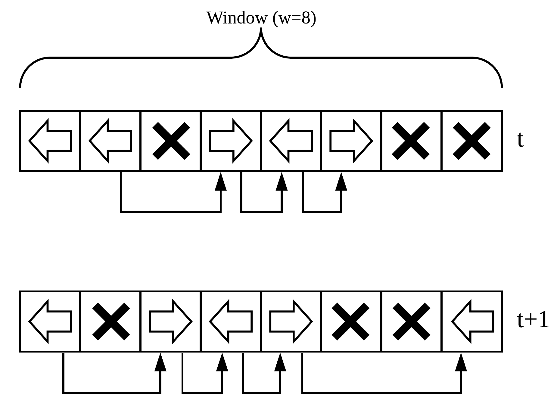
(a) shaking cost

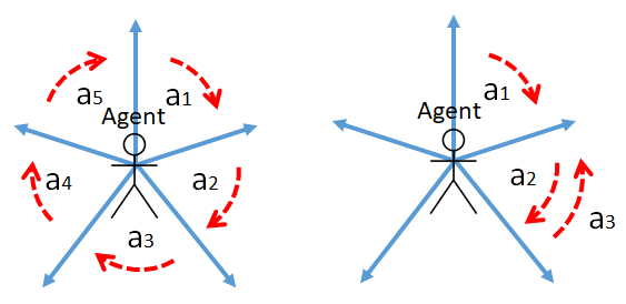
(b) spinning cost

Figure 1: Shaking and spinning costs

First, consider the shaking cost. In 3D games, the shaking behavior of an agent is usually recognized from the quick vibratory movements along a horizontal axis within a short period of time. In many games, shaking is an effective way for computer agents to search target, however, human players tend not to shake too often due to physical fatigue. In this paper, we quantify the amount of shaking as the number of changes in direction within a sliding time window of a fixed size $w\in\mathbb{N}$. Specifically, the shaking cost $C_{sh}(t)$ at time $t$ is defined as follows. For simplicity, let horizontal actions include the three kinds of actions, move-left, move-right, and no operation (no-op). For a sequence of consecutive actions $<a_{i},...,a_{j}>$, if both $a_{i}$ and $a_{j}$ are opposite actions, namely move-left versus move-right, and all actions between the two are no-op, then count one for shaking. In a sequence of $w$ horizontal actions $<a_{t-w+1},...,a_{t}>$, the shaking cost $C_{sh}(t)$ is the total count divided by $w-1$ for normalization. Note that $w-1$ is the maximum count for shaking in a window. As illustrated by an example in Figure 1 (a), the shaking cost for the upper window of size $8$ is $3/7$, and that for the lower window is $4/7$.

Second, consider the spinning cost. In 3D games, shaking is also an effective way for computer agents to search target, and human players tend not to spin too often also due to physical fatigue. In this paper, we quantify the amount of spinning as the number of turning around and back to the original orientation. Specifically, the spinning cost $C_{sh}(t)$ at time $t$ is defined as follows. Count one for spinning whenever the agent turns one whole around, either left or right, and then face to the same orientation. As illustrated by an example in Figure 1 (b), the spinning cost is one for the left with the five actions $<a_{1},...,a_{5}>$, and nothing for the right. Note that for the left we count one more if the next five actions are the same as $<a_{1},...,a_{5}>$.

4 Experiments

Our experiments are run for a game on the ML-Agents Toolkit, called Banana Collector and some of the games on DMLab-30, described in Subsections 4.1 and 4.2 respectively.

4.1 ML-Agents Toolkit Experiment

Our version of ML-Agents Toolkit is 0.8.1. In the game of Banana Collector, the goal of the agent is to get as many yellow bananas (each with reward +1) as possible, while avoiding touching blue bananas (each with reward -1). The game is in a square area, and is ended after the agent takes 2000 steps. To make the area always exist some bananas, bananas will be refilled to the game periodically. For simplicity, the action space only includes the actions of moving and rotating. Other details are listed in Table 1.

Table 1: Environment settings

Statement	Description
Input	160x90 RGB image
Reward	yellow banana: +1
	blue banana: -1
Action	moving: forward, backward, none
	rotating: left, right, none
Game setting	Game steps: 2000
	Total agents: 4
	FPS: 50
	Frame skip: 4

The ML-Agents Toolkit supports Proximal Policy Optimization (PPO) (Schulman et al., 2017) as a default implementation of the learning algorithm, which serves as the baseline agent (without behavioral costs) in this experiment. As this PPO version is implemented with a clipped surrogate objective version, it also enforces the proximity constraint Equation 13. With behavioral costs, we train three agents, named ABC-RL, AB-CPO, and Const, based on Algorithm 1 with the PPO implementation for update and with three different settings for the behavioral weight $\Lambda$ respectively. The agent named ABC-RL uses the same behavioral weight as in Algorithm 1, AB-CPO lets the weight $\Lambda$ follow the formula in Equation 14, and Const fixes $\Lambda$ to constant 1. The behavioral costs follow the formula in Equation 20, but let $\alpha=1$ for simplicity. Namely, $C(t)=C_{sh}(t)+C_{sp}(t)$. The window size for shaking costs is all set to be 8, i.e., $w=8$. Each experiment is run three times with one million steps each.

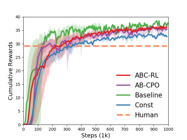
(a) Cumulative rewards

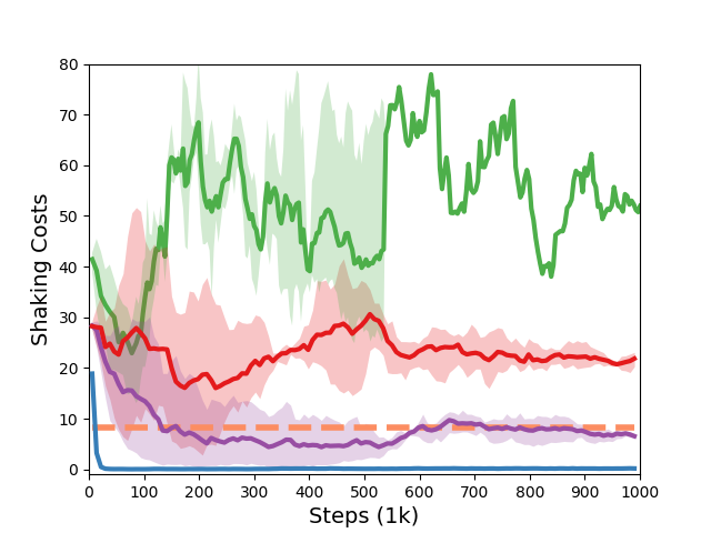
(b) Shaking costs (c) Spinning costs

Figure 2: Results in ML-Agents Toolkit with training steps

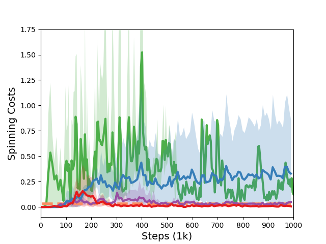
The performances of the above four agents are shown in Figure 2, including cumulative rewards, shaking costs, and spinning costs, where each curve presents the average value of three runs. Without considering behavioral costs, the baseline performs the best for the cumulative rewards, while both shaking and spinning costs are apparently higher than others in most cases. With constant behavioral weight, the agent Const performs the worst clearly, while its shaking costs are the lowest among all agents and its spinning costs are apparently higher than ABC-RL and AB-CPO but comparable to the baseline near the end of the training. The reason for the nearly zero shaking costs under Const is that the value of the shaking cost dominates the objective. Thus, the agent Const learns to prioritize shaking costs, while compromising on spinning costs. Both ABC-RL and AB-CPO perform nearly equally, and near the level of the baseline, though slightly worse. While its performance is retained, both shaking and spinning costs are greatly reduced with respect to the baseline. The spinning costs for both ABC-RL and AB-CPO are very close to 0, much lower than Const. For shaking costs, AB-CPO has a lower curve than ABC-RL.

For comparison to human players, we also record 80 games in total played by 8 human players. The experimental results are shown as horizontal dashed lines in Figure 2. The result shows that all the four agents perform better than human players and that the shaking costs of AB-CPO are comparable to human players, and the spinning costs of both ABC-RL and AB-CPO are close to zero, nearly the same as human players. This also shows that human players tend not to spin. Thus, the comparison shows that both ABC-RL and AB-CPO, particularly for AB-CPO, are able to retain a similar performance while behaving like humans in the aspects of shaking and spinning.

4.2 DMLab-30 Experiments

rooms_keys_doors_puzzle

return

shaking cost

spinning cost

rooms_collect_good_objects_train

return

shaking cost

spinning cost

lasertag_three_opponents_small

return

shaking cost

spinning cost

rooms_watermaze

return

shaking cost

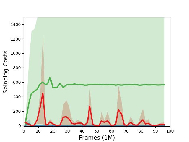
spinning cost

Figure 3: Results in DMLab-30 with training steps

DMLab-30, provided by DeepMind Lab, is a collection of game environments for DRL research in first-person 3D world space. In our study, we conducted experiments on four specific games from DMLab-30 as following:

1. rooms_collect_good_objects: In this game, the agent’s objective is to collect good objects while avoiding bad objects. This game is similar to the Banana Collector game in the ML-Agents Toolkit.

2. rooms_keys_doors_puzzle: This game presents a procedural planning puzzle. The agent must navigate through a series of colored doors that block access to the goal object. The agent is able to keep only one single-use colored key to open the corresponding colored door. The challenge lies in determining the correct sequence of collecting keys and traversing rooms to reach the goal.

3. rooms_watermaze: In this game, the agent’s objective is to locate a hidden platform. Whenever the platform is discovered, the environment generates a reward for the agent and reset the agent’s position. Finding the platform is challenging in initial trails, but the agent should remember its location in subsequent trials and navigate directly to it.

4. lasertag_three_opponents_small: In this game, the agent plays laser tag with other three opponent bots in a small map. The environment contains gadgets and power-ups, which are randomly generated.

These games provide diverse challenges and serve as a testbed for evaluating whether our proposed metrics and the training approach could be a general solution to the problem of creating human-like agents.

For DMLab-30, our experiments are based on the framework SEED RL. As SEED RL supports the implementation of v-trace, but not PPO, the version of V-trace serves as the baseline (without behavioral cost). With behavioral costs, both agents, ABC-RL and Const, are trained in the same way as those in Section 4.1. Note that the proximity constraint Equation 13 is not supported in V-trace. So, we do not implement the agent AB-CPO for fairness of comparison mainly to the baseline, because ABC-RL is also representative as shown in the previous subsection. We run each experiment three times, each with around 100 million frames.

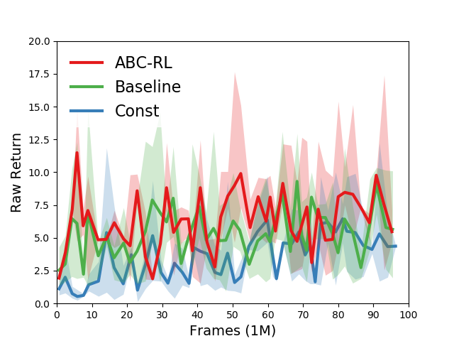
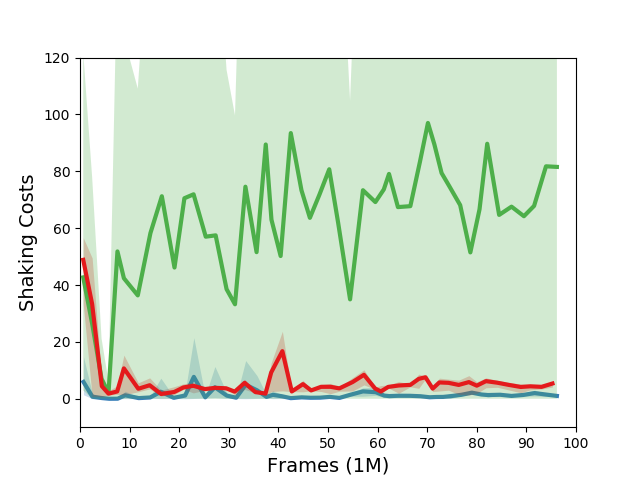
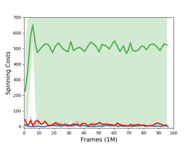
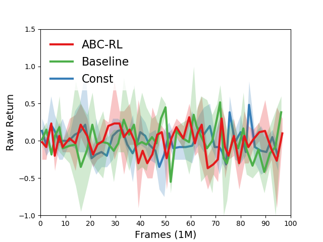
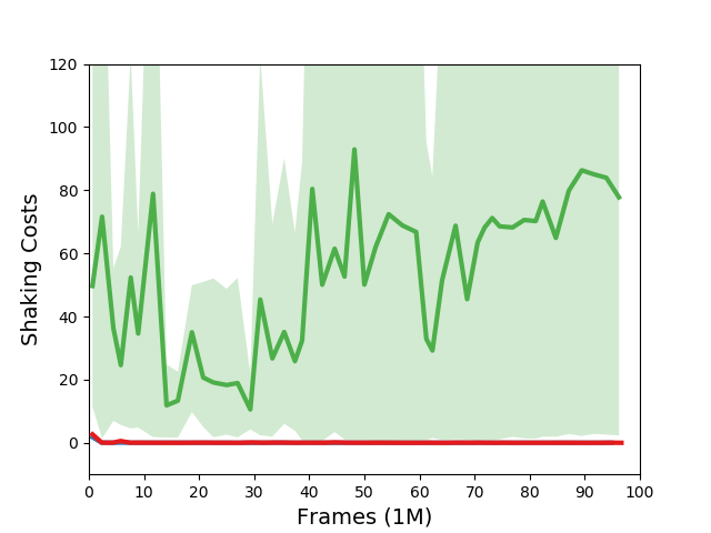
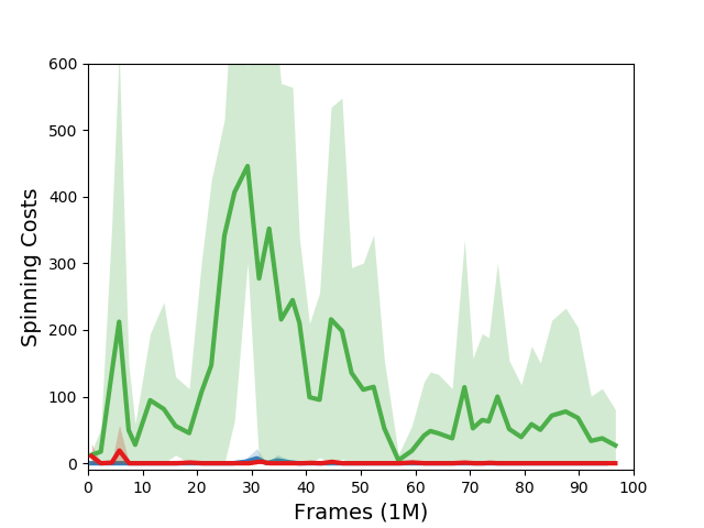
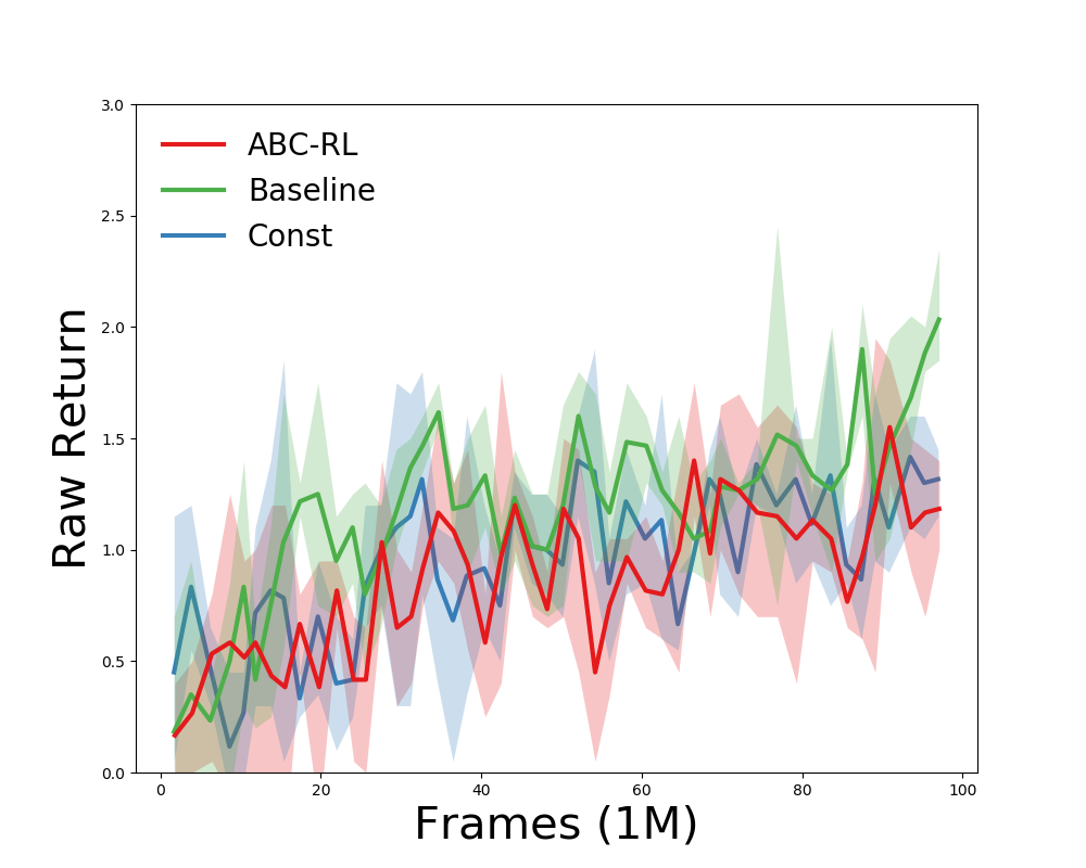
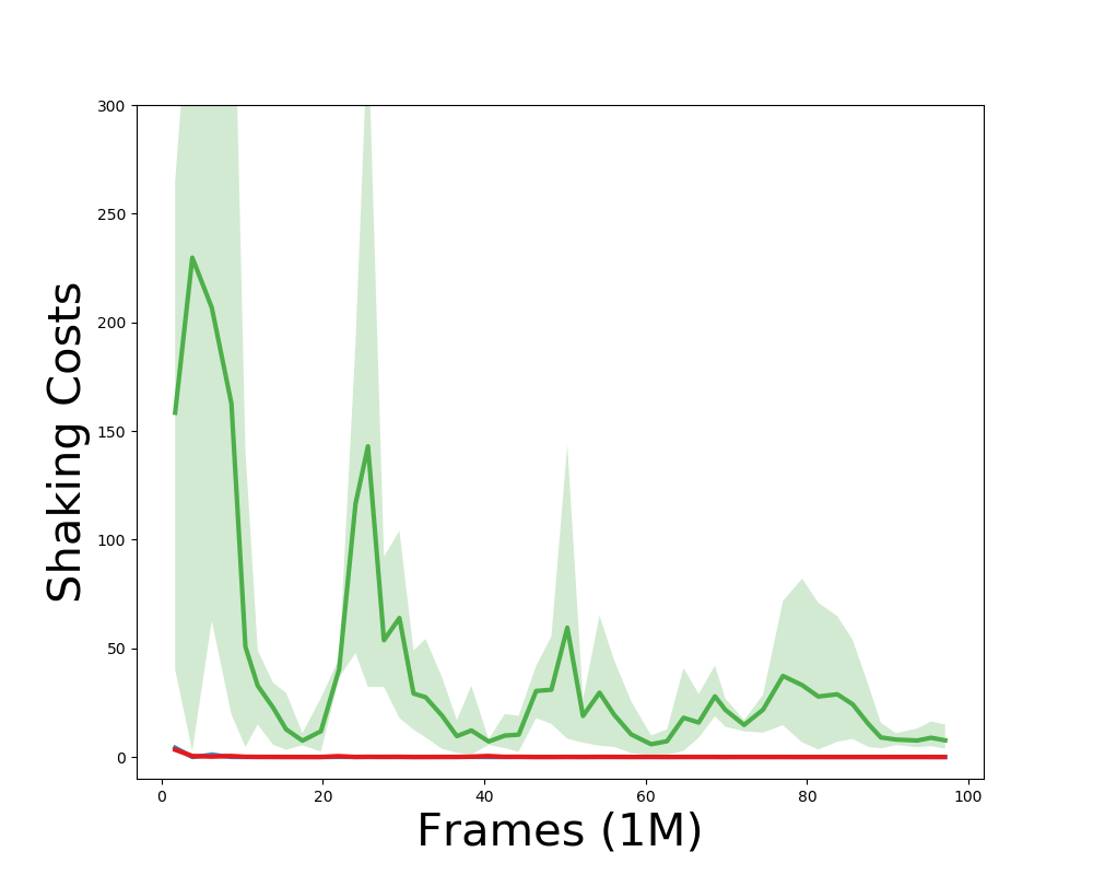
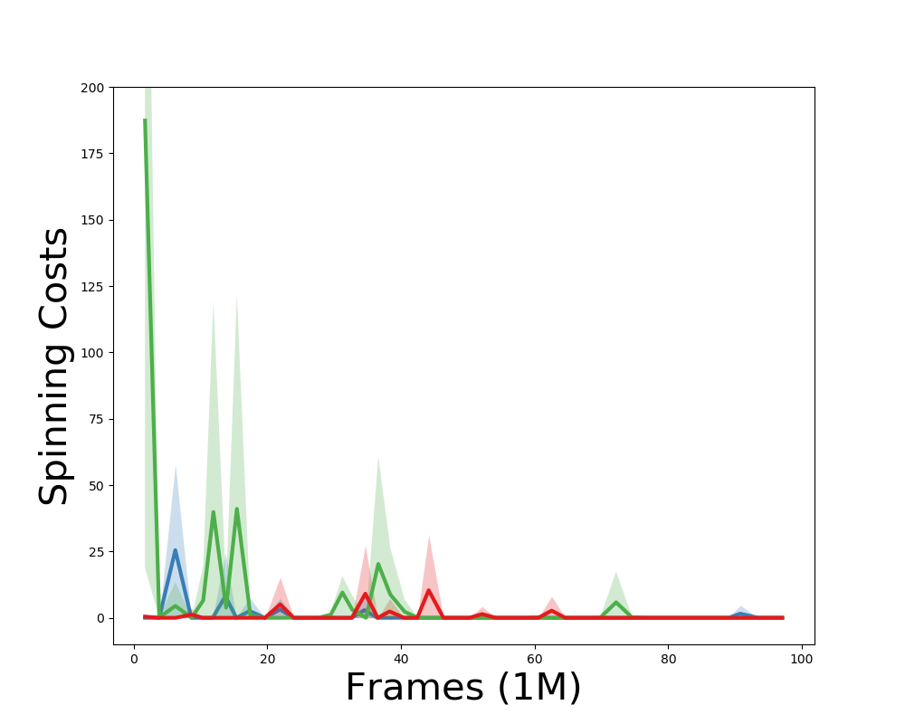
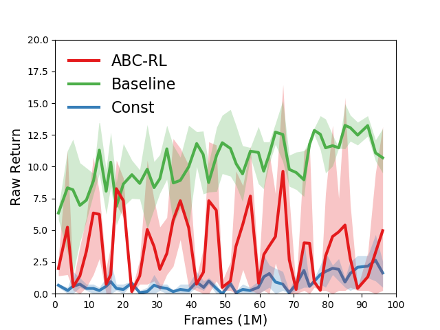
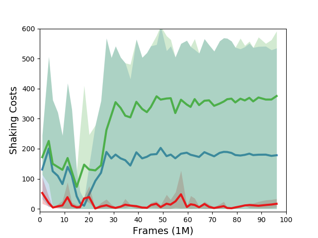
Figure 3 shows the performances of the three agents, ABC-RL, baseline and Const, for the four games respectively. For the game, rooms_keys_doors_puzzle, the performance of ABC-RL is comparable to the baseline, while both shaking and spinning costs are nearly zero, much lower than the baseline. It is similar for the game, rooms_collect_good_objects. For lasertag_three_opponents_small, all methods are steadily improving in raw returns, but different in shaking and spinning costs. ABC-RL and Const obtain near zero about shaking and spinining costs because they consider behavior costs. Baseline shakes and spins a lot in the beginning, but after training, there is a slight amount of shaking and spinning left. For the game, rooms_watermaze, ABC-RL performs better than Const and worse than the baseline, while both shaking and spinning costs are also nearly zero, much lower than the baseline. However, it is interesting to observe the fluctuation of the performance of ABC-RL. Since agents in this game need to a find hidden platform for rewards, it is critical to take shaking and spinning actions. Once the agent ABC-RL receives high rewards, the behavioral weight grows, and hence it discourages the actions of shaking and spinning. In such a situation, it becomes hard to find platforms and therefore the subsequent performance is reduced. The phenomenon illustrates the case that the behavioral costs are highly correlated to the performance increase. Whether there is a way of defining the cost to prevent this case is not in the scope of this paper.

5 Conclusion

The contribution of this paper is summarized as follows. First, we propose a new approach called Adaptive Behavioral Costs in Reinforcement Learning (ABC-RL) for training a human-like agent with competitive strength. To behave like humans and retain similar performance, ABC-RL augments behavioral limitations as cost signals in reinforcement learning with dynamically adjusted weights. Second, for ABC-RL, we propose a novel formulation that minimizes the behavioral costs subject to a constraint of the value function. By leveraging the augmented Lagrangian, our approach is an approximation of the Lagrangian adjustment, which handles the trade-off between the performance and the human-like behavior. Although this paper presents behavioral costs based on shaking and spinning, we leave the definition of the costs open, e.g., different $\alpha$ or other non-human-like actions. Third, in the 3D games of DMLab-30 and Unity ML-Agents Toolkit, our experiments show that ABC-RL preserves nearly the same performance level with significantly less shaking and spinning, as shown in Figures 2 and 3.

References

- Abad and Krishnamurthy (2003) Felisa Vázquez Abad and Vikram Krishnamurthy. Self learning control of constrained markov decision processes - a gradient approach. In IEEE Conference on Decision and Control (CDC), 2003.
- Achiam et al. (2017) Joshua Achiam, David Held, Aviv Tamar, and Pieter Abbeel. Constrained policy optimization. In International Conference on Machine Learning (ICML), 2017.
- Altman (1996) Eitan Altman. Constrained markov decision processes with total cost criteria: Occupation measures and primal LP. Mathematical Methods of Operations Research, 1996.
- Badia et al. (2020) Adrià Puigdomènech Badia, Bilal Piot, Steven Kapturowski, Pablo Sprechmann, Alex Vitvitskyi, Zhaohan Daniel Guo, and Charles Blundell. Agent57: Outperforming the atari human benchmark. In International Conference on Machine Learning (ICML), 2020.
- Beattie et al. (2016) Charles Beattie, Joel Z. Leibo, Denis Teplyashin, Tom Ward, Marcus Wainwright, Heinrich Küttler, Andrew Lefrancq, Simon Green, Víctor Valdés, Amir Sadik, Julian Schrittwieser, Keith Anderson, Sarah York, Max Cant, Adam Cain, Adrian Bolton, Stephen Gaffney, Helen King, Demis Hassabis, Shane Legg, and Stig Petersen. Deepmind lab. CoRR, abs/1612.03801, 2016.
- Berner et al. (2019) Christopher Berner, Greg Brockman, Brooke Chan, Vicki Cheung, Przemyslaw Debiak, Christy Dennison, David Farhi, Quirin Fischer, Shariq Hashme, Christopher Hesse, Rafal Józefowicz, Scott Gray, Catherine Olsson, Jakub Pachocki, Michael Petrov, Henrique Pondé de Oliveira Pinto, Jonathan Raiman, Tim Salimans, Jeremy Schlatter, Jonas Schneider, Szymon Sidor, Ilya Sutskever, Jie Tang, Filip Wolski, and Susan Zhang. Dota 2 with large scale deep reinforcement learning. CoRR, abs/1912.06680, 2019.
- Bertsekas (1999) Dimitri P Bertsekas. Nonlinear programming. Athena Scientific, 1999.
- Borkar (2005) Vivek S. Borkar. An actor-critic algorithm for constrained markov decision processes. Systems and Control Letters, 2005.
- Chow et al. (2017) Yinlam Chow, Mohammad Ghavamzadeh, Lucas Janson, and Marco Pavone. Risk-constrained reinforcement learning with percentile risk criteria. Journal of Machine Learning Research (JMLR), 2017.
- de Woillemont et al. (2022) Pierre Le Pelletier de Woillemont, Rémi Labory, and Vincent Corruble. Automated play-testing through RL based human-like play-styles generation. In Stephen G. Ware and Markus Eger, editors, Artificial Intelligence and Interactive Digital Entertainment (AIIDE), 2022.
- Devlin et al. (2021) Sam Devlin, Raluca Georgescu, Ida Momennejad, Jaroslaw Rzepecki, Evelyn Zuniga, Gavin Costello, Guy Leroy, Ali Shaw, and Katja Hofmann. Navigation turing test (NTT): learning to evaluate human-like navigation. In Marina Meila and Tong Zhang, editors, International Conference on Machine Learning (ICML), 2021.
- Emuna et al. (2020) Ran Emuna, Avinoam Borowsky, and Armin Biess. Deep reinforcement learning for human-like driving policies in collision avoidance tasks of self-driving cars. CoRR, abs/2006.04218, 2020.
- Fujii et al. (2013) Nobuto Fujii, Yuichi Sato, Hironori Wakama, Koji Kazai, and Haruhiro Katayose. Evaluating human-like behaviors of video-game agents autonomously acquired with biological constraints. In Advances in Computer Entertainment (ACE), 2013.
- García and Fernández (2015) Javier García and Fernando Fernández. A comprehensive survey on safe reinforcement learning. Journal of Machine Learning Research (JMLR), 2015.
- Garg et al. (2023) Divyansh Garg, Joey Hejna, Matthieu Geist, and Stefano Ermon. Extreme q-learning: Maxent RL without entropy. In International Conference on Learning Representations (ICLR), 2023.
- Ho and Ermon (2016) Jonathan Ho and Stefano Ermon. Generative adversarial imitation learning. In Advances in Neural Information Processing Systems (NIPS), 2016.
- Horgan et al. (2018) Dan Horgan, John Quan, David Budden, Gabriel Barth-Maron, Matteo Hessel, Hado van Hasselt, and David Silver. Distributed prioritized experience replay. In International Conference on Learning Representations, (ICLR), 2018.
- Jacob et al. (2022) Athul Paul Jacob, David J. Wu, Gabriele Farina, Adam Lerer, Hengyuan Hu, Anton Bakhtin, Jacob Andreas, and Noam Brown. Modeling strong and human-like gameplay with kl-regularized search. In International Conference on Machine Learning (ICML), 2022.
- Jaderberg et al. (2019) Max Jaderberg, Wojciech Czarnecki, Iain Dunning, Luke Marris, Guy Lever, Antonio García Castañeda, Charles Beattie, Neil C. Rabinowitz, Ari S. Morcos, Avraham Ruderman, Nicolas Sonnerat, Tim Green, Louise Deason, Joel Z. Leibo, David Silver, Demis Hassabis, Koray Kavukcuoglu, and Thore Graepel. Human-level performance in 3d multiplayer games with population-based reinforcement learning. Science, 2019.
- Juliani et al. (2018) Arthur Juliani, Vincent-Pierre Berges, Esh Vckay, Yuan Gao, Hunter Henry, Marwan Mattar, and Danny Lange. Unity: A general platform for intelligent agents. CoRR, abs/1809.02627, 2018.
- Kapturowski et al. (2019) Steven Kapturowski, Georg Ostrovski, John Quan, Rémi Munos, and Will Dabney. Recurrent experience replay in distributed reinforcement learning. In International Conference on Learning Representations, (ICLR), 2019.
- Kumar et al. (2020) Aviral Kumar, Aurick Zhou, George Tucker, and Sergey Levine. Conservative q-learning for offline reinforcement learning. In Hugo Larochelle, Marc’Aurelio Ranzato, Raia Hadsell, Maria-Florina Balcan, and Hsuan-Tien Lin, editors, Advances in Neural Information Processing Systems (NeurIPS), 2020.
- Liu et al. (2019) Yongshuai Liu, Jiaxin Ding, and Xin Liu. IPO: interior-point policy optimization under constraints. CoRR, abs/1910.09615, 2019.
- Milani et al. (2023) Stephanie Milani, Arthur Juliani, Ida Momennejad, Raluca Georgescu, Jaroslaw Rzepecki, Alison Shaw, Gavin Costello, Fei Fang, Sam Devlin, and Katja Hofmann. Navigates like me: Understanding how people evaluate human-like AI in video games. In International Conference on Human Factors in Computing Systems (CHI), 2023.
- Mnih et al. (2015) Volodymyr Mnih, Koray Kavukcuoglu, David Silver, Andrei A. Rusu, Joel Veness, Marc G. Bellemare, Alex Graves, Martin A. Riedmiller, Andreas K. Fidjeland, Georg Ostrovski, Stig Petersen, Charles Beattie, Amir Sadik, Ioannis Antonoglou, Helen. King, Dharshan Kumaran, Daan Wierstra, Shane Legg, and Demis Hassabis. Human-level control through deep reinforcement learning. Nature, 2015.
- Mnih et al. (2016) Volodymyr Mnih, Adrià Puigdomènech Badia, Mehdi Mirza, Alex Graves, Timothy P. Lillicrap, Tim Harley, David Silver, and Koray Kavukcuoglu. Asynchronous methods for deep reinforcement learning. In International Conference on Machine Learning (ICML), 2016.
- Momennejad (2023) Ida Momennejad. A rubric for human-like agents and neuroai. Philosophical Transactions of the Royal Society B, 2023.
- Najar and Chetouani (2021) Anis Najar and Mohamed Chetouani. Reinforcement learning with human advice: A survey. Frontiers in Robotics and AI, 2021.
- Rosenfeld et al. (2018) Ariel Rosenfeld, Moshe Cohen, Matthew E. Taylor, and Sarit Kraus. Leveraging human knowledge in tabular reinforcement learning: a study of human subjects. The knowledge engineering review, 2018.
- Schulman et al. (2017) John Schulman, Filip Wolski, Prafulla Dhariwal, Alec Radford, and Oleg Klimov. Proximal policy optimization algorithms. CoRR, abs/1707.06347, 2017.
- Sutton and Barto (2018) Richard S Sutton and Andrew G Barto. Reinforcement learning: An introduction. MIT press, second edition, 2018.
- Tessler et al. (2019) Chen Tessler, Daniel J. Mankowitz, and Shie Mannor. Reward constrained policy optimization. In International Conference on Learning Representations (ICLR), 2019.
- van Hasselt et al. (2016) Hado van Hasselt, Arthur Guez, and David Silver. Deep reinforcement learning with double q-learning. In AAAI Conference on Artificial Intelligence (AAAI), 2016.
- Vinyals et al. (2019a) Oriol Vinyals, Igor Babuschkin, Wojciech M. Czarnecki, Michaël Mathieu, Andrew Dudzik, Junyoung Chung, David H. Choi, Richard Powell, Timo Ewalds, Petko Georgiev, Junhyuk Oh, Dan Horgan, Manuel Kroiss, Ivo Danihelka, Aja Huang, L. Sifre, Trevor Cai, John P. Agapiou, Max Jaderberg, Alexander Sasha Vezhnevets, Rémi Leblond, Tobias Pohlen, Valentin Dalibard, David Budden, Yury Sulsky, James Molloy, Tom Le Paine, Caglar Gulcehre, Ziyun Wang, Tobias Pfaff, Yuhuai Wu, Roman Ring, Dani Yogatama, Dario Wünsch, Katrina McKinney, Oliver Smith, Tom Schaul, Timothy P. Lillicrap, Koray Kavukcuoglu, Demis Hassabis, Chris Apps, and David Silver. Grandmaster level in starcraft ii using multi-agent reinforcement learning. Nature, 2019a.
- Vinyals et al. (2019b) Oriol Vinyals, Igor Babuschkin, Wojciech Marian Czarnecki, Michaël Mathieu, Andrew Joseph Dudzik, Junyoung Chung, Duck Hwan Choi, Richard W. Powell, Timo Ewalds, Petko Georgiev, Junhyuk Oh, Dan Horgan, Manuel Kroiss, Ivo Danihelka, Aja Huang, Laurent Sifre, Trevor Cai, John P. Agapiou, Max Jaderberg, Alexander Sasha Vezhnevets, Rémi Leblond, Tobias Pohlen, Valentin Dalibard, David Budden, Yury Sulsky, James Molloy, Tom Le Paine, Caglar Gulcehre, Ziyu Wang, Tobias Pfaff, Yuhuai Wu, Roman Ring, Dani Yogatama, Dario Wünsch, Katrina McKinney, Oliver Smith, Tom Schaul, Timothy P. Lillicrap, Koray Kavukcuoglu, Demis Hassabis, Chris Apps, and David Silver. Grandmaster level in starcraft ii using multi-agent reinforcement learning. Nature, 2019b.
- Wang et al. (2016) Ziyu Wang, Tom Schaul, Matteo Hessel, Hado van Hasselt, Marc Lanctot, and Nando de Freitas. Dueling network architectures for deep reinforcement learning. In International Conference on Machine Learning, (ICML), 2016.
- Yang et al. (2020) Tsung-Yen Yang, Justinian Rosca, Karthik Narasimhan, and Peter J. Ramadge. Projection-based constrained policy optimization. In International Conference on Learning Representations (ICLR), 2020.
- Zhu et al. (2019) Meixin Zhu, Xuesong Wang, and Yinhai Wang. Human-like autonomous car-following model with deep reinforcement learning. CoRR, abs/1901.00569, 2019.
- Zuniga et al. (2022) Evelyn Zuniga, Stephanie Milani, Guy Leroy, Jaroslaw Rzepecki, Raluca Georgescu, Ida Momennejad, David Bignell, Mingfei Sun, Alison Shaw, Gavin Costello, Mikhail Jacob, Sam Devlin, and Katja Hofmann. How humans perceive human-like behavior in video game navigation. In International Conference on Human Factors in Computing Systems (CHI) Extended Abstracts, 2022.