Prosumers Participation in Markets:
A Scalar-Parameterized Function Bidding Approach

Abstract

In uniform-price markets, suppliers compete to supply a resource to consumers, resulting in a single market price determined by their competition. For sufficient flexibility, producers and consumers prefer to commit to a function as their strategies, indicating their preferred quantity at any given market price. Producers and consumers may wish to act as both, i.e., prosumers. In this paper, we examine the behavior of profit-maximizing prosumers in a uniform-price market for resource allocation with the objective of maximizing the social welfare. We propose a scalar-parameterized function bidding mechanism for the prosumers, in which we establish the existence and uniqueness of Nash equilibrium. Furthermore, we provide an efficient way to compute the Nash equilibrium through the computation of the market allocation at the Nash equilibrium. Finally, we present a case study to illustrate the welfare loss under different variations of market parameters, such as the market’s supply capacity and inelastic demand.

I Introduction

The competition for a divisible resource between selfish agents has made game-theoretic methods useful tools for the design of resource allocation mechanisms. For such mechanisms design, several metrics have been investigated in the literature, such as fairness and social welfare efficiency of the allocation as well as the computational cost for finding the allocation where strategy space plays a significant role. One measure of fairness was discussed in [1] for a proportionally fair (PF) pricing mechanism where the resulting allocation makes it impossible to increase the sum of weighted proportional gains. Another design metric is the efficiency of allocation with respect to social welfare maximization, i.e., to what extent the sum of agents’ utilities is close to the maximum possible value. Efficiency of the aforementioned PF pricing mechanism, however, is undermined when agents behave strategically, i.e., when their strategies incorporate the relationship of the price to the bids—this turns the mechanism into an auction. In a competitive formulation, [2] studied the efficiency loss of this PF auction and showed that it is 25% in the worst case.

Vickrey-Clarke-Groves (VCG) is a well-known class of mechanisms [3, 4, 5] for resource allocation which ensures that truthful reporting of each agent is a dominant strategy. However, it may not be practical for some domains because of shortcomings such as providing a different price to different agents for the same resource. Other mechanisms similar to VCG were studied for pricing divisible resources with scalar strategy spaces such as [6, 7]; see section 2 of [8] for an extended list. [6] investigated a PF divisible auction in which the notions of price and demand functions were introduced to characterize optimal response functions of the agents. A unique Nash equilibrium was proven to exist for agents with heterogeneous quasilinear utilities and a decentralized iterative algorithm was described to converge to the equilibrium. A class of mechanisms with single-dimensional signaling (bidding strategy) was studied in [7] where the PF auction was shown to be inefficient in general. An infinite subclass of efficient signal proportional allocation (ESPA) mechanisms was shown to maximize the social welfare for agents with quasi-linear utilities. Besides efficiency, computational cost and signaling space are other design metrics in which ESPA is an optimal allocation mechanism.

The analysis of supply function equilibria (SFE) for uniform-price markets is closely related to this growing literature on efficiency guarantees in market design. In such bidding mechanisms and for sufficient flexibility, competing suppliers prefer to commit to (offer) supply functions as their strategies, indicating their preferred supply quantity at any given market price. This is in contrast to committing to a scalar strategy, such as a fixed price (Bertrand model) or a fixed quantity (Cournot model). [9] investigated the existence of Nash equilibria resulting from supply function bids, more precisely supply offers, and demonstrated that they can be highly inefficient.

In a centralized uniform-price market-clearing mechanism for supply-quantity allocation of an infinitely divisible resource, [8] proposed a restriction on the class of supply functions, limiting the supplier’s strategy to scalar-parameterized functions. Under a fixed, inflexible (inelastic) demand and suppliers with maximum production capacity, the paper studied the existence of Nash equilibrium and the efficiency of its associated market allocation. This formulation was extended in [10] to study capacity constrained suppliers and inelastic demands that are spread throughout a transmission constrained power network. By studying the efficiency of Nash equilibrium’s market allocation, the paper explained how certain market structures, such as market share and residual supply index, can be useful in predicting the extent to which each supplier can exert market power to influence the market outcome to its advantage. In [11], the assumption of total inelastic demand in [8] was relaxed to study two-sided markets (producers and consumers) with multiple strategic consumers having both elastic (flexible) and inelastic (minimum) demands, where the strategies of both producers and consumers are scalar-parameterized functions. In some markets, the distinction between producers and consumers may not be needed such that the participants may wish to act as both. These participants are often called prosumers. This paper proposes a scalar-parameterized function for the prosumer markets.

Given that electricity is a prime example of an infinitely divisible resource with ample research on its prosumer markets, the remaining part of this introduction reviews the literature on the participation of prosumers in electricity markets. Different structures for prosumer electricity markets were discussed in [12]. From game-theoretic point of view, these structures can be classified into three main typologies: peer-to-peer model in which competitive prosumers interact directly with each other within a region (neighborhood), prosumer-to-microgrids model in which competitive prosumers interact under a central microgrid-operator which also interacts with other neighbor microgrid-operators, and organized-prosumer-group model in which a group of prosumers cooperate to form a virtual power plant which is connected to the main grid.

Prosumers, as individual agents involved in distributed decision making, are closely related to other similar agents discussed in the electricity markets literature such as interconnected microgrids and controllable loads [13]. The aforementioned scalar-parameterized supply functions were reformulated in [14] such that they are used as bidding mechanism for the consumers who are equipped with controllable loads. The paper studied the existence of Nash equilibrium and the efficiency of its associated allocation of the consumers’ load adjustment capacities. Prosumers and interconnected microgrids, however, differ from controllable demand in their objective functions, as they are agents equipped (directly or by proxy) with production capability that comes with an associated cost. Given the various possible structures in which these competitive or cooperative agents can participate in electricity markets, game-theoretic methods are attractive tools for such applications due to their effectiveness in analyzing multi-agent strategic decision making.

In non-cooperative settings, whether the typology of prosumers is peer-to-peer or prosumer-to-microgrids, there are several solution concepts in game theory that are useful for analyzing such typologies [13]. For example, Nash equilibrium is suitable for non-cooperative games where no player dominates the decision process whereas Stackelberg equilibrium is useful when hierarchy is allowed in the decision process [15].

Compared to a large producer in the wholesale electricity market (within the main grid), the size of a prosumer is often too small to participate in such a market. Hence, retail aggregators offer a reasonable solution to enable the participation of prosumers in the wholesale market. In this trading setting where a profit-maximizing retail agreggator sets a uniform price for its competitive prosumers, [16] formulated a Stackelberg game between the aggregator and the prosumers and characterized the Stackelberg equilibrium. The goal was to quantify the loss in efficiency (e.g. welfare loss) that may result from the strategic incentive of the aggregator, when compared to the benchmark efficiency in which the prosumers directly participate in the wholesale market. [17] introduced a framework where an aggregator incentivizes its prosumers to produce or consume energy over a period of time by setting two prices: one for production and another for consumption. The paper focuses on the prosumer’s strategic decision-making process which was formulated as a game with the aggregator. For such a game, sufficient conditions on the aggregator’s pricing strategy were established for the existence of a unique Nash equilibrium. Also, a distributed algorithm was proposed which enables the prosumers to seek this Nash equilibrium, relying on local information acquired through exchange of information with neighboring prosumers. Furthermore, the algorithm was proven to be asymptotically convergent, when the network of prosumers is connected and undirected.

Among the several typologies above for the prosumer markets, this paper restricts the analysis on a peer-to-peer model. We generally seek to have an efficient Nash equilibrium in the design of uniform-price market where strategic (price-anticipating) market participants compete for an infinitely divisible resource. In other words, we want the market’s aggregate cost at the Nash equilibrium to be close to the minimum possible cost (i.e. the socially-optimal cost or cost at the price-taking competitive equilibrium). Equivalently, we seek to have a social welfare at the Nash equilibrium that is close to the socially-optimal welfare. Our goal is to study the market design question of how to formulate a bidding mechanism that provides sufficient flexibility for the prosumers to declare their bidding preferences in a way that yields an efficient allocation of productions and consumptions, minimizing the “welfare loss” that occurs due to their strategic behavior. In other words, are there any restrictions that can be placed on the declared bidding functions to ensure such an efficient allocation?

Due to its ability to simultaneously produce and consume, a prosumer’s consumption volume from other market participants may not be zero even when the net supply is positive (i.e., the prosumer supplies more than it consumes). In this case, the prosumer still has consumption utility and cost. This feature is known as prosumer duality. By expanding the traditional Cournot model, [18] demonstrated by simulations that the dual nature of prosumers can lead to more competitive behavior than pure producers in a traditional producer/consumer system. In other words, the prosumers’ best-response supply quantities are closer to the competitive levels than those of the traditional producers, under the same game-theoretic scenario. The design that we propose considers the net quantity of supply/demand but does not consider the prosumer’s duality; which is recommended for future research.

The rest of the paper is organized as follows: Section II introduces the bidding mechanism for the prosumers and the market model (optimization of resource allocation) for the central clearinghouse. Section III discusses the competitive equilibrium where the prosumers are price-takers. Section IV investigates the Nash equilibrium where the prosumers are price-makers (strategic). Section V outlines a case study where the market outcome (allocation) is examined with respect to the welfare loss when different market parameters (e.g. supply capacity or inelastic demand) are varied. Section VI concludes and provides future directions.

II Bidding Mechanism and Market Model

To investigate the posed market design question, we consider profit maximizing prosumers having production costs and utilities characterized, respectively, by convex cost functions and concave utility functions in the output quantity. Each prosumer has a maximum production capacity and a minimum inelastic demand. In the search for a restriction on general bidding functions to scalar-parameterized ones, analogous to [8] for one-sided market of suppliers and [11] for two-sided market of suppliers and consumers, it is natural to first examine the possibility of using the supply offers and demand bids proposed in [11] so that together they represent the prosumer’s strategy—using this bidding mechanism enables the dual nature of prosumers. Denote the set of prosumers by $\mathcal{N}$=$\{1,2,\ldots,N\}$. Let $d_{min}\in\mathbb{R}^{+}$ represent the minimum inelastic (inflexible) demand for each prosumer, and $s_{max}\in\mathbb{R}^{+}$ denote the maximum supply capacity. Their values are assumed to be identical for all prosumers without loss of generality. In the paper, we emphasize the distinction between the supply capacity $s_{max}$ and the production capacity. The production capacity includes not only the supply capacity but also the capacity used by each prosumer to meet its own demand, i.e., the production capacity is $s_{max}+d_{min}$. In addition, $\theta_{i}^{s}\in\mathbb{R}^{+}$ and $\theta_{i}^{d}\in\mathbb{R}^{+}$ are the parameters to be chosen by prosumer $i$ to declare its preferred quantity of supply and demand, respectively. Also, $p\in\mathbb{R}^{+}$ is the price to be determined by the market operator (central clearinghouse) to clear the market. The bidding functions are:

$$\begin{split}&s_{i}=S(\theta_{i}^{s},p)\coloneqq s_{max}-\frac{\theta_{i}^{s}}{p},\ \text{and}\\ &d_{i}=D(\theta_{i}^{d},p)\coloneqq d_{min}+\frac{\theta_{i}^{d}}{p},\ i\in\mathcal{N}\vspace{-5pt}\end{split}$$ (1)

Furthermore, each prosumer has a production cost function $C_{i}(s_{i})$ that is continuously differentiable, convex, and increasing as well as a utility function $U_{i}(d_{i})$ that is continuously differentiable, concave, and increasing. In a perfect competition setting where the prosumers are price takers, given a market price $\mu{>}0$ each prosumer maximizes a payoff function given by:

$$\begin{split}\pi_{i}^{p}(\theta_{i}^{d},\theta_{i}^{s},\mu)=&U_{i}(D(\theta_{i}^{d},\mu))-\mu D(\theta_{i}^{d},\mu)\\ &+\mu S(\theta_{i}^{s},\mu)-C_{i}(S(\theta_{i}^{s},\mu))\end{split}$$ (2)

The market operator chooses the price $p(\bm{\theta}^{d},\bm{\theta}^{s})>0$ to clear the market, i.e., so that the supply/demand balance equation $\sum_{i=1}^{N}D(\theta_{i}^{d},p(\bm{\theta}^{d},\bm{\theta}^{s}))=\sum_{i=1}^{N}S(\theta_{i}^{s},p(\bm{\theta}^{d},\bm{\theta}^{s}))$ is satisfied in which case:

$$p(\bm{\theta}^{d},\bm{\theta}^{s})=\frac{\sum_{i=1}^{N}(\theta_{i}^{d}+\theta_{i}^{s})}{N(s_{max}-d_{min})}$$ (3)

In an oligopoly setting where the prosumers are price-anticipating, each prosumer maximizes the following payoff function which is similar to (2) except that now the prosumer realizes that the price is set as a function of all prosumers’ actions according to (3), i.e., $\mu=p(\bm{\theta}^{d},\bm{\theta}^{s})$. Consequently, this incentivizes the prosumers to strategically adjust their payoffs to gain more profits.

$$\begin{split}\pi_{i}^{p}(\theta_{i}^{d},\theta_{-i}^{d},\theta_{i}^{s},\theta_{-i}^{s})=&U_{i}(D(\theta_{i}^{d},p(\bm{\theta}^{d},\bm{\theta}^{s})))-p(\bm{\theta}^{d},\bm{\theta}^{s})\\ &\times D(\theta_{i}^{d},p(\bm{\theta}^{d},\bm{\theta}^{s}))+p(\bm{\theta}^{d},\bm{\theta}^{s})\\ &\times S(\theta_{i}^{s},p(\bm{\theta}^{d},\bm{\theta}^{s}))-C_{i}(S(\theta_{i}^{s},p(\bm{\theta}^{d},\bm{\theta}^{s})))\end{split}$$ (4)

Given the game $\mathcal{G}$ defined by the set of prosumers $\mathcal{N}$, their payoffs given by (4) and their action spaces $\bm{\Theta}_{i}^{d}=\mathbb{R}^{+}$ and $\bm{\Theta}_{i}^{s}=\mathbb{R}^{+}$, a bidding profile $(\bm{\tilde{\theta}}^{d},\bm{\tilde{\theta}}^{s})$ is a Nash equilibrium if:

$$\begin{aligned} &\pi_{i}^{p}(\tilde{\theta}_{i}^{d},\tilde{\theta}_{-i}^{d},\tilde{\theta}_{i}^{s},\tilde{\theta}_{-i}^{s})\geq\pi_{i}^{p}(\theta_{i}^{d},\tilde{\theta}_{-i}^{d},\theta_{i}^{s},\tilde{\theta}_{-i}^{s}),\forall\theta_{i}^{d},\theta_{i}^{s},i\in\mathcal{N}\end{aligned}$$ (5)

Unfortunately, the payoff function (4) increases without a bound since it is not concave in the pair $(\theta_{d}^{i},\theta_{s}^{i})$. Therefore, the problem is not well defined. As a result, we propose an alternative bidding mechanism to (1) for the prosumers. Let $q_{i}\in\mathbb{R}$ denote the desired quantity of demand (positive) or supply (negative) for each prosumer $i$, $d_{min}>0$ be the minimum inelastic demand, $s_{max}>0$ be the maximum supply capacity, and $p>0$ represent the market’s price. We propose the following bidding mechanism which consists of a scalar-parameterized function representing the quantity $q_{i}$ and a scalar representing $s_{max}$:

$$q_{i}=Q(\theta_{i},p)\coloneqq d_{min}+\frac{\theta_{i}}{p},\ \ \text{and}\ s_{max},\ \ i\in\mathcal{N}\vspace{-5pt}$$ (6)

Note that $d_{min}$ is included in the scalar-parameterized function. Also, $q_{i}$ and $s_{max}$ in the bidding mechanism (6) must satisfy $s_{max}\geq-q_{i}$. Prosumer $i$ chooses the parameter $\theta_{i}{\in}\mathbb{R}$ such that $\theta_{i}{>}0$ and $\theta_{i}{\leq}0$ represent, respectively, the pure-consumption and prosumption modes. Thus, $q_{i}{>}d_{min}$ is the pure-consumption mode such that $q_{i}$ is the quantity to be consumed by prosumer $i$ including the inelastic demand $d_{min}$, $q_{i}{<0}$ is the supply mode such that $q_{i}$ is the quantity to be produced by prosumer $i$ including the quantity produced to meet its own inelastic demand $d_{min}$ (local inelastic demand), and $0\leq q_{i}\leq d_{min}$ is the prosumption mode such that $q_{i}$ is the locally unmet portion of the inelastic demand $d_{min}$ to be consumed by prosumer $i$ from other prosumers (hence, $d_{min}-q_{i}$ is prosumer $i$’s produced quantity which is consumed locally). Note that using this bidding mechanism, each prosumer cannot supply to other prosumers until it produces its own entire inelastic demand, i.e., the mechanism does not allow the duality of prosumers. The market operator solves the following convex optimization problem to maximize the aggregate social welfare defined in (7a):

$$\underset{\bm{q}}{\text{maximize}}\ \ \mathcal{W}(\bm{q})\coloneqq\ \ \sum_{i=1}^{N}S_{i}(q_{i}),$$ (7a)

subject to $$\sum_{i=1}^{N}q_{i}=0,$$ (7b)

$$s_{max}\geq-q_{i},\ \forall i\in\mathcal{N}$$ (7c)

where $S_{i}(q_{i})$ is the utility/cost function for prosumer $i$, i.e., utility function when it is positive or cost function when it is negative. Any solution $\bm{q}$ (i.e. allocation profile) to (7) is referred to as an efficient allocation. We impose the following assumption on $S_{i}(q_{i})$:

Assumption 1.

Let $N\geq 2$ and for $\forall i\in\mathcal{N}$, $q_{i},q_{i}^{\prime}\in\mathbb{R}$, $d_{min}>0$, $s_{max}>0$, and $-s_{max}\leq q_{i}<q_{i}^{\prime}$, $S_{i}(q_{i})$ is twice continuously differentiable, strictly increasing, $S_{i}(d_{min})=0$ and satisfies the following condition which is stricter than strict concavity:

$$(1+\frac{q_{i}^{\prime}}{\scalebox{0.9}{\mbox{$\displaystyle(N-1)d_{min}$}}})\frac{\partial S_{i}(q_{i}^{\prime})}{\partial q_{i}^{\prime}}<(1+\frac{q_{i}}{\scalebox{0.9}{\mbox{$\displaystyle(N-1)d_{min}$}}})\frac{\partial S_{i}(q_{i})}{\partial q_{i}}$$ (8)

The market operator chooses the price $p(\bm{\theta})>0$ to clear the market, i.e., so that the supply/demand balance constraint (7b) $\sum_{i=1}^{N}Q(\theta_{i},p(\bm{\theta}))=0$ is satisfied in which case:

$$p(\bm{\theta})=-\frac{\sum_{i=1}^{N}\theta_{i}}{Nd_{min}}$$ (9)

$p(\bm{\theta})\geq 0$ is only possible if $\sum_{i=1}^{N}\theta_{i}\leq 0$ (assumed). If the latter is zero then $q_{i}=d_{min}$ regardless of the value of $p$. Hence, the following conventions are adopted which make the price continuous in $\bm{\theta}$:

$$Q(0,0)=d_{min},\ \ \mathrm{and}\ \ p(\bm{0})=0$$ (10)

Due to the assumption $\sum_{j=1}^{N}\theta_{j}\leq 0$, the action parameter $\theta_{i}$ for each prosumer $i\in\mathcal{N}$ must stay within $\theta_{i}\leq-\sum_{j\neq i}^{N}\theta_{j}$ which is enforced by the market operator.

III Perfect Competition and Competitive Equilibrium

In this section, we present the case where all prosumers are price takers and the goal is to analyze the market outcome by establishing the existence and characterization of a unique competitive market equilibrium. Therefore, we can conclude that the allocation at the competitive equilibrium is efficient, which is established by the first fundamental theorem of welfare economics. Given the market price $\mu>0$, prosumer $i$ maximizes the following payoff function:

$$\pi_{i}^{p}(\theta_{i},\mu)=S_{i}(Q(\theta_{i},\mu))-\mu Q(\theta_{i},\mu)$$ (11)

Based on the definition in (6), let $Q(\theta_{i},\mu)=q_{i}$ in (11). When $q_{i}>d_{min}$, then $S_{i}(q_{i}){>}0$ represents the utility gained from consuming the amount $q_{i}$. When $q_{i}<0$, then $|S_{i}(q_{i}){<}0|$ represents the cost incurred from producing the amount $|q_{i}|$. When $0\leq q_{i}\leq d_{min}$, then $|S_{i}(q_{i}){\leq}0|$ (assumed) represents the cost incurred from prosuming the amount $q_{i}$ (i.e. consuming $q_{i}$ from other prosumers while producing $d_{min}-q_{i}$ for local consumption). Also based on whether $q_{i}$ is positive or negative, the second term in (11) represents the cost of consumption or the revenue from supply, respectively. It is worth noting that this formulation allows the payoff (11) to be negative, e.g., when $0\leq q_{i}\leq d_{min}$, both terms in (11) are negative. Furthermore, the optimal social welfare (7a) can be negative depending on the structure of the functions $S_{i}(q_{i}),i\in\mathcal{N}$; we will see in Section V that the case study results in negative optimal social welfare since the values of the example functions are larger in magnitude over the negative domains than the positive counterparts. The following theorem states the result characterizing the unique competitive equilibrium, and makes a conclusion about the corresponding allocation. The proof is provided in Appendix A.

Theorem 1.

Suppose Assumption 1 holds. Then, there exists a unique competitive equilibrium, i.e., a scalar $\mu$ given by (10) and a vector $\bm{\theta}^{*}$, satisfying:

$$\pi_{i}^{p}(\theta_{i}^{*},\mu)\geq\pi_{i}^{p}(\theta_{i},\mu),\forall\ \theta_{i}\in\mathbb{R},i\in\mathcal{N}$$ (12)

Also, the allocation profile $\bm{q}^{*}$ is efficient where $\bm{q}^{*}$ is defined by $q_{i}^{*}=Q(\theta_{i}^{*},\mu)$.

IV Strategic Prosumers and Nash Equilibrium

In this section, we analyze the oligopoly case where prosumers are price-anticipating. Each prosumer maximizes the following payoff function which is the same as (10) except that now the prosumer realizes that the price is set as a function of all prosumers’ actions according to (9), i.e., $\mu=p(\bm{\theta})$:

$$\pi_{i}^{p}(\theta_{i},\theta_{-i})=S_{i}(Q(\theta_{i},p(\bm{\theta})))-p(\bm{\theta})Q(\theta_{i},p(\bm{\theta}))$$ (13)

Since the prosumer’s payoff is a function of the actions of all prosumers, this incentivises the prosumers to strategically adjust their payoff functions. Let $\mathcal{G}$ denote the game defined by the set of prosumers (players) $\mathcal{N}$, their payoffs given by (13) and their action space $\bm{\Theta}_{i}=\mathbb{R}$. Our goal is to demonstrate that the game $\mathcal{G}$ has a Nash equilibrium and that the corresponding market allocation is unique, providing an efficient way to compute it. This can be achieved by showing that at a Nash equilibrium, the resulting allocation is obtained by solving a modified version of the convex optimization problem (7) where the prosumers modify their utility/cost functions $S_{i}(q_{i})$. For notational simplicity, we use slight abuse of notations to refer to $Q(\theta_{i},p(\bm{\theta}))$ or $Q(\theta_{i},\mu)$ as $q_{i}$ and $\pi_{i}^{p}(\theta_{i},\theta_{-i})$ or $\pi_{i}^{p}(\theta_{i},\mu)$ as $\pi_{i}^{p}$.

The collection of parameters $\bm{\tilde{\theta}}$ (i.e. bidding profile) constitutes a Nash equilibrium for the game $\mathcal{G}$ if:

$$\pi_{i}^{p}(\tilde{\theta_{i}},\tilde{\theta_{-i}})\geq\pi_{i}^{p}(\theta_{i},\tilde{\theta_{-i}}),\forall\theta_{i}\in\mathbb{R},\ i\in\mathcal{N}$$ (14)

First, we state some conditions on the prosumers’ action spaces in which the existence of Nash equilibrium for the game $\mathcal{G}$ is ruled out:

Lemma 1.

If $\tilde{\bm{\theta}}$ is a Nash equilibrium for the game $\mathcal{G}$, then the following cannot hold: $\tilde{\bm{\theta}}=\bm{0}$ or $\forall i\in\mathcal{N},\sum_{j\neq i}^{N}\tilde{\theta_{j}}\geq 0$.

The proof is given in Appendix B. It is worth noting from the proof that prosumer $i$ can exert market power if $\sum_{j\neq i}^{N}\tilde{\theta_{j}}>0$ since its payoff would increase without a bound. Next, we state a sufficient condition on the prosumers’ action spaces for the existence of Nash equilibrium for the game $\mathcal{G}$:

Lemma 2.

Assume that $N\geq 2$, and suppose that Assumption 1 holds. Then, $\mathcal{G}$ admits a Nash equilibrium $\bm{\tilde{\theta}}$ where the following condition is satisfied for all $i\in\mathcal{N}$:

$$-(\sum_{j\neq i}^{N}\tilde{\theta_{j}})\Big{(}\frac{\scalebox{0.9}{\mbox{$\displaystyle Nd_{min}$}}}{2}\frac{(S_{i})_{\tilde{q_{i}}\tilde{q_{i}}}(\tilde{q_{i}})}{(S_{i})_{\tilde{q_{i}}}(\tilde{q_{i}})}+1\Big{)}\leq\tilde{\theta_{i}}\leq-(\sum_{j\neq i}^{N}\tilde{\theta_{j}})-\epsilon\vspace{-1cm}$$ (15)

where $\tilde{q_{i}}=Q(\tilde{\theta_{i}},p(\bm{\tilde{\theta}}))$ as defined in (6) and $\epsilon>0$ is any infinitesimal constant.

The proof is given in Appendix C. It is worth noting from the proof that the left inequality of condition (15) represents the interval in which the prosumer’s payoff (13) is concave in $\theta_{i}$ and the right inequality represents the interval in which the payoff is continuous in $\theta_{i}$—at $\theta_{i}=-(\sum_{j\neq i}^{N}\theta_{j})$, the market price (9) is zero and the payoff (13) is undefined; hence, $\epsilon>0$ is a technical requirement enforced by the market operator which guarantees the continuity of (13) over a compact subset of $\mathbb{R}$ for $\theta_{i}$, and ensures a positive market price. We can now state the main result, concluding the uniqueness of Nash equilibrium and characterizing its corresponding market allocation. To prove this result, we construct a convex optimization problem by modifying (7) such that we replace the utility/cost functions $S_{i}(q_{i})$ by modified utility/cost functions $\tilde{S_{i}}(q_{i})$:

$$\underset{\bm{q}}{\text{maximize}}\ \ \mathcal{\tilde{W}}(\bm{q})\coloneqq\ \ \sum_{i=1}^{N}\tilde{S_{i}}(q_{i}),$$ (16a)

subject to $$\sum_{i=1}^{N}q_{i}=0,$$ (16b)

$$s_{max}\geq-q_{i},\ \forall i\in\mathcal{N}$$ (16c)

where

$$\begin{aligned} \tilde{S_{i}}(q_{i})=\begin{cases}\big{(}1+\frac{q_{i}}{(N-1)d_{min}}\big{)}S_{i}(q_{i})-\frac{\int_{d_{min}}^{q_{i}}S_{i}(z)\,dz}{(N-1)d_{min}},q_{i}{\geq}d_{min}\\[10.0pt] \big{(}1+\frac{q_{i}}{(N-1)d_{min}}\big{)}S_{i}(q_{i})+\frac{\int_{q_{i}}^{d_{min}}S_{i}(z)\,dz}{(N-1)d_{min}},q_{i}{<}d_{min}\end{cases}\end{aligned}$$ (17)

Theorem 2’s proof is given in Appendix D.

Theorem 2.

Assume that $N\geq 2$ and suppose that Assumption 1 holds. Let $\bm{\tilde{q}}$ be an allocation profile corresponding to a Nash equilibrium $\bm{\tilde{\theta}}$ for the game $\mathcal{G}$, i.e., $\forall i\in\mathcal{N},\tilde{q_{i}}=Q(\tilde{\theta_{i}},p(\tilde{\bm{\theta}}))$ as defined in (6). If

$$\tilde{q_{i}}\geq-(N-1)d_{min}-\frac{(S_{i})_{\tilde{q_{i}}}(\tilde{q_{i}})}{(S_{i})_{\tilde{q_{i}}\tilde{q_{i}}}(\tilde{q_{i}})},\forall i\in\mathcal{N}$$ (18)

then $\bm{\tilde{q}}$ is the unique solution to the convex optimization problem (16) and $\bm{\tilde{\theta}}$ is unique.

It is worth noting from the proof that the condition (18) guarantees the strictly concavity of the modified utility/cost function (17) in $q_{i}$. Theorem 2 provides an efficient way of computing the Nash equilibrium for the game $\mathcal{G}$. Rather than solving $N$ prosumer problems in the action variables $\bm{\theta}$, we can compute the solution of the optimization problem (16), providing the market allocation $\bm{\tilde{q}}$. This, in turn, allows the computation of Nash equilibrium $\bm{\tilde{\theta}}$ directly using (6). To understand the rationale for constructing the optimization problem (16), first note that it is similar to (7) except the objective function, where the utility/cost functions of the prosumers are modified. Therefore, (16a) represents the maximization of a welfare at the Nash equilibrium which is not the true welfare maximized in (7a). This means that at the Nash equilibrium, the true utility/cost functions $S_{i}(q_{i})$ are strategically misrepresented by the prosumers such that they declare untruthful utility/cost functions $\tilde{S_{i}}(q_{i})$ to maximize their profits.

V Case Study

In this section, our goal is to examine the welfare loss due to the strategic behavior of prosumers when the market’s supply capacity or inelastic demand are varied. To achieve this, we compute the social welfare and contrast its behavior under two scenarios: first with the optimal allocation resulting from the perfect competition of the prosumers, given by the program (7), and second with the optimal allocation resulting from the prosumers’ strategic interaction, given by the program (16). In both cases, we calculate the true social welfare from (7a). We vary the market’s supply capacity or inelastic demand by changing the supply $s_{max}$ or demand $d_{min}$ parameters in the proposed bidding mechanism (6), respectively, while fixing the other parameters. We select the range in which we vary these parameters such that the welfare of the perfect competition plateaus. We consider the following example of a strictly concave, strictly increasing utility/cost function $S_{i}(q_{i})$ for each prosumer $i\in\mathcal{N}$:

$$S_{i}(q_{i})=e^{\Large\frac{-\beta_{i}}{5}}-e^{\Large\frac{-\beta_{i}q_{i}}{5d_{min}}}$$ (19)

Using this example function, we can compute the true welfare (7a). Also, to calculate the “modified” welfare (16a), we write $\tilde{S_{i}}(q_{i})$, defined in (17), as follows:

$$\begin{aligned} \tilde{S_{i}}(q_{i})=&(1+\scaleto{\frac{q_{i}}{(N-1)d_{min}}}{17pt})\cdot(e^{\Large\frac{-\beta_{i}}{5}}-e^{\Large\frac{-\beta_{i}q_{i}}{5d_{min}}})-\scaleto{\frac{1}{(N-1)d_{min}}}{17pt}\\ &\cdot\Big{(}e^{\Large\frac{-\beta_{i}}{5}}(q_{i}-d_{min})+\scaleto{\frac{5d_{min}}{\beta_{i}}}{17pt}(e^{\Large\frac{-\beta_{i}q_{i}}{5d_{min}}}-e^{\Large\frac{-\beta_{i}}{5}})\Big{)}\end{aligned}$$ (20)

To compare the values of the two resulting welfares (welfare at the competitive equilibrium and welfare at the Nash equilibrium) when the market’s supply/demand parameters are changed, we solve both programs (7) and (16) several times, first varying the total supply capacity (i.e. $s_{max}$ for all $i\in\mathcal{N}$) and second changing the total inelastic demand (i.e. $d_{min}$ for all $i\in\mathcal{N}$). In both simulations and using an ad-hoc technique, we investigate two cases. In the first case, we make sure that the conditions in Lemma 1 and Lemma 2 are satisfied. That is, we check in each simulation if $\forall i\in\mathcal{N}$, $\sum_{j\neq i}^{N}\tilde{\theta_{j}}<0$ and (15) are satisfied by tuning the parameters $\beta_{i}$, $d_{min}$, and $s_{max}$. In the second case, we carry out other simulations such that we allow the left inequality of (15) to not be satisfied; our goal is to observe whether the welfare loss would be the same as in the first case when (15) is always satisfied—recall that the left inequality of (15) is a sufficient condition for the existence of Nash equilibrium since it guarantees concavity of each prosumer’s payoff in $\theta_{i}$. Also, recall that (18) guarantees strict concavity of each prosumer’s modified utility/cost function in $q_{i}$, and hence it is a sufficient condition for existence and uniqueness of the market allocation at Nash equilibrium. It is worth noting that the set $\mathcal{B}$, constituting all possible $\theta_{i}$’s defined by the inequality in $\theta_{i}$ that is obtained from substituting $Q(\theta_{i},p(\bm{\theta}))$ in (18), is contained within the set $\mathcal{A}$ defined by the left inequality of (15)—see Appendix D for more details. Given our example function (19), the condition (18) yields:

$$\tilde{q_{i}}\geq\frac{5d_{min}}{\beta_{i}}-d_{min}(N-1),i\in\mathcal{N}\vspace{-3pt}$$ (21)

(21) indicates that to guarantee existence and uniqueness of Nash equilibrium, the optimal allocation for each prosumer $i$ must be above a certain value which depends on $\beta_{i}$, $d_{min}$, and $N$. In all the simulations, we fix the number of prosumers $N$ to 11. By fixing $d_{min}>0$, the right-hand side of (21) decreases as $\beta_{i}$ increases. Similarly by fixing $\beta_{i}>0.5$, it decreases as $d_{min}$ increases. Therefore, the minimum optimal allocation that is sufficient for existence and uniqueness of Nash equilibrium moves further left in the real line as we increase $d_{min}$ and/or $\beta_{i}$. When the absolute value of this minimum value is less than the maximum supply capacity $s_{max}$ for all prosumers, existence and uniqueness of Nash equilibrium is guaranteed.

First, we compare the two resulting welfares and observe the gap between them when the prosumers’ supply capacities $s_{max}$ are varied while fixing their inelastic demands $d_{min}$. On the top of Fig. 1, $s_{max}$ is increased gradually from 0.1 to 3 while $d_{min}=4$ and $\beta_{i}=\left\{1.9+0.1i\;\middle|\;i=1,...,N\right\}$ are fixed. As mentioned earlier, the values of the latter two are selected using an ad-hoc technique to guarantee existence and uniqueness of Nash equilibrium by making sure that the resulting optimal allocations of the prosumers always satisfy (21). The figure shows that if a Nash equilibrium exists, the welfare loss does not grow unbounded when the total supply capacity is increased. Similarly, Fig. 1 on the bottom shows the welfare gap when $s_{max}$ is increased from 0.1 to 4.5 while $d_{min}=1$ and $\beta_{i}=\left\{0.5+0.1i\;\middle|\;i=1,...,N\right\}$ are fixed. In contrast to the previous simulations, in this case, the values of $d_{min}$ and $\beta_{i}$ are selected such that the resulting optimal allocations of the prosumers do not all necessarily satisfy (21) when their supply capacities exceed a certain threshold. Consequently, a Nash equilibrium may not exist. The figure shows that the welfare loss grows unbounded when the total supply capacity is increased. In such simulations, the optimal allocations of prosumers 1 and 2 do not satisfy (21) when the total supply capacity approximately exceeds 18.5 and 31.5, respectively.

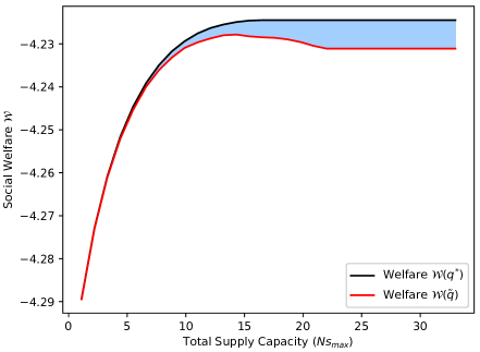
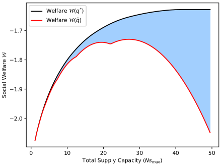
Figure 1: Welfare loss with increasing supply capacity and fixed inelastic demand. (Top) Nash equilibrium exists and the welfare loss does not grow unbounded. (Bottom) Nash equilibrium may not exist and the welfare loss grows unbounded.

Second, we examine the welfare loss between the two resulting welfares when the prosumers’ inelastic demands $d_{min}$ are varied while having their supply capacities $s_{max}$ fixed. On the top of Fig. 2, $s_{max}=0.7$ and $\beta_{i}=\left\{1.9+0.1i\;\middle|\;i=1,...,N\right\}$ are fixed while $d_{min}$ is decreased gradually from 5 to 0.7. The values of the latter two are selected using an ad-hoc technique so that the condition (21) for the existence and uniqueness of Nash equilibrium is satisfied for all prosumers. The figure shows that when the total inelastic demand is decreased, the welfare loss does not grow unbounded if a Nash equilibrium exists. Similarly, Fig. 2 on the bottom shows the welfare gap when $s_{max}=3$ and $\beta_{i}=\left\{0.5+0.1i\;\middle|\;i=1,...,N\right\}$ are fixed while $d_{min}$ is decreased from 5 to 0.7. The values of the latter two are selected such that, in this case, the resulting optimal allocations of the prosumers do not all necessarily satisfy (21) when their inelastic demands are below a certain threshold. Thus, a Nash equilibrium may not exist. The figure shows that the welfare loss grows unbounded when the total inelastic demand is decreased. In these simulations, the optimal allocations of prosumers 1 and 2 do not satisfy (21) when the total inelastic demand drops approximately below 20 and 11.5, respectively.

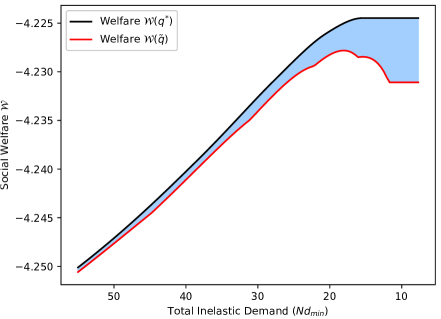
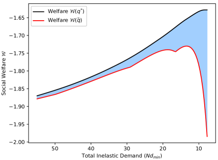
Figure 2: Welfare loss with decreasing inelastic demand and fixed supply capacity. (Top) Nash equilibrium exists and the welfare loss does not grow unbounded. (Bottom) Nash equilibrium may not exist and the welfare loss grows unbounded.

VI Conclusion and Future Directions

In this paper, a scalar-parameterized bidding mechanism has been proposed for the prosumers in a uniform-price peer-to-peer market. A competitive equilibrium and the associated efficient allocation have been established. When certain conditions on the action spaces of the prosumers are satisfied, we have shown that a unique Nash equilibrium exists. In addition, we have provided an efficient way to compute the market allocation at the Nash equilibrium, and in turn, the Nash equilibrium itself. Finally, a case study was given where we have shown that the welfare gap between the welfare at the competitive equilibrium and the welfare at the Nash equilibrium is bounded when the market supply or inelastic demand are varied. On the contrary when the existence of Nash equilibrium is not guaranteed, the welfare loss grows unbounded as the market supply is increased or the market inelastic demand is decreased. A future research direction would be to characterize a bound for the welfare loss. Also given that the proposed mechanism does not allow the prosumers to choose their preferred quantity of supply and demand separately, a future research direction would be to develop a mechanism which captures the dual nature of the prosumers.

Appendix A Proof of Theorem 1

We want to show that the first fundamental theorem of welfare economics holds for the proposed mechanism. This can be achieved by a standard approach in which the equilibrium conditions of (11) together with $\mu>0$ given by (9) is shown to be equivalent to the optimality conditions of the program (7) with a one-to-one correspondence. We first derive the optimality conditions for the prosumer’s problem, and then derive the optimality conditions for the market operator’s problem. Given that $q_{i}$ is given by (6) and since the prosumer is constrained by a maximum supply capacity $s_{max}$ (i.e. $-s_{max}\leq q_{i}$) along with the demand/supply balance constraint $\sum_{i=1}^{N}q_{i}=0$, then the action variable $\theta_{i}$ belongs to a compact, convex subset of $\mathbb{R}$. Given a price $\mu>0$, the second derivative of the prosumer’s payoff (11) with respect to the action variable $\theta_{i}$ is given by:

$$\frac{\partial^{2}\pi_{i}^{p}}{\partial\theta_{i}^{2}}=\frac{\partial^{2}S_{i}(Q(\theta_{i},\mu))}{\partial q_{i}^{2}}\Big{(}\frac{1}{\mu}\Big{)}^{2}$$ (22)

Since Assumption 1 implies that the second derivative of $S_{i}$ is non-positive, then (22) is non-positive. Hence, the prosumer’s payoff (11) is concave in $\theta_{i}$. Also, (11) is continuous by Assumption 1. As a result and since the Slater’s constraint qualification (strict feasibility) holds (i.e. there exists a $\theta_{i}$ such that $\theta_{i}{>}\mu(-s_{max}-d_{min})$), then the Karush-Kuhn-Tucker (KKT) conditions are necessary and sufficient for optimality for (11). Associate the Lagrange multiplier $\lambda$ with the inequality constraint for $\theta_{i}$ obtained from $-s_{max}\leq q_{i}$ and given by $\theta_{i}{\geq}\mu(-s_{max}-d_{min})$. Thus, the Lagrangian function becomes:

$$L(\theta_{i},\lambda)=S_{i}(q_{i})-q_{i}\mu+\lambda(\theta_{i}-\mu(-s_{max}-d_{min}))\vspace{-4pt}$$ (23)

Let $\theta_{i}^{*}$ denote an optimal action. Analyzing the KKT conditions shows that $\theta_{i}^{*}$ must satisfy:

$$\frac{\partial S_{i}(Q(\theta_{i}^{*},\mu))}{\partial q_{i}}=\mu,\ \text{if}\ \theta_{i}^{*}>\mu(-s_{max}-d_{min})$$ (24a)

$$\frac{\partial S_{i}(Q(\theta_{i}^{*},\mu))}{\partial q_{i}}<\mu,\ \text{if}\ \theta_{i}^{*}=\mu(-s_{max}-d_{min})\vspace{-6pt}$$ (24b)

Next, we analyze the convex optimization problem (7) that is solved by the market operator. The constraint (7c) along with the demand/supply balance constraint (7b) make the feasible solution set compact and convex. Therefore, the objective function is strictly concave and continuous in $q_{i}$, by Assumption 1, over a compact convex set. And since the Slater’s constraint qualification holds (i.e. there exists a $q_{i}$ such that $-s_{max}{<}q_{i},\forall i\in\mathcal{N}$), then the KKT conditions are necessary and sufficient for the solution of (7) to be optimal and unique. Associate the Lagrange multipliers $\eta$ with the equality constraint (7b) and $\lambda_{i},i\in\mathcal{N}$ with the inequality constraints (7c). Thus, the Lagrangian function becomes:

$$L(\bm{q},\eta,\bm{\lambda})=\sum_{i=1}^{N}S_{i}(q_{i})-\eta\Big{(}\sum_{i=1}^{N}q_{i}\Big{)}+\sum_{i=1}^{N}\lambda_{i}(q_{i}+s_{max})$$ (25)

Analyzing the KKT conditions gives the conditions for the unique optimal solution $\bm{q}^{*}$ and $\eta^{*}\geq 0$. The vector $\bm{q}^{*}$ must satisfy:

$$\frac{\partial S_{i}(q_{i}^{*})}{\partial q_{i}}=\eta^{*},\ \text{if}\ q_{i}^{*}>-s_{max}\vspace{-5pt}$$ (26a)

$$\frac{\partial S_{i}(q_{i}^{*})}{\partial q_{i}}<\eta^{*},\ \text{if}\ q_{i}^{*}=-s_{max}$$ (26b)

Also, the demand/supply balance constraint (7b) must hold for $q_{i}^{*}$:

$$\sum_{i=1}^{N}q_{i}^{*}=0\vspace{-0.1cm}$$ (27)

It is easy to show that if we let, by (6), $\theta_{i}=\eta^{*}(q_{i}^{*}-d_{min})$, then $(\bm{q}^{*},\eta^{*})$ satisfying (26) is equivalent to $(\bm{\theta},\eta^{*})$ satisfying (24). Also, (27) implies that $\eta^{*}=\mu$. Therefore, $(\bm{\theta},\mu)$ constitute a competitive equilibrium. Similarly it is easy to verify that if we let, by (6), $q_{i}=Q(\theta_{i}^{*},\mu)=d_{min}+\frac{\theta_{i}^{*}}{\mu}$, then $(\bm{\theta}^{*},\mu)$ satisfying (24) and (9) is equivalent to $\bm{q}$ satisfying (26). Therefore, $\bm{q}$ is an efficient allocation. Finally, uniqueness of the competitive equilibrium $(\bm{\theta}^{*},\mu)$ follows from its one-to-one correspondence with the unique optimal allocation $\bm{q}^{*}$.

Appendix B Proof of Lemma 1

The first derivative of the prosumer payoff (13) with respect to the action variable $\theta_{i}$ is given by:

$$\frac{\partial\pi_{i}^{p}(\theta_{i},\theta_{-i})}{\partial\theta_{i}}=\frac{\partial S_{i}(Q(\theta_{i},p(\bm{\theta})))}{\partial q_{i}}\frac{\partial Q(\theta_{i},p(\bm{\theta}))}{\partial\theta_{i}}{+}\frac{1}{N}{-}1$$ (28)

where:

$$\frac{\partial Q(\theta_{i},p(\bm{\theta}))}{\partial\theta_{i}}=\frac{-(\sum_{j\neq i}^{N}\theta_{j})Nd_{min}}{(\sum_{j=1}^{N}\theta_{j})^{2}}\vspace{-5pt}$$ (29)

Recall the assumption $\sum_{j=1}^{N}\theta_{j}{\leq}0$ from (9). Let $\sum_{j=1}^{N}\theta_{j}{<}0$. If $\sum_{j\neq i}^{N}\theta_{j}>0$, then (29) becomes strictly negative. Hence, (28) is strictly negative when Assumption 1 is satisfied. In other words, as $\theta_{i}$ is decreased (i.e. supply is increased), the payoff (13) increases without bound. Therefore, a Nash equilibrium cannot exist in this case. To investigate the two cases: $\bm{\theta}=\bm{0}$ and/or $\sum_{j\neq i}^{N}\theta_{j}=0$ and $\theta_{i}\neq 0$, we rewrite the payoff (13):

$$\begin{split}\pi_{i}^{p}(\theta_{i},\theta_{-i})=S_{i}(d_{min}(1-\frac{\theta_{i}}{\sum_{j=1}^{N}\theta_{j}}N))+\\ \frac{\sum_{j=1}^{N}\theta_{j}}{N}(1-\frac{\theta_{i}}{\sum_{j=1}^{N}\theta_{j}}N)\vspace{-5pt}\end{split}$$ (30)

Both terms in (30) can be positive or negative depending on the sign of $\theta_{i}$. If $\theta_{i}=0$, then the first term is zero and the second term is either zero or negative depending on whether $\sum_{j=1}^{N}\theta_{j}$ is zero or negative, respectively. Therefore, a Nash equilibrium cannot exist in the first case (i.e. $\bm{\theta}=\bm{0}$) since the payoff (30) can be increased from zero to a positive value by deviating from $\theta_{i}=0$. As a result, $\sum_{j=1}^{N}\theta_{j}{=}0$ is not possible. In the second case (i.e. $\sum_{j\neq i}^{N}\theta_{j}=0$ and $\theta_{i}\neq 0$), the payoff (30) can be increased from a negative value to zero by deviating from $\theta_{i}>0$ or $\theta_{i}<0$ to $\theta_{i}=0$. Therefore, a Nash equilibrium cannot exist in the second case.

Appendix C Proof of Lemma 2

If we let $N=2$ in (28) and follow the same argument in Lemma 1’s proof, it is easy to see that (28) can be negative or positive. Hence, the payoff (13) does not increase without bound as $\theta_{i}$ is decreased. Therefore, a Nash equilibrium may exist if $N=2$. Next, we want to show that the objective function for the prosumer is continuous and concave over a compact, convex set. Let $Q(\theta_{i},p(\bm{\theta}))=q_{i}$, i.e., replace $p$ in (6) by $p(\bm{\theta})$ from (9). To show that the prosumer’s payoff function (13) is concave in $\theta_{i}$, we examine the condition under which the second derivative of (13) is non-positive. The second derivative of (13) with respect to the action variable $\theta_{i}$ is given by:

$$\begin{split}\frac{\partial^{2}\pi_{i}^{p}}{\partial\theta_{i}^{2}}=\frac{\partial^{2}S_{i}(Q(\theta_{i},p(\bm{\theta})))}{\partial q_{i}^{2}}\Big{(}\frac{\partial Q(\theta_{i},p(\bm{\theta}))}{\partial\theta_{i}}\Big{)}^{2}+\\ \frac{\partial S_{i}(Q(\theta_{i},p(\bm{\theta})))}{\partial q_{i}}\Big{(}\frac{-2}{\sum_{j=1}^{N}\theta_{j}}\frac{\partial Q(\theta_{i},p(\bm{\theta}))}{\partial\theta_{i}}\Big{)}\end{split}$$ (31)

By Assumption 1, the first term in (31) is non-positive. And by Assumptions 1 and $\sum_{j=1}^{N}\theta_{j}{<}0$, the second term in (31) is non-negative. Making (31) less than or equal to zero yields the following condition:

$$\theta_{i}\geq-(\sum_{j\neq i}^{N}\theta_{j})\Big{(}\frac{Nd_{min}}{2}\frac{\frac{\partial^{2}S_{i}(Q(\theta_{i},p(\bm{\theta})))}{\partial q_{i}^{2}}}{\frac{\partial S_{i}(Q(\theta_{i},p(\bm{\theta})))}{\partial q_{i}}}+1\Big{)}\vspace{-5pt}$$ (32)

Define the set $\mathcal{A}$ by all possible $\theta_{i}$ in which (32) is satisfied. If $\theta_{i}\in\mathcal{A}$, then (31) is non-positive and hence the payoff function (13) is concave in $\theta_{i}$. Furthermore, (13) is continuous in $\theta_{i}$ where $\theta_{i}<-\sum_{j\neq i}^{N}\theta_{j}$ (the region derived in Lemma 1 in which Nash equilibrium may exist). When $\theta_{i}=-\sum_{j\neq i}^{N}\theta_{j}$, the price (9) is zero and (13) is undefined. Therefore, the prosumer’s payoff (13) is continuous and concave over a compact, convex subset of $\mathbb{R}$ which is defined by the intersection of (32) and $\theta_{i}\leq-\sum_{j\neq i}^{N}\theta_{j}-\epsilon$ where $\epsilon$ is any infinitesimal positive constant. To conclude, the above conditions constitute sufficient conditions for the existence of Nash equilibrium for the game $\mathcal{G}$.

Appendix D Proof of Theorem 2

To establish the uniqueness of market allocation $\bm{\tilde{q}}$ at a Nash equilibrium $\bm{\tilde{\theta}}$, we show that the players’ equilibrium conditions of (13) with $p(\bm{\theta})>0$ are equivalent to the optimality conditions of (16) with a one-to-one correspondence. The proof begins with deriving the sufficient conditions for existence of a Nash equilibrium. Then, we establish the existence and uniqueness of the market allocation at a Nash equilibrium. Next, we derive the necessary and sufficient KKT optimality conditions of (16). Finally, we show the one-to-one correspondence of the optimality conditions of (16) to the equilibrium conditions of (13) which concludes the uniqueness of a Nash equilibrium, completing the proof.

Sufficient Conditions for Nash Equilibria:

We showed, in Lemma 2’ proof, the conditions under which (13) is concave and continuous over a compact, convex set which result in a sufficient condition for the existence of Nash equilibria. Since the Slater’s constraint qualification holds (i.e. there exists a $\theta_{i}$ such that $\theta_{i}{>}p(\bm{\theta})(-s_{max}-d_{min})$), then the KKT optimality conditions of (13) are necessary and sufficient. Hereafter, we derive these conditions. Associate the Lagrange multiplier $\lambda$ with the inequality constraint for $\theta_{i}$ obtained from $-s_{max}{\leq}q_{i}$ and given by $\theta_{i}{\geq}p(\bm{\theta})(-s_{max}-d_{min})$. Given $p(\bm{\theta})$ as defined in (9), the Lagrangian function becomes:

$$L(\theta_{i},\lambda)=S_{i}(q_{i})-q_{i}p(\bm{\theta})+\lambda(\theta_{i}-p(\bm{\theta})(-s_{max}-d_{min}))$$ (33)

Let $\tilde{\theta_{i}}$ denote a Nash equilibrium. We let, by (6), $\tilde{\theta_{i}}=p(\bm{\tilde{\theta}})(Q(\tilde{\theta_{i}},p(\bm{\tilde{\theta}}))-d_{min})$ and invoke $\theta_{i}<-\sum_{j\neq i}^{N}\theta_{j}$ to analyze the KKT conditions. This shows that $\tilde{\theta_{i}}$ must satisfy:

$$\begin{split}\frac{\partial S_{i}(Q(\tilde{\theta_{i}},p(\bm{\tilde{\theta}})))}{\partial q_{i}}\Big{(}1+\frac{Q(\tilde{\theta_{i}},p(\bm{\tilde{\theta}}))}{(N-1)d_{min}}\Big{)}=p(\bm{\tilde{\theta}}),\\ \text{if}\ \tilde{\theta_{i}}>p(\bm{\tilde{\theta}})(-s_{max}-d_{min}))\end{split}$$ (34a)

$$\begin{split}\frac{\partial S_{i}(Q(\tilde{\theta_{i}},p(\bm{\tilde{\theta}})))}{\partial q_{i}}\Big{(}1+\frac{Q(\tilde{\theta_{i}},p(\bm{\tilde{\theta}}))}{(N-1)d_{min}}\Big{)}<p(\bm{\tilde{\theta}}),\\ \text{if}\ \tilde{\theta_{i}}=p(\bm{\tilde{\theta}})(-s_{max}-d_{min}))\end{split}$$ (34b)

Existence and Uniqueness of the Market Allocation:

We want to show that the objective function (16a) is continuous and strictly concave over a compact, convex set which implies the existence and uniqueness of the market allocation (i.e. optimal solution to (16)). Let $Q(\theta_{i},p(\bm{\theta}))=q_{i}$ (i.e. replace $p$ in (6) by $p(\bm{\theta})$ from (9)). The feasible set is a compact, convex subset of $\mathbb{R}$ since the prosumer is constrained by a maximum supply capacity $s_{max}$ (i.e. $-s_{max}\leq q_{i}$) and the demand/supply balance constraint $\sum_{i=1}^{N}q_{i}=0$. Next, the second derivative of $\tilde{S_{i}}(q_{i})$ with respect to $q_{i}$ (hence the objective function (16a)) is given by:

$$\begin{split}\frac{\partial^{2}\tilde{S_{i}}(q_{i})}{\partial q_{i}^{2}}=\frac{\partial^{2}S_{i}(q_{i})}{\partial q_{i}^{2}}\Big{(}1+\frac{q_{i}}{(N-1)d_{min}}\Big{)}+\\ \frac{\partial S_{i}(q_{i})}{\partial q_{i}}\frac{1}{(N-1)d_{min}}\end{split}\vspace{-10pt}$$ (35)

by Assumption 1, the objective function (16a) is concave in $q_{i}$ when:

$$q_{i}\geq-\Bigg{(}(N-1)d_{min}+\frac{\frac{\partial S_{i}(q_{i})}{\partial q_{i}}}{\frac{\partial^{2}S_{i}(q_{i})}{\partial q_{i}^{2}}}\Bigg{)}\vspace{-5pt}$$ (36)

Substitute $Q(\theta_{i},p(\bm{\theta}))=q_{i}$ in (36) to find the equivalent inequality for $\theta_{i}$. Let the set $\mathcal{B}$ be defined by all possible $\theta_{i}$’s in which the equivalent inequality for $\theta_{i}$ is satisfied. Then, $\mathcal{B}\subset\mathcal{A}$ where $\mathcal{A}$ is the set defined in Lemma 2’s proof under which the concavity of the prosumer’s objective function is guaranteed. However, it is worth noting that $\mathcal{A}\subset\mathcal{C}$ where $\mathcal{C}$ is the set defined by all possible $\theta_{i}$’s in which (16a) is concave in $\theta_{i}$.

Beside the region of concavity of (16a) in $q_{i}$, defined above in (36), we want to show that $\tilde{S_{i}}(q_{i}),i\in\mathcal{N}$ (hence (16a)) is strictly concave in $q_{i}$. To show this, let $q_{i},q_{i}^{\prime}\in\mathbb{R}$ where $-s_{max}\leq q_{i}<q_{i}^{\prime}$. Then, $\tilde{S_{i}}(q_{i})$ is strictly concave in $q_{i}$ when $\frac{\partial\tilde{S_{i}}(q_{i}^{\prime})}{\partial q_{i}^{\prime}}<\frac{\partial\tilde{S_{i}}(q_{i})}{\partial q_{i}}$. The first derivative of $\tilde{S_{i}}(q_{i})$ is given by:

$$\frac{\partial\tilde{S_{i}}(q_{i})}{\partial q_{i}}=(1+\frac{q_{i}}{(N-1)d_{min}})\frac{\partial S_{i}(q_{i})}{\partial q_{i}}$$ (37)

From (37) and by Assumption 1, it is easy to see that $\frac{\partial\tilde{S_{i}}(q_{i}^{\prime})}{\partial q_{i}^{\prime}}<\frac{\partial\tilde{S_{i}}(q_{i})}{\partial q_{i}}$. Hence, (16a) is strictly concave. Under the above conditions and the fact that $\tilde{S_{i}}(q_{i})$ is continuous in $q_{i}$, there exists a unique market allocation profile $\bm{\tilde{q}}$.

Necessary and Sufficient Conditions for the Market Allocation:

Given that the Slater’s constraint qualification holds for (16), then the KTT optimality conditions are necessary and sufficient. Associate the Lagrange multipliers $\eta$ with the equality constraint and $\lambda_{i},i\in\mathcal{N}$ with the inequality constraints. The Lagrangian function becomes:

$$L(\bm{q},\eta,\bm{\mu})=\sum_{i=1}^{N}\tilde{S_{i}}(q_{i})-\eta\Big{(}\sum_{i=1}^{N}q_{i}\Big{)}+\sum_{i=1}^{N}\lambda_{i}(q_{i}+s_{max})$$ (38)

Let $\tilde{\bm{q}}$ be the unique optimal solution to (16). Analyzing the KKT conditions shows that $\tilde{\bm{q}}$ and $\tilde{\eta}$ must satisfy:

$$\frac{\partial S_{i}(\tilde{q_{i}})}{\partial\tilde{q_{i}}}(1+\frac{\tilde{q_{i}}}{(N-1)d_{min}})=\tilde{\eta},\ \text{if}\ \tilde{q_{i}}>-s_{max}$$ (39a)

$$\frac{\partial S_{i}(\tilde{q_{i}})}{\partial\tilde{q_{i}}}(1+\frac{\tilde{q_{i}}}{(N-1)d_{min}})<\tilde{\eta},\ \text{if}\ \tilde{q_{i}}=-s_{max}$$ (39b)

Uniqueness of the Nash Equilibrium:

Analogous to the analysis in the last paragraph of Theorem 1’s proof, it is straightforward to conclude the one-to-one correspondence of (34) and (39). Therefore, uniqueness of the Nash equilibrium follows from the corresponding unique market allocation. That is, uniqueness of the Nash equilibrium follows from the one-to-one correspondence of $(\bm{\tilde{q}},\tilde{\eta})$ to $\bm{\tilde{\theta}}$ with $\tilde{\eta}=p(\bm{\tilde{\theta}})$.

References

- [1] F. P. Kelly, A. K. Maulloo, and D. K. H. Tan, “Rate control for communication networks: shadow prices, proportional fairness and stability,” Journal of the Operational Research society, vol. 49, pp. 237–252, 1998.
- [2] R. Johari and J. N. Tsitsiklis, “Efficiency loss in a network resource allocation game,” Mathematics of Operations Research, vol. 29, no. 3, pp. 407–435, 2004.
- [3] W. Vickrey, “Counterspeculation, auctions, and competitive sealed tenders,” The Journal of finance, vol. 16, no. 1, pp. 8–37, 1961.
- [4] E. H. Clarke, “Multipart pricing of public goods,” Public choice, pp. 17–33, 1971.
- [5] T. Groves, “Incentives in teams,” Econometrica: Journal of the Econometric Society, pp. 617–631, 1973.
- [6] R. T. Maheswaran and T. Başar, “Nash equilibrium and decentralized negotiation in auctioning divisible resources,” Group Decision and Negotiation, vol. 12, no. 5, pp. 361–395, 2003.
- [7] R. Maheswaran and T. Başar, “Efficient signal proportional allocation (espa) mechanisms: Decentralized social welfare maximization for divisible resources,” IEEE Journal on Selected Areas in Communications, vol. 24, no. 5, pp. 1000–1009, 2006.
- [8] R. Johari and J. N. Tsitsiklis, “Parameterized supply function bidding: Equilibrium and efficiency,” Operations research, vol. 59, no. 5, pp. 1079–1089, 2011.
- [9] P. D. Klemperer and M. A. Meyer, “Supply function equilibria in oligopoly under uncertainty,” Econometrica: Journal of the Econometric Society, pp. 1243–1277, 1989.
- [10] W. Lin and E. Bitar, “A structural characterization of market power in electric power networks,” IEEE Transactions on Network Science and Engineering, vol. 7, no. 3, pp. 987–1006, 2019.
- [11] M. Ndrio, K. Alshehri, and S. Bose, “A scalar-parameterized mechanism for two-sided markets,” IFAC-PapersOnLine, vol. 53, no. 2, pp. 16 952–16 957, 2020.
- [12] Y. Parag and B. K. Sovacool, “Electricity market design for the prosumer era,” Nature energy, vol. 1, no. 4, pp. 1–6, 2016.
- [13] W. Saad, Z. Han, H. V. Poor, and T. Başar, “Game-theoretic methods for the smart grid: An overview of microgrid systems, demand-side management, and smart grid communications,” IEEE Signal Processing Magazine, vol. 29, no. 5, pp. 86–105, 2012.
- [14] Y. Xu, N. Li, and S. H. Low, “Demand response with capacity constrained supply function bidding,” IEEE Transactions on Power Systems, vol. 31, no. 2, pp. 1377–1394, 2015.
- [15] T. Başar and G. J. Olsder, Dynamic Noncooperative Game Theory. SIAM, 1998.
- [16] K. Alshehri, M. Ndrio, S. Bose, and T. Başar, “Quantifying market efficiency impacts of aggregated distributed energy resources,” IEEE Transactions on Power Systems, vol. 35, no. 5, pp. 4067–4077, 2020.
- [17] B. Gharesifard, T. Başar, and A. D. Domínguez-García, “Price-based coordinated aggregation of networked distributed energy resources,” IEEE Transactions on Automatic Control, vol. 61, no. 10, pp. 2936–2946, 2015.
- [18] E. Tsybina, J. Burkett, and S. Grijalva, “The effect of prosumer duality on power market: evidence from the cournot model,” IEEE Transactions on Power Systems, vol. 38, no. 1, pp. 692–701, 2022.