Deep Learning in Deterministic Computational Mechanics

 

Abstract

The rapid growth of deep learning research, including within the field of computational mechanics, has resulted in an extensive and diverse body of literature. To help researchers identify key concepts and promising methodologies within this field, we provide an overview of deep learning in deterministic computational mechanics. Five main categories are identified and explored: simulation substitution, simulation enhancement, discretizations as neural networks, generative approaches, and deep reinforcement learning. This review focuses on deep learning methods rather than applications for computational mechanics, thereby enabling researchers to explore this field more effectively. As such, the review is not necessarily aimed at researchers with extensive knowledge of deep learning — instead, the primary audience is researchers at the verge of entering this field or those who attempt to gain an overview of deep learning in computational mechanics. The discussed concepts are, therefore, explained as simple as possible.

Keywords: Deep learning; Computational mechanics, Neural networks; Surrogate model; Physics-informed; Generative

Contents

1. 1 Introduction
   1. 1.1 Motivation
   2. 1.2 Taxonomy of Deep Learning Techniques in Computational Mechanics
   3. 1.3 Deep Learning
2. 2 Simulation Substitution
   1. 2.1 Data-Driven Modeling
      1. 2.1.1 Space-Time Approaches
         1. 2.1.1.1 Fully-Connected Neural Networks
         2. 2.1.1.2 Image-To-Image Mapping
         3. 2.1.1.3 Model Order Reduction Encoding
         4. 2.1.1.4 Neural Operators
         5. 2.1.1.5 Neural Network Approximation Power
         6. 2.1.1.6 Active Learning & Transfer Learning
      2. 2.1.2 Time-Stepping Procedures
         1. 2.1.2.1 Recurrent Neural Networks
         2. 2.1.2.2 Dynamic Mode Decomposition
   2. 2.2 Physics-Informed Learning
      1. 2.2.1 Space-Time Approaches
         1. 2.2.1.1 Differential Equation Solving With Neural Networks
         2. 2.2.1.2 Inverse Problems
      2. 2.2.2 Time-Stepping Procedures
         1. 2.2.2.1 Physics-Informed Neural Networks
         2. 2.2.2.2 Inverse Problems
      3. 2.2.3 Enforcement Of Physics By Construction
3. 3 Simulation Enhancement
   1. 3.1 Pre-processing
      1. 3.1.1 Data Preparation
      2. 3.1.2 Initialization
      3. 3.1.3 Meshing
   2. 3.2 Physical Modeling
      1. 3.2.1 Model Substitution
      2. 3.2.2 Identification Of Model Parameters
      3. 3.2.3 Model Identification
   3. 3.3 Numerical Methods
      1. 3.3.1 Algorithm Enhancement
      2. 3.3.2 Multiscale Methods
      3. 3.3.3 Optimization
   4. 3.4 Post-Processing
4. 4 Discretizations As Neural Networks
   1. 4.1 Finite Element Method
   2. 4.2 Finite Difference Method
   3. 4.3 Material Discretizations
   4. 4.4 Neural Differential Equations
5. 5 Generative Approaches
   1. 5.1 Autoencoders
   2. 5.2 Generative Adversarial Networks
   3. 5.3 Diffusion Models
   4. 5.4 Applications
      1. 5.4.1 Data Generation
      2. 5.4.2 Generative Design & Design Optimization
      3. 5.4.3 Conditional Generation
      4. 5.4.4 Anomaly Detection
6. 6 Deep Reinforcement Learning
   1. 6.1 Applications
      1. 6.1.1 Extensions
7. 7 Conclusion
8. A Deep Reinforcement Learning
   1. A.1 Deep Policy Networks
   2. A.2 Deep Q-Learning

1 Introduction

1.1 Motivation

In recent years, access to enormous quantities of data combined with rapid advances in machine learning has yielded outstanding results in computer vision, recommendation systems, medical diagnosis, and financial forecasting [1]. Nonetheless, the impact of learning algorithms reaches far beyond and has already found its way into many scientific disciplines [2].

The rapid interest in machine learning in general and within computational mechanics is well documented in the scientific literature. By considering the number of publications treating “Artificial Intelligence”, “Machine Learning”, “Deep Learning”, and “Neural Networks”, the interest can be quantified. Figure 1(a) shows the trend in all journals of Elsevier and Springer since 1999, while Figure 1(b) depicts the trend within the computational mechanics community by considering representative journals at Elsevier and Springer. The trends before 2017 differ slightly, with a steady growth in general but only limited interest within computational mechanics. However, around 2017, both curves show a shift in trend, namely a vast increase in publications highlighting the interest and potential prospects of artificial intelligence and its subtopics for a variety of applications.

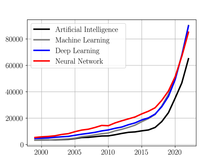
(a) Publications in all fields.

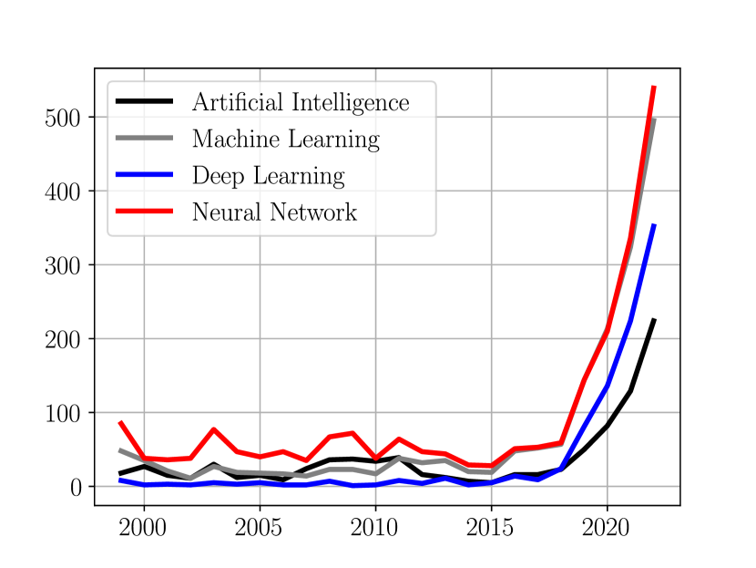
(b) Publications within Computational Mechanics.

Figure 1: Number of publications concerning artificial intelligence and some of its subtopics since 1999. Illustration inspired by [3].

1.2 Taxonomy of Deep Learning Techniques in Computational Mechanics

Due to the rapid growth [4] in deep learning research, as also seen in Figure 1(a), we provide an overview of the various deep learning methodologies in deterministic computational mechanics. Numerous review articles on deep learning for specific applications have already emerged (see [5, 6] for topology optimization, [7] for full waveform inversion, [8, 9, 10, 11, 12] for fluid mechanics, [13] for continuum mechanics, [14] for material mechanics, [15] for constitutive modeling, [16] for generative design, [17] for material design, and [18] for aeronautics). The aim of this work is, however, to focus on the general methods rather than applications, where similar methods are often applied to different problems. This has the potential to bridge gaps between scientific communities by highlighting similarities between methods and thereby establishing clarity on the state-of-the-art. We propose the following taxonomy in order to discuss the deep learning methods in a structured manner:

• simulation substitution (Section 2)

  • data-driven modeling (Section 2.1)

  • physics-informed learning (Section 2.2)

• simulation enhancement (Section 3)

• discretizations as neural networks (Section 4)

• generative approaches (Section 5)

• deep reinforcement learning (Section 6)

Simulation substitution replaces the entire simulation with a surrogate model, which in this work are neural networks (NNs). The model can be trained with supervised learning, which purely relies on labeled data and therefore is referred to as data-driven modeling. The generalization errors of these models can be reduced by physics-informed learning. Here, physics constraints are imposed on the learnable space such that only physically admissible solutions are learned.

Simulation enhancement instead only replaces components of the simulation chain, while the remaining parts are still handled by classical methods. Approaches within this category are strongly linked to their respective applications and will, therefore, be presented in the context of their specific use cases. Both data-driven and physics-informed approaches will be discussed.

Treating discretizations as neural networks is achieved by constructing a discretization from the basic building blocks of NNs, i.e., linear transformations and non-linear activation functions. Thereby, techniques within deep learning frameworks – such as automatic differentiation, gradient-based optimization, and efficient GPU-based parallelization – can be leveraged to improve classical simulation techniques.

Generative approaches deal with creating new content based on a data set. The goal is not, however, to recreate the data, but to generate statistically similar data. This is useful in diversifying the design space or enhancing a data set to train surrogate models.

Finally, in deep reinforcement learning, an agent learns how to interact with an environment in order to maximize rewards provided by the environment. In the case of deep reinforcement learning, the agent is modeled with NNs. In the context of computational mechanics, the environment is modeled by the governing physical equations. Reinforcement learning provides an alternative to gradient-based optimization, which is useful when gradient information is not available.

1.3 Deep Learning

Before continuing with the topics specific to computational mechanics, NNs and the notation used throughout this work are briefly introduced. In essence, NNs are function approximators that are capable of approximating any continuous function [26]. The NN parametrized by the parameters $\boldsymbol{\theta}$ learns a function $\hat{y}=f_{NN}(x;\boldsymbol{\theta})$, which approximates the relation $y=f(x)$. The NN is constructed with nested linear transformations in combination with non-linear activation functions $\sigma$. The quality of prediction is determined by a cost function $C(\hat{y})$, which is to be minimized. Its gradients $\nabla_{\boldsymbol{\theta}}C$ with respect to the parameters $\boldsymbol{\theta}$ are used within a gradient-based optimization [23, 27, 28] to update the parameters $\boldsymbol{\theta}$ and thereby improve the prediction $\hat{y}$. Supervised learning relies on labeled data $x^{\mathcal{M}},y^{\mathcal{M}}$ to establish a cost function, while unsupervised learning does not rely on labeled data. The parameters defining the user-defined training algorithm and NN architecture are referred to as hyperparameters.

Notational Remark 1

Although $x$ and $y$ may denote vector-valued quantities, we do not use bold-faced notation for them. Instead, this is reserved for all $N$ degrees of freedom within a problem, i.e., $\boldsymbol{x}=\{x_{i}\}_{i=1}^{N}$, $\boldsymbol{y}=\{y_{i}\}_{i=1}^{N}$. This can, for instance, be in the form of a domain $\Omega$ sampled with $N$ grid points or systems composed of $N$ degrees of freedom. Note however, that matrices will still be denoted with capital letters in bold face.

Notational Remark 2

A multitude of NN architectures will be discussed throughout this work, for which we introduce abbreviations and subscripts. Most prominent are fully-connected NNs $F_{FNN}$ (FC-NNs) [29, 23], convolutional NNs $f_{CNN}$ (CNNs) [30, 31, 32], recurrent NNs $f_{RNN}$ (RNNs) [33, 34, 35], and graph NNs $f_{GNN}$ (GNNs) [36, 37, 38]. If the network architecture is independent of the method, the network is denoted as $f_{NN}$.

2 Simulation Substitution

In the field of computational mechanics, numerical procedures are developed to solve or find partial differential equations (PDEs). A generic PDE can be written as

$$\mathcal{N}[u;\lambda]=0,\qquad\text{on }\Omega\times\mathcal{T},$$ (1)

where a non-linear operator $\mathcal{N}$ acts on a solution $u(x,t)$ of a PDE as well as the coefficients $\lambda(x,t)$ of the PDE in the spatio-temporal domain $\Omega\times\mathcal{T}$. In the forward problem, the solution $u(x,t)$ is to be computed, while the inverse problem considers either the non-linear operator $\mathcal{N}$ or coefficients $\lambda(x,t)$ as unknowns.

A further distinction is made between methods treating the temporal dimension $t$ as a continuum, as in space-time approaches [42] (Sections 2.1.1 and 2.2.1), or in discrete sequential time steps, as in time-stepping procedures (Sections 2.1.2 and 2.2.2). For simplicity, but without loss of generality, time-stepping procedures will be presented on PDEs with a first order derivative with respect to time:

$$\frac{\partial u}{\partial t}=\mathcal{N}[u;\lambda],\qquad\text{on }\Omega\times\mathcal{T}.$$ (2)

Another task in computational mechanics is the forward modeling and identification of systems of ordinary differential equations (ODEs). For this, we will consider systems of the following form:

$$\frac{d\boldsymbol{x}(t)}{dt}=\boldsymbol{f}(\boldsymbol{x}(t)).$$ (3)

Here, $\boldsymbol{x}(t)$ are the time-dependent degrees of freedom and $\boldsymbol{f}$ is the right-hand side defining the system of equations. Both the forward problem of computing $\boldsymbol{x}(t)$ and the inverse problem of identifying $\boldsymbol{f}$ will be discussed in the following.

2.1 Data-Driven Modeling

Data-driven modeling relies entirely on labeled data $x^{\mathcal{M}},y^{\mathcal{M}}$. The NN learns the mapping between $x^{\mathcal{M}}$ and $y^{\mathcal{M}}$ with $\hat{y}_{i}=f_{NN}(x_{i};\boldsymbol{\theta})$. Thereby an interpolation to yet unseen datapoints is established. A data-driven loss $\mathcal{L}_{\mathcal{D}}$, such as the mean squared error, for example, can be used as cost function $C$.

$$C=\mathcal{L}_{\mathcal{D}}=\frac{1}{2N_{\mathcal{D}}}\sum_{i=1}^{N_{\mathcal{D}}}||\hat{y}_{i}-y_{i}^{\mathcal{M}}||^{2}_{2}$$ (4)

2.1.1 Space-Time Approaches

To declutter the notation, but without loss of generality, the temporal dimension $t$ is dropped in this section, as it is possible to treat it like any other spatial dimension $x$ in the scope of these methods. The goal of the upcoming methods is to either learn a forward operator $\hat{u}=F[\lambda;x]$, an inverse operator for the coefficients $\hat{\lambda}=I[u;x]$, or an inverse operator for the non-linear operator $\hat{\mathcal{N}}=O[u;\lambda;x]$. The methods will be explained using the forward operator, but they apply analogously to the inverse operators. Only the inputs and outputs differ.

The solution prediction $\hat{u}_{i}$ at coordinate $x_{i}$ or $\boldsymbol{\hat{u}}_{i}$ on the entire domain $\Omega$ is made based on a set of inverse coefficients $\boldsymbol{\lambda}_{i}$. The cost function $C$ is formulated analogously to Equation 4:

$$C=\mathcal{L}_{\mathcal{D}}=\frac{1}{2N_{\mathcal{D}}}\sum_{i=1}^{N_{\mathcal{D}}}||\hat{u}_{i}-u_{i}^{\mathcal{M}}||_{2}^{2}\qquad\textrm{or}\qquad C=\mathcal{L}_{\mathcal{D}}=\frac{1}{2N_{\mathcal{D}}}\sum_{i=1}^{N_{\mathcal{D}}}||\boldsymbol{\hat{u}}_{i}-\boldsymbol{u}_{i}^{\mathcal{M}}||_{2}^{2}.$$ (5)

2.1.1.1 Fully-Connected Neural Networks

The simplest procedure is to approximate the operator $F$ with a FC-NN $F_{FNN}$.

$$\hat{u}(x)=F_{FNN}(\boldsymbol{\lambda};x;\boldsymbol{\theta})$$ (6)

Example applications are flow classification [43, 44], fluid flow in turbomachinery [45], dynamic beam displacements from previous measurements [46], wall velocity predictions in turbulence [47], heat transfer [48], prediction of source terms in turbulence models [49], full waveform inversion [50, 51, 52], and topology optimization based on moving morphable bars [53]. The approach is however limited to simple problems, as an abundance of data is required. Therefore, several improvements have been proposed.

2.1.1.2 Image-To-Image Mapping

One downside of the application of fully-connected NNs to problems in computational mechanics is that they often need to learn spatial relationships with respect to $x$ from scratch. CNNs inherently account for these spatial relationships due to their kernel-based structure. Therefore, image-to-image mappings using CNNs have been proposed, where an image, i.e., a uniform grid (see Figure 2) of the coefficients $\boldsymbol{\lambda}$, is used as input.

$$\boldsymbol{\hat{u}}=F_{CNN}(\boldsymbol{\lambda};\boldsymbol{\theta})$$ (7)

This results in a prediction of the solution $\boldsymbol{\hat{u}}$ throughout the entire image, i.e., the domain.

Figure 2: Representation of nodes of a Cartesian grid as pixels in an image. Adapted from [54].

Applications include pressure and velocity predictions around airfoils [55, 56, 57, 58], stress predictions from geometries and boundary conditions [59, 60], steady flow predictions [61], detection of manufacturing features [62, 63], full waveform inversion [64, 65, 66, 67, 68, 69, 70, 71, 72, 73, 74, 75], and topology optimization [76, 77, 78, 79, 80, 81, 82, 83, 84, 85]. An important choice in the design of the learning algorithm is the encoding of the input data. In the case of geometries and boundary conditions, binary representations are the most straightforward approach. These are however challenging for CNNs, as discussed in [61]. Signed distance functions [61] or simulations on coarse grids provide superior alternatives. For inverse problems, an initial forward simulation of an initial guess of the inverse field can be used to encode the desired boundary conditions [80, 83, 84, 85]. Another possibility for CNNs is a decomposition of the domain. The mapping can be performed on the full domain [86], smaller subdomains [87], or even individual pixels [88]. In the latter two cases, interfaces require special treatment.

2.1.1.3 Model Order Reduction Encoding

The disadvantage of CNN mappings is being constrained to uniform grids on rectangular domains. This can be circumvented by using GNNs, such as in [89, 90, 91], or point cloud-based NNs [92, 93], such as in [94]. To further aid the learning, the NN can be applied to a lower-dimensional space that is able to capture the data. For complex problems, mappings $e$ to low-dimensional spaces (also referred to as latent space or latent vector) $\boldsymbol{h}$ can be identified with model order reduction techniques. Thus, in the case of simulation substitution, a low-dimensional encoding $\boldsymbol{h}^{\lambda}=e(\boldsymbol{\lambda})$ of $\boldsymbol{\lambda}$ is identified. This is provided as input to a NN to predict the solution field $\boldsymbol{h}^{u}$ in a reduced latent space. The full solution field $\boldsymbol{u}$ is obtained in a decoding $d=e^{-1}$ step. The prediction is given as

$$\boldsymbol{\hat{u}}=d(\boldsymbol{\hat{h}}^{u})=d\bigl{(}F_{NN}(\boldsymbol{h}^{\lambda};\boldsymbol{\theta})\bigr{)}=d\Bigl{(}F_{NN}\bigl{(}e(\boldsymbol{\lambda});\boldsymbol{\theta}\bigr{)}\Bigr{)}.$$ (8)

The dimensional reduction can, e.g., be performed with principal components analysis [95, 96], as proposed in [97], proper orthogonal decomposition [98], or reduced manifold learning [99]. These techniques have been applied to learning aortic wall stresses [100], arterial wall stresses [101], flow velocities in viscoplastic flow [102], and the inverse problem of identifying unpressurized geometries from pressurized geometries [103]. Currently, the most impressive results in data-driven surrogate modeling are achieved with model order reduction encodings combined with NNs [104, 105], which can be combined with most other methodologies presented in this work.

Another dimensionality reduction technique are autoencoders [106], where $e$ and $d$ are modeled by NNs. These are treated in detail in Section 5.1 and enable non-linear encodings. An early investigation is presented in [107], where proper orthogonal decomposition is related to NNs. Application areas are the prediction of designs of acoustic scatterers from the reduced latent space [108], or mappings from dynamic responses of bridges to damage [109]. Furthermore, it has to be stated that many of the image-to-image mapping techniques rely on NN architectures inspired by autoencoders, such as U-nets [110, 111].

2.1.1.4 Neural Operators

The most recent trend in surrogate modeling with NNs are neural operators [112], which map between function spaces instead of functions. Neural operators rely on the extension of the universal approximation theorem [26] to non-linear operators [113]. The two most prominent neural operators are DeepONets [114] and Fourier neural operators [115].

DeepONet

In DeepONets [114], illustrated in Figure 3, the task of predicting the operator $\hat{u}(\boldsymbol{\lambda};x)$ is split up into two sub-tasks:

• the prediction of $N_{P}$ basis functions $\boldsymbol{\hat{t}}(x)$ (TrunkNet),

• the prediction of the corresponding $N_{P}$ problem-specific coefficients $\boldsymbol{\hat{b}}(\boldsymbol{\lambda})$ (BranchNet).

The basis is predicted by the TrunkNet with parameters $\boldsymbol{\theta}^{T}$ via an evaluation at coordinates $x$. The coefficients are estimated from the coefficients $\boldsymbol{\lambda}$ using the BranchNet parametrized by $\boldsymbol{\theta}^{B}$ and, thus, specific to the problem being solved. Taking the dot product over the evaluated basis and the coefficients yields the solution prediction $\hat{u}(\boldsymbol{\lambda};x)$.

$$\boldsymbol{\hat{t}}(x) =F^{T}_{FNN}(x;\boldsymbol{\theta}^{T})$$ (9)

$$\boldsymbol{\hat{b}}(\boldsymbol{\lambda}) =F^{B}_{FNN}(\boldsymbol{\lambda};\boldsymbol{\theta}^{B})$$ (10)

$$\hat{u}(x) =\boldsymbol{\hat{b}}(\boldsymbol{\lambda})\cdot\boldsymbol{\hat{t}}(x)$$ (11)

Figure 3: DeepONet, operator learning via prediction of the basis functions $\boldsymbol{\hat{t}}$ and the corresponding coefficients $\boldsymbol{\hat{b}}$ [114].

Applications can be found in [116, 117, 118, 119, 120, 121, 122, 123, 124, 125, 126, 127, 128]. DeepONets have also been extended with physics-informed loss functions [129, 130, 131].

Fourier Neural Operators

Fourier neural operators [115] predict the solution $\boldsymbol{\hat{u}}$ on a uniform grid $\boldsymbol{x}$ from the spatially varying coefficients $\boldsymbol{\lambda}=\lambda(\boldsymbol{x})$. As the aim is to learn a mapping between functions, sampled on the entire domain, non-local mappings can be performed at each layer [132]. For example, mappings such as integral kernels [133, 134], Laplace transformations [135], and Fourier transforms [115] can be employed. These transformations enhance the non-local expressivity of the NN [132], where Fourier transforms are particularly favorable due to the computational efficiency achievable through fast Fourier transforms.

The Fourier neural operator, as illustrated in Figure 4, consists of Fourier layers, where linear transformations $\boldsymbol{K}$ are performed after Fourier transforms $\mathcal{F}$ along the spatial dimensions $x$. Subsequently, an inverse Fourier transform $\mathcal{F}^{-1}$ is applied, which is added to the output of a linear transformation $\boldsymbol{W}$ performed outside the Fourier space. Thus, the Fourier transform can be skipped by the NN. The final step is an activation function $\sigma$. The manipulations within a Fourier layer to predict the next activation on the uniform grid $\boldsymbol{a}^{(j+1)}(\boldsymbol{x})$ can be written as

$$\boldsymbol{a}^{(j+1)}(\boldsymbol{x})=\sigma\bigg{(}\boldsymbol{W}\boldsymbol{a}^{(j)}(\boldsymbol{x})+\boldsymbol{b}+(\mathcal{F}^{-1}\Bigl{[}\boldsymbol{K}\mathcal{F}\bigl{[}\boldsymbol{a}^{(j)}(\boldsymbol{x})\bigr{]}\Bigr{]}\bigg{)},$$ (12)

where $\boldsymbol{b}$ is the bias. Both the linear transformations $\boldsymbol{K},\boldsymbol{W}$ and the bias $\boldsymbol{b}$ are learnable and thereby part of the parameters $\boldsymbol{\theta}$. Multiple Fourier layers can be employed, typically used in combination with an encoding network $P_{NN}$ and a decoding network $Q_{NN}$.

Figure 4: Fourier neural operator, operator learning in the Fourier space [115].

Applications can be found in [136, 137, 138, 139, 140, 141, 142, 143, 144, 145, 146]. An extension relying on the attention mechanisms of transformers [147] is presented in [148]. Analogously to DeepONets, Fourier neural operators have been combined with physics-informed loss functions [149].

2.1.1.5 Neural Network Approximation Power

Despite the advancements in NN architectures, NN surrogates struggle to learn solutions of general PDEs. Typically, successes have only been achieved for parametrized PDEs with relatively small parameter spaces – or in cases where accuracy, reliability, or generalization were disregarded. It has, however, been shown – both for simple architectures such as FC-NNs [150, 151] as well as for advanced architectures such as DeepONets [152] – that NNs possess an excellent theoretical approximation power which can capture solutions of various PDEs. Currently, there are two obstacles that impede the identification of sufficiently good optima with these desirable NN parameter spaces [150]:

• training data: generalization error,

• training algorithm: optimization error.

A lack of sufficient training data leads to poor generalization. This might be alleviated through faster data generation using, e.g., faster and specialized classical methods [153], or improved sampling strategies, i.e., finding the minimum number of required datapoints distributed in a specific manner to train the surrogate. Additionally, current training algorithms only converge to local optima. Research into improved optimization algorithms, such as current trends in computing better initial weights [154] and thereby better local optima, attempts to reduce the optimization error. At the same time, training times are reduced drastically increasing the competitiveness.

2.1.1.6 Active Learning & Transfer Learning

Finally, an important machine learning technique independent of the NN architecture is active learning [155]. Instead of precomputing a labeled data set, data is only provided when the prediction quality of the NN is insufficient. Furthermore, the data is not chosen arbitrarily, but only in the vicinity of the failed prediction. In computational mechanics, the prediction of the NN can be assessed with an error indicator. For an insufficient result, the results of a classical simulation are used to retrain the NN. Over time, the NN estimates improve in the respective domain of application. Due to the error indicator and the classical simulations, the predictions are reliable. Examples for active learning in computational mechanics can be found in [156, 157, 158].

Another technique, transfer learning [159, 160], aims at accelerating the NN training. Here, the NN is first trained on a similar task. Subsequently, it is applied to the task of interest – where it converges faster than an untrained NN. Applications in computational mechanics can be found in [73, 161].

2.1.2 Time-Stepping Procedures

For the time-stepping procedures, we will consider Equations 2 and 3 in the following.

2.1.2.1 Recurrent Neural Networks

The simplest approach to modeling time series data is by using FC-NNs to predict the next time step $t_{i+1}$ from the current time step $t_{i}$:

$$\hat{u}(x,t_{i+1})=F_{FNN}\bigl{(}x,t_{i};u(x,t_{i});\boldsymbol{\theta}\bigr{)}.$$ (13)

However, this approach lacks the ability to capture the temporal dependencies between different time steps, as each input is treated independently and without considering more than just the previous time step. Incorporating the sequential nature of the data can be achieved directly with RNNs. RNNs maintain a hidden state which captures information from the previous time steps, to be used for the next time step prediction. By unrolling the RNN, the entire time-history can be predicted.

$$\{\hat{u}(x,t_{2}),\hat{u}(x,t_{3}),\dots,\hat{u}(x,t_{N})\}=F_{RNN}(x;u(x,t_{1});\boldsymbol{\theta})$$ (14)

Shortcomings of RNNs, such as their tendency to struggle with learning long-term dependencies due to the problem of vanishing or exploding gradients, have been addressed by more sophisticated architectures such as long short-time memory networks (LSTM) [34], gated recurrent unit networks (GRU) [162], and transformers [147]. The concept of recurrent units has also been combined with other architectures, as demonstrated for CNNs [163] and GNNs [164, 165, 166, 167, 89, 90, 168].

Further applications of RNNs are full waveform inversion [169, 170, 171], high-dimensional chaotic systems [172], fluid flow [173, 3], fracture propagation [91], sensor signals in non-linear dynamic systems [174, 175], and settlement field predictions induced by tunneling [176], which was extended to damage prediction in affected structures [177, 178]. RNNs are often combined with reduced order model encodings [179], where the dynamics are predicted on the reduced latent space, as demonstrated in [180, 181, 182, 183, 184, 185, 186]. Further variations employ classical time-stepping schemes on the reduced latent space obtained by autoencoders [187, 188].

2.1.2.2 Dynamic Mode Decomposition

Another approach that was formulated for system dynamics, i.e., Equation 3 is dynamic mode decomposition (DMD) [189, 190]. The aim of DMD is to identify a linear operator $\boldsymbol{A}$ that relates two successive snapshot matrices with $n$ time steps $\boldsymbol{X}=[\boldsymbol{x}(t_{1}),\boldsymbol{x}(t_{2}),\dots,\boldsymbol{x}(t_{n})]^{T},\boldsymbol{X}^{\prime}=[\boldsymbol{x}(t_{2}),\boldsymbol{x}(t_{3}),\dots,\boldsymbol{x}(t_{n+1})]^{T}$:

$$\boldsymbol{X}^{\prime}\approx\boldsymbol{A}\boldsymbol{X}.$$ (15)

To solve this, the problem is reframed as a regression task. The operator $\boldsymbol{A}$ is approximated by minimizing the Frobenius norm of the difference between $\boldsymbol{X}^{\prime}$ and $\boldsymbol{A}\boldsymbol{X}$. This minimization can be performed using the Moore-Penrose pseudoinverse $\boldsymbol{X}^{\dagger}$ (see, e.g., [191]):

$$\boldsymbol{A}=\underset{{\boldsymbol{A}}}{\text{arg min}}||\boldsymbol{X}^{\prime}-\boldsymbol{A}\boldsymbol{X}||_{F}=\boldsymbol{X}^{\prime}\boldsymbol{X}^{\dagger}.$$ (16)

Once the operator is identified, it can be used to propagate the dynamics forward in time, approximating the next state $\boldsymbol{x}(t_{i+1})$ using the current state $\boldsymbol{x}(t_{i})$:

$$\boldsymbol{x}(t_{i+1})\approx\boldsymbol{A}\boldsymbol{x}(t_{i}).$$ (17)

This framework, is however, only valid for linear dynamics. DMD can be extended to handle non-linear systems through the application of Koopman operator theory [192]. According to Koopman operator theory, it is possible to represent a non-linear system as a linear one by using an infinite-dimensional Koopman operator $\mathcal{K}$ that acts on a transformed state $e(\boldsymbol{x}(t_{i}))$:

$$g(\boldsymbol{x}(t_{i+1}))=\mathcal{K}[e(\boldsymbol{x}(t_{i}))].$$ (18)

In theory, the Koopman operator $\mathcal{K}$ is an infinite-dimensional linear transformation. In practice, however, finite-dimensional approximations are employed. This approach is, for example utilized in the extended DMD [193], where the regression from Equation 16 is performed on a higher-dimensional state $\boldsymbol{h}(t_{i})=e(\boldsymbol{x}(t_{i}))$ relying on a dictionary of orthonormal basis functions $\boldsymbol{\psi}(\boldsymbol{x})$. Alternatively, the dictionary can be learned using NNs, i.e., $\boldsymbol{\hat{\psi}}(\boldsymbol{x})=\psi_{NN}(\boldsymbol{x};\boldsymbol{\theta})$, as demonstrated in [194, 195]. The NN is trained by minimizing the mismatch between predicted state $\boldsymbol{\psi}(\boldsymbol{\hat{x}}(t_{i+1}))=\boldsymbol{A}\boldsymbol{\hat{\psi}}(\boldsymbol{x}(t_{i}))$ (Equation 17) and the true state in the dictionary space. Orthogonality is not required and therefore not enforced.

$$C=\frac{1}{2N}\sum_{i=1}^{N}||\boldsymbol{\hat{\psi}}(\boldsymbol{x}(t_{i+1}))-\boldsymbol{A}\boldsymbol{\hat{\psi}}(\boldsymbol{x}(t_{i}))||_{2}^{2}$$ (19)

When the dictionary is learned, the state predictions can be reconstructed using the Koopman mode decomposition, as explained in detail in [194].

Alternatively, the mapping to the augmented state can be performed with autoencoders, which at the same time allows for a direct map back to the original space [196, 197, 198, 199]. Thus, an encoder learns a reduced latent space $\boldsymbol{\hat{h}}(\boldsymbol{x})=e_{NN}(\boldsymbol{x};\boldsymbol{\theta}^{e})$ and a decoder learns the inverse mapping $\boldsymbol{\hat{x}}(\boldsymbol{h})=d_{NN}(\boldsymbol{h};\boldsymbol{\theta}^{d})$. The networks are trained using three losses: the autoencoder reconstruction loss $\mathcal{L}_{\mathcal{A}}$, the linear dynamics loss $\mathcal{L}_{\mathcal{R}}$, and the future state prediction loss $\mathcal{L}_{\mathcal{F}}$.

$$\mathcal{L}_{\mathcal{A}} =\frac{1}{2(n+1)}\sum_{i=1}^{n+1}||\boldsymbol{x}(t_{i})-d_{NN}(e_{NN}(\boldsymbol{x}(t_{i});\boldsymbol{\theta}^{e});\boldsymbol{\theta}^{d})||_{2}^{2}$$ (20)

$$\mathcal{L}_{\mathcal{R}} =\frac{1}{2n}\sum_{i=1}^{n}||e_{NN}(\boldsymbol{x}(t_{i+1});\boldsymbol{\theta}^{e})-\boldsymbol{A}e_{NN}(\boldsymbol{x}(t_{i});\boldsymbol{\theta}^{e})||_{2}^{2}$$ (21)

$$\mathcal{L}_{\mathcal{F}} =\frac{1}{2n}\sum_{i=1}^{n}||\boldsymbol{x}(t_{i+1})-d_{NN}(\boldsymbol{A}e_{NN}(\boldsymbol{x}(t_{i});\boldsymbol{\theta}^{e});\boldsymbol{\theta}^{d})||_{2}^{2}$$ (22)

$$C =\kappa_{\mathcal{A}}\mathcal{L}_{\mathcal{A}}+\kappa_{\mathcal{R}}\mathcal{L}_{\mathcal{R}}+\kappa_{\mathcal{F}}\mathcal{L}_{\mathcal{F}}$$ (23)

The cost function $C$ is composed of a weighted sum of the loss terms $\mathcal{L}_{\mathcal{A}},\mathcal{L}_{\mathcal{R}},\mathcal{L}_{\mathcal{F}}$ and weighting terms $\kappa_{\mathcal{A}},\kappa_{\mathcal{R}},\kappa_{\mathcal{F}}$. Furthermore, [198] allows $\boldsymbol{A}$ to vary depending on the state. This is achieved by predicting the eigenvalues of $\boldsymbol{A}$ with an auxiliary network and constructing the matrix from these.

2.2 Physics-Informed Learning

In supervised learning, as discussed in Section 2.1, the quality of prediction strongly depends on the amount of training data. Acquiring data in computational mechanics may be expensive. To reduce the amount of required data, constraints enforcing the physics have been proposed. Two main approaches exist. The physics can be enforced by modifying the cost function through a penalty term punishing unphysical predictions, thus acting as a regularizer. Possible modifications are discussed in the upcoming section. Alternatively, the physics can be enforced by construction, i.e., by reducing the learnable space to a physically meaningful space. This approach is highly specific to its application and will therefore mainly be explored in Section 3. A brief coverage is provided in Section 2.2.3.

2.2.1 Space-Time Approaches

Once again and without loss of generality, the temporal dimension $t$ is dropped to declutter the notation. However, in contrast to Section 2.1.1, the following methods are not equally applicable to forward and inverse problems. Thus, the prediction of the solution $\hat{u}$, the PDE coefficients $\hat{\lambda}$, and the non-linear operator $\mathcal{N}$ are treated separately.

2.2.1.1 Differential Equation Solving With Neural Networks

The concept of solving PDEs was first proposed in the 1990s [200, 201, 202], but was recently popularized by the so-called physics-informed neural networks (PINNs) [203] (see [204, 205, 206] for recent review articles and SciANN [207], SimNet [208], DeepXDE [209] for libraries).

To illustrate the idea and variations of PINNs, we will consider the differential equation of a static elastic bar

$$\frac{d}{dx}\left(EA\frac{du}{dx}\right)+p=0,\qquad x\in\Omega.$$ (24)

Here, the non-linear operator $\mathcal{N}$ is given by the left-hand side of the equation, the solution $u(x)$ is the axial displacement, and the spatially varying coefficients $\lambda(x)$ are given by the cross-sectional properties $EA(x)$ and the distributed load $p(x)$. Additionally, boundary conditions are specified, which can be in terms of Dirichlet (on $\Gamma_{D}$) or Neumann boundary conditions (on $\Gamma_{N}$):

$$u(x) =g(x),\qquad x\in\Gamma_{D},$$ (25)

$$EA(x)\frac{du(x)}{dx} =f(x),\qquad x\in\Gamma_{N}.$$ (26)

Physics-Informed Neural Networks

PINNs [203] approximate either the solution $u(x)$, the coefficients $\lambda(x)$, or both with FC-NNs.

$$\hat{u}(x) =F_{FNN}(x;\boldsymbol{\theta}^{u})$$ (27)

$$\hat{\lambda}(x) =I_{FNN}(x;\boldsymbol{\theta}^{\lambda})$$ (28)

Instead of training the network with labeled data as in Equation 5, the residual of the PDE is considered. The residual is evaluated at a set of $N_{\mathcal{N}}$ points, called collocation points. Taking the mean squared error over the residual evaluations yields the PDE loss

$$\mathcal{L}_{\mathcal{N}}=\frac{1}{2N_{\mathcal{N}}}\sum_{i}^{N_{\mathcal{N}}}||\mathcal{N}[u(x_{i});\lambda(x_{i})]||^{2}_{2}=\frac{1}{2N_{\mathcal{N}}}\sum_{i}^{N_{\mathcal{N}}}\left(\frac{d}{dx}\left(EA(x_{i})\frac{du(x_{i})}{dx}\right)+p(x_{i})\right)^{2}.$$ (29)

The gradients of the possible predictions, i.e., $u,EA$, and $p$ with respect to $x$, are obtained with automatic differentiation [210] through the NN approximation. Similarly, the boundary conditions are enforced at the $N_{\mathcal{B_{D}}}+N_{\mathcal{B_{N}}}$ boundary points.

$$\mathcal{L}_{\mathcal{B}}=\frac{1}{2N_{\mathcal{N}_{D}}}\sum_{i}^{N_{\mathcal{B}_{D}}}(u(x_{i})-g)^{2}+\frac{1}{2N_{\mathcal{B}_{N}}}\sum_{i}^{N_{\mathcal{B}_{N}}}\left(EA(x_{i})\frac{du(x_{i})}{dx}-f\right)^{2}$$ (30)

The cost function is composed of the PDE loss $\mathcal{L}_{\mathcal{N}}$, boundary loss $\mathcal{L}_{\mathcal{B}}$, and possibly a data-driven loss $\mathcal{L}_{\mathcal{D}}$

$$C=\mathcal{L}_{\mathcal{N}}+\mathcal{L}_{\mathcal{B}}+\mathcal{L}_{\mathcal{D}}.$$ (31)

Both the deep least-squares method [211] and the deep Galerkin method [212] are closely related. Instead of focusing on the residuals at individual collocation points as in PINNs, these methods consider the $L^{2}$-norm of the residuals integrated over the domain $\Omega$.

Variational Physics-Informed Neural Networks

Computing high-order derivatives for the non-linear operator $\mathcal{N}$ is expensive. Therefore, variational PINNs [213, 214] consider the weak form of the PDE, which lowers the order of differentiation. In the case of the bar equation, the weak PDE loss is given by

$$\mathcal{L}_{\mathcal{V}}=\int_{\Omega}\frac{dw(x)}{dx}EA(x)\frac{du(x)}{dx}d\Omega-\int_{\Gamma_{N}}w(x)EA(x)\frac{du(x)}{dx}d\Gamma_{N}-\int_{\Omega}w(x)p(x)d\Omega=0,\forall w(x).$$ (32)

In [213], trigonometric and polynomial test functions $w(x)$ are used. The cost function is obtained by replacing the PDE loss $\mathcal{L}_{\mathcal{N}}$ with the weak PDE loss $\mathcal{L}_{\mathcal{V}}$ in Equation 31. Note that the Neumann boundary conditions are now not included in the boundary loss $\mathcal{L}_{\mathcal{B}}$, as they are already incorporated in the weak form in Equation 32. The integrals are evaluated through numerical integration methods, such as Gaussian quadrature, Monte Carlo integration methods [215, 216], or sparse grid quadratures [217]. Severe inaccuracies can be introduced through the numerical integration of the NN output – for which remedies have been proposed in [218].

Weak Adversarial Networks

Instead of specifying the test functions $w(x)$, weak adversarial networks [219] employ a second NN as test function

$$\hat{w}(x)=W_{FNN}(x;\boldsymbol{\theta}^{w}).$$ (33)

The test function is learned through a minimax optimization

$$\min_{\boldsymbol{\theta}^{u}}\max_{\boldsymbol{\theta}^{w}}C,$$ (34)

where the test function $w(x)$ continually challenges the solution $u(x)$.

Deep Energy Method & Deep Ritz Method

By minimizing the potential energy $\Pi=\Pi_{i}+\Pi_{e}$ instead, the need for test functions is overcome by the deep energy method [220] and the deep Ritz method [221]. This results in the following loss term

$$\mathcal{L}_{\mathcal{E}}=\Pi_{i}+\Pi_{e}=\frac{1}{2}\int_{\Omega}EA(x)\left(\frac{du(x)}{dx}\right)^{2}d\Omega-\int_{\Gamma}u(x)EA(x)\frac{du(x)}{dx}d\Gamma-\int_{\Omega}u(x)p(x)d\Omega.$$ (35)

Note that the inverse problem generally cannot be solved using the minimization of the potential energy. Consider, for instance, the potential energy of the bar equation in Equation 35, which is not well-posed in the inverse setting. Here, $EA(x)$ going towards $-\infty$ in the domain $\Omega$ and going towards $\infty$ at $\Gamma_{N}$ minimizes the potential energy $\mathcal{L}_{\mathcal{E}}$.

Extensions

A multitude of extensions to the PINN methodology exist. For in-depth reviews, see [204, 205, 206].

Learning Multiple Solutions
Currently, PINNs are mainly employed to learn a single solution. As the training effort exceeds the solving effort of classical solvers, the viability of PINNs is questionable [222]. However, PINNs can also be employed to learn multiple solutions. This is achieved by providing the parametrization of the PDE, i.e., $\lambda$ as an additional input to the network, as discussed in Section 2. This enables a cheap prediction stage without retraining for new solutions. One possible example for this is [223], where different geometries are captured in terms of point clouds and processed with point cloud-based NNs [92].

Boundary Conditions
The enforcement of the boundary conditions through a penalty term $\mathcal{L}_{\mathcal{B}}$ in Equation 30 leads to an unbalanced optimization, due to the competing loss terms $\mathcal{L}_{\mathcal{N}},\mathcal{L}_{\mathcal{B}},\mathcal{L}_{\mathcal{D}}$ in Equation 31. One remedy is to modify the NN output $F_{FNN}$ by multiplication of a function, such that the Dirichlet boundary conditions are satisfied a priori, i.e., $\mathcal{L}_{\mathcal{B}}=0$, as demonstrated in [224, 20].

$$\hat{u}(x)=G(x)+D(x)F_{FNN}(x;\boldsymbol{\theta}^{u})$$ (36)

Here, $G(x)$ is a smooth interpolation of the boundary conditions, and $D(x)$ is a signed distance function that is zero at the boundary. For Neumann boundary conditions, [225] propose to predict $u$ and its derivatives $\partial u/\partial x$ with separate networks, such that the Neumann boundary conditions can be enforced strongly by modifying the derivative network. This requires an additional constraint, ensuring that the derivative predictions match the derivative of $u$. For complex domains, $G(x)$ and $D(x)$ cannot be found analytically. Therefore, [224] use NNs to learn $G(x)$ and $D(x)$ in a supervised manner by prescribing either the boundary values or zero at the boundary and restricting the values within the domain to be non-zero. Similarly [226] proposed using radial basis function networks for $G(x)$, where $D(x)=1$ is assumed. The radial basis function networks are determined by solving a linear system of equations constructed with the boundary conditions. On uniform grids, strong enforcement can be achieved through specialized CNN kernels [185] with constant padding terms for Dirichlet boundary conditions and ghost cells for Neumann boundary conditions. Constrained backward propagation [227] has also been proposed to guarantee the enforcement of boundary conditions [228, 229].

Another possibility is to introduce weighting terms $\kappa_{\mathcal{N}},\kappa_{\mathcal{B}},\kappa_{\mathcal{D}}$ for each loss term. These are either hyperparameters, or they are learned during the optimization with attention mechanisms [230, 231, 232]. This is achieved by performing a minimax optimization with respect to all weighting terms $\boldsymbol{\kappa}=\{\kappa_{\mathcal{N}},\kappa_{\mathcal{B}},\kappa_{\mathcal{D}}\}$

$$\min_{\boldsymbol{\theta}}\max_{\boldsymbol{\kappa}}C.$$ (37)

Expanding on this idea, each collocation point used for the loss terms can be considered an individual equality constraint [233, 234]. Therefore, a weighting term $\kappa_{\mathcal{N}_{i}}$ is allocated for each collocation point $x_{i}$, as illustrated for the PDE loss $\mathcal{L}_{\mathcal{N}}$ from Equation 29

$$\mathcal{L}_{\mathcal{N}}=\frac{1}{2N_{\mathcal{N}}}\sum_{i}^{N_{\mathcal{N}}}\kappa_{\mathcal{N},i}||\mathcal{N}[u(x_{i});\lambda(x_{i})]||^{2}_{2}.$$ (38)

This has the added advantage that greater emphasis is assigned on more important collocation points, i.e., points which lead to larger residuals. This approach is strongly related to the approaches relying on the augmented Lagrangian method [235] and competitive PINNs [236], where an additional NN models the penalty weights $\kappa(x)=K_{FNN}(x;\boldsymbol{\theta}^{\kappa})$. This is similar to weak adversarial networks, but instead formulated using the strong form.

Ansatz
Another prominent topic is the question of which ansatz to choose. The type of ansatz is, for example, determined by different NN architectures (see [237] for a comparison) or combinations with classical ansatz formulations. Instead of using FC-NNs, some authors [238, 163] employ CNNs to exploit the spatial structure of the data. Irregular geometries can be handled by embedding the structure in a rectangular domain using binary encodings [239] or signed distance functions [61, 240]. Another option are coordinate transformations into rectangular grids [241]. The CNN requires a full-grid discretization, meaning that the coordinates $x$ are analytically independent of the prediction $\hat{u}=F_{CNN}$. Thus, the gradients of $u$ are not obtained with automatic differentiation, but with numerical differentiation, i.e., finite differences. Alternatively, the output of the CNN can represent coefficients of an interpolation, as proposed under the name spline-PINNs [242] using Hermite splines. This again allows for an automatic differentiation. This is similarly applied for irregular geometries in [243], where GNNs are used in combination with a piecewise polynomial basis. Using a classical basis has the added advantage that Dirichlet boundary conditions can be satisfied exactly. A further variation is the approximation of the coefficients of classical bases with FC-NNs. This is shown with B-splines in [244] in the sense of isogeometric analysis [245]. This was similarly done for piecewise polynomials in [246]. However, instead of simply minimizing the PDE residual from Equation 29 directly, the finite element discretization [247, 248] is exploited. The loss $\mathcal{L}_{\mathcal{F}}$ can thus be formulated in terms of the non-linear stiffness matrix $\boldsymbol{K}$, the force vector $\boldsymbol{F}$, and the degrees of freedom $\boldsymbol{u}^{h}$.

$$\mathcal{L}_{\mathcal{F}}=||\boldsymbol{K}(\boldsymbol{u}^{h})\boldsymbol{u}^{h}-\boldsymbol{F}||_{2}^{2}$$ (39)

In the forward problem, $\boldsymbol{u}^{h}$ is approximated by a FC-NN, whereas for the inverse problem a FC-NN predicts $\boldsymbol{K}$. Similarly, [249, 250] map a NN onto a finite element space by using the NN evaluations at nodal coordinates as the corresponding basis function coefficents. This also allows a straightforward strong enforcement of Dirichlet boundary conditions, as demonstrated in [54] with CNNs. The nodes are represented as pixels (see Figure 2).

Prior information on the solution can be incorporated through a feature layer [251]. If, for example, it is known that the solution is composed of trigonometric functions, a feature layer with trigonometric functions can be applied after the input layer. Thus, known features are given to the NN directly to aid the learning. Without known features, the task can also be modified to improve learning. Inspired by adaptivity from finite elements, refinements are progressively learned by additional layers of the NN [252] (see Figure 5). Thus, a coarse solution $\boldsymbol{u}_{1}$ is learned to begin with, then refined to $\boldsymbol{u}_{2}$ by an additional layer, which again is refined to $\boldsymbol{u}_{3}$ until the deepest refinement level is reached.

Figure 5: Refinement expressed with NNs in terms of NN depth. Thick black lines indicate non-learnable connections and gray lines indicate learnable connections. Each added layer is composed of a projection from the coarser level and a correction obtained through the learnable connection.

Domain Decomposition
To improve the scalability of PINNs to more complex problems, several domain decomposition methods have been proposed. One approach are hp-variational PINNs [214], where the domain is decomposed into patches. Piecewise polynomial test functions are defined on each patch separately, while the solution is approximated by a globally acting NN. This enables a separate numerical integration of each patch, improving its accuracy.

In an alternative formulation, one NN can be used per subdomain. This was proposed as conservative PINNs [253], where conservation laws are enforced at the interface to ensure continuity. Here, the discrepancies between both solution and flux were penalized at the interface in a least squares manner. The advantages of this approach are twofold: Firstly, parallelization is possible [254] and, secondly, adaptivitiy can be introduced. Shallower networks can be employed for smooth solutions and deeper networks for more complex solutions. The approach was generalized for any PDE in the context of extended PINNs [255]. Here, the interface condition is formulated in terms of the difference in both the residual and the solution.

Acceleration Methods
Analogously to supervised learning, as discussed in Section 2.1, transfer learning can be applied to PINNs [256] as, e.g., demonstrated in phase-field fracture [257] or topology optimization [258]. These are very suitable problems since crack and displacement fields evolve with mostly local changes in phase-field fracture. For topology optimization, only minor updates are expected between each optimization iteration [258].

The poor performance of PINNs in their original form can also be improved with better sampling strategies. In importance sampling [259, 260], the collocation point density is proportional to the value of the cost function. Alternatively, residual-based adaptive refinement [209] adds collocation points in the vicinity of areas with a higher cost function.

Another essential topic for NNs is normalization of the inputs, outputs, and loss terms [261, 262]. For time-dependent problems, it is possible to use time-dependent normalization [263] to ensure that the solution is always in the same range regardless of the time step.

Furthermore, the cost function can be enhanced by including the derivative of the residual [264] as well. The derivative should also be minimized, as both the residual and its derivative should be zero at the correct solution. However, a general problem in the cost function formulation persists. The cost function should correspond to the norm of the error, which is not necessarily the case. This means that a reduction in the cost does not necessarily yield an improvement in quality of solution. The error norm can be expressed in terms of the $H^{-1}$-norm, which, according to [265], can efficiently be computed on rectangular domains with Fourier transforms. Thus, the $H^{-1}$-norm can directly be used as cost function and minimized.

Another aspect is numerical differentiation, which is advantageous for the residual of the PDE [266], as automatic differentiation may be erroneous due to spurious oscillations between collocation points. Thus, numerical differentiation enforces regularity, which was exploited in [266] by coupling automatic differentiation and numerical differentiation to retain the advantages of automatic differentiation.

Further specialized modifications to NN architectures have been proposed. Adaptive activation functions [267] have shown acceleration in convergence. Extreme learning machines [268, 269] remove the need for iterations altogether. All layers are randomly initialized in extreme learning machines, and only the last layer is learnable. Without a non-linear activation function, the parameters are found with a least-squares regression. This was demonstrated for PINNs in [270]. Instead of only learning the last layer, the problem can be split into a non-linear and a linear regression problem, which are solved separately [271], such that the full expressivity of NNs is retained.

Applications To Forward Problems

PINNs have been applied to various PDEs (see [204, 205, 206] for an overview). Forward problems can, for example, be found in solid mechanics [261, 272, 273], fluid mechanics [274, 275, 276, 277, 278, 279, 280, 281], and thermomechanics [282, 283]. Currently, PINNs do not outperform classical solvers such as the finite element method [284, 222] in terms of speed for a given accuracy of engineering relevance. In the author’s experience and judgement, this is especially the case for forward problems even if the extensions mentioned above are employed. Often, the mentioned gains compared to classical forward solvers disregard the training effort and only report evaluation times.

Incorporating large parts of the solution in the form of measurements with the data-driven loss $\mathcal{L}_{\mathcal{D}}$ improves the performance of PINNs, which thereby can become a viable method in some cases. Yet, [285] states that data-driven methods outperform PINNs. Thus PINNs should not be regarded as a replacement for data-driven methods, but rather as a regularization technique for data-driven methods to reduce the generalization error.

Applications To Inverse Problems

However, PINNs are in particular useful for inverse problems with full domain knowledge, i.e., the solution is available throughout the entire domain. This has, for example, been shown for the identification of material properties [286, 287, 288, 262, 289]. In contrast, for inverse problems with only partial knowledge, the applicability of PINNs is limited [290], as both forward and inverse solution have to be learned simultaneously. Most applications therefore limit themselves to simpler inversions such as size and shape optimization. Examples are published, e.g., in [291, 272, 292, 293, 294, 295, 296]. Exceptions that deal with the identification of entire fields can be found in full waveform inversion [297], topology optimization [298], elasticity, and the heat equation [299].

2.2.1.2 Inverse Problems

PINNs are capable of discovering governing equations by either learning the operator $\mathcal{N}$ or the coefficients $\lambda$. The resulting operator is, however, not always interpretable, and in the case of identification of the coefficients, the underlying PDE is assumed. To discover interpretable operators, one can apply sparse regression approaches [300]. Here, potential differential operators are assumed as an input to the non-linear operator

$$\hat{\mathcal{N}}\left[x,u,\frac{\partial u}{\partial x},\frac{\partial^{2}u}{\partial x^{2}},\dots\right]=0.$$ (40)

Subsequently, a NN learns the corresponding coefficients using observed solutions inserted into Equation 40. The evaluation of the differential operators is achieved through automatic differentiation by first interpolating the solution with a NN. Sparsity is ensured with a $L^{1}$-regularization.

A more sophisticated and complete framework is AI-Feynman [301]. Sequentially, dimensional analysis, polynomial regression, and brute force search algorithms are applied to identify fundamental laws in the data. If unsuccessful, a NN interpolates the data, which can thereby be queried for symmetry and separability. The identification of symmetries leads to a reduction in variables, i.e., a reduction of the input space. In the case of separability, the problem is decomposed into two subproblems. The reduced problems or subproblems are iteratively fed through the framework until an equation is identified. AI-Feynman has been successfully applied to 100 equations from the Feynman lectures [302].

2.2.2 Time-Stepping Procedures

Again Equation 2 and Equation 3 will be considered for the time-stepping procedures.

2.2.2.1 Physics-Informed Neural Networks

In the spirit of domain decomposition, parareal PINNs [303] split up the temporal domain in subdomains $[t_{i}<t_{i+1}]$. A rough estimate of the solution $u$ is provided by a conjugate gradient solver on a simplified form of the PDE starting from $t_{0}$. PINNs are then independently applied in each subdomain to correct the estimate. Subsequently, the conjugate gradient solver is applied again, starting from $t_{1}$. This process is repeated until all time steps have been traversed. A closely related approach can be found in [304], where a PINN is retrained on successive time segments. It is however ensured that previous time steps are kept fulfilled through a data-driven loss term for time segments that were already learned.

Another approach are the discrete-time PINNs [203], which consider the temporal dimension in a discrete manner. The differential equation from Equation 2 is discretized with the Runge-Kutta method with $q$ stages [305]:

$$u^{n+c_{i}} =u^{n}+\Delta t\sum_{j=1}^{q}a_{ij}\mathcal{N}[u^{n+c_{j}}],\qquad i=1,\dots,q,$$ (41)

$$u^{n+1} =u^{n}+\Delta t\sum_{j=1}^{q}b_{j}\mathcal{N}[u^{n+c_{j}}],$$ (42)

where

$$u^{n+c_{j}}(x)=u(t^{n}+c_{j}\Delta t,x),\qquad j=1,\dots,q.$$ (43)

A NN $F_{NN}$ predicts all stages $i=1,\dots,q$ from an input $x$:

$$\boldsymbol{\hat{u}}=[\hat{u}^{n+c_{1}}(x),\dots,\hat{u}^{n+c_{q}}(x),\hat{u}^{n+1}(x)]=F_{NN}(x;\boldsymbol{\theta}).$$ (44)

The cost is then constructed by rearranging Equations 41 and 42.

$$\hat{u}^{n} =\hat{u}_{i}^{n}=\hat{u}^{n+c_{i}}-\Delta t\sum_{j=1}^{q}a_{ij}\mathcal{N}[\hat{u}^{n+c_{j}}],\qquad i=1,\dots,q,$$ (45)

$$\hat{u}^{n} =\hat{u}^{n}_{q+1}=\hat{u}^{n+1}-\Delta t\sum_{j=1}^{q}b_{j}\mathcal{N}[\hat{u}^{n+c_{j}}].$$ (46)

The $q+1$ predictions $\hat{u}_{i}^{n},\hat{u}^{n}_{q+1}$ of $\hat{u}^{n}$ have to match the initial conditions $u^{\mathcal{M}^{n}}$, where the mean squared error is used as a loss function to learn all stages $\boldsymbol{\hat{u}}$. The approach has been applied to fluid mechanics [306, 307].

2.2.2.2 Inverse Problems

As for inverse problems in the space-time approaches (Paragraph 2.2.1.2), the non-linear operator $\mathcal{N}$ can be learned. For temporal problems, this corresponds to the right-hand side of Equation 2 for PDEs and to Equation 3 for systems of ODEs. The predicted right-hand side can then be used to predict time series using a classical time-stepping scheme, as proposed in [308]. More sophisticated methods leaning on similar principles are presented in the following. Specifically, we will discuss PDE-Net for discovering PDEs, SINDy for discovering systems of ODEs in an interpretable sense, and an approach relying on multistep methods for systems of ODEs. The multistep approach leads to a non-interpretable, but more expressive approximation of the right-hand side.

PDE-Net

PDE-Net [309, 310] is designed to learn both the system dynamics $u(x,t)$ and the underlying differential equation it follows. Given a problem of the form of Equation 2, the right-hand side can be approximated as a function of coordinates and gradients of the solution.

$$\hat{\mathcal{N}}\left[x,u,\frac{\partial u}{\partial x},\frac{\partial^{2}u}{\partial x^{2}},\dots\right]$$ (47)

The operator $\hat{\mathcal{N}}$ is approximated by NNs. The first step involves estimating spatial derivatives using learnable convolutional filters. The filters are designed to adjust their order of approximation based on the fit to the underlying measurements $u^{\mathcal{M}}$, while the type of gradient is predefined. Thus, the NN learns how to best approximate spatial derivatives specific to the underlying data. Subsequently, the inputs of $\hat{\mathcal{N}}$ are combined with point-wise CNNs [311] in [309] or a symbolic network in [310]. Both yield an interpretable operator from which the analytical expression can be extracted. In order to construct a loss function, Equations 2 and 47 are discretized using the forward Euler method:

$$u(x,t_{n+1})=u(x,t_{n})+\Delta t\hat{\mathcal{N}}\left[x,u,\frac{\partial u}{\partial x},\frac{\partial^{2}u}{\partial x^{2}},\dots\right].$$ (48)

This temporal discretization is applied iteratively, and the discrepancy between the derived function and the measured data $u^{\mathcal{M}}(x,t_{n})$ serves as the loss function.

SINDy

Sparse identification of non-linear dynamic systems (SINDy) [312] deals with the discovery of dynamic systems of the form of Equation 3. The task is posed as a sparse regression problem. Snapshot matrices of the state $\boldsymbol{X}=[\boldsymbol{x}(t_{1}),\boldsymbol{x}(t_{2}),\dots,\boldsymbol{x}(t_{n})]$ and its time derivative $\dot{\boldsymbol{X}}=[\dot{\boldsymbol{x}}(t_{1}),\dot{\boldsymbol{x}}(t_{2}),\dots,\dot{\boldsymbol{x}}(t_{n})]$ are related to one another via candidate functions $\boldsymbol{\Theta}(\boldsymbol{X})$ evaluated at $\boldsymbol{X}$ using unknown coefficients $\boldsymbol{\Xi}$:

$$\dot{\boldsymbol{X}}=\boldsymbol{\Theta}(\boldsymbol{X})\boldsymbol{\Xi}.$$ (49)

The coefficients $\boldsymbol{\Xi}$ are determined through sparse regression, such as sequential thresholded least squares or LASSO regression. By including partial derivatives, SINDy has been extended to the discovery of PDEs [313, 314].

The expressivity of SINDy can further be increased by a coordinate transformation into a representation allowing for a simpler representation of the system dynamics. This can be achieved with an autoencoder (consisting of an encoder $e_{NN}(x;\boldsymbol{\theta}^{e})$ and a decoder $d_{NN}(h;\boldsymbol{\theta}^{d})$, as proposed in [315], where the dynamics are learned on the reduced latent space $h$ using SINDy. A simultaneous optimization of the NN parameters $\boldsymbol{\theta}^{e},\boldsymbol{\theta}^{d}$ and SINDy parameters $\boldsymbol{\Xi}$ is conducted with gradient descent. The cost is defined in terms of the autoencoder reconstruction loss $\mathcal{L}_{\mathcal{A}}$ and the residual of Equation 49 at both the reduced latent space $\mathcal{L}_{\mathcal{R}}$ and the original space $\mathcal{L}_{\mathcal{F}}$. A $L^{1}$-regularization for $\boldsymbol{\Xi}$ promotes sparsity.

$$\mathcal{L}_{\mathcal{A}} =\frac{1}{2n}\sum_{i=1}^{n}||\boldsymbol{x}(t_{i})-d_{NN}\big{(}e_{NN}(\boldsymbol{x}(t_{i});\boldsymbol{\theta}^{e});\boldsymbol{\theta}^{d}\big{)}||_{2}^{2}$$ (50)

$$\mathcal{L}_{\mathcal{R}} =\frac{1}{2n}\sum_{i=1}^{n}||\underbrace{\Big{(}\nabla_{x}e_{NN}\big{(}\boldsymbol{x}(t_{i});\boldsymbol{\theta}^{e}\big{)}\Big{)}\cdot\dot{\boldsymbol{x}}(t_{i})}_{\dot{\boldsymbol{h}}}-\boldsymbol{\Theta}\Big{(}e_{NN}\big{(}\boldsymbol{x}(t_{i});\boldsymbol{\theta}^{e}\big{)}\Big{)}\boldsymbol{\Xi}||_{2}^{2}$$ (51)

$$\mathcal{L}_{\mathcal{F}} =\frac{1}{2n}\sum_{i=1}^{n}||\dot{\boldsymbol{x}}(t_{i})-\nabla_{h}d_{NN}\big{(}\underbrace{e_{NN}(\boldsymbol{x}(t_{i});\boldsymbol{\theta}^{e})}_{\boldsymbol{h}};\boldsymbol{\theta}^{d}\big{)}\cdot\underbrace{\boldsymbol{\Theta}\Big{(}e_{NN}(\boldsymbol{x}(t_{i});\boldsymbol{\theta}^{e})\Big{)}\boldsymbol{\Xi}}_{\dot{\boldsymbol{h}}}||_{2}^{2}$$ (52)

$$C =\kappa_{\mathcal{A}}\mathcal{L}_{\mathcal{A}}+\kappa_{\mathcal{R}}\mathcal{L}_{\mathcal{R}}+\kappa_{\mathcal{F}}\mathcal{L}_{\mathcal{F}}$$ (53)

As in Equation 23, a weighted cost function with weights $\kappa_{\mathcal{A}},\kappa_{\mathcal{R}},\kappa_{\mathcal{F}}$ is employed. The reduced latent space can be exploited for forward simulations of the identified system. By solving the system with classical time-stepping schemes in the reduced latent space, the solution is obtained in the full space through the decoder, as outlined in [316]. Thus, a reduced order model of a previously unknown system is identified. The downside is, that the model is no longer interpretable in the full space.

Multistep Methods

Another approach to learning the system dynamics from Equation 3 is to approximate the right-hand side directly with a NN $\boldsymbol{\hat{f}}(\boldsymbol{x}_{i})=O_{NN}(\boldsymbol{x}_{i};\boldsymbol{\theta})$, $\boldsymbol{x}_{i}=\boldsymbol{x}(t_{i})$. A residual can be formulated by considering linear multistep methods [305], a residual can be formulated. In general, these methods take the form:

$$\sum_{m=0}^{M}[\alpha_{m}\boldsymbol{x}_{n-m}+\Delta t\beta_{m}\boldsymbol{f}(\boldsymbol{x}_{n-m})]=0,$$ (54)

where $M,\alpha_{0},\alpha_{1},\beta_{0},\beta_{1}$ are parameters specific to a multistep scheme. The scheme can be reformulated with a cost function, given as:

$$C =\frac{1}{N-M+1}\sum_{n=M}^{N}||\boldsymbol{\hat{y}}_{n}||^{2}_{2}$$ (55)

$$\boldsymbol{\hat{y}}_{n} =\sum_{m=0}^{M}[\alpha_{m}\boldsymbol{x}_{n-m}+\Delta t\beta_{m}\boldsymbol{\hat{f}}(\boldsymbol{x}_{n-m})]$$ (56)

The idea of the method is strongly linked to the discrete-time PINN presented in Paragraph 2.2.2.1, where a reformulation of the Runge-Kutta method yields the cost function needed to learn the forward solution.

2.2.3 Enforcement Of Physics By Construction

Up to this point, this review only considered the case where physics are enforced indirectly through penalty terms of the PDE residual. The only exception, and the first example of enforcing physics by construction, was the strong enforcement of boundary conditions [224, 20, 185] by modifying the outputs of the NN – which led to a fulfillment of the boundary conditions independent of the NN parameters. For PDEs, this can be achieved by manipulating the output, such that the solution automatically obeys fundamental physical laws. Examples for this are, e.g., given in [317], where stream functions are predicted and subsequently differentiated to ensure conservation of mass, the incorporation of symmetries [318], or invariances [319] by using integrity bases [320]. Dynamical systems have been treated by learning the Lagrangian or Hamiltonian with correspondingly Lagrangian NNs [321, 322, 323] and Hamiltonian NNs [324]. The quantities of interest are obtained through the differentiable NN and compared to labeled data. Indirectly learning the quantities of interest through the Lagrangian or Hamiltonian guarantees the conservation of energy. Enforcing the physics by construction is also referred to as physics-constrained learning, as the learnable space is constrained. More examples hereof are provided in the context of simulation enhancement in Section 3.2.

3 Simulation Enhancement

The category of simulation enhancement deals with any deep learning technique that interacts directly with and, thus, improves a component of a classical simulation. This is the most diverse category and will therefore be subdivided into the individual steps of a classical simulation pipeline:

• pre-processing

• physical modeling

• numerical methods

• post-processing

Both data-driven and physics-informed approaches will be discussed in the following.

3.1 Pre-processing

The discussed pre-processing methods are trained in a supervised manner relying on the techniques presented in Section 2.1 and on labeled data.

3.1.1 Data Preparation

Data preparation includes tasks, such as geometry extraction. For instance the detection of cracks from images by means of segmentation [325, 326, 327] can subsequently be used in simulations to assess the impact of the identified cracks. Also, CNNs have been used to prepare voxel data obtained from computed tomography scans, see [328], where scanning artifacts are removed. Similarly NNs can be employed to enhance measurement data. This was, for example, demonstrated in [329], where the NN acts as a denoiser for magnetic signals in the scope of non-destructive testing. Similarly, low-frequency extrapolation for full waveform inversion has been performed using NNs [330, 331, 332].

3.1.2 Initialization

Instead of preparing the data, the simulation can be accelerated by an initialization. This can, for example, be achieved through initial guesses by NNs, providing a better starting point for classical iterative solvers  [333]. A tighter integration is achieved by using a pre-trained [256] NN ansatz whose parameters are subsequently tweaked by the classical solver, as demonstrated for full waveform inversion in [161].

3.1.3 Meshing

Finally, many simulation techniques rely on meshes. This can be achieved indirectly with NNs, by prediction of mesh density functions [334, 335, 336, 337, 338] incorporating either expert knowledge of where small elements are needed, or relying on error estimations. Subsequently, a classical mesh generator is employed. However, NNs (specifically let-it-grow NNs [339]) have also been proposed directly as mesh generators [340, 341].

3.2 Physical Modeling

Physical models that capture physical phenomena accurately are a core component of mechanics. Deep learning offers three main approaches for physical models. Firstly, a NN is used as the physical model directly (model substitution). Secondly, an underlying model may be assumed where a NN determines its coefficients (identification of model parameters). Lastly, the entire model can be identified by a NN (model identification). In the first approach, the NN is integrated within the simulation pipeline, while the latter two rely on incorporation of the identified models in a classical sense.

For illustration purposes, the approaches are mostly explained on the example of constitutive models. Here, the task is to relate the strain $\varepsilon$ to a stress $\sigma$, i.e., find a function $\sigma=f(\varepsilon)$. This can, for example, be used within a finite element framework to determine the element stiffness, as elaborated in [342].

3.2.1 Model Substitution

In model substitution, a NN $f_{NN}$ replaces the model, yielding the prediction $\hat{\sigma}=f_{NN}(\varepsilon;\boldsymbol{\theta})$. The quality of the model is assessed with a data-driven cost function (Equation 4) using labeled data $\sigma^{\mathcal{M}},\varepsilon^{\mathcal{M}}$. The approach is applied to a variety of problems, where the key difference lies in the definition of input and output quantities. The same deep learning techniques from data-driven simulation substitution (Section 2.1) can be employed.

Applications include predictions of stress from strain [342, 343], flow stresses from temperatures, strain rates and strains [344, 345], yield functions [346], crack opening responses from stresses [347], contact stiffness from penetration and contact pressure [348], point of contact from position of neighboring nodes of finite elements [349], or control points of NURBS surfaces [350]. Source terms of simplified equations or coarser discretizations have also been learned for turbulence [49, 351, 352] and the wave equation [353]. Here, the reference – a high-fidelity model – is to be captured in the best possible way by the source term.

Variations also predict the quantity of interest indirectly. For example, strain energy densities $\psi$ are predicted by NNs from deformation tensors $F$, and subsequently derived using automatic differentiation to obtain stresses [354, 355]. The approach can also be extended to incorporate uncertainty quantification [356]. By extending the input space with microstructural information, an in-built homogenization is added to the constitutive model [357, 358, 359]. Thus, the macroscale simulation considers the microstructure at the integration points in the sense of FE² [360, 361], but without an additional finite element computation. Incorporation of microstructures requires a large amount of realistic training data, which can be obtained through generative approaches as discussed in Section 5. Active learning can reduce the required number of simulations on these geometries [158].

A specialized NN architecture is employed by [362], where a NN first estimates invariants $I$ of the deformation tensor $F$ and thereupon predicts the strain energy density, thus mimicking the classical constitutive modeling approach. Another network extension is the use of RNNs to learn history-dependent models. This was shown in [357, 358, 363, 364] for the prediction of the stress increment from the strain-stress history, the strain energy from the strain energy history [365], and crack patterns based on prior cracks and crystalline orientations [366, 367].

The learned models do not, however, necessarily obey fundamental physical laws. Attempts to incorporate physics as constraints using penalty terms have been made in [368, 369, 370]. Still, physical consistency is not guaranteed. Instead, NN architectures can be chosen such that they satisfy physical requirements by construction. In constitutive modeling, objectivity can be enforced by using only deformation invariants as input [371], and polyconvexity can be enforced through the architecture, such as input-convex NNs [372, 373, 374, 375] and neural ordinary differential equations [371, 376]. It was demonstrated that ensuring fundamental physical aspects such as invariants combined with polyconvexivity delivers a much better behavior for unseen data, especially if the model is used in extrapolation.

Input-convex NNs [377] enforce the convexity with specialized activation functions such as log-sum-exponential, or softplus functions in combination with constraints on the NN weights to ensure that they are positive, while neural ordinary differential equations [378] (discussed in Section 4) approximate the strain energy density derivatives and ensure non-negative values. Alternatively, a mapping from the NN to a convex function can be defined [379] ensuring a convex function for any NN output. Related are also thermodynamics-based NNs [380, 381], e.g., applied to complex microstructures in [382], which by construction obey fundamental thermodynamic laws. Training of these methods can be performed in a supervised manner, relying on strain-stress data, or unsupervised. In the unsupervised setting, the constitutive model is incorporated in a finite element solver, yielding a displacement field for a specific boundary value problem. The computed field, together with measurement data, yields a residual that is referred to as the modified constitutive relation error (mCRE) [383, 384, 385], which is minimized to improve the constitutive relation [386, 387]. Instead of formulating the mismatch in terms of displacements, [388, 389] formulate it in terms of boundary forces. For an in-depth overview of constitutive model substitution in deep learning, see [15].

3.2.2 Identification Of Model Parameters

Identification of model parameters is achieved by assuming an underlying model and training a NN to predict its parameters for a given input. In the constitutive model example, one might assume a linear elastic model expressed in terms of a constitutive tensor $c$, such that $\sigma=c\varepsilon$. The constitutive tensor can be predicted from the material distribution defined in terms of a heterogeneous elasticity modulus $\boldsymbol{E}$ defined throughout the domain

$$\hat{c}=f_{NN}(\boldsymbol{E};\boldsymbol{\theta}).$$ (57)

Typical applications are homogenization, where effective properties are predicted from the geometry and material distribution. Examples are CNN-based homogenizations on computed tomography scans [390, 391], predictions of in-vivo constitutive parameters of aortic walls from its geometry [392], predictions of elastoplastic properties [393] from instrumented indentation results relying on a multi-fidelity approach [394], prediction of stress intensity factors from the geometry in microfabricated microcantilevers [395], estimation of effective bone properties from the boundary conditions and applied stresses within a finite element, and incorporating meso-scale information by training a NN on representative volume elements [396].

3.2.3 Model Identification

NN models as a replacement of classical approaches are not interpretable, while only identifying model parameters of known models restricts the models capacity. This gap can be bridged by the identification of models in terms of parsimonious mathematical expressions.

The typical procedure is to pose the problem in terms of candidate functions and to identify the most relevant terms. The methodology was inspired by SINDy [312] and introduced in the framework for efficient unsupervised constitutive law identification and discovery (EUCLID) [397]. The approach is unsupervised, as the stress-strain data is only indirectly available through the displacement field and corresponding reaction forces. The $N_{I}$ invariants $I_{i}$ of the deformation tensor $F$ are inserted into a candidate library $Q(\{I_{i}\}_{i=1}^{N_{I}})$ containing the candidate functions. Together with the corresponding weights $\boldsymbol{\theta}$, the strain density $\psi$ is determined:

$$\psi(\{I_{i}\}_{i=1}^{N_{I}})=Q^{T}(\{I_{i}\}_{i=1}^{N_{I}})\boldsymbol{\theta}.$$ (58)

Through derivation of the strain density $\psi$ using automatic differentiation, the stresses $\boldsymbol{\sigma}$ are determined. The problem is then cast into the weak form with which the linear momentum balance is enforced. The weak form is then minimized with respect to $\boldsymbol{\theta}$ using a fixed-point iteration scheme (inspired by [398]), where a $L_{p}$-regularization is used to promote sparsity in $\boldsymbol{\theta}$. Despite its young age, the approach has already been applied to plasticity [399], viscoelasticity [400], combinations [401], and has been extended to incorporate uncertainties through a Bayesian model [402]. Furthermore, the approach has been extended with an ensemble of input-convex NNs [389], yielding a more accurate, but less interpretable model.

A similar effort was recently carried out by [403, 404], where NNs are designed to retain interpretability. This is achieved through sparse connections in combination with specialized activation functions representing candidate functions, such that they are able to capture classical forms of constitutive terms. Through the sparse connections in the network and the specialized activation functions, the NN’s weights become physical parameters, yielding an interpretable model. This is best understood by consulting Figure 6, where the strain energy density is expressed as

$$\hat{\psi}=\theta^{1}_{0}e^{\theta^{0}_{0}I_{1}}+\theta^{1}_{1}\ln(\theta^{0}_{1}I_{1})+\theta^{1}_{2}e^{\theta^{0}_{2}I_{1}^{2}}+\theta^{1}_{2}\ln(\theta^{0}_{2}I_{1}^{2})+\theta^{1}_{3}e^{\theta^{0}_{3}I_{2}}+\theta^{1}_{4}\ln(\theta^{0}_{4}I_{2})+\theta^{1}_{5}e^{\theta^{0}_{5}I_{2}^{2}}+\theta^{1}_{6}\ln(\theta^{0}_{6}I_{2}^{2}).$$ (59)

Differentiating the predicted strain energy density $\hat{\psi}$ with respect to the invariants $I_{i}$ yields the constitutive model, relating stress and strain.

Figure 6: Automated model discovery through a sparsely connected NN with specialized activation functions acting as candidate functions. The thick black connections are not learnable, while the gray ones represent linearly weighted connections. Figure adapted and simplified from [403].

3.3 Numerical Methods

This subsection describes efforts in which NNs are used to replace or enhance classical numerical schemes to solve PDEs.

3.3.1 Algorithm Enhancement

Classical algorithms can be enhanced by NNs, by learning corrections to commonly arising numerical errors, or by estimating tunable parameters within the algorithm. Corrections have, for example, been used for numerical quadrature [405] in the context of finite elements. Therein, NNs are used to predict adjustments to quadrature weights and positions from the nodal positions to improve the accuracy for distorted elements. Similarly, NNs have been applied as correction for strain-displacement matrices for distorted elements [406]. NNs have also been employed to provide improved gradient estimates. Specifically, [407] modify the gradient computation to match a fine scale simulation on a coarse grid:

$$\frac{\partial^{n}u}{\partial x^{n}}\approx\sum_{i}\alpha_{i}^{(n)}u_{i}.$$ (60)

The coefficients $\alpha_{i}$ are predicted by NNs from the current coarse solution. Special constraints are imposed on $\alpha_{i}$ to guarantee accurate derivatives. Another application are specialized strain mappings for damage mechanics embedded within individual finite elements learned by PINNs [408]. It has even been suggested to partially replace solvers. For example, [409] replace either the fluid or structural solver by a surrogate model for fluid-structure interaction problems.

Learning tunable parameters was demonstrated for the estimation of the largest possible time step using a RNN acting at the latent vector of an autoencoder [410]. Also, optimal test functions for finite elements were learned to improve stability [411].

3.3.2 Multiscale Methods

Multiscale methods have been proposed to efficiently integrate and resolve systems acting on multiple scales. One approach are the learned constitutive models from LABEL:{ssec:physicalmodeling} that incorporate the microstructure. This is essentially achieved through a homogenization at the mesoscale used within a macroscale simulation.

A related approach is element substructuring [412, 413], where superelements mimic the behavior of a conglomerate of classic basic finite elements. In [414], the superelements are enhanced by NNs, which draw on the boundary displacements to predict the displacements and stresses within the element as well as the reaction forces at the boundary. Through assembly of the reaction forces in the global finite element system, an equilibrium is reached with a Newton-Raphson solver. Similarly, the approach in [415] learns the internal forces from the coarse degrees of freedom of the superelements. These approaches are particularly valuable, as they can seamlessly incorporate history-dependent behavior using RNNs.

Finally, multiscale analysis can also be performed by first solving a coarse global model with a subsequent local analysis. This is referred to as zooming methods. In [416], a NN learns the global model and thereby predicts the boundary conditions for the local model. In a similar sense, DeepONets have been applied for the local analysis [417], whereas the global analysis is performed with a finite element solver. Both are conducted in an alternating fashion until convergence is reached.

3.3.3 Optimization

Optimization is a fundamental task within computational mechanics and therefore addressed separately. It is not only used to find optimal structures, but also to solve inverse problems. Generally, the task can be formulated as minimizing a cost function $C$ with respect to parameters $\lambda$. In computational mechanics, $\lambda$ is typically fed to a forward simulation $u=F(\lambda)$, yielding a solution $u$ inserted into the cost function $C$. If the gradients $\nabla_{\lambda}C$ are available, gradient-based optimization is the state-of-the-art [418], where the gradients are used to update $\lambda$. In order to access the gradients, the forward simulation $F$ has to be differentiable. This requirement is, for example, utilized within the branch of deep learning called differentiable physics [19]. Incorporating gradient information from the numerical solver into the NN improves learning, feedback, and generalization. An overview and introduction to differentiable physics is provided in [19], with applications in [197, 407, 378, 419, 420, 421].

The iterative gradient-based optimization procedure is illustrated in Figure 7. For an in-depth treatment of NNs in optimization, see the recent review [5].

Figure 7: Gradient-based optimization.

Inserting a learned forward operator $F$, as those discussed in Section 2.1, into an optimization problem provides two advantages [422, 423, 424, 425, 426]. Firstly, a faster forward operator results in faster optimization iterations. Secondly, the gradient computation is simplified, as automatic differentiation through the forward operator $F$ is straightforward in contrast to the adjoint state method [427, 428]. Note however, that for time-stepping procedures, the computational cost might be greater for automatic differentiation, as shown in [290]. Applications include full waveform inversion [290], topology optimization [429, 430, 431], and control problems [47, 45, 419].

Similarly, an operator replacing the sensitivity computation can be learned [432, 433, 434, 431]. This can be achieved in a supervised manner with precomputed sensitivities to reduce the cost $C$ [433, 431], or by intending to maximize the improvement of the cost function after the gradient update [432, 434]. In [432, 434], an evolutionary algorithm was employed for the general case that the sensitivites are not readily available. Training can adaptively be reintroduced during the optimization phase, if the cost $C$ does not decrease [431], improving the NN for the specific problem it is handling. Taking this idea to the extreme, the NN is trained on the initial gradient updates of a specific optimization. Later, solely the NN delivers the sensitivities [435] with supervised updates every $n$ updates to improve accuracy, where $n$ is a hyperparameter. The ideas of learning a forward operator and a sensitivity operator are combined in [430], where it is pointed out that the sensitivity from automatic differentiation through the learned forward operator can be inaccurate, despite an accurate forward operator. Therefore, an additional loss term is added to the cost function, enforcing the correctness of the sensitivity through labels obtained with the adjoint state method. Alternatively, the sensitivity computation can be enhanced by correcting the sensitivity computation performed on a coarse grid, as proposed in [436] and related to the multiscale techniques discussed in Section 3.3.2. Here, the adjoint field used for the sensitivity computation is reduced by both a proper orthogonal decomposition, and a coarser discretization. Subsequently, a NN corrects the coarse estimate through a super-resolution NN [437]. Similarly, [431, 438] maps the forward solution on a coarse grid to the design variable sensitivity on a fine grid. A similar application is a correction term within a fixed-point iterator, as outlined in [439].

Related to the sensitivity predictions are approaches that directly predict an updated state. The goal is to decrease the total number of iterations. In practice, a combination of predictions and classical gradient-based updates is performed [86, 88, 87, 440]. The main variations between the methods in the literature are the inputs and how far the forecasting is performed. In [86], the update is obtained from the current state and gradient, while [88] predicts the final state from the history of initial updates. The history is also considered in [87], but the prediction is performed on subpatches which are then stitched together.

Another option of introducing NNs to the optimization loop is to use NNs as an ansatz of $\lambda$, see e.g. [441, 442, 419, 443, 444, 445, 446, 447, 448, 449, 290]. In the context of inverse problems [441, 442, 419, 443, 444, 445, 290], the NN acts as regularizer on a spatially varying inverse quantity $\lambda(x)=I_{NN}(x;\boldsymbol{\theta})$, providing both smoother and sharper solutions. For topology optimization with a NN parametrization of the density function [446, 447, 448, 449], no regularizing effect was observed. It was however possible to obtain a greater design diversity through different initializations of the NN. Extensions using specialized NN architectures for implicit representations [450, 451, 452, 453, 454, 455] have been presented in the context of topology optimization in [456]. Furthermore, [443, 447, 290] showed how to conduct the gradient computation without automatic differentiation through the solver $F$. The gradient computation is split up via the chain rule:

$$\nabla_{\boldsymbol{\theta}}C=\nabla_{\lambda}C\cdot\nabla_{\boldsymbol{\theta}}\lambda.$$ (61)

The first gradient $\nabla_{\lambda}C$ is computed with the adjoint state method, such that the solver can be treated as a black box. The second gradient $\nabla_{\boldsymbol{\theta}}\lambda$ is obtained through automatic differentiation. An additional advantage of the NN ansatz is that, if applied to multiple solutions with a problem specific input, the NN is trained. Thus, after sufficient inversions, the NN can be used as predictor, as presented in [457]. The training can also be performed in combination with labeled data, yielding a semi-supervised approach, as demonstrated in [458, 161].

3.4 Post-Processing

Post-processing concerns the modification and interpretation of the computed solution. One motivation is to reduce the numerical error of the computed solution. This can for example be achieved with super-resolution techniques relying on specialized CNN architectures from computer vision [459, 460]. Coarse to fine mappings can be obtained in a supervised manner using matching coarse and fine simulations as labeled data, as presented for turbulent flows [461, 437] and topology optimization [462, 463, 464]. The mapping is typically performed from coarse to fine solution fields, but mappings from a posteriori errors have been proposed as well [465]. Further specialized extensions to the cost function have been suggested in the context of de-homogenization [466].

The methods can analogously be applied to temporal data where the solution is refined at each time step, – as, e.g., presented with RNNs as corrector of reduced order models [467]. However, coarse discretizations in dynamical models lead to an error accumulation, that increases with the number of time steps. Thus, a simple coarse-to-fine post-processing at each time step is not sufficient. To this end, [420, 421] apply a correction at each time step before the coarse solver predicts the next time step. As the correction is propagated through the solver, the sensitivities of the solver must be computed to perform the backward propagation. Therefore, a differentiable solver (i.e., differentiable physics) has to be employed. This significantly outperforms the purely supervised approach, where the entire coarse trajectory is applied without corrections in between. The number of steps performed is a hyperparameter, which increases the accuracy but comes with a higher computational effort. This concept is referred to as solver-in-the-loop.

Further variations perform the coarse-to-fine mapping in a patch-based manner, where the interfaces require a special treatment [468]. Another approach uses a NN to map the coarse solution to the closest fine solution stored in a database [469]. The mapping is performed on patches of the domain.

Other post-processing tasks include feature extraction. After a topology optimization, NNs have been used to extract basic shapes to be used in a subsequent shape optimization [470, 471]. Another aspect that can be ensured through post-processing is manufacturability.

Lastly, adaptive mesh refinement falls under the category of post-processing as well. Closely related to the meshing approaches discussed in Section 3.1.3, NNs have been proposed as error indicators [472, 337] that are trained in a supervised manner. The error estimators can subsequently be employed to adapt the mesh based on the error.

4 Discretizations As Neural Networks

NNs are composed of linear transformations and non-linear functions, which are basic building blocks of most PDE discretizations. Thus, the motivation to utilize NNs to construct discretizations of PDEs herefore are twofold. Firstly, deep learning techniques can hereby be exploited within classical discretization frameworks. Secondly, novel NN architectures arise, which are more tailored towards many physical problems in computational mechanics but also find their use cases outside of that field.

4.1 Finite Element Method

One method are finite element NNs [473, 474] (see [475, 476, 477, 478, 479, 480] for applications), for which we consider the system of equations from a finite element discretization with the stiffness matrix $K_{ij}$, degrees of freedom $u_{j}$, and the body load $b_{i}$:

$$\sum_{j=1}^{N}K_{ij}u_{j}-b_{i}=0,i=1,2,\dots,N.$$ (62)

Assuming constant material properties along an element and uniform elements, a pre-integration of the local stiffness matrix $k_{ij}^{e}=\alpha^{e}w_{ij}^{e}$ can be performed, as, e.g., shown in [481]. The goal is to pull out the material coefficients of the integration, leading to the following assembly of the global stiffness matrix:

$$K_{ij}=\sum_{e=1}^{M}\alpha^{e}W_{ij}^{e}\text{ with }W_{ij}^{e}=\begin{cases}w_{ij}^{e}\text{ if }i,j\in e\\ 0\text{ else}\textasciiacute\end{cases}.$$ (63)

Inserting the assembly into the system of equations from equation 62 yields

$$\sum_{j=1}^{N}\left(\sum_{e=1}^{M}\alpha^{e}W_{ij}^{e}\right)u_{j}-b_{i}=0,i=1,2,\dots,N.$$ (64)

The nested summation has a similar structure of a FC-NN, $a_{i}^{(l)}=\sigma(z_{i}^{(l)})=\sigma(\sum_{j=1}^{N^{(l)}}a_{j}^{(l-1)}+b_{i}^{(l)})$ without activation and bias (see Figure 8):

$$a_{i}^{(2)}=\sum_{j=1}^{N^{(2)}}W_{ij}^{(1)}a_{j}^{(1)}=\sum_{j=1}^{N^{(2)}}W_{ij}^{(1)}(\sum_{k=1}^{N^{(1)}}W_{jk}^{(0)}a_{k}^{(0)}).$$ (65)

Thus, the stiffness matrix $K_{ij}$ is the hidden layer. In a forward problem, $W_{ij}^{e}$ are non-learnable weights, while $u_{j}$ contains a mixture of learnable weights and non-learnable weights coming from the imposed Dirichlet boundary conditions. A loss can be formulated in terms of body load mismatch, as $\frac{1}{2}\sum_{i=1}^{N}(\hat{b}_{i}-b_{i})^{2}$. In the inverse setting, $\alpha^{e}$ becomes learnable – instead of $u_{j}$, which is then fixed. For partial domain knowledge in the inverse case, $u_{j}$ becomes partially learnable.

Figure 8: Finite element NNs, prediction of forces $b_{i}$ from material coefficients $\alpha^{e}$ via assembly of global stiffness matrix $K_{ij}$, and evaluations of equations with the displacements $u_{j}$ [474].

A different approach are the hierarchical deep-learning NNs (HiDeNNs) [482] with extensions in [483, 484, 485, 486, 487, 488]. Here, shape functions are treated as NNs constructed from basic building blocks. Consider, for example, the one-dimensional linear shape functions

$$N_{1}(x)=\frac{x-x_{2}^{e}}{x_{1}^{e}-x_{2}^{e}}$$ (66)

$$N_{2}(x)=\frac{x-x_{1}^{e}}{x_{2}^{e}-x_{1}^{e}},$$ (67)

which can be represented as a NN, as shown in Figure 9, where the weights depend on the nodal positions $x_{1}^{e},x_{2}^{e}$. The interpolated displacement field $u^{e}$, which is valid in the element domain $\Omega^{e}$, is obtained by multiplication with the nodal displacements $u_{1}^{e},u_{2}^{e}$, treated as shared NN weights.

$$u^{e}=N_{1}^{e}(x)u_{1}^{e}+N_{2}^{e}(x)u_{2}^{e}$$ (68)

They are shared, as the nodal displacements $u_{1}^{e},u_{2}^{e}$ are also used for the neighboring elements $u^{e-1},u^{e+1}$. Finally the displacement over the entire domain $u$ is obtained by superposition of all elemental displacement fields $u^{e}$, which are first multiplied by a step function defined as $1$ inside the corresponding element domain $\Omega^{e}$ and $0$ outside.

A forward problem is solved with a minimization of the variational loss function, as presented in Section 3.2 with the nodal values $u^{e}_{i}$ as learnable weights. According to [482], this is equivalent to iterative solution procedures in finite elements. The additional advantage is a seamless integration of $r$-refinement, i.e., the shift of nodal positions to optimal positions by making the nodal positions $x_{i}^{e}$ learnable. Special care has to be taken to avoid element inversion, which is handled by an additional term in the loss function. Inverse problems can similarly be solved by using learnable input parameters, as presented for topology optimization [488].

The method has been combined with reduced order modeling techniques [484]. Furthermore, the shape functions have been extended with convolutions [486, 487]. Specifically, a second weighting field $W(x)$ is introduced to enhance the finite element space $u^{c}(x)$ through convolutions:

$$u^{c}(x)=u^{e}(x)*W(x).$$ (69)

This introduces a smoothing effect over the elements and can efficiently be implemented using CNNs and, thereby, obtain a more favorable data-structure to exploit the full parallelization capabilities of GPUs [487]. The enhanced space has been incorporated in the HiDeNN framework. While an independent confirmation is still missing, the authors promise a speedup of several orders of magnitude compared to traditional finite element solvers [488].

(a) One-dimensional linear elements with two nodes each.

(b) HiDeNN.

Figure 9: HiDeNN with one-dimensional linear elements [482].

Another approach related to finite elements was presented as FEA-net [489, 490]. Here, the matrix-vector multiplication of the global stiffness matrix $\boldsymbol{K}$ and solution vector $\boldsymbol{u}$ including the assembly of the global stiffness matrix is replaced by a convolution. In other words, the computation of the force vector $\boldsymbol{f}$ is used to compute the residual $\boldsymbol{r}$.

$$\boldsymbol{r}=\boldsymbol{f}-\boldsymbol{K}\cdot\boldsymbol{u}$$ (70)

Assuming a uniform mesh with homogeneous material properties, the mesh is defined by the segment illustrated in Figure 10. The degree of freedom $u_{j}$ only interacts with the stiffness contributions $K_{i}^{1},K_{i}^{2},K_{i+1}^{1},K_{i+1}^{2}$ of its neighboring elements $i$ and $i+1$. Therefore, the force component $f_{j}$ acting on node $j$ can be expressed by a convolution:

$$f_{j}=[K_{i}^{1},K_{i}^{2}+K_{i+1}^{1},K_{i+1}^{2}]*[U_{j-1},U_{j},U_{j+1}]$$ (71)

This can analogously be applied to all degrees of freedoms, with the same convolution filter $\boldsymbol{W}=[K^{1},K^{1}+K^{2},K^{2}]$, assuming the same stiffness contributions for each element.

$$\boldsymbol{K}\cdot\boldsymbol{u}=\boldsymbol{W}*\boldsymbol{U}\\$$ (72)

The convolution can then be exploited in iterative schemes which minimize the residual $\boldsymbol{r}$ from Equation 70. This saves the effort of constructing and storing the global stiffness matrix. By constructing the filter $\boldsymbol{W}$ as a function of the material properties of the adjacent elements, heterogeneities can be taken into account [490]. If the same iterative solver is employed, FEA-Net is able to outperform classical finite elements for non-linear problems on uniform grids.

Figure 10: Segment of one-dimensional finite element mesh with degrees of freedom (left). Local element definition with stiffness contributions (right).

4.2 Finite Difference Method

Similar ideas have been proposed for finite differences [491], as employed in [290], for example, where convolutional kernels are used as an implementation of stencils exploiting the efficient NN libraries with GPU capabilities. Here, the learnable parameters can be the finite difference stencil for inverse problems or the output for forward problems. This has, for example, been presented in the context of full waveform inversion, which is modeled as a RNN [492, 493]. The stencils are written as convolutional filters and repeatedly applied to the current state and the corresponding inputs. These are the wave field, the material distribution, and the source. The problem can then be regarded as a RNN. However, it is computationally expensive to perform automatic differentiation throughout the time steps for full waveform inversion, thereby obtaining the sensitivities with respect to $\gamma$ – both regarding memory and wall clock computational time. A remedy is to combine automatic differentiation with the adjoint state method as in [447, 443, 290] and discussed in Section 3.3.3.

Taking this idea one step further, the discretized wave equation can be regarded as an analog RNN [494] where the weights are the material distribution. Here, a binary material is learned in a trainable region between source and probing location. The input $x(t)$ is encoded as a signal and emitted as source, which is measured at the probing locations $y_{i}(t)$ as output. By integrating the outputs, a classification of the input can be performed.

Figure 11: Analog RNN.

4.3 Material Discretizations

Deep material networks [495, 496] construct a NN from a material distribution. An output is constructed from basic building blocks, inspired by analytical homogenization techniques. Given two materials defined in terms of their compliance tensors $c_{1}$, $c_{2}$, and volume fractions $f_{1},f_{2}$, an analytical effective compliance tensor $\bar{c}$ is computed. The effective tensor is subsequently rotated with a rotation tensor $R$, defined in terms of the three rotation angles $\alpha,\beta,\gamma$, yielding a rotated effective tensor $\bar{c}_{r}$. Thus, the building block takes as input two compliance tensors $c_{1},c_{2}$ and outputs a rotated effective compliance tensor $\bar{c}_{r}$, where $f_{1},f_{2},\alpha,\beta,\gamma$ are the learnable parameters (see Figure 12). By connecting these building blocks, a large network can be created. The network is applied to homogenization tasks of RVEs [495, 496], where the material of the phases is varied during evaluation.

Figure 12: A single building block of the deep material network [495].

4.4 Neural Differential Equations

In a more general setting, neural ordinary differential equations [378] consider the forward Euler discretization of ordinary differential equations. Specifically, RNNs are viewed as Euler discretizations of continuous transformations [497, 498, 499]. Consider the iterative update rule of the hidden states $y_{t+1}=y(t+\Delta t)$ of a RNN.

$$y_{t+1}=y_{t}+f(y_{t};\boldsymbol{\theta})$$ (73)

Here, $f$ is the evaluation of one recurrent unit in the RNN. In the limit of the time step size $\lim{\Delta t\rightarrow 0}$, the dynamics of the hidden units $y_{t}$ can be parametrized by an ordinary differential equation

$$\frac{dy(t)}{dt}=f(y(t),t;\boldsymbol{\theta})$$ (74)

The input to the network is the initial condition $y(0)$, and the output is the solution $y(T)$ at time $T$. The output of the NN, $y(T)$, is obtained by solving Equation 74 with a differential equation solver. The sensitivity computation for the weight update is obtained using the adjoint state method [500, 428], as backpropagating through each time step of the solver leads to a high memory cost. This also makes it possible to treat the solver as a black box. Similar extensions to PDEs [498] have been proposed by considering recurrent CNNs with residual connections, where the CNNs act as spatial gradients.

Similarly, [501] establish a connection between deep residual RNNs and iterative solvers. Residual connections in NNs allow information to bypass NN layers. Consider the estimation of the next state of a PDE with a classical solver $u_{t+1}=u(t+\Delta t)=F[u(t)]$. The residual $r_{t+1}=r(t+\Delta t)$ is determined in terms of the ground truth $u_{t+1}^{\mathcal{M}}$:

$$r_{t+1}=u_{t+1}^{\mathcal{M}}-u_{t+1}.$$ (75)

An iterative correction scheme is formulated with a NN. The iterations are indicated with the superindex $(k)$.

$$u_{t+1}^{(k+1)} =u_{t+1}^{(k)}+f_{NN}(r_{t+1}^{(k+1)};\boldsymbol{\theta})$$ (76)

$$r_{t+1}^{(k+1)} =u_{t+1}^{\mathcal{M}}-u_{t+1}^{(k)}$$ (77)

Note that the residual connection, i.e., $u_{t+1}^{(k)}$ as directly used in the prediction of $u_{t+1}^{(k+1)}$, allows information to pass past the recurrent unit $f_{NN}$. A related approach can be found in [502], where an autoencoder iteratively acts on a solution until convergence. In the first iteration, a random initial solution is used as input.

5 Generative Approaches

Generative approaches (see [16] for an in-depth review in the field of design and [503] for a hands-on textbook) aim to model the underlying probability distribution of a data set to generate new data that resembles the training data. Three main methodologies exist:

• autoencoders,

• generative adversarial networks (GANs),

• diffusion models.

Currently, there are two prominent areas of application in computational mechanics. One area of focus is microstructure generation (Section 5.4.1), which aims to produce a sufficient quantity of realistic training data for surrogate models, as described in Section 2.1. The second key application area is generative design (Section 5.4.2), which relies on algorithms to efficiently explore the design space within the constraints established by the designer.

5.1 Autoencoders

Autoencoders facilitate data generation by mapping high-dimensional training data $\{\boldsymbol{x}_{i}\}_{i=1}^{N}$ to a lower-dimensional latent space $\{\boldsymbol{h}_{i}\}_{i=1}^{N}$ which can be sampled efficiently. Specifically, an encoder $\boldsymbol{\hat{h}}=E_{NN}(\boldsymbol{x};\boldsymbol{\theta}^{e})$ transforms an input sample $\boldsymbol{x}$ to a reduced latent vector $\boldsymbol{\hat{h}}$. A corresponding decoder $\boldsymbol{\hat{x}}=D_{NN}(\boldsymbol{\hat{h}};\boldsymbol{\theta}^{d})$ reconstructs the original sample $\boldsymbol{x}$ from this latent vector $\boldsymbol{\hat{h}}$. As mentioned in Paragraph 2.1.1.3, the encoder can serve as a tool for dimensionality reduction, whereas the decoder, within the scope of generative approaches, operates as a generator. By emulating the probability distribution of the latent space $\{\boldsymbol{\hat{h}}_{i}\}_{i=1}^{N}$, variational autoencoders [504, 505] are able to generate new data that resembles the training data.

5.2 Generative Adversarial Networks

GANs [506] emulate data distributions by setting up a two-player adversarial game between two NNs:

• the generator $G_{NN}$,

• the discriminator $D_{NN}$.

The generator creates predictions $\boldsymbol{\hat{y}}=G_{NN}(\boldsymbol{\xi};\boldsymbol{\theta}_{G})$ from random noise $\boldsymbol{\xi}$, while the discriminator attempts to distinguish between these generated predictions $\boldsymbol{\hat{y}}$ from real data $\boldsymbol{y}^{\mathcal{M}}$. The discriminator assigns a probability score $\hat{p}=D_{NN}(\boldsymbol{y};\boldsymbol{\theta}_{D})$ which evaluates the likelihood of a datapoint $\boldsymbol{y}$ being real or generated. The quality of both the generator and the discriminator can be expressed via the following cost function:

$$C=\frac{1}{N_{D}}\sum_{i=1}^{N_{D}}\log\Bigl{[}D_{NN}(\boldsymbol{y}_{i};\boldsymbol{\theta}_{D})\Bigr{]}+\frac{1}{N_{G}}\sum_{i=1}^{N_{G}}\log\Bigl{[}1-D_{NN}\bigl{(}G_{NN}(\boldsymbol{\xi}_{i};\boldsymbol{\theta}_{G});\boldsymbol{\theta}_{D}\bigr{)}\Bigr{]}.$$ (78)

Here, $N_{D}$ real samples and $N_{G}$ generated samples are used for training. The goal for the generator is to minimize the cost function, implying that the discriminator fails to distinguish between real and generated samples. However, the discriminator strives to maximize the cost. Therefore, this is formulated as a minimax optimization problem

$$\min_{\boldsymbol{\theta}_{G}}\max_{\boldsymbol{\theta}_{D}}C.$$ (79)

Convergence is ideally reached at the Nash equilibrium [507], where the discriminator always outputs a probability of $1/2$, signifying its inability to distinguish between real and generated samples.
However, GANs can be challenging to train. Problems like mode collapse [508] can arise. Here, the generator learns only a few modes from the training data. In the extreme case, only a single sample from the training data is learned, yielding a low discriminator score, yet an undesirable outcome. To combat mode collapse, design diversity can be either promoted in the learning algorithm or the cost [508, 509]. Another challenge lies in balancing the training of the two NNs. If the discriminator learns too quickly and manages to distinguish all generated samples, the gradient of the cost function (Equation 78) with respect to the weights becomes zero, halting further progress. A possible remedy is to use the Wasserstein distance in the cost function [510].

Additionally, GANs can be modified to include inputs that control the generated data. This can be achieved in a supervised manner with conditional GANs [511]. The conditional GAN does not just receive random noise, but also an additional input. This supplementary input is considered by the discriminator, which assesses whether the input-output pair are real or generated. An unsupervised alternative are InfoGANs [512], which disentangle the input information, i.e., the random input $\xi$, defining the generated data. This is achieved by introducing an additional parameter $c$, a latent code to the generator $G_{NN}(\xi,c;\boldsymbol{\theta}_{G})$. To ensure that the parameter is used by the NN, the cost (Equation 78) is extended by a mutual information term [513] $I(c,G_{NN}(x,c;\boldsymbol{\theta}_{G}))$ ensuring that the generated data varies meaningfully based on the input latent code $c$.

In comparison to variational autoencoders, GANs typically generate higher quality data. However, the advantage of autoencoders lies in their ability to construct a well-structured latent space, where proper sampling leads to smooth interpolations in the generated space. In other words, small changes in the latent space correspond to small changes in the generated space – a characteristic not inherent to GANs. To achieve smooth interpolations, autoencoders can be combined with GANs [514], where the autoencoder acts as generator in the GAN framework, employing both an autoencoder loss and a GAN loss.

5.3 Diffusion Models

Diffusion models enhanced by NNs [515, 516, 517] convert random noise $\boldsymbol{x}$ into a sample resembling the training data through a series of transformations. Given a data set $\{\boldsymbol{y}^{0}_{i}\}_{i=1}^{N}$ that corresponds to the distribution $q(\boldsymbol{x}^{0})$, a forward noising process $q(\boldsymbol{x}^{t}|\boldsymbol{x}^{t-1})$ is introduced. This process adds Gaussian noise to $\boldsymbol{x}^{t-1}$ at each time step $t-1$. The process is applied iteratively

$$q(\boldsymbol{x}^{0},\boldsymbol{x}^{1},\dots,\boldsymbol{x}^{T})=q(\boldsymbol{x}^{0})\prod_{t=1}^{T}q(\boldsymbol{x}^{t}|\boldsymbol{x}^{t-1}).$$ (80)

After a sufficient number of iterations $T$, the resulting distribution approximates a Gaussian distribution. Consequently, a random sample from a Gaussian distribution $\boldsymbol{x}_{T}$ can be denoised with the reverse denoising process $q(\boldsymbol{x}^{t-1}|\boldsymbol{x}^{t})$, resulting in a sample $\boldsymbol{x}^{0}$ that matches the original distribution $q(\boldsymbol{x}^{0})$. The reverse denoising process is, however, unknown and therefore modeled as a Gaussian distribution, where the mean and covariance are learned by a NN. With the learned denoising process, data can be generated by denoising samples drawn from a Gaussian distribution. Note the similarity to autoencoders. Instead of learning a mapping to a hidden random state $\boldsymbol{h}_{i}$, the encoding is prescribed as the iterative application of Gaussian noise [503].

A related approach are normalizing flows [518] (see [519] for an introduction and extensive review). Here, a basic probability distribution is transformed through a series of invertible transformations, i.e., flows. The goal is to model distributions of interest. The individual transformations can be modeled by NNs. A normalization is required, such that each intermediate probability distribution integrates to one.

5.4 Applications

5.4.1 Data Generation

The most straightforward application of variational autoencoders and GANs in computational mechanics is the generation of new data, based on existing examples. This has been demonstrated in [520, 521, 522, 523, 524] for microstructures in [68] for velocity models used in full waveform inversion, and in [525] for optimized structures using GANs. Variational autoencoders have also been used to model the crossover operation in evolutionary algorithms to create new designs from parent designs [526]. Applications of diffusion models for microstructure generation can be found in [527, 528, 529].

Microstructures pose a unique challenge due to their inherent three-dimensional nature, while often only two-dimensional reference images are available. This has led to the development of specialized architectures that are capable of creating three-dimensional structures from representative two-dimensional slices [530, 531, 532]. The approach typically involves treating three-dimensional voxel data as a sequence of two-dimensional slices of pixels. Sequences of images are predicted from individual slices, ultimately forming a three-dimensional microstructure. In [533], a RNN is applied to a two-dimensional reference image, yielding an additional dimension, and consequently creating a three-dimensional structure. The RNN is applied at the latent vector inside an encoder decoder architecture, such that the inputs and outputs of the RNN have a relatively small size. Similarly, [534, 535] apply a transformer [147] to the latent vector. An alternative formulation using variational autoencoder GANs is presented in [536] to reconstruct three-dimensional voxel models of porous media from two-dimensional images.

The generated data sets can subsequently be leveraged to train surrogate models, as demonstrated in [525, 537, 538, 539] where CNNs were used to verify the physical properties of designs, and in the study by [540] on the homogenization of microstructures with CNNs. Similarly, [541, 68] generate realistic material distributions, such as velocity distributions, to train an inverse operator for full waveform inversion.

5.4.2 Generative Design & Design Optimization

Within generative design, the generator can also be considered as a reparametrization of the design space that reduces the number of design variables. With autoencoders, the latent vector serves as the design parameter [542, 543], which is then optimized. In the context of GANs, the optimization task is aimed at the random input $\boldsymbol{\xi}$ provided to the generator. This approach is demonstrated in various studies, such as ship hull design parameterized by NURBS surfaces [545], airfoil shapes expressed with Bézier curves [546, 547], structural optimization [548], and full waveform inversion [549]. For optimization, variational autoencoder GANs are particularly important, as the GAN ensures high quality designs, while the autoencoder ensures well-behaving gradients. This was shown for microstructure optimization in [550].

An important requirement for generative design is design diversity. Achieving this involves ensuring that the entire design space is spanned by the generated data. For this, the cost function can be extended, as presented in [551], using determinantal point processes [552] or in [545] with a space-filling term [553].

Other strategies are specifically focused on promoting design diversity. This involves identifying novel designs via a novelty score [554]. The novelty within these designs is segmented and used to modify the GAN using methods outlined in [555]. An alternative approach proposed by [556] quantifies creativity and maximizes it. This is achieved by performing a classification in pre-determined categories by the discriminator. If the classification is unsuccessful, the design must lie outside the categories and is therefore deemed creative. Thus the generator then seeks to minimize the classification accuracy.

However, some applications necessitate a resemblance to prior designs due to factors such as aesthetics [557] or manufacturability [558]. In [557], a pixel-wise $L^{1}$-distance to previous designs is included in the loss. A complete workflow with generative design enforcing resemblance of previous designs and surrogate model training for the quantification of mechanical properties is described in [559]. Another option is the use of style transfer techniques [544], which in [560] is incorporated into a conventional topology optimization scheme [561] as a constraint in the loss. These are tools with the purpose of incorporating vague constraints based on previous designs for topology optimization.

GANs can also be applied to inverse problems, as presented in [562] for full waveform inversion. The generator predicts the material distribution, which is used in a differentiable simulation providing the forward solution in the form of a seismogram. The discriminator attempts to distinguish between the seismogram indirectly coming from the generator and the measured seismograms. The underlying material distribution is determined through gradient descent.

5.4.3 Conditional Generation

As stated earlier, GANs can take specific inputs to dictate the output’s nature. The key difference to data-driven surrogate models from Section 2.1 is that GANs provide a tool to generate multiple outputs given the same conditional input. They are thus applicable to problems with multiple solutions, such as design optimization or data generation.

Examples of conditional generation are rendered cars from car sketches [563], hierarchical shape generation [564], where the child shape considers its parent shape and topology optimization with predictions of optimal structures from initial fields, e.g., strain energy, of the unoptimized structure [565, 566]. Physical properties can also be used as input. The properties are computed by a differentiable solver after generation and are incorporated in the loss. This was, e.g., presented in [567] for airplane shapes, and in [568] for inverse homogenization. For full waveform inversion, [569] trains a conditional GAN with seismograms as input to predict the corresponding velocity distributions. A similar effort is made by [570] with CycleGANs [571] to circumvent the need for paired data. Here, one generator generates a seismogram $\hat{y}=G_{y}(x)$ and another a corresponding velocity distribution $\hat{x}=G_{x}(y)$. The predictions are judged by two separate discriminators. Additionally, a cycle-consistency loss ensures that a prediction from a prediction, i.e., $G_{y}(\hat{x})$ or $G_{x}(\hat{y})$, matches the initial input $x$ or $y$. This cycle-consistency loss ensures, that the learned transformations preserve the essential features and structures of the original seismograms or velocity distributions when they are transformed from seismogram to velocity distribution and back again.

Lastly, coarse-to-fine mappings as previously discussed in Section 3.4, can also be learned by GANs. This was, for example, demonstrated in topology optimization, where a conditional GAN refines coarse designs obtained from classical optimizations [572, 565] or CNN predictions [77]. For temporal problems, such as fluid flows, the temporal coherence between time steps poses an additional challenge. Temporal coherence can be ensured by a second discriminator, which receives three consecutive frames of either the generator or the real data and decides if they are real or generated. The method is referred to as tempoGAN [573].

5.4.4 Anomaly Detection

Finally, a last application of generative models is anomaly detection, see [574] for a review. This is particularly valuable for non-destructive testing, where flawed specimens can be identified in terms of anomalies. The approach relies on generative models and attempts to reconstruct the geometry. At first, the generative model is trained on structures without flaws. During evaluation, the structures to be tested are then fed through the NN. In case of an autoencoder, as in [575], it is fed through the encoder and decoder. For a GAN, as discussed, e.g., in [576, 577, 578], the input of the generator is optimized to fit the output as well as possible. The mismatch in reconstruction then provides a spatially dependent measure of where an anomaly, i.e., defect is located.

Another approach is to use the discriminator directly, as presented in [579]. If a flawed specimen is given to the discriminator, it will be categorized as fake, as it was not part of the undamaged structures during training. The discriminator can also be used to check if the domain of application of a surrogate model is valid. Trained on the same training data as the surrogate model, the discriminator estimates the dissimilarity between the data to be tested and the training data. For large discrepancies, the discriminator detects that the surrogate model becomes invalid.

6 Deep Reinforcement Learning

In reinforcement learning, an agent interacts with an environment through a sequence of actions $a_{t}$, which is illustrated in Figure 13. Upon executing an action $a_{t}$, the agent receives an updated state $s_{t+1}$ and reward $r_{t+1}$ from the environment. The agent’s objective is to maximize the cumulative reward $R_{\Sigma}$. The environment can be treated as a black box. This presents an advantage in computational mechanics when differentiable physics are not feasible. Reinforcement learning has achieved impressive results such as human-level performance in games like Atari [580], Go [581], and StarCraft II [582]. Further, reinforcement learning has been successfully been demonstrated in robotics [583]. An example hereof is learning complex maneuvers for autonomous helicopter flight [584, 585, 586].

A comprehensive review of reinforcement learning exceeds the scope of this work, since it represents a major branch of machine learning. An introduction is, e.g., given in [8, 21], and an in-depth textbook is [587]. However, at the intersection of these domains lies deep reinforcement learning, which employs NNs to model the agent’s actions. In Appendix A, we present the main concepts of deep reinforcement learning and delve into two prominent methodologies: deep policy networks (Section A.1) and deep Q-learning (Section A.2) in view of applications in computational mechanics.

Figure 13: Reinforcement learning in which an agent interacts with an environment with actions $a_{t}$, states $s_{t}$, and rewards $r_{t}$. Figure adapted from [587].

6.1 Applications

Deep reinforcement learning is mainly used for inverse problems (see [8] for a review within fluid mechanics), where the PDE solver is treated as a black box, and assumed to not be differentiable.

The most prominent application are control problems. One example is discovering swimming strategies for fish – with the goal of efficiently minimizing the distance to a leader fish [588, 589]. The environment is given by the Navier Stokes equation. Another example is balancing rigid bodies with fluid jets while using as little force as possible [590]. Similarly, [591] control jets in order to reduce the drag around a cylinder. Reducing the drag around a cylinder is also achieved by controlling small rotating cylinders in the wake of the flow [592]. A more complex example is controlling unmanned aerial vehicles [593]. The control schemes are learned by interacting with simulations and, subsequently, applied in experiments.

Further applications in connection with inverse problems are learning filters to perturb flows in order to match target flows [594]. Also, constitutive laws can be identified. The individual arithmetic manipulations within a constitutive law can be represented as graphs. An agent constructs the graph in order to best match simulation and measurement [595], which yields an interpretable law.

Topology optimization has also been tackled by reinforcement learning. Specifically, the ability to predict only binary states (material or no material) is desirable – instead of intermediate states, as in solid isotropic material with penalization [596, 597]. This has been shown with binary truss structures, modeled with graphs in order to minimize the total structural volume under stress constraints. In [598], an agent removes trusses from existing structures, and trusses are added in [599]. Similarly, [600] removes finite elements in solid structures to modify the topology. Instead, [601] pursues design diversity. Here a NN surrogate model predicts near optimal structures from reference designs. The agent then learns to generate reference designs as input, such that the corresponding optimal structures are as diverse as possible.

Also, high-dimensional PDEs have been solved with reinforcement learning [602, 603]. This is achieved by recasting the PDE into stochastic control problems, thereby solving these with reinforcement learning.

Finally, adaptive mesh refinement algorithms have been learned by reinforcement learning [604]. An agent decides whether an element is to be refined based on the current state, i.e., the mesh and solution. The reward is subsequently defined in terms of the error reduction, which is computed with a ground truth solution. The trained agent can thus be applied to adaptive mesh refinement to previously unseen simulations.

6.1.1 Extensions

Each interaction with the environment requires solving the differential equation, which, due to the many interactions, makes reinforcement learning expensive. The learning can be accelerated through some basic modifications. The learning can be perfectly parallelized by using multiple environments simultaneously [605], or by using multiple agents within the same environment [606]. Another idea is to construct a surrogate model of the environment and thereby exploit model-based approaches [607, 608, 609, 610]. The general procedure consists of three steps:

• model learning: learn surrogate of environment,

• behavior learning: learn policy or value function,

• environment interaction: apply learned policy and collect data.

Most approaches construct the surrogate with data-driven modeling (Section 2.1), but physics-informed approaches have been proposed as well [607, 609] (Section 3.2).

7 Conclusion

In order to structure the state-of-the-art, an overview of the most prominent deep learning methods employed in computational mechanics was presented. Six main categories were identified: simulation substitution, simulation enhancement, discretizations as NNs, generative approaches, and deep reinforcement learning.

Despite the variety and abundance of the literature, few approaches are competitive in comparison to classical methods. With only few exceptions, current research is still in its early stages, with a focus on showcasing possibilities without focusing too much attention on accuracy and efficiency. Future research must, nevertheless, shift its focus to incorporate more in-depth investigations into the performance of the developed methods – including thorough and meaningful comparisons to classical methods. This is in agreement with the recent review article on deep learning in topology optimization [5], where critical and fair assessments are requested. This includes the determination of generalization capabilities, greater transparency by including, e.g., worst case performances to illustrate reliability, and computation times without disregard of the training time.

In line with this, and to the best of our knowledge, we provide a final overview outlining the potentials and limitations of the discussed methods.

• Simulation substitution has potential for surrogate modeling of parameterized models that need to be evaluated many times. This is however, currently only realizable for small parameter spaces, due to the amount of data required. Complex problems can still be solved if they are first reduced to a low-dimensional space through model order reduction techniques. Physics-informed learning further reduces the amount of required data and improves the generalization capabilities. However, enforcing physics through penalty terms increases the computational effort, where the solutions still do not necessarily satisfy the corresponding physical laws. Instead, enforcing physics by construction, which guarantees the enforced physics, seems more favorable.

• Simulation enhancement is currently one of the most useful approaches. It is in particular beneficial for tasks where classical methods show difficulties. An excellent example for this is the formulation of constitutive laws, which are inherently phenomenological and thereby well-suited to be identified from data using tools such as deep learning. In addition, simulation enhancement, makes it possible to draw on insights gained from classical methods developed since the inception of computational mechanics. Furthermore, it is currently more realistic to learn smaller components of the simulation chain with NNs rather than the entire model. These components should ideally be expensive and have limited requirements regarding the accuracy. Lastly, it is also easier to assess whether a method enhanced by deep learning outperforms the classical method, as direct and fair comparisons are readily possible.

• An important research direction is to employ discretizations as NNs, as this offers the potential to discover NNs tailored to computational mechanics tasks, such as CNNs for computer vision and RNNs and transformers for natural language processing. Their main benefit comes from exploiting the computational benefits of tools and hardware that were created for the wider community of deep learning – such as NN libraries and GPUs.

• Generative approaches have been shown to be highly versatile in applications of computational mechanics since the accuracy of a specific instance under investigation is less of a concern here. They have been used for realistic data generation to train other machine learning models, incorporate vague constraints based on data within optimization frameworks, and detect anomalies.

• Deep reinforcement learning has already shown encouraging results – for example in controlling unmanned vehicles in complex physics environments. It is mainly applicable for problems where efficient differentiable physics solvers are unavailable, which is why it is popular in control problems for turbulence. In the presence of differentiable solvers, gradient-based methods are however still the state-of-the-art [418] and thus preferred.

Declarations

Conflict of interest No potential conflict of interest was reported by the authors.

Appendix A Deep Reinforcement Learning

In reinforcement learning, the environment is commonly modeled as a Markov Decision Process (MDP). This mathematical model is defined by a set of all possible states $S$, actions $A$, and associated rewards $R$. Furthermore, the probability of getting to the next state $s_{t+1}$ from the previous $s_{t}$ with action $a_{t}$ is given by $\mathbb{P}(s_{t+1}|s_{t},a_{t})$. Thus, the environment is not necessarily deterministic. One key aspect of a Markov Decision Process is the Markov property, stating that future states depend solely on the current state and action, and not the history of states and actions.

The goal of a reinforcement learning algorithm is to determine a policy $\pi(s,a)$ which dictates the next action $a_{t}$ in order to maximize the cumulative reward $R_{\Sigma}$. The cumulative reward $R_{\Sigma}$ is discounted by a discount factor $\gamma^{t}$ in order to give more importance to immediate rewards.

$$R_{\Sigma}=\sum_{t=0}^{\infty}\gamma^{t}r_{t}$$ (81)

The quality of a policy $\pi(s,a)$ can be assessed by a state-value function $V_{\pi}(s)$, defined as the expected future reward given the current state $s$ and following the policy $\pi$. Similarly, an action-value function $Q_{\pi}(s)$ determines the expected future reward given the current state $s$ and action $a$ and then following the policy $\pi$. The expected value along a policy $\pi$ is denoted as $\mathbb{E}_{\pi}$.

$$V_{\pi}(s)=\mathbb{E}_{\pi}\bigl{[}R_{\Sigma}(t)|s\bigr{]}$$ (82)

$$Q_{\pi}(s,a)=\mathbb{E}_{\pi}\bigl{[}R_{\Sigma}(t)|s,a\bigr{]}$$ (83)

The optimal value and quality function correspondingly follow the optimal policy:

$$V(s)=\max_{\pi}V_{\pi}(s),$$ (85)

$$Q(s,a)=\max_{\pi}Q_{\pi}(s).$$ (86)

The approaches can be subdivided into model-based and model-free. Model-based methods incorporate a model of the environment. In the most general sense, a probabilistic environment, this entitles the probability distribution of the next state $\mathbb{P}(s_{t+1}|s_{t},a_{t})$ and of the next reward $\mathbb{R}(r_{t+1}|s_{t+1},s_{t},a_{t})$. The model of the environment can be cheaply sampled to improve the policy $\pi$ with model-free reinforcement learning techniques [611, 612, 613, 614] discussed in the sequel (Sections A.1 and A.2). However, if the model is differentiable, the gradient of the reward can directly be used to update the policy [615, 616, 617, 618, 619, 620]. This is identical to the optimization through differentiable physics solvers discussed in Section 3.3.3. Model-free reinforcement learning techniques can be used to enhance the optimization.

A further distinction is made between policy-based [621, 622, 623, 624, 625] and value-based [626, 627, 628] approaches. Policy-based methods, such as deep policy networks [21] (Section A.1), directly optimize the policy. By contrast, value-based methods, such as deep Q-learning [628] (Section A.2) learn the value function from which the optimal policy is selected. Actor-critic methods, such as proximal policy optimization [629] combine the ideas with an actor that performs a policy and a critic that judges its quality. Both can be modeled by NNs.

A.1 Deep Policy Networks

In deep policy networks, the policy, i.e., the mapping of states to actions, is modeled by a NN $\hat{a}=\pi(s;\boldsymbol{\theta})$. The quality of the NN is assessed by the expected cumulative reward $R_{\Sigma}$, formulated in terms of the action-value function $Q(s,a)$.

$$C=R_{\Sigma}=\mathbb{E}\bigl{[}Q(s,a)\bigr{]}\\$$ (87)

Its gradient (see [21, 622, 624] for a derivation), given as:

$$\nabla_{\boldsymbol{\theta}}R_{\Sigma}=\mathbb{E}\bigl{[}Q(s,a)\nabla_{\boldsymbol{\theta}}\log\bigl{(}\pi(s,a;\boldsymbol{\theta})\bigr{)}\bigr{]}$$ (88)

can be applied within a gradient ascent scheme to learn the optimal policy.

A.2 Deep Q-Learning

Deep Q-learning identifies the optimal action-value function $Q(s,a)$ from which the optimal policy is extracted. Q-Learning relies on the Bellman optimality criterion [630, 631]. By separating the reward $r_{0}$ at the first step, the recursion formula of the optimal state-value function, i.e., the Bellman optimality criterion, can be established:

$$V(s) =\max_{\pi}\mathbb{E}_{\pi}\Bigl{[}\sum_{t=0}^{\infty}\gamma^{t}r_{t}|s_{0}=s\Bigr{]}$$ (89)

$$=\max_{\pi}\mathbb{E}_{\pi}\Bigl{[}r_{0}+\sum_{t=1}^{\infty}\gamma^{t}r_{t}|s_{1}=s^{\prime}\Bigr{]}$$ (90)

$$=\max_{\pi}\mathbb{E}_{\pi}\bigl{[}r_{0}+\gamma V(s^{\prime})\bigr{]}.$$ (91)

Here, $s^{\prime}$ represents the next state after $s$. This can be done analogously for the action-value function.

$$Q(s,a)=\max_{\pi}\mathbb{E}_{\pi}\bigl{[}r_{0}+\gamma Q(s^{\prime},a^{\prime})\bigr{]}$$ (92)

The recursion enables an update formula, referred to as temporal difference (TD) learning [632, 633]. Specifically, the current estimate $Q^{(m)}$ at state $s_{t}$ is compared to the more accurate estimate at the next state $s_{t+1}$ using the obtained reward $r_{t}$, referred to as the TD target estimate. The difference is the TD error, which in combination with a learning rate $\alpha$ is used to update the function $Q^{(m)}$:

$$Q^{(m+1)}(s_{t},a_{t})=Q^{(m)}(s_{t},a_{t})+\alpha\overbrace{\bigl{(}\underbrace{r_{t}+\gamma\max_{a}Q(s_{t+1},a)}_{\textrm{TD target estimate}}-\underbrace{Q^{(m)}(s_{t},a_{t})}_{\textrm{model prediction}}\bigr{)}}^{\textrm{TD error}}.$$ (93)

Here, the TD target estimate only looks one step ahead – and is therefore referred to as TD(0). The generalization is called TD(N). In the limit $N\rightarrow\infty$, the method is equivalent to Monte Carlo learning, where all steps are performed and a true target is obtained.

Deep Q-learning introduces a NN for the action-value function $Q(s,a;\boldsymbol{\theta})$. Its quality is assessed with a loss composed of the mean squared error of the TD error.

$$C=\mathbb{E}\Bigl{[}\frac{1}{2}\bigl{(}r_{t}+\gamma\max_{a}Q(s_{t+1},a;\boldsymbol{\theta})-Q(s_{t},a_{t};\boldsymbol{\theta})\bigr{)}^{2}\Bigr{]}$$ (94)

Lastly, the optimal policy $\pi(s)$ maximizing the action-value function $Q(s,a;\boldsymbol{\theta})$ is extracted:

$$\pi(s)=\underset{a}{\arg\max}\textrm{ }Q(s,a;\boldsymbol{\theta})$$ (95)

References

- [1] Y. S. Abu-Mostafa, M. Magdon-Ismail, and H.-T. Lin, Learning From Data. S.l.: AMLBook, 2012.
- [2] J. Adie, Y. Juntao, X. Zhang, and S. See, “Deep Learning for Computational Science and Engineering,” 2018.
- [3] G. Yagawa and A. Oishi, Computational mechanics with deep learning: an introduction. Cham, Switzerland: Springer, 2023.
- [4] D. Zhang, N. Maslej, E. Brynjolfsson, J. Etchemendy, T. Lyons, J. Manyika, H. Ngo, J. C. Niebles, M. Sellitto, E. Sakhaee, Y. Shoham, J. Clark, and R. Perrault, “The AI Index 2022 Annual Report,” May 2022. arXiv:2205.03468 [cs].
- [5] R. V. Woldseth, N. Aage, J. A. Bærentzen, and O. Sigmund, “On the use of artificial neural networks in topology optimisation,” Structural and Multidisciplinary Optimization, vol. 65, p. 294, Oct. 2022.
- [6] S. Shin, D. Shin, and N. Kang, “Topology optimization via machine learning and deep learning: a review,” Journal of Computational Design and Engineering, vol. 10, pp. 1736–1766, July 2023.
- [7] A. Adler, M. Araya-Polo, and T. Poggio, “Deep Learning for Seismic Inverse Problems: Toward the Acceleration of Geophysical Analysis Workflows,” IEEE Signal Processing Magazine, vol. 38, pp. 89–119, Mar. 2021.
- [8] P. Garnier, J. Viquerat, J. Rabault, A. Larcher, A. Kuhnle, and E. Hachem, “A review on Deep Reinforcement Learning for Fluid Mechanics,” arXiv:1908.04127 [physics], Aug. 2019. arXiv: 1908.04127.
- [9] K. Duraisamy, G. Iaccarino, and H. Xiao, “Turbulence Modeling in the Age of Data,” Annual Review of Fluid Mechanics, vol. 51, pp. 357–377, Jan. 2019.
- [10] S. Brunton, B. Noack, and P. Koumoutsakos, “Machine Learning for Fluid Mechanics,” Annual Review of Fluid Mechanics, vol. 52, pp. 477–508, Jan. 2020. arXiv: 1905.11075.
- [11] S. Cai, Z. Mao, Z. Wang, M. Yin, and G. E. Karniadakis, “Physics-informed neural networks (PINNs) for fluid mechanics: a review,” Acta Mechanica Sinica, vol. 37, pp. 1727–1738, Dec. 2021.
- [12] G. Calzolari and W. Liu, “Deep learning to replace, improve, or aid CFD analysis in built environment applications: A review,” Building and Environment, vol. 206, p. 108315, Dec. 2021.
- [13] F. E. Bock, R. C. Aydin, C. J. Cyron, N. Huber, S. R. Kalidindi, and B. Klusemann, “A Review of the Application of Machine Learning and Data Mining Approaches in Continuum Materials Mechanics,” Frontiers in Materials, vol. 6, p. 110, May 2019.
- [14] D. Bishara, Y. Xie, W. K. Liu, and S. Li, “A State-of-the-Art Review on Machine Learning-Based Multiscale Modeling, Simulation, Homogenization and Design of Materials,” Archives of Computational Methods in Engineering, vol. 30, pp. 191–222, Jan. 2023.
- [15] M. Rosenkranz, K. A. Kalina, J. Brummund, and M. Kästner, “A comparative study on different neural network architectures to model inelasticity,” International Journal for Numerical Methods in Engineering, p. nme.7319, July 2023.
- [16] L. Regenwetter, A. H. Nobari, and F. Ahmed, “Deep Generative Models in Engineering Design: A Review,” arXiv:2110.10863 [cs, stat], Feb. 2022. arXiv: 2110.10863.
- [17] S. M. Moosavi, K. M. Jablonka, and B. Smit, “The Role of Machine Learning in the Understanding and Design of Materials,” Journal of the American Chemical Society, vol. 142, pp. 20273–20287, Dec. 2020.
- [18] W. E. Faller and S. J. Schreck, “Neural networks: Applications and opportunities in aeronautics,” Progress in Aerospace Sciences, vol. 32, pp. 433–456, Oct. 1996.
- [19] N. Thuerey, P. Holl, M. Mueller, P. Schnell, F. Trost, and K. Um, Physics-based Deep Learning. WWW, 2021.
- [20] S. Kollmannsberger, D. D’Angella, M. Jokeit, and L. Herrmann, Deep Learning in Computational Mechanics: An Introductory Course, vol. 977 of Studies in Computational Intelligence. Cham: Springer International Publishing, 2021.
- [21] S. L. Brunton and J. N. Kutz, Data-driven science and engineering: machine learning, dynamical systems, and control. Cambridge, United Kingdom, New York, NY: Cambridge University Press, 2022.
- [22] A. Karpatne, R. Kannan, and V. Kumar, eds., Knowledge Guided Machine Learning: Accelerating Discovery using Scientific Knowledge and Data. New York: Chapman and Hall/CRC, Aug. 2022.
- [23] I. Goodfellow, Y. Bengio, and A. Courville, Deep Learning. MIT Press, 2016.
- [24] A. Paszke, S. Gross, F. Massa, A. Lerer, J. Bradbury, G. Chanan, T. Killeen, Z. Lin, N. Gimelshein, L. Antiga, A. Desmaison, A. Köpf, E. Yang, Z. DeVito, M. Raison, A. Tejani, S. Chilamkurthy, B. Steiner, L. Fang, J. Bai, and S. Chintala, “PyTorch: An Imperative Style, High-Performance Deep Learning Library,” arXiv:1912.01703 [cs, stat], Dec. 2019. arXiv: 1912.01703.
- [25] Martín Abadi, Ashish Agarwal, Paul Barham, Eugene Brevdo, Zhifeng Chen, Craig Citro, Greg S. Corrado, Andy Davis, Jeffrey Dean, Matthieu Devin, Sanjay Ghemawat, Ian Goodfellow, Andrew Harp, Geoffrey Irving, Michael Isard, Y. Jia, Rafal Jozefowicz, Lukasz Kaiser, Manjunath Kudlur, Josh Levenberg, Dandelion Mané, Rajat Monga, Sherry Moore, Derek Murray, Chris Olah, Mike Schuster, Jonathon Shlens, Benoit Steiner, Ilya Sutskever, Kunal Talwar, Paul Tucker, Vincent Vanhoucke, Vijay Vasudevan, Fernanda Viégas, Oriol Vinyals, Pete Warden, Martin Wattenberg, Martin Wicke, Yuan Yu, and Xiaoqiang Zheng, “TensorFlow: Large-Scale Machine Learning on Heterogeneous Systems,” 2015.
- [26] K. Hornik, M. Stinchcombe, and H. White, “Multilayer feedforward networks are universal approximators,” Neural Networks, vol. 2, pp. 359–366, Jan. 1989.
- [27] D. P. Kingma and J. Ba, “Adam: A Method for Stochastic Optimization,” arXiv:1412.6980 [cs], Jan. 2017. arXiv: 1412.6980.
- [28] J. Nocedal and S. J. Wright, Numerical optimization. Springer series in operations research, New York: Springer, 2nd ed ed., 2006. OCLC: ocm68629100.
- [29] F. Rosenblatt, “The perceptron: a probabilistic model for information storage and organization in the brain,” Psychological Review, vol. 65, pp. 386–408, Nov. 1958.
- [30] Y. LeCun, B. Boser, J. Denker, D. Henderson, R. Howard, W. Hubbard, and L. Jackel, “Handwritten Digit Recognition with a Back-Propagation Network,” in Advances in Neural Information Processing Systems, vol. 2, Morgan-Kaufmann, 1989.
- [31] Y. LeCun, B. Boser, J. S. Denker, D. Henderson, R. E. Howard, W. Hubbard, and L. D. Jackel, “Backpropagation Applied to Handwritten Zip Code Recognition,” Neural Computation, vol. 1, pp. 541–551, Dec. 1989.
- [32] Y. Lecun, L. Bottou, Y. Bengio, and P. Haffner, “Gradient-based learning applied to document recognition,” Proceedings of the IEEE, vol. 86, pp. 2278–2324, Nov. 1998. Conference Name: Proceedings of the IEEE.
- [33] D. E. Rumelhart, G. E. Hinton, and R. J. Williams, “Learning representations by back-propagating errors,” Nature, vol. 323, pp. 533–536, Oct. 1986.
- [34] S. Hochreiter and J. Schmidhuber, “Long Short-Term Memory,” Neural Computation, vol. 9, pp. 1735–1780, Nov. 1997.
- [35] K. Cho, B. van Merriënboer, C. Gulcehre, D. Bahdanau, F. Bougares, H. Schwenk, and Y. Bengio, “Learning Phrase Representations using RNN Encoder–Decoder for Statistical Machine Translation,” in Proceedings of the 2014 Conference on Empirical Methods in Natural Language Processing (EMNLP), (Doha, Qatar), pp. 1724–1734, Association for Computational Linguistics, Oct. 2014.
- [36] T. N. Kipf and M. Welling, “Semi-Supervised Classification with Graph Convolutional Networks,” Feb. 2017. arXiv:1609.02907 [cs, stat].
- [37] F. Monti, O. Shchur, A. Bojchevski, O. Litany, S. Günnemann, and M. M. Bronstein, “Dual-Primal Graph Convolutional Networks,” June 2018. arXiv:1806.00770 [cs, stat].
- [38] P. W. Battaglia, J. B. Hamrick, V. Bapst, A. Sanchez-Gonzalez, V. Zambaldi, M. Malinowski, A. Tacchetti, D. Raposo, A. Santoro, R. Faulkner, C. Gulcehre, F. Song, A. Ballard, J. Gilmer, G. Dahl, A. Vaswani, K. Allen, C. Nash, V. Langston, C. Dyer, N. Heess, D. Wierstra, P. Kohli, M. Botvinick, O. Vinyals, Y. Li, and R. Pascanu, “Relational inductive biases, deep learning, and graph networks,” Oct. 2018. arXiv:1806.01261 [cs, stat].
- [39] A. Henkes, J. K. Eshraghian, and H. Wessels, “Spiking neural networks for nonlinear regression,” Oct. 2022. arXiv:2210.03515 [cs].
- [40] S. B. Tandale and M. Stoffel, “Spiking recurrent neural networks for neuromorphic computing in nonlinear structural mechanics,” Computer Methods in Applied Mechanics and Engineering, vol. 412, p. 116095, July 2023.
- [41] W. Gerstner and W. M. Kistler, Spiking Neuron Models: Single Neurons, Populations, Plasticity. Cambridge University Press, 1 ed., Aug. 2002.
- [42] T. J. R. Hughes and G. M. Hulbert, “Space-time finite element methods for elastodynamics: Formulations and error estimates,” Computer Methods in Applied Mechanics and Engineering, vol. 66, pp. 339–363, Feb. 1988.
- [43] M. Alsalman, B. Colvert, and E. Kanso, “Training bioinspired sensors to classify flows,” Bioinspiration & Biomimetics, vol. 14, p. 016009, Nov. 2018.
- [44] B. Colvert, M. Alsalman, and E. Kanso, “Classifying vortex wakes using neural networks,” Bioinspiration & Biomimetics, vol. 13, p. 025003, Feb. 2018.
- [45] S. Pierret and R. A. Van Den Braembussche, “Turbomachinery Blade Design Using a Navier–Stokes Solver and Artificial Neural Network,” Journal of Turbomachinery, vol. 121, pp. 326–332, Apr. 1999.
- [46] P. Vurtur Badarinath, M. Chierichetti, and F. Davoudi Kakhki, “A Machine Learning Approach as a Surrogate for a Finite Element Analysis: Status of Research and Application to One Dimensional Systems,” Sensors, vol. 21, p. 1654, Jan. 2021.
- [47] C. Lee, J. Kim, D. Babcock, and R. Goodman, “Application of neural networks to turbulence control for drag reduction,” Physics of Fluids, vol. 9, pp. 1740–1747, June 1997.
- [48] K. Jambunathan, S. L. Hartle, S. Ashforth-Frost, and V. N. Fontama, “Evaluating convective heat transfer coefficients using neural networks,” International Journal of Heat and Mass Transfer, vol. 39, pp. 2329–2332, July 1996.
- [49] B. D. Tracey, K. Duraisamy, and J. J. Alonso, “A Machine Learning Strategy to Assist Turbulence Model Development,” in 53rd AIAA Aerospace Sciences Meeting, (Kissimmee, Florida), American Institute of Aeronautics and Astronautics, Jan. 2015.
- [50] P. Ramuhalli, L. Udpa, and S. Udpa, “Electromagnetic NDE signal inversion by function-approximation neural networks,” IEEE Transactions on Magnetics, vol. 38, pp. 3633–3642, Nov. 2002.
- [51] M. Araya-Polo, J. Jennings, A. Adler, and T. Dahlke, “Deep-learning tomography,” The Leading Edge, vol. 37, pp. 58–66, Jan. 2018.
- [52] Y. Kim and N. Nakata, “Geophysical inversion versus machine learning in inverse problems,” The Leading Edge, vol. 37, pp. 894–901, Dec. 2018.
- [53] V.-N. Hoang, N.-L. Nguyen, D. Q. Tran, Q.-V. Vu, and H. Nguyen-Xuan, “Data-driven geometry-based topology optimization,” Structural and Multidisciplinary Optimization, vol. 65, p. 69, Jan. 2022.
- [54] X. Zhang and K. Garikipati, “Label-free learning of elliptic partial differential equation solvers with generalizability across boundary value problems,” Computer Methods in Applied Mechanics and Engineering, p. 116214, July 2023.
- [55] N. Thuerey, K. Weißenow, L. Prantl, and X. Hu, “Deep Learning Methods for Reynolds-Averaged Navier–Stokes Simulations of Airfoil Flows,” AIAA Journal, vol. 58, pp. 25–36, Jan. 2020.
- [56] L.-W. Chen, B. A. Cakal, X. Hu, and N. Thuerey, “Numerical investigation of minimum drag profiles in laminar flow using deep learning surrogates,” Journal of Fluid Mechanics, vol. 919, p. A34, July 2021.
- [57] X. Chen, X. Zhao, Z. Gong, J. Zhang, W. Zhou, X. Chen, and W. Yao, “A deep neural network surrogate modeling benchmark for temperature field prediction of heat source layout,” Science China Physics, Mechanics & Astronomy, vol. 64, p. 1, Sept. 2021.
- [58] L.-W. Chen and N. Thuerey, “Towards high-accuracy deep learning inference of compressible flows over aerofoils,” Computers & Fluids, vol. 250, p. 105707, Jan. 2023.
- [59] A. Khadilkar, J. Wang, and R. Rai, “Deep learning–based stress prediction for bottom-up SLA 3D printing process,” The International Journal of Advanced Manufacturing Technology, vol. 102, pp. 2555–2569, June 2019.
- [60] Z. Nie, H. Jiang, and L. B. Kara, “Stress Field Prediction in Cantilevered Structures Using Convolutional Neural Networks,” Journal of Computing and Information Science in Engineering, vol. 20, p. 011002, Feb. 2020.
- [61] X. Guo, W. Li, and F. Iorio, “Convolutional Neural Networks for Steady Flow Approximation,” in Proceedings of the 22nd ACM SIGKDD International Conference on Knowledge Discovery and Data Mining, (San Francisco California USA), pp. 481–490, ACM, Aug. 2016.
- [62] Z. Zhang, P. Jaiswal, and R. Rai, “FeatureNet: Machining feature recognition based on 3D Convolution Neural Network,” Computer-Aided Design, vol. 101, pp. 12–22, Aug. 2018.
- [63] G. Williams, N. A. Meisel, T. W. Simpson, and C. McComb, “Design Repository Effectiveness for 3D Convolutional Neural Networks: Application to Additive Manufacturing,” Journal of Mechanical Design, vol. 141, p. 111701, Nov. 2019.
- [64] Y. Wu, Y. Lin, and Z. Zhou, “Inversionet: Accurate and efficient seismic-waveform inversion with convolutional neural networks,” in SEG Technical Program Expanded Abstracts 2018, (Anaheim, California), pp. 2096–2100, Society of Exploration Geophysicists, Aug. 2018.
- [65] W. Wang, F. Yang, and J. Ma, “Velocity model building with a modified fully convolutional network,” in SEG Technical Program Expanded Abstracts 2018, (Anaheim, California), pp. 2086–2090, Society of Exploration Geophysicists, Aug. 2018.
- [66] F. Yang and J. Ma, “Deep-learning inversion: A next-generation seismic velocity model building method,” GEOPHYSICS, vol. 84, pp. R583–R599, July 2019.
- [67] Y. Zheng, Q. Zhang, A. Yusifov, and Y. Shi, “Applications of supervised deep learning for seismic interpretation and inversion,” The Leading Edge, vol. 38, pp. 526–533, July 2019.
- [68] M. Araya-Polo, S. Farris, and M. Florez, “Deep learning-driven velocity model building workflow,” The Leading Edge, vol. 38, pp. 872a1–872a9, Nov. 2019.
- [69] V. Das, A. Pollack, U. Wollner, and T. Mukerji, “Convolutional neural network for seismic impedance inversion,” GEOPHYSICS, vol. 84, pp. R869–R880, Nov. 2019.
- [70] W. Wang and J. Ma, “Velocity model building in a crosswell acquisition geometry with image-trained artificial neural networks,” GEOPHYSICS, vol. 85, pp. U31–U46, Mar. 2020.
- [71] S. Li, B. Liu, Y. Ren, Y. Chen, S. Yang, Y. Wang, and P. Jiang, “Deep-Learning Inversion of Seismic Data,” IEEE Transactions on Geoscience and Remote Sensing, vol. 58, pp. 2135–2149, Mar. 2020.
- [72] B. Wu, D. Meng, L. Wang, N. Liu, and Y. Wang, “Seismic Impedance Inversion Using Fully Convolutional Residual Network and Transfer Learning,” IEEE Geoscience and Remote Sensing Letters, vol. 17, pp. 2140–2144, Dec. 2020.
- [73] M. J. Park and M. D. Sacchi, “Automatic velocity analysis using convolutional neural network and transfer learning,” GEOPHYSICS, vol. 85, pp. V33–V43, Jan. 2020.
- [74] J. Ye and N. Toyama, “Automatic defect detection for ultrasonic wave propagation imaging method using spatio-temporal convolution neural networks,” Structural Health Monitoring, vol. 21, pp. 2750–2767, Nov. 2022.
- [75] J. Rao, F. Yang, H. Mo, S. Kollmannsberger, and E. Rank, “Quantitative reconstruction of defects in multi-layered bonded composites using fully convolutional network-based ultrasonic inversion,” Journal of Sound and Vibration, vol. 542, p. 117418, Jan. 2023.
- [76] Q. Lin, J. Hong, Z. Liu, B. Li, and J. Wang, “Investigation into the topology optimization for conductive heat transfer based on deep learning approach,” International Communications in Heat and Mass Transfer, vol. 97, pp. 103–109, Oct. 2018.
- [77] Y. Yu, T. Hur, J. Jung, and I. G. Jang, “Deep learning for determining a near-optimal topological design without any iteration,” Structural and Multidisciplinary Optimization, vol. 59, pp. 787–799, Mar. 2019.
- [78] D. W. Abueidda, S. Koric, and N. A. Sobh, “Topology optimization of 2D structures with nonlinearities using deep learning,” Computers & Structures, vol. 237, p. 106283, Sept. 2020.
- [79] K. Nakamura and Y. Suzuki, “Deep learning-based topological optimization for representing a user-specified design area,” Apr. 2020.
- [80] Y. Zhang, B. Peng, X. Zhou, C. Xiang, and D. Wang, “A deep Convolutional Neural Network for topology optimization with strong generalization ability,” Mar. 2020. arXiv:1901.07761 [cs, stat].
- [81] S. Zheng, Z. He, and H. Liu, “Generating three-dimensional structural topologies via a U-Net convolutional neural network,” Thin-Walled Structures, vol. 159, p. 107263, Feb. 2021.
- [82] S. Zheng, H. Fan, Z. Zhang, Z. Tian, and K. Jia, “Accurate and real-time structural topology prediction driven by deep learning under moving morphable component-based framework,” Applied Mathematical Modelling, vol. 97, pp. 522–535, Sept. 2021.
- [83] D. Wang, C. Xiang, Y. Pan, A. Chen, X. Zhou, and Y. Zhang, “A deep convolutional neural network for topology optimization with perceptible generalization ability,” Engineering Optimization, vol. 54, pp. 973–988, June 2022.
- [84] J. Yan, Q. Zhang, Q. Xu, Z. Fan, H. Li, W. Sun, and G. Wang, “Deep learning driven real time topology optimisation based on initial stress learning,” Advanced Engineering Informatics, vol. 51, p. 101472, Jan. 2022.
- [85] J. Seo and R. K. Kapania, “Topology optimization with advanced CNN using mapped physics-based data,” Structural and Multidisciplinary Optimization, vol. 66, p. 21, Jan. 2023.
- [86] I. Sosnovik and I. Oseledets, “Neural networks for topology optimization,” Russian Journal of Numerical Analysis and Mathematical Modelling, vol. 34, pp. 215–223, Aug. 2019.
- [87] Y. Joo, Y. Yu, and I. G. Jang, “Unit Module-Based Convergence Acceleration for Topology Optimization Using the Spatiotemporal Deep Neural Network,” IEEE Access, vol. 9, pp. 149766–149779, 2021.
- [88] N. A. Kallioras, G. Kazakis, and N. D. Lagaros, “Accelerated topology optimization by means of deep learning,” Structural and Multidisciplinary Optimization, vol. 62, pp. 1185–1212, Sept. 2020.
- [89] A. Sanchez-Gonzalez, J. Godwin, T. Pfaff, R. Ying, J. Leskovec, and P. W. Battaglia, “Learning to Simulate Complex Physics with Graph Networks,” arXiv:2002.09405 [physics, stat], Sept. 2020. arXiv: 2002.09405.
- [90] T. Pfaff, M. Fortunato, A. Sanchez-Gonzalez, and P. W. Battaglia, “Learning Mesh-Based Simulation with Graph Networks,” arXiv:2010.03409 [cs], June 2021. arXiv: 2010.03409.
- [91] R. Perera, D. Guzzetti, and V. Agrawal, “Graph neural networks for simulating crack coalescence and propagation in brittle materials,” Computer Methods in Applied Mechanics and Engineering, vol. 395, p. 115021, May 2022.
- [92] C. R. Qi, H. Su, K. Mo, and L. J. Guibas, “PointNet: Deep Learning on Point Sets for 3D Classification and Segmentation,” Apr. 2017.
- [93] T. Groueix, M. Fisher, V. G. Kim, B. C. Russell, and M. Aubry, “AtlasNet: A Papier-M\^ach\’e Approach to Learning 3D Surface Generation,” July 2018. arXiv:1802.05384 [cs].
- [94] J. D. Cunningham, T. W. Simpson, and C. S. Tucker, “An Investigation of Surrogate Models for Efficient Performance-Based Decoding of 3D Point Clouds,” Journal of Mechanical Design, vol. 141, p. 121401, Dec. 2019.
- [95] I. T. Jolliffe, Principal component analysis. Springer series in statistics, New York: Springer, 2nd ed ed., 2002.
- [96] T. Heimann and H.-P. Meinzer, “Statistical shape models for 3D medical image segmentation: A review,” Medical Image Analysis, vol. 13, pp. 543–563, Aug. 2009.
- [97] K. Bhattacharya, B. Hosseini, N. B. Kovachki, and A. M. Stuart, “Model Reduction And Neural Networks For Parametric PDEs,” The SMAI Journal of computational mathematics, vol. 7, pp. 121–157, 2021.
- [98] G. Berkooz, P. Holmes, and J. L. Lumley, “The Proper Orthogonal Decomposition in the Analysis of Turbulent Flows,” Annual Review of Fluid Mechanics, vol. 25, pp. 539–575, Jan. 1993.
- [99] D. Muñoz, O. Allix, F. Chinesta, J. J. Ródenas, and E. Nadal, “Manifold learning for coherent design interpolation based on geometrical and topological descriptors,” Computer Methods in Applied Mechanics and Engineering, vol. 405, p. 115859, Feb. 2023.
- [100] L. Liang, M. Liu, C. Martin, and W. Sun, “A deep learning approach to estimate stress distribution: a fast and accurate surrogate of finite-element analysis,” Journal of The Royal Society Interface, vol. 15, p. 20170844, Jan. 2018.
- [101] A. Madani, A. Bakhaty, J. Kim, Y. Mubarak, and M. R. K. Mofrad, “Bridging Finite Element and Machine Learning Modeling: Stress Prediction of Arterial Walls in Atherosclerosis,” Journal of Biomechanical Engineering, vol. 141, p. 084502, Aug. 2019.
- [102] E. Muravleva, I. Oseledets, and D. Koroteev, “Application of machine learning to viscoplastic flow modeling,” Physics of Fluids, vol. 30, p. 103102, Oct. 2018.
- [103] L. Liang, M. Liu, C. Martin, and W. Sun, “A machine learning approach as a surrogate of finite element analysis-based inverse method to estimate the zero-pressure geometry of human thoracic aorta,” International Journal for Numerical Methods in Biomedical Engineering, vol. 34, p. e3103, Aug. 2018.
- [104] K. Derouiche, S. Garois, V. Champaney, M. Daoud, K. Traidi, and F. Chinesta, “Data-Driven Modeling for Multiphysics Parametrized Problems-Application to Induction Hardening Process,” Metals, vol. 11, p. 738, Apr. 2021.
- [105] Q. Hernández, A. Badías, F. Chinesta, and E. Cueto, “Thermodynamics-informed neural networks for physically realistic mixed reality,” Computer Methods in Applied Mechanics and Engineering, vol. 407, p. 115912, Mar. 2023.
- [106] G. E. Hinton and R. R. Salakhutdinov, “Reducing the Dimensionality of Data with Neural Networks,” Science, vol. 313, pp. 504–507, July 2006.
- [107] M. Milano and P. Koumoutsakos, “Neural Network Modeling for Near Wall Turbulent Flow,” Journal of Computational Physics, vol. 182, pp. 1–26, Oct. 2002.
- [108] S. Nair, T. F. Walsh, G. Pickrell, and F. Semperlotti, “GRIDS-Net: Inverse shape design and identification of scatterers via geometric regularization and physics-embedded deep learning,” Computer Methods in Applied Mechanics and Engineering, vol. 414, p. 116167, Sept. 2023.
- [109] A. Fernandez-Navamuel, D. Zamora-Sánchez, . J. Omella, D. Pardo, D. Garcia-Sanchez, and F. Magalhães, “Supervised Deep Learning with Finite Element simulations for damage identification in bridges,” Engineering Structures, vol. 257, p. 114016, Apr. 2022.
- [110] O. Ronneberger, P. Fischer, and T. Brox, “U-Net: Convolutional Networks for Biomedical Image Segmentation,” in Medical Image Computing and Computer-Assisted Intervention – MICCAI 2015 (N. Navab, J. Hornegger, W. M. Wells, and A. F. Frangi, eds.), Lecture Notes in Computer Science, (Cham), pp. 234–241, Springer International Publishing, 2015.
- [111] Z. Zhou, M. M. R. Siddiquee, N. Tajbakhsh, and J. Liang, “UNet++: A Nested U-Net Architecture for Medical Image Segmentation,” July 2018. arXiv:1807.10165 [cs, eess, stat].
- [112] L. Lu, X. Meng, S. Cai, Z. Mao, S. Goswami, Z. Zhang, and G. E. Karniadakis, “A comprehensive and fair comparison of two neural operators (with practical extensions) based on FAIR data,” Computer Methods in Applied Mechanics and Engineering, vol. 393, p. 114778, Apr. 2022.
- [113] T. Chen and H. Chen, “Universal approximation to nonlinear operators by neural networks with arbitrary activation functions and its application to dynamical systems,” IEEE Transactions on Neural Networks, vol. 6, pp. 911–917, July 1995.
- [114] L. Lu, P. Jin, G. Pang, Z. Zhang, and G. E. Karniadakis, “Learning nonlinear operators via DeepONet based on the universal approximation theorem of operators,” Nature Machine Intelligence, vol. 3, pp. 218–229, Mar. 2021.
- [115] Z.-Y. Li, N. B. Kovachki, K. Azizzadenesheli, B. Liu, K. Bhattacharya, A. Stuart, and A. Anandkumar, “Fourier neural operator for parametric partial differential equations,” ArXiv, vol. abs/2010.08895, 2021.
- [116] C. Lin, M. Maxey, Z. Li, and G. E. Karniadakis, “A seamless multiscale operator neural network for inferring bubble dynamics,” Journal of Fluid Mechanics, vol. 929, p. A18, Dec. 2021.
- [117] Z. Mao, L. Lu, O. Marxen, T. A. Zaki, and G. E. Karniadakis, “DeepM&Mnet for hypersonics: Predicting the coupled flow and finite-rate chemistry behind a normal shock using neural-network approximation of operators,” Journal of Computational Physics, vol. 447, p. 110698, Dec. 2021.
- [118] P. C. Di Leoni, L. Lu, C. Meneveau, G. Karniadakis, and T. A. Zaki, “DeepONet prediction of linear instability waves in high-speed boundary layers,” May 2021. arXiv:2105.08697 [physics].
- [119] S. Cai, Z. Wang, L. Lu, T. A. Zaki, and G. E. Karniadakis, “DeepM&Mnet: Inferring the electroconvection multiphysics fields based on operator approximation by neural networks,” Journal of Computational Physics, vol. 436, p. 110296, July 2021.
- [120] C. Lin, Z. Li, L. Lu, S. Cai, M. Maxey, and G. E. Karniadakis, “Operator learning for predicting multiscale bubble growth dynamics,” The Journal of Chemical Physics, vol. 154, p. 104118, Mar. 2021. arXiv:2012.12816 [physics].
- [121] M. Yin, E. Ban, B. V. Rego, E. Zhang, C. Cavinato, J. D. Humphrey, and G. Em Karniadakis, “Simulating progressive intramural damage leading to aortic dissection using DeepONet: an operator–regression neural network,” Journal of The Royal Society Interface, vol. 19, p. 20210670, Feb. 2022.
- [122] J. D. Osorio, Z. Wang, G. Karniadakis, S. Cai, C. Chryssostomidis, M. Panwar, and R. Hovsapian, “Forecasting solar-thermal systems performance under transient operation using a data-driven machine learning approach based on the deep operator network architecture,” Energy Conversion and Management, vol. 252, p. 115063, Jan. 2022.
- [123] S. Goswami, D. S. Li, B. V. Rego, M. Latorre, J. D. Humphrey, and G. E. Karniadakis, “Neural operator learning of heterogeneous mechanobiological insults contributing to aortic aneurysms,” Journal of The Royal Society Interface, vol. 19, p. 20220410, Aug. 2022.
- [124] S. Koric, A. Viswantah, D. W. Abueidda, N. A. Sobh, and K. Khan, “Deep learning operator network for plastic deformation with variable loads and material properties,” Engineering with Computers, May 2023.
- [125] P. Clark Di Leoni, L. Lu, C. Meneveau, G. E. Karniadakis, and T. A. Zaki, “Neural operator prediction of linear instability waves in high-speed boundary layers,” Journal of Computational Physics, vol. 474, p. 111793, Feb. 2023.
- [126] S. Koric and D. W. Abueidda, “Data-driven and physics-informed deep learning operators for solution of heat conduction equation with parametric heat source,” International Journal of Heat and Mass Transfer, vol. 203, p. 123809, Apr. 2023.
- [127] C. Liu, Q. He, A. Zhao, T. Wu, Z. Song, B. Liu, and C. Feng, “Operator Learning for Predicting Mechanical Response of Hierarchical Composites with Applications of Inverse Design,” International Journal of Applied Mechanics, vol. 15, p. 2350028, May 2023.
- [128] S. E. Ahmed and P. Stinis, “A multifidelity deep operator network approach to closure for multiscale systems,” Computer Methods in Applied Mechanics and Engineering, vol. 414, p. 116161, Sept. 2023.
- [129] S. Wang, H. Wang, and P. Perdikaris, “Learning the solution operator of parametric partial differential equations with physics-informed DeepONets,” Science Advances, vol. 7, p. eabi8605, Oct. 2021.
- [130] S. Goswami, M. Yin, Y. Yu, and G. E. Karniadakis, “A physics-informed variational DeepONet for predicting crack path in quasi-brittle materials,” Computer Methods in Applied Mechanics and Engineering, vol. 391, p. 114587, Mar. 2022.
- [131] S. Goswami, A. Bora, Y. Yu, and G. E. Karniadakis, “Physics-Informed Deep Neural Operator Networks,” July 2022. arXiv:2207.05748 [cs, math].
- [132] N. Kovachki, S. Lanthaler, and S. Mishra, “On universal approximation and error bounds for Fourier neural operators,” The Journal of Machine Learning Research, vol. 22, pp. 290:13237–290:13312, Jan. 2021.
- [133] Z. Li, N. Kovachki, K. Azizzadenesheli, B. Liu, K. Bhattacharya, A. Stuart, and A. Anandkumar, “Neural Operator: Graph Kernel Network for Partial Differential Equations,” Mar. 2020. arXiv:2003.03485 [cs, math, stat].
- [134] Z. Li, N. Kovachki, K. Azizzadenesheli, B. Liu, K. Bhattacharya, A. Stuart, and A. Anandkumar, “Multipole graph neural operator for parametric partial differential equations,” in Proceedings of the 34th International Conference on Neural Information Processing Systems, NIPS’20, (Red Hook, NY, USA), pp. 6755–6766, Curran Associates Inc., Dec. 2020.
- [135] Q. Cao, S. Goswami, and G. E. Karniadakis, “LNO: Laplace Neural Operator for Solving Differential Equations,” May 2023. arXiv:2303.10528 [cs].
- [136] C. Zhu, H. Ye, and B. Zhan, “Fast Solver of 2D Maxwell’s Equations Based on Fourier Neural Operator,” in 2021 Photonics & Electromagnetics Research Symposium (PIERS), (Hangzhou, China), pp. 1635–1643, IEEE, Nov. 2021.
- [137] C. Song and Y. Wang, “High-frequency wavefield extrapolation using the Fourier neural operator,” Journal of Geophysics and Engineering, vol. 19, pp. 269–282, Apr. 2022.
- [138] W. Wei and L.-Y. Fu, “Small-data-driven fast seismic simulations for complex media using physics-informed Fourier neural operators,” GEOPHYSICS, vol. 87, pp. T435–T446, Nov. 2022.
- [139] M. M. Rashid, T. Pittie, S. Chakraborty, and N. A. Krishnan, “Learning the stress-strain fields in digital composites using Fourier neural operator,” iScience, vol. 25, p. 105452, Nov. 2022.
- [140] K. Zhang, Y. Zuo, H. Zhao, X. Ma, J. Gu, J. Wang, Y. Yang, C. Yao, and J. Yao, “Fourier Neural Operator for Solving Subsurface Oil/Water Two-Phase Flow Partial Differential Equation,” SPE Journal, vol. 27, pp. 1815–1830, June 2022.
- [141] B. Yan, B. Chen, D. Robert Harp, W. Jia, and R. J. Pawar, “A robust deep learning workflow to predict multiphase flow behavior during geological C O 2 sequestration injection and Post-Injection periods,” Journal of Hydrology, vol. 607, p. 127542, Apr. 2022.
- [142] G. Wen, Z. Li, K. Azizzadenesheli, A. Anandkumar, and S. M. Benson, “U-FNO—An enhanced Fourier neural operator-based deep-learning model for multiphase flow,” Advances in Water Resources, vol. 163, p. 104180, May 2022.
- [143] W. Peng, Z. Yuan, and J. Wang, “Attention-enhanced neural network models for turbulence simulation,” Physics of Fluids, vol. 34, p. 025111, Feb. 2022.
- [144] H. You, Q. Zhang, C. J. Ross, C.-H. Lee, and Y. Yu, “Learning deep Implicit Fourier Neural Operators (IFNOs) with applications to heterogeneous material modeling,” Computer Methods in Applied Mechanics and Engineering, vol. 398, p. 115296, Aug. 2022.
- [145] T. Kuang, J. Liu, Z. Yin, H. Jing, Y. Lan, Z. Lan, and H. Pan, “Fast and Robust Prediction of Multiphase Flow in Complex Fractured Reservoir Using a Fourier Neural Operator,” Energies, vol. 16, p. 3765, Apr. 2023.
- [146] P. A. Costa Rocha, S. J. Johnston, V. Oliveira Santos, A. A. Aliabadi, J. V. G. Thé, and B. Gharabaghi, “Deep Neural Network Modeling for CFD Simulations: Benchmarking the Fourier Neural Operator on the Lid-Driven Cavity Case,” Applied Sciences, vol. 13, p. 3165, Mar. 2023.
- [147] A. Vaswani, N. Shazeer, N. Parmar, J. Uszkoreit, L. Jones, A. N. Gomez, L. Kaiser, and I. Polosukhin, “Attention is All you Need,” in Advances in Neural Information Processing Systems, vol. 30, Curran Associates, Inc., 2017.
- [148] S. Cao, “Choose a Transformer: Fourier or Galerkin,” Nov. 2021. arXiv:2105.14995 [cs, math].
- [149] Z. Li, H. Zheng, N. Kovachki, D. Jin, H. Chen, B. Liu, K. Azizzadenesheli, and A. Anandkumar, “Physics-Informed Neural Operator for Learning Partial Differential Equations,” Apr. 2023. arXiv:2111.03794 [cs, math].
- [150] C. Marcati, J. A. A. Opschoor, P. C. Petersen, and C. Schwab, “Exponential ReLU Neural Network Approximation Rates for Point and Edge Singularities,” Foundations of Computational Mathematics, vol. 23, pp. 1043–1127, June 2023.
- [151] L. Gonon and C. Schwab, “Deep ReLU neural networks overcome the curse of dimensionality for partial integrodifferential equations,” Analysis and Applications, vol. 21, pp. 1–47, Jan. 2023.
- [152] C. Marcati and C. Schwab, “Exponential Convergence of Deep Operator Networks for Elliptic Partial Differential Equations,” SIAM Journal on Numerical Analysis, vol. 61, pp. 1513–1545, June 2023.
- [153] J. .-A. Álvarez Aramberri, V. D. Darrigrand, F. C. Caro, and D. P. Pardo, “Generation of Massive Databases for Deep Learning Inversion: A Goal-Oriented hp-Adaptive Strategy,” XI International Conference on Adaptive Modeling and Simulation (ADMOS 2023), vol. Applications of Goal-Oriented Error Estimation and Adaptivity, May 2023.
- [154] E. L. Bolager, I. Burak, C. Datar, Q. Sun, and F. Dietrich, “Sampling weights of deep neural networks,” June 2023. arXiv:2306.16830 [cs, math].
- [155] D. Cohn, Z. Ghahramani, and M. Jordan, “Active Learning with Statistical Models,” in Advances in Neural Information Processing Systems, vol. 7, MIT Press, 1994.
- [156] X. Liu, C. E. Athanasiou, N. P. Padture, B. W. Sheldon, and H. Gao, “Knowledge extraction and transfer in data-driven fracture mechanics,” Proceedings of the National Academy of Sciences, vol. 118, p. e2104765118, June 2021.
- [157] B. Haasdonk, H. Kleikamp, M. Ohlberger, F. Schindler, and T. Wenzel, “A New Certified Hierarchical and Adaptive RB-ML-ROM Surrogate Model for Parametrized PDEs,” SIAM Journal on Scientific Computing, vol. 45, pp. A1039–A1065, June 2023.
- [158] K. A. Kalina, L. Linden, J. Brummund, and M. Kästner, “FE$${}^\textrm{ANN}$$: an efficient data-driven multiscale approach based on physics-constrained neural networks and automated data mining,” Computational Mechanics, vol. 71, pp. 827–851, May 2023.
- [159] S. J. Pan and Q. Yang, “A Survey on Transfer Learning,” IEEE Transactions on Knowledge and Data Engineering, vol. 22, pp. 1345–1359, Oct. 2010.
- [160] J. Yosinski, J. Clune, Y. Bengio, and H. Lipson, “How transferable are features in deep neural networks?,” in Proceedings of the 27th International Conference on Neural Information Processing Systems - Volume 2, NIPS’14, (Cambridge, MA, USA), pp. 3320–3328, MIT Press, Dec. 2014.
- [161] S. Kollmannsberger, D. Singh, and L. Herrmann, “Transfer Learning Enhanced Full Waveform Inversion,” Feb. 2023. arXiv:2302.11259 [physics].
- [162] A. A. Ballakur and A. Arya, “Empirical Evaluation of Gated Recurrent Neural Network Architectures in Aviation Delay Prediction,” in 2020 5th International Conference on Computing, Communication and Security (ICCCS), pp. 1–7, Oct. 2020.
- [163] N. Geneva and N. Zabaras, “Modeling the Dynamics of PDE Systems with Physics-Constrained Deep Auto-Regressive Networks,” Journal of Computational Physics, vol. 403, p. 109056, Feb. 2020. arXiv: 1906.05747.
- [164] M. B. Chang, T. Ullman, A. Torralba, and J. B. Tenenbaum, “A Compositional Object-Based Approach to Learning Physical Dynamics,” Mar. 2017.
- [165] D. Mrowca, C. Zhuang, E. Wang, N. Haber, L. Fei-Fei, J. B. Tenenbaum, and D. L. K. Yamins, “Flexible Neural Representation for Physics Prediction,” Oct. 2018.
- [166] A. Sanchez-Gonzalez, N. Heess, J. T. Springenberg, J. Merel, M. Riedmiller, R. Hadsell, and P. Battaglia, “Graph networks as learnable physics engines for inference and control,” June 2018.
- [167] Y. Li, J. Wu, J.-Y. Zhu, J. B. Tenenbaum, A. Torralba, and R. Tedrake, “Propagation Networks for Model-Based Control Under Partial Observation,” Apr. 2019.
- [168] M. Lino, C. Cantwell, A. A. Bharath, and S. Fotiadis, “Simulating Continuum Mechanics with Multi-Scale Graph Neural Networks,” June 2021.
- [169] M. Alfarraj and G. AlRegib, “Petrophysical-property estimation from seismic data using recurrent neural networks,” in SEG Technical Program Expanded Abstracts 2018, (Anaheim, California), pp. 2141–2146, Society of Exploration Geophysicists, Aug. 2018.
- [170] A. Adler, M. Araya-Polo, and T. Poggio, “Deep Recurrent Architectures for Seismic Tomography,” in 81st EAGE Conference and Exhibition 2019, pp. 1–5, 2019.
- [171] G. Fabien-Ouellet and R. Sarkar, “Seismic velocity estimation: A deep recurrent neural-network approach,” GEOPHYSICS, vol. 85, pp. U21–U29, Jan. 2020.
- [172] P. R. Vlachas, W. Byeon, Z. Y. Wan, T. P. Sapsis, and P. Koumoutsakos, “Data-driven forecasting of high-dimensional chaotic systems with long short-term memory networks,” Proceedings of the Royal Society A: Mathematical, Physical and Engineering Sciences, vol. 474, p. 20170844, May 2018.
- [173] W. Hou, D. Darakananda, and J. Eldredge, “Machine Learning Based Detection of Flow Disturbances Using Surface Pressure Measurements,” in AIAA Scitech 2019 Forum, (San Diego, California), American Institute of Aeronautics and Astronautics, Jan. 2019.
- [174] L. Heindel, P. Hantschke, and M. Kästner, “A Virtual Sensing approach for approximating nonlinear dynamical systems using LSTM networks,” PAMM, vol. 21, p. e202100119, Dec. 2021.
- [175] L. Heindel, P. Hantschke, and M. Kästner, “A data-driven approach for approximating non-linear dynamic systems using LSTM networks,” Procedia Structural Integrity, vol. 38, pp. 159–167, Jan. 2022.
- [176] S. Freitag, B. T. Cao, J. Ninić, and G. Meschke, “Recurrent neural networks and proper orthogonal decomposition with interval data for real-time predictions of mechanised tunnelling processes,” Computers & Structures, vol. 207, pp. 258–273, Sept. 2018.
- [177] B. T. Cao, M. Obel, S. Freitag, P. Mark, and G. Meschke, “Artificial neural network surrogate modelling for real-time predictions and control of building damage during mechanised tunnelling,” Advances in Engineering Software, vol. 149, p. 102869, Nov. 2020.
- [178] B. T. Cao, M. Obel, S. Freitag, L. Heußner, G. Meschke, and P. Mark, “Real-Time Risk Assessment of Tunneling-Induced Building Damage Considering Polymorphic Uncertainty,” ASCE-ASME Journal of Risk and Uncertainty in Engineering Systems, Part A: Civil Engineering, vol. 8, p. 04021069, Mar. 2022.
- [179] A. Gruber, M. Gunzburger, L. Ju, and Z. Wang, “A comparison of neural network architectures for data-driven reduced-order modeling,” Computer Methods in Applied Mechanics and Engineering, vol. 393, p. 114764, Apr. 2022.
- [180] F. J. Gonzalez and M. Balajewicz, “Deep convolutional recurrent autoencoders for learning low-dimensional feature dynamics of fluid systems,” Aug. 2018. arXiv:1808.01346 [physics].
- [181] D. Holden, B. C. Duong, S. Datta, and D. Nowrouzezahrai, “Subspace neural physics: fast data-driven interactive simulation,” in Proceedings of the 18th annual ACM SIGGRAPH/Eurographics Symposium on Computer Animation, SCA ’19, (New York, NY, USA), pp. 1–12, Association for Computing Machinery, July 2019.
- [182] S. Fresca, A. Manzoni, L. Dedè, and A. Quarteroni, “Deep learning-based reduced order models in cardiac electrophysiology,” PLOS ONE, vol. 15, p. e0239416, Oct. 2020.
- [183] S. Fresca, L. Dede’, and A. Manzoni, “A Comprehensive Deep Learning-Based Approach to Reduced Order Modeling of Nonlinear Time-Dependent Parametrized PDEs,” Journal of Scientific Computing, vol. 87, p. 61, Apr. 2021.
- [184] S. Fresca and A. Manzoni, “POD-DL-ROM: Enhancing deep learning-based reduced order models for nonlinear parametrized PDEs by proper orthogonal decomposition,” Computer Methods in Applied Mechanics and Engineering, vol. 388, p. 114181, Jan. 2022.
- [185] P. Ren, C. Rao, Y. Liu, J.-X. Wang, and H. Sun, “PhyCRNet: Physics-informed convolutional-recurrent network for solving spatiotemporal PDEs,” Computer Methods in Applied Mechanics and Engineering, vol. 389, p. 114399, Feb. 2022.
- [186] C. Hu, S. Martin, and R. Dingreville, “Accelerating phase-field predictions via recurrent neural networks learning the microstructure evolution in latent space,” Computer Methods in Applied Mechanics and Engineering, vol. 397, p. 115128, July 2022.
- [187] K. Lee and K. T. Carlberg, “Model reduction of dynamical systems on nonlinear manifolds using deep convolutional autoencoders,” Journal of Computational Physics, vol. 404, p. 108973, Mar. 2020.
- [188] S. Shen, Y. Yin, T. Shao, H. Wang, C. Jiang, L. Lan, and K. Zhou, “High-order Differentiable Autoencoder for Nonlinear Model Reduction,” Feb. 2021. arXiv:2102.11026 [cs].
- [189] P. J. Schmid, “Dynamic mode decomposition of numerical and experimental data,” Journal of Fluid Mechanics, vol. 656, pp. 5–28, Aug. 2010.
- [190] J. H. Tu, C. W. Rowley, D. M. Luchtenburg, S. L. Brunton, and J. N. Kutz, “On Dynamic Mode Decomposition: Theory and Applications,” Nov. 2013. arXiv:1312.0041 [physics].
- [191] S. L. Brunton and J. N. Kutz, “Data Driven Science & Engineering,” p. 572, 2017.
- [192] B. O. Koopman, “Hamiltonian Systems and Transformation in Hilbert Space,” Proceedings of the National Academy of Sciences, vol. 17, pp. 315–318, May 1931.
- [193] M. O. Williams, I. G. Kevrekidis, and C. W. Rowley, “A Data–Driven Approximation of the Koopman Operator: Extending Dynamic Mode Decomposition,” Journal of Nonlinear Science, vol. 25, pp. 1307–1346, Dec. 2015.
- [194] Q. Li, F. Dietrich, E. M. Bollt, and I. G. Kevrekidis, “Extended dynamic mode decomposition with dictionary learning: A data-driven adaptive spectral decomposition of the Koopman operator,” Chaos: An Interdisciplinary Journal of Nonlinear Science, vol. 27, p. 103111, Oct. 2017.
- [195] E. Yeung, S. Kundu, and N. Hodas, “Learning Deep Neural Network Representations for Koopman Operators of Nonlinear Dynamical Systems,” in 2019 American Control Conference (ACC), pp. 4832–4839, July 2019. ISSN: 2378-5861.
- [196] N. Takeishi, Y. Kawahara, and T. Yairi, “Learning Koopman invariant subspaces for dynamic mode decomposition,” in Proceedings of the 31st International Conference on Neural Information Processing Systems, NIPS’17, (Red Hook, NY, USA), pp. 1130–1140, Curran Associates Inc., Dec. 2017.
- [197] J. Morton, F. D. Witherden, A. Jameson, and M. J. Kochenderfer, “Deep dynamical modeling and control of unsteady fluid flows,” in Proceedings of the 32nd International Conference on Neural Information Processing Systems, NIPS’18, (Red Hook, NY, USA), pp. 9278–9288, Curran Associates Inc., Dec. 2018.
- [198] B. Lusch, J. N. Kutz, and S. L. Brunton, “Deep learning for universal linear embeddings of nonlinear dynamics,” Nature Communications, vol. 9, p. 4950, Nov. 2018.
- [199] S. E. Otto and C. W. Rowley, “Linearly Recurrent Autoencoder Networks for Learning Dynamics,” SIAM Journal on Applied Dynamical Systems, vol. 18, pp. 558–593, Jan. 2019.
- [200] D. C. Psichogios and L. H. Ungar, “A hybrid neural network-first principles approach to process modeling,” AIChE Journal, vol. 38, pp. 1499–1511, Oct. 1992.
- [201] M. W. M. G. Dissanayake and N. Phan-Thien, “Neural-network-based approximations for solving partial differential equations,” Communications in Numerical Methods in Engineering, vol. 10, pp. 195–201, Mar. 1994.
- [202] I. Lagaris, A. Likas, and D. Fotiadis, “Artificial neural networks for solving ordinary and partial differential equations,” IEEE Transactions on Neural Networks, vol. 9, pp. 987–1000, Sept. 1998.
- [203] M. Raissi, “Deep Hidden Physics Models: Deep Learning of Nonlinear Partial Differential Equations,” 2018.
- [204] G. E. Karniadakis, I. G. Kevrekidis, L. Lu, P. Perdikaris, S. Wang, and L. Yang, “Physics-informed machine learning,” Nature Reviews Physics, vol. 3, pp. 422–440, June 2021.
- [205] S. Cuomo, V. S. di Cola, F. Giampaolo, G. Rozza, M. Raissi, and F. Piccialli, “Scientific Machine Learning through Physics-Informed Neural Networks: Where we are and What’s next,” arXiv:2201.05624 [physics], Jan. 2022. arXiv: 2201.05624.
- [206] Z. Hao, S. Liu, Y. Zhang, C. Ying, Y. Feng, H. Su, and J. Zhu, “Physics-Informed Machine Learning: A Survey on Problems, Methods and Applications,” Nov. 2022.
- [207] E. Haghighat and R. Juanes, “SciANN: A Keras/TensorFlow wrapper for scientific computations and physics-informed deep learning using artificial neural networks,” Computer Methods in Applied Mechanics and Engineering, vol. 373, p. 113552, Jan. 2021.
- [208] O. Hennigh, S. Narasimhan, M. A. Nabian, A. Subramaniam, K. Tangsali, Z. Fang, M. Rietmann, W. Byeon, and S. Choudhry, “NVIDIA SimNet™: An AI-Accelerated Multi-Physics Simulation Framework,” in Computational Science – ICCS 2021 (M. Paszynski, D. Kranzlmüller, V. V. Krzhizhanovskaya, J. J. Dongarra, and P. M. Sloot, eds.), Lecture Notes in Computer Science, (Cham), pp. 447–461, Springer International Publishing, 2021.
- [209] L. Lu, X. Meng, Z. Mao, and G. E. Karniadakis, “DeepXDE: A Deep Learning Library for Solving Differential Equations,” SIAM Review, vol. 63, pp. 208–228, Jan. 2021.
- [210] A. G. Baydin, B. A. Pearlmutter, A. A. Radul, and J. M. Siskind, “Automatic Differentiation in Machine Learning: a Survey,” Journal of Machine Learning Research, p. 43, 2018.
- [211] Z. Cai, J. Chen, M. Liu, and X. Liu, “Deep least-squares methods: An unsupervised learning-based numerical method for solving elliptic PDEs,” Journal of Computational Physics, vol. 420, p. 109707, Nov. 2020.
- [212] J. Sirignano and K. Spiliopoulos, “DGM: A deep learning algorithm for solving partial differential equations,” Journal of Computational Physics, vol. 375, pp. 1339–1364, Dec. 2018. arXiv: 1708.07469.
- [213] E. Kharazmi, Z. Zhang, and G. E. Karniadakis, “Variational Physics-Informed Neural Networks For Solving Partial Differential Equations,” arXiv:1912.00873 [physics, stat], Nov. 2019. arXiv: 1912.00873.
- [214] E. Kharazmi, Z. Zhang, and G. E. M. Karniadakis, “hp-VPINNs: Variational physics-informed neural networks with domain decomposition,” Computer Methods in Applied Mechanics and Engineering, vol. 374, p. 113547, Feb. 2021.
- [215] W. J. Morokoff and R. E. Caflisch, “Quasi-Monte Carlo Integration,” Journal of Computational Physics, vol. 122, pp. 218–230, Dec. 1995.
- [216] “14 - Monte carlo integration I: Basic concepts,” in Physically Based Rendering (M. Pharr and G. Humphreys, eds.), pp. 631–660, Burlington: Morgan Kaufmann, Jan. 2004.
- [217] E. Novak and K. Ritter, “High dimensional integration of smooth functions over cubes,” Numerische Mathematik, vol. 75, pp. 79–97, Nov. 1996.
- [218] J. A. Rivera, J. M. Taylor, A. J. Omella, and D. Pardo, “On quadrature rules for solving Partial Differential Equations using Neural Networks,” Computer Methods in Applied Mechanics and Engineering, vol. 393, p. 114710, Apr. 2022.
- [219] Y. Zang, G. Bao, X. Ye, and H. Zhou, “Weak adversarial networks for high-dimensional partial differential equations,” Journal of Computational Physics, vol. 411, p. 109409, June 2020.
- [220] V. M. Nguyen-Thanh, X. Zhuang, and T. Rabczuk, “A deep energy method for finite deformation hyperelasticity,” European Journal of Mechanics - A/Solids, p. 103874, Oct. 2019.
- [221] W. E and B. Yu, “The Deep Ritz Method: A Deep Learning-Based Numerical Algorithm for Solving Variational Problems,” Communications in Mathematics and Statistics, vol. 6, pp. 1–12, Mar. 2018.
- [222] T. G. Grossmann, U. J. Komorowska, J. Latz, and C.-B. Schönlieb, “Can Physics-Informed Neural Networks beat the Finite Element Method?,” Feb. 2023.
- [223] A. Kashefi and T. Mukerji, “Physics-informed PointNet: A deep learning solver for steady-state incompressible flows and thermal fields on multiple sets of irregular geometries,” Journal of Computational Physics, vol. 468, p. 111510, Nov. 2022.
- [224] J. Berg and K. Nyström, “A unified deep artificial neural network approach to partial differential equations in complex geometries,” Neurocomputing, vol. 317, pp. 28–41, Nov. 2018. arXiv: 1711.06464.
- [225] A. Henkes, H. Wessels, and R. Mahnken, “Physics informed neural networks for continuum micromechanics,” Computer Methods in Applied Mechanics and Engineering, vol. 393, p. 114790, Apr. 2022.
- [226] I. Lagaris, A. Likas, and D. Papageorgiou, “Neural-network methods for boundary value problems with irregular boundaries,” IEEE Transactions on Neural Networks, vol. 11, pp. 1041–1049, Sept. 2000.
- [227] S. Ferrari and M. Jensenius, “A Constrained Optimization Approach to Preserving Prior Knowledge During Incremental Training,” IEEE Transactions on Neural Networks, vol. 19, pp. 996–1009, June 2008.
- [228] K. Rudd, G. D. Muro, and S. Ferrari, “A Constrained Backpropagation Approach for the Adaptive Solution of Partial Differential Equations,” IEEE Transactions on Neural Networks and Learning Systems, vol. 25, pp. 571–584, Mar. 2014.
- [229] K. Rudd and S. Ferrari, “A constrained integration (CINT) approach to solving partial differential equations using artificial neural networks,” Neurocomputing, vol. 155, pp. 277–285, May 2015.
- [230] F. Wang, M. Jiang, C. Qian, S. Yang, C. Li, H. Zhang, X. Wang, and X. Tang, “Residual Attention Network for Image Classification,” in 2017 IEEE Conference on Computer Vision and Pattern Recognition (CVPR), pp. 6450–6458, July 2017. ISSN: 1063-6919.
- [231] S. Zhang, J. Yang, and B. Schiele, “Occluded Pedestrian Detection Through Guided Attention in CNNs,” in 2018 IEEE/CVF Conference on Computer Vision and Pattern Recognition, pp. 6995–7003, June 2018. ISSN: 2575-7075.
- [232] J. Magiera, D. Ray, J. S. Hesthaven, and C. Rohde, “Constraint-aware neural networks for Riemann problems,” Journal of Computational Physics, vol. 409, p. 109345, May 2020.
- [233] Y. Nandwani, A. Pathak, Mausam, and P. Singla, “A Primal Dual Formulation For Deep Learning With Constraints,” in Advances in Neural Information Processing Systems, vol. 32, Curran Associates, Inc., 2019.
- [234] L. McClenny and U. Braga-Neto, “Self-Adaptive Physics-Informed Neural Networks using a Soft Attention Mechanism,” Apr. 2022. arXiv:2009.04544 [cs, stat].
- [235] L. Lu, R. Pestourie, W. Yao, Z. Wang, F. Verdugo, and S. G. Johnson, “Physics-Informed Neural Networks with Hard Constraints for Inverse Design,” SIAM Journal on Scientific Computing, vol. 43, pp. B1105–B1132, Jan. 2021.
- [236] Q. Zeng, Y. Kothari, S. H. Bryngelson, and F. Schäfer, “Competitive Physics Informed Networks,” Oct. 2022. arXiv:2204.11144 [cs, math].
- [237] P. Moser, W. Fenz, S. Thumfart, I. Ganitzer, and M. Giretzlehner, “Modeling of 3D Blood Flows with Physics-Informed Neural Networks: Comparison of Network Architectures,” Fluids, vol. 8, p. 46, Jan. 2023.
- [238] Y. Zhu, N. Zabaras, P.-S. Koutsourelakis, and P. Perdikaris, “Physics-Constrained Deep Learning for High-dimensional Surrogate Modeling and Uncertainty Quantification without Labeled Data,” Journal of Computational Physics, vol. 394, pp. 56–81, Oct. 2019. arXiv: 1901.06314.
- [239] J. Han, J. Tao, and C. Wang, “FlowNet: A Deep Learning Framework for Clustering and Selection of Streamlines and Stream Surfaces,” IEEE Transactions on Visualization and Computer Graphics, vol. 26, pp. 1732–1744, Apr. 2020.
- [240] S. Bhatnagar, Y. Afshar, S. Pan, K. Duraisamy, and S. Kaushik, “Prediction of aerodynamic flow fields using convolutional neural networks,” Computational Mechanics, vol. 64, pp. 525–545, Aug. 2019.
- [241] H. Gao, L. Sun, and J.-X. Wang, “PhyGeoNet: Physics-informed geometry-adaptive convolutional neural networks for solving parameterized steady-state PDEs on irregular domain,” Journal of Computational Physics, vol. 428, p. 110079, Mar. 2021.
- [242] N. Wandel, M. Weinmann, M. Neidlin, and R. Klein, “Spline-PINN: Approaching PDEs without Data using Fast, Physics-Informed Hermite-Spline CNNs,” Mar. 2022. arXiv:2109.07143 [physics].
- [243] H. Gao, M. J. Zahr, and J.-X. Wang, “Physics-informed graph neural Galerkin networks: A unified framework for solving PDE-governed forward and inverse problems,” Computer Methods in Applied Mechanics and Engineering, vol. 390, p. 114502, Feb. 2022.
- [244] M. Möller, D. Toshniwal, and F. Van Ruiten, “Physics-Informed Machine Learning Embedded into Isogeometric Analysis,” Mathematics: Key enabling technology for scientific machine learning, 2021.
- [245] T. J. R. Hughes, J. A. Cottrell, and Y. Bazilevs, “Isogeometric analysis: CAD, finite elements, NURBS, exact geometry and mesh refinement,” Computer Methods in Applied Mechanics and Engineering, vol. 194, pp. 4135–4195, Oct. 2005.
- [246] R. E. Meethal, B. Obst, M. Khalil, A. Ghantasala, A. Kodakkal, K.-U. Bletzinger, and R. Wüchner, “Finite Element Method-enhanced Neural Network for Forward and Inverse Problems,” May 2022. arXiv:2205.08321 [cs, math].
- [247] T. J. R. Hughes, The finite element method: linear static and dynamic finite element analysis. Mineola, NY: Dover Publications, 2000.
- [248] K.-J. Bathe, Finite element procedures. Englewood Cliffs, N.J: Prentice-Hall, 2nd ed ed., 2014. OCLC: ocn930843107.
- [249] S. Berrone, C. Canuto, and M. Pintore, “Variational Physics Informed Neural Networks: the Role of Quadratures and Test Functions,” Journal of Scientific Computing, vol. 92, p. 100, Aug. 2022.
- [250] S. Badia, W. Li, and A. F. Martín, “Finite element interpolated neural networks for solving forward and inverse problems,” June 2023. arXiv:2306.06304 [cs, math].
- [251] A. Yazdani, L. Lu, M. Raissi, and G. E. Karniadakis, “Systems biology informed deep learning for inferring parameters and hidden dynamics,” PLOS Computational Biology, vol. 16, p. e1007575, Nov. 2020.
- [252] C. Uriarte, D. Pardo, and A. J. Omella, “A Finite Element based Deep Learning solver for parametric PDEs,” Computer Methods in Applied Mechanics and Engineering, vol. 391, p. 114562, Mar. 2022.
- [253] A. D. Jagtap, E. Kharazmi, and G. E. Karniadakis, “Conservative physics-informed neural networks on discrete domains for conservation laws: Applications to forward and inverse problems,” Computer Methods in Applied Mechanics and Engineering, vol. 365, p. 113028, June 2020.
- [254] K. Shukla, A. D. Jagtap, and G. E. Karniadakis, “Parallel physics-informed neural networks via domain decomposition,” Journal of Computational Physics, vol. 447, p. 110683, Dec. 2021.
- [255] A. D. J. . G. E. Karniadakis, “Extended Physics-Informed Neural Networks (XPINNs): A Generalized Space-Time Domain Decomposition Based Deep Learning Framework for Nonlinear Partial Differential Equations,” Communications in Computational Physics, vol. 28, pp. 2002–2041, June 2020.
- [256] X. Chen, C. Gong, Q. Wan, L. Deng, Y. Wan, Y. Liu, B. Chen, and J. Liu, “Transfer learning for deep neural network-based partial differential equations solving,” Advances in Aerodynamics, vol. 3, p. 36, Dec. 2021.
- [257] S. Goswami, C. Anitescu, S. Chakraborty, and T. Rabczuk, “Transfer learning enhanced physics informed neural network for phase-field modeling of fracture,” arXiv:1907.02531 [cs, stat], July 2019. arXiv: 1907.02531.
- [258] J. He, C. Chadha, S. Kushwaha, S. Koric, D. Abueidda, and I. Jasiuk, “Deep energy method in topology optimization applications,” Acta Mechanica, vol. 234, pp. 1365–1379, Apr. 2023.
- [259] M. A. Nabian, R. J. Gladstone, and H. Meidani, “Efficient training of physics‐informed neural networks via importance sampling,” Computer-Aided Civil and Infrastructure Engineering, vol. 36, pp. 962–977, Aug. 2021.
- [260] J. M. Hanna, J. V. Aguado, S. Comas-Cardona, R. Askri, and D. Borzacchiello, “Residual-based adaptivity for two-phase flow simulation in porous media using Physics-informed Neural Networks,” Computer Methods in Applied Mechanics and Engineering, vol. 396, p. 115100, June 2022.
- [261] S. Kollmannsberger, D. D’Angella, M. Jokeit, and L. Herrmann, “Physics-Informed Neural Networks,” in Deep Learning in Computational Mechanics, vol. 977, pp. 55–84, Cham: Springer International Publishing, 2021. Series Title: Studies in Computational Intelligence.
- [262] D. Anton and H. Wessels, “Identification of Material Parameters from Full-Field Displacement Data Using Physics-Informed Neural Networks,” 2021.
- [263] Y. Zong, Q. He, and A. M. Tartakovsky, “Improved training of physics-informed neural networks for parabolic differential equations with sharply perturbed initial conditions,” Computer Methods in Applied Mechanics and Engineering, vol. 414, p. 116125, Sept. 2023.
- [264] J. Yu, L. Lu, X. Meng, and G. E. Karniadakis, “Gradient-enhanced physics-informed neural networks for forward and inverse PDE problems,” Computer Methods in Applied Mechanics and Engineering, vol. 393, p. 114823, Apr. 2022.
- [265] J. M. Taylor, D. Pardo, and I. Muga, “A Deep Fourier Residual method for solving PDEs using Neural Networks,” Computer Methods in Applied Mechanics and Engineering, vol. 405, p. 115850, Feb. 2023.
- [266] P.-H. Chiu, J. C. Wong, C. Ooi, M. H. Dao, and Y.-S. Ong, “CAN-PINN: A fast physics-informed neural network based on coupled-automatic–numerical differentiation method,” Computer Methods in Applied Mechanics and Engineering, vol. 395, p. 114909, May 2022.
- [267] A. D. Jagtap and G. E. Karniadakis, “Adaptive activation functions accelerate convergence in deep and physics-informed neural networks,” Journal of Computational Physics, vol. 404, p. 109136, Mar. 2020. arXiv: 1906.01170.
- [268] G.-B. Huang, Q.-Y. Zhu, and C.-K. Siew, “Extreme learning machine: Theory and applications,” Neurocomputing, vol. 70, pp. 489–501, Dec. 2006.
- [269] G.-B. Huang, D. H. Wang, and Y. Lan, “Extreme learning machines: a survey,” International Journal of Machine Learning and Cybernetics, vol. 2, pp. 107–122, June 2011.
- [270] S. Dong and Z. Li, “Local extreme learning machines and domain decomposition for solving linear and nonlinear partial differential equations,” Computer Methods in Applied Mechanics and Engineering, vol. 387, p. 114129, Dec. 2021.
- [271] S. Dong and J. Yang, “Numerical approximation of partial differential equations by a variable projection method with artificial neural networks,” Computer Methods in Applied Mechanics and Engineering, vol. 398, p. 115284, Aug. 2022.
- [272] E. Haghighat, M. Raissi, A. Moure, H. Gomez, and R. Juanes, “A physics-informed deep learning framework for inversion and surrogate modeling in solid mechanics,” Computer Methods in Applied Mechanics and Engineering, vol. 379, p. 113741, June 2021.
- [273] J. Bai, H. Jeong, C. P. Batuwatta-Gamage, S. Xiao, Q. Wang, C. M. Rathnayaka, L. Alzubaidi, G.-R. Liu, and Y. Gu, “An Introduction to Programming Physics-Informed Neural Network-Based Computational Solid Mechanics,” International Journal of Computational Methods, p. 2350013, May 2023.
- [274] G. Kissas, Y. Yang, E. Hwuang, W. R. Witschey, J. A. Detre, and P. Perdikaris, “Machine learning in cardiovascular flows modeling: Predicting arterial blood pressure from non-invasive 4D flow MRI data using physics-informed neural networks,” Computer Methods in Applied Mechanics and Engineering, vol. 358, p. 112623, Jan. 2020.
- [275] M. Raissi, A. Yazdani, and G. E. Karniadakis, “Hidden fluid mechanics: Learning velocity and pressure fields from flow visualizations,” Science, vol. 367, pp. 1026–1030, Feb. 2020.
- [276] L. Sun, H. Gao, S. Pan, and J.-X. Wang, “Surrogate modeling for fluid flows based on physics-constrained deep learning without simulation data,” Computer Methods in Applied Mechanics and Engineering, vol. 361, p. 112732, Apr. 2020.
- [277] X. Jin, S. Cai, H. Li, and G. E. Karniadakis, “NSFnets (Navier-Stokes flow nets): Physics-informed neural networks for the incompressible Navier-Stokes equations,” Journal of Computational Physics, vol. 426, p. 109951, Feb. 2021.
- [278] S. Cai, Z. Wang, F. Fuest, Y. J. Jeon, C. Gray, and G. E. Karniadakis, “Flow over an espresso cup: inferring 3-D velocity and pressure fields from tomographic background oriented Schlieren via physics-informed neural networks,” Journal of Fluid Mechanics, vol. 915, p. A102, May 2021.
- [279] C. G. Fraces and H. Tchelepi, “Physics Informed Deep Learning for Flow and Transport in Porous Media,” OnePetro, Oct. 2021.
- [280] W. Zhang, D. S. Li, T. Bui-Thanh, and M. S. Sacks, “Simulation of the 3D hyperelastic behavior of ventricular myocardium using a finite-element based neural-network approach,” Computer Methods in Applied Mechanics and Engineering, vol. 394, p. 114871, May 2022.
- [281] J. C. H. Wang and J.-P. Hickey, “FluxNet: A physics-informed learning-based Riemann solver for transcritical flows with non-ideal thermodynamics,” Computer Methods in Applied Mechanics and Engineering, vol. 411, p. 116070, June 2023.
- [282] S. Amini Niaki, E. Haghighat, T. Campbell, A. Poursartip, and R. Vaziri, “Physics-informed neural network for modelling the thermochemical curing process of composite-tool systems during manufacture,” Computer Methods in Applied Mechanics and Engineering, vol. 384, p. 113959, Oct. 2021.
- [283] Q. Zhu, Z. Liu, and J. Yan, “Machine learning for metal additive manufacturing: predicting temperature and melt pool fluid dynamics using physics-informed neural networks,” Computational Mechanics, vol. 67, pp. 619–635, Feb. 2021.
- [284] S. Markidis, “The Old and the New: Can Physics-Informed Deep-Learning Replace Traditional Linear Solvers?,” Frontiers in Big Data, vol. 4, 2021.
- [285] L. Li, Y. Li, Q. Du, T. Liu, and Y. Xie, “ReF-nets: Physics-informed neural network for Reynolds equation of gas bearing,” Computer Methods in Applied Mechanics and Engineering, vol. 391, p. 114524, Mar. 2022.
- [286] Y. Chen, L. Lu, G. E. Karniadakis, and L. D. Negro, “Physics-informed neural networks for inverse problems in nano-optics and metamaterials,” Optics Express, vol. 28, p. 11618, Apr. 2020.
- [287] R. Zhang, Y. Liu, and H. Sun, “Physics-Informed Multi-LSTM Networks for Metamodeling of Nonlinear Structures,” Computer Methods in Applied Mechanics and Engineering, vol. 369, p. 113226, Sept. 2020. arXiv: 2002.10253.
- [288] K. Shukla, P. C. Di Leoni, J. Blackshire, D. Sparkman, and G. E. Karniadakis, “Physics-Informed Neural Network for Ultrasound Nondestructive Quantification of Surface Breaking Cracks,” Journal of Nondestructive Evaluation, vol. 39, p. 61, Aug. 2020.
- [289] D. Anton and H. Wessels, “Physics-Informed Neural Networks for Material Model Calibration from Full-Field Displacement Data,” Dec. 2022.
- [290] L. Herrmann, T. Bürchner, F. Dietrich, and S. Kollmannsberger, “On the use of neural networks for full waveform inversion,” Computer Methods in Applied Mechanics and Engineering, vol. 415, p. 116278, Oct. 2023.
- [291] C. J. G. Rojas, M. L. Bitterncourt, and J. L. Boldrini, “Parameter identification for a damage model using a physics informed neural network,” June 2021.
- [292] W. Li and K.-M. Lee, “Physics informed neural network for parameter identification and boundary force estimation of compliant and biomechanical systems,” International Journal of Intelligent Robotics and Applications, vol. 5, pp. 313–325, Sept. 2021.
- [293] E. Zhang, M. Dao, G. E. Karniadakis, and S. Suresh, “Analyses of internal structures and defects in materials using physics-informed neural networks,” Science Advances, vol. 8, p. eabk0644, Feb. 2022.
- [294] I. Depina, S. Jain, S. Mar Valsson, and H. Gotovac, “Application of physics-informed neural networks to inverse problems in unsaturated groundwater flow,” Georisk: Assessment and Management of Risk for Engineered Systems and Geohazards, vol. 16, pp. 21–36, Jan. 2022.
- [295] C. Xu, B. T. Cao, Y. Yuan, and G. Meschke, “Transfer learning based physics-informed neural networks for solving inverse problems in engineering structures under different loading scenarios,” Computer Methods in Applied Mechanics and Engineering, vol. 405, p. 115852, Feb. 2023.
- [296] Y. Sun, U. Sengupta, and M. Juniper, “Physics-informed deep learning for simultaneous surrogate modeling and PDE-constrained optimization of an airfoil geometry,” Computer Methods in Applied Mechanics and Engineering, vol. 411, p. 116042, June 2023.
- [297] M. Rasht‐Behesht, C. Huber, K. Shukla, and G. E. Karniadakis, “Physics‐Informed Neural Networks (PINNs) for Wave Propagation and Full Waveform Inversions,” Journal of Geophysical Research: Solid Earth, vol. 127, May 2022.
- [298] J. Zehnder, Y. Li, S. Coros, and B. Thomaszewski, “NTopo: Mesh-free Topology Optimization using Implicit Neural Representations,” Nov. 2021.
- [299] D. Di Lorenzo, V. Champaney, J. Y. Marzin, C. Farhat, and F. Chinesta, “Physics informed and data-based augmented learning in structural health diagnosis,” Computer Methods in Applied Mechanics and Engineering, vol. 414, p. 116186, Sept. 2023.
- [300] J. Berg and K. Nyström, “Data-driven discovery of PDEs in complex datasets,” Journal of Computational Physics, vol. 384, pp. 239–252, May 2019.
- [301] S.-M. Udrescu and M. Tegmark, “AI Feynman: A physics-inspired method for symbolic regression,” Science Advances, vol. 6, p. eaay2631, Apr. 2020.
- [302] R. P. Feynman, R. B. Leighton, and M. L. Sands, The Feynman lectures on physics. New York: Basic Books, new millennium ed ed., 2011. OCLC: ocn671704374.
- [303] X. Meng, Z. Li, D. Zhang, and G. E. Karniadakis, “PPINN: Parareal physics-informed neural network for time-dependent PDEs,” Computer Methods in Applied Mechanics and Engineering, vol. 370, p. 113250, Oct. 2020.
- [304] R. Mattey and S. Ghosh, “A novel sequential method to train physics informed neural networks for Allen Cahn and Cahn Hilliard equations,” Computer Methods in Applied Mechanics and Engineering, vol. 390, p. 114474, Feb. 2022.
- [305] A. Iserles, A First Course in the Numerical Analysis of Differential Equations. Cambridge University Press, Nov. 2008. Google-Books-ID: 3acgAwAAQBAJ.
- [306] H. Wessels, C. Weißenfels, and P. Wriggers, “The neural particle method – An updated Lagrangian physics informed neural network for computational fluid dynamics,” Computer Methods in Applied Mechanics and Engineering, vol. 368, p. 113127, Aug. 2020.
- [307] J. Bai, Y. Zhou, Y. Ma, H. Jeong, H. Zhan, C. Rathnayaka, E. Sauret, and Y. Gu, “A general Neural Particle Method for hydrodynamics modeling,” Computer Methods in Applied Mechanics and Engineering, vol. 393, p. 114740, Apr. 2022.
- [308] R. González-García, R. Rico-Martínez, and I. G. Kevrekidis, “Identification of distributed parameter systems: A neural net based approach,” Computers & Chemical Engineering, vol. 22, pp. S965–S968, Mar. 1998.
- [309] Z. Long, Y. Lu, X. Ma, and B. Dong, “PDE-Net: Learning PDEs from Data,” arXiv:1710.09668 [cs, math, stat], Jan. 2018. arXiv: 1710.09668.
- [310] Z. Long, Y. Lu, and B. Dong, “PDE-Net 2.0: Learning PDEs from data with a numeric-symbolic hybrid deep network,” Journal of Computational Physics, vol. 399, p. 108925, Dec. 2019.
- [311] B.-S. Hua, M.-K. Tran, and S.-K. Yeung, “Pointwise Convolutional Neural Networks,” Mar. 2018. arXiv:1712.05245 [cs].
- [312] S. L. Brunton, J. L. Proctor, and J. N. Kutz, “Discovering governing equations from data by sparse identification of nonlinear dynamical systems,” Proceedings of the National Academy of Sciences, vol. 113, pp. 3932–3937, Apr. 2016.
- [313] S. H. Rudy, S. L. Brunton, J. L. Proctor, and J. N. Kutz, “Data-driven discovery of partial differential equations,” Science Advances, vol. 3, p. e1602614, Apr. 2017.
- [314] H. Schaeffer, “Learning partial differential equations via data discovery and sparse optimization,” Proceedings of the Royal Society A: Mathematical, Physical and Engineering Sciences, vol. 473, p. 20160446, Jan. 2017.
- [315] K. Champion, B. Lusch, J. N. Kutz, and S. L. Brunton, “Data-driven discovery of coordinates and governing equations,” Proceedings of the National Academy of Sciences, vol. 116, pp. 22445–22451, Nov. 2019.
- [316] P. Conti, G. Gobat, S. Fresca, A. Manzoni, and A. Frangi, “Reduced order modeling of parametrized systems through autoencoders and SINDy approach: continuation of periodic solutions,” Computer Methods in Applied Mechanics and Engineering, vol. 411, p. 116072, June 2023.
- [317] B. Kim, V. C. Azevedo, N. Thuerey, T. Kim, M. Gross, and B. Solenthaler, “Deep Fluids: A Generative Network for Parameterized Fluid Simulations,” Computer Graphics Forum, vol. 38, pp. 59–70, May 2019.
- [318] J. Ling, R. Jones, and J. Templeton, “Machine learning strategies for systems with invariance properties,” Journal of Computational Physics, vol. 318, pp. 22–35, Aug. 2016.
- [319] J. Ling, A. Kurzawski, and J. Templeton, “Reynolds averaged turbulence modelling using deep neural networks with embedded invariance,” Journal of Fluid Mechanics, vol. 807, pp. 155–166, Nov. 2016.
- [320] G. F. Smith, “On isotropic integrity bases,” Archive for Rational Mechanics and Analysis, vol. 18, pp. 282–292, Jan. 1965.
- [321] M. Lutter, K. Listmann, and J. Peters, “Deep Lagrangian Networks for end-to-end learning of energy-based control for under-actuated systems,” in 2019 IEEE/RSJ International Conference on Intelligent Robots and Systems (IROS), pp. 7718–7725, Nov. 2019. ISSN: 2153-0866.
- [322] M. Lutter, C. Ritter, and J. Peters, “Deep Lagrangian Networks: Using Physics as Model Prior for Deep Learning,” July 2019. arXiv:1907.04490 [cs, eess, stat].
- [323] M. Cranmer, S. Greydanus, S. Hoyer, P. Battaglia, D. Spergel, and S. Ho, “Lagrangian Neural Networks,” July 2020. arXiv:2003.04630 [physics, stat].
- [324] S. Greydanus, M. Dzamba, and J. Yosinski, “Hamiltonian Neural Networks,” Sept. 2019. arXiv:1906.01563 [cs].
- [325] L. Zhang, F. Yang, Y. Daniel Zhang, and Y. J. Zhu, “Road crack detection using deep convolutional neural network,” in 2016 IEEE International Conference on Image Processing (ICIP), pp. 3708–3712, Sept. 2016.
- [326] F.-C. Chen and M. R. Jahanshahi, “NB-CNN: Deep Learning-Based Crack Detection Using Convolutional Neural Network and Naïve Bayes Data Fusion,” IEEE Transactions on Industrial Electronics, vol. 65, pp. 4392–4400, May 2018.
- [327] B. E. Jaeger, S. Schmid, C. U. Grosse, A. Gögelein, and F. Elischberger, “Infrared Thermal Imaging-Based Turbine Blade Crack Classification Using Deep Learning,” Journal of Nondestructive Evaluation, vol. 41, p. 74, Oct. 2022.
- [328] N. Korshunova, J. Jomo, G. Lékó, D. Reznik, P. Balázs, and S. Kollmannsberger, “Image-based material characterization of complex microarchitectured additively manufactured structures,” Computers & Mathematics with Applications, vol. 80, pp. 2462–2480, Dec. 2020.
- [329] C. Hall Barbosa, A. Bruno, M. Vellasco, M. Pacheco, J. Wikswo, and A. Ewing, “Automation of SQUlD nondestructive evaluation of steel plates by neural networks,” IEEE Transactions on Applied Superconductivity, vol. 9, pp. 3475–3478, June 1999.
- [330] O. Ovcharenko, V. Kazei, M. Kalita, D. Peter, and T. Alkhalifah, “Deep learning for low-frequency extrapolation from multioffset seismic data,” GEOPHYSICS, vol. 84, pp. R989–R1001, Nov. 2019.
- [331] H. Sun and L. Demanet, “Extrapolated full waveform inversion with deep learning,” GEOPHYSICS, vol. 85, pp. R275–R288, May 2020.
- [332] H. Sun and L. Demanet, “Deep Learning for Low-Frequency Extrapolation of Multicomponent Data in Elastic FWI,” IEEE Transactions on Geoscience and Remote Sensing, vol. 60, pp. 1–11, 2022.
- [333] W. Lewis and D. Vigh, “Deep learning prior models from seismic images for full-waveform inversion,” in SEG Technical Program Expanded Abstracts 2017, (Houston, Texas), pp. 1512–1517, Society of Exploration Geophysicists, Aug. 2017.
- [334] D. Dyck, D. Lowther, and S. McFee, “Determining an approximate finite element mesh density using neural network techniques,” IEEE Transactions on Magnetics, vol. 28, pp. 1767–1770, Mar. 1992.
- [335] R. Chedid and N. Najjar, “Automatic finite-element mesh generation using artificial neural networks-Part I: Prediction of mesh density,” IEEE Transactions on Magnetics, vol. 32, pp. 5173–5178, Sept. 1996.
- [336] D. G. Triantafyllidis and D. P. Labridis, “An automatic mesh generator for handling small features in open boundary power transmission line problems using artificial neural networks,” Communications in Numerical Methods in Engineering, vol. 16, pp. 177–190, Mar. 2000.
- [337] Z. Zhang, Y. Wang, P. K. Jimack, and H. Wang, “MeshingNet: A New Mesh Generation Method Based on Deep Learning,” in Computational Science – ICCS 2020 (V. V. Krzhizhanovskaya, G. Závodszky, M. H. Lees, J. J. Dongarra, P. M. A. Sloot, S. Brissos, and J. Teixeira, eds.), vol. 12139, pp. 186–198, Cham: Springer International Publishing, 2020. Series Title: Lecture Notes in Computer Science.
- [338] C. Lock, O. Hassan, R. Sevilla, and J. Jones, “Meshing using neural networks for improving the efficiency of computer modelling,” Engineering with Computers, Apr. 2023.
- [339] B. Fritzke, “Growing cell structures—A self-organizing network for unsupervised and supervised learning,” Neural Networks, vol. 7, pp. 1441–1460, Jan. 1994.
- [340] S. Alfonzetti, S. Coco, S. Cavalieri, and M. Malgeri, “Automatic mesh generation by the let-it-grow neural network,” IEEE Transactions on Magnetics, vol. 32, pp. 1349–1352, May 1996.
- [341] D. Triantafyllidis and D. Labridis, “A finite-element mesh generator based on growing neural networks,” IEEE Transactions on Neural Networks, vol. 13, pp. 1482–1496, Nov. 2002.
- [342] M. Lefik and B. A. Schrefler, “Artificial neural network as an incremental non-linear constitutive model for a finite element code,” Computer Methods in Applied Mechanics and Engineering, vol. 192, pp. 3265–3283, July 2003.
- [343] D. P. Jang, P. Fazily, and J. W. Yoon, “Machine learning-based constitutive model for J2- plasticity,” International Journal of Plasticity, vol. 138, p. 102919, Mar. 2021.
- [344] Y. C. Lin, J. Zhang, and J. Zhong, “Application of neural networks to predict the elevated temperature flow behavior of a low alloy steel,” Computational Materials Science, vol. 43, pp. 752–758, Oct. 2008.
- [345] H.-Y. Li, J.-D. Hu, D.-D. Wei, X.-F. Wang, and Y.-H. Li, “Artificial neural network and constitutive equations to predict the hot deformation behavior of modified 2.25Cr–1Mo steel,” Materials & Design, vol. 42, pp. 192–197, Dec. 2012.
- [346] D. Liu, H. Yang, K. I. Elkhodary, S. Tang, W. K. Liu, and X. Guo, “Mechanistically informed data-driven modeling of cyclic plasticity via artificial neural networks,” Computer Methods in Applied Mechanics and Engineering, vol. 393, p. 114766, Apr. 2022.
- [347] J. F. Unger and C. Könke, “Neural networks as material models within a multiscale approach,” Computers & Structures, vol. 87, pp. 1177–1186, Oct. 2009.
- [348] G. Hattori and A. L. Serpa, “Contact stiffness estimation in ANSYS using simplified models and artificial neural networks,” Finite Elements in Analysis and Design, vol. 97, pp. 43–53, May 2015.
- [349] A. Oishi and S. Yoshimura, “A New Local Contact Search Method Using a Multi-Layer Neural Network,” Computer Modeling in Engineering & Sciences, vol. 21, no. 2, pp. 93–104, 1970.
- [350] A. Oishi and G. Yagawa, “A surface-to-surface contact search method enhanced by deep learning,” Computational Mechanics, vol. 65, pp. 1125–1147, Apr. 2020.
- [351] A. P. Singh, S. Medida, and K. Duraisamy, “Machine-Learning-Augmented Predictive Modeling of Turbulent Separated Flows over Airfoils,” AIAA Journal, vol. 55, pp. 2215–2227, July 2017.
- [352] R. Maulik, O. San, A. Rasheed, and P. Vedula, “Subgrid modelling for two-dimensional turbulence using neural networks,” Journal of Fluid Mechanics, vol. 858, pp. 122–144, Jan. 2019.
- [353] A. Fabra, J. Baiges, and R. Codina, “Finite element approximation of wave problems with correcting terms based on training artificial neural networks with fine solutions,” Computer Methods in Applied Mechanics and Engineering, vol. 399, p. 115280, Sept. 2022.
- [354] B. A. Le, J. Yvonnet, and Q. He, “Computational homogenization of nonlinear elastic materials using neural networks,” International Journal for Numerical Methods in Engineering, vol. 104, pp. 1061–1084, Dec. 2015.
- [355] X. Lu, D. G. Giovanis, J. Yvonnet, V. Papadopoulos, F. Detrez, and J. Bai, “A data-driven computational homogenization method based on neural networks for the nonlinear anisotropic electrical response of graphene/polymer nanocomposites,” Computational Mechanics, vol. 64, pp. 307–321, Aug. 2019.
- [356] D. Z. Huang, K. Xu, C. Farhat, and E. Darve, “Learning constitutive relations from indirect observations using deep neural networks,” Journal of Computational Physics, vol. 416, p. 109491, Sept. 2020.
- [357] K. Wang and W. Sun, “A multiscale multi-permeability poroplasticity model linked by recursive homogenizations and deep learning,” Computer Methods in Applied Mechanics and Engineering, vol. 334, pp. 337–380, June 2018.
- [358] B. Li and X. Zhuang, “Multiscale computation on feedforward neural network and recurrent neural network,” Frontiers of Structural and Civil Engineering, vol. 14, pp. 1285–1298, Dec. 2020.
- [359] N. N. Vlassis, R. Ma, and W. Sun, “Geometric deep learning for computational mechanics Part I: anisotropic hyperelasticity,” Computer Methods in Applied Mechanics and Engineering, vol. 371, p. 113299, Nov. 2020.
- [360] I. Frankenreiter, D. Rosato, and C. Miehe, “Hybrid Micro-Macro-Modeling of Evolving Anisotropies and Length Scales in Finite Plasticity of Polycrystals: Hybrid Micro-Macro-Modeling of Evolving Anisotropies and Length Scales in Finite Plasticity of Polycrystals,” PAMM, vol. 11, pp. 515–518, Dec. 2011.
- [361] J. Fish, Practical multiscaling. Chichester, West Sussex, United Kingdom: John Wiley & Sons Inc, 2013.
- [362] K. Linka, M. Hillgärtner, K. P. Abdolazizi, R. C. Aydin, M. Itskov, and C. J. Cyron, “Constitutive artificial neural networks: A fast and general approach to predictive data-driven constitutive modeling by deep learning,” Journal of Computational Physics, vol. 429, p. 110010, Mar. 2021.
- [363] M. Mozaffar, R. Bostanabad, W. Chen, K. Ehmann, J. Cao, and M. A. Bessa, “Deep learning predicts path-dependent plasticity,” Proceedings of the National Academy of Sciences, vol. 116, pp. 26414–26420, Dec. 2019.
- [364] L. Wu and L. Noels, “Recurrent Neural Networks (RNNs) with dimensionality reduction and break down in computational mechanics; application to multi-scale localization step,” Computer Methods in Applied Mechanics and Engineering, vol. 390, p. 114476, Feb. 2022.
- [365] D. W. Abueidda, S. Koric, N. A. Sobh, and H. Sehitoglu, “Deep learning for plasticity and thermo-viscoplasticity,” International Journal of Plasticity, vol. 136, p. 102852, Jan. 2021.
- [366] Y.-C. Hsu, C.-H. Yu, and M. J. Buehler, “Using Deep Learning to Predict Fracture Patterns in Crystalline Solids,” Matter, vol. 3, pp. 197–211, July 2020.
- [367] A. J. Lew, C.-H. Yu, Y.-C. Hsu, and M. J. Buehler, “Deep learning model to predict fracture mechanisms of graphene,” npj 2D Materials and Applications, vol. 5, pp. 1–8, Apr. 2021.
- [368] M. Liu, L. Liang, and W. Sun, “A generic physics-informed neural network-based constitutive model for soft biological tissues,” Computer Methods in Applied Mechanics and Engineering, vol. 372, p. 113402, Dec. 2020.
- [369] P. Weber, J. Geiger, and W. Wagner, “Constrained neural network training and its application to hyperelastic material modeling,” Computational Mechanics, vol. 68, pp. 1179–1204, Nov. 2021.
- [370] Y. Leng, V. Tac, S. Calve, and A. B. Tepole, “Predicting the Mechanical Properties of Biopolymer Gels Using Neural Networks Trained on Discrete Fiber Network Data,” Computer Methods in Applied Mechanics and Engineering, vol. 387, p. 114160, Dec. 2021. arXiv:2101.11712 [cs, q-bio].
- [371] V. Tac, F. Sahli Costabal, and A. B. Tepole, “Data-driven tissue mechanics with polyconvex neural ordinary differential equations,” Computer Methods in Applied Mechanics and Engineering, vol. 398, p. 115248, Aug. 2022.
- [372] L. Linden, D. K. Klein, K. A. Kalina, J. Brummund, O. Weeger, and M. Kästner, “Neural networks meet hyperelasticity: A guide to enforcing physics,” Feb. 2023. arXiv:2302.02403 [cs].
- [373] D. K. Klein, R. Ortigosa, J. Martínez-Frutos, and O. Weeger, “Finite electro-elasticity with physics-augmented neural networks,” Computer Methods in Applied Mechanics and Engineering, vol. 400, p. 115501, Oct. 2022.
- [374] D. K. Klein, M. Fernández, R. J. Martin, P. Neff, and O. Weeger, “Polyconvex anisotropic hyperelasticity with neural networks,” Journal of the Mechanics and Physics of Solids, vol. 159, p. 104703, Feb. 2022.
- [375] F. As’ad and C. Farhat, “A Mechanics-Informed Neural Network Framework for Data-Driven Nonlinear Viscoelasticity,” in AIAA SCITECH 2023 Forum, (National Harbor, MD & Online), American Institute of Aeronautics and Astronautics, Jan. 2023.
- [376] V. Taç, M. K. Rausch, F. Sahli Costabal, and A. B. Tepole, “Data-driven anisotropic finite viscoelasticity using neural ordinary differential equations,” Computer Methods in Applied Mechanics and Engineering, vol. 411, p. 116046, June 2023.
- [377] B. Amos, L. Xu, and J. Z. Kolter, “Input Convex Neural Networks,” in Proceedings of the 34th International Conference on Machine Learning, pp. 146–155, PMLR, July 2017.
- [378] R. T. Q. Chen, Y. Rubanova, J. Bettencourt, and D. Duvenaud, “Neural Ordinary Differential Equations,” arXiv:1806.07366 [cs, stat], Dec. 2019. arXiv: 1806.07366.
- [379] P. Chen and J. Guilleminot, “Polyconvex neural networks for hyperelastic constitutive models: A rectification approach,” Mechanics Research Communications, vol. 125, p. 103993, Oct. 2022.
- [380] F. Masi, I. Stefanou, P. Vannucci, and V. Maffi-Berthier, “Thermodynamics-based Artificial Neural Networks for constitutive modeling,” Journal of the Mechanics and Physics of Solids, vol. 147, p. 104277, Feb. 2021.
- [381] F. Masi, I. Stefanou, P. Vannucci, and V. Maffi-Berthier, “Material Modeling via Thermodynamics-Based Artificial Neural Networks,” in Geometric Structures of Statistical Physics, Information Geometry, and Learning (F. Barbaresco and F. Nielsen, eds.), Springer Proceedings in Mathematics & Statistics, (Cham), pp. 308–329, Springer International Publishing, 2021.
- [382] F. Masi and I. Stefanou, “Multiscale modeling of inelastic materials with Thermodynamics-based Artificial Neural Networks (TANN),” Computer Methods in Applied Mechanics and Engineering, vol. 398, p. 115190, Aug. 2022.
- [383] P. Ladeveze, D. Nedjar, and M. Reynier, “Updating of finite element models using vibration tests,” AIAA Journal, vol. 32, pp. 1485–1491, July 1994.
- [384] B. Marchand, L. Chamoin, and C. Rey, “Parameter identification and model updating in the context of nonlinear mechanical behaviors using a unified formulation of the modified Constitutive Relation Error concept,” Computer Methods in Applied Mechanics and Engineering, vol. 345, pp. 1094–1113, Mar. 2019.
- [385] H. N. Nguyen, L. Chamoin, and C. Ha Minh, “mCRE-based parameter identification from full-field measurements: Consistent framework, integrated version, and extension to nonlinear material behaviors,” Computer Methods in Applied Mechanics and Engineering, vol. 400, p. 115461, Oct. 2022.
- [386] A. Benady, E. Baranger, and L. Chamoin, “NN-mCRE: a modified Constitutive Relation Error framework for unsupervised learning of nonlinear state laws with physics-augmented Neural Networks,” 2023.
- [387] A. B. Benady, L. C. Chamoin, and E. B. Baranger, “A modified Constitutive Relation Error (mCRE) framework to learn nonlinear constitutive models from strain measurements with thermodynamics-consistent Neural Networks,” XI International Conference on Adaptive Modeling and Simulation (ADMOS 2023), vol. Advanced Techniques for Data Assimilation, Inverse Analysis, and Data-based Enrichment of Simulation Models, May 2023.
- [388] X. Li, C. C. Roth, and D. Mohr, “Machine-learning based temperature- and rate-dependent plasticity model: Application to analysis of fracture experiments on DP steel,” International Journal of Plasticity, vol. 118, pp. 320–344, July 2019.
- [389] P. Thakolkaran, A. Joshi, Y. Zheng, M. Flaschel, L. De Lorenzis, and S. Kumar, “NN-EUCLID: Deep-learning hyperelasticity without stress data,” Journal of the Mechanics and Physics of Solids, vol. 169, p. 105076, Dec. 2022.
- [390] X. Li, Z. Liu, S. Cui, C. Luo, C. Li, and Z. Zhuang, “Predicting the effective mechanical property of heterogeneous materials by image based modeling and deep learning,” Computer Methods in Applied Mechanics and Engineering, vol. 347, pp. 735–753, Apr. 2019.
- [391] A. Henkes, I. Caylak, and R. Mahnken, “A deep learning driven pseudospectral PCE based FFT homogenization algorithm for complex microstructures,” Computer Methods in Applied Mechanics and Engineering, vol. 385, p. 114070, Nov. 2021.
- [392] M. Liu, L. Liang, and W. Sun, “Estimation of in vivo constitutive parameters of the aortic wall using a machine learning approach,” Computer Methods in Applied Mechanics and Engineering, vol. 347, pp. 201–217, Apr. 2019.
- [393] L. Lu, M. Dao, P. Kumar, U. Ramamurty, G. E. Karniadakis, and S. Suresh, “Extraction of mechanical properties of materials through deep learning from instrumented indentation,” Proceedings of the National Academy of Sciences, vol. 117, pp. 7052–7062, Mar. 2020.
- [394] X. Meng and G. E. Karniadakis, “A composite neural network that learns from multi-fidelity data: Application to function approximation and inverse PDE problems,” Journal of Computational Physics, vol. 401, p. 109020, Jan. 2020.
- [395] X. Liu, C. E. Athanasiou, N. P. Padture, B. W. Sheldon, and H. Gao, “A machine learning approach to fracture mechanics problems,” Acta Materialia, vol. 190, pp. 105–112, May 2020.
- [396] R. Hambli, H. Katerchi, and C.-L. Benhamou, “Multiscale methodology for bone remodelling simulation using coupled finite element and neural network computation,” Biomechanics and Modeling in Mechanobiology, vol. 10, pp. 133–145, Feb. 2011.
- [397] M. Flaschel, S. Kumar, and L. De Lorenzis, “Unsupervised discovery of interpretable hyperelastic constitutive laws,” Computer Methods in Applied Mechanics and Engineering, vol. 381, p. 113852, Aug. 2021.
- [398] R. Tibshirani, “Regression Shrinkage and Selection via the Lasso,” Journal of the Royal Statistical Society. Series B (Methodological), vol. 58, no. 1, pp. 267–288, 1996.
- [399] M. Flaschel, S. Kumar, and L. De Lorenzis, “Discovering plasticity models without stress data,” npj Computational Materials, vol. 8, p. 91, Apr. 2022. arXiv:2202.04916 [cs].
- [400] E. Marino, M. Flaschel, S. Kumar, and L. De Lorenzis, “Automated identification of linear viscoelastic constitutive laws with EUCLID,” Mechanics of Materials, vol. 181, p. 104643, June 2023.
- [401] M. Flaschel, S. Kumar, and L. De Lorenzis, “Automated discovery of generalized standard material models with EUCLID,” Computer Methods in Applied Mechanics and Engineering, vol. 405, p. 115867, Feb. 2023.
- [402] A. Joshi, P. Thakolkaran, Y. Zheng, M. Escande, M. Flaschel, L. De Lorenzis, and S. Kumar, “Bayesian-EUCLID: Discovering hyperelastic material laws with uncertainties,” Computer Methods in Applied Mechanics and Engineering, vol. 398, p. 115225, Aug. 2022.
- [403] K. Linka, S. R. St. Pierre, and E. Kuhl, “Automated model discovery for human brain using Constitutive Artificial Neural Networks,” Acta Biomaterialia, vol. 160, pp. 134–151, Apr. 2023.
- [404] K. Linka and E. Kuhl, “A new family of Constitutive Artificial Neural Networks towards automated model discovery,” Computer Methods in Applied Mechanics and Engineering, vol. 403, p. 115731, Jan. 2023.
- [405] A. Oishi and G. Yagawa, “Computational mechanics enhanced by deep learning,” Computer Methods in Applied Mechanics and Engineering, vol. 327, pp. 327–351, Dec. 2017.
- [406] J. Jung, K. Yoon, and P.-S. Lee, “Deep learned finite elements,” Computer Methods in Applied Mechanics and Engineering, vol. 372, p. 113401, Dec. 2020.
- [407] Y. Bar-Sinai, S. Hoyer, J. Hickey, and M. P. Brenner, “Learning data-driven discretizations for partial differential equations,” Proceedings of the National Academy of Sciences, vol. 116, pp. 15344–15349, July 2019.
- [408] P. Pantidis and M. E. Mobasher, “Integrated Finite Element Neural Network (I-FENN) for non-local continuum damage mechanics,” Computer Methods in Applied Mechanics and Engineering, vol. 404, p. 115766, Feb. 2023.
- [409] D. A. Arcones, R. E. Meethal, B. Obst, and R. Wüchner, “Neural Network-Based Surrogate Models Applied to Fluid-Structure Interaction Problems,” WCCM-APCOM 2022, vol. 1700 Data Science, Machine Learning and Artificial Intelligence, July 2022.
- [410] C. Han, P. Zhang, D. Bluestein, G. Cong, and Y. Deng, “Artificial intelligence for accelerating time integrations in multiscale modeling,” Journal of Computational Physics, vol. 427, p. 110053, Feb. 2021.
- [411] T. Służalec, M. Dobija, A. Paszyńska, I. Muga, M. Łoś, and M. Paszyński, “Automatic stabilization of finite-element simulations using neural networks and hierarchical matrices,” Computer Methods in Applied Mechanics and Engineering, vol. 411, p. 116073, June 2023.
- [412] F. Casadei, J. J. Rimoli, and M. Ruzzene, “A geometric multiscale finite element method for the dynamic analysis of heterogeneous solids,” Computer Methods in Applied Mechanics and Engineering, vol. 263, pp. 56–70, Aug. 2013.
- [413] O. Oztoprak, A. Paolini, P. D’Acunto, E. Rank, and S. Kollmannsberger, “Two-scale analysis and design of spaceframes with complex additive manufactured nodes,” 2023.
- [414] A. Koeppe, F. Bamer, and B. Markert, “An intelligent nonlinear meta element for elastoplastic continua: deep learning using a new Time-distributed Residual U-Net architecture,” Computer Methods in Applied Mechanics and Engineering, vol. 366, p. 113088, July 2020.
- [415] G. Capuano and J. J. Rimoli, “Smart finite elements: A novel machine learning application,” Computer Methods in Applied Mechanics and Engineering, vol. 345, pp. 363–381, Mar. 2019.
- [416] T. Yamaguchi and H. Okuda, “Zooming method for FEA using a neural network,” Computers & Structures, vol. 247, p. 106480, Apr. 2021.
- [417] M. Yin, E. Zhang, Y. Yu, and G. E. Karniadakis, “Interfacing finite elements with deep neural operators for fast multiscale modeling of mechanics problems,” Computer Methods in Applied Mechanics and Engineering, vol. 402, p. 115027, Dec. 2022.
- [418] O. Sigmund, “On the usefulness of non-gradient approaches in topology optimization,” Structural and Multidisciplinary Optimization, vol. 43, pp. 589–596, May 2011.
- [419] P. Holl, V. Koltun, and N. Thuerey, “Learning to Control PDEs with Differentiable Physics,” Jan. 2020. arXiv:2001.07457 [physics, stat].
- [420] K. Um, R. Brand, Y. R. Fei, P. Holl, and N. Thuerey, “Solver-in-the-loop: learning from differentiable physics to interact with iterative PDE-solvers,” in Proceedings of the 34th International Conference on Neural Information Processing Systems, NIPS’20, (Red Hook, NY, USA), pp. 6111–6122, Curran Associates Inc., Dec. 2020.
- [421] K. Um, R. Brand, Yun, Fei, P. Holl, and N. Thuerey, “Solver-in-the-Loop: Learning from Differentiable Physics to Interact with Iterative PDE-Solvers,” Jan. 2021. arXiv:2007.00016 [physics].
- [422] C. Jensen, R. Reed, R. Marks, M. El-Sharkawi, J.-B. Jung, R. Miyamoto, G. Anderson, and C. Eggen, “Inversion of feedforward neural networks: algorithms and applications,” Proceedings of the IEEE, vol. 87, pp. 1536–1549, Sept. 1999.
- [423] C.-H. Yu, Z. Qin, and M. J. Buehler, “Artificial intelligence design algorithm for nanocomposites optimized for shear crack resistance,” Nano Futures, vol. 3, p. 035001, Aug. 2019.
- [424] C. Chen and G. X. Gu, “Generative Deep Neural Networks for Inverse Materials Design Using Backpropagation and Active Learning,” Advanced Science, vol. 7, p. 1902607, Mar. 2020.
- [425] D. N. Tanyu, J. Ning, T. Freudenberg, N. Heilenkötter, A. Rademacher, U. Iben, and P. Maass, “Deep Learning Methods for Partial Differential Equations and Related Parameter Identification Problems,” Dec. 2022.
- [426] T. I. Zohdi, “A machine-learning digital-twin for rapid large-scale solar-thermal energy system design,” Computer Methods in Applied Mechanics and Engineering, vol. 412, p. 115991, July 2023.
- [427] R.-E. Plessix, “A review of the adjoint-state method for computing the gradient of a functional with geophysical applications,” Geophysical Journal International, vol. 167, pp. 495–503, Nov. 2006.
- [428] D. Givoli, “A tutorial on the adjoint method for inverse problems,” Computer Methods in Applied Mechanics and Engineering, vol. 380, p. 113810, July 2021.
- [429] V. Keshavarzzadeh, R. M. Kirby, and A. Narayan, “Robust topology optimization with low rank approximation using artificial neural networks,” Computational Mechanics, vol. 68, pp. 1297–1323, Dec. 2021.
- [430] C. Qian and W. Ye, “Accelerating gradient-based topology optimization design with dual-model artificial neural networks,” Structural and Multidisciplinary Optimization, vol. 63, pp. 1687–1707, Apr. 2021.
- [431] H. Chi, Y. Zhang, T. L. E. Tang, L. Mirabella, L. Dalloro, L. Song, and G. H. Paulino, “Universal machine learning for topology optimization,” Computer Methods in Applied Mechanics and Engineering, vol. 375, p. 112739, Mar. 2021.
- [432] N. Aulig and M. Olhofer, “Evolutionary generation of neural network update signals for the topology optimization of structures,” in Proceedings of the 15th annual conference companion on Genetic and evolutionary computation, GECCO ’13 Companion, (New York, NY, USA), pp. 213–214, Association for Computing Machinery, July 2013.
- [433] N. Aulig and M. Olhofer, “Topology Optimization by predicting sensitivities based on local state features,” 2014.
- [434] N. Aulig and M. Olhofer, “Neuro-evolutionary Topology Optimization with Adaptive Improvement Threshold,” in Applications of Evolutionary Computation (A. M. Mora and G. Squillero, eds.), Lecture Notes in Computer Science, (Cham), pp. 655–666, Springer International Publishing, 2015.
- [435] Y. Zhang, H. Chi, B. Chen, T. L. E. Tang, L. Mirabella, L. Song, and G. H. Paulino, “Speeding up Computational Morphogenesis with Online Neural Synthetic Gradients,” Apr. 2021.
- [436] T. H. Hunter, S. H. Hulsoff, and A. S. Sitaram, “SuperAdjoint: Super-Resolution Neural Networks in Adjoint-based Output Error Estimation,” XI International Conference on Adaptive Modeling and Simulation (ADMOS 2023), vol. Recent Developments in Methods and Applications for Mesh Adaptation, May 2023.
- [437] K. Fukami, K. Fukagata, and K. Taira, “Machine-learning-based spatio-temporal super resolution reconstruction of turbulent flows,” Journal of Fluid Mechanics, vol. 909, p. A9, Feb. 2021.
- [438] F. V. Senhora, H. Chi, Y. Zhang, L. Mirabella, T. L. E. Tang, and G. H. Paulino, “Machine learning for topology optimization: Physics-based learning through an independent training strategy,” Computer Methods in Applied Mechanics and Engineering, vol. 398, p. 115116, Aug. 2022.
- [439] J.-T. Hsieh, S. Zhao, S. Eismann, L. Mirabella, and S. Ermon, “Learning Neural PDE Solvers with Convergence Guarantees,” June 2019. arXiv:1906.01200 [cs, stat].
- [440] H.-L. Ye, J.-C. Li, B.-S. Yuan, N. Wei, and Y.-K. Sui, “Acceleration Design for Continuum Topology Optimization by Using Pix2pix Neural Network,” International Journal of Applied Mechanics, vol. 13, p. 2150042, May 2021.
- [441] S. Hoyer, J. Sohl-Dickstein, and S. Greydanus, “Neural reparameterization improves structural optimization,” Sept. 2019.
- [442] K. Xu and E. Darve, “The Neural Network Approach to Inverse Problems in Differential Equations,” Jan. 2019.
- [443] J. Berg and K. Nyström, “Neural networks as smooth priors for inverse problems for PDEs,” Journal of Computational Mathematics and Data Science, vol. 1, p. 100008, Sept. 2021.
- [444] L. Chen and M.-H. H. Shen, “A New Topology Optimization Approach by Physics-Informed Deep Learning Process,” Advances in Science, Technology and Engineering Systems Journal, vol. 6, pp. 233–240, July 2021.
- [445] A. Halle, L. F. Campanile, and A. Hasse, “An Artificial Intelligence–Assisted Design Method for Topology Optimization without Pre-Optimized Training Data,” Applied Sciences, vol. 11, p. 9041, Jan. 2021.
- [446] H. Deng and A. C. To, “Topology optimization based on deep representation learning (DRL) for compliance and stress-constrained design,” Computational Mechanics, vol. 66, pp. 449–469, Aug. 2020.
- [447] A. Chandrasekhar and K. Suresh, “TOuNN: Topology Optimization using Neural Networks,” Structural and Multidisciplinary Optimization, vol. 63, pp. 1135–1149, Mar. 2021.
- [448] A. Chandrasekhar and K. Suresh, “Length Scale Control in Topology Optimization using Fourier Enhanced Neural Networks,” Sept. 2021.
- [449] A. Chandrasekhar and K. Suresh, “Multi-Material Topology Optimization Using Neural Networks,” Computer-Aided Design, vol. 136, p. 103017, July 2021.
- [450] J. J. Park, P. Florence, J. Straub, R. Newcombe, and S. Lovegrove, “DeepSDF: Learning Continuous Signed Distance Functions for Shape Representation,” in 2019 IEEE/CVF Conference on Computer Vision and Pattern Recognition (CVPR), pp. 165–174, June 2019. ISSN: 2575-7075.
- [451] M. Michalkiewicz, J. K. Pontes, D. Jack, M. Baktashmotlagh, and A. Eriksson, “Implicit Surface Representations As Layers in Neural Networks,” in 2019 IEEE/CVF International Conference on Computer Vision (ICCV), pp. 4742–4751, Oct. 2019. ISSN: 2380-7504.
- [452] A. Gropp, L. Yariv, N. Haim, M. Atzmon, and Y. Lipman, “Implicit geometric regularization for learning shapes,” in Proceedings of the 37th International Conference on Machine Learning, vol. 119 of ICML’20, pp. 3789–3799, JMLR.org, July 2020.
- [453] V. Sitzmann, J. N. P. Martel, A. W. Bergman, D. B. Lindell, and G. Wetzstein, “Implicit Neural Representations with Periodic Activation Functions,” arXiv:2006.09661 [cs, eess], June 2020. arXiv: 2006.09661.
- [454] Z. Huang, S. Bai, and J. Z. Kolter, “(\textbackslash textrm\lbrace Implicit\rbrace )^2: Implicit Layers for Implicit Representations,” in Advances in Neural Information Processing Systems, vol. 34, pp. 9639–9650, Curran Associates, Inc., 2021.
- [455] H. Deng and A. C. To, “A Parametric Level Set Method for Topology Optimization based on Deep Neural Network (DNN),” Jan. 2021.
- [456] Z. Zhang, Y. Li, W. Zhou, X. Chen, W. Yao, and Y. Zhao, “TONR: An exploration for a novel way combining neural network with topology optimization,” Computer Methods in Applied Mechanics and Engineering, vol. 386, p. 114083, Dec. 2021.
- [457] R. Biswas, M. K. Sen, V. Das, and T. Mukerji, “Prestack and poststack inversion using a physics-guided convolutional neural network,” Interpretation, vol. 7, pp. SE161–SE174, Aug. 2019.
- [458] M. Alfarraj and G. AlRegib, “Semi-supervised learning for acoustic impedance inversion,” in SEG Technical Program Expanded Abstracts 2019, (San Antonio, Texas), pp. 2298–2302, Society of Exploration Geophysicists, Aug. 2019.
- [459] C. Dong, C. C. Loy, K. He, and X. Tang, “Learning a Deep Convolutional Network for Image Super-Resolution,” in Computer Vision – ECCV 2014 (D. Fleet, T. Pajdla, B. Schiele, and T. Tuytelaars, eds.), Lecture Notes in Computer Science, (Cham), pp. 184–199, Springer International Publishing, 2014.
- [460] C. Dong, C. C. Loy, K. He, and X. Tang, “Image Super-Resolution Using Deep Convolutional Networks,” July 2015. arXiv:1501.00092 [cs].
- [461] K. Fukami, K. Fukagata, and K. Taira, “Super-resolution reconstruction of turbulent flows with machine learning,” Journal of Fluid Mechanics, vol. 870, pp. 106–120, July 2019.
- [462] N. Napier, S.-A. Sriraman, H. T. Tran, and K. A. James, “An Artificial Neural Network Approach for Generating High-Resolution Designs From Low-Resolution Input in Topology Optimization,” Journal of Mechanical Design, vol. 142, p. 011402, Jan. 2020.
- [463] C. Wang, S. Yao, Z. Wang, and J. Hu, “Deep super-resolution neural network for structural topology optimization,” Engineering Optimization, vol. 53, pp. 2108–2121, Dec. 2021.
- [464] L. Xue, J. Liu, G. Wen, and H. Wang, “Efficient, high-resolution topology optimization method based on convolutional neural networks,” Frontiers of Mechanical Engineering, vol. 16, pp. 80–96, Mar. 2021.
- [465] A. Oishi and G. Yagawa, “Finite Elements Using Neural Networks and a Posteriori Error,” Archives of Computational Methods in Engineering, vol. 28, pp. 3433–3456, Aug. 2021.
- [466] M. O. Elingaard, N. Aage, J. A. Bærentzen, and O. Sigmund, “De-homogenization using convolutional neural networks,” Computer Methods in Applied Mechanics and Engineering, vol. 388, p. 114197, Jan. 2022.
- [467] Z. Y. Wan, P. Vlachas, P. Koumoutsakos, and T. Sapsis, “Data-assisted reduced-order modeling of extreme events in complex dynamical systems,” PLOS ONE, vol. 13, p. e0197704, May 2018.
- [468] S. Sato, Y. Dobashi, T. Kim, and T. Nishita, “Example-based turbulence style transfer,” ACM Transactions on Graphics, vol. 37, pp. 84:1–84:9, July 2018.
- [469] M. Chu and N. Thuerey, “Data-driven synthesis of smoke flows with CNN-based feature descriptors,” ACM Transactions on Graphics, vol. 36, pp. 69:1–69:14, July 2017.
- [470] A. Yildiz, N. Öztürk, N. Kaya, and F. Öztürk, “Integrated optimal topology design and shape optimization using neural networks,” Structural and Multidisciplinary Optimization, vol. 25, pp. 251–260, Oct. 2003.
- [471] C.-Y. Lin and S.-H. Lin, “Artificial neural network based hole image interpretation techniques for integrated topology and shape optimization,” Computer Methods in Applied Mechanics and Engineering, vol. 194, pp. 3817–3837, Sept. 2005.
- [472] G. Chen and K. Fidkowski, “Output-Based Error Estimation and Mesh Adaptation Using Convolutional Neural Networks: Application to a Scalar Advection-Diffusion Problem,” in AIAA Scitech 2020 Forum, (Orlando, FL), American Institute of Aeronautics and Astronautics, Jan. 2020.
- [473] J. Takeuchi and Y. Kosugi, “Neural network representation of finite element method,” Neural Networks, vol. 7, pp. 389–395, Jan. 1994.
- [474] P. Ramuhalli, L. Udpa, and S. Udpa, “Finite-element neural networks for solving differential equations,” IEEE Transactions on Neural Networks, vol. 16, pp. 1381–1392, Nov. 2005.
- [475] R. Sikora, J. Sikora, E. Cardelli, and T. Chady, “Artificial neural network application for material evaluation by electromagnetic methods,” in IJCNN’99. International Joint Conference on Neural Networks. Proceedings (Cat. No.99CH36339), vol. 6, pp. 4027–4032 vol.6, July 1999.
- [476] G. Xu, G. Littlefair, R. Penson, and R. Callan, “Application of FE-based neural networks to dynamic problems,” in ICONIP’99. ANZIIS’99 & ANNES’99 & ACNN’99. 6th International Conference on Neural Information Processing. Proceedings (Cat. No.99EX378), vol. 3, pp. 1039–1044 vol.3, Nov. 1999.
- [477] F. Guo, P. Zhang, F. Wang, X. Ma, and G. Qiu, “Finite element analysis based Hopfield neural network model for solving nonlinear electromagnetic field problems,” in IJCNN’99. International Joint Conference on Neural Networks. Proceedings (Cat. No.99CH36339), vol. 6, pp. 4399–4403 vol.6, July 1999.
- [478] H. Lee and I. S. Kang, “Neural algorithm for solving differential equations,” Journal of Computational Physics, vol. 91, pp. 110–131, Nov. 1990.
- [479] J. Kalkkuhl, K. Hunt, and H. Fritz, “FEM-based neural-network approach to nonlinear modeling with application to longitudinal vehicle dynamics control,” IEEE Transactions on Neural Networks, vol. 10, pp. 885–897, July 1999.
- [480] C. Xu, C. Wang, F. Ji, and X. Yuan, “Finite-Element Neural Network-Based Solving 3-D Differential Equations in MFL,” IEEE Transactions on Magnetics, vol. 48, pp. 4747–4756, Dec. 2012.
- [481] Z. Yang, M. Ruess, S. Kollmannsberger, A. Düster, and E. Rank, “An efficient integration technique for the voxel-based finite cell method: Efficient Integration Technique For Finite Cells,” International Journal for Numerical Methods in Engineering, vol. 91, pp. 457–471, Aug. 2012.
- [482] L. Zhang, L. Cheng, H. Li, J. Gao, C. Yu, R. Domel, Y. Yang, S. Tang, and W. K. Liu, “Hierarchical deep-learning neural networks: finite elements and beyond,” Computational Mechanics, vol. 67, pp. 207–230, Jan. 2021.
- [483] S. Saha, Z. Gan, L. Cheng, J. Gao, O. L. Kafka, X. Xie, H. Li, M. Tajdari, H. A. Kim, and W. K. Liu, “Hierarchical Deep Learning Neural Network (HiDeNN): An artificial intelligence (AI) framework for computational science and engineering,” Computer Methods in Applied Mechanics and Engineering, vol. 373, p. 113452, Jan. 2021.
- [484] L. Zhang, Y. Lu, S. Tang, and W. K. Liu, “HiDeNN-TD: Reduced-order hierarchical deep learning neural networks,” Computer Methods in Applied Mechanics and Engineering, vol. 389, p. 114414, Feb. 2022.
- [485] Y. Liu, C. Park, Y. Lu, S. Mojumder, W. K. Liu, and D. Qian, “HiDeNN-FEM: a seamless machine learning approach to nonlinear finite element analysis,” Computational Mechanics, vol. 72, pp. 173–194, July 2023.
- [486] Y. Lu, H. Li, L. Zhang, C. Park, S. Mojumder, S. Knapik, Z. Sang, S. Tang, D. W. Apley, G. J. Wagner, and W. K. Liu, “Convolution Hierarchical Deep-learning Neural Networks (C-HiDeNN): finite elements, isogeometric analysis, tensor decomposition, and beyond,” Computational Mechanics, vol. 72, pp. 333–362, Aug. 2023.
- [487] C. Park, Y. Lu, S. Saha, T. Xue, J. Guo, S. Mojumder, D. W. Apley, G. J. Wagner, and W. K. Liu, “Convolution hierarchical deep-learning neural network (C-HiDeNN) with graphics processing unit (GPU) acceleration,” Computational Mechanics, vol. 72, pp. 383–409, Aug. 2023.
- [488] H. Li, S. Knapik, Y. Li, C. Park, J. Guo, S. Mojumder, Y. Lu, W. Chen, D. W. Apley, and W. K. Liu, “Convolution Hierarchical Deep-Learning Neural Network Tensor Decomposition (C-HiDeNN-TD) for high-resolution topology optimization,” Computational Mechanics, vol. 72, pp. 363–382, Aug. 2023.
- [489] H. Yao, Y. Ren, and Y. Liu, “FEA-Net: A Deep Convolutional Neural Network With PhysicsPrior For Efficient Data Driven PDE Learning,” in AIAA Scitech 2019 Forum, (San Diego, California), American Institute of Aeronautics and Astronautics, Jan. 2019.
- [490] H. Yao, Y. Gao, and Y. Liu, “FEA-Net: A physics-guided data-driven model for efficient mechanical response prediction,” Computer Methods in Applied Mechanics and Engineering, vol. 363, p. 112892, May 2020.
- [491] R. Mishra and P. Hall, “NFDTD concept,” IEEE Transactions on Neural Networks, vol. 16, pp. 484–490, Mar. 2005.
- [492] A. Richardson, “Seismic Full-Waveform Inversion Using Deep Learning Tools and Techniques,” Jan. 2018.
- [493] J. Sun, Z. Niu, K. A. Innanen, J. Li, and D. O. Trad, “A theory-guided deep-learning formulation and optimization of seismic waveform inversion,” GEOPHYSICS, vol. 85, pp. R87–R99, Mar. 2020.
- [494] T. W. Hughes, I. A. D. Williamson, M. Minkov, and S. Fan, “Wave physics as an analog recurrent neural network,” Science Advances, vol. 5, p. eaay6946, Dec. 2019.
- [495] Z. Liu, C. T. Wu, and M. Koishi, “A deep material network for multiscale topology learning and accelerated nonlinear modeling of heterogeneous materials,” Computer Methods in Applied Mechanics and Engineering, vol. 345, pp. 1138–1168, Mar. 2019.
- [496] Z. Liu and C. T. Wu, “Exploring the 3D architectures of deep material network in data-driven multiscale mechanics,” Journal of the Mechanics and Physics of Solids, vol. 127, pp. 20–46, June 2019.
- [497] E. Haber and L. Ruthotto, “Stable Architectures for Deep Neural Networks,” Inverse Problems, vol. 34, p. 014004, Jan. 2018. arXiv:1705.03341 [cs, math].
- [498] L. Ruthotto and E. Haber, “Deep Neural Networks Motivated by Partial Differential Equations,” Dec. 2018. arXiv:1804.04272 [cs, math, stat].
- [499] Y. Lu, A. Zhong, Q. Li, and B. Dong, “Beyond Finite Layer Neural Networks: Bridging Deep Architectures and Numerical Differential Equations,” Mar. 2020. arXiv:1710.10121 [cs, stat].
- [500] L. S. Pontriagin, L. W. Neustadt, and L. S. Pontriagin, The mathematical theory of optimal processes. No. v. 1 in Classics of Soviet mathematics, New York: Gordon and Breach Science Publishers, english ed ed., 1986.
- [501] Y. Yu, H. Yao, and Y. Liu, “Physics-based Learning for Aircraft Dynamics Simulation,” Annual Conference of the PHM Society, vol. 10, Sept. 2018.
- [502] R. Ranade, C. Hill, and J. Pathak, “DiscretizationNet: A machine-learning based solver for Navier–Stokes equations using finite volume discretization,” Computer Methods in Applied Mechanics and Engineering, vol. 378, p. 113722, May 2021.
- [503] D. Foster, Generative deep learning: teaching machines to paint, write, compose, and play. Sebastopol, CA: O’Reilly Media, Incorporated, second edition ed., 2023. OCLC: 1378390519.
- [504] D. J. Rezende, S. Mohamed, and D. Wierstra, “Stochastic Backpropagation and Approximate Inference in Deep Generative Models,” May 2014. arXiv:1401.4082 [cs, stat].
- [505] D. P. Kingma and M. Welling, “Auto-Encoding Variational Bayes,” Dec. 2022. arXiv:1312.6114 [cs, stat].
- [506] I. Goodfellow, J. Pouget-Abadie, M. Mirza, B. Xu, D. Warde-Farley, S. Ozair, A. Courville, and Y. Bengio, “Generative Adversarial Nets,” in Advances in Neural Information Processing Systems, vol. 27, Curran Associates, Inc., 2014.
- [507] J. F. Nash, “Equilibrium points in n -person games,” Proceedings of the National Academy of Sciences, vol. 36, pp. 48–49, Jan. 1950.
- [508] T. Salimans, I. Goodfellow, W. Zaremba, V. Cheung, A. Radford, X. Chen, and X. Chen, “Improved Techniques for Training GANs,” in Advances in Neural Information Processing Systems, vol. 29, Curran Associates, Inc., 2016.
- [509] A. Srivastava, L. Valkov, C. Russell, M. U. Gutmann, and C. Sutton, “VEEGAN: reducing mode collapse in GANs using implicit variational learning,” in Proceedings of the 31st International Conference on Neural Information Processing Systems, NIPS’17, (Red Hook, NY, USA), pp. 3310–3320, Curran Associates Inc., Dec. 2017.
- [510] M. Arjovsky, S. Chintala, and L. Bottou, “Wasserstein GAN,” Dec. 2017. arXiv:1701.07875 [cs, stat].
- [511] M. Mirza and S. Osindero, “Conditional Generative Adversarial Nets,” Nov. 2014. arXiv:1411.1784 [cs, stat].
- [512] X. Chen, Y. Duan, R. Houthooft, J. Schulman, I. Sutskever, and P. Abbeel, “InfoGAN: interpretable representation learning by information maximizing generative adversarial nets,” in Proceedings of the 30th International Conference on Neural Information Processing Systems, NIPS’16, (Red Hook, NY, USA), pp. 2180–2188, Curran Associates Inc., Dec. 2016.
- [513] J. S. Bridle, A. J. R. Heading, and D. J. C. MacKay, “Unsupervised classifiers, mutual information and ’phantom targets’,” in Proceedings of the 4th International Conference on Neural Information Processing Systems, NIPS’91, (San Francisco, CA, USA), pp. 1096–1101, Morgan Kaufmann Publishers Inc., Dec. 1991.
- [514] A. B. L. Larsen, S. K. Sønderby, H. Larochelle, and O. Winther, “Autoencoding beyond pixels using a learned similarity metric,” in Proceedings of the 33rd International Conference on International Conference on Machine Learning - Volume 48, ICML’16, (New York, NY, USA), pp. 1558–1566, JMLR.org, June 2016.
- [515] J. Sohl-Dickstein, E. Weiss, N. Maheswaranathan, and S. Ganguli, “Deep Unsupervised Learning using Nonequilibrium Thermodynamics,” in Proceedings of the 32nd International Conference on Machine Learning, pp. 2256–2265, PMLR, June 2015.
- [516] J. Ho, A. Jain, and P. Abbeel, “Denoising Diffusion Probabilistic Models,” in Advances in Neural Information Processing Systems, vol. 33, pp. 6840–6851, Curran Associates, Inc., 2020.
- [517] A. Nichol and P. Dhariwal, “Improved Denoising Diffusion Probabilistic Models,” Feb. 2021. arXiv:2102.09672 [cs, stat].
- [518] D. Rezende and S. Mohamed, “Variational Inference with Normalizing Flows,” in Proceedings of the 32nd International Conference on Machine Learning, pp. 1530–1538, PMLR, June 2015.
- [519] I. Kobyzev, S. J. D. Prince, and M. A. Brubaker, “Normalizing Flows: An Introduction and Review of Current Methods,” IEEE Transactions on Pattern Analysis and Machine Intelligence, vol. 43, pp. 3964–3979, Nov. 2021. arXiv:1908.09257 [cs, stat].
- [520] L. Mosser, O. Dubrule, and M. J. Blunt, “Reconstruction of three-dimensional porous media using generative adversarial neural networks,” Physical Review E, vol. 96, p. 043309, Oct. 2017.
- [521] J. Feng, X. He, Q. Teng, C. Ren, H. Chen, and Y. Li, “Reconstruction of porous media from extremely limited information using conditional generative adversarial networks,” Physical Review E, vol. 100, p. 033308, Sept. 2019.
- [522] R. Shams, M. Masihi, R. B. Boozarjomehry, and M. J. Blunt, “Coupled generative adversarial and auto-encoder neural networks to reconstruct three-dimensional multi-scale porous media,” Journal of Petroleum Science and Engineering, vol. 186, p. 106794, Mar. 2020.
- [523] P. Xia, H. Bai, and T. Zhang, “Multi-scale reconstruction of porous media based on progressively growing generative adversarial networks,” Stochastic Environmental Research and Risk Assessment, vol. 36, pp. 3685–3705, Nov. 2022.
- [524] A. Henkes and H. Wessels, “Three-dimensional microstructure generation using generative adversarial neural networks in the context of continuum micromechanics,” Computer Methods in Applied Mechanics and Engineering, vol. 400, p. 115497, Oct. 2022.
- [525] S. Rawat and M. H. H. Shen, “A novel topology design approach using an integrated deep learning network architecture,” Jan. 2019.
- [526] K. Yaji, S. Yamasaki, and K. Fujita, “Data-driven multifidelity topology design using a deep generative model: Application to forced convection heat transfer problems,” Computer Methods in Applied Mechanics and Engineering, vol. 388, p. 114284, Jan. 2022.
- [527] K.-H. Lee and G. J. Yun, “Microstructure reconstruction using diffusion-based generative models,” Jan. 2023. arXiv:2211.10949 [cond-mat, physics:physics].
- [528] C. Düreth, P. Seibert, D. Rücker, S. Handford, M. Kästner, and M. Gude, “Conditional diffusion-based microstructure reconstruction,” Materials Today Communications, vol. 35, p. 105608, June 2023.
- [529] N. N. Vlassis and W. Sun, “Denoising diffusion algorithm for inverse design of microstructures with fine-tuned nonlinear material properties,” Computer Methods in Applied Mechanics and Engineering, vol. 413, p. 116126, Aug. 2023.
- [530] J. Feng, Q. Teng, B. Li, X. He, H. Chen, and Y. Li, “An end-to-end three-dimensional reconstruction framework of porous media from a single two-dimensional image based on deep learning,” Computer Methods in Applied Mechanics and Engineering, vol. 368, p. 113043, Aug. 2020.
- [531] S. Kench and S. J. Cooper, “Generating three-dimensional structures from a two-dimensional slice with generative adversarial network-based dimensionality expansion,” Nature Machine Intelligence, vol. 3, pp. 299–305, Apr. 2021.
- [532] Y. Li, P. Jian, and G. Han, “Cascaded Progressive Generative Adversarial Networks for Reconstructing Three-Dimensional Grayscale Core Images From a Single Two-Dimensional Image,” Frontiers in Physics, vol. 10, 2022.
- [533] F. Zhang, X. He, Q. Teng, X. Wu, and X. Dong, “3D-PMRNN: Reconstructing three-dimensional porous media from the two-dimensional image with recurrent neural network,” Journal of Petroleum Science and Engineering, vol. 208, p. 109652, Jan. 2022.
- [534] Q. Zheng and D. Zhang, “RockGPT: reconstructing three-dimensional digital rocks from single two-dimensional slice with deep learning,” Computational Geosciences, vol. 26, pp. 677–696, June 2022.
- [535] J. Phan, L. Ruspini, G. Kiss, and F. Lindseth, “Size-invariant 3D generation from a single 2D rock image,” Journal of Petroleum Science and Engineering, vol. 215, p. 110648, Aug. 2022.
- [536] F. Zhang, Q. Teng, H. Chen, X. He, and X. Dong, “Slice-to-voxel stochastic reconstructions on porous media with hybrid deep generative model,” Computational Materials Science, vol. 186, p. 110018, Jan. 2021.
- [537] S. Rawat and M. H. Shen, “Application of Adversarial Networks for 3D Structural Topology Optimization,” pp. 2019–01–0829, Apr. 2019.
- [538] S. Rawat and M.-H. H. Shen, “A Novel Topology Optimization Approach using Conditional Deep Learning,” Jan. 2019.
- [539] M.-H. H. Shen and L. Chen, “A New CGAN Technique for Constrained Topology Design Optimization,” Apr. 2019.
- [540] H. Wessels, C. Böhm, F. Aldakheel, M. Hüpgen, M. Haist, L. Lohaus, and P. Wriggers, “Computational Homogenization Using Convolutional Neural Networks,” in Current Trends and Open Problems in Computational Mechanics (F. Aldakheel, B. Hudobivnik, M. Soleimani, H. Wessels, C. Weißenfels, and M. Marino, eds.), pp. 569–579, Cham: Springer International Publishing, 2022.
- [541] L. Mosser, O. Dubrule, and M. J. Blunt, “Stochastic Seismic Waveform Inversion Using Generative Adversarial Networks as a Geological Prior,” Mathematical Geosciences, vol. 52, pp. 53–79, Jan. 2020.
- [542] T. Guo, D. J. Lohan, R. Cang, M. Y. Ren, and J. T. Allison, “An Indirect Design Representation for Topology Optimization Using Variational Autoencoder and Style Transfer,” in 2018 AIAA/ASCE/AHS/ASC Structures, Structural Dynamics, and Materials Conference, AIAA SciTech Forum, American Institute of Aeronautics and Astronautics, Jan. 2018.
- [543] P. S. Vulimiri, H. Deng, F. Dugast, X. Zhang, and A. C. To, “Integrating Geometric Data into Topology Optimization via Neural Style Transfer,” Materials, vol. 14, p. 4551, Jan. 2021.
- [544] L. Gatys, A. Ecker, and M. Bethge, “A Neural Algorithm of Artistic Style,” Journal of Vision, vol. 16, p. 326, Sept. 2016.
- [545] S. Khan, K. Goucher-Lambert, K. Kostas, and P. Kaklis, “ShipHullGAN: A generic parametric modeller for ship hull design using deep convolutional generative model,” Computer Methods in Applied Mechanics and Engineering, vol. 411, p. 116051, June 2023.
- [546] Q. Chen, J. Wang, P. Pope, W. (Wayne) Chen, and M. Fuge, “Inverse Design of Two-Dimensional Airfoils Using Conditional Generative Models and Surrogate Log-Likelihoods,” Journal of Mechanical Design, vol. 144, p. 021712, Feb. 2022.
- [547] W. Chen and M. Fuge, “B\’ezierGAN: Automatic Generation of Smooth Curves from Interpretable Low-Dimensional Parameters,” Jan. 2021. arXiv:1808.08871 [cs, stat].
- [548] W. Chen and F. Ahmed, “MO-PaDGAN: Reparameterizing Engineering Designs for augmented multi-objective optimization,” Applied Soft Computing, vol. 113, p. 107909, Dec. 2021.
- [549] A. Richardson, “Generative Adversarial Networks for Model Order Reduction in Seismic Full-Waveform Inversion,” June 2018. arXiv:1806.00828 [physics].
- [550] Y. Zhang, P. Seibert, A. Otto, A. Raßloff, M. Ambati, and M. Kästner, “DA-VEGAN: Differentiably Augmenting VAE-GAN for microstructure reconstruction from extremely small data sets,” Feb. 2023. arXiv:2303.03403 [cs].
- [551] W. Chen and F. Ahmed, “PaDGAN: Learning to Generate High-Quality Novel Designs,” Journal of Mechanical Design, vol. 143, p. 031703, Mar. 2021.
- [552] A. Kulesza and B. Taskar, “Determinantal point processes for machine learning,” Foundations and Trends® in Machine Learning, vol. 5, no. 2-3, pp. 123–286, 2012. arXiv:1207.6083 [cs, stat].
- [553] S. J. Bates, J. Sienz, and D. S. Langley, “Formulation of the Audze–Eglais Uniform Latin Hypercube design of experiments,” Advances in Engineering Software, vol. 34, pp. 493–506, Aug. 2003.
- [554] A. Heyrani Nobari, M. F. Rashad, and F. Ahmed, “CreativeGAN: Editing Generative Adversarial Networks for Creative Design Synthesis,” in Volume 3A: 47th Design Automation Conference (DAC), (Virtual, Online), p. V03AT03A002, American Society of Mechanical Engineers, Aug. 2021.
- [555] D. Bau, S. Liu, T. Wang, J.-Y. Zhu, and A. Torralba, “Rewriting a Deep Generative Model,” July 2020. arXiv:2007.15646 [cs].
- [556] A. Elgammal, B. Liu, M. Elhoseiny, and M. Mazzone, “CAN: Creative Adversarial Networks, Generating ”Art” by Learning About Styles and Deviating from Style Norms,” June 2017. arXiv:1706.07068 [cs].
- [557] S. Oh, Y. Jung, S. Kim, I. Lee, and N. Kang, “Deep Generative Design: Integration of Topology Optimization and Generative Models,” Journal of Mechanical Design, vol. 141, p. 111405, Nov. 2019.
- [558] M. Greminger, “Generative Adversarial Networks With Synthetic Training Data for Enforcing Manufacturing Constraints on Topology Optimization,” in Volume 11A: 46th Design Automation Conference (DAC), (Virtual, Online), p. V11AT11A005, American Society of Mechanical Engineers, Aug. 2020.
- [559] S. Yoo, S. Lee, S. Kim, K. H. Hwang, J. H. Park, and N. Kang, “Integrating deep learning into CAD/CAE system: generative design and evaluation of 3D conceptual wheel,” Structural and Multidisciplinary Optimization, vol. 64, pp. 2725–2747, Oct. 2021.
- [560] W. Zhang, Y. Wang, Z. Du, C. Liu, S.-K. Youn, and X. Guo, “Machine-learning assisted topology optimization for architectural design with artistic flavor,” Computer Methods in Applied Mechanics and Engineering, vol. 413, p. 116041, Aug. 2023.
- [561] M. P. Bendsøe and O. Sigmund, Topology optimization: theory, methods, and applications. Berlin ; New York: Springer, 2003.
- [562] F. Yang and J. Ma, “FWIGAN: Full‐Waveform Inversion via a Physics‐Informed Generative Adversarial Network,” Journal of Geophysical Research: Solid Earth, vol. 128, p. e2022JB025493, Apr. 2023.
- [563] S. Radhakrishnan, V. Bharadwaj, V. Manjunath, and R. Srinath, “Creative Intelligence – Automating Car Design Studio with Generative Adversarial Networks (GAN),” in Machine Learning and Knowledge Extraction (A. Holzinger, P. Kieseberg, A. M. Tjoa, and E. Weippl, eds.), Lecture Notes in Computer Science, (Cham), pp. 160–175, Springer International Publishing, 2018.
- [564] W. Chen and M. Fuge, “Synthesizing Designs With Interpart Dependencies Using Hierarchical Generative Adversarial Networks,” Journal of Mechanical Design, vol. 141, p. 111403, Nov. 2019.
- [565] Z. Nie, T. Lin, H. Jiang, and L. B. Kara, “TopologyGAN: Topology Optimization Using Generative Adversarial Networks Based on Physical Fields Over the Initial Domain,” Mar. 2020.
- [566] N. Hertlein, P. R. Buskohl, A. Gillman, K. Vemaganti, and S. Anand, “Generative adversarial network for early-stage design flexibility in topology optimization for additive manufacturing,” Journal of Manufacturing Systems, vol. 59, pp. 675–685, Apr. 2021.
- [567] A. Heyrani Nobari, W. W. Chen, and F. Ahmed, “RANGE-GAN: Design Synthesis Under Constraints Using Conditional Generative Adversarial Networks,” Journal of Mechanical Design, pp. 1–16, Sept. 2021.
- [568] J. Wang, W. W. Chen, D. Da, M. Fuge, and R. Rai, “IH-GAN: A conditional generative model for implicit surface-based inverse design of cellular structures,” Computer Methods in Applied Mechanics and Engineering, vol. 396, p. 115060, June 2022.
- [569] L. Duque, G. Gutiérrez, C. Arias, A. Rüger, and H. Jaramillo, “Automated Velocity Estimation by Deep Learning Based Seismic-to-Velocity Mapping,” vol. 2019, pp. 1–5, European Association of Geoscientists & Engineers, June 2019.
- [570] Y.-Q. Wang, Q. Wang, W.-K. Lu, Q. Ge, and X.-F. Yan, “Seismic impedance inversion based on cycle-consistent generative adversarial network,” Petroleum Science, vol. 19, pp. 147–161, Feb. 2022.
- [571] J.-Y. Zhu, T. Park, P. Isola, and A. A. Efros, “Unpaired Image-to-Image Translation using Cycle-Consistent Adversarial Networks,” Aug. 2020. arXiv:1703.10593 [cs].
- [572] B. Li, C. Huang, X. Li, S. Zheng, and J. Hong, “Non-iterative structural topology optimization using deep learning,” Computer-Aided Design, vol. 115, pp. 172–180, Oct. 2019.
- [573] Y. Xie, E. Franz, M. Chu, and N. Thuerey, “tempoGAN: a temporally coherent, volumetric GAN for super-resolution fluid flow,” ACM Transactions on Graphics, vol. 37, pp. 95:1–95:15, July 2018.
- [574] G. Pang, C. Shen, L. Cao, and A. V. D. Hengel, “Deep Learning for Anomaly Detection: A Review,” ACM Computing Surveys, vol. 54, pp. 1–38, Mar. 2022.
- [575] S. Hawkins, H. He, G. Williams, and R. Baxter, “Outlier Detection Using Replicator Neural Networks,” in Data Warehousing and Knowledge Discovery (Y. Kambayashi, W. Winiwarter, and M. Arikawa, eds.), Lecture Notes in Computer Science, (Berlin, Heidelberg), pp. 170–180, Springer, 2002.
- [576] T. Schlegl, P. Seeböck, S. M. Waldstein, U. Schmidt-Erfurth, and G. Langs, “Unsupervised Anomaly Detection with Generative Adversarial Networks to Guide Marker Discovery,” in Information Processing in Medical Imaging (M. Niethammer, M. Styner, S. Aylward, H. Zhu, I. Oguz, P.-T. Yap, and D. Shen, eds.), Lecture Notes in Computer Science, (Cham), pp. 146–157, Springer International Publishing, 2017.
- [577] H. Zenati, C. S. Foo, B. Lecouat, G. Manek, and V. R. Chandrasekhar, “Efficient GAN-Based Anomaly Detection,” May 2019. arXiv:1802.06222 [cs, stat].
- [578] T. Schlegl, P. Seeböck, S. M. Waldstein, G. Langs, and U. Schmidt-Erfurth, “f-AnoGAN: Fast unsupervised anomaly detection with generative adversarial networks,” Medical Image Analysis, vol. 54, pp. 30–44, May 2019.
- [579] A. Henkes, L. Herrmann, H. Wessels, and S. Kollmannsberger, “GAN enables Microstructure Monitoring for Additive Manufacturing of Complex Structures,” in preparation, 2023.
- [580] V. Mnih, K. Kavukcuoglu, D. Silver, A. A. Rusu, J. Veness, M. G. Bellemare, A. Graves, M. Riedmiller, A. K. Fidjeland, G. Ostrovski, S. Petersen, C. Beattie, A. Sadik, I. Antonoglou, H. King, D. Kumaran, D. Wierstra, S. Legg, and D. Hassabis, “Human-level control through deep reinforcement learning,” Nature, vol. 518, pp. 529–533, Feb. 2015.
- [581] D. Silver, J. Schrittwieser, K. Simonyan, I. Antonoglou, A. Huang, A. Guez, T. Hubert, L. Baker, M. Lai, A. Bolton, Y. Chen, T. Lillicrap, F. Hui, L. Sifre, G. van den Driessche, T. Graepel, and D. Hassabis, “Mastering the game of Go without human knowledge,” Nature, vol. 550, pp. 354–359, Oct. 2017.
- [582] O. Vinyals, I. Babuschkin, W. M. Czarnecki, M. Mathieu, A. Dudzik, J. Chung, D. H. Choi, R. Powell, T. Ewalds, P. Georgiev, J. Oh, D. Horgan, M. Kroiss, I. Danihelka, A. Huang, L. Sifre, T. Cai, J. P. Agapiou, M. Jaderberg, A. S. Vezhnevets, R. Leblond, T. Pohlen, V. Dalibard, D. Budden, Y. Sulsky, J. Molloy, T. L. Paine, C. Gulcehre, Z. Wang, T. Pfaff, Y. Wu, R. Ring, D. Yogatama, D. Wünsch, K. McKinney, O. Smith, T. Schaul, T. Lillicrap, K. Kavukcuoglu, D. Hassabis, C. Apps, and D. Silver, “Grandmaster level in StarCraft II using multi-agent reinforcement learning,” Nature, vol. 575, pp. 350–354, Nov. 2019.
- [583] J. Kober, J. A. Bagnell, and J. Peters, “Reinforcement learning in robotics: A survey,” The International Journal of Robotics Research, vol. 32, pp. 1238–1274, Sept. 2013.
- [584] H. Kim, M. Jordan, S. Sastry, and A. Ng, “Autonomous Helicopter Flight via Reinforcement Learning,” in Advances in Neural Information Processing Systems, vol. 16, MIT Press, 2003.
- [585] P. Abbeel, A. Coates, M. Quigley, and A. Ng, “An Application of Reinforcement Learning to Aerobatic Helicopter Flight,” in Advances in Neural Information Processing Systems, vol. 19, MIT Press, 2006.
- [586] P. Abbeel, A. Coates, and A. Y. Ng, “Autonomous Helicopter Aerobatics through Apprenticeship Learning,” The International Journal of Robotics Research, vol. 29, pp. 1608–1639, Nov. 2010.
- [587] R. S. Sutton and A. G. Barto, Reinforcement learning: an introduction. Adaptive computation and machine learning series, Cambridge, Massachusetts: The MIT Press, second edition ed., 2018.
- [588] G. Novati, S. Verma, D. Alexeev, D. Rossinelli, W. M. van Rees, and P. Koumoutsakos, “Synchronised Swimming of Two Fish,” Bioinspiration & Biomimetics, vol. 12, p. 036001, Mar. 2017. arXiv:1610.04248 [physics].
- [589] S. Verma, G. Novati, and P. Koumoutsakos, “Efficient collective swimming by harnessing vortices through deep reinforcement learning,” Proceedings of the National Academy of Sciences, vol. 115, pp. 5849–5854, June 2018.
- [590] P. Ma, Y. Tian, Z. Pan, B. Ren, and D. Manocha, “Fluid directed rigid body control using deep reinforcement learning,” ACM Transactions on Graphics, vol. 37, pp. 96:1–96:11, July 2018.
- [591] J. Rabault, M. Kuchta, A. Jensen, U. Réglade, and N. Cerardi, “Artificial neural networks trained through deep reinforcement learning discover control strategies for active flow control,” Journal of Fluid Mechanics, vol. 865, pp. 281–302, Apr. 2019.
- [592] D. Fan, L. Yang, Z. Wang, M. S. Triantafyllou, and G. E. Karniadakis, “Reinforcement learning for bluff body active flow control in experiments and simulations,” Proceedings of the National Academy of Sciences, vol. 117, pp. 26091–26098, Oct. 2020.
- [593] J. Xu, T. Du, M. Foshey, B. Li, B. Zhu, A. Schulz, and W. Matusik, “Learning to fly: computational controller design for hybrid UAVs with reinforcement learning,” ACM Transactions on Graphics, vol. 38, pp. 42:1–42:12, July 2019.
- [594] X. Y. Lee, A. Balu, D. Stoecklein, B. Ganapathysubramanian, and S. Sarkar, “Flow Shape Design for Microfluidic Devices Using Deep Reinforcement Learning,” Nov. 2018. arXiv:1811.12444 [cs, stat].
- [595] K. Wang and W. Sun, “Meta-modeling game for deriving theory-consistent, microstructure-based traction–separation laws via deep reinforcement learning,” Computer Methods in Applied Mechanics and Engineering, vol. 346, pp. 216–241, Apr. 2019.
- [596] M. P. Bendsøe, “Optimal shape design as a material distribution problem,” Structural optimization, vol. 1, pp. 193–202, Dec. 1989.
- [597] M. P. Bendsøe and O. Sigmund, Topology Optimization. Berlin, Heidelberg: Springer, 2004.
- [598] K. Hayashi and M. Ohsaki, “Reinforcement Learning and Graph Embedding for Binary Truss Topology Optimization Under Stress and Displacement Constraints,” Frontiers in Built Environment, vol. 6, 2020.
- [599] S. Zhu, M. Ohsaki, K. Hayashi, and X. Guo, “Machine-specified ground structures for topology optimization of binary trusses using graph embedding policy network,” Advances in Engineering Software, vol. 159, p. 103032, Sept. 2021.
- [600] H. Sun and L. Ma, “Generative Design by Using Exploration Approaches of Reinforcement Learning in Density-Based Structural Topology Optimization,” Designs, vol. 4, p. 10, June 2020.
- [601] S. Jang, S. Yoo, and N. Kang, “Generative Design by Reinforcement Learning: Enhancing the Diversity of Topology Optimization Designs,” Computer-Aided Design, vol. 146, p. 103225, May 2022.
- [602] J. Han, A. Jentzen, and W. E, “Solving high-dimensional partial differential equations using deep learning,” Proceedings of the National Academy of Sciences, vol. 115, pp. 8505–8510, Aug. 2018.
- [603] W. E and B. Yu, “The Deep Ritz method: A deep learning-based numerical algorithm for solving variational problems,” arXiv:1710.00211 [cs, stat], Sept. 2017. arXiv: 1710.00211.
- [604] J. Yang, T. Dzanic, B. Petersen, J. Kudo, K. Mittal, V. Tomov, J.-S. Camier, T. Zhao, H. Zha, T. Kolev, R. Anderson, and D. Faissol, “Reinforcement Learning for Adaptive Mesh Refinement,” in Proceedings of The 26th International Conference on Artificial Intelligence and Statistics, pp. 5997–6014, PMLR, Apr. 2023.
- [605] J. Rabault and A. Kuhnle, “Accelerating Deep Reinforcement Learning strategies of Flow Control through a multi-environment approach,” Physics of Fluids, vol. 31, p. 094105, Sept. 2019. arXiv:1906.10382 [physics].
- [606] G. Novati, H. L. de Laroussilhe, and P. Koumoutsakos, “Automating Turbulence Modeling by Multi-Agent Reinforcement Learning,” arXiv:2005.09023 [physics], Oct. 2020. arXiv: 2005.09023.
- [607] X.-Y. Liu and J.-X. Wang, “Physics-informed Dyna-style model-based deep reinforcement learning for dynamic control,” Proceedings of the Royal Society A: Mathematical, Physical and Engineering Sciences, vol. 477, p. 20210618, Nov. 2021.
- [608] H. Shi, Y. Zhou, K. Wu, S. Chen, B. Ran, and Q. Nie, “Physics-informed deep reinforcement learning-based integrated two-dimensional car-following control strategy for connected automated vehicles,” Knowledge-Based Systems, vol. 269, p. 110485, June 2023.
- [609] A. Ramesh and B. Ravindran, “Physics-Informed Model-Based Reinforcement Learning,” May 2023. arXiv:2212.02179 [cs].
- [610] C. Rodwell and P. Tallapragada, “Physics-informed reinforcement learning for motion control of a fish-like swimming robot,” Scientific Reports, vol. 13, p. 10754, July 2023.
- [611] R. S. Sutton, “Dyna, an integrated architecture for learning, planning, and reacting,” ACM SIGART Bulletin, vol. 2, pp. 160–163, July 1991.
- [612] M. Janner, J. Fu, M. Zhang, and S. Levine, “When to trust your model: model-based policy optimization,” in Proceedings of the 33rd International Conference on Neural Information Processing Systems, no. 1122, pp. 12519–12530, Red Hook, NY, USA: Curran Associates Inc., Dec. 2019.
- [613] L. Kaiser, M. Babaeizadeh, P. Milos, B. Osinski, R. H. Campbell, K. Czechowski, D. Erhan, C. Finn, P. Kozakowski, S. Levine, A. Mohiuddin, R. Sepassi, G. Tucker, and H. Michalewski, “Model-Based Reinforcement Learning for Atari,” Feb. 2020. arXiv:1903.00374 [cs, stat].
- [614] Y. Luo, H. Xu, Y. Li, Y. Tian, T. Darrell, and T. Ma, “Algorithmic Framework for Model-based Deep Reinforcement Learning with Theoretical Guarantees,” Feb. 2021. arXiv:1807.03858 [cs, stat].
- [615] M. P. Deisenroth and C. E. Rasmussen, “PILCO: a model-based and data-efficient approach to policy search,” in Proceedings of the 28th International Conference on International Conference on Machine Learning, ICML’11, (Madison, WI, USA), pp. 465–472, Omnipress, June 2011.
- [616] S. Levine and P. Abbeel, “Learning Neural Network Policies with Guided Policy Search under Unknown Dynamics,” in Advances in Neural Information Processing Systems, vol. 27, Curran Associates, Inc., 2014.
- [617] N. Heess, G. Wayne, D. Silver, T. Lillicrap, T. Erez, and Y. Tassa, “Learning Continuous Control Policies by Stochastic Value Gradients,” in Advances in Neural Information Processing Systems, vol. 28, Curran Associates, Inc., 2015.
- [618] I. Clavera, V. Fu, and P. Abbeel, “Model-Augmented Actor-Critic: Backpropagating through Paths,” May 2020. arXiv:2005.08068 [cs, stat].
- [619] D. Hafner, T. Lillicrap, J. Ba, and M. Norouzi, “Dream to Control: Learning Behaviors by Latent Imagination,” Mar. 2020. arXiv:1912.01603 [cs].
- [620] D. Hafner, T. Lillicrap, M. Norouzi, and J. Ba, “Mastering Atari with Discrete World Models,” Feb. 2022. arXiv:2010.02193 [cs, stat].
- [621] R. J. Williams, “Simple statistical gradient-following algorithms for connectionist reinforcement learning,” Machine Learning, vol. 8, pp. 229–256, May 1992.
- [622] R. S. Sutton, D. McAllester, S. Singh, and Y. Mansour, “Policy Gradient Methods for Reinforcement Learning with Function Approximation,” in Advances in Neural Information Processing Systems, vol. 12, MIT Press, 1999.
- [623] S. M. Kakade, “A Natural Policy Gradient,” in Advances in Neural Information Processing Systems, vol. 14, MIT Press, 2001.
- [624] D. Silver, G. Lever, N. Heess, T. Degris, D. Wierstra, and M. Riedmiller, “Deterministic Policy Gradient Algorithms,” in Proceedings of the 31st International Conference on Machine Learning, pp. 387–395, PMLR, Jan. 2014.
- [625] J. Schulman, S. Levine, P. Abbeel, M. Jordan, and P. Moritz, “Trust Region Policy Optimization,” in Proceedings of the 32nd International Conference on Machine Learning, pp. 1889–1897, PMLR, June 2015.
- [626] C. J. C. H. Watkins and P. Dayan, “Q-learning,” Machine Learning, vol. 8, pp. 279–292, May 1992.
- [627] H. v. Hasselt, A. Guez, and D. Silver, “Deep reinforcement learning with double Q-Learning,” in Proceedings of the Thirtieth AAAI Conference on Artificial Intelligence, AAAI’16, (Phoenix, Arizona), pp. 2094–2100, AAAI Press, Feb. 2016.
- [628] Z. Wang, T. Schaul, M. Hessel, H. Van Hasselt, M. Lanctot, and N. De Freitas, “Dueling network architectures for deep reinforcement learning,” in Proceedings of the 33rd International Conference on International Conference on Machine Learning - Volume 48, ICML’16, (New York, NY, USA), pp. 1995–2003, JMLR.org, June 2016.
- [629] J. Schulman, F. Wolski, P. Dhariwal, A. Radford, and O. Klimov, “Proximal Policy Optimization Algorithms,” Aug. 2017. arXiv:1707.06347 [cs].
- [630] R. Bellman, “A Markovian Decision Process,” Journal of Mathematics and Mechanics, vol. 6, no. 5, pp. 679–684, 1957.
- [631] I. C. Dolcetta and H. Ishii, “Approximate solutions of the bellman equation of deterministic control theory,” Applied Mathematics & Optimization, vol. 11, pp. 161–181, Feb. 1984.
- [632] R. S. Sutton, “Learning to predict by the methods of temporal differences,” Machine Learning, vol. 3, pp. 9–44, Aug. 1988.
- [633] S. J. Bradtke and A. G. Barto, “Linear Least-Squares algorithms for temporal difference learning,” Machine Learning, vol. 22, pp. 33–57, Mar. 1996.