Parallel Optimistic Local Time SteppingPeter J. Noble and Tobias Weinzierl
Parallel local time stepping for rigid bodies represented by triangulated meshes††thanks: Submitted to the editors DATE. \funding The work was funded by an EPSRC DTA PhD scholarship (award no. 1764342). It made use of the facilities of the Hamilton HPC Service of Durham University. The research aligns and has been supported by EPSRC’s Excalibur programme through its cross-cutting project EX20-9 Exposing Parallelism: Task Parallelism (Grant ESA 10 CDEL) and the DDWG project PAX–HPC (Gant EP/W026775/1). Tobias’ group appreciates the support by Intel’s Academic Centre of Excellence at Durham University.
Abstract
Discrete Element Methods (DEM), i.e. the simulation of many rigid particles, suffer from very stiff differential equations plus multiscale challenges in space and time. The particles move smoothly through space until they interact almost instantaneously due to collisions. Dense particle packings hence require tiny time step sizes, while free particles can advance with large time steps. Admissible time step sizes can span multiple orders of magnitudes. We propose an adaptive local time stepping algorithm which identifies clusters of particles that can be updated independently, advances them optimistically and independently in time, determines collision time stamps in space-time such that we maximise the time step sizes used, and resolves the momentum exchange implicitly. It is combined with various acceleration techniques which exploit multiscale geometry representations and multiscale behaviour in time. The collision time stamp detection in space-time in combination with the implicit solve of the actual collision equations avoids that particles get locked into tiny time step sizes, the clustering yields a high concurrency level, and the acceleration techniques plus local time stepping avoid unnecessary computations. This brings a scaling, adaptive time stepping for DEM for real-world challenges into reach.
keywords:
Discrete Element Method, Local time stepping, Multiscale contact detection, Task-based parallelisation70E55, 70F35, 68U05, 51P05, 37N15
1 Introduction
In rigid body simulations using the Discrete Element Method (DEM) [3], particle-particle collisions describe the evolution of the system. Collision detection is expensive and usually forms the simulation’s hot spot [18, 9, 15, 19]. Therefore, expensive geometric checks should be performed if and only if necessary, and they should run in parallel. In an ideal world, only those checks identifying a collision are performed, and we pick time step sizes that match exactly the time in-between two collisions, while particles are updated in parallel with minimal synchronisation.
Collision detection is particularly hard once the topology of the particle interactions changes over time—if particles for example settle into compact particle clusters and then spread out again. Further to that, the shape of particles plays a crucial role determining the behaviour of physical systems and the complexity of the calculations. Since simple analytical shapes are insufficient to reproduce large-scale phenomena of scientific and engineering interest [12, 20], many codes use compositions of analytical shapes. Yet, they refrain from representing objects with (triangulated) meshes [18, 11] to remain computationally feasible. Finally, supporting large variations in the sizes of particles is essential to understand many challenges of practical relevance [29].

Complex, changing particle arrangements culminate in a globally stiff system of differential equations. There is always two particles colliding, while the majority of particles in the system are reasonably far away from each other and could progress with larger time steps. It becomes impossible to find one reasonable time step that suits all objects. Furthermore, contacts affect only small regions of the involved (large) particles, i.e. a “lot of geometry” is not involved in collisions at all. Which and where particles interact changes permanently. Continuous, implicit collision detection [6, 28, 14, 13], where we identify contact time stamps (almost) precisely, avoids the repeated application of tiny time step sizes. However, it is not trivial to generalise it to complex particle assemblies. The combination of non-analytical rigid body representations for particles of massively differing size, local time steps and implicit time stepping ingredients is barely found in large-scale DEM simulations. They are considered to be too costly.
We propose a novel time stepping workflow, i.e. a sequence of algorithmic steps, to narrow the gap between what is computationally feasible and algorithmically desirable. Hereby, each and every particle has its own time stamp and can advance with its own time step size. First, we work with rough approximations of the particles which help us to identify particle-particle pairs which can not yield collisions over a certain time span. We prune the graph of potential particle-particle interactions. Second, we group particles into clusters which march in time in-sync. We give up on the individualism of the particles and group them, although the grouping into clusters can change from step to step. Clusters are chosen such that they cannot interact with each other, and therefore can be handled in parallel. Third, we determine an admissible time step size per cluster that is just big enough to yield a first contact. We deal with the stiffness of the underlying differential equations with an implicit scheme. Finally, we allow the clusters of particles to progress, but if and only if it remains possible for us to roll them back in time should we have missed out on some collisions.
In three ways, we rephrase a computationally hard problem with an even more challenging algorithmic language: We rewrite the geometric problem to find contacts within a cluster in a multi-resolution/-representation language, we abandon the idea of a invariant clusters of particles, and we switch to a space-time formulation. These ideas can coexist since we carefully switch between implicit-explicit formulations and conservative and optimistic time stepping, i.e. techniques that can guarantee that no physical constraints (incompressibility) are violated and approaches that occasionally violate them but can, in such cases, roll back and rerun. The combination of implicit techniques with local time stepping avoids many tiny global time steps [23], while we do not have to resort to any time step size discretisation [8]. At the same time, the optimistic update of clusters keeps the concurrency level high—few dense particle packings do not throttle the overall simulation because they are taking tiny steps to catch up [8, 24]—while a synchronisation mechanism between clusters ensures that we do not suffer from too many false negative contact predictions [28]. In our opinion, the combination of these three elaborate ways to phrase the computational challenge allows us to construct a significantly more efficient and elegant algorithm than most state-of-the-art DEM time stepping schemes.
While our techniques bring simulations with large particle sets represented by triangles into reach, the algorithmic mindset might have potential impact beyond the regime of DEM, such as fluid-structure interaction or other Lagrangian schemes. It however yields a hard dynamic load balancing challenge. On a single compute node with shared memory, work stealing can cope with it. The distributed memory world however remains beyond scope here.
The remainder is organised as follows: We start with a high-level overview of our algorithm, which allows us to introduce our core physical formulae, algorithmic ingredients as well as the used notation (Section 2). This “in a nutshell” part is follow by the core methodological contribution of the paper, where we first discuss a broad phase collision detection which identifies the particle clusters (Section 3), the configuration and setup of the clusters (Section 4), as well as the calculation of their admissible time step size (Section 5). To keep the simulation data consistent in time, we decide which particle clusters are allowed to advance in time, before we actually compute the particle interactions and allow them to progress in time (Section 6). With the algorithmic details at hand, we use Section 7 to discuss the algorithm’s efficacy and correctness. Our performance results study various characteristics of the arising algorithm, before we close the discussion in Section 9.
2 The algorithm
Let denote our set of particles. Each particle is described by its geometry, its dynamic properties such as velocity and rotation, as well as further meta data. Each of these quantities is parameterised through the particle’s time stamp, as the particles move and collide with each other.
2.1 Physical model
The ruling physical model is simple: Each particle is rigid, yet augmented by a small halo layer of width . The halo serves as cushion weakening the notion of a contact: Two particles collide if their -layers overlap.
If we have two snapshots of the particle position , velocity , rotation and the angular velocity for time stamps , we can reconstruct all four quantities at any point in-between through linear interpolation for the position and velocity or spherical linear interpolation for quaternion types. We neglect higher order effects affecting the trajectory, and we omit long-range and global forces such as gravity. Each particle is studied at three snapshots , i.e. our intention is to develop from the two previous snapshots of all particles in the system.
The time span between two snapshots is not constrained at all. Each particle may reside on different time stamps. Therefore, we abandon the classic notion of a time step and instead consider a time step to be an operation which advances a nonempty subset of . To simulate the system’s behaviour, we have to invoke the time step calculations iteratively, until
| (1) |
fulfills . is the prescribed final simulation time.
2.2 Algorithm blueprint
Each individual time step consists of six substeps:
Clustering.
In a first substep, we identify clusters, i.e. sets with , such that implies that and can not collide over a time span of interest. Let encode if two particles might collide () or definitely will not collide ().
To make a decision if there might be a collision, we assume particles to be in free flight with the velocity at . Therefore, we can extrapolate to a hypothetical state at and check for collisions between any two particles along their hypothetical trajectories. This yields the initial . It is symmetric, i.e. , and it prunes the collision graph: In theory, we have to assume that each particle could collide with every other. The graph of potential particle-particle interactions is a clique. However, we know that it will be sparse in reality, as we work with incompressible objects and small . Most particles cannot collide. formalises this and prunes the graph.
The pruned, undirected graph hosts disconnected subgraphs. All particles within a subgraph form one particle cluster. As particles from different clusters cannot interact with each other, we handle the particle sets in parallel and independently from hereon.
Cluster consolidation.
In a second substep, we ensure that all particles assigned to one cluster advance at the same pace. In general, we have no guarantee that two particles and reside on the same time stamp once we have identified a cluster with . Therefore, we consolidate the particles within each cluster: We compute the cluster equivalent to (1), i.e.
and subsequently roll back all particles within to this time stamp by interpolating between and .
Definition 2.1.
After the consolidation, a cluster is a set of particles which all reside at the same and will advance with the same time step size.
Time step size calculation.
In a third substep, we compute an admissible time step size per cluster subject to an admissible time span , which is, so far, only a crude upper limit for a time step size. Let be two particles within one cluster. The function describes when the first collision within these two particles happens. means that the two particles definitely do not collide over the time interval of interest or are, relative to each other, at rest. They might be stacked upon each other, e.g. Other values mean the particles collide “properly”. We take the minimum of the latter values to determine a cluster’s time step size, i.e. the minimal proper time step size which does not leapfrog any other collision within the cluster:
Definition 2.2.
The effective time step size of a cluster is chosen such that no two particles within this cluster collide before the end of the spanned time interval unless they are already at rest relative to each other.
Cluster masking.
In a fourth substep, we ensure that clusters do not run ahead too quickly. This ensures that we can always roll back in time, i.e. consolidate the particles, if required. The global reduction
| (2) |
indicates the earliest collision globally in this time step sweep. The s result directly from the effective time step size calculation. Multiple collisions might happen later in time and might be updated as well in this “time step”, but clusters with are disqualified from advancing:
Definition 2.3.
An active cluster is a cluster which is allowed to progresses in time with its effective time step size, i.e. is not masked out.
Collision and update.
In the fifth substep, we finally make the particles within a cluster interact. Algorithms with an -formalism often replace the real contact force equation described by a Dirac distribution with a smooth function whose support is truncated to the halo. We work with sequential impulses [2] instead. Once an overlap of the -regions is identified, we assume the point within the overlap that sits right in-between the two particles to be the exact contact point: We temporarily “expand” the object geometries such that they fill out the void, and then tailor the interaction function such that the total momentum is preserved and the particles are not squeezed together any further. With the momentum exchange in place, we can update all particles within the cluster.
Snapshot roll-over.
Finally, we take those clusters that have advanced in time and roll them over: and . All active clusters now have advanced in time. We evaluate the termination (or plotting) criteria and return to substep one for the next time step.
2.3 Correctness and efficacy
Writing correct local adaptive time stepping methods for systems where each particle is allowed to move at its own pace is non-trivial.
Theorem 2.4.
All particle snapshots at are valid snapshots. If we advance the particles from in time, we know that no valid snapshot will ever turn out to be a wrong, i.e. overly optimistic, guess. We notably will never have to roll back before .
As a direct consequence of the termination criterion (1), the simulation will deliver the correct solution as long as the termination snapshot is reached:
Theorem 2.5.
If we start a simulation with a given time stamp and apply our time step algorithm iteratively, all particles’ eventually will pass any later time stamp of interest.
3 Broad phase collision detection to identify clusters
The function serves as guard for follow-up checks and sorts the particles into clusters. Clustering is potentially expensive and runs with quadratic complexity . Our work hence uses a combination of two techniques to find entries, i.e. to narrow down the number of potential collision pairs.
Let each particle move through space and time without any interaction. Each particle then spans a space-time tube: Let be a bounding shape around a particle at time . It covers all of the particle including its -halo. We extrapolate this state to construct a bounding geometry . The two bounding shapes can now be connected in space-time, i.e. each object’s projected trajectory is now covered by a space-time bounding geometry , and we can intersect these space-time bounding objects of any particle pair to determine their entry. These entries are overly pessimistic if is a poor approximation, and likely wrong after a few collisions of two particles. However, we only need it as pre-check and will later only advance up to the first collision of two particles anyway.
Particle-specific time step sizes.
No two particles might reside on the same time stamp. Therefore, it is important to make the space-time formalism incorporate , too: We study a space-time bounding geometry from which consists of two interpolated segments which are concatenated. One bounding geometry might “start earlier” than the other particle’s. Also the span of the geometry in time can differ. Let
| (3) |
identify a particle’s time step size at this point. Our code implicitly memorises the previously used time step through the two time stamps and . These quantities are stored per particle. Due to the constant , the time step size that feeds into the trajectory prediction becomes a creeping average between the maximum global time step size and previous time steps.
Follow-up steps have to take into account that the -statements refer to a particle-specific time span only. Notably, only makes statements over
| (4) |
as we construct the bounding geometries over , and , where the latter is determined the particle-specific time step size.
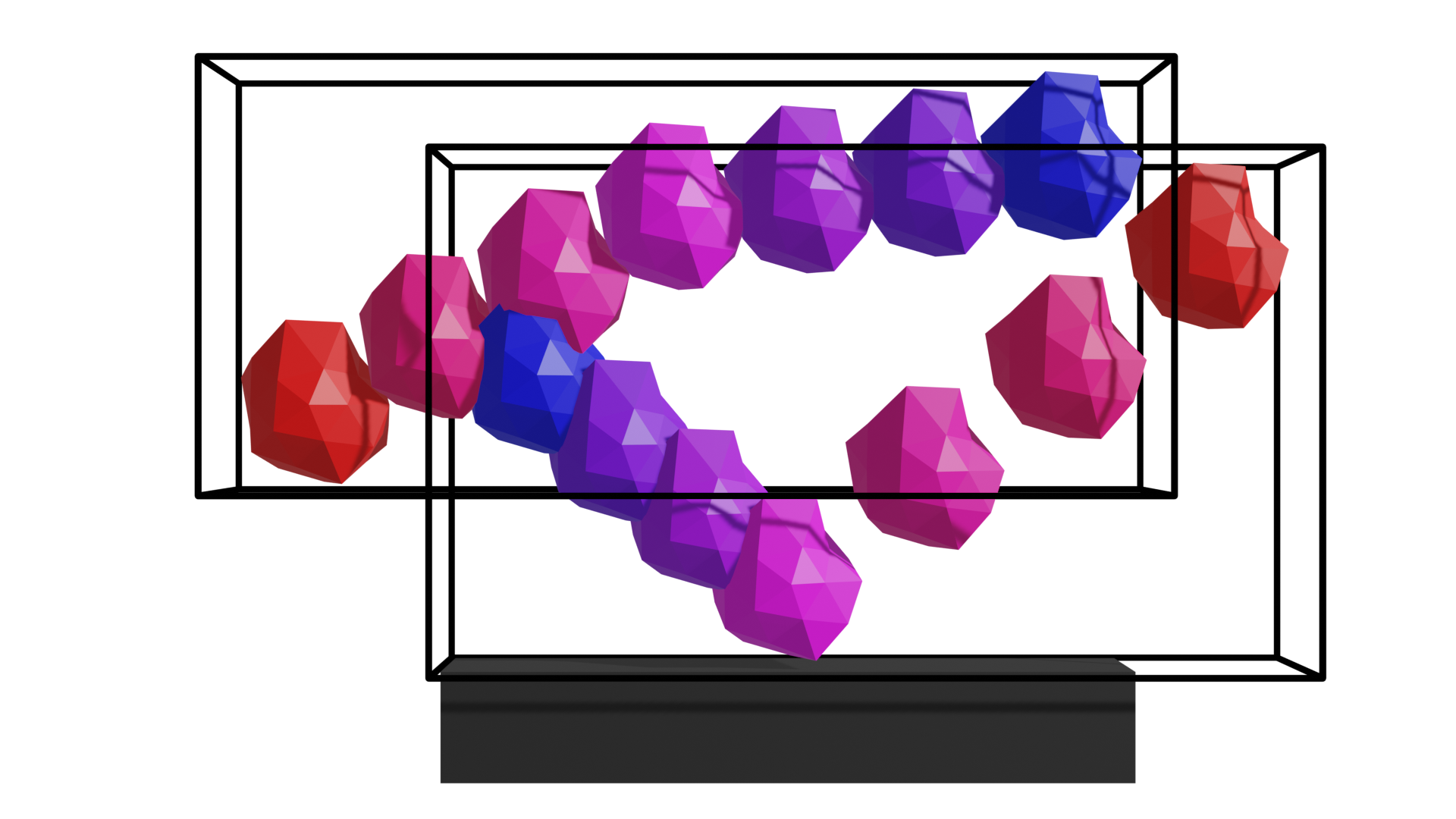
Check 1: Space-time bounding boxes.
With a well-defined time step size per particle at hand, our first technique to construct uses axis-aligned bounding boxes for and constructs a space-time bounding box for . These space-time bounding boxes between any two particles are compared.
As we use a space-time bounding box, the algorithm can be rewritten as a purely spatial approach. The space-time check collapses along the time dimension (Figure 2): We take the particle positions at and and surround both including their -environment with a bounding box. If this super-bounding box of two particles does not overlap, . The handling of and follows the same pattern.
Check 2: Space-time tubes.
Having two space-time bounding boxes overlapping can result in a lot of false-positives, i.e. potential collisions which are not really confirmed later on. This happens, for example, if two fast moving particles move parallel to each other. The second particle might take the first particle’s position after one time step, while the first particle has moved on meanwhile. To eliminate such false-positives, a second test doublechecks and revises entries.
This second technique embeds each particle including its into a bounding sphere . The space-time object now resembles a hose with two linear segments, as we model each particle as a sphere moving linearly along to and then from to . If the hoses do not intersect, we reset . Otherwise, this second test confirms .
Static geometric objects.
The treatment of static geometry parts requires special attention throughout the clustering: Floors for example are often modelled with few huge triangles (Figure 1). Without special rules, they “couple” all particle assemblies hitting this wall globally, even though the assemblies of particles could be handled as separate clusters. We therefore treat static objects specially:
Definition 3.1.
Static geometric objects are parts of all the clusters which host at least one particle which directly interacts with them. However, their collisions do not feed into the cluster identification.
Efficiency, contextualisation and implementation.
The implementation of the two-step check to compute has to be fast. Our realisation relies on Intel Embree’s raytracing kernels [5]. This raytracing software is tuned to handle bounding box checks and variants thereof efficiently. For the actual clustering, i.e. the identification of unconnected subgraphs, a parallel iterative method is used: Nodes are repeatedly coloured with the lowest colour id of their neighbours plus one, until a further iteration produces no changes anymore.
The first pre-check with cubes stands in the tradition of pessimistic algorithms, and yields information of limited interest if particles move very fast or over a long time span, while the second step actually takes rapid changes of the trajectory and fast velocities into account. It prevents too many collision pairs to be added to , while the first step handles quasi-stationary setups quickly and eliminates them from further checks.
Stationary objects such as walls are explicitly omitted from the initial clustering. They are invisible to the extrapolation. Once the clustering algorithm has terminated, we replicate all static objects, such that each cluster sees “its own version” of the static object such as a wall. Many particles that hit the same wall in some distance thus tend to end up in different clusters whereas the wall as proper geometric particle in the computation of would merge all of these objects into one big cluster and remove concurrency.
The efficiency of our overall algorithm depends upon the fact if we eventually manage to use as big time steps as possible to reduce the total number of time steps taken. The time span feeding into the clustering serves as natural constraint for the final time step size. A too large span hampers the expressiveness of unless particles are in totally free flight. We hence make is depend on historic data. Particles which previously have used a very small time step size will continue to try out rather small time steps, while others might use a time step size close to . Through , we can control how quickly a previously slow particle approaches the maximum time step and hence steer the “optimism” in the prediction. We use .
The global is in itself a tuning parameter without physical meaning, which controls the optimism of our time stepping. By picking small , we run risk to constrain those particles overly pessimistically which could travel free of any collision over longer time spans. Large however make the checks overly pessimistic and lead to large clusters.
All steps in this first phase yield classic data parallelism (parallel fors), often combined with a Boolean reduction. The individual checks (per particle pair, e.g.) are reasonably cheap such that further inner parallelisation seems to be unreasonable. However, once identified, clusters form independent units of work. We can handle each cluster as an independent task within this step and from hereon. All tasks and data parallelism are realised via Intel’s TBB [25].
Observation 1.
Particle sets that form a cluster can be treated independently from each other from hereon as separate tasks.
4 Cluster setup and consolidation
As we want to advance all the particles within a cluster in-sync, we have to ensure that they all start from the same snapshot. Our clusters are re-determined in each and every sweep. Consequently, a common time stamp for all particles of a cluster is not guaranteed once the cluster identification in Section 3 terminates. We hence determine from (1) and interpolate between the particles’ snapshots to reconstruct a joint, synchronised state. From hereon, .
Further to the consolidation of the particle snapshot, we also assign each cluster a unique
| (5) |
This is a quantity that is used in follow-up steps. It is a restricted value over the cluster fed by historic data of the individual particles.
Efficiency, contextualisation and implementation.
Per cluster, we run through all particles, but each particle is handled independently. It yields a prime example for data parallelism within the cluster task, where we reduce two scalar quantities, i.e. time step size and time stamps.
Observation 2.
Whenever particles change cluster membership, they typically are rolled back in time.
Our cluster consolidation substep corrects overly optimistic time step choices. However, this is not a rollback in the sense that we return to a previous time stamp. Instead, we interpolate, i.e. we only move slightly backwards in time.
As we reduce the time step size of individual particles, we potentially sparsify further. This can lead to situations where a cluster decomposes into several subclusters which in turn increases the concurrency level. We did not find any performance gain from a re-clustering and further decomposition of cluster tasks, and therefore do not exploit this additional increase of concurrency.
We apply a physical simplification as we assume that we can interpolate. Furthermore, the interpolation relies on the assumption that a particle does not experience any collisions between and (cmp. Theorem 2.4).
5 Time step size calculation
The time step calculation identifies the largest time step size with which all particles of that cluster can safely advance without missing out on further collisions. Let denote the time when two particles’ halos intersect for the first time. It is subject to
| (6) | |||||
The following case distinctions feed into the calculation of :
-
1.
If two particles move away from each other, . Particles that separate at do not constrain the collision search.
-
2.
If two particles’ -area overlaps at , . Particles that stick together at the begin of a time stamp (they rest upon each other or move parallel, e.g.) do not constrain the time step size further.
-
3.
For all other particles, we compute the collision time stamp.
With (6), we can update each cluster’s time step or new time stamp respectively:
Geometric model.
Let describe the set of triangles describing a particle . denotes the volumetric extension of its corresponding triangle , i.e. the triangle plus its -environment.
yields a shell object, i.e. a volumetric geometric object into which the surface of the particle is embedded.
Definition 5.1.
A contact point is a tuple of a position in space , a time stamp , a normal vector and two triangles and from two different particles . The following properties hold:
-
1.
The distance between and or is at most .
-
2.
Two triangles have at most one contact point per time stamp.
-
3.
is the shortest distance vector to one of the nearest triangles.
Two particles are in contact at a certain time, if there is at least one contact point between their triangles. We note that two triangulated particles can yield redundant contact points if any contact lies on a shared edge or vertex and thus arises from multiple triangle pairs. Contact points furthermore are not unique for parallel triangles—they can be located anywhere on a submanifold within the -overlap. Our discussion from hereon assumes that contact points are filtered, i.e. contact points that are close in space are fused into one contact point to avoid spatial replicas and are centred within parallel triangles.
Collision time detection.
Contacts between two triangles either are placed on the shortest distance between a vertex of one triangle and the other triangle’s surface, or are located in-between two triangle edges. Efficient code blocks to compute them are known [18, 11]. We have to transfer such spatial algorithms into the space-time domain over with a new (minimal) in-between to be determined. For this, we employ an iterative algorithm.
Definition 5.2.
We compute an effective time step size (cmp. Definition 2.2) from by reducing this time span until any further reduction of the time step size would yield no collisions within the cluster. This process is called narrowing.
We realise the narrowing iteratively by repeatedly reducing the time span in which we search for collisions. Per iteration per triangle pair, we treat vertex-triangle and edge-edge comparisons separately: For each vertex-triangle pair, we compute the position of the vertex relative to the triangle at the begin and end of the maximum admissible time step: We use a relative coordinate system which moves with the triangle. After that, the algorithm takes the space-time line segment connecting the two relative positions. We can now analytically compute the minimum distance, as the minimum distance is either observed at the start or the end point, or arises from the time stamp when the line intersects the (relative) plane in which triangle lives—if it exists. For each of these two or three, respectively, situations we can use Barycentric coordinates to construct the actual contact point plus its time stamp. It is an approximation as we neglect rotation. For the edge-edge comparisons, we lack an analytic formula and hence sample the initial distance, the final distance and the distance in-between. Both types of distances might identify a contact with a certain time stamp. As long as the minimum of these contact time stamps remains smaller than the time span of interest, we narrow the span just to include this minimum and rerun the tests.
Accelerated multiscale algorithm.
To accelerate this narrowing, we use an iterative multi-resolution scheme exploiting the notion of surrogate geometries [18]:
Definition 5.3.
Let a surrogate representation of a triangle set be another triangle set with
| (7) | |||||
| (8) |
The in (7) is the parent of its corresponding .
Per particle, we hold a sequence (levels) of surrogates , . Each surrogate is conservative with respective to the next finer surrogate due to (7): If two surrogates of level do not collide, their corresponding surrogates of level do not collide either. Each surrogate is also effective with respect to the next finer surrogate due to (8): It is cheaper to handle a surrogate of level compared to the surrogate of level , as the former features fewer triangles.
As (7) formalises a surrogate tree, we can introduce an efficient multilevel iterative variant expanding upon our vanilla code version:
-
1.
For two particles , of interest, we start with their coarsest surrogate representations. They define the search sets and .
-
2.
Per pair , we approximate the minimum time of contact. and are removed from their search sets once we have evaluated all the pairs they are involved in.
-
3.
If a new contact times exists and it falls into our search span defined by and ,
-
•
we update if they reduce this quantity further and if and are both taken from the fine mesh triangulations, i.e. ;
-
•
otherwise, we throw away these contacts and the contact times and instead insert all children of and into or , respectively.
-
•
-
4.
If , we continue with Step 2.
Efficiency, contextualisation and implementation.
Our particle-to-particle comparison only studies particle combinations with . Even though two particles reside within one cluster, we might have come to the conclusion earlier that these particles cannot collide. This information is used here.
Within each particle-particle comparison, the multiscale variant terminates the exploration of branches of the surrogate trees early. Even triangle pairs that would result in a collision later within the search time span are omitted, once we know that another triangle pair yields a collision earlier on. We reduce the number of triangles to study within the tree, but also decrease monotonously. Therefore, it makes sense to study all first levels of all particles within a cluster first, before we switch to the next finer resolution for further geometry checks. For this later unfolding, we might already have reduced and hence study fewer triangles from the second resolution level.
We assume that triangles move linearly through space. This is not valid once . Our current implementation ignores the possibility that a section of an object rotates fully through another one. For small admissible time step sizes and slow rotations, this is reasonable. In an application with finer interacting geometry (for example, fine teeth on interlocking gears) it may be necessary to add extra checks here. An alternative option is it to increase the region of each triangle and surrogate to ensure the real volume swept by a rotation triangle is covered. Notably, we can make the larger the coarser the surrogate. While this would introduce more false-positive collisions early throughout the multiscale algorithm, it would ensure there are no false-negatives. More sophisticated geometric methods exist [28] which might be able to provide additional efficiency and correctness guarantees for such challenging cases.
Experimental evidence suggests that floating point round-off errors lead to situations, where the algorithm yields no contact points at all, as we just slightly underestimate a valid . Further to that, we will need a certain non-zero overlap of the particle s in the subsequent step. Therefore, we make our algorithm artificially increase the time step size slightly after each iteration This is admissible, as we work with weakly compressible objects subject to an -layer anyway. Inspired by static code analysis in Definition 5.2, this slight increase of the time step size should be labelled widening.
Observation 3.
Even though we search for a minimum contact time per cluster, multiple contacts can arise.
The algorithm’s underlying sweeps over particle pairs and triangle pairs translates directly into data parallelism. However, a realisation with parallel for loops over the surrogate levels is disadvantageous as it introduces synchronisation points after each level. It also suffers from non-constant compute cost per compute step. We hence advocate for a strict dynamic task tree formalism, processing triangle-triangle pairs within the surrogate hierarchy independently. The unfolding of this task tree is constrained by a global (atomic) contact time, i.e. we might unfold too many tree nodes.
6 Particle interaction
Our physical model approximates both the instantaneous collisions between particles both temporarily and spatially (Observation 3). Any overlap of the -layers is considered an immediate contact [10] and feeds into a hard “sphere” model with a perfectly ellastic collision, which we can damp due to material laws. Let denote all contact points within a cluster, and let identify the two particles associated with a contact point . We end up with a constrained equation system for the exchanged impulse
where is the normal of the contact point , denotes masses of the involved particles, the acceleration and the particles’ velocity. We solve for . The arising s depend on the accelerations from all the contact points plus the incoming velocity as well as the time step size chosen.
The constraint phrased over the outgoing velocity makes the scheme implicit. Due to it, particles stop approaching immediately as soon as they get in contact. As our time step size is fixed at this point, we can disregard the mesh, argue solely about the set of identified contact points, and consider each particle to be represented by a current and future transformation resulting from this set of contact points.
This is a non-trivial, non-linear equilibrium equation system due to the constraints. We apply a Picard iteration to solve it, where we update the individual contributions per contact point one by one. The constraints are weakly enforced via a penalty term, and we damp the iterations’ updates using linear combinations of previous and newly computed solution guesses. In line with other codes, we assume that the Picard iterations converge [21], which is reasonable as we minimise such that only few contact points remain.
Since the constraints are phrased over relative velocities and not on the lengths of the contact normals, we can end up in a situation where particles gradually drift towards each other over several time steps, even though their relative velocity is canceled each time they come into contact. They might be pressed closer and closer together by other particles in the system. Eventually, they might even start to penetrate. This happens notably once large stacks of objects settle into a pile of particles on the ground.
Therefore, we add an additional force term to slowly separate the particles. This artificial term does not contribute to the resulting velocities. Further to that, we use a simple Coulomb friction model where an impulse is applied along a tangent to the contact normal to reduce the sliding velocity. This impulse is bounded by the impulse along the normal multiplied by the coefficient of friction between the surfaces.
Efficiency, contextualisation and implementation.
An alternative, popular force model replaces the Dirac force distribution with a smooth force function. Its support is bounded by , i.e. it is zero if the distance between two objects or triangles exceeds , i.e. their contact point carries . Finally, the contact force , as the distance becomes smaller and smaller. The smooth approximation of the force function means that particles become weakly compressible, and their interaction resembles the compression of a spring. We employ this model in our previous work [18].
The present approach also can be read as an approximation of the force. However, instead of embedding a smooth force function into the -area, we employ a heavyside function which jumps to a constant value at the point that we identify as collision time stamp. It is the magnitude of this function which dynamically adapts to the state of all particles. It is hence an semi-implicit formalism of particle collisions: the position updates continue to be handled explicitly, the arising forces aka accelerations are integrated implicitly. As we solve the arising equation system (and add an artificial spring term), we have a conservative physical model which ensure that we never run into unphysical solutions. Overall, this part of the scheme is similar to an event-driven simulation [17].
The whole contact resolution is non-trivial to parallelise effectively without fundamental changes to the algorithm. Locks or atomics for example allow us to update all particles involved in contacts in parallel within the Picard iteration. Our experiments with these techniques however showed a drastic decreases in performance. We instead colour the per-cluster graph and update those particle’s momentum in parallel which do not simultaneously feed into other updated particles. That is, if there is a collision between and and and , and are updated in one rush, while is updated afterwards. This bounds the concurrency of the implementation yet outperformed alternative trials.
While we note that clusters can still be updated in parallel in this phase, we note that the cluster masking in (2) effectively disables most clusters from processing. The concurrency level resulting from multiple cluster is limited.
7 Efficacy and correctness
The proof of Theorem 2.4 is technical yet brief with a combination of an induction over the number of particles plus a contradiction. As we terminate our algorithm as soon as the global time stamp exceeds the terminal time, the theorem states that the simulation outcome is correct.
Proof 7.1.
The correctness is trivially true for one particle.
Let all state transitions be globally enumerated. We use the counter for the enumeration. Assume that the tuple produced for particle in step is invalid: it should not have been made, as we dropped an old solution in this step to which we should have rolled back. This formalism implies that step triggered the state transition
By induction, we know that and that it has been particle which would have crashed into at a time . This is the collision we missed.
and have been in different clusters in step . Otherwise, they would have advanced in sync. Therefore, there is a step in which has updated its position the last time.
from thereon, i.e. we haven’t updated this particle anymore since then. According to our assumption, we learn about this missing collision after step , but the actual collision happened at . Now we cannot roll back anymore. This can happens if and only if particle lacks behind.
’s transition in step is allowed if and only if the other particles in their clusters have not been left behind. Otherwise, we violate (2). This is a contradiction to the time constraints on above.
Theorem 2.5 rephrases that after a finite number of time steps. With a detailed description of the individual algorithmic steps, we can indeed show that our algorithm terminates.
Lemma 7.2.
The time step sizes of active particles are significantly bigger than zero, i.e. they do not deteriorate.
The lemma can only be proven once we assume that the kinetic energy of a system is not growing, i.e. as long as the system is closed and no energy is injected.
Proof 7.3.
Let a particle that is not subject to changes of its kinetic energy follow a trajectory of straight line segments . This is the analytic trajectory, i.e. no two line segments point into the same direction. To contradict the lemma, . Such a situation can arise if a particle, for example, falls into a funnel or hopper and bounces in-between the walls coming closer and closer, until the particle finally gets stuck in-between walls.
We first recognise that the reduction above means , as our particle interaction model is subject to friction. A particle notably cannot bounce forth and back between two walls without slowing down.
However, to construct such a trajectory is not possible for our algorithm, as the particles are surrounded by an -layer. Hence, the segment length is bounded by or two particles are in a “permanent” contact, i.e. stick to each other. In the latter case, the interaction is explicitly removed from the time step size calculation.
The lemma formalises the in (6). It becomes clear that friction works in our favour in this context: As particles slow down due to friction after each collision, even constant path segments would lead to larger time intervals in-between collisions. Even without friction, our -formalism effectively truncates analytical trajectories of line segments which would approach zero. One can still construct arbitrary long sequences of time step sizes approaching zero if a system is permanently stimulated by injecting additional kinetic energy. We neglect such setups.
Observation 4.
The semi-implicit collision model, where the contacts are prescribed and only impulses are implicitly determined avoids time step size degeneration and bouncing particles when we encounter compact, settled particle geometries.
With a smooth spring force, time step sizes have to be dramatically reduced as long as two objects continue to approach each other despite the actions of the force. As a consequence, global assemblies of objects with multiple contact points will rarely reach an exact equilibrium. They will always oscillate around the steady state solution as long as an external force such as gravity holds them together or otherwise disassemble. While a force-based formalism may have its advantages, such vibrating assemblies of objects are problematic for local time stepping, as they lead to an effective time step size degradation. It is hence not only an algorithmic decision to determine the contact points and impulses implicitly each—though the overall schemem remains explicit as these to ingredients are not coupled—but it is essential to make the local time stepping work.
Lemma 7.4.
The particle with the smallest is always a member of an active cluster.
Proof 7.5.
We assume the lemma were wrong an construct a contradiction: Let , i.e. let determine the global minimum time stamp. Another particle carries . Let and end up in different clusters, were they both determine the minimal cluster time stamp or respectively.
If vetos the advance of the ,
However, by definition.
What could happen however is that cluster takes a large time step and overtakes the particles within , missing out on collisions at . In this case, it will roll back later to as particles from and are joined into one cluster.
Lemma 7.6.
Every particle is updated after a finite number of steps, i.e. every particle becomes a member of an active cluster.
Proof 7.7.
The lemma (and proof of Theorem 2.5) results directly from the previous lemmas: A particle is not strictly advancing in time. However, let be a sum over all particles with . This sum is strictly monotonously decreasing with a decrease that bounded away from zero. After a finite number of steps, particle is therefore updated.
8 Runtime results
All experiments were run on AMD EPYC 7702 chips in a two socket configuration with cores. Each socket is divided into 4 NUMA regions. Our code was translated with the Intel oneAPI C++ Compiler icpx 2021.4.0 using the flags -std=c++17 -O3 -march=native, i.e. we tailored it to the native instruction set. Our realisation relies on CGAL 5.5.1 [27], Eigen 3.4 [4], Embree 3.13 [5], libigl 2.3 [16], SIMDe 0.7.2 [22], TetGen 1.6.0 [26], Catch2 3.1.0 [1] and GLFW 3.3.6 [7]. As our prime interest is runtime, we hardcode key geometric properties: is uniformly used unless specified differently, and the Picard solver for the particle interaction steps considers an estimate of the momentum exchange as converged when the update to the impulse and torque applied to every contact underruns a threshold of .
We always benchmark our local time stepping against a global approach. The latter uses the same software architecture, i.e. works with clusters, an implicit momentum exchange and per-cluster collision timestamp identification, too. To make it a globally adaptive scheme, we use (2) to constrain all time step sizes: Clusters identify their effective time step size, but then reduce it further whenever another cluster identifies that it can only advance with a smaller one. This mirrors textbook adaptive global time stepping. Due to the damping of the time step size in (3), a locally stiff collision implies that all particles in the stimulation adopt a tiny time step size. Besides this additional constraint—which can be read as an explicit further narrowing of the time step size per cluster once the time step size calculation has terminated (cmp. Definition 5.2)—the global time stepping code equals excactly the local version. Notably, it exploits the same parallelisation techniques and hence provides a fair comparison baseline.
8.1 Particle pairs
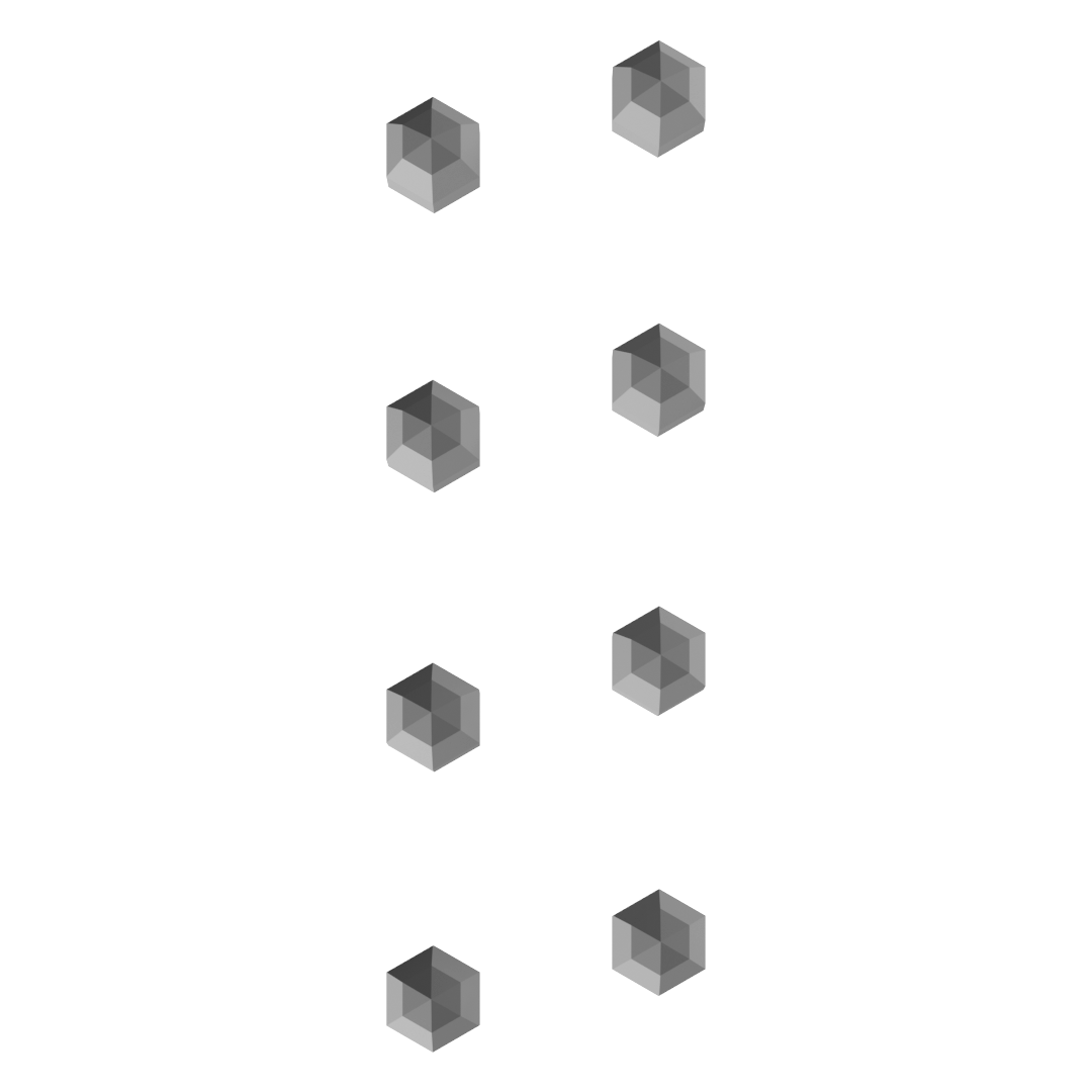
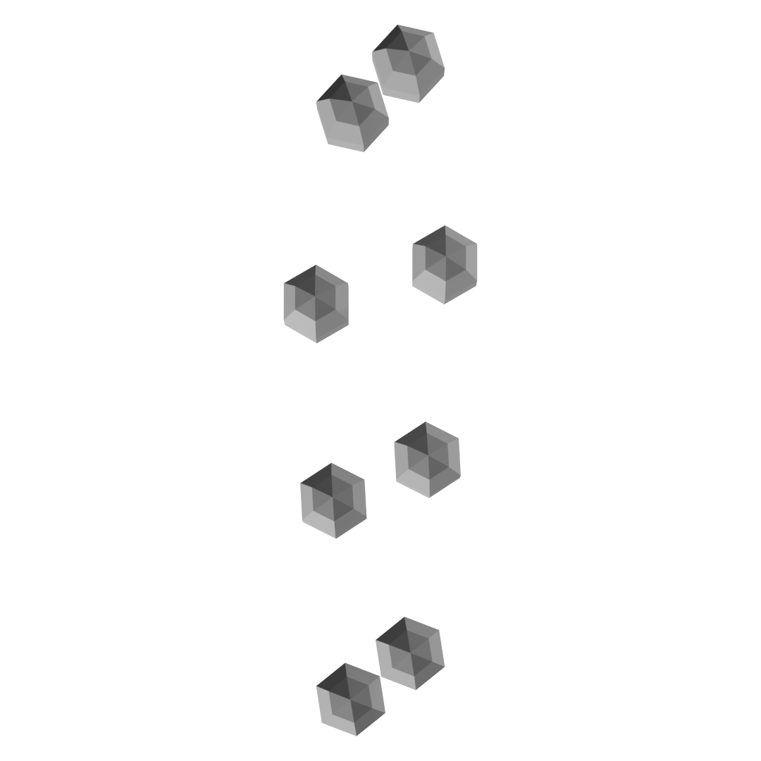
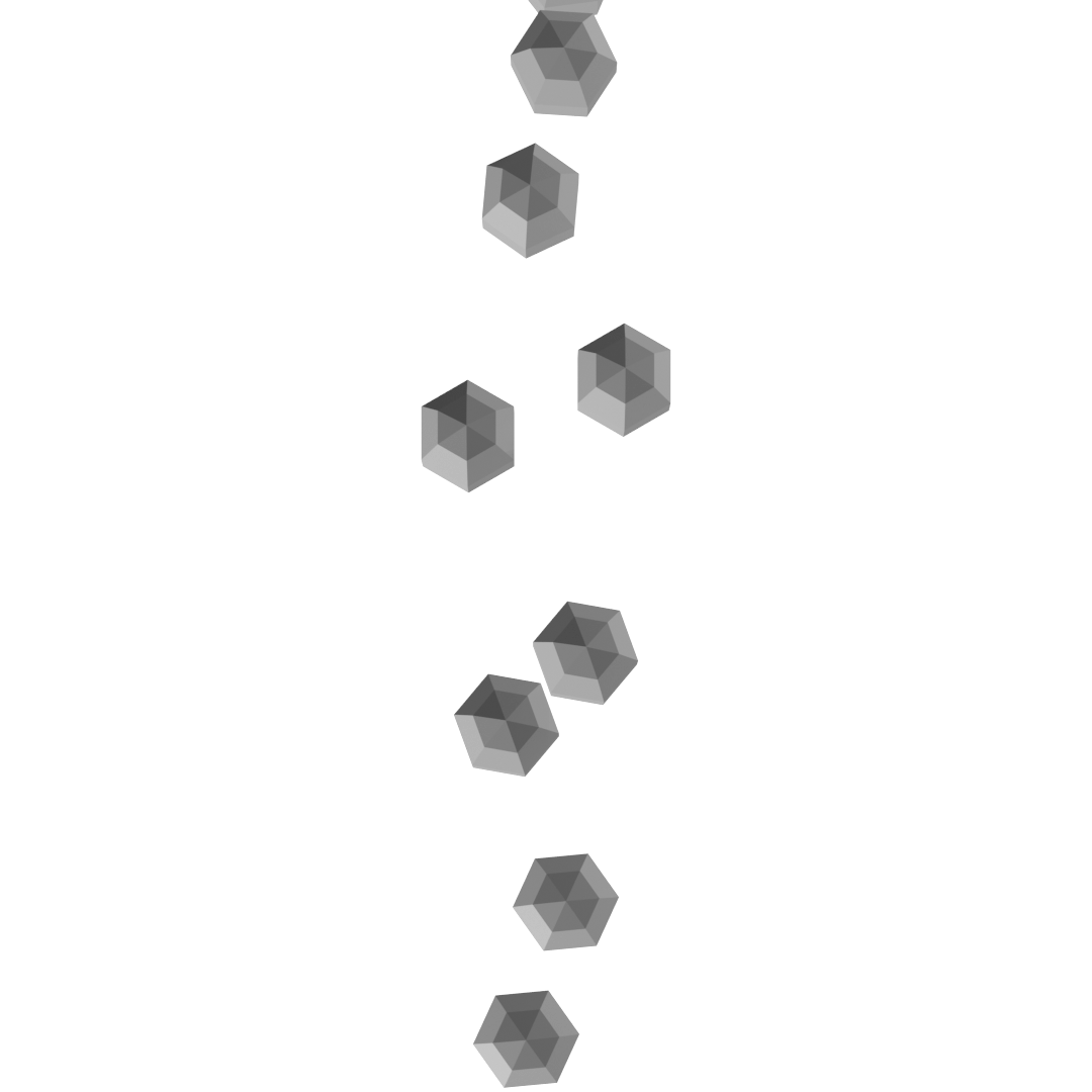
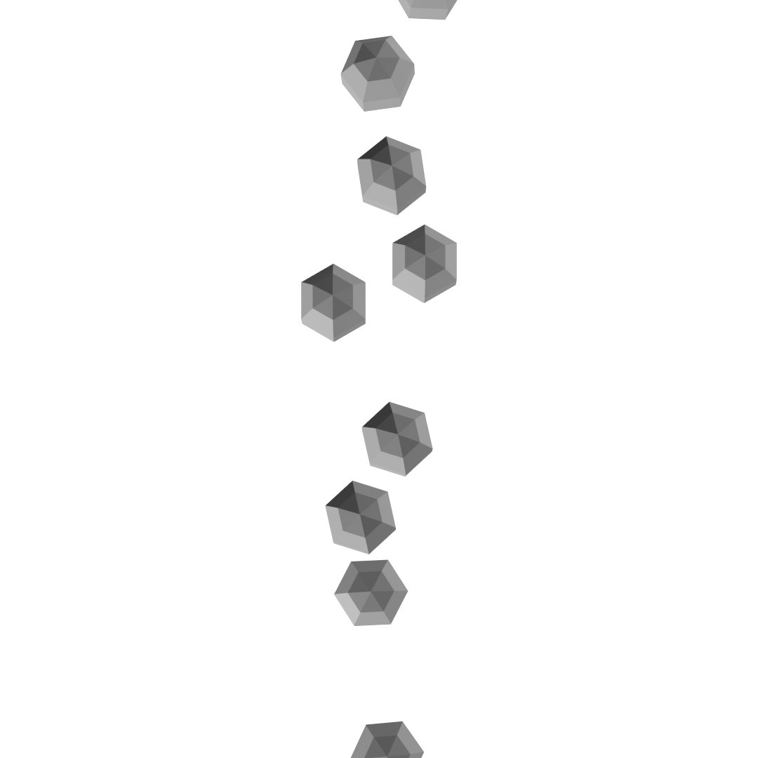
In a first experiment, we create two sets of particles. Both host the same number of particles, which are arranged vertically yet spaced out. They do not touch each other (Figure 3). The particles used are of identical size, spherical, and we use and .
The two sets are put next to each other like columns. The two columns in turn are set on a horizontal collision trajectory, such that always two particles bump into each other. As we randomly vary the initial horizontal velocity magnitude per particle, the collision time stamps differ. We configure the initial geometric arrangement of this particle-pairs scenario such that each particle collides exactly once with its counterpart.
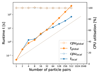
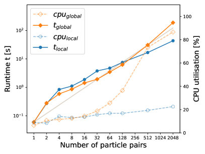
Each particle pair runs through three computational phases: While the particles approach, there is no collision and no forces act on the particles, as we omit gravity. When they collide, the system becomes very stiff suddenly and the particles exchange forces. When they separate again, there are no forces. As we use random initial horizontal velocities, the phases of the different particle pairs are not synchronised in any way.
Observation 5.
On both a single core and on multiple cores, local time stepping outperforms global time stepping for the particle-pair setup as soon as we accommodate sufficiently many particles. It scales close to linear with the number of particles, while it underutilises the available CPU resources.
Cluster topology, active clusters and concurrency level.
Tracing of the algorithm’s internal states provides insight into the runtime behaviour (Figure 4): The algorithm observes a maximum cluster size of up to five particles. This is up to 2.5 times worse than the theoretical optimum, as we know that at most two particles at a time should be member of one cluster. As the particle pairs are totally out-of-sync, the clusters “diverge” in time quickly. Due to the global constraint (2), this leads to a situation where only few clusters can be updated per time step. We obtain a low CPU usage (below 25%).
| Phase | Run time | Run time | Run time |
|---|---|---|---|
| 64 pairs | 512 pairs | 8192 pairs | |
| Broad collision | 0.9% | 0.5% | 1.0% |
| Clustering | 0.2% | 0.2% | 0.7% |
| Time step size | 82.6% | 83.0% | 82.7% |
| Narrow collision | 16.2% | 16.0% | 15.0% |
| Collision | 0.2% | 0.2% | 0.6% |
| Snapshot roll-over | 0.0% | 0.1% | 0.0% |
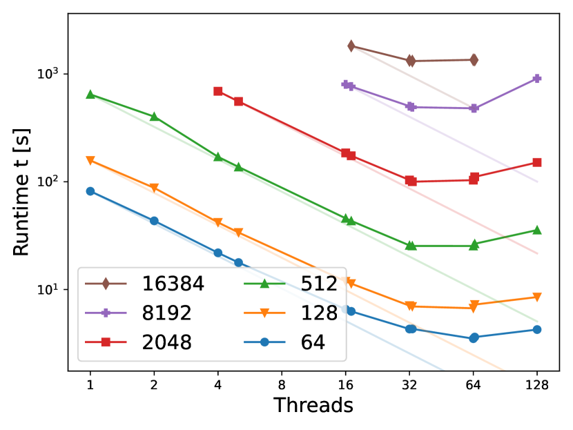
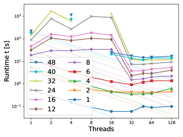
Despite the low CPU utilisation, we get reasonable weak scaling (Figure 5). Since we know that the clusters all hold similar particle counts (usually two), we have to assume that there are few active clusters per time step, yet usually more clusters than we have numbers of cores. Furthermore, the data suggests that the number of active clusters per time step scales almost linearly—the weak scaling is not perfect—with the number of total particles.
Time step size distribution.
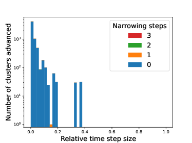
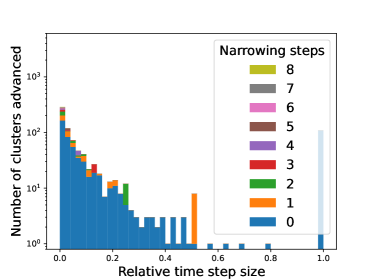
We initialise our simulation with a global threshold which is equivalent to the mean time span up to the first collision in the system. For the global time stepping, at least one particle pair will collide slightly earlier than that, i.e. we immediately reduce the effective to a fraction of the original choice. The next few steps reduce the time step size further, as more and more particles crash into each other (Figure 6).
Local time stepping allows some clusters to advance with the maximum initial . The time step size histogram hence shows entries for the relative time step size of one. After the first particle-pair has collided, other particles continue to collide and to “bounce back”. The time step size histogram fans out due to (3).
Since the time step size is aggressively reduced immediately by the global time stepping, very few narrowing is required. The local time stepping in contrast requires narrowing. At the same time, the number of cluster updates with the tiny time step sizes is by magnitudes smaller than for global time stepping, and we see a more “spread out” distribution of the used time step sizes. This explains the good performance of local time stepping compared to its global counterpart.
Contact points and particle interactions.
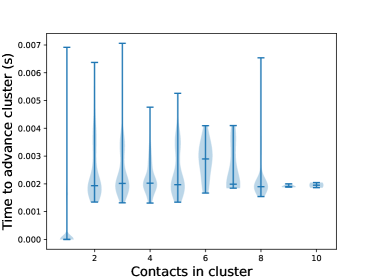
Up to ten contacts are found per cluster, i.e. particle-particle interaction. Most of the time however, particles collide only in one single point. The implicit momentum calculation hence becomes close to trivial. The time step size calculation dominates the runtime (Figure 5).
Discussion.
For small particle counts, we obtain a superlinear cost curve relative to the particle cardinality. It is not clear if this is due to caching effects—as we add more particles, they might “fall out close caches”—a significant management overhead, or a combination of both. As the particle count increases, any overhead is amortised, and the local time stepping cost curve starts to approach a linear trend. Parallelisation subsequently helps to reduce both the curves’ growth.
Our setup is of artificial character. However, we note that many subsequent experiments lead to small particle groups “spinning off” from the main bulk of the objects. As they fly away, our cluster analysis manages to find out that they barely interact, packs them into their own cluster and handles them in parallel. Even if a light, fast particle crashes into an assembly of compact objects, we see that the local time stepping can handle this situation efficiently.
The setup also uncovers one further detail: The cluster masking prohibits particles to “shoot off” into the future after their first contact, since the algorithm is unaware that particles collide at most once. However, additional domain knowledge such as “this particle is shooting away” would permit us to disable the time step size constraints for the particles. We could evolve them straight to the terminal simulation time and hence reduce the compute cost further.
8.2 Particle stacks and the tower setup
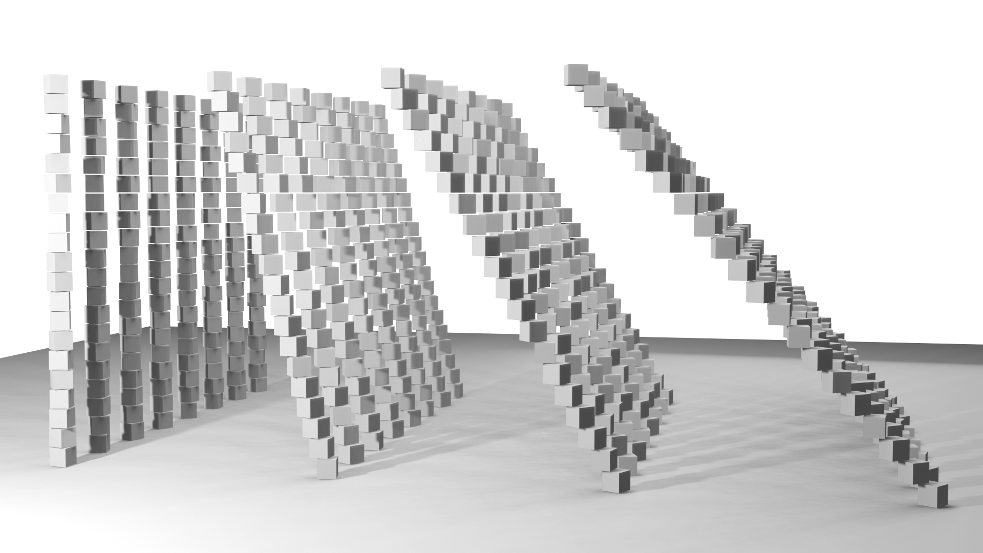
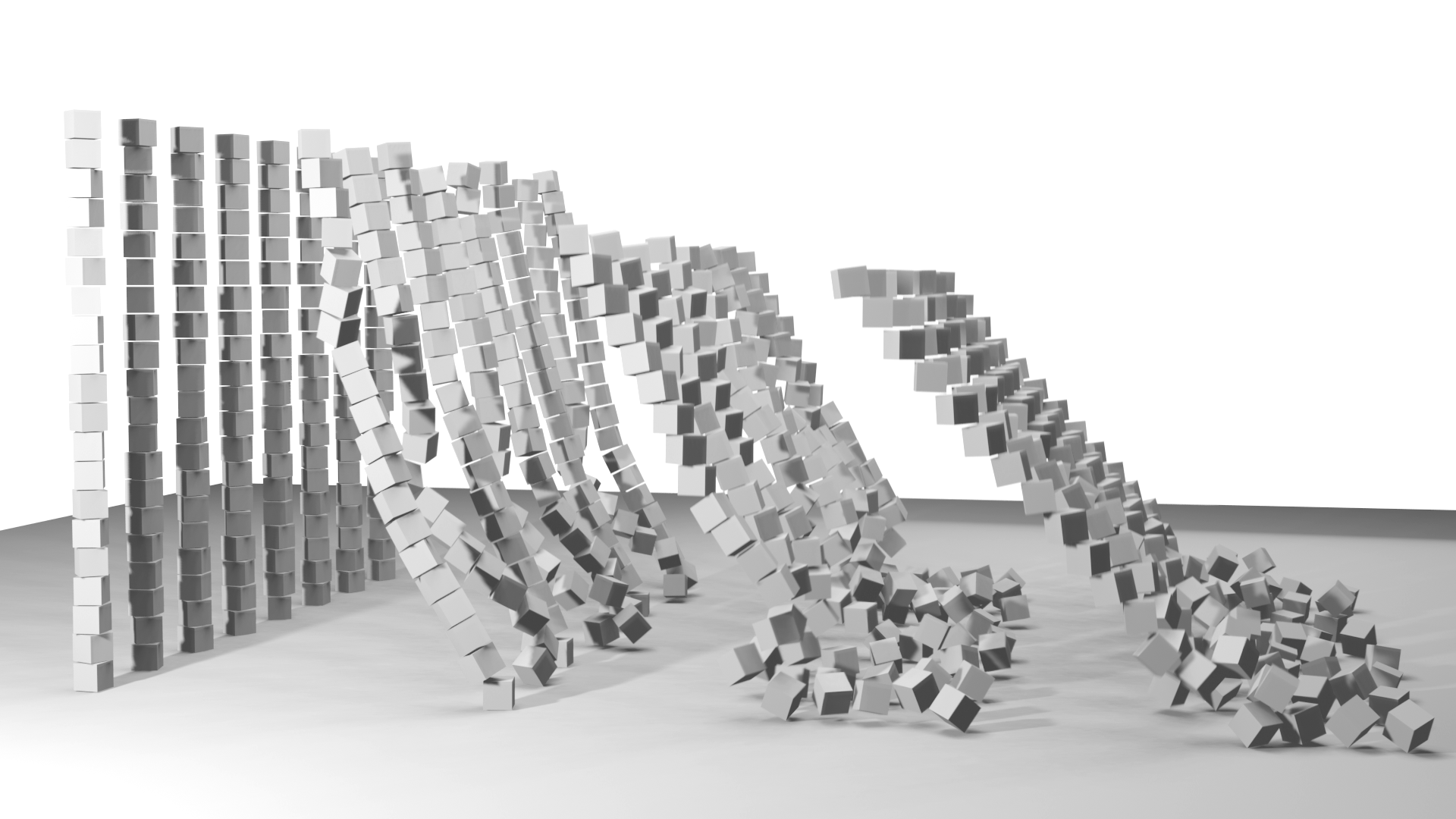

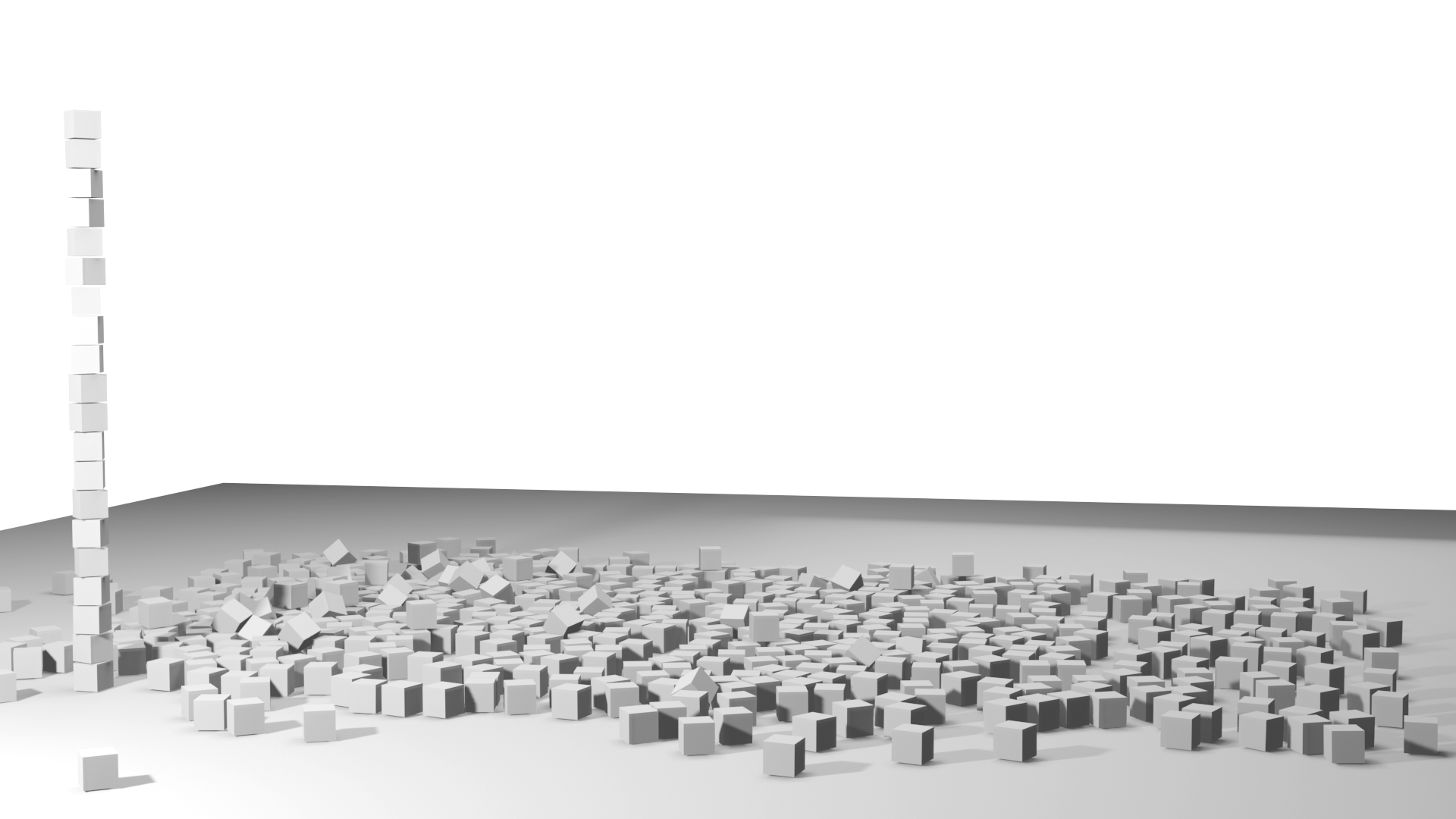
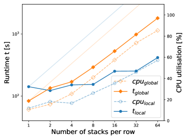
In a second setup, we study a series of stacks of cubes which are initialised with a variety of slanting angles. The stacks are arranged in a Cartesian layout. As all but the left-most stacks are unstable, each stack topples over and interacts with the other stacks (Figure 8).
Again, our simulation progresses through three distinct phases: Initially, the particles aka cubes form stable clusters. They stiffly interact with their adjacent cubes only. In the second phase, cubes crash into cubes from other stacks or cubes from their own stacks before they distribute over the floor. In the third and final phase, the cubes “roll” over the floor before they finally come to rest.
In our simulation setup, the ground plane is modelled by two triangles, and the cubes use . We scale the setup by increasing the number of rows of stacks, while we always employ 20 cubes per stack and four stacks per row.
Observation 6.
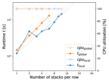
Except for small setups with very few stacks, local time stepping outperforms the global time stepping approach on a parallel computer.
Cluster topology, active clusters and concurrency level.
As long as the particle stacks remain more or less “intact”, i.e. while they tilt, we obtain around one cluster per stack. This is due to the fact that the stationary floor is explicitly excluded from the cluster construction. Once stationary, we get many clusters consisting of few particle, as particles end up scattered over the floor. In both situations, local time stepping manages to advance the clusters aggressively.
In-between these two phases, the cluster topology is quite dynamic. It is this in-between phase, where the overall system is rather stiff and employs small time step sizes. However, individual subclusters of particle constellations might nevertheless advance aggressively in time; notably when they have not yet crashed into other pillars or have already come to rest. Overall, we see the local time stepping outperform a global time stepping once the particle count is sufficiently high, and we even have superlinear scaling in the number of particles (Figure 9).
Time step size distribution.
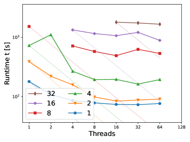
At the same time, this frequent change of cluster topologies implies that the scalability is not particularly good. This observation is independent of the total particle count (Figure 10). At any point in the intermediate phase, many particles either are associated with inactive clusters, may have to roll back in time, or may only advance with tiny time steps. Therefore, the algorithm struggles to benefit from additional cores.
Contact points and particle interactions.
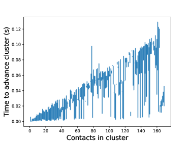
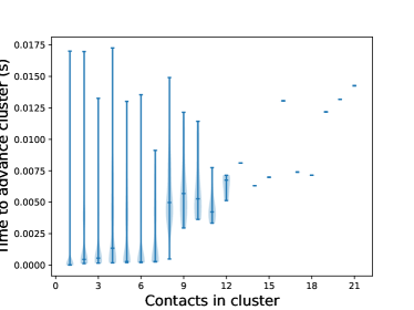
In the first and third simulation phase, particles on average experience either one or two contact points. The solution of the arising non-linear equation systems is rather straightforward. In the expensive middle phase, some particles face many stiff contacts within a single time span. The arising equation systems become larger and (potentially) require more iterations. We end up with a linear correlation trend between the number of contact points and the cost to solve the arising system (Figure 7). The coincidence of expensive contact resolution with phases of low concurrency explains the limited weak scalability.
The tower setup.


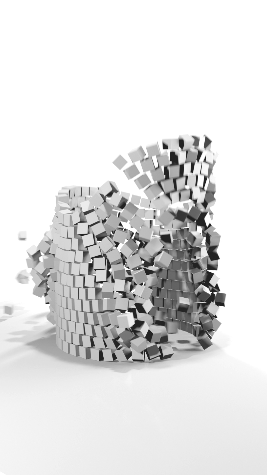

We confirm our observations through the particle-tower setup, where we arrange rings of 32 cubes into layers on top of each other. Similar to bricks, they yield a tower-like construction. A small, heavy and very fast moving object crashes into the bottom of the tower and makes it collapse (Figure 11).
Initially, the tower is in a steady state. Its bricks (particles) do not move. As the projectile hits the tower, a shock travels through the structure as the particles are incompressible. Cubes in the tower use , the ground plane uses and the projectile uses . We scale this experiment by increasing the height of the towers.
Observation 7.
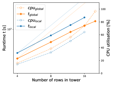
The tower yields a computational character that is an extreme case of the stacks: Two clusters “suddenly” interact and the simple two-cluster topology is completely destroyed, before the simulation settles.
With a dense packing of the tower bricks, the setup is either (almost) at rest or the shock has separated off particles already. Compared to the particle stacks, we have a simpler topology, and this topology remains intact over a longer time span. Therefore, the CPU usage of the local time stepping follows the global one, and we get close to no scalability (Figure 12). As we only enrich one cluster with more and more particles, we see a linear increase of the compute cost for both local and global time stepping. For reasonably large setups, we gain performance once we add a second memory controller; which is stereotypical for bandwidth-bound codes.
Just after the single projectile particle has hit the tower, we obtain very small time steps and the tower’s cubes hence decompose into various clusters. At this point, clusters start to advance with slightly differing time steps. However, the geometric topology changes again, particles are rolled back and we hence do, compute time wisely, not benefit from the arising concurrency.
Discussion
Our algorithmic design is guided by the geometric identification of clusters. If such a cluster topology ceases to exist, we can not exploit a spatial decomposition anymore to obtain a scaling code. We also loose the opportunity to march different particles in time at different speeds. It is reasonable to assume that composites of many particles require a different algorithmic approach compared to the techniques presented in the present paper. Notably, it makes sense in such a case to work with larger, globalised clusters and hence to avoid any overhead imposed through local time stepping.
8.3 The hopper and the staircase
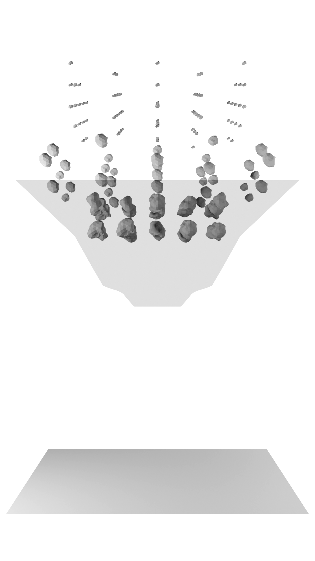
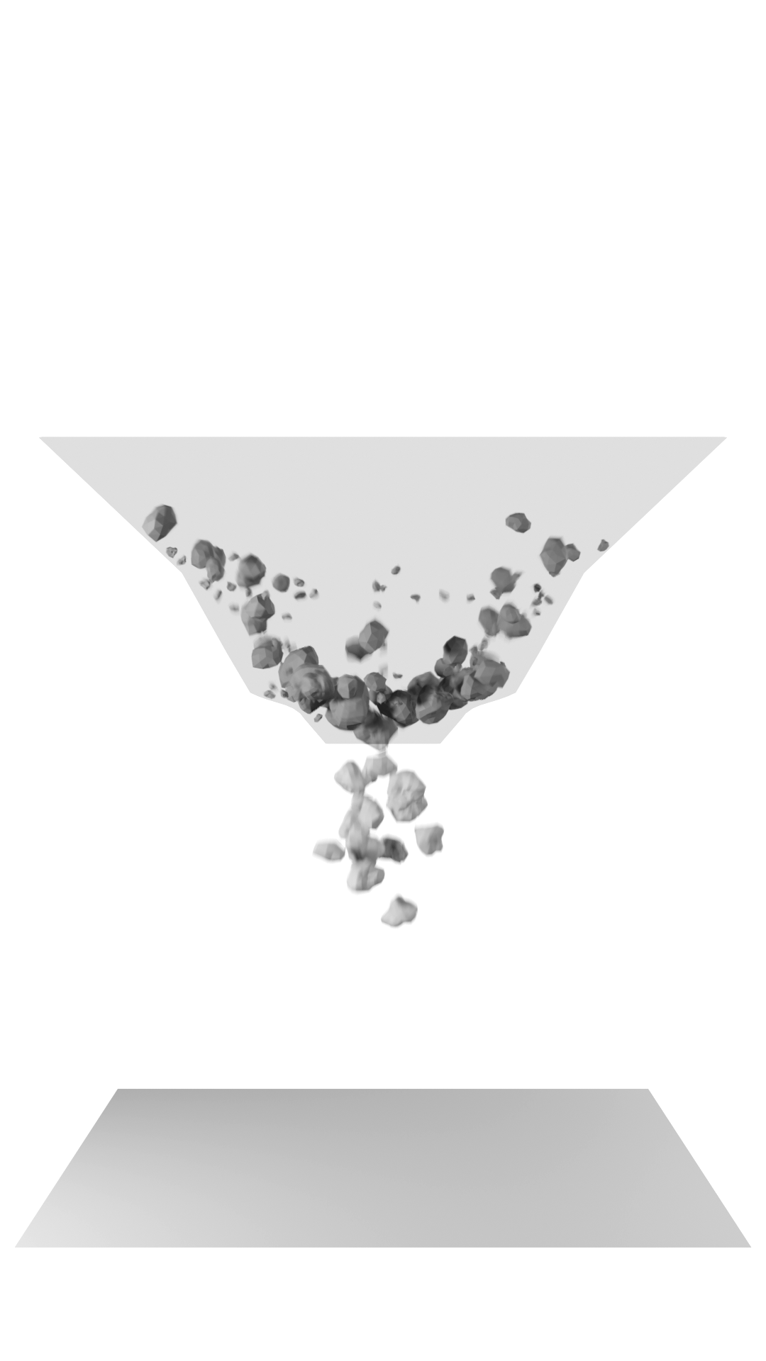


We close our experimental studies with two sophisticated setups: In our hopper scenario, a collection of particles is dropped through a hopper and comes to rest in a pile on a plane underneath. Dropped particles begin in free fall with no interaction with surrounding particles before they enter the hopper. As they bounce from the hopper walls, and as more and more particles fall into the mouth of the hopper over time, they interact both with each other and the hopper’s walls (Figure 13). Our hopper model consists of triangles and its opening at the bottom can accommodate around four of the largest particles at the same time.
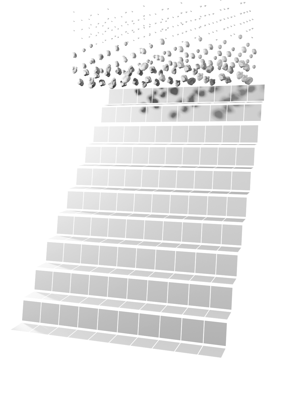
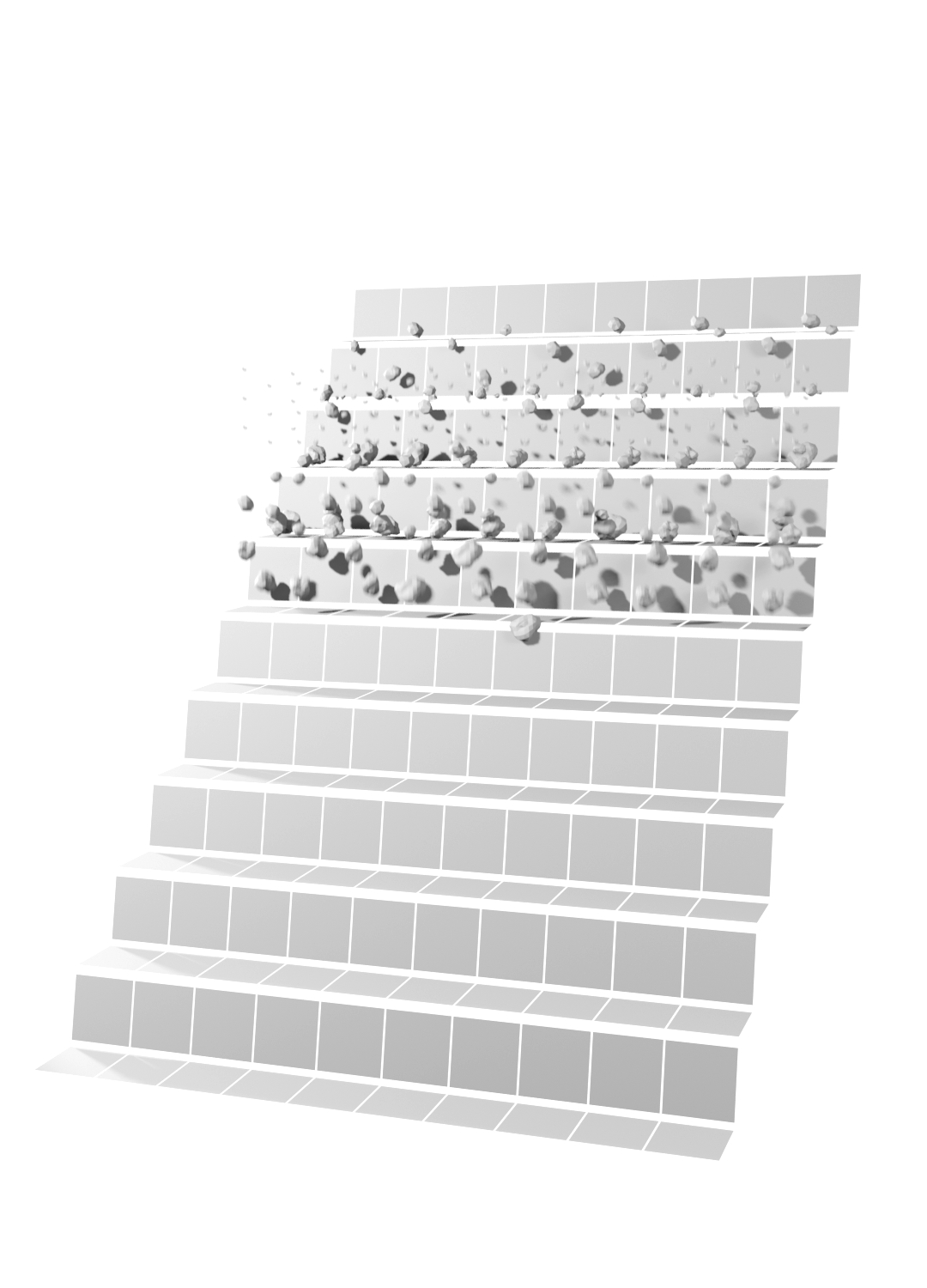
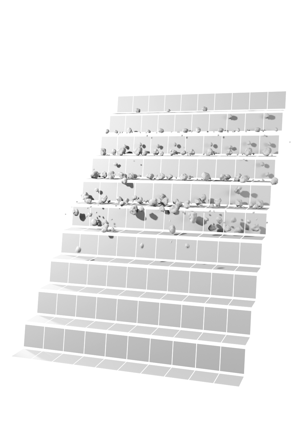

In our staircase setup, we let the particles hop down a staircase (Figure 14). The staircase is made up of 20 planes, each consisting of two triangles. Whenever particles hit the staircase, they either come to rest at their step or continue toppling downwards. They can hit further particles and knock them off their respective steps where they might have come to rest already. Eventually, all particles are either settled on the flat steps or have fallen over the side or bottom.
In both scenarios, we use sphere-like, triangulated particle shapes. They result from a triangulation of a sphere subject to random, hierarchical noise: We decompose the sphere equidistantly into triangles. The distance of the triangles’ vertices on the sphere is added Perlin noise, which offsets the vertex along the normal direction of the surface.
If is the radius of the original sphere, we end up with distances from , i.e. adds no noise and thus yields a perfect, triangulated sphere. The higher the more “degenerated” the particle featuring both low and high frequency geometry distortions on the surface. Manipulating and , we randomise the size and shape distribution of the particles [18].
The quasi-spherical particles range from small grains ( and a radius of ) to larger rocks ( with a radius of ). We run the simulation only for the time until the last particle has hit the hopper or all particles come to rest on the staircase or have fallen off the last step.
Observation 8.
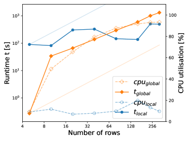
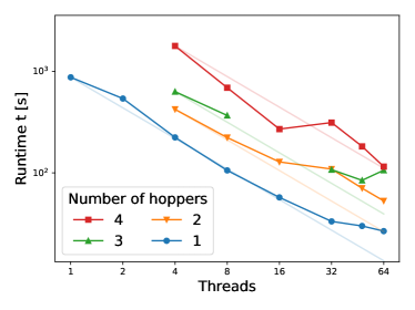
For both setups, the local time stepping struggles to keep pace with global time stepping unless the setups grow large. Strong and weak scalability are good.
Cluster topology, active clusters and concurrency level.
Both simulations kick off with around clusters. As the particles assemble within the hopper or pile up on the staircase, we obtain larger clusters. This is counteracted by small step sizes from complex interactions reducing the possible interaction range of any single particle in a given step. A global time stepping scheme hence suffers from the stiffness of individual particle interactions, whereas the local time stepping always manages to advance some clusters aggressively forward in time. Nevertheless, the permanent topology changes and rollbacks imply that the local time stepping’s overhead is very big. We have to simulate a significant number of particles to make the local time stepping overtake its global cousin (Figure 15).
The free fall ahead of any particle hitting the geometry, or a free fall once the particles leave the hopper resembles the behaviour in previous studies. These phases scale. The computationally expensive middle phase does not scale that well, and our scaling curves become non-smooth, reflecting the anarchic rearrangement of clusters. The algorithm’s concurrency changes permanently.
Time step size distribution.
The free fall prior to any particle hitting the obstacle allows the particles to advance at the same pace independent of local or global time stepping. As all particles start with a hard-coded initial downfall velocity (we omit gravity), we can predict a reasonable initial .
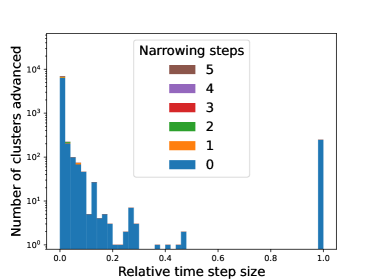
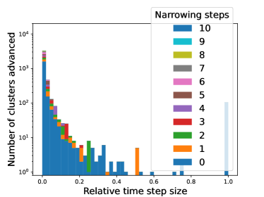
Once the particles hit the hopper or staircase, we get a more complicated time step size distribution (Figure 16): Clusters advance with different time step sizes, while notably the staircase enforces quite a lot of narrowing. We obtain huge clusters at time, where we have to try out smaller and smaller time step sizes, before the algorithm finds an effective time step size.
Contact points and particle interactions.
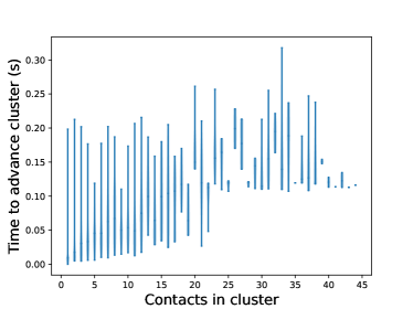
With complex particle geometries, the cost to solve the momentum exchange equations becomes unpredictable (Figure 17). The staircase, on average, produces fewer contacts per cluster, as the clusters are smaller. Yet, it becomes impossible to see a clear correlation between the number of contact points per cluster and the time required to solve the arising equation system. Due to a comparison with previous results, we can conclude that the complex geometric shapes have to cause this effect.
9 Conclusion
Local time stepping can be characterised in several ways: First, we have to decide between optimistic and conservative time stepping. Optimistic time stepping follows a trial-and-error approach. We start with a time step that is as large as possible, but, in the case of failure, i.e. penetration of physically incompressible objects, roll back, reduce the time step size and recompute until we have found an admissible step size. In conservative time stepping, we underestimate the admissible time step size all the time such that we can guarantees an admissible step size without any penetration. Second, local time stepping can be characterised through its granularity. Individual particles could progress with their own time step size, or we could cluster them and make the clusters advance in time with the same time step size. Global time stepping equals a degenerated cluster approach, where one cluster comprises all rigid bodies within the system. Finally, we have to differentiate local time stepping which allows arbitrary time step sizes from bucketing approaches, where sizes are picked from a finite set of discretised time slaps [8, 24]. The latter approach naturally leads into subcycling.
Our approach strives for a compromise between the extremes, constructing a bespoke, efficient variant: The clustering in combination with the narrowing yields a pessimistic approach, while the global scheme remains optimistic and hence requires rollbacks occasionally. We try to advance clusters hosting many particles in one rush, yet allow each particle to join another cluster in every single time step. At the same time, our flavour of local time stepping does not discretise time into fixed subintervals. As we consolidate particles of one cluster such that they start from the same time stamp and advance with the same time step size, we however constrain the progress in time such that particles do not advance totally anarchically.
Throughout the involved algorithmic subsets, we employ a multiscale language to speed the calculations up: Particles are represented by different shapes of increasing geometric complexity, we look at problems within a space-time setting, where we zoom into the time region of interest, and we employ various geometric representations to rule out potential overlaps of the particles’ -regions early. This way, we can harvest the efficiency promised by local time stepping—particles far away from potential collisions advance quickly [23].
While the efficiency gains obtained due to local time stepping are impressive, one major challenge is omitted: Load balancing local time stepping schemes is difficult. Without subcycling and any fixed cluster association, our algorithm yields algorithmic phases of varying concurrency all the time, and the load per compute step is difficult to predict. On a shared memory node, we rely on work stealing to level out imbalances. This works yet requires sufficient workload per step, which we do not obtain in all scenarios.
Two algorithmic degrees of freedom to address this issues are not further discussed in the present paper: DEM would allow us to mask out clusters artificially. In phases with many active clusters, it might be reasonable not to advance all algorithms, but to rule out some clusters which are then updated later when otherwise only few clusters are active. At the same time, it might be reasonable to abandon the synchronisation of the compute phases. We run through the six compute steps per time step one by one. Future implementation might want to try to overlap the individual steps.
Future work also will have to develop algorithms that scale beyond compute node boundaries. This could either be achieved through tasking approaches which allow for task migration beyond nodes. Alternatively, it might be reasonable to use larger clusters spanning multiple nodes. As highlighted, global time stepping is equivalent to working with one cluster only in our formalism. Excessively large clusters introduce a hybrid between local and global time stepping, and might be key to scale up local time stepping schemes over parallel machines.
References
- [1] Catch2. https://github.com/catchorg/Catch2/releases/tag/v3.1.1. Accessed: 2023-07-07.
- [2] E. Catto et al., Fast and simple physics using sequential impulses, in Proceedings of game developer conference, 2006.
- [3] P. A. Cundall and O. D. L. Strack, A discrete numerical model for granular assemblies, Géotechnique, 29 (1979), pp. 47–65, https://doi.org/10.1680/geot.1979.29.1.47, https://doi.org/10.1680/geot.1979.29.1.47, https://arxiv.org/abs/https://doi.org/10.1680/geot.1979.29.1.47.
- [4] Eigen. https://eigen.tuxfamily.org/index.php. Accessed: 2023-07-07.
- [5] Embree. https://github.com/embree/embree/releases/tag/v3.13.5. Accessed: 2023-07-07.
- [6] Z. Ferguson, M. Li, T. Schneider, F. Gil-Ureta, T. Langlois, C. Jiang, D. Zorin, D. M. Kaufman, and D. Panozzo, Intersection-free rigid body dynamics, ACM Transactions on Graphics (SIGGRAPH), 40 (2021).
- [7] GLFW. https://github.com/glfw/glfw/releases/tag/3.3.6. Accessed: 2023-07-07.
- [8] L. He, X. Ban, X. Liu, and X. Wang, Individual Time Stepping for SPH Fluids, in EG 2015 - Short Papers, B. Bickel and T. Ritschel, eds., The Eurographics Association, 2015, https://doi.org/10.2312:egsh.20151010.
- [9] K. Iglberger and U. Rüde, Massively parallel granular flow simulations with non-spherical particles, Computer Science - Research and Development, 25 (2010), pp. 105–113, https://doi.org/10.1007/s00450-010-0114-4.
- [10] T. R. Kane and D. A. Levinson, Dynamics, theory and applications, McGraw Hill, 1985.
- [11] K. Krestenitis, T. Weinzierl, and T. Koziara, Fast dem collision checks on multicore nodes., in Parallel processing and applied mathematics : 12th International conference, PPAM 2017, Lublin, Poland, September 10-13; revised selected papers. Part 1., R. Wyrzykowski, J. J. Dongarra, E. Deelman, and K. Karczewski, eds., no. 10777 in Lecture Notes in Computer Science, 2018, pp. 123–132.
- [12] H. Kruggel-Emden, S. Rickelt, S. Wirtz, and V. Scherer, A study on the validity of the multi-sphere discrete element method, Powder Technology, 188 (2008), pp. 153–165, https://doi.org/https://doi.org/10.1016/j.powtec.2008.04.037, https://www.sciencedirect.com/science/article/pii/S0032591008002143.
- [13] L. Lan, D. M. Kaufman, M. Li, C. Jiang, and Y. Yang, Affine body dynamics: Fast, stable and intersection-free simulation of stiff materials, ACM Trans. Graph., 41 (2022), https://doi.org/10.1145/3528223.3530064, https://doi.org/10.1145/3528223.3530064.
- [14] M. Li, D. M. Kaufman, and C. Jiang, Codimensional incremental potential contact, ACM Trans. Graph. (SIGGRAPH), 40 (2021).
- [15] T. Y. Li and J. S. Chen, Incremental 3D collision detection with hierarchical data structures, Proceedings of the ACM symposium on Virtual reality software and technology 1998 - VRST ’98, 1998 (1998), pp. 139–144, https://doi.org/10.1145/293701.293719.
- [16] libigl. https://github.com/libigl/libigl/releases/tag/v2.3.0. Accessed: 2023-07-07.
- [17] S. Luding, Introduction to discrete element methods, European Journal of Environmental and Civil Engineering, 12 (2008), pp. 785–826.
- [18] P. J. Noble and T. Weinzierl, A multiresolution discrete element method for triangulated objects with implicit time stepping, SIAM Journal on Scientific Computing, 44 (2022), pp. A2121–A2149, https://doi.org/10.1137/21M1421842, https://doi.org/10.1137/21M1421842, https://arxiv.org/abs/https://doi.org/10.1137/21M1421842.
- [19] A. D. Rakotonirina and A. Wachs, Grains3D, a flexible DEM approach for particles of arbitrary convex shape - Part II: Parallel implementation and scalable performance, Powder Technology, 324 (2018), pp. 18–35, https://doi.org/10.1016/j.powtec.2017.10.033, https://doi.org/10.1016/j.powtec.2017.10.033.
- [20] E. Rougier, A. Munjiza, and J.-P. Latham, Shape selection menu for grand scale discontinua systems, Engineering Computations, 21 (2004), pp. 343–359, https://doi.org/10.1108/02644400410519820.
- [21] A. Schmitt, J. Bender, and H. Prautzsch, On the convergence and correctness of impulse-based dynamic simulation, Technical Report 17, University of Karlsruhe, 2005.
- [22] SIMDe. https://github.com/simd-everywhere/simde/releases/tag/v0.7.2. Accessed: 2023-07-07.
- [23] H. Sitaraman and R. Grout, An adaptive timestepping methodology for particle advance in coupled cfd-dem simulations, (2018).
- [24] H. Sitaraman and R. Grout, An adaptive timestepping methodology for particle advance in coupled cfd-dem simulations, (2018).
- [25] TBB. https://www.oreilly.com/library/view/intel-threading-building/9780596514808/. Accessed: 2023-10-12.
- [26] TetGen. https://wias-berlin.de/software/index.jsp?id=TetGen&lang=1. Accessed: 2023-07-07.
- [27] The Computational Geometry Algorithms Library. https://www.cgal.org/2022/10/12/cgal551/. Accessed: 2023-07-07.
- [28] B. Wang, Z. Ferguson, T. Schneider, X. Jiang, M. Attene, and D. Panozzo, A large-scale benchmark and an inclusion-based algorithm for continuous collision detection, ACM Trans. Graph., 40 (2021), https://doi.org/10.1145/3460775, https://doi.org/10.1145/3460775.
- [29] T. Weinhart, L. Orefice, M. Post, M. P. van Schrojenstein Lantman, I. F. Denissen, D. R. Tunuguntla, J. Tsang, H. Cheng, M. Y. Shaheen, H. Shi, P. Rapino, E. Grannonio, N. Losacco, J. Barbosa, L. Jing, J. E. Alvarez Naranjo, S. Roy, W. K. den Otter, and A. R. Thornton, Fast, flexible particle simulations — an introduction to mercurydpm, Computer Physics Communications, 249 (2020), p. 107129, https://doi.org/https://doi.org/10.1016/j.cpc.2019.107129, https://www.sciencedirect.com/science/article/pii/S0010465519304357.