Microlensing Discovery and Characterization Efficiency in the Vera C. Rubin Legacy Survey of Space and Time

Abstract

The Vera C. Rubin Legacy Survey of Space and Time will discover thousands of microlensing events across the Milky Way Galaxy, allowing for the study of populations of exoplanets, stars, and compact objects. It will reach deeper limiting magnitudes over a wider area than any previous survey. We evaluate numerous survey strategies simulated in the Rubin Operation Simulations (OpSims) to assess the discovery and characterization efficiencies of microlensing events. We have implemented three metrics in the Rubin Metric Analysis Framework: a discovery metric and two characterization metrics, where one estimates how well the lightcurve is covered and the other quantifies how precisely event parameters can be determined. We also assess the characterizability of microlensing parallax, critical for detection of free-floating black hole lenses, in a representative bulge and disk field. We find that, given Rubin’s baseline cadence, the discovery and characterization efficiency will be higher for longer duration and larger parallax events. Microlensing discovery efficiency is dominated by observing footprint, where more time spent looking at regions of high stellar density including the Galactic bulge, Galactic plane, and Magellanic clouds, leads to higher discovery and characterization rates. However, if the observations are stretched over too wide an area, including low-priority areas of the Galactic plane with fewer stars and higher extinction, event characterization suffers by $>10\%$, which could impact exoplanet, binary star, and compact object events alike. We find that some rolling strategies (where Rubin focuses on a fraction of the sky in alternating years) in the Galactic bulge can lead to a 15-20% decrease in microlensing parallax characterization, so rolling strategies should be chosen carefully to minimize losses.

1 Introduction

Microlensing occurs when light coming from a distant star (source) is deflected by a foreground object (lens) located along the observer-source line of sight. As a result, multiple images of the source are formed, and since the images are usually unable to be resolved, the source appears to be photometrically magnified (Paczynski, 1986). Since the effect depends on the gravitational influence of the lens and not its luminosity, microlensing is a powerful tool to find and weigh dim objects like cool low-mass stars, planets (e.g. Gaudi, 2012), neutron star candidates, and stellar-mass black hole candidates (e.g. Lu et al., 2016; Lam et al., 2022; Sahu et al., 2022; Mróz et al., 2022; Lam & Lu, 2023) that are otherwise hard to observe.

The microlensing discovery rate increases with the stellar density; therefore, it is highest when observing crowded parts of the sky like the Galactic bulge, Galactic plane, and Large and Small Magellanic Clouds (LMC and SMC). Previous and ongoing dedicated microlensing surveys (e.g. OGLE (Udalski et al., 2015), MOA (Sumi et al., 2003), KMTNet (Kim et al., 2018), MACHO (Alcock et al., 2000), and EROS (Moniez et al., 2017)) have focused on these areas of high stellar density. All-sky surveys offer the opportunity to explore microlensing throughout the Galaxy. Observing throughout the Galaxy gives us the opportunity to probe Galactic structure (e.g. Moniez, 2010; Moniez et al., 2017) and constrain how the mass function of the lenses, such as black holes, changes throughout the galaxy. Observations of the Magellanic Clouds also offer an opportunity to explore compact halo objects and extragalactic stellar remnants, which can then be compared with those of the Milky Way Galaxy.

The Vera C. Rubin Observatory Legacy Survey of Space and Time (LSST) will survey 18,000 deg² including parts of the Galactic plane along with LMC and SMC as part of its Wide Fast Deep (WFD) survey. Surveying at least every 2-3 days is imperative to a high discovery rate of microlensing events (Street et al., 2018; Sajadian & Poleski, 2019). The Vera C. Rubin Observatory (Rubin) is going through a community-driven cadence optimization process described in detail in Bianco et al. (2022). A series of hundreds of cadence simulations called Operation Simulations (OpSims) were created to mock scheduled observations, using the Rubin scheduler (Naghib et al., 2019) with LSST simulations framework (Connolly et al., 2014). There are families of simulations which focus on optimizing particular qualities such as the region of sky covered in the WFD (or “footprint”), the frequency of observations (or “cadence”), filter balance, and rolling. A rolling cadence is when we divide the sky into multiple sections and in some years Rubin will observe some sections with an increased number of observations and in other years it will focus its observations to the other sections. These are evaluated using the Metric Analysis Framework (MAF, Jones et al., 2014) which contains both metrics from the Rubin project development team and contributed by the community for particular science cases.

In this work, we have written and tested a multi-faceted MicrolensingMetric (see Section 2.1) on the set of OpSims from v2.0 to v3.0 which investigates the detection and characterization of microlensing events. We have also tested the effect of changes to footprint and a rolling cadence on the characterization of microlensing events with a parallax signal outside the context of the MAF. The rest of the paper is organized as follows. In Section 1.1 we introduce standard microlensing terminology used throughout. In Section 2 we introduce the metric used to assess the microlensing yields, the sample of microlensing events assessed, and our methodology for determining microlensing parallax characterization. In Section 3 we explore the results of the MicrolensingMetric for relevant OpSims and parallax characterization for select OpSims. Finally, in Section 4 we discuss implications and summarize conclusions.

1.1 Microlensing Parameters

We will introduce the standard microlensing parameters that were used to model microlensing events (Paczynski, 1986). The characteristic length scale of a microlensing event is known as the angular Einstein radius, which is given by

$$\theta_{\rm E}=\sqrt{\frac{4GM}{c^{2}}\left(\frac{1}{D_{\rm L}}-\frac{1}{D_{\rm S}}\right)},$$ (1)

where $M$ is the lens mass, $D_{\rm L}$ is the distance to the lens from the observer, and $D_{\rm S}$ is the distance to the source from the observer. $\theta_{\rm E}$ and the relative proper motion of the source and lens ($\mu_{\rm rel}$) can be used to define the characteristic timescale, the Einstein crossing time:

$$t_{\rm E}=\frac{\theta_{\rm E}}{\mu_{\rm rel}}.$$ (2)

So events with more massive lenses tend to have longer $t_{\rm E}$. Neglecting the effects of parallax, the projected separation between the lens and source in units of Einstein radii as a function of time is the impact parameter:

$$u(t)=\sqrt{u_{0}^{2}+\left(\frac{t-t_{0}}{t_{\rm E}}\right)^{2}},$$ (3)

where $u_{0}$ is the closest projected separation and $t_{0}$ is the time of closest approach. Microlensing events are detected as a temporary photometric magnification. The amplification of a point source-point lens microlensing event is given by:

$$A(t)=\frac{u^{2}+2}{u\sqrt{u^{2}+4}}.$$ (4)

The amplification is maximized when $u=u_{0}$. We can use this signal in inferring the lens mass, but a measurement of the lens mass requires either a galactic model or additional observable constraints on $D_{L}$, $D_{S}$, and $\mu_{\rm rel}$. When the lens is luminous or there are neighboring stars, the light from the source may be blended with them. This is characterized by the source flux ($F_{\rm S}$) and the blend flux:

$$F_{\rm B}=F_{\rm L}+F_{\rm N},$$ (5)

where $F_{\rm L}$ is the lens flux and $F_{\rm N}$ is the neighbor flux. So the flux as a function of time is then:

$$F(t)=F_{\rm S}A(t)+F_{\rm B}.$$ (6)

The blend source flux fraction or blend fraction is $b_{\rm sff}=F_{\rm S}/(F_{\rm B}+F_{\rm S})$.

The motion of the Earth around the Sun introduces a higher order effect in microlensing events known as the microlensing parallax (Gould, 1992), $\bm{\pi_{\rm E}}$, the magnitude of which is defined as

$$\pi_{\rm E}=\frac{\pi_{\rm LS}}{\theta_{\rm E}},$$ (7)

where $\pi_{\rm LS}$ is the relative lens-source parallax ($\pi_{\rm LS}=(1\textrm{AU})(\frac{1}{D_{\rm L}}-\frac{1}{D_{\rm S}})$ ). The signal strength depends predominantly on the difference between the lens parallax and the source parallax but also on the time of the year. In effect, the changing position of an observer following the Earth’s orbit changes the optical axis of the lensing configuration. Microlensing events much shorter than a year tend to exhibit a negligible parallax signal. By convention, $\bm{\pi_{\rm E}}$ is a vector that can be broken down into East and North components, $\bm{\pi_{\rm E}}=[\pi_{E,E},\pi_{E,N}]$, pointed in the direction of $\mu_{\rm rel}$, the relative lens-source proper motion. Along with $\mu_{\rm rel}$, which can be constrained by the galactic model, and $t_{\rm E}$, $\pi_{\rm E}$ can be used to determine the mass of the lens:

$$M=\frac{\mu_{\rm rel}t_{\rm E}}{\kappa\pi_{\rm E}}$$ (8)

where $\kappa\equiv\frac{4G}{(\textrm{1 AU})c^{2}}\approx 8.144~{}\mathrm{mas}/M_{\odot}$.

For a physical understanding of where microlensing events lie in the $\pi_{\rm E}-t_{\rm E}$ plane see Figure 1. Here we plot simulated events from Population Synthesis for Compact-object Lensing Events (PopSyCLE, Lam et al., 2020). Events with less massive, often stellar, lenses tend to have shorter $t_{\rm E}$ and larger $\pi_{\rm E}$; whereas, events with more massive, often compact object, lenses tend to have longer $t_{\rm E}$ and smaller $\pi_{\rm E}$.

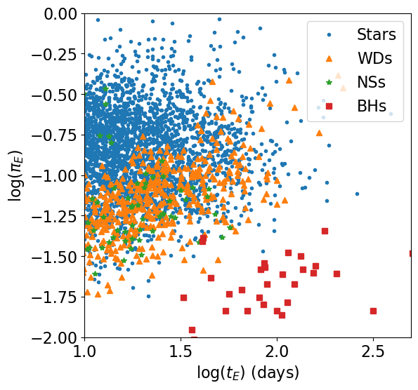
Figure 1: Microlensing parallax (Eq. 7) vs Einstein crossing time (Eq. 2) for microlensing events simulated using PopSyCLE (Lam et al., 2020). Blue circles are stars, orange triangles are white dwarfs, green stars are neutron stars, and red squares are black holes. The ranges of $t_{\rm E}$ and $\pi_{\rm E}$ are cropped to match Figures 8-12. More massive lenses tend to be towards the bottom right of this plot.

2 Methodology

In this section we describe a suite of metrics which are used to assess how the relative number of detected and characterized microlensing events is affected by the survey strategy. This is not expected to produce a realistic yield for Rubin LSST. Instead, it is expected to inform which strategies are beneficial for microlensing and do not make the microlensing science case inviable, even if they negatively affect the microlensing yield. There are three metrics within the MAF framework which are simulated without microlensing parallax and one metric outside the MAF framework simulated with microlensing parallax (see Table 1). The results for the three metrics in the MicrolensingMetric are described in Sections 3.1-3.15 and the parallax characterization metric results are in Section 3.16.

Metric	Simulated Sample	Metric Description
MicrolensingMetric - Discovery Metric	$t_{\rm E}$-only (Section 2.2)	2 points with $\geq 3\sigma$ difference
MicrolensingMetric - Npts Metric	$t_{\rm E}$-only (Section 2.2)	10 points within $t_{\rm 0}\pm t_{\rm E}$
MicrolensingMetric - Fisher Metric	$t_{\rm E}$-only (Section 2.2)	Analytic Fisher with $\frac{\sigma_{t_{\rm E}}}{t_{\rm E}}<0.1$
Parallax Characterization Metric	$t_{\rm E}+\pi_{\rm E}$ (Section 2.3)	Numerical Fisher with $\pi_{\rm E}>2\sigma_{\pi_{\rm E}}$ & $t_{\rm E}>2\sigma_{t_{\rm E}}$

Table 1: Description, name, and input sample of metrics used to analyze microlensing efficiency. The Sample column refers to the sample of microlensing events that were evaluated with the metric. The three metrics in the MicrolensingMetric are not simulated with parallax and are all-sky. The parallax characterization metric used a sample with parallax for two small patches of the sky.

2.1 MicrolensingMetric

The MicrolensingMetric is integrated with the rubin_sim package and provides a set of metrics for evaluating the efficacy of cadences in detecting, alerting, and characterizing microlensing events. The metric relies on a simulated population of microlensing events described in detail in Section 2.2. We can calculate the discovery efficiency by finding the fraction of events with at least 2 points on the rise of the lightcurve with at least a $3\sigma$ difference between the highest and lowest magnitude points. We can also specify a number of days before the peak time that the event must be “triggered” by, since ensuring the observation of the peak in follow-up is important for lightcurve characterization. (Note that while this functionality is in the metric and is important for event follow-up, including exoplanet and black hole candidates, an exploration of alerting efficiency is beyond the scope of this paper). There are also two metrics for the characterization of the lightcurves purely from Rubin observations. There is a basic metric that quantifies the number of points (Npts) within $t_{\rm 0}\pm t_{\rm E}$ which estimates the coverage of the lightcurve. Npts Metric was used as a proxy for characterization and figure of merit is the fraction of events with at least 10 points within $t_{\rm 0}\pm t_{\rm E}$. There is also a metric that calculates the Fisher matrix for each event and returns the fractional uncertainty in $t_{\rm E}$ (see Section 2.1.1). See Figure 2 for a summary of the MicrolensingMetric functionality.

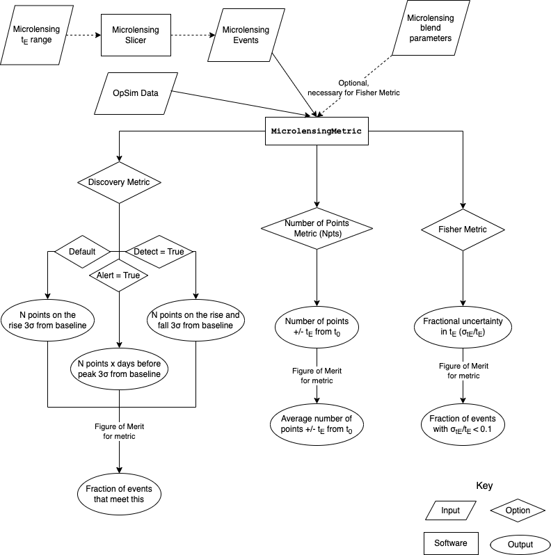
Figure 2: Flowchart of the MicrolensingMetric functionality. The user can either input a $t_{\rm E}$ range and generate microlensing events with a function known as a “Slicer”, or the user can input the events. The user can then choose to use the Discovery Metric, Npts Metric, or Fisher Metric. The Discovery Metric, by default, finds the fraction of events with N points on the rising side with at least a 3$\sigma$ difference from baseline. The user can select detect=True to find at least N points on both the rising and falling side or alert=True to require the N points on the rising side to be a certain number of days before the peak. Npts Metric returns the number of points within $t_{\rm 0}\pm t_{\rm E}$ and Fisher Metric returns the fraction of events with a fractional $t_{\rm E}$ uncertainty $<0.1$.

2.1.1 Fisher Matrix

To characterize events, we want to ensure an adequate photometric cadence during the information-bearing part of the lightcurve. This is essential for determining microlensing parameters such as $t_{\rm E}$ which allow us to infer physical properties of the lens and source populations. We adapt the Fisher matrix approach, which is widely used in many fields such as cosmology (e.g. Jungman et al., 1996; Albrecht et al., 2006). To quantify how precisely parameters can be recovered, we use a fiducial model, namely that our simulated parameters correspond to the actual parameter estimates. According to the Cramer-Rao inequality, the Fisher matrix allows us to calculate a lower bound on the uncertainty.

In the MAF, since we have simulated the microlensing event population, we can use their known parameters to evaluate the Fisher matrix

$$I_{i,j}=\sum_{k=1}^{N_{\rm{data}}}\frac{1}{\sigma^{2}_{F}(t_{k})}\left(\frac{\partial F_{\mathrm{model}}(t_{k})}{\partial p_{i}}\right)\left(\frac{\partial F_{\mathrm{model}}(t_{k})}{\partial p_{j}}\right)$$ (9)

where $p_{i}$ and $p_{j}$ denote the event parameters: $t_{\rm E},t_{0},u_{0}$, and the blend and baseline flux parameters for each passband; $t_{k}$ is each time of observation; $N_{\rm data}$ is the length of the entire dataset (including all passbands); $F$ is the flux; and $\sigma_{F}$ is the error in the flux. Assuming Gaussian errors on each observable, the Fisher information matrix is approximately the inverse of the covariance matrix. One element of this matrix will be the uncertainty in $t_{\rm E}$, so we can calculate the fractional uncertainty $\sigma_{t_{\rm E}}/t_{\rm E}$. We treat an event as well characterized if $\sigma_{t_{\rm E}}/t_{\rm E}<10\%$. This threshold indicates if we can constrain the lens mass or if its error budget is dominated by the unknown $t_{\rm{E}}$. An advantage of using a Fisher information matrix is that it can account for the contribution of both the lightcurve coverage and the uncertainty of the observations, $\sigma^{2}_{F}(t_{k})$, to the uncertainties of the model parameters.

We can evaluate the Fisher matrix by taking analytic derivatives with respect to each of the parameters ($t_{\rm E}$, $t_{0}$, $u_{0}$, $F_{\rm S}$, and $F_{\rm B}$) using SymPy (Meurer et al., 2017). Speeding up the calculation of the MicrolensingMetric is key for evaluating many OpSims, and Eq. 9 is the best suited approximation since it only relies on first derivatives. To optimize the evaluation of the analytic Fisher metric, we use the common subexpression elimination part of SymPy jointly finding suitable substitutions for the parameters.

2.2 Sample of Microlensing Events

In order to cover the phase space of microlensing events in a heuristic way, we simulate across the whole sky in HEALPIX and weight the probability of having a microlensing event at a particular RA and Dec with the number of stars squared in the TRILEGAL stellar map simulated for LSST (Dal Tio et al., 2022). The number of events should scale with the square of the visible density which traces the square of all compact objects.

For each metric, we split the population into $t_{\rm E}$ bins and generated 10,000 events for each $t_{\rm E}$ bin. The events were simulated with uniform distributions of $t_{\rm E}$ from minimum to maximum $t_{\rm E}$ in the bin and $t_{0}$ from the minimum to maximum observation date in the given OpSim. For the discovery metric we make 9 $t_{\rm E}$ bins: 1-5 days, 5-10 days, 10-20 days, 20-30 days, 30-60 days, 100-200 days, 200-500 days, and 500-1000 days. For the Npts and Fisher metrics we analyze a subset of these bins for computational efficiency (10- 20 days, 20-30 days, 30-60 days, and 200-500 days). We break the events up into $t_{\rm E}$ bins so that we can analyze different populations of objects separately. Since $t_{\rm E}\propto\frac{\sqrt{M_{\rm lens}}}{\mu_{\rm rel}\sqrt{\pi_{\rm LS}}}$, various $t_{\rm E}$ are use related to different populations of objects, from low mass stars and free floating planets with short $t_{\rm E}$, to black holes with long $t_{\rm E}$. We find that longer $t_{\rm E}$ events are more likely to be observed over the course of their duration than shorter $t_{\rm E}$ events (see Figure 4), and a rolling cadence (which is where Rubin focuses on a fraction of the sky in alternating years) could leave large parts of long $t_{\rm E}$ events unobserved (see Section 3.14). So if we evaluated events with $1<t_{E}<1000\,{\rm d}$ together, then we would not see the strength of the effect of changing the cadence. The events were also simulated with uniform distribution of $u_{0}$ from 0 to 1. While Rubin will likely detect events with lower magnifications than this, as OGLE and other surveys do, this is an approximation to compare between OpSims.

To simulate a typical star as the source of our microlensing events, we found the mean stellar magnitude in each filter of the TRILEGAL map and used that as the source magnitude for all the events. These values are: $u$: 25.2, $g$: 25.0, $r$: 24.5, $i$: 23.4, $z$: 22.8, $y$: 22.5. Note these are close to the detection limit of Rubin.

For the Fisher matrix calculation (see Section 2.1.1), it is important to take blending into account. A high blend fraction can decrease the certainty of parameters, since for blended events the apparent baseline becomes brighter and the blend fraction, $t_{\rm E}$, and $u_{0}$ are degenerate. We estimated that in the locations of high stellar density where most of these events occur that the blend fraction is $\sim 50\%$ or the flux from neighboring stars + the lens ($F_{\rm B}$) is approximately equal to the source flux ($F_{\rm S}$) (see Figure 3 of Tsapras et al., 2016).

2.3 Parallax characterization

The methods for evaluating the effect of the cadence on microlensing in Section 2.1 did not include the parallax effect. Characterizing the microlensing parallax is important for inferring the mass and nature of the lenses (see Eq. 8; see Figure 13 of Lam et al. (2020)). Hence, on a subset of OpSims we simulated 100,000 events in a representative bulge and disk field including parallax to determine how the characterization of lightcurves including parallax are affected by cadence. We are particularly interested in how rolling affects the characterization of microlensing parallax, as this is a periodic effect in long enough events.

We determined how well we could characterize each event by taking numerical derivatives of each of the parameters ($t_{0},t_{\rm E},u_{0},\pi_{E,E},\pi_{E,N}$, blend parameter, and source magnitude) and applied Eq. 9 to determine the Fisher information matrix. Numerical derivatives were computed by simulating models where the parameters differed by a tolerance of (0.01 $\times$ value of the parameter) and the slope was calculated. The errors on the magnitude of each observation were determined using the calc_mag_error_m5() in rubin_sim. The lightcurves were modeled using Bayesian Analysis of Gravitational Lensing Events (BAGLE), an open-source microlensing event modeling and fitting code.

We simulated two patches of 100,000 events, one at RA = 263.89^∘, Dec = -27.16^∘, and the other at RA = 288.34^∘, Dec = 9.66^∘. The first is a representative bulge field and the second is a representative disk field in one of the pencil beam fields described in Street et al. (2023a). We used the observations in a square field of view 3.5^∘ across to mimic a Rubin field of view. The events were simulated with uniform distributions of $u_{0}$ from -1 to 1, log($t_{\rm E}$) from 5 to 600 days, $t_{0}$ from the minimum to maximum observation date in the given OpSim, $\pi_{\rm E}$ from 0 to 1, and $\phi$ from 0 to $2\pi$. Where $\phi$ determines the direction of the parallax by

$$\pi_{\rm E,N} = \pi_{\rm E}\sin(\phi)$$ (10)

$$\pi_{\rm E,E} = \pi_{\rm E}\cos(\phi).$$ (11)

Figure 3: Example plot of a characterizable event with $t_{\rm E}=161$ days and $\pi_{\rm E}=0.21$. Details of the simulation are described in Section 2.3. The parallax is characterized with a relative uncertainty of $\sigma_{\pi_{\rm E}}/\pi_{\rm E}=0.06$ and the Einstein time is characterized with $\sigma_{t_{\rm E}}/t_{\rm E}=0.06$. As is standard for achromatic microlensing events, all lightcurves are aligned and rescaled to the best data set. In this case, the r band serves as reference baseline.

The criteria for characterization of a lightcurve is for both $t_{\rm E}>2\sigma_{t_{\rm E}}$ and $\pi_{\rm E}>2\sigma_{\pi_{\rm E}}$. An example characterized event can be seen in Figure 3. These results are outside the context of the MicrolensingMetric and explored in Section 3.16.

3 Results

The Rubin OpSim team ran the MicrolensingMetric on 360+ OpSims. These OpSims have “families” which test for a particular aspect of the cadence such as filter distribution or Galactic plane footprint. We will describe the results of the MicrolensingMetric for each of the families of OpSims. See Table 2 for descriptions of the OpSims discussed here with descriptions of their relevance to microlensing and Galactic science. In this simulation, the Discovery Metric, Npts Metric, and Fisher Metric were all run. The Discovery Metric was configured such that 2 points $3\sigma$ above baseline were required on the rising side of the lightcurve. When we refer to the discovery efficiency, this refers to the fraction of simulated events that meet the Discovery Metric criteria, and when we refer to characterization efficiency, this refers to the fraction of simulated events that meet the Npts or Fisher Metric criteria. The retro baseline is described in detail in Jones et al. (2020) and the v2.0-v3.0 are described in detail in a Rubin technical note PSTN-055 (where baseline_v3.0_10yrs is the same as draft2_rw0.9_uz_v2.99_10yrs).

In general, the larger the footprint dedicated to the Galactic bulge and plane, the more microlensing events we can see and characterize. There is also a trend where longer duration microlensing events are less affected by observing strategy since they last long enough that most strategies eventually accumulate enough observations. Though, the exact cadence of observations is still important, especially for characterization of $t_{\rm E}$ and $\pi_{\rm E}$. We quantify how well the metrics perform by comparing their performance to the baseline_v2.0_10yrs OpSim. The results of the sample without parallax analyzed by the MicrolensingMetric are in Sections 3.1-3.15, and the parallax characterization metric results are in Section 3.16.

3.1 Baseline Family

Most estimates of the number of microlensing events Rubin is expected to discover are based on the baseline_2018a OpSim (i.e. Sajadian & Poleski, 2019). We can compare baseline_2018a to retro_baseline_v2.0_10yrs which uses a similar observation strategy to baseline_2018a, but implemented with updated software and updated throughput and weather inputs. Using retro_baseline_v2.0_10yrs as a comparison point to baseline_2018a means that we can compare the previous footprint and general observation strategy with newer simulations and evolving survey strategy options. More recent versions of the baseline (v2.0 and higher) of the OpSims leads to a $\gtrsim 50\%$ improvement in both discovery and characterization over the “retro” baseline due to the inclusion of the Galactic bulge and parts of the Galactic plane. baseline_retrofoot_v2.0_10yrs adopts the old footprint, but uses the v2.0 baseline strategy; whereas retro_baseline_v2.0_10yrs is a version of the retro footprint and strategy. See Figure 4 for a comparison of the baseline OpSims. The v2.0 performs slightly better than v2.1, since v2.1 includes the Virgo cluster which is not a traditional microlensing target and takes time away from other areas. v2.2 included optimizations to the code and a change in Deep Drilling Field (DDF) strategy which should not significantly affect microlensing. baseline_v3.0_10yrs spends less time on the galactic bulge and spreads out observations across the plane (see Street et al., 2023a, for detailed discussion). Covering this larger area leads to $\sim 10-20\%$ fewer events being characterized (Fisher and Npts metric), but $\sim 5-10\%$ more being discovered (Discovery metric), since there are fewer events in the galactic plane than the bulge due to the decrease in stellar density. A strategy similar to this could allow Rubin to better probe galactic structure, but may require increased follow-up to characterize the discovered microlensing events.

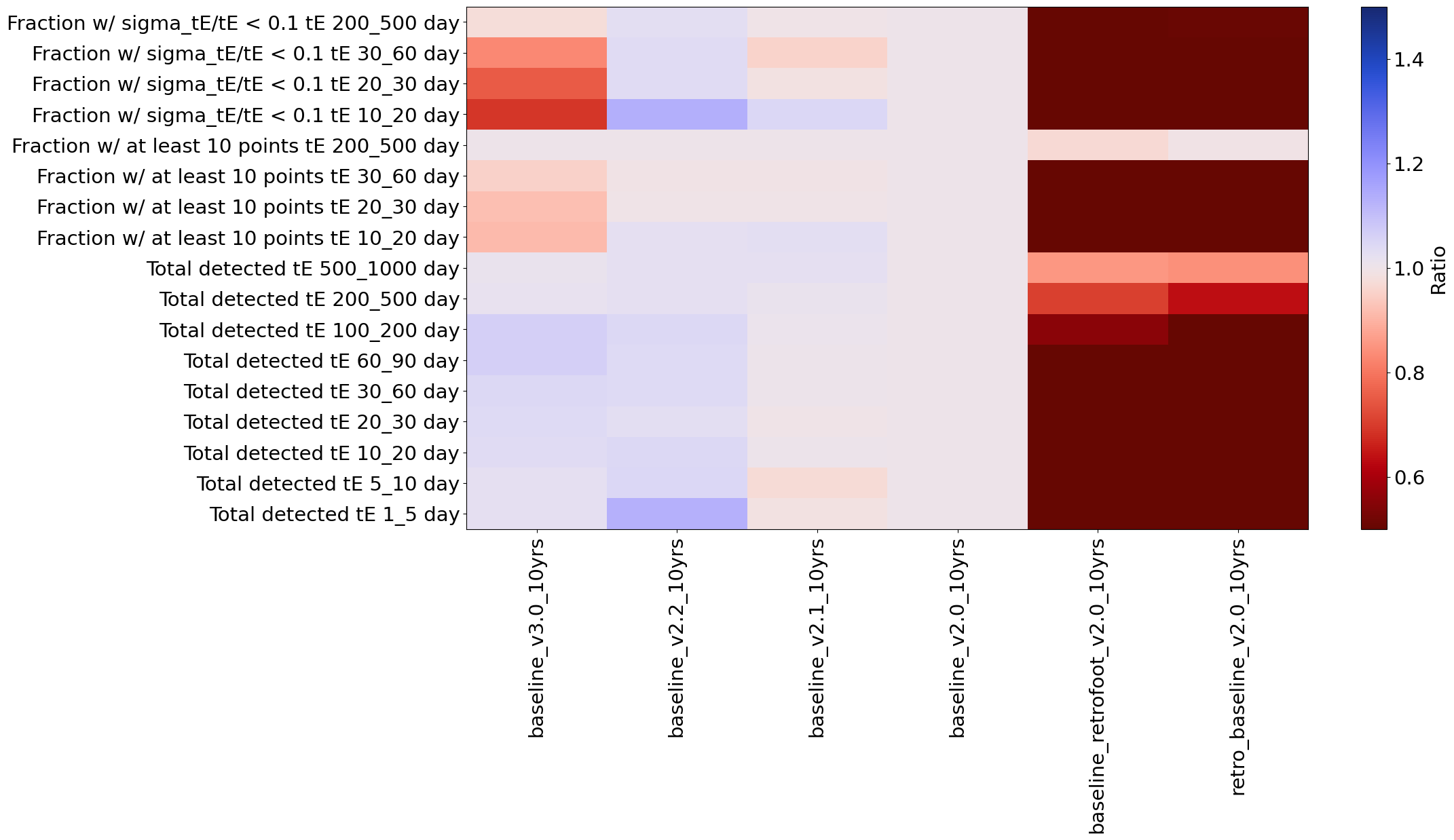
Figure 4: Comparison between MicrolensingMetric results for several distinct iterations of the Rubin baseline strategy. The colors show the fractional improvement relative to baseline_v2.0_10yrs, where blue means the metric has performed better relative to the baseline metric and red means it has performed worse. On the x-axis are each of the OpSims, where 10yrs means it was simulated for a 10 year LSST survey. On the y-axis are each of the metrics for a $t_{\rm E}$ range compared to their values for baseline_v2.0_10yrs. Shorter events (smaller $t_{\rm E}$) correspond with less massive objects such as brown dwarfs and low-mass stars, whereas longer events (larger $t_{\rm E}$) correspond to black holes. “Fraction w/ sigma_tE/tE $<$ 0.1” refers to the Fisher Metric; “Fraction w/ at least 10 points” refers to the Npts Metric, and “Total detected” refers to the Discovery Metric. For example, “Fraction w/ sigma_tE/tE $<$ 0.1 tE 30_60 day” refers to the fraction of the 10,000 events with $30~{}\mathrm{days}\leq t_{\rm E}\leq 60~{}\mathrm{days}$ simulated as described in Section 2.2 with $\frac{\sigma_{t_{\rm E}}}{t_{\rm E}}<0.1$ as calculated by the Fisher Information Matrix. All of the current baselines show a $\gtrsim$ 50% improvement over the retro baseline.

3.2 Filter distribution (bluer_ and long_u families)

The bluer_ and long_u families explore the distribution of exposures in different filters. The bluer_ and long_u families have $\leq 15\%$ fewer characterized events than baseline_v2.0_10yrs (see Figure 14). This is likely true because we simulated the source magnitude using the mean magnitude of stars in each filter of the TRILEGAL map. The mean magnitude in the blue band is fainter, so the events are harder to detect with a higher fraction of bluer points. Having more points in bluer bands will also make the events harder to follow up. However, since there is currently a fixed baseline magnitude, further investigation must be done to find the optimal filter balance.

3.3 Presto Color and third visits in a night (presto_gapXX, presto_gapXX_mix, presto_half families, and long_gaps family)

This set of families explore “triplets” of observations described in detail in Bianco et al. (2019). This means there will be a third visit on the same night, some fraction of nights, (in the case of the presto families, see Figure 5) or a third visit the next night (in the case of the long_gaps family). Microlensing events decrease in discovery and characterization by 10-30% in the presto color family. In general, microlensing events do not change sufficiently in a single night to warrant a third visit that night, and taking time away from looking at more varied points in time greatly decreases the efficacy of microlensing detection and characterization. In some strategies, there is an improvement in discovery to events with $t_{\rm E}$ 1-10 days, which do change at this timescale, but at the large expense of the majority of events ($t_{\rm E}>10$ days) and to their characterization. There could also be an improvement to events with short-duration features such as microlensing events with a binary lens, though events with such features are a small fraction of events.

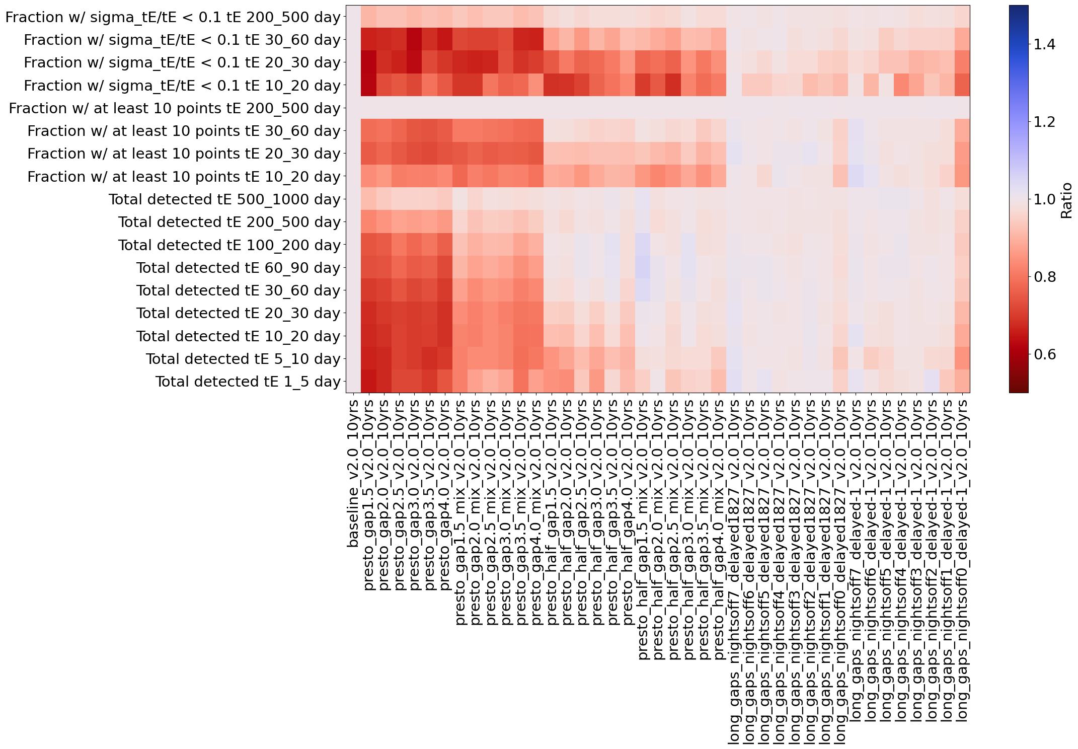
Figure 5: Same as Figure 4 but for the presto family which explores triplets of observations within one night. Since most microlensing events do not vary significantly over the course of a night, when observations are taken over a less varied time period, this decreases detection and characterization efficiency.

3.4 Twilight NEO v2.0 simulations (twilight_neo_nightpatternXX family)

The Twilight NEO family explores adding a twilight observing strategy, primarily looking for Near-Earth Objects. The SNR of observations is reduced, so the events, especially the short stellar events, suffer in characterizations by 5-10%. Some of the long events technically have more observations that overcome the SNR downsides, but the quality loss and systematic effects would make an analysis challenging despite the technically better relative assessment. This is a surprising result since we did not think the twilight observations would lead to a poorer coverage of the night-time events. A representative 3 of the 84 twilight_neo runs are plotted in Figure 15.

3.5 NES coverage as percentage of WFD coverage (vary_NES family)

These OpSims vary the coverage of the North Ecliptic Spur (NES) as a percentage of the WFD survey. The more the survey strategy covers the NES, the less we are able to cover the Galactic Bulge and Plane which causes the microlensing metric to suffer. For an NES coverage of 60-75%, there is a significant drop of about 15% in fraction of microlensing events that can be characterized (see Figure 14).

3.6 Galactic Plane coverage as a percentage of WFD coverage (vary_gp family)

These OpSims vary the visits to fields in the Galactic Plane as a percentage of the WFD survey from 1-100%. We see a significant decrease of microlensing characterization in strategies with gpfrac $\geq 0.55$. We see similarly to the NES OpSim family that technically if we cover the Galactic Plane more, that we characterize fewer microlensing events overall, since many of the microlensing events are concentrated towards the Galactic bulge (see Figure 6). However, it is scientifically interesting to be able to probe microlensing events throughout the Galactic plane.

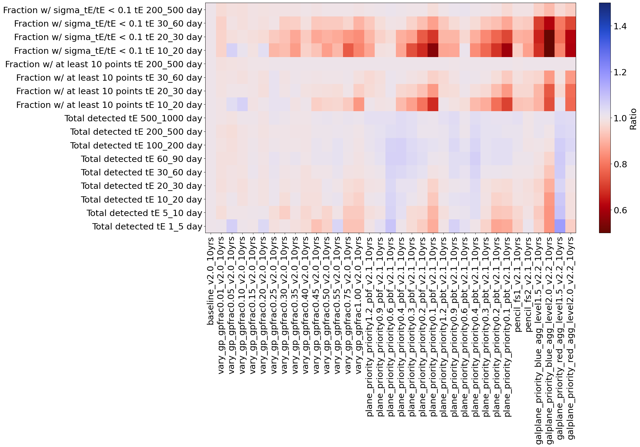
Figure 6: Same as Figure 4 but for the vary_gp, plane_priority, pencil, and galplane_priority, families. Covering regions of lower stellar density and/or high extinction (areas of priority less than 0.4 as defined in Street et al. (2023a)) leads to significant decrease in microlensing characterization efficiency. The pbf strategies do not include pencil beams selected in Street et al. (2023a) of scientific interest; whereas, the pbt strategies include them. While the number of detected and characterized microlensing events does not significantly differ between them, since the pencil beams were specifically chosen to optimize our ability to probe the Galaxy, the strategy is preferable. The size of the pencil beams does not appear to significantly affect microlensing efficiency.

3.7 Galactic Plane Footprint without pencil beams (plane_priority_priorityX.X_pbf_)

Using a map of the Galactic plane with scientifically motivated priorities assigned to each region (Street et al., 2023a) ranging between 0.1-1.2. Generally regions of lower stellar density and/or high extinction correspond to lower priority regions. These OpSims add regions of progressively less priority to the WFD footprint, so plane_priority_priority0.4 includes regions assigned priority $\geq 0.4$. These footprints do not include designated pencil beam fields selected for their scientific interest (see Section 3.8). We find that there is a drop in characterization efficiency for the long duration events in the plane priority map when it covers regions of priority of  0.4 or lower (see Figure 6), as a finite number of visits are distributed over too large a spacing in time for characterization. This matches what is found by the general Galactic plane metrics (Street et al., 2023a).

3.8 Galactic Plane Footprint with pencil beams (plane_priority_priorityX.X_pbt_)

These OpSims are the same as the plane priority without pencil beams (Section 3.7), except that pencil beam fields described in Street et al. (2023a) are added. We technically find similar results to the OpSims without pencil beams since we detect and characterize a similar number of events (see Figure 6). However, the pencil beam fields were picked specifically to optimize our ability to probe Galactic structure (along with other goals) throughout the Plane. Decades of microlensing surveys have looked at the Galactic bulge, but Rubin will enable us to look much deeper across the Galactic plane, so looking in strategic spots is helpful.

3.9 Pencil beam sizes (pencil_)

These OpSims vary the size of the pencil beam fields. As can be seen in Figure 6, the size of the pencil beams does not appear to affect the microlensing results.

3.10 Galactic Plane v2.2 Footprint and Filter Balance (galplane_priority_)

These OpSims explore what regions of the Galactic bulge and plane should be surveyed with a high number of visits determined by areas of scientific interest. level1.5 refers to a wider area surveyed with less intensity and level2.0 refers to a narrower area surveyed with more intensity (see Street et al., 2023a, for more details). There were also two filter balances tested: a “blue” one which allocates more exposures to u and g-bands and a “red” one which allocates more exposures to r, i, z, and y-bands. In all cases, level1.5 does better than level2, but in all cases baseline_v2.0_10yrs is better by $\sim 20-50\%$ (depending on strategy) at characterization. As explored in Section 3.6, as more of the Galactic plane is covered, we are able to characterize fewer events. Though, there is a peak in the discovery frequency.

The red strategy does better than blue (see Figure 6) since we had assumed a fixed baseline magnitude for all events with a brighter y and z band baseline (see Section 2.2). Hence, when the strategy is weighted towards y and z-bands, the metrics do better, but until a more complete simulation with a distribution of baseline magnitudes is carried out, this is not a significant result.

3.11 Good seeing (good_seeing_)

These OpSims add the requirement of at least 3 good seeing images per year per pointing. As the good seeing metric is prioritized, detection and characterization metrics worsen on the 10% level for characterization since it appears as though the footprint decreases and we end up with fewer events (see Figure 15). However, better template images for DIA could improve alerts and photometric accuracy but there is insufficient data to assess a suitable trade-off.

3.12 DDF Observing Strategies (ddf_)

Since the DDFs do not cover the Galactic plane, the more they have visits dedicated to them the fewer visits are available for regions in the Galactic plane. At the current level of the DDFs in the OpSims, it decreases short event characterization at the 10-15% level, but besides that it does not appear to significantly affect the microlensing science case.

3.13 Microsurveys

Microsurveys are “micro” observing surveys that take up to a few percent of the LSST observing time (explored in detail in a Rubin technical note PSTN-053). The two microsurveys of relevance for microlensing are roman_v2.0_10yrs and smc_movie_v2.0_10yrs. Since the rest of the surveys do not focus on microlensing targets, they only negatively impact microlensing on the 5-10% level since it takes time away from microlensing targets. See Figure 14 for a summary.

The roman_v2.0_10yrs microsurvey is designed to look at the footprint of the Nancy Grace Roman Galactic Bulge Time Domain Survey (GBTDS, Spergel et al., 2015). Observing the Roman field both during Roman’s $\sim 60-72$ day survey “seasons” and also filling in the multi-month gaps between its observations would be impactful. During Roman’s observing windows, concentrating more of the Galactic bulge observations on the Roman field could allow for simultaneous observations which could be used to calculate satellite parallax which can be used to constrain the mass of the lens (Yee et al., 2014). The number of increased visits to the Roman field should not be at a level that visits to the rest of the Galactic bulge are significantly reduced, but perhaps $\sim 0.5$ rolling since that did not seem to significantly negatively impact detection and characterization of events $>30$ days (see Section 3.14). The nominal GBTDS is planned to have seasons of $60-72$ days with multiple months-long gaps. While, some of these gaps are at times where Rubin cannot observe the Galactic bulge, there are some where Rubin could fill in Roman gaps. Filling in the photometry is particularly beneficial for characterizing long duration events that span multiple Roman seasons (Lam et al., 2023). The impact of a lack of space based astrometry during those times, though, is still to be determined. Work is in progress to further quantify the synergy between Roman and Rubin; see Street et al. (2023b) for more details.

The smc_movie_v2.0_10yrs includes two nights of high intensity observations of the SMC. Though the smc_movie_v2.0_10yrs survey decreases the characterization fraction of short duration events by 5-10%, the SMC is a target of scientific interest for microlensing for compact halo objects and to probe galactic structure in a nearby dwarf galaxy.

3.14 Rolling Cadence (rolling, roll_, _six_rolling)

In OpSims with a rolling cadence, the sky is broken up into 4-6 strips and observations are focused on half of the strips, alternating between years. There is already rolling incorporated in the baseline, though these OpSims explore different configurations of strips and if we should have a rolling cadence in the Galactic bulge. As can be seen in Figures 14 and 15, the rolling cadence generally does increase discovery of short events ($<10$ days) by $\sim 5\%$, especially rolling bulge OpSims. However, events with $t_{\rm E}>10$ days have a decrease in detection and characterization. In strategies in which the Galactic bulge and plane are explicitly included in rolled areas, detection efficiency decreases by 5-15% and characterization efficiency decreases by 10-40%. Most microlensing events have $t_{\rm E}>10$ days and it was expected that Rubin would alert on shorter duration events, not that it would be able to completely characterize them. Beyond explicitly rolling the Galactic bulge and plane, even if a region is not explicitly part of the rolling cadence, due to slew times and survey efficiency, those regions may also be affected. There is a decrease in characterization efficiency by 10-20% in six_rolling_ns2_rw0.9_v2.0_10yrs (see Figure 14) even though no region with significant microlensing population is part of the rolling footprint. Note that we have not included microlensing parallax here, see Section 3.16.

3.15 Varying exposure time (vary_expt and shave_)

This family varies the exposure times between 20 and 40 seconds and varies the individual depth (the shave_ runs). In general the shave series shows that longer exposure times are more effective for detecting microlensing events on the 10-15% level (see Figure 15). This makes sense since as the SNR increases, we can more effectively characterize the events. Note that this metric does not take into account variable blending. So longer exposures may lead to more blending which would lead to worse microlensing characterization.

3.16 Parallax Characterization

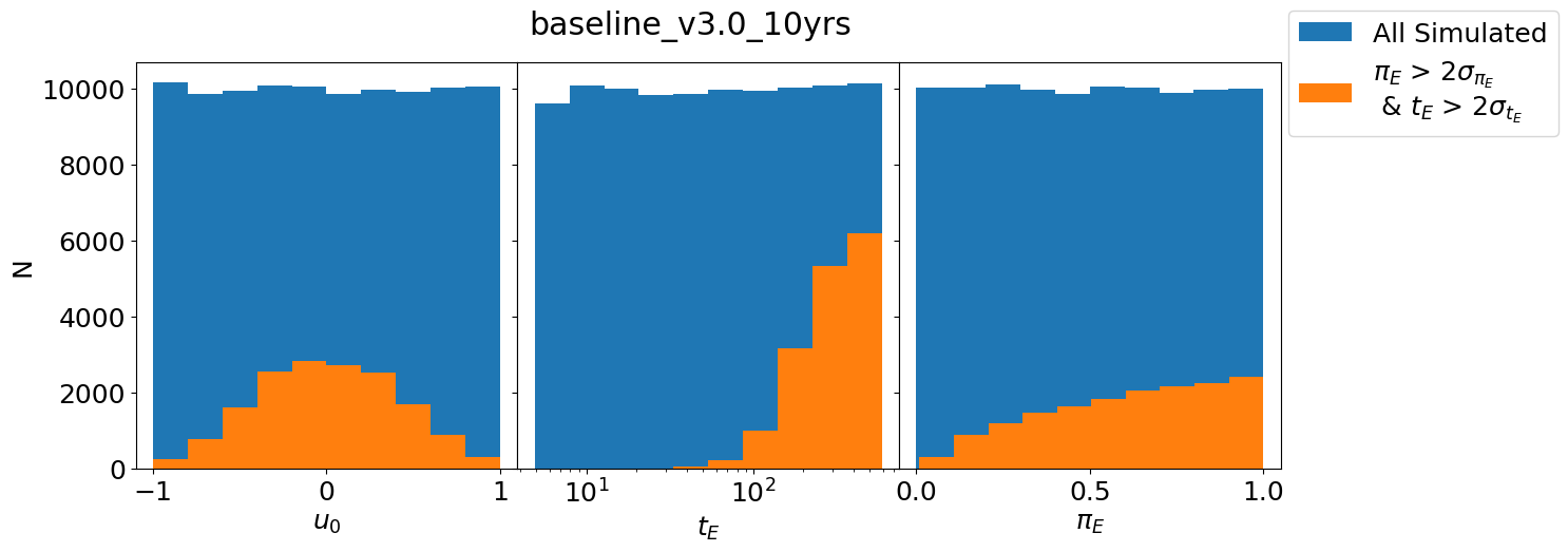
Figure 7: Distribution of $u_{0}$, $t_{\rm E}$, and $\pi_{\rm E}$ for simulated and characterized events. In blue are all of the simulated events and in orange are those that are characterized ($\pi_{\rm E}>2\sigma_{\pi_{\rm E}}$ and $t_{\rm E}>2\sigma_{t_{\rm E}}$) by the baseline_v3.0 OpSim in the bulge field RA = 263.89^∘, Dec = $-27.16^{\circ}$.

In this section we explore the characterizability of events with a microlensing parallax signal as described in Section 2.3. In Figure 7, we show a histogram of simulated (blue) and characterized (orange) event parameters. This is for the baseline_v3.0_10yrs in a field around RA = 263.89^∘, Dec = $-27.16^{\circ}$. We see those with smaller $|u_{0}|$ are characterized more easily due to their higher magnification. Longer $t_{\rm E}$ are characterized more frequently since events with longer $t_{\rm E}$ are more likely to be covered eventually. Large $\pi_{\rm E}$ are characterized more frequently due to the larger measurable signal.

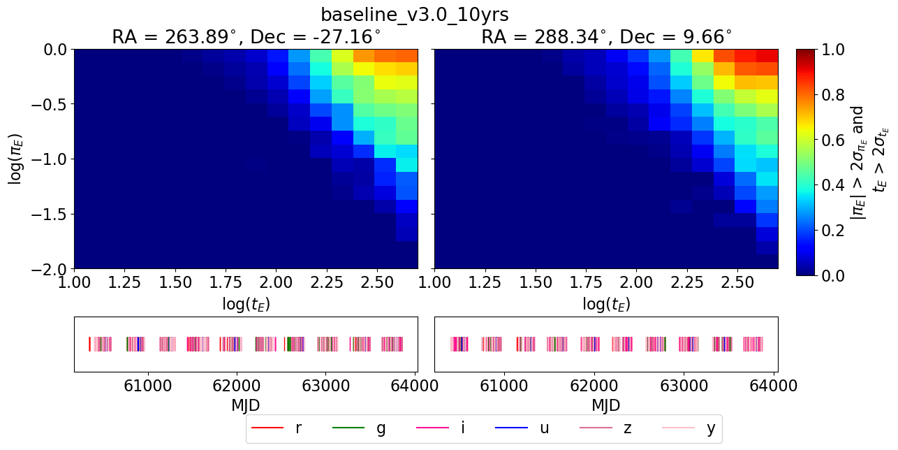
Figure 8: 2D-histogram of the fraction of events that are characterized for any given $t_{\rm E}$ and $\pi_{\rm E}$. Bluer squares have a lower fraction of characterized events and red have a higher fraction characterized. The bottom plots show the cadence of observations where different colors represent different filters, as indicated in the legend, for the given OpSim in a $3.5^{\circ}\times 3.5^{\circ}$ square centered on the RA and Dec indicated in the title of the left and right plots. Left is a representative bulge field and right is a representative disk field in a pencil beam. Due to the relatively faint baseline magnitudes as described in Section 2.2, there are very few events characterized with short $t_{\rm E}$ and small $\pi_{\rm E}$, but this does not mean that in general we cannot characterize events with these parameters with a realistic baseline magnitude distribution (see Figure 13). This plot is intended to be compared with Figures 9-12. See Figure 1 for a realistic distribution of simulated events in $\pi_{\rm E}-t_{\rm E}$ space.

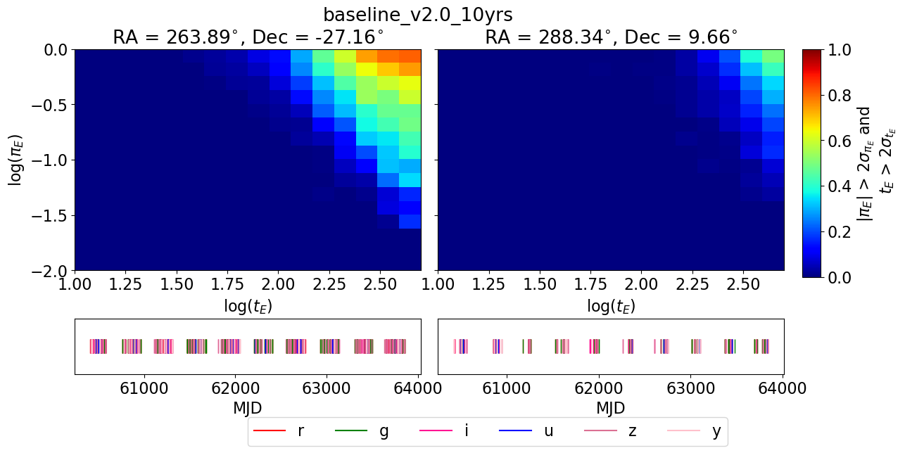
Figure 9: Same as 8 but for baseline_v2.0_10yrs. This footprint mostly focused on the Galactic bulge and neglected the plane. Hence the bulge field is better characterized on the 5-10% level and the disk field is $\sim$ 40% less characterized than baseline_v3.0_10yrs.

Figure 10: Same as Figure 8 but for rolling_all_sky_ns2_rw0.9_v2.0_10yrs. This OpSim has the same footprint as baseline_v2.0_10yrs but with rolling. While this does not explicitly roll the Galactic plane, the population in the bulge is characterized $\sim$10% less than baseline_v2.0_10yrs.

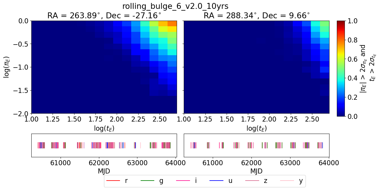
Figure 11: Same as Figure 8 but for rolling_bulge_6_v2.0_10yrs. This has the same footprint as baseline_v2.0_10yrs, but splits the bulge into six sections on which it alternates focus, as can be seen in the lower left panel. This leads to a worse characterization on the 15% level.

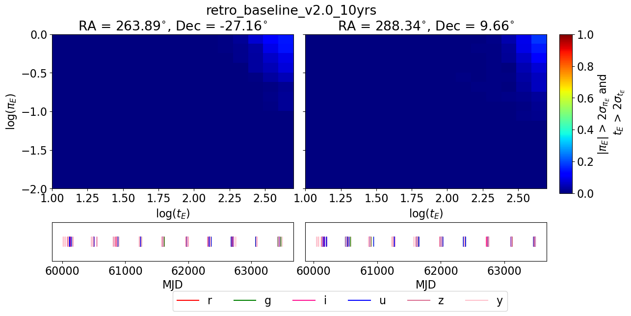
Figure 12: Same as Figure 8 but for retro_baseline_v2.0_10yrs. Given the extremely sparse cadence in the Galactic bulge and plane in the retro baseline, it would be 60-80% more difficult to characterize microlensing events.

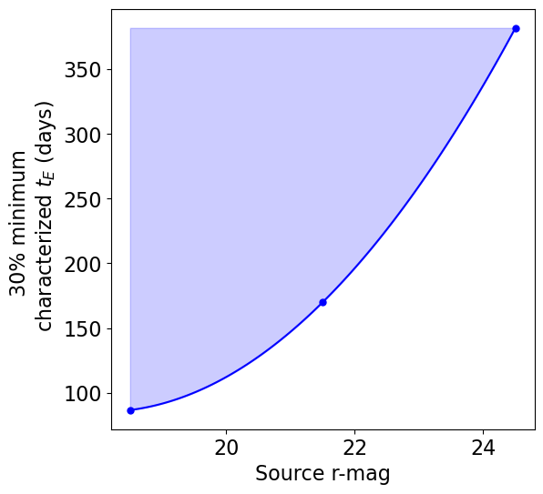
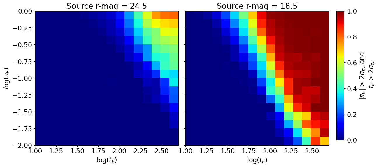
Figure 13: Left plots the minimum $t_{\rm E}$ for which 30% of events with $\pi_{\rm E}=0.1\pm 0.03$ for a given source r-mag. The shaded region represents areas where more than 30% of events with those parameters will be characterized. An r-mag = 24.5 corresponds to the default source magnitudes (see Section 2.2); an r-mag = 21.5 corresponds to decreasing all the source magnitudes by 3; and an r-mag = 18.5 corresponds to decreasing all the source magnitudes by 6. Middle is a 2D-histogram of $\pi_{\rm E}-t_{\rm E}$ for a bulge patch with the default source magnitudes; it is identical to the upper left plot in Figure 8. Right is the same as the middle panel but the default source magnitudes are all brighter by 6 magnitudes. For brighter stars, we are able to characterize events with shorter $t_{\rm E}$ and smaller $\pi_{\rm E}$.

In Figures 8-12, we plot 2D-histograms of $log(\pi_{\rm E}$) vs log($t_{\rm E}$) normalized by the number of events simulated in each square. In the lower panel, we plot the cadence of observations for that OpSim and field, where lines of different colors represent observations taken with different filters, as indicated by the legend. The left plot in each figure is for a representative bulge field and the right plot in each figure is for a representative disk field in a pencil beam field. Most events fall to the left side of these plots, see Figure 1 for a realistic distribution of simulated events in $\pi_{\rm E}-t_{\rm E}$ space.

In Figure 8, we can see that there are more characterizable events in the disk than in the bulge fields. The results show that this difference is $\sim 10-15\%$ which is due to the disk field having 10% more observations than the bulge field. Between baseline_v2.0_10yrs (Figure 9) and baseline_v3.0_10yrs (Figure 8) we can see there is a drop in the fraction of characterizable events. The results show this difference is at the 5-10% level for the bulge field. However, in the disk there is an improvement in characterization by as much as 50%. This is because in baseline_v3.0_10yrs there are more observations spread out across the plane, maximizing Rubin’s capability to do a Galaxy-wide study.

We can compare baseline_v2.0_10yrs to the rolling cadences since they share the same footprint. In rolling_all_sky_ns2_rw0.9_v2.0_10yrs (Figure 10), there is a drop in characterization efficiency on the 5-10% level due to longer periods with long gaps between observations. Whereas in rolling_bulge_6_v2.0_10yrs (Figure 11) there is a drop by $\sim 15-20\%$, particularly for high parallax events due to seasons with very sparse coverage and long gaps. In both, there is little change in the disk field as it has such sparse cadence and is not substantially rolled.

For reference, we can compare these cadences to retro_baseline_v2.0_10yrs (Figure 12). This covers the Galactic bulge and plane very sparsely and causes events to be 60-80% more difficult to characterize than the current baseline. This is indicative that the strongest determiner of characterization is the footprint. If time is not dedicated to the Galactic plane and bulge, most events will not be characterizable.

These results were all for the fixed baseline magnitude near Rubin’s limiting magnitude (see Section 2.2). In Figure 13, we explore how the characterization fraction changes with a decreasing source magnitude. We repeat the simulation decreasing the source magnitude in each filter by 3 and by 6, thereby making them brighter. We can see that we are able to characterize events with shorter $t_{\rm E}$ and smaller $\pi_{\rm E}$ when doing so. In the left panel of Figure 13, we have selected simulated events with $\pi_{\rm{}_{E}}=0.1\pm 0.03$ (the bulk of microlensing events) and determined the minimum $t_{\rm E}$ where 30% of the population is characterized. The shaded region represents areas where more than 30% of the population will be characterized. In the middle and right panels we compare the 2D-histogram of $\pi_{\rm E}-t_{\rm E}$ of the default (middle) and brighter magnitudes by 6 (right). We see that with events with brighter baseline magnitudes we are able to characterize events with shorter $t_{\rm E}$ and smaller $\pi_{\rm E}$.

4 Discussion and Conclusion

The main survey cadence optimizations that have a major effect on microlensing discovery and characterization can be summarized as followed.

1. Footprint, on the first order, makes the most significant impact on microlensing detection and characterization. This can be seen by comparing the current baselines to the “retro baseline” (see Figure 4).

2. Rubin will be able to use its uniquely deep and wide survey area to detect and characterize microlensing events across the Galactic plane. However, if areas of low stellar density and high extinction are included, this can lead to a decrease in the fraction of characterized events (see Figure 6).

3. Rolling in the Galactic bulge and plane has the potential to improve synergies with Roman, but should be approached with caution. The survey should avoid long gaps, since many current rolling strategies decrease detection and characterization of most microlensing events.

The survey cadences besides the “retro” footprints have also incorporated the LMC and SMC. Their inclusion will allow us to probe microlensing events cause by objects in the Galactic halo.

This paper has mostly discussed what Rubin can do alone with cadence optimization. Rubin will also send out nightly alerts which could be used to do follow-up on candidates and is of particular interest to exoplanet science. Follow-up observations could fill in gaps in Rubin’s coverage, but Rubin would still require adequate cadence in the wings of the event to reliably alert on events in progress. It may also be difficult to follow-up most faint events from most ground based facilities.

4.1 End-to-End Pipeline

The above assessment of cadence strategy has all been relative between cadences. We have simulated ranges of microlensing parameters such as $t_{\rm E}$ and $\pi_{\rm E}$ or plotted results as a function of those values. We have not incorporated a Galactic model and simulated a microlensing survey, which is necessary for predicting a realistic number and distribution of detected and characterized microlensing events.

Beyond the cadence, the pipeline, both reduction and analysis, will also play a large part in detection and characterization of microlensing events. We have seen with the first 3 years of Zwicky Transient Facility data, another all-visible-sky survey, covering one hemisphere, that $\sim 100$ events were discovered (Rodriguez et al., 2022; Medford et al., 2023). In order to find a pure sample, many real microlensing events were likely excluded due to the $>10^{9}$ initial lightcurves requiring strict cuts to fit all of the events (see Medford et al. (2023), Section 6). The analysis pipeline will have a significant effect on the microlensing yield. Given that microlensing is more likely to occur in crowded fields, carefully deblending and extracting photometry will be imperative to maximizing the number of detected and well characterized events. In a true end-to-end Rubin microlensing simulation, everything from initial physical Galactic parameters to reduction pipeline would be incorporated.

Since the Rubin Survey Optimization Committee plans to assess the cadence multiple times throughout Rubin’s operation, it is important to continue to develop our ability to assess cadences, including folding in real data.

Figures 14 and 15 summarize other select OpSims discussed in the paper, but without dedicated plots. Figure 14 has v2.0 OpSims and Figure 15 has v2.1-v3.0 OpSims. In Table 2, the OpSims discussed in this paper are summarized with descriptions relevant to microlensing and other Galactic science. See Jones et al. (2020) and Rubin technical note PSTN-055 for more detailed descriptions.

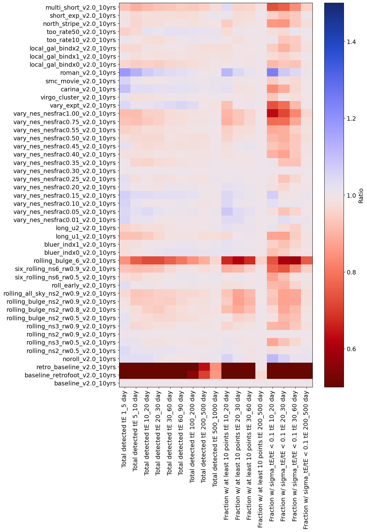
Figure 14: Same as Figure 4, but for select other v2.0 metrics, with baseline metrics for reference. This has the OpSims on the y-axis and the metrics on the x-axis for ease of plotting.

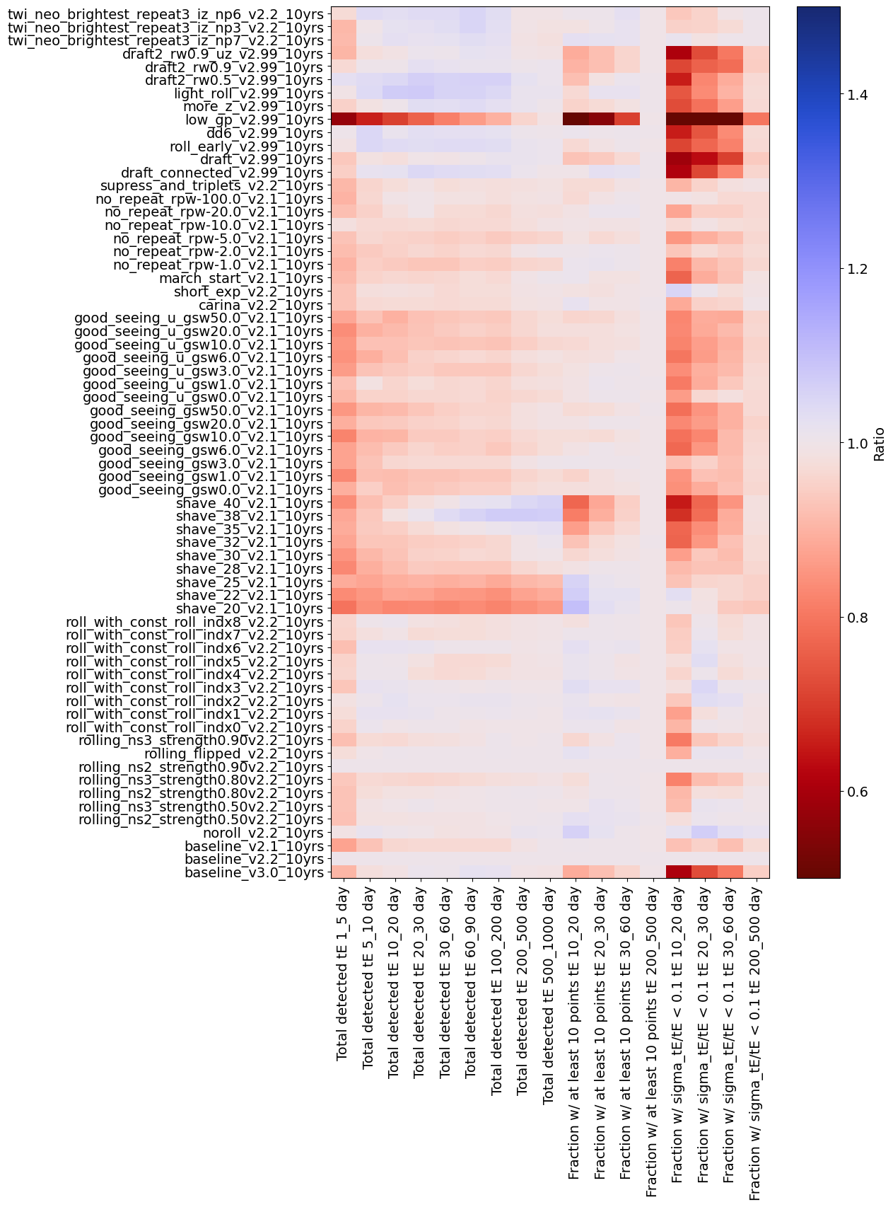
Figure 15: Same as Figure 4, but for select other 2.1 and later metrics, with baseline metrics for reference. All OpSims are plotted in refrence to baseline_v2.2_10yrs in this plot. A representative 3 of the 84 twilight_neo runs are plotted. This has the OpSims on the y-axis and the metrics on the x-axis for ease of plotting.

OpSim (Family) Name	Description
baseline	Baseline survey strategies.
baseline_v3.0_10yrs	Includes high priority areas across the Galactic plane and bulge.
baseline_v2.2_10yrs	Optimizations to code and DDF strategy change.
baseline_v2.1_10yrs	Includes Virgo cluster and acquisition of good seeing images in r and i bands.
baseline_v2.0_10yrs	Added in the Galactic bulge, LMC, and SMC.
baseline_retrofoot_v2.0_10yrs	Uses 2018 footprint and v2.0 baseline strategy.
retro_baseline_v2.0_10yrs	Uses 2018 footprint and strategy.
bluer_	Simulates different filter distributions, based on v2.0
ddf_	Varies survey strategy of DDFs.
galactic plane	Simulations that explore the Galactic plane survey strategy.
galplane_priority_	Varies Galactic footprint (1.5 is larger and 2.0 is smaller) and filter balance (bluer or redder).
plane_priority_priorityX_pbf_	Includes regions of Galactic plane with priority $\geq$ X not including pencil beam fields.
plane_priority_priorityX_pbt_	Includes regions of Galactic plane with priority $\geq$ X including pencil beam fields.
pencil_fsX_10yrs	Varies size/number of pencil beams where X = 1 is 20 smaller fields and X = 2 is 4 larger ones.
vary_gp_gpfracX_	Spends X% of survey time on areas of the Galactic plane not including in the WFD.
good_seeing_	Adds requirement of at least 3 good seeing images per year per pointing.
long_u_	u-band visits increased to 50s exposures.
microsurveys	Surveys requiring $<3\%$ of LSST time.
roman_v2.0_10yrs	Adds microsurvey of Roman GBTDS field.
smc_movie_v2.0_10yrs	Add two nights of observing of the SMC.
rolling	Varies strategy to alternate high cadence coverage of areas of the sky.
noroll_v2.0_10yrs	No rolling.
rolling_nsX_rwY_	Splits the sky into X regions with Y% strength of rolling.
rolling_bulge_nsX_rwY_	Splits the Galactic bulge into X regions with Y% strength of rolling.
rolling_early_v2.0_10yrs	Rolls beginning in year one of LSST.
six_rolling_	Splits sky into six regions and rolls.
rolling_bulge_6_v2.0_10yrs	Splits Galactic bulge into six regions and rolls.
rolling_with_const_	Interspurses rolling with constant years.
rolling_flipped_	Flips the order of the 2-band 90% strength rolling cadence.
triplets	Triplet observations in a single night strategies.
preseto_gapX	Triplets spaced X hours apart.
preseto_half_gapX	Triplets spaced X hours apart every other night.
long_gaps_nightsoffX_	Triplets every X nights.
long_gaps_nightsoffX_delayed_	Triplets every X nights starting after year 5.
twilight NEO	Survey added in twilight to observe Near Earth Objects.
vary expt	Strategies that vary the exposure time
vary_expt_	Varies the exposure time between 20 and 100 seconds.
shave_X	Changes exposure time to X seconds.
vary_NES_nesfracX_	Survey strategy spends X% of survey time on the North Ecliptic Spur.

Table 2: Summary of OpSims alphabetical by family that are relevant to microlensing and Milky Way science with descriptions of pertinent aspects. Those that end in an underscore indicate there are multiple OpSims related to that entry. Indented entries belong to the family listed above. See Jones et al. (2020) and Rubin technical note PSTN-055 for more detailed descriptions.

References

- Albrecht et al. (2006) Albrecht, A., Bernstein, G., Cahn, R., et al. 2006, arXiv e-prints, astro, doi: 10.48550/arXiv.astro-ph/0609591
- Alcock et al. (2000) Alcock, C., Allsman, R. A., Alves, D. R., et al. 2000, ApJ, 542, 281, doi: 10.1086/309512
- Bianco et al. (2019) Bianco, F. B., Drout, M. R., Graham, M. L., et al. 2019, PASP, 131, 068002, doi: 10.1088/1538-3873/ab121a
- Bianco et al. (2022) Bianco, F. B., Ivezić, Ž., Jones, R. L., et al. 2022, ApJS, 258, 1, doi: 10.3847/1538-4365/ac3e72
- Connolly et al. (2014) Connolly, A. J., Angeli, G. Z., Chandrasekharan, S., et al. 2014, in Society of Photo-Optical Instrumentation Engineers (SPIE) Conference Series, Vol. 9150, Modeling, Systems Engineering, and Project Management for Astronomy VI, ed. G. Z. Angeli & P. Dierickx, 14, doi: 10.1117/12.2054953
- Dal Tio et al. (2022) Dal Tio, P., Pastorelli, G., Mazzi, A., et al. 2022, ApJS, 262, 22, doi: 10.3847/1538-4365/ac7be6
- Gaudi (2012) Gaudi, B. S. 2012, ARA&A, 50, 411, doi: 10.1146/annurev-astro-081811-125518
- Gould (1992) Gould, A. 1992, ApJ, 392, 442, doi: 10.1086/171443
- Harris et al. (2020) Harris, C. R., Millman, K. J., van der Walt, S. J., et al. 2020, Nature, 585, 357, doi: 10.1038/s41586-020-2649-2
- Hunter (2007) Hunter, J. D. 2007, Computing in Science & Engineering, 9, 90, doi: 10.1109/MCSE.2007.55
- Jones & Yoachim (2022) Jones, L., & Yoachim, P. 2022, Rubin Metric Analysis Framework, https://github.com/lsst/rubin_sim.git
- Jones et al. (2020) Jones, R. L., Yoachim, P., Ivezic, Z., Neilsen, E. H., & Ribeiro, T. 2020, Survey Strategy and Cadence Choices for the Vera C. Rubin Observatory Legacy Survey of Space and Time (LSST), v1.2, Zenodo, doi: 10.5281/zenodo.4048838
- Jones et al. (2014) Jones, R. L., Yoachim, P., Chandrasekharan, S., et al. 2014, in Society of Photo-Optical Instrumentation Engineers (SPIE) Conference Series, Vol. 9149, Observatory Operations: Strategies, Processes, and Systems V, ed. A. B. Peck, C. R. Benn, & R. L. Seaman, 91490B, doi: 10.1117/12.2056835
- Jungman et al. (1996) Jungman, G., Kamionkowski, M., Kosowsky, A., & Spergel, D. N. 1996, Phys. Rev. D, 54, 1332, doi: 10.1103/PhysRevD.54.1332
- Kim et al. (2018) Kim, D. J., Kim, H. W., Hwang, K. H., et al. 2018, AJ, 155, 76, doi: 10.3847/1538-3881/aaa47b
- Lam & Lu (2023) Lam, C. Y., & Lu, J. R. 2023, arXiv e-prints, arXiv:2308.03302, doi: 10.48550/arXiv.2308.03302
- Lam et al. (2020) Lam, C. Y., Lu, J. R., Hosek, Matthew W., J., Dawson, W. A., & Golovich, N. R. 2020, ApJ, 889, 31, doi: 10.3847/1538-4357/ab5fd3
- Lam et al. (2022) Lam, C. Y., Lu, J. R., Udalski, A., et al. 2022, ApJ, 933, L23, doi: 10.3847/2041-8213/ac7442
- Lam et al. (2023) Lam, C. Y., Abrams, N., Andrews, J., et al. 2023, arXiv e-prints, arXiv:2306.12514, doi: 10.48550/arXiv.2306.12514
- Lu et al. (2016) Lu, J. R., Sinukoff, E., Ofek, E. O., Udalski, A., & Kozlowski, S. 2016, ApJ, 830, 41, doi: 10.3847/0004-637X/830/1/41
- Medford et al. (2023) Medford, M. S., Abrams, N. S., Lu, J. R., Nugent, P., & Lam, C. Y. 2023, ApJ, 947, 24, doi: 10.3847/1538-4357/acba8f
- Meurer et al. (2017) Meurer, A., Smith, C. P., Paprocki, M., et al. 2017, PeerJ Computer Science, 3, e103, doi: 10.7717/peerj-cs.103
- Moniez (2010) Moniez, M. 2010, General Relativity and Gravitation, 42, 2047, doi: 10.1007/s10714-009-0925-4
- Moniez et al. (2017) Moniez, M., Sajadian, S., Karami, M., Rahvar, S., & Ansari, R. 2017, A&A, 604, A124, doi: 10.1051/0004-6361/201730488
- Mróz et al. (2022) Mróz, P., Udalski, A., & Gould, A. 2022, ApJ, 937, L24, doi: 10.3847/2041-8213/ac90bb
- Naghib et al. (2019) Naghib, E., Yoachim, P., Vanderbei, R. J., Connolly, A. J., & Jones, R. L. 2019, AJ, 157, 151, doi: 10.3847/1538-3881/aafece
- Paczynski (1986) Paczynski, B. 1986, ApJ, 304, 1, doi: 10.1086/164140
- Rodriguez et al. (2022) Rodriguez, A. C., Mróz, P., Kulkarni, S. R., et al. 2022, ApJ, 927, 150, doi: 10.3847/1538-4357/ac51cc
- Sahu et al. (2022) Sahu, K. C., Anderson, J., Casertano, S., et al. 2022, ApJ, 933, 83, doi: 10.3847/1538-4357/ac739e
- Sajadian & Poleski (2019) Sajadian, S., & Poleski, R. 2019, ApJ, 871, 205, doi: 10.3847/1538-4357/aafa1d
- Spergel et al. (2015) Spergel, D., Gehrels, N., Baltay, C., et al. 2015, arXiv e-prints, arXiv:1503.03757, doi: 10.48550/arXiv.1503.03757
- Street et al. (2018) Street, R., Lund, M., Khakpash, S., et al. 2018, arXiv preprint arXiv:1812.03137
- Street et al. (2023a) Street, R. A., Li, X., Khakpash, S., et al. 2023a, ApJS, 267, 15, doi: 10.3847/1538-4365/acd6f4
- Street et al. (2023b) Street, R. A., Gough-Kelly, S., Lam, C., et al. 2023b, arXiv e-prints, arXiv:2306.13792, doi: 10.48550/arXiv.2306.13792
- Sumi et al. (2003) Sumi, T., Abe, F., Bond, I. A., et al. 2003, ApJ, 591, 204, doi: 10.1086/375212
- Tsapras et al. (2016) Tsapras, Y., Hundertmark, M., Wyrzykowski, Ł., et al. 2016, MNRAS, 457, 1320, doi: 10.1093/mnras/stw023
- Udalski et al. (2015) Udalski, A., Szymański, M. K., & Szymański, G. 2015, Acta Astron., 65, 1, doi: 10.48550/arXiv.1504.05966
- Yee et al. (2014) Yee, J. C., Albrow, M., Barry, R. K., et al. 2014, arXiv e-prints, arXiv:1409.2759, doi: 10.48550/arXiv.1409.2759