NRCPS-HE-70-2023

Caustics in Self-gravitating N-body systems
and
Large Scale Structure of Universe

George Savvidy

Institute of Nuclear and Particle Physics

Demokritos National Research Center, Ag. Paraskevi, Athens, Greece

Abstract

In this paper we demonstrate the generation of gravitational caustics that appear due to the geodesic focusing in a self-gravitating N-body system. The gravitational caustics are space regions where the density of particles is higher than the average density in the surrounding space. It is suggested that the intrinsic mechanism of caustics generation is responsible for the formation of the cosmological Large Scale Structure that consists of matter concentrations in the form of galaxies, galactic clusters, filaments, and vast regions devoid of galaxies.

In our approach the dynamics of a self-gravitating N-body system is formulated in terms of a geodesic flow on a curved Riemannian manifold of dimension 3N equipped by the Maupertuis’s metric. We investigate the sign of the sectional curvatures that defines the stability of geodesic trajectories in different parts of the phase space. The regions of negative sectional curvatures are responsible for the exponential instability of geodesic trajectories, deterministic chaos and relaxation phenomena of globular clusters and galaxies, while the regions of positive sectional curvatures are responsible for the gravitational geodesic focusing and generation of caustics. By solving the Jacobi and the Raychaudhuri equations we estimated the characteristic time scale of generation of gravitational caustics, calculated the density contrast on the caustics and compared it with the density contrasts generated by the Jeans-Bonnor-Lifshitz-Khalatnikov gravitational instability and that of the spherical top-hat model of Gunn and Gott.

1 Introduction

Galaxies are not distributed uniformly in space and time, as it can be seen in Fig. 1 and Fig. 2 representing the data of the Sloan Digital Sky Survey [1, 2, 3] and of the Dark Energy Spectroscopic Instrument collaboration [4, 5, 6]. Extended galaxy redshift surveys revealed that at a large-scale the Universe consists of matter concentrations in the form of galaxies and clusters of galaxies of Mpc scale, as well as filaments of galaxies that are larger than 10 Mpc in length and vast regions devoid of galaxies [1, 2, 3, 4, 5, 6, 7, 8, 9, 10, 11, 12, 13, 14]. The JWST telescope [15] and the Euclid mission [12] will observe the first stars and galaxies that formed in the Universe from the epoch of recombination to the present day. The Large Scale Structure (LSS) of the Universe is this pattern of galaxies that provides information about the spectrum of matter density fluctuations shown in Fig. 3 .

The prevailing theoretical paradigm regarding the existence of LSS is that the initial density fluctuations of the early Universe seen as temperature deviations in the Cosmic Microwave Background (CMB) grow through gravitational instability into the structure seen today in the galaxy density field [13, 14, 16, 17, 18, 19, 20, 21, 22, 23, 24, 25, 26, 27, 28, 29, 30, 31, 32, 33, 34, 35, 36, 37]. The best constraints on the matter density fluctuations come from the study of the CMB temperature fluctuations generated at the epoch of the last scattering of the radiation [7, 8, 9, 10, 11]. The LSS of galaxies provides independent measurements of density fluctuations of similar physical scale, but at the late epoch. The combination of CMB measurements with measurements of LSS provide independent probes of the matter power spectrum in complementary regions shown in Fig.3.

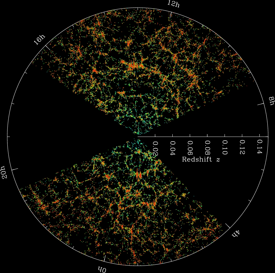
Figure 1: This figure shows galaxies discovered by the Sloan Digital Sky Survey (SDSS). Galaxy filaments forming the cosmic web consist of walls of gravitationally bound galactic superclusters that can be seen by eye. The figure shows galaxies up to around 2 billion light-years away (z=0.14). Figure Credit: M. Blanton and SDSS [1, 2, 3].

Our aim is to investigate the problem of LSS formation in terms of the nonlinear dynamics of a self-gravitating N-body system. This investigation is complementary to a fluid description of the cosmological N-body problem and numerical simulations that are commonly applied to this problem [13, 14, 16, 19, 17, 26, 27, 31, 32, 33, 34, 35, 36, 37, 38, 39, 40, 41, 42, 43, 44, 45, 46]. In our approach the Hamiltonian dynamics of N-body system is represented as the geodesic flow on the curved coordinate manifold $Q^{3N}$, and the nonlinear interaction is imprinted into the curvature structure of the Riemannian manifold $Q^{3N}$ [47]. This geometrisation of the N-body dynamics [47, 48, 49, 50, 51] allows to investigate the gravitational geodesic focusing and generation of caustics, the space regions where the density of particles is higher than the average density in the surrounding space.

The geometrisation of the Hamiltonian dynamics was initially developed and applied to the investigation of nonlinear dynamics of the Yang-Mills gauge field demonstrating that the Yang-Mills Classical Mechanics is a system of a deterministic chaos [47, 52, 53, 48, 49, 50, 54]. Subsequently the geometrisation method was applied to the investigation of the relaxation phenomenon in self-gravitating N-body systems [51]. In the present article we are further developing and extending this method in new directions in order to analyse the behaviour of the N-body system in the whole phase space of negative and positive sectional curvatures, investigating the gravitational geodesic focusing and the generation of caustics. Our approach allows to extend the ideas of Lifshitz, Khalatnikov, Zeldovich, Arnold, and other researchers [17, 20, 26, 28, 29, 30, 55, 56, 57] and to demonstrate the generation of caustics in self-gravitating N-body systems.

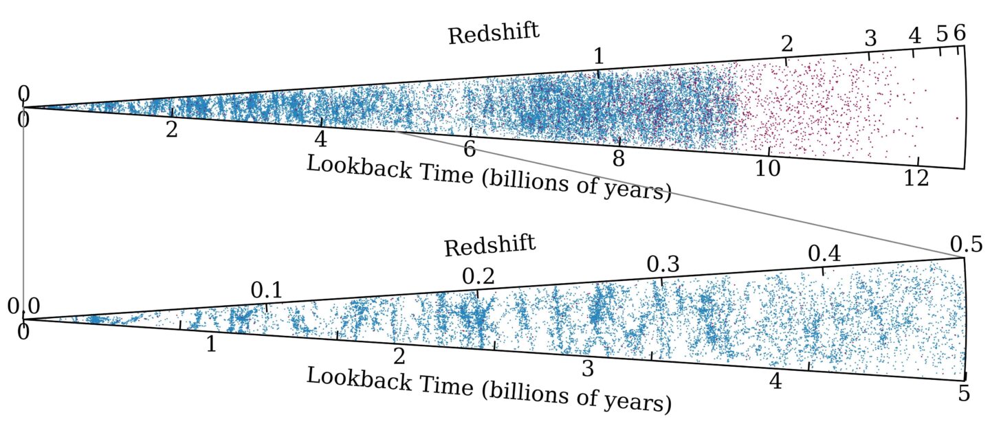
Figure 2: The space-time distribution of galaxies as a function of redshift. This DESI data has the Earth on the left and looks back in time to the right. Every dot represents a galaxy (blue) or quasar (red). The upper wedge includes objects all the way back to about 12 billion years ago. The bottom wedge zooms in on the closer galaxies in more detail. The clumps, strands, and blank spots are real structures in the Universe showing how galaxies group together or leave voids on gigantic scales. Figure Credit: Eleanor Downing/DESI collaboration [4, 5, 6] .

In this approach the ”particles” might represent standard particles and dark matter particles, stars, galaxies or clusters of galaxies interacting gravitationally. This formulation of the N-body dynamics allows to investigate the stability of geodesic trajectories by the Jacobi deviation equation and gravitational geodesic focusing, the generation of conjugate points and caustics by means of the Raychaudhuri equation. We will consider the physical conditions at which a self-gravitating system is developing geodesic focusing, conjugate points and caustics. Caustics are regions in the space where the density of particles is higher than the average density in the background space and therefore can represent galaxies, clusters of galaxies, filaments, and regions of lower density, voids, shown in Figs. 1, 2.

In order to study the stability of geodesic trajectories and the generation of caustics in the N-body systems one should know the properties of the sectional curvature $K(q,u,\delta q_{\perp})$ that is entering into the Jacobi equations. We investigate the sign of the sectional curvature $K(q,u,\delta q_{\perp})$ that defines the stability of geodesic trajectories in different parts of the phase space. $\alpha$) In the regions where the sectional curvature is negative the trajectories of particles are unstable, are exponentially diverging, and the self-gravitating system is in a phase of deterministic chaos. $\beta$) In the regions where the sectional curvature is positive the trajectories are stable, exhibit geodesic focusing, generating conjugate points and caustics. As it will be demonstrated in the forthcoming sections, a self-gravitating N-body system can be assigned to these distinguished regions of the phase space depending on the initial distribution of particles velocities and quadrupole momentum of the system. Our aim is to investigate these regions of the phase space and to pin-point these regions precisely.

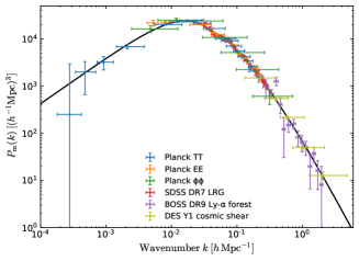
Figure 3: The matter power spectrum (at z = 0) inferred from different cosmological probes showing how CMB, LSS, clusters, weak lensing, and Ly$\alpha$F all constrain matter power spectrum $P(k)$ [11]. The spectrum measures the power of matter fluctuations on a given scale $k$. For the long wave length perturbations it has power-law behaviour $P(k)\propto k^{n_{s}}$ with the scalar spectral index $n_{s}=0.967\pm 0.004$, tilted away from the scale invariant $n_{s}=1$ Harisson-Zeldovich spectrum. The sound waves diminish the strength of small scale fluctuations, and power spectrum tends to fall as $P(k)\propto k^{-3}$ for $k\geq 2\times 10^{-2}[h~{}\text{Mps}^{-1}]$.

The article is organised as follows. In the second section we reformulate the dynamics of a self-gravitating N-body system in terms of a geodesic flow on a curved Riemannian manifold $Q^{3N}$ of dimension $3N$ equipped by the Maupertuis’s metric (2.8). This mapping allows to translate the N-body dynamics into the geometrical properties of the Riemannian manifold $Q^{3N}$, which are encoded in the corresponding Riemann tensor. It provides the geometrisation of the N-body dynamics and the application of geometrical concepts to the problem of relaxation phenomena and to the problem of gravitational geodesic focusing in self-gravitating N-body systems and generation of caustics. In Appendix A we prove that the corresponding Weyl tensor vanishes and that the Maupertuis’s metric is conformally flat. Due to this fact the Riemann tensor can be expressed in terms of Ricci tensor and scalar curvature. By using this representation (1.194) of the Riemann tensor we express the sectional curvatures (5.53), (5.55) appearing in the Jacobi equations (5.51), (5.52) and in (5) in terms of the Ricci tensor and scalar curvature (1.195).

In the third and forth sections we derive the Jacobi equation in the form that is more convenient for the investigation of N-body systems. In the fifth section we consider the projection of the Jacobi equation into a moving frame associated with the geodesic trajectories. This allows to transform the Jacobi equation written in terms of covariant derivative into the equation that is written in terms of ordinary derivatives. In the sixth, seventh and eighth sections we consider and define regions of the phase space of positive and negative sectional curvatures. The regions of negative sectional curvatures are responsible for the exponential instability of geodesic trajectories and for the chaotic behaviour of the system and the relaxation phenomena, while regions of the phase space of positive sectional curvatures are responsible for the gravitational geodesic focusing and generation of caustics, regions of space where the density of matter is larger than in the ambient space.

In the case of negative sectional curvatures we derived the Anosov inequality and the value of the maximal Lyapunov exponent of the diverging and converging foliations of trajectories and estimated the collective relaxation time of stars in galaxies, stars in globular clusters, and galaxies in galactic clusters. The subject of the relaxation time and evaporation is fundamental and was investigated by many authors including Rosseland [69], Ambartsumian [70], Spitzer [71], Chandrasekhar [72], Lynden-Bell [73, 74], King [75], and Gurzadian and Savvidy [51].

In the case of positive sectional curvatures we derived the physical conditions at which an N-body system is developing gravitational geodesic focusing and caustics. We estimated the time scale at which the spherically symmetric expansion of a self-gravitating system of particles/galaxies will contract into higher-density caustics, regions where particles/galaxies pile up into low-dimensional hypersurfaces and filaments. We found that the time scale of the appearance of gravitational caustics is

$$\tau_{caustics}=~{}{1\over 4\pi G\rho(t)}~{}{\dot{a}(t)\over a(t)}={1\over 4\pi G\rho(t)}H(t),$$ (1.1)

where $\rho(t)$ is a matter density and $H(t)$ is the Hubble parameter. This characteristic time scale of the generation of gravitational caustics demonstrates that the caustics appear very early in the history of the expanding Universe. This time scale for the matter-dominated epoch is

$$\tau_{caustics}=\alpha{2\over 3H(t)}=\alpha~{}t,$$ (1.2)

where $\alpha=\sqrt{9/10}$. The time required to generate gravitational caustics is considerably shorter at early stages of the Universe expansion at the recombination epoch and linearly increases with expansion. Considering the radiation-dominated epoch one can obtain the identical functional time dependence, with $\alpha=\sqrt{2/5}$. We compared this time scale of caustics generation with the Jeans-Bonnor-Lifshitz-Khalatnikov gravitational instability time scales [16, 17, 19, 20, 27] and that of the spherical top-hat model of Gunn and Gott [76].

In the ninth section we derive the Ranchandhuri equation (5.44) that describes the time evolution of the volume expansion scalar $\theta$ in the case of an N-body system that defines the contraction or expansion rates. The equation contains the quadratic form built in terms of the Ricci curvature tensor $R_{\alpha\beta}u^{\alpha}u^{\beta}$. By using the metric tensor, which is expressed in terms of orthonormal frame $\{u,\nu_{i}\}$, we obtained the representation of this quadratic form as a sum of sectional curvatures spanned by pairs of the velocity vector $u$ and all orthonormal frame vectors $\{\nu_{i}\}$ (9.142). We also derived a useful representation of the scalar curvature $R$ in terms of a sum of all sectional curvatures $K(u,\nu_{i})$ and $K(\nu_{i},\nu_{j})$ (9.138). Both relations make clear the crucial role of sectional curvatures in the evolution of dynamical systems.

In the tenth section we discuss the general conditions under which the geodesic focusing, the conjugate points and caustics are generated in dynamical systems. In the eleventh section we derive the condition under which the gravitational caustics are generated in a self-gravitating N-body system and estimate the time scale at which the network of caustics is generated during the expansion of the Universe. Considering the evolution of a self-gravitating N-body system occupying the initial volume ${\cal V}(0)$ we obtained the following expression for its proper time evolution:

$${\cal V}(s)={\cal V}(0)\Big{[}\cos\Big{(}{B\over 3N}s\Big{)}\Big{]}^{3N}.$$ (1.3)

The caustics are generated at each epoch $s_{caustic}={3\pi N\over 2B}(1+2n),n=0,\pm 1,\pm 2,...$, when the volume occupied by the particles is contracted to zero and the expansion scalar $\theta(s)$ is singular:

$$\theta(s)=-B\tan\Big{(}{B\over 3N}s\Big{)}.$$ (1.4)

The density contrast in the vicinity of a caustic has the following form:

$$\delta_{caustics}+1=\Big{[}\cos\Big{(}{B\over 3N}s\Big{)}\Big{]}^{-3N}.$$ (1.5)

The time scale of the appearance of the first caustic is given by $\tau_{caustics}$.

The behaviour of the matter power spectrum at small scales $k\geq 2\times 10^{-2}[h~{}\text{Mps}^{-1}]$ shown in Fig. 3 has a non-perturbative character and cannot be described by the perturbation theory because there the matter density contrast $\delta$ is large. The maximal density contrast that can be achieved in the spherical top-hat model of Gunn and Gott [76] is about $18\pi^{2}\approx 200$ (8.113). The density contrast in the vicinity of the caustics can be large enough to describe the spectrum of small scale perturbations. The region of small scale perturbations can be investigated by numerical simulations, and it would be interesting to compare the theoretical result (1.5) with the results obtained in numerical simulations of the density contrast and of that from the observational data. The derived formulas allow to investigate the sectional curvatures not only analytically but also in the numerical simulation of gravity. So we conclude that a radially expanding self-gravitating N-body system can develop gravitational caustics, surfaces and filaments in which the density of galaxies and galactic clusters is higher than the average density in the Universe.

2 Geometrisation of Self-Gravitating N-body System

By the geometrisation of N-body dynamics we mean the correspondence that maps and puts into the one-to-one correspondence the Euler-Lagrangian equation of interacting particles with the geodesic equation on the Riemannian manifold $Q^{3N}$, which is equipped by the Maupertuis-Euler-Jacobi metric [77, 78, 79]. The geometrisation of the N-body dynamics has a great advantage because it reduces the investigation of N-body dynamics to the investigation of the properties of geodesic flows on a Riemannian manifold. The geodesic flows on Riemannian manifolds is an intensive subject of research, and the methods that were developed in this field provide a powerful tool that allows to investigate the stability of the geodesic trajectories, the behaviour of the congruence of geodesic trajectories, conjugate points and caustics [58, 66, 67], investigate the intrinsic properties of the dynamical systems per se [80, 81, 82, 83, 84, 85, 86, 87]. The geometrical formulation of classical dynamics has a universal character and was applied to the investigation of nonlinear dynamics of Yang-Mills field and self-gravitating N-body systems [47, 49, 50, 53, 48, 54, 51, 88, 89].

Let us consider a system of $N$ massive particles with masses $M_{\alpha}$ and the coordinates

$$q^{\alpha}(s)=(M^{1/2}_{1}\vec{r_{1}},...,M^{1/2}_{N}\vec{r_{N}}),~{}~{}~{}\alpha=1,...,3N,$$ (2.6)

that are defined on a Riemannian coordinate manifold $q^{\alpha}(s)\in Q^{3N}$ and have the velocity vector

$$u^{\alpha}(s)={dq^{\alpha}\over ds},~{}$$ (2.7)

where $s$ is the proper time parameter along the trajectory $\gamma(s)$ in the coordinate manifold $Q^{3N}$. It is fundamentally important that the definition of the coordinates $q^{\alpha}$ includes the masses of the particles. The conformally flat Maupertuis’s metric on $Q^{3N}$ is defined as [77, 78, 79, 86, 47, 51]

$$ds^{2}=g_{\alpha\beta}dq^{\alpha}dq^{\beta},~{}~{}~{}~{}g_{\alpha\beta}=\delta_{\alpha\beta}(E-U(q))=\delta_{\alpha\beta}W(q),$$ (2.8)

where particles are interacting through the potential $U(q)$ (see Appendix A). An N-body system can be in a background field of the expanding Universe and in that case the potential function will contain an additional part that describes the background potential that influences the motion of the particles in a background field. Due to the proper time parametrisation of the trajectories it follows from (2.7) and (2.8) that the velocity vector is of a unit length:

$$g_{\alpha\beta}u^{\alpha}u^{\beta}=1.$$ (2.9)

The resulting phase space manifold $(q,u)\in W^{6N-1}$ has a bundle structure with the base $q\in Q^{3N}$ and the (3N-1)-dimensional spheres $S^{3N-1}$ of unit tangent vectors $u^{\alpha}$ (2.9) as fibers. The geodesic trajectories on the Riemannian manifold $Q^{3N}$ are defined by the following equation:

$${d^{2}q^{\alpha}\over ds^{2}}+\Gamma^{\alpha}_{\beta\gamma}{dq^{\beta}\over ds}{dq^{\gamma}\over ds}=0,$$ (2.10)

where the Christoffel symbol $\Gamma^{\lambda}_{\alpha\beta}$ denotes the torsion-free connection on $Q^{3N}$. Let us demonstrate that the geodesic equation (2.10) coincides with the Euler-Lagrangian equation for the particles that are interacting through the potential $U(q)$ in (2.8). Contracting the Christoffel symbols $\Gamma^{\alpha}_{\beta\gamma}$ with the velocity vectors $u^{\alpha}$ in (2.10) will yield

$$\Gamma^{\alpha}_{\beta\gamma}u^{\beta}u^{\gamma}={1\over 2}g^{\alpha\delta}\Big{(}{\partial g_{\delta\beta}\over\partial q^{\gamma}}+{\partial g_{\delta\gamma}\over\partial q^{\beta}}-{\partial g_{\beta\gamma}\over\partial q^{\delta}}\Big{)}u^{\beta}u^{\gamma}={1\over W}\Big{(}u^{\alpha}{\partial W\over\partial q^{\beta}}u^{\beta}-{1\over 2}g^{\alpha\beta}{\partial W\over\partial q^{\beta}}\Big{)},$$

thus the geodesic equation (2.10) reduces to the following form:

$${d^{2}q^{\alpha}\over ds^{2}}+{1\over W}\Big{(}u^{\alpha}{\partial W\over\partial q^{\beta}}u^{\beta}-{1\over 2}g^{\alpha\beta}{\partial W\over\partial q^{\beta}}\Big{)}=0.$$ (2.11)

The physical time variable $t$ should be introduced by the relation

$$ds=\sqrt{2}Wdt,$$ (2.12)

and for the velocity vector we will have

$$u^{\alpha}={1\over\sqrt{2}W}(M^{1/2}_{1}{d\vec{r}_{1}\over dt},...,M^{1/2}_{N}{d\vec{r}_{N}\over dt}).$$ (2.13)

By transforming the second derivative in the last equation into the physical time one can obtain the following equation:

$${d^{2}q^{\alpha}\over dt^{2}}-Wg^{\alpha\beta}{\partial W\over\partial q^{\beta}}~{}=~{}{d^{2}q^{\alpha}\over dt^{2}}+{\partial U\over\partial q^{\alpha}}=0.$$

In terms of the coordinate system (2.6) introduced above ($\vec{r}_{a},~{}a=1,...,N$) this equation reduces to the Euler-Lagrangian equation for massive particles interacting though the potential function $U(\vec{r}_{1},...,\vec{r}_{N})$:

$$M_{a}{d^{2}\vec{r}_{a}\over dt^{2}}=-{\partial U\over\partial\vec{r}_{a}},~{}~{}~{}~{}~{}~{}~{}a=1,...,N.$$ (2.14)

Thus the N-body dynamics that is described by the Euler-Lagrangian equation (2.14) is put into the one-to-one correspondence with the geodesic equation (2.10) on the Riemannian manifold $Q^{3N}$ supplied by the metric (2.8) and therefore allows to investigate the stability of the geodesic trajectories, the behaviour of a congruence of trajectories, the conjugate points and caustics in terms of the geometrical properties of the Riemannian manifold $Q^{3N}$.

Thus the classical dynamics of the interaction particles in a flat space-time can be reformulated in terms a free motion of particles moving along the geodesic trajectories in a curved space-time [82, 81, 80, 83, 84, 85, 86, 87, 49, 50]. The local and global properties of the geodesic trajectories strongly depend on the properties of the Riemannian curvature tensor and of the sectional curvatures. Indeed, the behaviour of a congruence of geodesic trajectories is described by the Jacobi deviation equation, and the appearance of conjugate points and caustics is described by the Raychaudhuri equation [58, 66, 67]. In the Jacobi deviation equations it is the sectional curvature that plays a dominant role, while in the Raychaudhuri equation the Ricci tensor is doing so. In this respect the curvature tensors play a fundamental role in both equations, and they will be defined and investigated in the forthcoming sections. The relation between the Riemann and Ricci curvature tensors and the Weyl tensor in the case of Maupertuis’s metric (2.8) is considered in Appendix A. In the next section we will calculate these tensors in the case of a manifold that is equipped with the Maupertuis’s metric (2.8).

3 Jacobi Equation for Deviation Vector

Let us consider a smooth curve $\gamma(s)$ with coordinates $q^{\alpha}(s)=(M^{1/2}_{1}\vec{r_{1}},...,M^{1/2}_{N}\vec{r_{N}})$ in $Q^{3N}$ describing collectively the trajectory of N particles and having the velocity vector $u^{\alpha}(s)$ (2.7). The masses $M_{\alpha}$ can represent the masses of particles or the masses of stars, of galaxies or of clusters of galaxies. The covariant derivative on the coordinate manifold $Q^{3N}$ is defined as

$$Du^{\alpha}=du^{\alpha}+\Gamma^{\alpha}_{\beta\gamma}u^{\beta}dq^{\gamma},~{}~{}~{}{Du^{\alpha}\over ds}=({\partial u^{\alpha}\over\partial q^{\beta}}+\Gamma^{\alpha}_{\beta\gamma}u^{\gamma})u^{\beta}\equiv u^{\alpha}_{~{};\beta}u^{\beta},$$ (3.15)

under which the metric (2.8) is covariantly constant and under which the scalar product

$$(u\cdot v)\equiv g_{\alpha\beta}u^{\alpha}v^{\beta}$$ (3.16)

is preserved along a smooth curve $\gamma(s)$ when the vectors $u^{\alpha}$ and $v^{\beta}$ are parallelly transported along $\gamma(s)$, that is, $Du^{\alpha}=0,~{}Dv^{\beta}=0$. Differentiating the relation (2.9) we will get the equation

$$u^{\alpha}u_{\alpha;\beta}=0$$ (3.17)

expressing the orthogonality of the acceleration tensor $u_{\alpha;\beta}$ to the velocity vector $u^{\alpha}$ at every point of the curve $\gamma(s)$. The geodesic equation of motion (2.10) for the particles that are interacting through the potential $U(q)$ can be expressed in terms of the covariant derivative:

$${Du^{\alpha}\over ds} = {d^{2}q^{\alpha}\over ds^{2}}+\Gamma^{\alpha}_{\beta\gamma}{dq^{\beta}\over ds}{dq^{\gamma}\over ds}=u^{\alpha}_{~{};\beta}u^{\beta}=0.$$ (3.18)

From equations (3.17) and (3.18) it follows that on the geodesic trajectories the acceleration tensor $u_{\alpha;\beta}$ lies in a hypersurface $\Sigma_{\perp}$, which is orthogonal to the velocity vector $u^{\alpha}$ (see Fig.4):

$$u^{\alpha}u_{\alpha;\beta}=0,~{}~{}~{}~{}u_{\alpha;\beta}u^{\beta}=0.$$ (3.19)

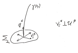
Figure 4: As it follows from the equations (3.17) and (3.18) the acceleration tensor $u_{\alpha;\beta}$ lies in the hypersurface $\Sigma_{\perp}$, which is orthogonal to the tangent velocity vector $u^{\alpha}$. The figure shows the tangent vector $u^{\alpha}$ and the orthogonal hypersurface $\Sigma_{\perp}$. The $\nu^{\alpha}_{i}$ are the orthonormal frame vectors $\nu^{\alpha}_{i}\nu_{j\alpha}=\delta_{ij}$ perpendicular to the velocity vector $u_{\alpha}\nu^{\alpha}_{i}=0.$ They define the orthonormal frame $\{u,\nu_{i}\}$ along the curve $\gamma(s)$ (5.35).

Let us consider a one-parameter family of curves $\{\gamma(s,\upsilon)\}$ in the neighbourhood of the curve $\gamma(s)$ assumed to form a congruence [80, 66, 67]. In order to characterise a congruence of curves $\{\gamma(s,\upsilon)\}$ around $\gamma(s)$ it is convenient to consider a smooth one-parameter family of curves $\gamma(s,v)$:

$$q^{\alpha}(s)\rightarrow q^{\alpha}(s,\upsilon)$$ (3.20)

describing the relation between the curve $\gamma(s)$ and curves that lie infinitesimally close to it. Each curve of the congruence $\{\gamma(s,\upsilon)\}$ is defined by setting $\upsilon=constant$, and $\gamma(s)$ is given by $\upsilon=0$. One can imagine these curves as representing the flow lines of a perfect fluid, and we are interested in the rate at which the velocity, shear and expansion of such family of curves are changing during the time evolution of the fluid. The deviation is defined as

$$\delta q^{\alpha}={\partial q^{\alpha}\over\partial\upsilon}d\upsilon,$$ (3.21)

therefore $\delta q^{\alpha}$ is a separation of points having equal distance from some initial points along two neighbouring curves (see Fig.5). In other words, the vector $\delta q^{\alpha}$ connects points of $\gamma$ to corresponding points of some neighbouring curve $\gamma^{{}^{\prime}}$ and describes the behaviour of the curves in an infinitesimal neighbourhood of a given curve $\gamma(s)$. One can calculate the covariant derivative of the deviation vector $\delta q^{\alpha}$ as

$${D\delta q^{\alpha}\over ds}={\partial\delta q^{\alpha}\over\partial s}+\Gamma^{\alpha}_{\beta\gamma}\delta q^{\beta}u^{\gamma}={\partial u^{\alpha}\over\partial\upsilon}+\Gamma^{\alpha}_{\beta\gamma}\delta q^{\beta}u^{\gamma}=\Big{(}{\partial u^{\alpha}\over\partial q^{\beta}}+\Gamma^{\alpha}_{\beta\gamma}u^{\gamma}\Big{)}\delta q^{\beta}$$ (3.22)

and define the deviation velocity as

$$\delta u^{\alpha}\equiv{D\delta q^{\alpha}\over ds}=u^{\alpha}_{~{};\beta}\delta q^{\beta}.$$ (3.23)

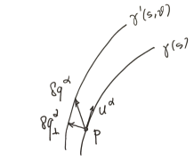
Figure 5: The deviation vector $\delta q^{\alpha}(s)$ connects points of the curve $\gamma(s)$ to the corresponding points of some neighbouring curve $\gamma^{\prime}(s)$. It describes the behaviour of the curves in an infinitesimal neighbourhood of a given curve $\gamma(s)$. The Jacobi equation (3) defines the relative acceleration, i.e. the second order time derivative of the separation $\delta q^{\alpha}(s)$, of two infinitesimally neighbouring curves. The neighbouring curves are arbitrary and not necessary the geodesics. A separation vector $\delta q^{\alpha}$ can be decomposed into the transversal $\delta q^{\alpha}_{\perp}$ and the longitudinal $\delta q^{\alpha}_{\parallel}\propto u^{\alpha}$ components (4.28).

For the second derivative of the deviation vector that defines the relative acceleration the effective tidal force we will get the following expression:

$${D\delta u^{\alpha}\over ds}={D^{2}\delta q^{\alpha}\over ds^{2}}={D\over ds}({D\delta q^{\alpha}\over ds})={D\over ds}(u^{\alpha}_{~{};\beta}\delta q^{\beta})=u^{\alpha}_{~{};\beta;\gamma}u^{\gamma}\delta q^{\beta}+u^{\alpha}_{~{};\beta}~{}{D\delta q^{\beta}\over ds}=$$

$$=-R^{\alpha}_{\beta\gamma\sigma}u^{\beta}\delta q^{\gamma}u^{\sigma}+u^{\alpha}_{~{};\gamma;\beta}u^{\gamma}\delta q^{\beta}+u^{\alpha}_{~{};\beta}u^{\beta}_{~{};\gamma}\delta q^{\gamma}=-R^{\alpha}_{\beta\gamma\sigma}u^{\beta}\delta q^{\gamma}u^{\sigma}+(u^{\alpha}_{~{};\gamma}u^{\gamma})_{;\beta}\delta q^{\beta}.$$ (3.24)

The Jacobi equations, or equations of geodesic deviation, therefore are:

$${D\delta q^{\alpha}\over ds} = u^{\alpha}_{~{};\beta}\delta q^{\beta},$$

$${D^{2}\delta q^{\alpha}\over ds^{2}} = -R^{\alpha}_{\beta\gamma\sigma}u^{\beta}\delta q^{\gamma}u^{\sigma}+(u^{\alpha}_{~{};\gamma}u^{\gamma})_{;\beta}\delta q^{\beta}.$$ (3.25)

There is no requirement for the motion along the curve $\gamma(s)$ to be geodesic. If the curve $\gamma(s)$ is a solution of the geodesic equation (3.18), then the last term in the equation (3) vanishes on the geodesic trajectory $u^{\alpha}_{~{};\gamma}u^{\gamma}=0$ , and the expression for the relative acceleration (3) will simplify and will depend only on the Riemann curvature:

$${D\delta q^{\alpha}\over ds}=u^{\alpha}_{~{};\beta}\delta q^{\beta},~{}~{}~{}~{}~{}~{}~{}{D^{2}\delta q^{\alpha}\over ds^{2}}=-R^{\alpha}_{\beta\gamma\sigma}u^{\beta}\delta q^{\gamma}u^{\sigma}.$$ (3.26)

The vector field $\delta q^{\alpha}$ defined along the geodesic $\gamma(s)$ and satisfying the above equations is called a Jacobi field. The equation can be written also in an alternative first-order form:

$${D\delta q^{\alpha}\over ds}=\delta u^{\alpha},~{}~{}~{}~{}~{}~{}~{}{D\delta u^{\alpha}\over ds}=-R^{\alpha}_{\beta\gamma\sigma}u^{\beta}\delta q^{\gamma}u^{\sigma}.$$ (3.27)

The above form of the Jacobi equations is inconvenient to integrate because they are written in terms of covariant derivatives and, secondly, because they are written in terms of separation of points on geodesic trajectories instead of the physical distance between neighbouring geodesic trajectories. In the next section we will derive the Jacobi equations in terms of physical distance between neighbouring geodesic trajectories and in terms of ordinary proper time derivatives.

4 Jacobi Equations for Transversal Deviations

It is the distance between two neighbouring curves that is of a physical interest, and not the separation of particular points on the neighbouring curves. The aim is to derive the evolution equations for the deviation $\delta q^{\alpha}$ that is perpendicular to the tangent velocity vector $u^{\alpha}$ and lies in the transversal hypersurface $\Sigma_{\perp}$ that is defined by the vector $\delta q^{\alpha}_{\perp}$ normal to the velocity $u_{\alpha}\delta q^{\alpha}_{\perp}=0$. The properties of the transversal deviation vector $\delta q^{\alpha}_{\perp}$ are (see Fig.4 and Fig.5)

$$\delta q^{\alpha}_{\perp}=\delta q^{\alpha}-u^{\alpha}u_{\beta}\delta q^{\beta}=P^{\alpha}_{~{}\beta}\delta q^{\beta},~{}~{}~{}~{}u_{\alpha}\delta q^{\alpha}_{\perp}=0,$$ (4.28)

where the projection operator is

$$P^{\alpha}_{~{}\beta}=\delta^{\alpha}_{\beta}-u^{\alpha}u_{\beta},~{}~{}~{}~{}P^{\alpha}_{~{}\beta}P^{\beta}_{~{}\gamma}=P^{\alpha}_{~{}\gamma},~{}~{}~{}~{}P^{\alpha}_{~{}\beta}u^{\beta}=0,~{}~{}~{}~{}g^{\alpha\beta}P_{\alpha\beta}=3N-1.$$ (4.29)

One can derive the equations for the $\delta q^{\alpha}_{\perp}$ by using the first equation in (3):

$${D\delta q^{\alpha}_{\perp}\over ds}={D(\delta q^{\alpha}-u^{\alpha}u_{\beta}\delta q^{\beta})\over ds}=u^{\alpha}_{~{};\beta}\delta q^{\beta}-u^{\alpha}_{~{};\gamma}u^{\gamma}u_{\beta}\delta q^{\beta}-u^{\alpha}u_{\beta;\gamma}u^{\gamma}\delta q^{\beta}-u^{\alpha}u_{\beta}u^{\beta}_{~{};\gamma}\delta q^{\gamma}=~{}~{}~{}~{}~{}$$

$$=u^{\alpha}_{~{};\beta}P^{\beta}_{~{}\gamma}\delta q^{\gamma}-u^{\alpha}u_{\beta;\gamma}u^{\gamma}\delta q^{\beta}$$ (4.30)

and then project them into the transversal hypersurface $\Sigma_{\perp}$ by using the operator $P^{\alpha}_{~{}\beta}$. Thus we will get

$$P^{\alpha}_{~{}\beta}{D\delta q^{\beta}_{\perp}\over ds}=u^{\alpha}_{~{};\beta}\delta q^{\beta}_{\perp}.$$ (4.31)

For the second derivative one can find

$$P^{\alpha}_{~{}\beta}{D\over ds}(P^{\beta}_{~{}\gamma}{D\delta q^{\gamma}_{\perp}\over ds})=P^{\alpha}_{~{}\beta}{D\over ds}(u^{\beta}_{~{};\gamma}\delta q^{\gamma}_{\perp})=P^{\alpha}_{~{}\beta}(u^{\beta}_{~{};\gamma;\sigma}u^{\sigma}\delta q^{\gamma}_{\perp}+u^{\beta}_{~{};\gamma}~{}u^{\gamma}_{~{};\sigma}\delta q^{\sigma}_{\perp}-u^{\beta}_{~{};\gamma}~{}u^{\gamma}\dot{u}_{\sigma}\delta q^{\sigma}_{\perp})=$$

$$=-R^{\alpha}_{\beta\gamma\sigma}u^{\beta}\delta q^{\gamma}_{\perp}u^{\sigma}+P^{\alpha}_{~{}\beta}(u^{\beta}_{~{};\sigma;\gamma}u^{\sigma}\delta q^{\gamma}_{\perp}+u^{\beta}_{~{};\gamma}~{}u^{\gamma}_{~{};\sigma}\delta q^{\sigma}_{\perp})-P^{\alpha}_{~{}\beta}\dot{u}^{\beta}\dot{u}_{\sigma}\delta q^{\sigma}_{\perp}=$$

$$=-R^{\alpha}_{\beta\gamma\sigma}u^{\beta}\delta q^{\gamma}_{\perp}u^{\sigma}+P^{\alpha}_{~{}\beta}\dot{u}^{\beta}_{~{};\gamma}\delta q^{\gamma}_{\perp}-\dot{u}^{\alpha}\dot{u}_{\beta}\delta q^{\beta}_{\perp},$$ (4.32)

where $\dot{u}^{\alpha}\equiv u^{\alpha}_{~{};\beta}u^{\beta}$ (3.15) is acceleration and $\dot{u}^{\beta}_{~{};\gamma}\equiv(u^{\beta}_{~{};\lambda}u^{\lambda})_{;\gamma}$. Thus the off-shell equations for the first and second derivatives of the transversal deviation are:

$$P^{\alpha}_{~{}\beta}{D\delta q^{\beta}_{\perp}\over ds} = u^{\alpha}_{~{};\beta}\delta q^{\beta}_{\perp},$$

$$P^{\alpha}_{~{}\beta}{D\over ds}(P^{\beta}_{~{}\gamma}{D\delta q^{\gamma}_{\perp}\over ds}) = -R^{\alpha}_{\beta\gamma\sigma}u^{\beta}\delta q^{\gamma}_{\perp}u^{\sigma}+P^{\alpha}_{~{}\beta}\dot{u}^{\beta}_{~{};\gamma}\delta q^{\gamma}_{\perp}-\dot{u}^{\alpha}\dot{u}_{\beta}\delta q^{\beta}_{\perp}.$$ (4.33)

If the curve $\gamma(s)$ fulfils the geodesic equation (3.18), then the relative acceleration depends only on the Riemann curvature:

$$P^{\alpha}_{~{}\beta}{D\delta q^{\beta}_{\perp}\over ds}=u^{\alpha}_{~{};\beta}\delta q^{\beta}_{\perp}~{}~{},$$

$$P^{\alpha}_{~{}\beta}{D\over ds}(P^{\beta}_{~{}\gamma}{D\delta q^{\gamma}_{\perp}\over ds})=-R^{\alpha}_{\beta\gamma\sigma}u^{\beta}\delta q^{\gamma}_{\perp}u^{\sigma}.$$ (4.34)

The system of equations (4) and (4) is written in terms of covariant derivatives, and our aim is to derive these equations in terms of ordinary derivatives. This can be achieved by using the concept of a moving frame [66, 67].

5 Jacobi Equations in Moving Frame

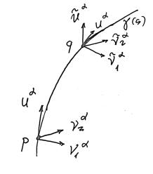
Figure 6: The orthonormal frame $\{u,\nu_{i}\}$ defined in the point $p$ on the curve $\gamma(s)$ parallelly transported into the point $q$. At the point $q$ the frame $\{\tilde{u},\tilde{\nu}_{i}\}$ remains orthonormal but is not anymore orthogonal to the tangential velocity vector $u^{\alpha}$ at $q$. One can construct the orthonormal frame $\{u,\nu_{i}\}$ at each point on the curve $\gamma(s)$ by using the Fermi derivative (5.37).

Let us consider the unit normal vectors $\{\nu^{\alpha}_{i}\}$ that lie in the transversal hypersurface $\Sigma_{\perp}$ (see Fig.4) at some point $\gamma(0)$ on a curve $\gamma(s)$, so that

$$u_{\alpha}\nu^{\alpha}_{i}=0,~{}~{}~{}~{}\nu^{\alpha}_{i}\nu_{j\alpha}=\delta_{ij}~{}~{}~{}~{}~{}at~{}~{}~{}s=0,$$ (5.35)

where $i,j=1,...,3N-1$. One would like to make a parallel transport of the orthonormal frame $\{u,\nu_{i}\}$ along the curve $\gamma(s)$ in order to obtain a similar basis at each point on the curve $\gamma(s)$ (see Fig.6). When the frame vectors (5.35) are parallelly transported along the curve $\gamma(s)$, their covariant derivatives vanish:

$${D\nu^{\alpha}_{i}\over ds}=0,$$ (5.36)

so that the normal vectors will remain orthonormal along the curve $\gamma(s)$ since

$${d\over ds}(\nu^{\alpha}_{i}\nu_{j\alpha})=2\nu^{\alpha}_{i}{D\nu_{\alpha j}\over ds}=0,~{}$$

but they will not remain orthogonal to $u^{\alpha}$ because

$${d\over ds}(u_{\alpha}\nu^{\alpha}_{i})={Du_{\alpha}\over ds}\nu^{\alpha}_{i}+u_{\alpha}{D\nu^{\alpha}_{i}\over ds}={Du_{\alpha}\over ds}\nu^{\alpha}_{i}\neq 0.$$

Geometrically this means that the frame $\{\nu^{\alpha}_{i}\}$ is rotating during a parallel transport along the curve $\gamma(s)$, and the normal frame vectors $\{\nu^{\alpha}_{i}\}$ are not any more orthogonal to the velocity vector $u^{\alpha}$. In order to transport the orthonormal frame $\{u,\nu_{i}\}$ along the curve $\gamma(s)$ without rotation one should use the Fermi derivative [66, 67]

$${D_{F}w^{\alpha}\over ds}={Dw^{\alpha}\over ds}+u^{\alpha}w_{\beta}{Du^{\beta}\over ds}-{Du^{\alpha}\over ds}w_{\beta}u^{\beta}$$ (5.37)

and define the corresponding parallel transport of the normal frame $\{\nu^{\alpha}_{i}\}$ so that now the Fermi derivative of each frame vector vanishes along the curve $\gamma(s)$:

$${D_{F}\nu^{\alpha}_{i}\over ds}=0.$$ (5.38)

In that case one can obtain an orthonormal frame $\{u,\nu_{i}\}$ at each point on the curve $\gamma(s)$ because the Fermi derivative of the velocity vector now vanishes:

$${D_{F}u^{\alpha}\over ds}={Du^{\alpha}\over ds}+u^{\alpha}u_{\beta}{Du^{\beta}\over ds}-{Du^{\alpha}\over ds}u_{\beta}u^{\beta}=0$$ (5.39)

due to the equations (2.9) $u_{\beta}u^{\beta}=1$ and $u_{\beta}{Du^{\beta}\over ds}=0$. Since the covariant derivative preserves the scalar products between parallelly propagated vectors (5.38) and (5.39), the orthogonality relations (5.35) now remain valid along the curve $\gamma(s)$. Thus we have a non-rotating orthonormal frame $\{u,\nu_{i}\}$ along the curve $\gamma(s)$. From the equations (5.37), (5.38) it follows that

$${D_{F}\nu^{\alpha}_{i}\over ds}={D\nu^{\alpha}_{i}\over ds}+u^{\alpha}\nu^{\beta}_{i}{Du_{\beta}\over ds}-{Du^{\alpha}\over ds}\nu^{\beta}_{i}u_{\beta}={D\nu^{\alpha}_{i}\over ds}-u^{\alpha}u_{\beta}{D\nu^{\beta}_{i}\over ds}=P^{\alpha}_{~{}\beta}{D\nu^{\beta}_{i}\over ds}=0$$ (5.40)

and the covariant derivatives of the frame vectors ${D\nu^{\alpha}_{i}\over ds}$ are parallel to the velocity vector $u^{\alpha}$:

$${D\nu^{\alpha}_{i}\over ds}=u^{\alpha}\Big{(}u_{\beta}{D\nu^{\beta}_{i}\over ds}\Big{)}.$$ (5.41)

Now let us consider the equations for the case when the curve $\gamma(s)$ is a geodesic trajectory (3.18). In that case the Fermi derivative (5.37) coincides with the standard covariant derivative:

$${D_{F}w^{\alpha}\over ds}\equiv{Dw^{\alpha}\over ds}.$$ (5.42)

Therefore at each point on the geodesic trajectory $\gamma(s)$ we will have the orthonormal frame $\{u^{\beta},\nu^{\alpha}_{i}\}$ that can be considered as a coordinate system on the tangent vector bundle ${\cal T}^{2(6N-1)}$ projected into the $\gamma(s)$. Let us expand the transversal deviation $\delta q^{\alpha}_{\perp}$ in this basis:

$$\delta q^{\alpha}_{\perp}=\sum^{3N-1}_{i=1}\rho_{i}~{}\nu^{\alpha}_{i}~{},$$ (5.43)

where along the whole geodesic trajectory $\gamma(s)$ we have now the orthonormal frame $\{u^{\beta},\nu^{\alpha}_{i}\}$:

$$u_{\alpha}\nu^{\alpha}_{i}=0,~{}~{}~{}~{}\nu^{\alpha}_{i}\nu_{j\alpha}=\delta_{ij},~{}~{}~{}~{}g^{\alpha\beta}=\sum_{i}\nu^{\alpha}_{i}\nu^{\beta}_{i}+u^{\alpha}u^{\beta}.$$ (5.44)

The system of equations (4) for transversal deviation written in terms of covariant derivatives now can be written in terms of ordinary derivatives. The covariant derivative of (5.43) is

$$P^{\alpha}_{~{}\beta}{D\delta q^{\beta}_{\perp}\over ds}=\dot{\rho}_{i}~{}\nu^{\alpha}_{i}+\rho_{i}~{}P^{\alpha}_{~{}\beta}{D\nu^{\beta}_{i}\over ds}=\dot{\rho}_{i}~{}\nu^{\alpha}_{i}$$ (5.45)

where $P^{\alpha}_{~{}\beta}\nu^{\beta}_{i}=\nu^{\alpha}_{i}$, ${D\nu^{\alpha}_{i}\over ds}=0$ due to (5.42) and (5.38) and $\dot{\rho}_{i}\equiv{d\rho_{i}\over ds}$. The projection of the above equation to the transversal hypersurface $\Sigma_{\perp}$ is

$$\nu_{i\alpha}P^{\alpha}_{~{}\beta}{D\delta q^{\beta}_{\perp}\over ds}=\dot{\rho}_{i}.$$ (5.46)

The first Jacobi equation (4) will take the following form:

$$\dot{\rho}_{i}=\sum_{j}(\nu^{\alpha}_{i}u_{\alpha;\beta}\nu^{\beta}_{j})~{}\rho_{j}=u_{ij}~{}\rho_{j},$$ (5.47)

where

$$u_{ij}=\nu^{\alpha}_{i}u_{\alpha;\beta}\nu^{\beta}_{j}.$$ (5.48)

For the second derivative in (4) we will get

$$P^{\alpha}_{~{}\beta}{D\over ds}(P^{\beta}_{~{}\gamma}{D\delta q^{\gamma}_{\perp}\over ds})=P^{\alpha}_{~{}\beta}{D\over ds}(\dot{\rho}_{j}~{}\nu^{\beta}_{j})=P^{\alpha}_{~{}\beta}\Big{(}\ddot{\rho}_{j}~{}\nu^{\beta}_{j}+\dot{\rho}_{j}~{}{D\nu^{\beta}_{j}\over ds}\Big{)}=\ddot{\rho}_{j}~{}P^{\alpha}_{~{}\beta}\nu^{\beta}_{j}=\ddot{\rho}_{j}~{}\nu^{\alpha}_{j}~{},$$ (5.49)

therefore the second equation (4) will take the following form:

$$\ddot{\rho}_{i}=-R_{\alpha\beta\gamma\sigma}\nu^{\alpha}_{i}u^{\beta}\nu^{\gamma}_{j}u^{\sigma}\rho_{j}.$$ (5.50)

In summary, the Jacobi deviation equations on the geodesic trajectories (5.47) and (5.50) are

$$\dot{\rho}_{i}=u_{ij}~{}\rho_{j},~{}~{}~{}~{}~{}~{}~{}\ddot{\rho}_{i}=-R_{ij}\rho_{j},~{}~{}~{}~{}~{}~{}~{}i,j=1,...,3N-1~{},$$ (5.51)

where

$$R_{ij}=R_{\alpha\beta\gamma\sigma}\nu^{\alpha}_{i}u^{\beta}\nu^{\gamma}_{j}u^{\sigma},~{}~{}~{}u_{ij}=\nu^{\alpha}_{i}u_{\alpha;\beta}\nu^{\beta}_{j},~{}~{}~{}~{}\delta q^{\alpha}_{\perp}=\sum^{3N-1}_{i=1}\rho_{i}~{}\nu^{\alpha}_{i}~{}~{}~{}$$ (5.52)

We have a system of ordinary differential equations, and since the differential equations have smooth coefficients, the solutions exist for all $s$, are unique given $\rho_{i}(s_{0})$ and $\dot{\rho}_{i}(s_{0})$ at some point on $\gamma(s)$, and there will be $2(3N-1)$ independent Jacobi fields along $\gamma(s)$. There will be twice less $3N-1$ independent Jacobi fields if initially $\rho_{i}(s_{0})=0$ at some point on $\gamma(s)$ (see Appendix B for details).

Let us introduce the sectional curvature on the two-dimensional tangent plane defined by the two vectors $(u,v)$ as

$$K(q,u,v)={R_{\alpha\beta\gamma\delta}(q)~{}v^{\alpha}u^{\beta}v^{\gamma}u^{\delta}\over|u\wedge v|^{2}},$$ (5.53)

where $|u\wedge v|^{2}=|u|^{2}|v|^{2}-(u\cdot v)^{2}$ and the norm is defined through the scalar product:

$$(u\cdot v)=g_{\alpha\beta}u^{\alpha}v^{\beta},~{}~{}~{}~{}~{}|u|^{2}=(u\cdot u)=g_{\alpha\beta}u^{\alpha}u^{\beta}.$$ (5.54)

The relation between tensor $R_{ij}$ and the sectional curvature (5.53) can be expressed in the following form:

$$K(q,u,\delta q_{\perp})={R_{\alpha\beta\gamma\sigma}\delta q_{\perp}^{\alpha}u^{\beta}\delta q_{\perp}^{\gamma}u^{\sigma}\over|\delta q_{\perp}|^{2}}={\sum_{ij}R_{ij}\rho_{i}\rho_{j}\over\sum_{i}\rho^{2}_{i}}~{},$$ (5.55)

where we used the decomposition (5.43). Having in hand the equations (5.51) for the normal deviation $\delta q_{\perp}$ in terms of ordinary proper time derivatives one can derive the equation for the scalar $|\delta q_{\perp}|^{2}$. The norm $|\delta q_{\perp}|^{2}$ of the transversal deviation can be computed by using (5.43):

$$|\delta q_{\perp}|^{2}=\sum_{i}\rho^{2}_{i},$$ (5.56)

and its derivatives by means of the above equations (5.51):

$${d\over ds}|\delta q_{\perp}|^{2} = 2\rho_{i}\dot{\rho}_{i}=2u_{ij}\rho_{i}\rho_{j}=2\delta q_{\perp}^{\alpha}u_{\alpha;\beta}\delta q_{\perp}^{\beta},$$ (5.57)

$${d^{2}\over ds^{2}}|\delta q_{\perp}|^{2} = 2\rho_{i}\ddot{\rho}_{i}+2\dot{\rho}_{i}\dot{\rho}_{i}=-2R_{ij}\rho_{i}\rho_{j}+2u_{ik}u_{ij}\rho_{k}\rho_{j}=-2R_{\alpha\beta\gamma\lambda}\delta q^{\alpha}_{\perp}u^{\beta}\delta q^{\gamma}_{\perp}u^{\lambda}+2u^{\gamma}_{~{};\alpha}u_{\gamma;\beta}\delta q^{\alpha}_{\perp}\delta q^{\beta}_{\perp}.$$

Thus by using the sectional curvature (5.55) one can obtain on-shell equations for the scalar $|\delta q_{\perp}|^{2}$ in terms of proper time derivatives:

$${d\over ds}|\delta q_{\perp}|^{2} = 2\delta q_{\perp}^{\alpha}u_{\alpha;\beta}\delta q_{\perp}^{\beta}$$

$${d^{2}\over ds^{2}}|\delta q_{\perp}|^{2} = -2K(q,u,\delta q_{\perp})|\delta q_{\perp}|^{2}+2|\delta u_{\perp}|^{2}.$$ (5.58)

The last term is a square of the deviation velocity (3.23) and is positive-definite: $u^{\gamma}_{~{};\alpha}\delta q^{\alpha}_{\perp}u_{\gamma;\beta}\delta q^{\beta}_{\perp}=|\delta u_{\perp}|^{2}\geq 0$. The advantage of this form of the deviation equations is that they are written mostly in terms of ordinary time derivatives, but still the last term is written in terms of a covariant derivative. In Appendix C we suggested an additional estimate for the the last term in the Anosov equation (5) that makes relaxation time (6.69) shorter (3.210).

6 Exponential Instability, Lyapunov exponent and Dynamical Chaos

It follows that in order to study the stability of the trajectories of self-gravitating N-body systems one should know the properties of the sectional curvature that is entering into the Jacobi equations (5). It is our main concern to investigate the sign of the sectional curvature $K(q,u,\delta q_{\perp})$ that defines the stability of geodesic trajectories in different parts of the extended phase space $(q,u,\delta q,\delta u)\in{\cal T}^{2(6N-1)}$. In the regions where the sectional curvature is negative the trajectories are unstable, exponentially diverging and the dynamical system is in a chaotic phase, while in the regions where the sectional curvature is positive the trajectories are stable and can exhibit the geodesic focusing generating the conjugate points and caustics.

Let us consider first the behaviour of a system that has a negative sectional curvature. The following Anosov inequality takes place for the relative acceleration [80]:

$${d^{2}\over ds^{2}}|\delta q_{\perp}|^{2}\geq-2K(q,u,\delta q_{\perp})~{}|\delta q_{\perp}|^{2}$$ (6.59)

and can be integrated in the case when the sectional curvatures are globally negative all over the phase space [80]:

$$K(q,u,\delta q_{\perp})\leq-\kappa<0,$$ (6.60)

where $\kappa=\min|K(q,u,\delta q_{\perp})|_{\{q,u,\delta q_{\perp}\}}>0$. It follows then that

$${d^{2}\over ds^{2}}|\delta q_{\perp}|^{2}\geq 2\kappa~{}|\delta q_{\perp}|^{2}$$ (6.61)

and therefore for all $s$

$${d^{2}\over ds^{2}}|\delta q_{\perp}|^{2}>0,$$ (6.62)

that is, $|\delta q_{\perp}|^{2}$ is a convex function (see also Appendix B). The behaviour of the solutions of the above equation depends on the sign of the first derivative. The solutions that have positive initial first derivative

$${d|\delta q_{\perp}(s)|^{2}\over ds}|_{s=0}>0$$ (6.63)

are describing exponentially expanding geodesic trajectories

$$|\delta q_{\perp}(s)|\geq{1\over 2}|\delta q_{\perp}(0)|e^{\sqrt{2\kappa}s}$$ (6.64)

and the inequality that follows from (3.27) [80],

$$|\delta u(s)|\geq Const.~{}|\delta q_{\perp}(s)|,$$ (6.65)

defines the exponential expansion of the velocity vector $u^{\alpha}(s)$. Similarly, the solutions that have negative initial first derivative,

$${d|\delta q_{\perp}(s)|^{2}\over ds}|_{s=0}<0,$$ (6.66)

are describing exponentially contracting geodesic trajectories

$$|\delta q_{\perp}(s)|\leq{1\over 2}|\delta q_{\perp}(0)|e^{-\sqrt{2\kappa}s}$$ (6.67)

and of the corresponding velocity

$$|\delta u(s)|\leq Const.~{}|\delta q_{\perp}(s)|.$$ (6.68)

In Hamiltonian mechanics the simultaneous coexistence of exponentially expanding and contracting sets of geodesic trajectories is a necessary consequence of the Liouville’s theorem. In the literature it is common to call the index $\sqrt{2\kappa}$ a maximal Lyapunov exponent.

Following Krilov work on relaxation phenomena [85], the exponential instability of the geodesic trajectories defines the characteristic relaxation time [85, 90, 49, 50, 51] (see also (3.210)):

$$\tau={1\over\sqrt{2\kappa}}.$$ (6.69)

We will apply the above result (6.69) to self-gravitating N-body systems in the next section.

The geodesic flow on manifolds of negative sectional curvature defines an important class of dynamical systems advocated by Anosov [80], and they are relevant for the investigation of gauge field theory dynamics [47, 49, 50], the motion of stars in galaxies and globular clusters [51], the fluid-flow stability and turbulence [87, 91] and can be used to produce high quality random numbers for the Monte Carlo simulations [90, 92, 93].

In summary, we have the Jacobi equations (5.51), (5.52) and the equations (5) that describe the deviation of the geodesic trajectories in terms of ordinary proper time derivatives. In order to study the stability of the trajectories of self-gravitating the N-body systems one should know the properties of the sectional curvature $K(q,u,\delta q_{\perp})$ that is entering into the Jacobi equations (5). It is our main concern to investigate the sign of the sectional curvature $K(q,u,\delta q_{\perp})$ that defines the stability of geodesic trajectories in different parts of the phase space. In the regions where the sectional curvature is negative trajectories are unstable, exponentially diverging and the dynamical system is in a chaotic phase, while in areas where the sectional curvature is positive the trajectories are stable and can exhibit the geodesic focusing, conjugate points and caustics. In the next section we will derive useful expressions for the sectional curvatures and will apply the results to the investigation of self-gravitating N-body systems.

7 Collective Relaxation of Self-Gravitating N-body Systems

Let us consider the sectional curvature $K(q,u,\delta q_{\perp})$ and investigate the regions of the phase space where it has a definite sign. The sectional curvature (5.53) in the case of Maupertuis’s metric (2.8) and Riemann curvature tensor (11.162) will take the following form:

$${R_{\alpha\beta\gamma\delta}v^{\alpha}u^{\beta}v^{\gamma}u^{\delta}}= - {3\over 4W^{2}}\Big{(}2(uv)(uW^{{}^{\prime}})(vW^{{}^{\prime}})-|v|^{2}(uW^{{}^{\prime}})^{2}-|u|^{2}(vW^{{}^{\prime}})^{2}\Big{)}-$$ (7.70)

$$- {1\over 4W^{2}}(|u|^{2}|v|^{2}-(uv)^{2})|W^{{}^{\prime}}|^{2}+$$

$$+ {1\over 2W}\Big{(}2(uv)(uW^{{}^{\prime\prime}}v)-|v|^{2}(uW^{{}^{\prime\prime}}u)-|u|^{2}(vW^{{}^{\prime\prime}}v)\Big{)},$$

where

$$(uW^{{}^{\prime}})=u^{\alpha}{\partial W\over\partial q^{\alpha}},~{}~{}(uW^{{}^{\prime\prime}}u)=u^{\alpha}{\partial^{2}W\over\partial q^{\alpha}\partial q^{\beta}}u^{\beta},~{}~{}(vW^{{}^{\prime}})=v^{\alpha}{\partial W\over\partial q^{\alpha}},~{}~{}(uW^{{}^{\prime\prime}}v)=u^{\alpha}{\partial^{2}W\over\partial q^{\alpha}\partial q^{\beta}}v^{\beta},$$

and the Riemann tensor is given in (11.162). By using the general expression (7.70) for the sectional curvature and substituting the vectors $u$ and $v=\delta q_{\perp}$ that are orthogonal to each other $(u\cdot\delta q_{\perp})=0$ (4.28) and because $|u|^{2}=1$ we will get

$${R_{\alpha\beta\gamma\delta}\delta q_{\perp}^{\alpha}u^{\beta}\delta q_{\perp}^{\gamma}u^{\delta}}=-{1\over 4W^{2}}|W^{{}^{\prime}}|^{2}|\delta q_{\perp}|^{2}+{3\over 4W^{2}}\Big{(}(uW^{{}^{\prime}})^{2}|\delta q_{\perp}|^{2}+(\delta q_{\perp}W^{{}^{\prime}})^{2}\Big{)}-$$

$$-{1\over 2W}\Big{(}(uW^{{}^{\prime\prime}}u)|\delta q_{\perp}|^{2}+(\delta q_{\perp}W^{{}^{\prime\prime}}\delta q_{\perp})\Big{)},$$ (7.71)

where the force vector is

$$F_{\alpha}=-{\partial W\over\partial q^{\alpha}}={\partial U\over\partial q^{\alpha}}.$$ (7.72)

We can also calculate the sectional curvature tensor (5.52) by using (7) (see Appendix A):

$$R_{ij}=R_{\alpha\beta\gamma\delta}\nu^{\alpha}_{i}u^{\beta}\nu^{\gamma}_{j}u^{\delta}=-{3\over 4W^{2}}\delta_{ij}\Big{(}{1\over 3}|W^{{}^{\prime}}|^{2}-(uW^{{}^{\prime}})^{2}\Big{)}+{3\over 4W^{2}}(\nu_{i}W^{{}^{\prime}})(\nu_{j}W^{{}^{\prime}})-$$

$$-{1\over 2W}\Big{(}\delta_{ij}(uW^{{}^{\prime\prime}}u)+(\nu_{i}W^{{}^{\prime\prime}}\nu_{j})\Big{)}.$$ (7.73)

The first three terms of the sectional curvature tensors (7) and (7) are proportional to the first order derivatives of the potential function and decrease as a square of the distance between particles $W^{{}^{\prime}}\sim 1/r^{2}_{ab}$, while the last two terms are proportional to the second order derivatives of the potential function and decrease as a cube of the distance between particles $W^{{}^{\prime\prime}}\sim 1/r^{3}_{ab}$ (7.75), (7). If the distribution of particles is almost spherical in space, then the quadrupole moment of the system is close to zero, $\sum D_{ab}\approx 0$, and the second order derivative terms are additionally suppressed by a quadrupole moment (7). In the forthcoming sections we will consider the second derivatives terms as the perturbation that can be safely omitted in the first order approximation. We have to notice that in the general relativity the Riemann curvature tenser contains terms that are also proportional to the first and second order derivatives of the gravitational potential function and it is not accidental that the sectional curvatures here have a similar structure. The physical significance of these terms in the Effective Field Theory of Large Scale Structures (EFTofLSS) was recently discussed in [31, 32, 39, 33, 34, 40, 37, 36, 35].

The self-gravitating system of $N$ particles interacts through the gravitational potential function of the form

$$U=-G\sum_{a<b}{M_{a}M_{b}\over r_{ab}},~{}~{}~{}~{}~{}~{}~{}~{}~{}~{}~{}r^{i}_{ab}=r^{i}_{a}-r^{i}_{b}~{}~{}~{}~{}~{}i=1,2,3~{}~{}~{}~{}~{}~{}~{}a,b=1,...,N~{}~{}~{}~{}$$ (7.74)

and the derivatives of the potential function are

$${\partial U\over\partial q^{\alpha}}\rightarrow{1\over M^{1/2}_{a}}{\partial U\over\partial r^{i}_{a}},~{}~{}~{}~{}~{}{\partial U\over\partial r^{i}_{a}}=\sum_{b,b\neq a}G{M_{a}M_{b}\over r^{3}_{ab}}r^{i}_{ab},~{}~{}~{}{\partial^{2}U\over\partial q^{\alpha}\partial q^{\beta}}\rightarrow{1\over(M_{a}M_{b})^{1/2}}{\partial^{2}U\over\partial r^{i}_{a}\partial r^{j}_{b}},$$ (7.75)

where for the second derivatives one can get

$${\partial^{2}U\over\partial r^{i}_{a}\partial r^{j}_{b}} = G{M_{a}M_{b}\over r^{5}_{ab}}D^{ij}_{ab},~{}~{}~{}~{}b\neq a$$

$${\partial^{2}U\over\partial r^{i}_{a}\partial r^{j}_{a}} = -G\sum_{c,c\neq a}{M_{a}M_{c}\over r^{5}_{ac}}D^{ij}_{ac}+\sum_{c,c\neq a}{4\pi GM_{a}M_{c}\over 3}\delta^{ij}\delta^{(3)}(\vec{r}_{ac}).$$ (7.76)

Here $D^{ij}_{ab}=3r^{i}_{ab}r^{j}_{ab}-\delta^{ij}r^{2}_{ab}$ is a quadrupole moment, and the trace of the second order derivatives is equal to the Laplacian of the potential function

$$\sum_{a,i}{\partial^{2}U\over\partial r^{i}_{a}\partial r^{i}_{a}}=4\pi G\sum_{a\neq c}M_{a}M_{c}~{}\delta^{(3)}(\vec{r}_{ac})$$ (7.77)

and differs from zero only in the cases of direct collision of the particles $\vec{r}_{ab}=0$.

By introducing angles between force vector $F_{\alpha}={\partial W\over\partial q^{\alpha}}$ and vectors $u^{\alpha}$ and $\delta q^{\alpha}_{\perp}$ we can express the scalar products in term of corresponding angles:

$$(u\cdot W^{{}^{\prime}})=|W^{{}^{\prime}}|\cos\theta_{u},~{}~{}~{}~{}~{}(\delta q_{\perp}\cdot W^{{}^{\prime}})=|W^{{}^{\prime}}||\delta q_{\perp}|\cos\theta_{\delta q_{\perp}},$$ (7.78)

where $\theta_{u}$ is the angle between the $F^{\alpha}$ (7.72) and velocity $u^{\alpha}$, while the $\theta_{\delta q_{\perp}}$ is the angle between $F^{\alpha}$ and deviation vector $\delta q^{\alpha}_{\perp}$. For the $\cos^{2}\theta_{u}$ we obtained the following expression:

$$\cos^{2}\theta_{u}={\Big{(}\sum_{a}\dot{\vec{r}}_{a}{\partial U\over\partial\vec{r}_{a}}\Big{)}^{2}\over\Big{(}\sum_{a}M_{a}\dot{\vec{r}}_{a}\dot{\vec{r}}_{a}\Big{)}\Big{(}\sum_{a}{1\over M_{a}}{\partial U\over\partial\vec{r}_{a}}{\partial U\over\partial\vec{r}_{a}}\Big{)}}={\Big{(}\sum_{a}M_{a}\dot{\vec{r}}_{a}\ddot{\vec{r}}_{a}\Big{)}^{2}\over\Big{(}\sum_{a}M_{a}\dot{\vec{r}}_{a}\dot{\vec{r}}_{a}\Big{)}\Big{(}\sum_{a}M_{a}\ddot{\vec{r}}_{a}\ddot{\vec{r}}_{a}\Big{)}}.$$ (7.79)

The contracted Riemann tensor in (5.55) and (7) reduces to the expression

$$R_{\alpha\beta\gamma\delta}\delta q^{\alpha}_{\perp}u^{\beta}\delta q^{\gamma}_{\perp}u^{\delta} = K(q,u,\delta q_{\perp})~{}|\delta q_{\perp}|^{2}={3\over 4W^{2}}\Big{(}\cos^{2}\theta_{u}+\cos^{2}\theta_{\delta q_{\perp}}-{1\over 3}\Big{)}|W^{{}^{\prime}}|^{2}|\delta q_{\perp}|^{2},~{}~{}~{}~{}~{}~{}$$ (7.80)

and the sectional curvature (5.55) will take the following form (see Fig.7):

$$K(q,u,\delta q_{\perp})={3|W^{{}^{\prime}}|^{2}\over 4W^{2}}\Big{(}\cos^{2}\theta_{u}+\cos^{2}\theta_{\delta q_{\perp}}-{1\over 3}\Big{)}.$$ (7.81)

This form of the sectional curvature is convenient to analyse and locate the regions where the sectional curvature has a definite sign.

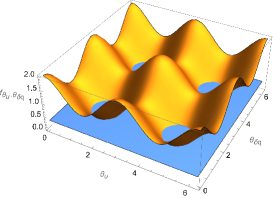
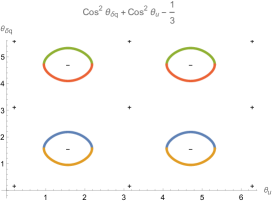
Figure 7: The left figure shows the surfaces $f(\theta_{u},\theta_{\delta q})=\cos^{2}\theta_{u}+\cos^{2}\theta_{\delta q}$ and $f={1\over 3}$. The sectional curvature (7.81) is positive above the horizontal surface $f={1\over 3}$ and is negative below the horizontal surface. The right figure shows the curve $\cos^{2}\theta_{u}+\cos^{2}\theta_{\delta q}-{1\over 3}=0$. Inside the four circles the sectional curvature is negative, and outside it is positive. The maximum and minimum values of the sectional curvature are marked.

Indeed, during the evolution of an N-body system the sectional curvatures can be either positive or negative depending of the sign of the expression

$$\cos^{2}\theta_{u}+\cos^{2}\theta_{\delta q_{\perp}}-{1\over 3},$$ (7.82)

and it allows to find the maximal and minimal values of the sectional curvature (see Fig.7):

$$K(u,\delta q_{\perp})|_{max}=+{5\over 4W^{2}}|W^{{}^{\prime}}|^{2},~{}~{}~{}~{}~{}K(u,\delta q_{\perp})|_{min}=-{1\over 4W^{2}}|W^{{}^{\prime}}|^{2}.$$ (7.83)

For the tensor $R_{ij}$ (7) in the same approximation we will get (see Appendix A)

$$R_{ij} = {3\over 4W^{2}}\Big{(}\delta_{ij}\Big{(}(u\cdot W^{{}^{\prime}})^{2}-{1\over 3}|W^{{}^{\prime}}|^{2}\Big{)}+(\nu_{i}W^{{}^{\prime}})(\nu_{j}W^{{}^{\prime}})\Big{)}=$$ (7.84)

$$= {3|W^{{}^{\prime}}|^{2}\over 4W^{2}}\Big{(}\delta_{ij}(\cos^{2}\theta_{u}-{1\over 3})+\cos\theta_{i}\cos\theta_{j}\Big{)},$$

where $(\nu_{i}W^{{}^{\prime}})=|W^{{}^{\prime}}|\cos\theta_{i}$ and

$$\cos^{2}\theta_{i}={\Big{(}\sum_{a}{1\over M^{1/2}_{a}}\vec{\nu}^{(i)}_{a}{\partial U\over\partial\vec{r}_{a}}\Big{)}^{2}\over\Big{(}\sum_{a}{1\over M_{a}}{\partial U\over\partial\vec{r}_{a}}{\partial U\over\partial\vec{r}_{a}}\Big{)}}={\Big{(}\sum_{a}M^{1/2}_{a}\vec{\nu}^{(i)}_{a}\ddot{\vec{r}}_{a}\Big{)}^{2}\over\Big{(}\sum_{b}M_{a}\ddot{\vec{r}}_{a}\ddot{\vec{r}}_{a}\Big{)}}.$$ (7.85)

If the initial distribution of velocities $u^{\alpha}$ is without any noticeable symmetry, $\cos\theta_{u}\sim 0$, the perturbations are in arbitrary directions $\cos\theta_{\delta q_{\perp}}\sim 0$ and the system has a small quadrupole moment, then the system is located in the phase space region of the negative sectional curvatures (7.83) and we can estimate the shortest relaxation time $\tau_{short}$ of an almost spherically symmetric N-body system. In accordance with the expressions (6.64) and (6.67) the instability has an exponential character and the relaxation time is defined as in (6.69):

$${1\over\sqrt{2\kappa}}={1\over\sqrt{2|K(u,\delta q_{\perp})_{min}|}}=\sqrt{{2W^{2}\over|W^{{}^{\prime}}|^{2}}}=\sqrt{{2W^{3}\over(\nabla W)^{2}}}.$$ (7.86)

Converting the proper time $s$ into the physical time $t$, which was defined in (2.12), we will obtain for the shortest relaxation time the expression

$$\tau_{collective}=\sqrt{{W\over(\nabla W)^{2}}},$$ (7.87)

where $W$ is the total kinetic energy of an N-body system and $(\nabla W)^{2}$ is a square of the gravitational force acting on a unit mass of a particle (7.72), (7.75). It is the shortest relaxation time scale since it is realised when the sectional curvature has its minimal value (7.83) (see Fig.7). Considering the behaviour of stars in the elliptic galaxies one can get

$$W=T=\sum^{N}_{a=1}\Big{(}{M_{a}v^{2}_{a}\over 2}\Big{)}\simeq N{M\langle v^{2}\rangle\over 2},~{}~{}~{}~{}~{}~{}(\nabla W)^{2}=\sum^{N}_{a=1}{1\over M_{a}}\Big{(}{\partial U\over\partial\vec{r}_{a}}\Big{)}^{2}=\sum^{N}_{a=1}\varepsilon^{2}_{a}\simeq N\langle\varepsilon\rangle^{2},$$ (7.88)

where the Holtsmark mean square force [94, 41] is $\langle\varepsilon\rangle^{2}=a^{4/3}M$, $a={4\over 15}(2\pi GM)^{3/2}n$, $n$ is the mean stellar density and $M$ is the mean star mass. Each term in the last sum can be approximated by the force ${GM\over d^{2}}$ acting on a star by a nearby star at a distance $d$, where $d$ is the mean distance between stars. For the shortest collective relaxation time we will get

$$\tau_{collective}=\sqrt{{W\over(\nabla W)^{2}}}=\gamma{\langle v^{2}\rangle^{1/2}\over\pi GMn^{2/3}},$$ (7.89)

where the numerical coefficient $\gamma=(15/4)^{2/3}1/2\sqrt{2}$. Comparing the collective relaxation time (7.89) with the Smart-Ambarsumian-Chandrasekhar-Spitzer relaxation time $\tau_{b}$, which is due to the binary encounters of stars [95, 70, 71, 96, 94, 51, 43, 42, 41], one can get

$${\tau_{b}\over\tau_{collective}}={\langle v^{2}\rangle^{3/2}\over G^{2}M^{2}n\log N}{2GMn^{2/3}\over\langle v^{2}\rangle^{1/2}}={\langle v^{2}\rangle\over GMn^{1/3}}{2\over\log N}~{}\propto~{}{d\over r_{*}}$$ (7.90)

where $r_{*}={2GM\over\langle v^{2}\rangle}$ is the radius of effective binary scattering of stars. As the astrophysical observations revealed $d\gg r_{*}$, we will get that the collective relaxation time $\tau_{collective}$ is much shorter than the binary relaxation time $\tau_{collective}\ll\tau_{b}$. These time scales and the dynamical time scale (crossing time)

$$\tau_{dyn}={D\over\langle v^{2}\rangle^{1/2}}={D^{3/2}\over(GNM)^{1/2}},$$ (7.91)

which is the time interval for a star to cross a gravitating system of a characteristic size $D$, are in the following relation:

$$\tau_{collective}\approx{D\over d}\tau_{dyn},~{}~{}~{}~{}\tau_{b}\approx{D\over r_{*}}\tau_{dyn}.$$ (7.92)

These relations demonstrate the hierarchies of the time scales and the length scales that naturally appear in the self-gravitating system in equilibrium :

$$\tau_{dyn}<\tau_{collective}<\tau_{b}$$

$$D~{}~{}~{}>~{}~{}~{}d>~{}~{}~{}~{}r^{*}.$$ (7.93)

The collective relaxation time (7.89) for typical elliptical galaxies is of the following order [51]:

$$\tau_{galaxies}\simeq 6.14\times 10^{9}\Big{(}{\langle v^{2}\rangle^{1/2}\over 100{km\over s}}\Big{)}\Big{(}{1pc^{-3}\over n}\Big{)}^{2/3}\Big{(}{M_{\odot}\over M}\Big{)}~{}years.$$ (7.94)

This time is by few orders of magnitude shorter than the binary relaxation time.

Elliptical galaxies tend to have higher stellar densities in their central part compared to their outer regions. This concentration of stars creates a dense core known as a galactic bulge. The density of stars in a core of elliptical galaxies and globular clusters can be as large as a few million stars per cubic parsec, therefore the absolute value of the negative sectional curvatures and the corresponding exponential divergency will be larger and the relaxation time even shorter. The Hubble Deep Field and Hubble eXtreme Deep Field images revealed a large number of distant young galaxies seemingly in a non-equilibrium state, while the stars in the nearby older galaxies show a more regular distribution of velocities and shapes, reflecting the collective relaxation mechanism of stars.

Let us also estimate the collective relaxation time for a typical galactic cluster. The three-dimensional velocity dispersion inside a gravitationally bound cluster of galaxies is typically $\langle v^{2}\rangle^{1/2}\approx 1000km/s$ [13]. The dynamical time scale $t_{dyn}$ is equal to the cluster crossing time:

$$t_{dyn}\approx{D\over\langle v^{2}\rangle^{1/2}}=10^{9}\Big{(}{D\over Mpc}\Big{)}\Big{(}{1000kms^{-1}\over\langle v^{2}\rangle^{1/2}}\Big{)}~{}years.$$ (7.95)

In the case of Coma cluster for the collective relaxation time scale (7.89) we will get

$$\tau_{claster}\approx 10^{11}\Big{(}{\langle v^{2}\rangle^{1/2}\over 1000{km\over s}}\Big{)}\Big{(}{8.7Mpc^{-3}\over n_{g}}\Big{)}^{2/3}\Big{(}{M_{c}\over M}\Big{)}~{}years,$$ (7.96)

where the formula is normalised to the Coma cluster mass $M_{c}\approx 7\times 10^{14}M_{\odot}$, to the mean galactic density $n_{g}$ in the Coma cluster of 1000 galaxies inside the sphere of the diameter of $6.13$ Mpc and the average galaxy mass of order $M_{g}=10^{11}M_{\odot}$ (for the Coma cluster $r_{*}=1.3\times 10^{21}cm$ and $d=1.9\times 10^{24}cm$, in agreement with (7.92)). As it should be (see 7), the collective relaxation time is larger than the dynamical time scale (crossing time) (see also Appendix F).

8 Geodesic Focusing and Caustics of Self-Gravitating N-body Systems

Let us now consider the physical conditions at which a self-gravitating system is developing a geodesic focusing and caustics. In the case of a radial expansion or contraction, when the force and velocity are almost collinear, $\cos^{2}\theta_{u}\simeq 1$ in (7.78), and the perturbation $\delta q_{\perp}$ is normal or is collinear to the force (the angular $\theta_{\delta q_{\perp}}$ is in the interval $0\leq\theta_{\delta q_{\perp}}\leq 90^{o}$, that is, $0\leq\cos\theta_{\delta q_{\perp}}\leq 1$), the sectional curvature (7.81) is positive and the system will develop geodesic focusing, the conjugate points and caustics.

The caustics are regions of the coordinate space where the density of particles is higher than the average particle density. We can estimate the time scale at which the radially expanding or contracting self-gravitating system of particles/galaxies will evolve and contract into the higher-density caustics, the regions where they will pile up into low-dimensional hyper-surfaces and filaments.

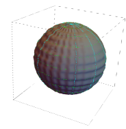
Figure 8: A dark spherical region represents the initial density perturbation surrounded by the uniformly expanding Universe. It was assumed by Gunn and Gott [76] that at the epoch of recombination, when the redshift is about $1+z_{i}\approx 1100$, there exist spherical regions that have density slightly higher than the density of the surrounding Universe. If $\rho_{ci}$ was the critical density at this epoch, $\rho_{ci}=3H^{2}_{i}/8\pi G$, where $H_{i}$ is the Hubble parameter appropriate to the epoch $z_{i}$, then for densities in excess of $\rho_{ci}$ of the form $\rho_{ci}+\delta\rho_{i}$, where $\delta\rho_{i}$ represents the perturbation, the particles will expand to a maximum radius and then collapse again generating the density contrast $\delta\rho/\rho$ (8.111), (8.112) at the Hubble time scale (8.115). In this model the galaxies and clusters of galaxies develop from the small-density perturbations that survived until the recombination time.

Thus the positivity of sectional curvature (7.81) has an effect of prime importance: Once the geodesics of the congruence $\{\gamma\}$ start to converge, then they must, within a finite interval of proper time, inevitably contract to a caustic. We can estimate the characteristic time scale of the appearance of caustics by using the maximum positive value of the sectional curvatures (7.83):

$${1\over\sqrt{2K(u,\delta q_{\perp})_{max}}}=\sqrt{{2W^{2}\over 5|W^{{}^{\prime}}|^{2}}}=\sqrt{{2W^{3}\over 5(\nabla W)^{2}}},$$ (8.97)

thus the characteristic time scale of the appearance of caustics is

$$\tau_{caustics}={1\over 3}\sqrt{{W\over 5(\nabla W)^{2}}}.$$ (8.98)

The above kinematics very well fits with the kinematics of the expanding Universe because here the radial gravitational force and velocity are collinear, $\cos^{2}\theta_{u}\simeq 1$, and the sectional curvatures are positive. Thus we have to estimate the quantities $W$ and $(\nabla W)^{2}$ in the above equation.

Let us consider the evolution of a spherical shell of radius $R_{0}$ that expands with the Universe, so that $R=R_{0}~{}a(t)$ and $a(t)$ is the scale factor in the Newtonian cosmological model of the expanding Universe [97, 98, 14, 19, 24] (see Appendix II in [24]). One can derive the evolution of $a(t)$ by using mostly the Newtonian mechanics and accepting two results from the general relativity: The Birkhoff’s theorem stated that for a spherically symmetric system the force due to gravity at radius $R$ is determined only by the mass interior to that radius and that the energy contributes to the gravitating mass density through the matter density $\rho_{m}$ at zero pressure, $p=0$, and the energy density of radiation/relativistic particles, $\rho_{r}=3p/c^{2}$, where $p=\epsilon/3$ is pressure and $\epsilon=\rho_{r}c^{2}$ is energy density [97, 98, 14]. The expansion of the sphere will slow down due to the gravitational force of the matter inside (see Fig.8):

$${d^{2}R\over dt^{2}}=-{GM\over R^{2}}=-{G\over R^{2}}{4\pi\over 3}R^{3}\rho=-{4\pi G\over 3}R\rho,$$ (8.99)

where $\rho=\rho_{m}+3P/c^{2}$. Since $R=R_{0}~{}a(t)$ and $R_{0}$ is a constant, one can get the evolution equation for the scale factor $a(t)$ that reproduces the Friedmann equation:

$$\ddot{a}=-{4\pi G\over 3}(\rho_{m}+{3P\over c^{2}})a.$$ (8.100)

We have to evaluate the quantities entering into the equations (8.98). The velocity of the particles/galaxies on a spherical shell will be $v_{g}=\dot{R}=R_{0}\dot{a}(t)$, and the kinetic energy of the galaxies will be

$$W(t)=T=\sum^{N}_{g=1}{M_{g}v^{2}_{g}\over 2}={NM_{g}R^{2}_{0}\dot{a}^{2}(t)\over 2}.$$ (8.101)

The square of the force acting on a unit mass of the galaxies is

$$(\nabla W)^{2}(t)=\sum^{N}_{g=1}{1\over M_{g}}F^{2}_{g}={N\over M_{g}}\Big{(}{GMM_{g}\over R^{2}_{0}a^{2}(t)}\Big{)}^{2}={N\over M_{g}}\Big{(}{4\pi GM_{g}\over 3}R_{0}a(t)\rho(t)\Big{)}^{2},$$ (8.102)

where $M={4\pi R^{3}_{0}a^{3}(t)\over 3}\rho(t)$. Thus in accordance with the expression (8.98) the time scale for the generation of galactic caustics is

$$\tau_{caustics}=~{}{\alpha\over 4\pi G\rho(t)}~{}{\dot{a}(t)\over a(t)}={\alpha\over 4\pi G\rho(t)}H(t),$$ (8.103)

where the numerical coefficient $\alpha=\sqrt{1/10}$. This general result for the characteristic time scale of the appearance of galactic caustics, the regions of the space where the density of galaxies is large, means that the appearance of caustics depends on the given epoch of the Universe expansion. The formula has a universal character and depends only on the density of matter and the Hubble parameter. These are time-dependent parameters that are varying during the evolution of the Universe from the recombination epoch to the present day. Let us calculate this time scale during the matter-dominated epoch when

$$\rho_{m}(t)=\rho_{0}{a^{3}_{0}\over a^{3}(t)}.$$ (8.104)

In that case the equation (8.100) has the following form:

$$\dot{a}^{2}={A^{2}\over a}-kc^{2},~{}~{}~{}~{}~{}A^{2}=\Big{(}{8\pi G\over 3}\Big{)}\rho_{0}a^{3}_{0},~{}~{}~{}~{}~{}k=1,0,-1,$$ (8.105)

and for the flat Universe, $k=0$, we will get:

$$a_{m}(t)=\Big{(}{3A\over 2}\Big{)}^{2/3}t^{2/3},~{}~{}~{}~{}~{}H_{m}(t)={2\over 3t},~{}~{}~{}~{}~{}~{}~{}\rho_{m}(t)={1\over 6\pi Gt^{2}}.$$ (8.106)

By substituting these values into the general formula (8.103) we will find that $\tau_{caustics}$ is proportional to the given epoch $t$:

$$\tau_{caustics}=\alpha~{}{2\over 3H(t)}=\alpha~{}t.$$ (8.107)

This result means that the time required to generate galactic caustics is very short at the early stages of the Universe expansion, at the recombination epoch, and linearly increases with the expansion time. At the present epoch, $a=a_{0}$, this time scale is large and is proportional to the Hubble time:

$$\tau_{0~{}caustics}=\alpha{2\over 3H_{0}},$$ (8.108)

where for a flat, matter-dominated Universe we substituted the expression for the matter density equal to the critical density:

$$\rho_{c}={3H^{2}_{0}\over 8\pi G}.$$ (8.109)

Considering the radiation-dominated epoch one can obtain the identical functional time dependence, with $\alpha=\sqrt{2/5}$. We will analyse these phenomena in greater details in the next two sections by using the Ranchanduri equation (9.125), (10.157).

It is instructive to compare the time scale of the gravitational geodesic focusing phenomenon, the generation of caustics of the self-gravitating N-body systems, with the Jeans-Bonnor-Lifshitz-Khalatnikov gravitational instability time scale [16, 17, 19, 20, 27] and of the spherical top-hat model of Gunn and Gott [76]. Consider a flat, $k=0$, matter-dominated Universe ignoring the cosmological constant as it is less important at high z when the first structures were forming and a spherical volume of the Universe that is slightly denser than the background [16, 17, 20, 19, 23, 25, 76, 99, 100, 101, 102] . This overdense region will evolve with time as the Universe expands. The gravitational force inside a sphere depends only on the matter inside, therefore an overdense region behaves exactly like a small closed Universe (k=1). In this setup it is possible to compare the expansion of an overdense region relative to the expansion of the flat-background Universe by calculating the density contrast $\delta\rho/\rho$ [76]. These inhomogeneities can be ”linear” or ”non-perturbative”, that is, either the density contrast $\delta\rho/\rho$ associated with them is smaller or larger than unity [76, 99, 100, 101, 102] .

The exactly spherically symmetric perturbation is described by the closed Universe solution $k=1$ [76]. A spherically overdense shell will ”turn around” at $a=a_{turn},t=t_{turn}$, and will collapse to a point at $t_{col}=2t_{turn}$, then bounce and virialize at the radius $a=a_{virial}={1\over 2}a_{turn}$ [13, 103]. Thus a contracting evolution of the overdense regions will generate an increasing density contrast relative to the flat-background Universe that will grow as the Universe expands.

At the time of virialization $t_{virial}$, here one should suppose that the system will reach the equilibrium in a short time period of a few collapse times after a shell crosses itself, bouncing back and forth multiple times [13, 103, 73, 74]. In that case one can use the virial theorem to derive the final radius of the collapsed overdense region. Considering the overdense shell of the perturbation that has the mass $M$, the kinetic energy $K$, and the gravitational potential energy $U$ in the equilibrium will give $K+2U=0$. For this gravitationally bound system the energy balance relation gives: $-{GM^{2}\over a_{turn}}=-{GM^{2}\over a_{virial}}+K=-{GM^{2}\over 2a_{virial}},$ thus one can conclude that $a_{virial}={1\over 2}a_{turn}.$ One can apply the solution to a closed Universe to calculate the final overdensity in a spherical collapse model. For a closed Universe, $k=1$, the parametric solution of the Friedmann equation (8.105 ) is $a(t)={A^{2}\over 2c^{2}}(1-\cos\eta),~{}t={A^{2}\over 2c^{3}}(\eta-\sin\eta).$ The turnaround time for the collapsing sphere is $\eta_{turn}=\pi$ and the maximal scale is: $a_{turn}={A^{2}\over c^{2}},~{}t_{turn}={\pi A^{2}\over 2c^{3}},$ but at $t_{turn}$ the background scale factor (8.106) is: $a_{background}(t_{turn})=\Big{(}{3A\over 2}\Big{)}^{2/3}t^{2/3}_{turn}=\Big{(}{3\pi\over 4}\Big{)}^{2/3}{A^{2}\over c^{2}},$ and the density contrast at turnaround will be:

$$\delta_{turn}+1={\rho_{turn}\over\rho_{background}}=\Big{(}{a_{background}\over a_{turn}}\Big{)}^{3}={9\pi^{2}\over 16}.$$ (8.110)

At the time when the collapsing sphere virialized [13], that is, at $a_{virial}={1\over 2}a_{turn}$, its density has increased by a factor of $8$:

$$\delta_{virial}+1={\rho_{virial}\over\rho_{background}}=\Big{(}{a_{background}\over a_{virial}}\Big{)}^{3}=8{9\pi^{2}\over 16},$$ (8.111)

and the density of surrounding Universe has decreased approximately by a factor of 4:

$${\rho(t_{turn})\over\rho(2t_{turn})}=\Big{(}{a_{background}(t_{turn})\over a_{background}(2t_{turn})}\Big{)}^{3}=\Big{(}{(t_{turn})^{2/3}\over(2t_{turn})^{2/3}}\Big{)}^{3}={1\over(2^{2/3})^{3}}={1\over 4}.$$ (8.112)

Thus, the collapsing matter virializes when its density is greater than the mean density of the Universe by a factor of

$$\delta+1=8{9\pi^{2}\over 16}\times 4=18\pi^{2}.$$ (8.113)

It was suggested that one can gain a qualitative insight into the real behaviour of the perturbations by considering the collapse of ellipsoidal overdensities [76, 99, 100, 101, 102].

Let us compare the above time scales with the Jeans gravitational instability of a uniformly distributed matter. This time scale appears when the perturbation of the self-gravitating gas is considered as a perturbation of the uniformly distributed matter in the ideal-gas approximation [16, 14]:

$$~{}~{}~{}~{}\tau_{Jeans}\sim{1\over\sqrt{4\pi G\rho_{c}}},$$ (8.114)

and is proportional to the Hubble time, where $\rho_{c}$ is time-independent matter density (8.109). It is the time scale at which the long wave length density perturbations, $\lambda>\lambda_{J}=c_{s}\sqrt{{\pi\over G\rho}}$, ($c_{s}$ is the speed of sound) are increasing due to the gravitational interaction that play a dominant role against the pressure. The gravitational collapse time scale in the spherical top-hat model is of the order of the dynamical time (crossing time or free-fall time):

$$\tau_{collapse}\sim 2t_{turn}\propto\sqrt{{2\over G\rho_{lump}}}.$$ (8.115)

Thus, the low-density lumps collapse more slowly than the high-density ones. More massive structures are generally less dense, and it takes them longer to collapse, therefore galaxies collapsed earlier and clusters are still forming today. This closely matches the observational data.

The gravitational geodesic focusing time scale is given in (8.103), and in the matter-dominated epoch this time scale is much shorter (8.107). It is also shorter than the gravitational instability time scales discussed in [16, 17, 19, 20, 21, 22, 23, 24, 25, 26, 27]. In the next sections we will derive the occurrence of the geodesic focusing mechanism in a self-gravitating N-body system by using the Raychaudhuri equation, which is well adapted for the investigation and description of the caustic dynamics.

9 Raychaudhuri Equations

Let us decompose the acceleration tensor $u_{\alpha;\beta}$ into symmetric and antisymmetric parts:

$$u_{\alpha;\beta}={1\over 2}(u_{\alpha;\beta}+u_{\beta;\alpha})+{1\over 2}(u_{\alpha;\beta}-u_{\beta;\alpha}),$$ (9.116)

and define the shear tensor $\theta_{\alpha\beta}$ as a symmetric traceless part of the acceleration tensor:

$$\theta_{\alpha\beta}={1\over 2}(u_{\alpha;\beta}+u_{\beta;\alpha})-{1\over 3N-1}P_{\alpha\beta}~{}u^{\gamma}_{~{};\gamma},~{}~{}~{}~{}g^{\alpha\beta}\theta_{\alpha\beta}=0.$$ (9.117)

The tensor $\theta_{\alpha\beta}$ measures the tendency of initially distributed particles to become distorted and therefore defines a shear perturbation. Shear is distortion in shape without change in volume, which is trace free (for no change in volume). The expansion scalar $\theta$ is equal to the trace of the acceleration tensor $u_{\alpha;\beta}$ defined as

$$\theta={1\over 2}g^{\alpha\beta}(u_{\alpha;\beta}+u_{\beta;\alpha})=g^{\alpha\beta}u_{\alpha;\beta}~{}.$$ (9.118)

The equivalent expression for expansion $\theta$ can be obtained by projecting the acceleration tensor into the hypersurface $\Sigma_{\perp}$, that is, orthogonal to the tangential velocity vector $u^{\alpha}$:

$$\theta=P^{\alpha\beta}u_{\alpha;\beta}=(g^{\alpha\beta}-u^{\alpha}u^{\beta}){1\over 2}(u_{\alpha;\beta}+u_{\beta;\alpha})=g^{\alpha\beta}u_{\alpha;\beta}=u^{\alpha}_{~{};\alpha}~{}.$$ (9.119)

The scalar $\theta$ measures the expansion of a small cloud of neighbouring geodesic trajectories forming a congruence and as such measures the expansion if $\theta>0$ or the contraction $\theta<0$ of the system of particles. The precise physical meaning of the scalar $\theta$ will be given below. The antisymmetric part of the acceleration tensor is defined as

$$\omega_{\alpha\beta}={1\over 2}(u_{\alpha;\beta}-u_{\beta;\alpha}),~{}~{}~{}~{}g^{\alpha\beta}\omega_{\alpha\beta}=0$$ (9.120)

and measures any tendency of nearby geodesic trajectories to twist around one another, exhibiting nonzero vorticity of their collective spin, it is rotation without change in shape. Thus we shall have the following representation of $u_{\alpha;\beta}$ in terms of the above irreducible tensors [58, 66, 67]:

$$u_{\alpha;\beta}=\theta_{\alpha\beta}+\omega_{\alpha\beta}+{\theta\over 3N-1}P_{\alpha\beta}.$$ (9.121)

The irreducible components of the acceleration tensor are directly analogous to the gradient of the fluid velocity in hydrodynamics. Because ${D\over ds}=u^{\gamma}D_{\gamma}$, one can obtain the off-shell derivative of the acceleration tensor $u_{\alpha;\beta}$:

$${D\over ds}u^{\alpha}_{~{};\beta}=u^{\gamma}D_{\gamma}u^{\alpha}_{~{};\beta}=u^{\gamma}u^{\alpha}_{~{};\beta;\gamma}=u^{\gamma}u^{\alpha}_{~{};\gamma;\beta}-u^{\gamma}u^{\sigma}R^{\alpha}_{~{}\sigma\beta\gamma}=(u^{\gamma}u^{\alpha}_{~{};\gamma})_{;\beta}-u^{\gamma}_{~{};\beta}u^{\alpha}_{~{};\gamma}-u^{\gamma}u^{\sigma}R^{\alpha}_{~{}\sigma\beta\gamma},$$

and thus

$${D\over ds}u^{\alpha}_{~{};\beta}=-u^{\alpha}_{~{};\gamma}u^{\gamma}_{~{};\beta}-R^{\alpha}_{~{}\sigma\beta\gamma}u^{\sigma}u^{\gamma}+(u^{\gamma}u^{\alpha}_{~{};\gamma})_{;\beta}~{}.$$ (9.122)

This allows to derive the off-shell differential equations for the irreducible components of the acceleration tensor $u_{\alpha;\beta}$:

$$g^{\alpha\beta}{D\over ds}u_{\alpha;\beta}={D\over ds}(g^{\alpha\beta}u_{\alpha;\beta})={d\theta\over ds}=-u_{\alpha;\beta}u^{\beta;\alpha}-R_{\alpha\beta}u^{\alpha}u^{\beta}+(u^{\gamma}u^{\alpha}_{~{};\gamma})_{;\alpha},$$ (9.123)

where from (9.121)

$$u_{\alpha;\beta}u^{\beta;\alpha}={1\over 3N-1}\theta^{2}+\theta_{\alpha\beta}\theta^{\alpha\beta}-\omega^{\alpha\beta}\omega_{\alpha\beta}.$$

Thus the off-shell derivative of the volume expansion scalar in (9.123) is [58]

$${d\theta\over ds}=-R_{\alpha\beta}u^{\alpha}u^{\beta}-{1\over 3N-1}\theta^{2}-\theta^{\alpha\beta}\theta_{\alpha\beta}+\omega_{\alpha\beta}\omega^{\alpha\beta}+(u^{\gamma}u^{\alpha}_{~{};\gamma})_{;\alpha}.$$ (9.124)

Now, considering the on-shell equation, due to the geodesic equation $u^{\alpha}_{~{};\gamma}u^{\gamma}=0$ the last acceleration term vanishes and we will get the Raychaudhuri equation governing the rate of change of the expansion scalar $\theta$ of the congruence of geodesic trajectories [58]:

$${d\theta\over ds}=-R_{\alpha\beta}u^{\alpha}u^{\beta}-{1\over 3N-1}\theta^{2}-\theta^{\alpha\beta}\theta_{\alpha\beta}+\omega^{\alpha\beta}\omega_{\alpha\beta}.$$ (9.125)

Here the curvature term $R_{\alpha\beta}u^{\alpha}u^{\beta}$ induces contraction or expansion depending on its sign, the shear term $\theta^{2}$ induces a contraction, and the rotation term $\omega^{2}$ induces expansion.

It is also useful to calculate the trace of the matrix $||u_{ij}||$ introduced earlier in (5.48) and to observe that it is equal to the expansion scalar $\theta$:

$$Tr||u_{ij}||=\delta_{ij}u_{ij}=\nu^{\alpha}_{i}u_{\alpha;\beta}\nu^{\beta}_{i}=g^{\alpha\beta}u_{\alpha;\beta}=\theta,$$ (9.126)

where we used the relations (5.44) and (3.17). Let us consider the transversal deviation $\delta q^{\alpha}_{\perp}$ (5.43):

$$\delta q^{\alpha}_{\perp}=\sum^{3N-1}_{i=1}\rho_{i}~{}\nu^{\alpha}_{i}$$

with the coordinates $\rho_{i}$ equal to the eigenvectors of the matrix $u_{ij}$:

$$u_{ij}\rho_{j}=\lambda_{i}\rho_{i},$$ (9.127)

then the first Jacobi equation (5.51) will reduce to the equation $\dot{\rho}_{i}=\lambda_{i}\rho_{i}$. The volume element of a parallelepiped on the hypersurface $\Sigma_{\perp}$ that is spanned by the basis vectors $\{\nu^{\alpha}_{i}\}$ of the orthonormal frame $\{u^{\beta},\nu^{\alpha}_{i}\}$ (5.44) is equal to the antisymmetric wedge product (see Fig. 9):

$${\cal V}_{\perp}=\prod_{\alpha}\wedge\delta q^{\alpha}_{\perp}=\rho_{1}...\rho_{3N-1}.$$ (9.128)

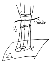
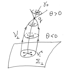
Figure 9: The volume element ${\cal V}_{\perp}$ of a parallelepiped on the hypersurface $\Sigma_{\perp}$ spanned by the frame vectors $\{\nu^{\alpha}_{i}\}$ of the orthonormal frame $\{u,\nu_{i}\}$ (5.44) is equal to the antisymmetric wedge product (9.128). The scalar $\theta$ measures the expansion of a small cloud of neighbouring geodesic trajectories forming a congruence of the volume ${\cal V}_{\perp}$ and as such measures contraction if $\theta<0$ or expansion if $\theta>0$. The figures show the conjugate points forming a one-dimensional ”rainbow” and ”focus” type caustics.

The proper time derivative of the transversal volume element ${\cal V}_{\perp}$ on the hypersurface $\Sigma_{\perp}$ will take the following form:

$$\dot{{\cal V}}=\dot{\rho_{1}}.....\rho_{3N-1}+....+\rho_{1}.....\dot{\rho}_{3N-1}=(\lambda_{1}+....+\lambda_{3N-1})~{}\rho_{1}...\rho_{3N-1}=Tr||u_{ij}||~{}{\cal V}=\theta~{}{\cal V}$$ (9.129)

or

$${1\over{\cal V}}{d{\cal V}\over ds}={d\ln{\cal V}\over ds}=\theta.$$ (9.130)

Thus the expansion scalar $\theta$ measures the fractional rate at which the volume of a small ball of particles forming a congruence is changing with respect to the time measured along the trajectory $\gamma(s)$. One can calculate the second derivative of the transversal volume:

$$\ddot{{\cal V}}=(\dot{\theta}+\theta^{2})~{}{\cal V}.~{}~{}~{}~{}~{}$$ (9.131)

Let us also introduce the volume element per particle as

$$\text{(volume per particle)}={\cal V}^{1\over 3N-1},$$ (9.132)

then

$$\ddot{{\cal V}^{1\over 3N-1}}={1\over 3N-1}\Big{(}\dot{\theta}+{1\over 3N-1}\theta^{2}\Big{)}~{}{\cal V}^{1\over 3N-1},$$ (9.133)

and the Raychaudhuri equation (9.125) can be written in the following form:

$$\ddot{{\cal V}^{1\over 3N-1}}={1\over 3N-1}~{}\Big{(}-R_{\alpha\beta}u^{\alpha}u^{\beta}-\theta^{\alpha\beta}\theta_{\alpha\beta}+\omega^{\alpha\beta}\omega_{\alpha\beta}\Big{)}~{}{\cal V}^{1\over 3N-1}.$$ (9.134)

Let us calculate the proper time derivative of the tensor $u_{ij}(s)$ defined in (5.52) on a curve $\gamma(s)$:

$${du_{ij}(s)\over ds} = {D(\nu^{\alpha}_{i}u_{\alpha;\beta}\nu^{\beta}_{j})\over ds}=\nu^{\alpha}_{i}{Du_{\alpha;\beta}\over ds}\nu^{\beta}_{j}=\nu^{\alpha}_{i}\Big{(}-u_{\alpha;\gamma}u^{\gamma}_{~{};\beta}-R_{\alpha\sigma\beta\gamma}u^{\sigma}u^{\gamma}+(u^{\gamma}u^{\alpha}_{~{};\gamma})_{;\beta}\Big{)}\nu^{\beta}_{j}=$$ (9.135)

$$= -u_{ik}u_{kj}-R_{ij}+\nu^{\alpha}_{i}(u^{\gamma}u^{\alpha}_{~{};\gamma})_{;\beta}\nu^{\beta}_{j},$$

where we used the equations (5.52) and (9.122). If the curve $\gamma(s)$ fulfils the geodesic equation $u^{\alpha}_{~{};\beta}u^{\beta}=0$, the last term vanishes, and we will get the Riccati equation for the matrix $u_{ij}(s)$:

$$\dot{u}_{ij}(s)+u_{ik}(s)u_{kj}(s)+R_{ij}(s)=0.$$ (9.136)

Using the representation of the metric tensor in the orthonormal frame coordinates $\{u^{\beta},\nu^{\alpha}_{i}\}$ (5.44) one can obtain useful representation for the scalar curvature $R$ in terms of sectional curvatures

$$R=g^{\alpha\gamma}g^{\beta\delta}R_{\alpha\beta\gamma\delta}=2\sum_{i}R_{\alpha\beta\gamma\delta}u^{\alpha}\nu^{\beta}_{i}u^{\gamma}\nu^{\delta}_{i}+\sum_{i,j}R_{\alpha\beta\gamma\delta}\nu^{\alpha}_{i}\nu^{\beta}_{j}\nu^{\gamma}_{i}\nu^{\delta}_{j}$$ (9.137)

or

$$R=2\sum_{i}K(u,\nu_{i})+2\sum_{i<j}K(\nu_{i},\nu_{j}),$$ (9.138)

where $K(\nu_{i},\nu_{j})$ is the sectional curvature of the 2-dimensional surface spanned by the vectors $(\nu_{i},\nu_{j})$ and $K(u,\nu_{i})$ is the sectional curvature of the 2-dimensional surface spanned by the vectors $(u,\nu_{i})$. This is the Riemann representation of the scalar curvature in terms of sectional-Gaussian curvatures (9.138) spanned by all pairs of orthonormal frame vectors. It is also true that

$$R=g^{\alpha\beta}R_{\alpha\beta}=R_{\alpha\beta}u^{\alpha}u^{\beta}+\sum_{i}R_{\alpha\beta}\nu^{\alpha}_{i}\nu^{\beta}_{i}~{}~{}~{}.$$ (9.139)

The last term can be further evaluated in the following way:

$$R_{\alpha\beta}\nu^{\alpha}_{i}\nu^{\beta}_{i}=g^{\gamma\delta}R_{\alpha\gamma\beta\delta}\nu^{\alpha}_{i}\nu^{\beta}_{i}=R_{\alpha\gamma\beta\delta}(u^{\gamma}u^{\delta}+\nu^{\gamma}_{j}\nu^{\delta}_{j})\nu^{\alpha}_{i}\nu^{\beta}_{i}=\sum_{i}K(u,\nu_{i})+2\sum_{i<j}K(\nu_{i},\nu_{j}).~{}~{}~{}~{}~{}~{}~{}~{}~{}~{}$$ (9.140)

From (9.139) we will have

$$R_{\alpha\beta}u^{\alpha}u^{\beta}=R-\sum_{i}R_{\alpha\beta}\nu^{\alpha}_{i}\nu^{\beta}_{i}$$ (9.141)

and then using the equations (9.138) and (9.140) we will get that

$$R_{\alpha\beta}u^{\alpha}u^{\beta}=\sum_{i}K(u,\nu_{i}).$$ (9.142)

This result tells us that the Ricci curvature term $R_{\alpha\beta}u^{\alpha}u^{\beta}$ in the Raychaudhuri equation (9.125) is a sum of sectional curvatures spanned by pairs of the velocity vector $u$ and all orthonormal frame vectors $\nu_{i}$. Thus the projection of the Ricci tensor on the orthonormal frame (9.140) and (9.142) can be expressed in terms of sectional curvatures. Using the equation (9.138) and the above equation (9.142) one can also obtain that

$$\sum_{i<j}K(\nu_{i},\nu_{j})={1\over 2}R-\sum_{i}K(u,\nu_{i})={1\over 2}R-R_{\alpha\beta}u^{\alpha}u^{\beta}=-(R_{\alpha\beta}-{1\over 2}Rg_{\alpha\beta})u^{\alpha}u^{\beta}.$$ (9.143)

In summary, we have the Jacobi equations (5.51) that describe the deviation of the geodesic trajectories and allow to investigate their stability and the Raychaudhuri equation (9.125) describing the global characteristics of the congruence of geodesic trajectories. Notice that in the evolution equations (5.51) and (9.125) the curvature appears in different forms. In the Jacobi deviation equations it is the sectional curvature (5.55) that plays a dominant role, while in the Raychaudhuri equation (9.125) the Ricci tensor is doing so.

10 Geodesic Focusing, Conjugate Points and Caustics

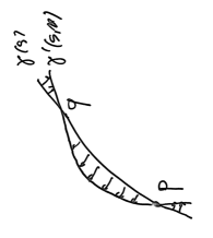
Figure 10: The left-hand figure shows the conjugate points $p$ and $q$ on the geodesic $\gamma(s)$ (10.144). The right-hand figure shows the congruence of geodesic trajectories of the two-dimensional Yang-Mills mechanical system ${\cal L}_{YM}={1\over 2}(\dot{x}^{2}+\dot{y}^{2})-{1\over 2}x^{2}y^{2}$ [47, 49, 50, 52, 53, 48, 54]. The trajectories start at the point $x=y=0$ and at different angles. As the angle varies the trajectories intersect one another on a clearly visible enveloping curve - one-dimensional analogues of caustic in geometrical optics (semi-cubical cusp singularity investigated by H. Whitney [30, 55, 86]). A caustic is defined as a curve to which the trajectories are tangent and at which the density of trajectories is large. The density is finite in the case of N-body system and the trajectories ”hit” the caustic with some delays.

If the solution $\delta q^{\alpha}_{\perp}$ of the Jacobi equations (5.51) vanishes at two distinct points $p$ and $q$ on a geodesic trajectory $\gamma(s)$, while not vanishing at all points of $\gamma(s)$, then $p$ and $q$ are called a pair of conjugate points (see Fig.10):

$$\delta q^{\alpha}_{\perp}(p)=0,~{}~{}~{}~{}~{}\delta q^{\alpha}_{\perp}(q)=0.$$ (10.144)

The conjugate points are characterised by the existence of a nonzero solution of the Jacobi equation that vanishes at the points $p$ and $q$ along the geodesic. Conjugate points, or focal points, are therefore the points that can be joined by a 1-parameter family of geodesics. The existence of conjugate points tells that the geodesics fail to be length-minimising. All geodesics are locally length-minimising, but not globally. This phenomenon arises when geodesics through $p$ encounter a caustic at $q$ showing that the frame coordinate system $\{u,\nu_{i}\}$ breaks down at $q$ and the corresponding Jacobian vanishes there [66, 67, 86, 104, 105]. Having a vanishing Jacobian on a curve on $Q^{3N}$ is referred to as a caustic. In this context the caustic could be defined as a set of points in the coordinate space $Q^{3N}$ conjugate to $p$ on geodesics through $p$. Equivalently one can define the caustic as an envelope of geodesics on $Q^{3N}$ through $p$ (see Figures 10, 12).

Using the concept of the transversal volume element ${\cal V}$ on the hypersurface $\Sigma_{\perp}$ introduced above in (9.128) and (9.130) one can derive the condition and criteria under which the conjugate points appear during the evolution of a dynamical system. A point $q$ is conjugate to a point $p$ on $\gamma(s)$ if and only if the volume element vanishes ${\cal V}(q)=0$ at $q$. Indeed, the frame coordinate system $\{u,\nu_{i}\}$ is always valid near $\gamma(s)$ until the conjugate point $q$ is reached, at the conjugate point $q$ the deviation vector $\delta q_{\perp}$ vanishes (10.144) and we have

$$\delta q^{\alpha}_{\perp}(q)=\sum^{3N-1}_{i=1}\rho_{i}\nu^{\alpha}_{i}=0.$$ (10.145)

This means that the linear combination of normal frame vectors $\nu^{\alpha}_{i}$ vanishes and the vectors become linearly dependent at the point $q$. The linear dependence can be expressed as a vanishing of the volume element ${\cal V}(q)=0$ at $q$ because the volume element is equal to the antisymmetric wedge product (9.128) of deviation vectors of the congruence $\{\gamma\}$. The vanishing of the volume element at $q$ characterises $q$ as a conjugate point. It follows that the expansion scalar $\theta$ given by a logarithmic derivative of the volume element (9.130)

$$\theta={d\ln{\cal V}\over ds}$$ (10.146)

is a continuous function at all points of $\gamma_{(}s)$ at which ${\cal V}\neq 0$, while $\theta$ becomes unbounded near point $q$ at which ${\cal V}=0$ with large and positive just to the future of $q$ and large and negative just to the past of $q$ on $\gamma_{(}s)$ (see Figs. 9, 14). Note that at $p$ itself $\delta q^{\alpha}_{\perp}(p)=0$ (10.144) and the above consideration remains valid as well, that is, the vanishing of the volume element at $p$ characterises it as a conjugate point ${\cal V}(p)=0$.

If at the point $q$ the $r$ linearly independent combinations of the $\nu^{\alpha}_{i}$ vanish, that is, at which there are $(3N-1)-r$ linearly independent vectors $\nu^{\alpha}_{i}$, the volume element in the infinitesimal neighbourhood of point $q$ will behave as ${\cal V}\sim s^{r}$. Such a point is said to have a conjugate degree $r$ with respect to $p$. Indeed, if at $q$ the $\rho_{i}(q)=0$ for $i=1,...,r$ and $\delta q^{\alpha}_{\perp}(q)=\sum^{3N-1}_{i=r+1}\rho_{i}(q)\nu^{\alpha}_{i}$ meaning that there are $(3N-1)-r$ linearly independent vectors $\nu^{\alpha}_{i}$ with nonzero coordinate derivatives $\dot{\rho}_{i}(q)=B_{i}\neq 0$, then near the point $q$ the coordinates are linear function of the proper time:

$$\rho_{i}(q)\sim A_{i}s,~{}~{}~{}i=1,...,r~{}~{}~{}~{}~{}~{}\rho_{j}(q)\sim B_{j}+A_{j}s,~{}~{}~{}j=r+1,...,3N-1,$$ (10.147)

where $A_{i}$,$B_{j}$ are integration constants and the volume element will behave as a power function of degree $r$:

$${\cal V}\sim\prod^{r}_{i=1}A_{i}s\prod^{3N-1}_{j=r+1}(B_{j}+A_{j}s)\sim s^{r}.$$ (10.148)

The expansion scalar (10.146) will scale at the conjugate point of degree $r$ as

$$\theta\sim{r\over s}.$$ (10.149)

Thus the congruence of geodesic trajectories intersect one another on a caustic, which is an enveloping hypersurface and is a high-dimensional analogue of a caustic surface in geometrical optics. The intersection of geodesic trajectories at the conjugate point creates a singularity. The distance between two neighbouring geodesic trajectories, intersecting each other at the point where they touch the caustic, tend to zero. The corresponding principal directions lies along the normals $\nu_{i},i=1,...,r$ to the high-dimensional hypersurface. These distances tend to zero as the first power of the distance along the normal directions from the point of intersection (see Fig.11). Thus in the high-dimensional space $Q^{3N}$ the caustic hypersurfaces can have rich morphology and a variety of dimensions. We will define below the dimension of the caustic hypersurfaces that are generated in high-dimensional coordinate space $Q^{3N}$.

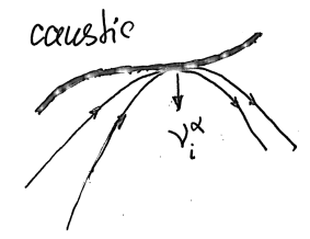
Figure 11: In the high dimensional coordinate space $Q^{3N}$ the caustic hypersurfaces can have a very reach morphology and variety of dimensions between zero and $3N-1$. The intersection of geodesic trajectories at the caustic creates a singularity because the transversal distance between two neighbouring geodesic trajectories tends to zero at the point where they ”touch” the caustic and the transversal volume element ${\cal V}_{\perp}$ vanishes (10.151). The remaining principal directions lies along the normals $\nu_{i}$ to the caustic hypersurface.

Let us consider the transversal deviations $\delta q^{\alpha}_{\perp}=\sum^{3N-1}_{i=1}\rho_{i}~{}\nu^{\alpha}_{i}$ (5.43) with the coordinates $\rho_{i}$ on the hypersurface $\Sigma_{\perp}$ that is spanned by the normal vectors $\{\nu^{\alpha}_{i}\}$ of the orthonormal frame $\{u^{\beta},\nu^{\alpha}_{i}\}$ (5.44) (see Fig. 9). The volume element of a parallelepiped on the hypersurface $\Sigma_{\perp}$ was defined as the antisymmetric wedge product ${\cal V}_{\perp}=\prod_{\alpha}\wedge\delta q^{\alpha}_{\perp}=\rho_{1}...\rho_{3N-1}$ (9.128). The Maupertuis’s metric (2.8) projected onto the hypersurface $\Sigma_{\perp}$ normal to the velocity vector $u$ will have the following form:

$$ds^{2}_{\perp}=|\delta q_{\perp}|^{2}=g_{\alpha\beta}\delta q^{\alpha}_{\perp}\delta q^{\beta}_{\perp}=\sum^{3N-1}_{i=1}\rho^{2}_{i},$$ (10.150)

where we used the fact that $(\nu_{i}\cdot\nu_{j})=\delta_{ij}$ (5.44). If in the vicinity of a caustic $r$ transversal deviation vectors (10.147) tend to zero $\rho_{i}\rightarrow 0,i=1,...,r$, then we will have

$$ds^{2}_{\perp}=\sum^{(3N-1)-r}_{i=1}\rho^{2}_{i},~{}~{}~{}~{}~{}~{}~{}~{}~{}~{}~{}{\cal V}_{\perp}\propto\rho_{1}...\rho_{r}\rightarrow 0$$ (10.151)

meaning that the caustic hypersurface has the dimension $(3N-1)-r$. The index $r$ defined as a conjugate degree has a dynamical origin and can by calculated be solving the equation (5.51) that includes the tensor $R_{ij}$ given in (7.84).

The question is how the high-dimensional caustics generated in the extended coordinate space $Q^{3N}$ are connected with the caustics in the physical three-dimensional space. Let us consider the perturbation $\delta q^{\alpha}$ of the geodesic trajectories that appear due to the variation of the particle masses $M^{1/2}_{a}\rightarrow M^{1/2}_{a}+\delta M^{1/2}$ and $M^{1/2}_{b}\rightarrow M^{1/2}_{b}+\delta M^{1/2}$. It follows from (2.6) that

$$\delta q^{\alpha}_{ab}=(0,...,\vec{r}_{a},...,\vec{r}_{b},...,0)\delta M^{1/2}$$ (10.152)

and the length of the perturbation $|\delta q|^{2}=g_{\alpha\beta}\delta q^{\alpha}\delta q^{\beta}$ is

$$|\delta q_{ab}|^{2}=W(\vec{r}^{~{}2}_{a}+\vec{r}^{~{}2}_{b})\delta M.$$ (10.153)

The distance between particles $r_{ab}$ is bounded from above by the expression

$$|\vec{r}_{a}-\vec{r}_{b}|^{2}\leq 2(\vec{r}^{~{}2}_{a}+\vec{r}^{~{}2}_{b})={2\over W\delta M}|\delta q_{ab}|^{2}$$ (10.154)

and tends to zero if $|\delta q_{ab}|^{2}$ approaches a conjugate point. In general if in the vicinity of a caustic $r$ deviation vectors (10.147) tend to zero $\rho_{i}\rightarrow 0,i=1,...,r$, then it follows that a subsystem of at least of $r$ particles of an N-body system will converge to a caustic hypersurface in the three-dimensional physical space. The perturbation of all $N$ particles will lead to the following inequality:

$$\sum^{N}_{a<b}|\vec{r}_{a}-\vec{r}_{b}|^{2}\leq 2(N-1)\sum^{N}_{a=1}\vec{r}^{~{}2}_{a}={2(N-1)\over W\delta M}|\delta q_{N}|^{2},$$ (10.155)

and if $|\delta q_{N}|^{2}$ tends to zero then the geodesics of an N-body system will converge to a focus in the three-dimensional physical space.

Figure 12: The figure shows the congruence of geodesic trajectories $\{\gamma(s)\}$ of the two-dimensional Yang-Mills mechanical system ${\cal L}_{YM}={1\over 2}(\dot{x}^{2}+\dot{y}^{2})-{1\over 2}x^{2}y^{2}$ [47, 49, 50] that are all orthogonal to the line $x=0$. It is an example of a hypersurface $\Sigma_{\perp}$, which in the case of Yang-Mills mechanics is a one-dimensional line $x=0$. This figure illustrates the concept of a conjugate point to a hypersurface $\Sigma_{\perp}$ that was discussed after formula (10.149). The locus of such conjugate points, as $\gamma(s)$ varies, form the caustics, clearly visible in the figure. As the trajectories evolve in time from the left of the figure to the right the structure of the caustics and their location is changing. The time slices of the congruence show metamorphosis of caustics as they appear at different time slices. During the evolution of trajectories, the expansion scalar $\theta$ changes from contraction $\theta<0$ to the expansion $\theta>0$ and again to contraction. The further evolution of trajectories is shown in Fig.13.

There is an alternative way of defining the conjugate points that is useful in describing the congruence of geodesics that exhibits a zero vorticity of their collective spin [66, 67, 104, 105]. Suppose, that $\gamma_{0}$ is a geodesic orthogonal to a hypersurface $\Sigma_{\perp}$ at the point $p$ and let us consider the congruence of geodesics $\{\gamma\}$ that meet $\Sigma_{\perp}$ orthogonally and lie in a small neighbourhood of $\gamma_{0}$. A point $q$ is conjugate to $\Sigma_{\perp}$ on $\gamma_{0}$ when a nontrivial Jacobi field exists on $\gamma_{0}$ that vanishes at $q$ but not everywhere along $\gamma_{0}$ and that arises from a one-parameter system of geodesics $\{\gamma\}$ that are all orthogonal to $\Sigma_{\perp}$ at their intersection with $\Sigma_{\perp}$. A locus of such conjugate points when $\gamma$ varies forms a caustic (see Fig.9 and Fig.12). Thus here as well a caustic is a curve, surface or hypersurface to which each of the geodesic trajectories is tangent, defining a boundary of an envelope of trajectories on which the density of particles of an N-body system is large. The caustics are formed in the regions where a sufficient number of particles is concentrated causing that regions to be much denser with particles than the background space. The concept of a caustic generated by a geodesic congruence that is normal to a surface is important because it defines a geodesic flow without vorticity:

$$\omega_{\alpha\beta}=0,$$ (10.156)

that is exhibiting an absence of their collective spin. The demonstration of this fact is given in Appendix E. In that case the Raychaudhuri equation will reduce to the following form [58, 66, 67]:

$${d\theta\over ds}=-R_{\alpha\beta}u^{\alpha}u^{\beta}-{1\over 3N-1}\theta^{2}-\theta_{\alpha\beta}\theta^{\alpha\beta},$$ (10.157)

and the equation for the volume element (9.134) can be written as

$$\ddot{{\cal V}^{1\over 3N-1}}=-{1\over 3N-1}\Big{(}R_{\alpha\beta}u^{\alpha}u^{\beta}+\theta^{\alpha\beta}\theta_{\alpha\beta}\Big{)}{\cal V}^{1\over 3N-1}.$$ (10.158)

In the case of spherically symmetric expansion the shear tensor vanishes, $\theta^{\alpha\beta}=0$, and we have the equations of fundamental importance:

$${d\theta\over ds}=-R_{\alpha\beta}u^{\alpha}u^{\beta}-{1\over 3N-1}\theta^{2},~{}~{}~{}~{}~{}~{}\ddot{{\cal V}^{1\over 3N-1}}=-{1\over 3N-1}R_{\alpha\beta}u^{\alpha}u^{\beta}~{}{\cal V}^{1\over 3N-1}.$$ (10.159)

The criteria under which a conjugate point to a surface $\Sigma_{\perp}$ will appear during the evolution of a dynamical system are similar to the ones obtained above and are based on the behaviour of the volume element ${\cal V}$ on the hypersurface $\Sigma_{\perp}(s)$ introduced in (9.128) and (9.130). The frame coordinate system $\{u,\nu_{i}\}$ is always valid near $\gamma_{0}(s)$ until the conjugate point $q$ is reached. A point $q$ is conjugate to a surface $\Sigma_{\perp}$ on $\gamma_{0}$ if and only if ${\cal V}=0$ at $q$. The expansion scalar $\theta$ is a continuous function at all points of $\gamma_{0}$ at which ${\cal V}\neq 0$, while $\theta$ becomes unbounded near the point $q$ at which ${\cal V}=0$. This characterises $q$ as a conjugate point to a surface $\Sigma_{\perp}$ and because of the relation (9.130) the expansion scalar $\theta$ will tend to infinities $\pm\infty$ when ${\cal V}$ approaches the zero value (see Fig.14). When the surface $\Sigma_{\perp}$ degenerates to a single point $p$, the congruence $\{\gamma\}$ will consist of geodesics through $p$ and the above criteria reduce to the criteria for the geodesics emanating from a single point $p$.

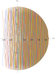
Figure 13: The figure shows the evolution of the congruence of geodesic trajectories of the two-dimensional Yang-Mills mechanical system $H_{YM}={1\over 2}(\dot{p_{x}}^{2}+\dot{p_{y}}^{2})+{1\over 2}x^{2}y^{2}$ for a longer period of time compared to the one shown in Fig.12. The trajectories chaotically fill out the available regions in the coordinate $(x,y)$ and momentum $(p_{x},p_{y})$ planes [47, 49, 50].

The important conclusion that can be drawn from the Raychaudhuri equation (9.125) is that if

$$R_{\alpha\beta}u^{\alpha}u^{\beta}+\theta^{\alpha\beta}\theta_{\alpha\beta}-\omega^{\alpha\beta}\omega_{\alpha\beta}\geq 0$$ (10.160)

the solution will lead to the geodesic focusing and generation of caustics. Indeed, with the initial negative value of $\theta(0)<0$ and $\dot{\theta}$ negative, the solution for the expansion scalar (9.125) will tend to the negative infinity $\theta(s)\rightarrow-\infty$ due to the Sturm-Picone comparison theorem. For the congruence of geodesics that have zero vorticity (10.156) the criteria (10.160) will reduce to the condition

$$R_{\alpha\beta}u^{\alpha}u^{\beta}\geq 0.$$ (10.161)

In the next section we will demonstrate that the above criteria (10.161) are fulfilled in the case of self-gravitating N-body systems.

11 Geodesic Focusing, Caustics and Large Scale Structure

The Ranchanduri equation (10.157) for the volume expansion scalar $\theta$ allows to investigate the appearance of caustics, the regions of the coordinate space where the density of particles is much higher than the average particle density. The first term of the Ranchanduri equation (9.125), (10.157) and (10.159) contains the quadratic form $R_{\alpha\beta}u^{\alpha}u^{\beta}$ of the Ricci tensor (9.140), (9.141), (9.142) contracted with the velocity vector $u^{\alpha}$. It defines the evolution of the volume element through the equation (9.130) and the criteria (10.161). We can find the Ricci tensor contracting the Riemann tensor in the Maupertuis’s metric (2.8). It has the following form:

$$R_{\alpha\beta\gamma\delta} = {1\over 2W}(g_{\alpha\delta}W_{\beta\gamma}-g_{\alpha\gamma}W_{\beta\delta}+g_{\beta\gamma}W_{\alpha\delta}-g_{\beta\delta}W_{\alpha\gamma})-$$ (11.162)

$$- {3\over 4W^{2}}(g_{\alpha\delta}W_{\beta}W_{\gamma}-g_{\alpha\gamma}W_{\beta}W_{\delta}+g_{\beta\gamma}W_{\alpha}W_{\delta}-g_{\beta\delta}W_{\alpha}W_{\gamma})+$$

$$+ {1\over 4W^{2}}(g_{\alpha\delta}g_{\beta\gamma}-g_{\alpha\gamma}g_{\beta\delta})W_{\sigma}W^{\sigma},$$

where $W_{\alpha}={\partial W\over\partial q^{\alpha}},~{}~{}~{}W_{\alpha\beta}={\partial^{2}W\over\partial q^{\alpha}\partial q^{\beta}}.$ It is a universal expression that is valid for any dynamical system that is described by an interaction potential $U(q)$ of a general form that may also include an additional external background potential. We can obtain the corresponding Ricci tensor $R_{\alpha\beta}$ by contracting the indices:

$$R_{\alpha\beta}=g^{\gamma\delta}R_{\alpha\gamma\beta\delta} = -{3N-2\over 2W}\Big{(}W_{\alpha\beta}+g_{\alpha\beta}{W_{\sigma}^{~{}\sigma}\over 3N-2}\Big{)}+$$ (11.163)

$$+ {3(3N-2)\over 4W^{2}}\Big{(}W_{\alpha}W_{\beta}-{3N-4\over 3(3N-2)}g_{\alpha\beta}W_{\sigma}W^{\sigma}\Big{)},$$

and the scalar curvature $R$ by the second contraction:

$$R=g^{\alpha\beta}R_{\alpha\beta} = 3N(3N-1)\Big{[}-{W_{\sigma}^{~{}\sigma}\over 3NW}-\Big{(}{1\over 4}-{1\over 2N}\Big{)}{W_{\sigma}W^{\sigma}\over W^{2}}\Big{]}.$$ (11.164)

We can find the quadratic form $R_{\alpha\beta}u^{\alpha}u^{\beta}$ by using the expression for the Ricci tensor (11.163) and contracting it with the velocity vectors:

$$R_{\alpha\beta}u^{\alpha}u^{\beta} = -{3N-2\over 2W}\Big{(}(uW^{{}^{\prime\prime}}u)+{1\over 3N-2}|W^{{}^{\prime\prime}}|\Big{)}+{3(3N-2)\over 4W^{2}}\Big{(}(uW^{{}^{\prime}})^{2}-{3N-4\over 3(3N-2)}|W^{{}^{\prime}}|^{2}\Big{)}.~{}~{}~{}~{}~{}~{}~{}~{}~{}~{}~{}~{}$$ (11.165)

The Raychaudhuri equation (10.157) will take the following form:

$${d\theta\over ds}= - {3(3N-2)\over 4W^{2}}\Big{(}(uW^{{}^{\prime}})^{2}-{3N-4\over 3(3N-2)}|W^{{}^{\prime}}|^{2}\Big{)}-{1\over 3N-1}\theta^{2}-\theta_{\alpha\beta}\theta^{\alpha\beta}+$$ (11.166)

$$+ {3N-2\over 2W}\Big{(}(uW^{{}^{\prime\prime}}u)+{1\over 3N-2}|W^{{}^{\prime\prime}}|\Big{)}.$$

The first two terms are proportional to the second order derivatives acting on the potential function (7.74), and they have been discussed and calculated in (7). They are suppressed compared to the first-order derivative terms, therefore the sign of the quadratic form in collisionless systems will be defined by the first order derivative terms:

$$R_{\alpha\beta}u^{\alpha}u^{\beta}={3(3N-2)\over 4W^{2}}\Big{(}(uW^{{}^{\prime}})^{2}-{3N-4\over 3(3N-2)}|W^{{}^{\prime}}|^{2}\Big{)}.$$

We can express the quadratic form in terms of angle $\theta_{u}$ introduced earlier in (7.78):

$$R_{\alpha\beta}u^{\alpha}u^{\beta} = {3(3N-2)\over 4W^{2}}\Big{(}\cos^{2}\theta_{u}-{1-{4\over 3N}\over 3-{6\over 3N}}\Big{)}|W^{{}^{\prime}}|^{2}$$ (11.167)

and find out the maximum and minimum values of the Ricci quadratic form:

$$R_{\alpha\beta}u^{\alpha}u^{\beta}|_{max} = +{(3N-1)\over 2W^{2}}|W^{{}^{\prime}}|^{2}~{}~{}~{}~{}~{}~{}R_{\alpha\beta}u^{\alpha}u^{\beta}|_{min}=-{(3N-4)\over 4W^{2}}|W^{{}^{\prime}}|^{2}.$$ (11.168)

The geodesic focusing effect will appear when the quadratic form $R_{\alpha\beta}u^{\alpha}u^{\beta}$ is positive-definite and the criteria (10.161) is fulfilled. Its value controls the time scale at which the self-gravitating system will develop geodesic focusing and caustics, the regions in the coordinate space where the density of particles is large. In that case the Raychaudhuri equation will take the following form:

$${d\theta\over ds}=-{(3N-1)\over 2W^{2}}|W^{{}^{\prime}}|^{2}-{1\over 3N-1}\theta^{2}-\theta^{\alpha\beta}\theta_{\alpha\beta}.$$ (11.169)

Because the last term $\theta^{\alpha\beta}\theta_{\alpha\beta}$ is positive-definite, we will have the inequality

$${d\theta\over ds}\leq-(3N-1){|W^{{}^{\prime}}|^{2}\over 2W^{2}}-{1\over 3N-1}\theta^{2}.$$ (11.170)

In the case of spherically symmetric evolution $\theta^{\alpha\beta}=0$ [106] and the equation will take the following form:

$$~{}~{}~{}~{}~{}{d\theta\over ds}=-(3N-1){(\nabla W)^{2}\over 2W^{3}}-{1\over 3N-1}\theta^{2},$$ (11.171)

where the first term on the r.h.s can be expressed in terms of the gradient of the potential function (7.75). When the number of particles is large $N\gg 1$ we will have

$$~{}~{}~{}~{}~{}{d\theta\over ds}=-3N{(\nabla W)^{2}\over 2W^{3}}-{1\over 3N}\theta^{2}.$$ (11.172)

It is convenient to introduce the function $B^{2}$

$$B^{2}(s)=(3N)^{2}{(\nabla W)^{2}\over 2W^{3}}$$ (11.173)

so that the equation (11.172) will take the following form:

$$~{}~{}~{}~{}~{}{d\theta\over ds}=-{1\over 3N}(\theta^{2}+B^{2}(s)).$$ (11.174)

The $B^{2}(s)$ is a positive decreasing function of proper time $s$ and is bounded from below. We will integrate the above equation in the approximation when the function $B^{2}(s)$ is taken in its minimum value $B^{2}_{min}(s)=B^{2}$. In that case the solution for the expansion scalar $\theta(s)$ is

$$\theta(s)=B\tan\Big{(}\arctan{\theta(0)\over B}-{B\over 3N}s\Big{)},$$ (11.175)

where $\theta(0)$ is the initial value of the expansion scalar. The expansion scalar $\theta(s)$ becomes singular at the proper times $s_{n}$:

$$s_{caustics}={3N\over B}\Big{(}\arctan{\theta(0)\over B}+{\pi\over 2}+\pi n\Big{)},~{}~{}~{}~{}n=0,\pm 1,\pm 2,...$$ (11.176)

As far as the expansion scalar $\theta(s)$ tends to infinity at a certain epoch $s_{caustics}$, it follows that the volume element that is occupied by the galaxies decreases and tends to zero creating the regions in space of large galactic densities. Indeed, let us calculate the evolution of the volume element. We can find the time dependence on the volume element ${\cal V}$ by integrating the equation (10.146):

$$d\ln{\cal V}=\theta ds=d\Big{(}3N\ln\cos\Big{[}\Big{(}\arctan{\theta(0)\over B}-{B\over 3N}s\Big{)}\Big{]}\Big{)},$$ (11.177)

and thus

$${\cal V}(s)={\cal V}(0)\Big{[}{\cos\Big{(}\arctan{\theta(0)\over B}-{B\over 3N}s\Big{)}\over\cos\Big{(}\arctan{\theta(0)\over B}\Big{)}}\Big{]}^{3N}.$$ (11.178)

It follows that the volume element occupied by galaxies tends to zero at each epoch defined by the $s_{n}$ in (11.176) (see Fig.14). As we already discussed in the ninth section, the vanishing of the volume element characterises the appearance of conjugate points and caustics. The density of galaxies defined as $\rho_{g}(s)=NM_{g}/{\cal V}(s)$ allows to calculate the density contrast $\delta=\delta\rho/\rho$ as it was defined above in (8.110) and (8.111). The ratio of densities during the evolution from the initial volume ${\cal V}(0)$ to the volume ${\cal V}(s)$ at the epoch $s$ will give us the density contrast:

$$\delta_{caustics}(s)+1={\rho(s)\over\rho(0)}={{\cal V}(0)\over{\cal V}(s)}=\Big{[}{\cos\Big{(}\arctan{\theta(0)\over B}\Big{)}\over\cos\Big{(}\arctan{\theta(0)\over B}-{B\over 3N}s\Big{)}}\Big{]}^{3N}.$$ (11.179)

As one can see, at the epoch (11.176) where the expansion scalar $\theta(s)$ becomes singular, the trigonometric function in the denominator tends to zero and the density contrast is increasing and tends to infinity, the phenomenon similar to the spherical top-hat model. One can calculate the volume element per galaxy defined in (9.134), (10.158), thus

$${\cal V}(s)^{{1\over 3N}}={\cal V}(0)^{{1\over 3N}}~{}{\cos\Big{(}\arctan{\theta(0)\over B}-{B\over 3N}s\Big{)}\over\cos\Big{(}\arctan{\theta(0)\over B}\Big{)}}.$$ (11.180)

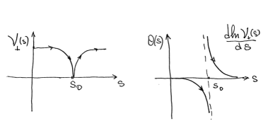
Figure 14: The figures show the behaviour of the volume element ${\cal V}_{\perp}(s)$ and of the expansion scalar $\theta$ in the vicinity of a caustic. A similar behaviour takes place at each epoch $s_{caustics}$ (11.182).

In order to illustrate the above results let us consider the evolution of galaxies occupying the volume ${\cal V}(0)$ and starting without expansion $d{\cal V}(s)/ds|_{s=0}=0$, thus $\theta(0)=0$, and we will get for the scalar $\theta(s)$ the expression

$$\theta(s)=-B\tan\Big{(}{B\over 3N}s\Big{)}.$$ (11.181)

At each of the epochs

$$s_{caustics}={3\pi N\over 2B}(1+2n),~{}~{}~{}~{}n=0,\pm 1,\pm 2,...$$ (11.182)

the expansion scalar $\theta$ has the following asymptotic:

$$s\rightarrow s_{caustics},~{}~{}~{}~{} \theta(s)\approx{3N\over s-s_{caustics}}-{B^{2}\over 9N}(s-s_{caustics})+...$$ (11.183)

and becomes unbounded near $s_{caustics}$ at which ${\cal V}=0$ (see Figs. 9, 14). The conjugate degree $r$ defined in (10.149) for the caustic (11.183) has the maximal value

$$r=3N.$$ (11.184)

The above equations show that in a self-gravitational N-body system the caustics can be generated periodically during the expansion of the Universe as it follows from the equation (11.181). Let us estimate the time scale of the appearance of the first caustic in (11.176). For $s_{caustics}$ we have the following expression:

$$s_{caustics}=\pi{3N\over 2B}.$$ (11.185)

In terms of physical time (2.12) the characteristic time scale of generation of gravitational caustics is

$$\tau_{caustics}={3\pi N\over 2B\sqrt{2}W}={\pi\over 2}\sqrt{{W\over(\nabla W)^{2}}}.$$ (11.186)

We can evaluate the quantities entering into this equation by considering a self-gravitating system of $N$ galaxies of the mass $M_{g}$ each. The kinetic energy $W$ of the galaxies was found in (8.101) and the square of the force acting on a unit mass of the galaxies $(\nabla W)^{2}$ in (8.102). Thus we will obtain

$$\tau_{caustics}={\alpha^{{}^{\prime}}\over 4\pi G\rho(t)}H(t),$$ (11.187)

where the numerical coefficient $\alpha^{{}^{\prime}}={3\pi\over 2\sqrt{2}}$. It is in a good agreement with our previous result, (8.98) and (8.103), obtained by solving the Jacobi equation (5) and by using the expressions (7.81) and (7.83) for the sectional curvatures. The volume element (11.180) will take the following form:

$${\cal V}(s)={\cal V}(0)\Big{[}\cos\Big{(}{B\over 3N}s\Big{)}\Big{]}^{3N},$$ (11.188)

and it is oscillating between ${\cal V}(0)$ and zero values. The conjugate degree $r$ defined in (10.148) is as well equal to $3N$. The density contrast (11.179) takes the following form:

$$\delta_{caustics}+1={1\over\Big{[}\cos\Big{(}{B\over 3N}s\Big{)}\Big{]}^{3N}},$$ (11.189)

and it has the following asymptotic in the vicinity of a caustic:

$$\delta_{caustics}(s)\approx\Big{[}{3N\over B(s-s_{caustics})}\Big{]}^{3N}+...$$ (11.190)

From the equation (11.173) we have ${3N\over B}=\sqrt{{2W^{3}\over(\nabla W)^{2}}}$, and the density contrast on the caustic increases:

$$\delta_{caustics}(t)\approx\Big{[}\sqrt{{W\over(\nabla W)^{2}}}{1\over(t-{\pi\over 2}\sqrt{{W\over(\nabla W)^{2}}})}\Big{]}^{3N}=\Big{[}{2\over\pi}{\tau_{caustic}\over(t-\tau_{caustic})}\Big{]}^{3N}~{}.$$ (11.191)

Thus galaxies will contract into a caustic, a high-density lump, and then expand again if the system remains gravitationally unbound. One can conjecture that during a contraction into a caustic, a close encounter of galaxies will eject away some of them, so that this ”evaporation” will take out part of the total energy [70, 71, 75] and the rest of the system will evolve into a gravitationally bound galactic cluster. The maximal density contrast that can be achieved in the spherical top-hat model of Gunn and Gott [76] is about $18\pi^{2}$ (8.113) and the density contrast in the vicinity of the caustics is given in (11.189), (11.191) and can be even larger. It would be interesting to compare the theoretical result (11.189) with the results of the numerical simulations of the density contrast and of that obtained from the observational data.

We conclude that a self-gravitating N-body system can develop gravitational caustics, surfaces and filaments on which the density of galaxies is higher than the average density of matter in the expanding Universe.

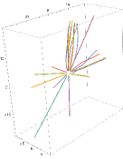
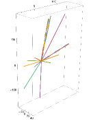
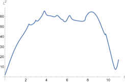
Figure 15: These figures illustrate the generation of a caustic. The left figure shows the initial stage of the radial expansion of a self-gravitating system of $N=20$ particles, with nine particles in the ”north pole” congruence. The figure in the middle shows the same system of particles when the integration time interval was extended from $\triangle t=4$ to a longer time interval $\triangle t=11$. The figure in the right shows the time dependence of the sum of the square distances $L^{2}$ between nine particles of the congruence.

12 Conclusions

In this paper we demonstrated the generation of gravitational caustics, which appear due to the gravitational geodesic focusing in a self-gravitating N-body system and are space regions where the density of particles is higher than the average density in the Universe. We considered the physical conditions at which a self-gravitating system is developing geodesic focusing and caustics by investigating the Jacobi and Ranchandhuri equations for self-gravitating N-body systems. By solving these equations we estimated the characteristic relaxation time scales, the time scale of generation of gravitational caustics, and calculated the density contrast on the caustics. It is suggested that the intrinsic mechanism of caustics generation is responsible for the formation of cosmological large-scale structures that consist of matter concentrations in the form of galactic clusters, filaments, and vast regions devoid of galaxies.

In our approach the dynamics of a self-gravitating N-body system was formulated in terms of a geodesic flow on a curved Riemannian manifold, and we were investigating the signs of the sectional curvatures that define the stability of geodesic trajectories in different parts of the phase space. The regions of negative sectional curvatures are responsible for the exponential instability of geodesic trajectories, deterministic chaos, and relaxation phenomena of globular clusters and galaxies, while the regions of positive sectional curvatures are responsible for the gravitational geodesic focusing and generation of caustics.

The dynamical properties of self-gravitating N-body systems crucially depend of the behaviour of the sectional curvature $K(q,u,\delta q_{\perp})$. The formulas derived in the article allow to investigate the sectional curvatures not only analytically, but they are also convenient for the analysis of the numerical simulations. In particular, the behaviour of the matter power spectrum at small scales $k\geq 2\times 10^{-2}[h~{}\text{Mps}^{-1}]$ shown in Fig. 3 has a non-perturbative character because in that region the matter density contrast $\delta$ is large and cannot be described by the perturbation theory. Only the numerical simulations allow to investigate that region of small scales. The maximal density contrast that is achievable in the spherical top-hat model of Gunn and Gott [76] is about $18\pi^{2}$ (8.113), and the density contrast in the vicinity of the caustics is given in (11.189) and can be even larger. It would be interesting to compare this theoretical result with the results of the numerical simulations of the density contrast and of that from the observational data.

Acknowledgement. I would like to thank Konstantin Savvidy for stimulating discussions clarifying the physical context of gravitational geodesic focusing and generation of caustics.

Appendix A Curvature Tensors

The Riemann and Weyl curvature tensors express the tidal force that acts on the interacting particles when they move along the geodesic trajectories. The Weyl tensor differs from the Riemann curvature tensor in that it does not convey information on how the volume of the congruence changes, but rather only how the shape of the congruence is distorted by the tidal force. Thus the Weyl tensor defines the shear and the rotation, but does not define the distances and volume evolutions. Let us consider the relation between the Riemann and Ricci curvature tensors and the Weyl tensor in the case of Maupertuis’s metric (2.8). The Weyl tensor can be represented in terms of the Riemann tensor and a polynomial, which is a linear combination of the Ricci tensor and the scalar curvature:

$$C_{\alpha\delta\beta\gamma} = R_{\alpha\delta\beta\gamma}+{1\over 3N-2}(g_{\alpha\gamma}R_{\delta\beta}-g_{\alpha\beta}R_{\delta\gamma}+g_{\delta\beta}R_{\alpha\gamma}-g_{\delta\gamma}R_{\alpha\beta})+$$ (1.192)

$$+ {1\over(3N-1)(3N-2)}(g_{\alpha\beta}g_{\delta\gamma}-g_{\alpha\gamma}g_{\delta\beta})R.$$

On the coordinate space $Q^{3N}$ that is supplied by the Maupertuis’s metric (2.8) we can calculate the Weyl tensor by substituting the expressions for $R_{\alpha\beta\gamma\delta}$ (11.162), $R_{\alpha\beta}$ (11.163) and $R$ (11.164) into (1.192), and one can get convinced that the Weyl tensor vanishes:

$$C_{\alpha\delta\beta\gamma} = 0,$$ (1.193)

meaning that the Maupertuis’s metric (2.8) is conformally flat metric. Due to the fact that the Weyl tensor vanishes (1.193) it follows from (1.192) that the Riemann tensor can be expressed in terms of Ricci tensor $R_{\alpha\beta}$ and scalar curvature $R$:

$$R_{\alpha\beta\gamma\delta} = {1\over 3N-2}(g_{\alpha\gamma}R_{\beta\delta}-g_{\alpha\delta}R_{\beta\gamma}+g_{\beta\delta}R_{\alpha\gamma}-g_{\beta\gamma}R_{\alpha\delta})+$$ (1.194)

$$+ {1\over(3N-1)(3N-2)}(g_{\alpha\delta}g_{\beta\gamma}-g_{\alpha\gamma}g_{\beta\delta})R.$$

By using the above representation (1.194) of the Riemann tensor one can express the sectional curvatures (5.55) appearing in the Jacobi equations (5.51), (5.52) and in (5) in terms of the Ricci tensor and scalar curvature:

$$R_{\alpha\beta\gamma\delta}\delta q^{\alpha}_{\perp}u^{\beta}\delta q^{\gamma}_{\perp}u^{\delta}={1\over 3N-2}\Big{(}(uRu)~{}|\delta q_{\perp}|^{2}+(\delta q_{\perp}R\delta q_{\perp})-{1\over(3N-1)}R|\delta q_{\perp}|^{2}\Big{)},~{}~{}$$ (1.195)

where $(uRu)=u^{\beta}R_{\beta\delta}u^{\delta},~{}~{}(\delta q_{\perp}R\delta q_{\perp})=\delta q^{\alpha}_{\perp}R_{\alpha\gamma}\delta q^{\gamma}_{\perp}.$ The tensor $R_{ij}$ in (5.52) will take the following form:

$$R_{ij} = R_{\alpha\beta\gamma\delta}\nu^{\alpha}_{i}u^{\beta}\nu^{\gamma}_{j}u^{\delta}={1\over 3N-2}\Big{(}R_{\beta\delta}u^{\beta}u^{\delta}\delta_{ij}+R_{\alpha\gamma}\nu^{\alpha}_{i}\nu^{\gamma}_{j}-{1\over(3N-1)}R\delta_{ij}\Big{)}.$$ (1.196)

By using the metric tensor in the orthonormal frame $\{u^{\beta},\nu^{\alpha}_{i}\}$ (5.44) we can obtain the expression for the tensor $R_{ij}$ that involves only the normal frame vectors $\{\nu^{\alpha}_{i}\}$:

$$R_{ij} = R_{\alpha\beta\gamma\delta}\nu^{\alpha}_{i}u^{\beta}\nu^{\gamma}_{j}u^{\delta}={1\over 3N-2}R_{\alpha\beta}(\nu^{\alpha}_{i}\nu^{\beta}_{j}-\delta_{ij}\ \nu^{\alpha}_{k}\nu^{\beta}_{k})+{1\over(3N-1)}R\delta_{ij}.$$ (1.197)

The useful relation can be obtained by taking the trace of the matrix $R_{ij}$:

$$Tr||R_{ij}||=\delta^{ij}R_{\alpha\beta\gamma\sigma}\nu^{\alpha}_{i}u^{\beta}\nu^{\gamma}_{j}u^{\sigma}=R_{\alpha\beta\gamma\sigma}\nu^{\alpha}_{i}u^{\beta}\nu^{\gamma}_{i}u^{\sigma}=R_{\alpha\beta\gamma\sigma}u^{\beta}u^{\sigma}(g^{\alpha\gamma}-u^{\alpha}u^{\gamma})=R_{\beta\sigma}u^{\beta}u^{\sigma}.$$ (1.198)

It is the term of the Ranchanduri equation (9.125), (10.157) that contains the quadratic form of the Ricci tensor (9.140), (9.141), (9.142). We also have

$$R_{ij} = -{1\over 2W}\Big{(}\delta_{ij}(uW^{{}^{\prime\prime}}u)+(\nu_{i}W^{{}^{\prime\prime}}\nu_{j})\Big{)}+{3\over 4W^{2}}\Big{(}\delta_{ij}(uW^{{}^{\prime}})^{2}+(\nu_{i}W^{{}^{\prime}})(\nu_{j}W^{{}^{\prime}})\Big{)}-{1\over 4W^{2}}\delta_{ij}|W^{{}^{\prime}}|^{2}.$$

The initial frame vectors $\{\nu^{\alpha}_{i}\}$, $i=1,...,3N-1$ can be defined in the following form:

$$\nu^{\alpha}_{1}(0)=(\vec{\nu}_{1},0,...,0){1\over\sqrt{W}},$$

$$..........,$$

$$\nu^{\alpha}_{N}(0)=(0,0,...,\vec{\nu}_{N}){1\over\sqrt{W}}$$

$$\nu^{\alpha}_{2N+1}(0)\propto(M^{1/2}_{2}\dot{\vec{r}}^{~{}2}_{2}~{}\dot{\vec{r}}_{1},-M^{1/2}_{1}\dot{\vec{r}}^{~{}2}_{1}~{}\dot{\vec{r}}_{2},0,...,0),$$

$$...........,$$

$$\nu^{\alpha}_{3N-1}(0)\propto(M^{1/2}_{N}\dot{\vec{r}}^{~{}2}_{N}~{}\dot{\vec{r}}_{1},0,...,0,-M^{1/2}_{1}\dot{\vec{r}}^{~{}2}_{1}~{}\dot{\vec{r}}_{N}).$$ (1.200)

These vectors are orthogonal to $u^{\alpha}(0)={1\over\sqrt{2}W}(M^{1/2}_{1}\dot{\vec{r}}_{1}(0),...,M^{1/2}_{N}\dot{\vec{r}}_{N}(0))$, where $\vec{\nu}_{a}\dot{\vec{r}}_{a}=0$, $\vec{\nu}_{a}\vec{\nu}_{a}=1$, $a=1,...,N$. The time evolution of the normal frame is defined by the equation

$${d\nu^{\alpha}_{i}\over ds}+\Gamma^{\alpha}_{\beta\gamma}\nu^{\beta}_{i}u^{\gamma}={d\nu^{\alpha}_{i}\over ds}+{1\over W}\Big{(}(uW^{{}^{\prime}})\nu^{\alpha}_{i}+(\nu_{i}W^{{}^{\prime}})u^{\alpha}\Big{)}=0.$$ (1.201)

Appendix B Properties of deviation equation.

The Properties of the deviation equation (5.51), (5.52). Consider two solutions of the deviation equations where the first one $(\rho_{1}(s),\dot{\rho}_{1}(s))$ is a solution for which $\rho(0)=\rho_{1}$ and $\dot{\rho}(0)=u(0)\rho_{1}$ and the second one $(\rho_{2}(s),\dot{\rho}_{2}(s))$ is a solution for which $\rho(0)=\rho_{2}$ and $\dot{\rho}(0)=u(0)\rho_{2}$. Then

$${d\over ds}[\langle\dot{\rho}_{1}(s),\rho_{2}(s)\rangle-\langle\rho_{1}(s),\dot{\rho}_{2}(s)\rangle]=\langle\ddot{\rho}_{1}(s),\rho_{2}(s)\rangle-\langle\rho_{1}(s),\ddot{\rho}_{2}(s)\rangle=$$

$$=\langle-R(s)\rho_{1}(s),\rho_{2}(s)\rangle+\langle\rho_{1}(s),R(s)\rho_{2}(s)\rangle=0,$$

because $R_{ij}$ is a symmetric matrix. From the equation (5.51) $\dot{\rho}(s)=u(s)\rho(s)$ we get

$$\langle u(s)\rho_{1}(s),\rho_{2}(s)\rangle-\langle\rho_{1}(s),u(s)\rho_{2}(s)\rangle=\langle\dot{\rho}_{1}(s),\rho_{2}(s)\rangle-\langle\rho_{1}(s),\dot{\rho}_{2}(s)\rangle=$$

$$=\langle\dot{\rho}_{1}(0),\rho_{2}(0)\rangle-\langle\rho_{1}(0),\dot{\rho}_{2}(0)\rangle=0,$$ (2.202)

and it follows that the matrix $u_{ij}(s)$ (5.52) remains symmetric at all times $s$ if it was symmetric at the initial time $s=0$.

Appendix C Anosov equation.

It is useful to analyse the contribution of the last term in the Anosov equation (5). One can express the last term in the following form:

$$u^{\gamma}_{~{};\alpha}u_{\gamma;\beta}~{}\delta q^{\alpha}_{\perp}\delta q^{\beta}_{\perp}=\sum_{i,j}u^{\gamma}_{~{};\alpha}\nu^{\alpha}_{i}u_{\gamma;\beta}\nu^{\beta}_{j}~{}\rho^{i}\rho^{j}=\sum_{k,i,j}u_{ki}u_{kj}~{}\rho^{i}\rho^{j}.$$ (3.203)

Considering the average over the congruence of close geodesics

$$\overline{\rho^{i}\rho^{j}}={1\over 3N-1}\delta^{ij}|\delta q_{\perp}|^{2}$$ (3.204)

one can express the last term in the following form:

$$u^{\gamma}_{~{};\alpha}u_{\gamma;\beta}~{}\overline{\delta q^{\alpha}_{\perp}\delta q^{\beta}_{\perp}}~{}={1\over 3N-1}\sum_{k,i}u_{ki}u_{ki}|\delta q_{\perp}|^{2}.$$ (3.205)

By using the equations (9.121), (5.48) and (9.126) for the sum one can obtain

$$\sum_{k,i}u_{ki}u_{ki}=\theta_{\alpha\beta}\theta^{\alpha\beta}+\omega_{\alpha\beta}\omega^{\alpha\beta}+{1\over 3N-1}\theta^{2},$$ (3.206)

so that for the last term in the Anosov equation (5) we will get

$$u^{\gamma}_{~{};\alpha}u_{\gamma;\beta}~{}\overline{\delta q^{\alpha}_{\perp}\delta q^{\beta}_{\perp}}~{}={1\over 3N-1}(\theta_{\alpha\beta}\theta^{\alpha\beta}+\omega_{\alpha\beta}\omega^{\alpha\beta}+{1\over 3N-1}\theta^{2})|\delta q_{\perp}|^{2}.$$ (3.207)

The Anosov deviation equation (5) will take the following form:

$${d^{2}\over ds^{2}}|\delta q_{\perp}|^{2} = 2\Big{(}-K(u,\delta q_{\perp})+{1\over 3N-1}(\theta_{\alpha\beta}\theta^{\alpha\beta}+\omega_{\alpha\beta}\omega^{\alpha\beta}+{1\over 3N-1}\theta^{2})\Big{)}|\delta q_{\perp}|^{2}.$$ (3.208)

Instead of the equation (6.59) for the negative sectional curvatures we will have the equation

$${d^{2}\over ds^{2}}|\delta q_{\perp}|^{2}\geq 2\Big{(}\kappa+{\theta^{2}\over(3N-1)^{2}}+{1\over 3N-1}(\theta_{\alpha\beta}\theta^{\alpha\beta}+\omega_{\alpha\beta}\omega^{\alpha\beta})\Big{)}~{}|\delta q_{\perp}|^{2},$$ (3.209)

where $\kappa=\min|K(u,\delta q_{\perp})|_{\{q,u,q_{\perp}\}}>0$. Here we have a larger exponent and a shorter relaxation time than in the previous estimate (6.69):

$$\tau={1\over\sqrt{2\Big{(}\kappa+{\theta^{2}\over(3N-1)^{2}}+{1\over 3N-1}(\theta_{\alpha\beta}\theta^{\alpha\beta}+\omega_{\alpha\beta}\omega^{\alpha\beta})\Big{)}}}.$$ (3.210)

Appendix D Maupertuis’s volume

It is also important to derive the evolution equation for the total volume element. The determinant of the Maupertuis’s metric (2.8)

$$ds^{2}=g_{\alpha\beta}dq^{\alpha}dq^{\beta},~{}~{}~{}~{}g_{\alpha\beta}=\delta_{\alpha\beta}(E-U(q))=\delta_{\alpha\beta}W(q)$$

defines the total volume element $V_{tot}$ in the coordinate space that includes the ”longitudinal” volume element in addition to the transversal volume element introduced earlier in (9.128):

$$V_{tot}=Det||g_{\alpha\beta}||=(E-U(q))^{3N}=W^{3N}.$$ (4.211)

The proper time derivative of the total volume element $V_{tot}$ is

$${dV_{tot}\over ds}=3NW^{3N-1}{\partial W\over\partial q^{\alpha}}{dq^{\alpha}\over ds}=3NV_{tot}~{}W^{-1}{\partial W\over\partial q^{\alpha}}u^{\alpha},$$

thus the total expansion scalar will take the following form:

$$\theta_{tot}={\dot{V}_{tot}\over V_{tot}}={d\ln V_{tot}\over ds}={3N\over W}u^{\alpha}{\partial W\over\partial q^{\alpha}}={3N\over W}|uW^{{}^{\prime}}|,~{}~{}~{}~{}{\theta_{tot}^{2}\over 3N}={3N\over W^{2}}|uW^{{}^{\prime}}|^{2},$$ (4.212)

and after calculating its derivative we will get that

$${d\theta_{tot}\over ds}={3N\over W}u^{\alpha}{\partial^{2}W\over\partial q^{\alpha}\partial q^{\beta}}u^{\beta}-{3N\over W^{2}}u^{\alpha}{\partial W\over\partial q^{\alpha}}u^{\beta}{\partial W\over\partial q^{\beta}}+{3N\over W}{\partial W\over\partial q^{\alpha}}{du^{\alpha}\over ds}.$$ (4.213)

By using the equation defining acceleration (2.11)

$${du^{\alpha}\over ds}+{1\over W}\Big{(}u^{\alpha}{\partial W\over\partial q^{\beta}}u^{\beta}-{1\over 2}g^{\alpha\beta}{\partial W\over\partial q^{\beta}}\Big{)}=0$$

we will get

$${d\theta_{tot}\over ds}={3N\over W}u^{\alpha}{\partial^{2}W\over\partial q^{\alpha}\partial q^{\beta}}u^{\beta}-{3N\over W^{2}}u^{\alpha}{\partial W\over\partial q^{\alpha}}u^{\beta}{\partial W\over\partial q^{\beta}}+{3N\over W}{\partial W\over\partial q^{\alpha}}(-{1\over W}|uW^{{}^{\prime}}|u^{\alpha}+{1\over 2W}g^{\alpha\beta}{\partial W\over\partial q^{\beta}}),$$

and after collecting the similar terms we will get the equation in the following form:

$${d\theta_{tot}\over ds}=-{3N\over W^{2}}(|uW^{{}^{\prime}}|^{2}-{1\over 2}|W^{{}^{\prime}}|^{2})+{3N\over W}|uW^{{}^{\prime\prime}}u|-{\theta^{2}_{tot}\over 3N}.$$ (4.214)

This equation slightly differs from the equation (11.166) that we obtained for the transversal expansion scalar $\theta$. The reason for the appearance of these differences is that the equation (D) is for the total volume element (4.211), while the equation (11.166) was derived for the transversal volume element.

Appendix E Vorticity.

The vectors tangent to the congruence of geodesics $\{\gamma\}$ constitute a smooth tangential vector field $u^{\alpha}(s,\upsilon)$, which continuously varies with the parameter $\upsilon$ (3.20). The vector field $u^{\alpha}(s,\upsilon)$ defined in the neighbourhood of the geodesic $\gamma_{0}$ allows to define a local orthonormal frame $\{u,\nu_{i}\}$ and the volume element ${\cal V}$ everywhere along $\gamma_{0}$. Since $u^{\alpha}(s,\upsilon)$ are unit tangent vectors to the geodesics $\{\gamma\}$, we will have $u_{\alpha}(s,\upsilon)u^{\alpha}(s,\upsilon)=1$ and $u^{\alpha}(s,\upsilon)u_{\alpha;\beta}(s,\upsilon)=0$, and because these fields are parallelly propagated along the geodesics, we will also have $u^{\alpha}_{~{};\beta}(s,\upsilon)u^{\beta}(s,\upsilon)=0$ (3.19). With this set of initial conditions on the congruence of geodesic trajectories $\{\gamma\}$ one can deduce that the vorticity (9.120) of the congruence $\{\gamma\}$ vanishes:

$$\omega_{\alpha\beta}=u_{\alpha;\beta}-u_{\beta;\alpha}=0,$$ (5.215)

exhibiting the absence of their collective spin. The zero vorticity condition (5.215) can also be derived from the following property of the deviation vectors of the congruence $\{\gamma\}$. The scalar product of the velocity $u_{\alpha}$ and the deviation $\delta q^{\alpha}$ remains constant along $\gamma_{0}(s)$:

$${d\over ds}(u_{\alpha}\delta q^{\alpha})=u_{\alpha}{D\delta q^{\alpha}\over ds}=u_{\alpha}~{}u^{\alpha}_{~{};\beta}\delta q^{\beta}={1\over 2}(u_{\alpha}u^{\alpha})_{;\beta}\delta q^{\beta}=0,$$ (5.216)

where we used the first equation in (3.26) and the relation (2.9), which is valid for each geodesic of the congruence $\{\gamma\}$. Therefore, if the deviation vectors were initially orthogonal to the velocity vector $u_{\alpha}\delta q^{\alpha}=0$ ($\delta q\in\Sigma_{\perp}$), they will remain orthogonal along $\gamma_{0}(s)$. Thus the connecting covectors $\delta q^{\alpha}$ from points of $\gamma_{0}$ to points of the neighbouring $\gamma^{\prime}s$ , each parametrised by the proper time $s$, remain orthogonal to the velocity $u^{\alpha}$ all along $\gamma_{0}$. As far as the scalar product vanishes $u_{\alpha}\delta q^{\alpha}_{\perp}=0$ the equation (5.215) follows from its second derivative:

$$d(u_{\alpha}\delta q^{\alpha}_{\perp})=0=du_{\alpha}\wedge\delta q^{\alpha}_{\perp}=u_{\alpha;\beta}\delta q^{\beta}_{\perp}\wedge\delta q^{\alpha}_{\perp}={1\over 2}(u_{\alpha;\beta}-u_{\beta;\alpha})\delta q^{\alpha}_{\perp}\wedge\delta q^{\beta}_{\perp}=0.$$ (5.217)

The Fig.15 demonstrates the results of the integration of the gravity equations describing the evolution of the congruences of geodesic trajectories, the trajectories are expanding radially with velocities normal to a sphere and, as one can see, are evolving into complicated caustic structures.

Appendix F Collective relaxation.

In 1986 at the ITEP in Moscow a seminar was organised to present the results on collective relaxation mechanism. After the seminar Prof. Lev Okun arranged a meeting with Prof. Vladimir Arnold for further discussions on the collective relaxation mechanism. The meeting was organised at the Moscow State University and then continued at his home. Instead of discussing the N-body problem - it seemed that he had already been acquainted with the results on the collective relaxation mechanism - Arnold explained in clear physical terms the direct and inverse two-dimensional Radon transformation and presented his book ”Catastrophe Theory”, where he discussed caustics, a wave front propagation and classification of bifurcations [55]. At the end of the discussion Arnold suggested that the results should be presented also to Prof. Yakov Zeldovich. The meeting was scheduled at the Moscow State University, where he had a lecture on that day. After the lecture he felt uncomfortable to proceed with the discussion at the University and drove his Volga car to the Sternberg Astronomical Institute. During the drive he told that in the last lecture he had presented to the students the Pauli exclusion principle and then added that together with George Gamow they had attempted to ”explain” it by a repulsive force, but it came out to be impossible. (In Pauli’s ” General Principles of Quantum Mechanics” the author discussed the attempts to explain the exclusion principle by a singular interaction force between two particles and remarked that in such attempts the antisymmetric functions should remain regular, a constraint that is difficult to fulfil and that a mathematically flawless realisation of the program was found by Jaffé [107]. Pauli stressed that the singularities were such that they barely can be realised in reality.) At the Sternberg Institute Zeldovich walked around but then suggested to drive to the Kapitza Institute of Physical Problems where he had become recently a head of the theoretical department after Landau. The discussion took place in the Landau office that had beautiful armchairs and a sofa with a blackboard in front, at the upper left corner of which was a phrase written and signed by Dirac by chalk: ” It is more important to have beauty in one’s equations than to have them fit experiment.” The question that was raised by Zeldovich during the presentation was about a possible overestimation of phase trajectories in the collective relaxation mechanism. Arnold asked me to let him know how the meeting with Zeldovich went through. I told him about the concern of Zeldovich regarding the statistics of the particle distribution in the phase space. He responded that he already had a conversation with Zeldovich and the question has been settled. It seems to me that the question was about the statistical distribution of $N$ particles in the phase space: Should the particles be considered as identical or distinguishable with exclusion or without exclusion principle [73]? Maybe the question echoed the previous conversation of the exclusion principle.

References

• [1] S. Alam, et.al., Completed SDSS-IV extended Baryon Oscillation Spectroscopic Survey: Cosmological implications from two decades of spectroscopic surveys at the Apache Point Observatory, Physics Review D 103 (8) (2021) 083533. arXiv:2007.08991, doi:10.1103/PhysRevD.103.083533.
• [2] Y. Wang, G.-B. Zhao, C.-H. Chuang, M. Pellejero-Ibanez, C. Zhao, F.-S. Kitaura, S. Rodriguez-Torres, The clustering of galaxies in the completed SDSS-III Baryon Oscillation Spectroscopic Survey: a tomographic analysis of structure growth and expansion rate from anisotropic galaxy clustering, MNRAS 481 (3) (2018) 3160–3166. arXiv:1709.05173, doi:10.1093/mnras/sty2449.
• [3] D. J. Eisenstein, et.al., Detection of the Baryon Acoustic Peak in the Large-Scale Correlation Function of SDSS Luminous Red Galaxies, Astrophysical Journal 633 (2) (2005) 560–574. arXiv:astro-ph/0501171, doi:10.1086/466512.
• [4] A. Aghamousa, et al., The DESI Experiment Part I: Science,Targeting, and Survey DesignarXiv:1611.00036.
• [5] M. E. Levi, et al., The Dark Energy Spectroscopic Instrument (DESI)arXiv:1907.10688.
• [6] G. Adame, et al., Validation of the Scientific Program for the Dark Energy Spectroscopic InstrumentarXiv:2306.06307, doi:10.5281/zenodo.7858207.
• [7] G. Hinshaw, et al., Nine-Year Wilkinson Microwave Anisotropy Probe (WMAP) Observations: Cosmological Parameter Results, Astrophys. J. Suppl. 208 (2013) 19. arXiv:1212.5226, doi:10.1088/0067-0049/208/2/19.
• [8] C. L. Bennett, et al., Nine-Year Wilkinson Microwave Anisotropy Probe (WMAP) Observations: Final Maps and Results, Astrophys. J. Suppl. 208 (2013) 20. arXiv:1212.5225, doi:10.1088/0067-0049/208/2/20.
• [9] N. Aghanim, et al., Planck 2018 results. I. Overview and the cosmological legacy of Planck, Astron. Astrophys. 641 (2020) A1. arXiv:1807.06205, doi:10.1051/0004-6361/201833880.
• [10] N. Aghanim, et al., Planck 2018 results. VI. Cosmological parameters, Astron. Astrophys. 641 (2020) A6, [Erratum: Astron.Astrophys. 652, C4 (2021)]. arXiv:1807.06209, doi:10.1051/0004-6361/201833910.
• [11] Planck Collaboration, N. Aghanim, et.al., Planck 2018 results. I. Overview and the cosmological legacy of Planck, Astronomy and Astrophysics 641 (2020) A1. arXiv:1807.06205, doi:10.1051/0004-6361/201833880.
• [12] E. Medinaceli, et.al., EUCLID’s near infrared spectro-photometer ready for flight: review of final performances, in: L. E. Coyle, S. Matsuura, M. D. Perrin (Eds.), Space Telescopes and Instrumentation 2022: Optical, Infrared, and Millimeter Wave, Vol. 12180 of Society of Photo-Optical Instrumentation Engineers (SPIE) Conference Series, 2022, p. 121801L. doi:10.1117/12.2629843.
• [13] P. J. E. Peebles, The Large-Scale Structure of the Universe, Princeton University, 1981.
• [14] I. B. Zeldovich, I. D. Novikov, Structure and evolution of the universe, University of Chicago Press, 1975.
• [15] J. P. Gardner, et al., The James Webb Space Telescope, Space Sci. Rev. 123 (2006) 485. arXiv:astro-ph/0606175, doi:10.1007/s11214-006-8315-7.
• [16] J. H. Jeans, The Stability of a Spherical Nebula, Philosophical Transactions of the Royal Society of London Series A 199 (1902) 1–53. doi:10.1098/rsta.1902.0012.
• [17] E. Lifshitz, Republication of: On the gravitational stability of the expanding universe, J. Phys. (USSR) 10 (2) (1946) 116. doi:10.1007/s10714-016-2165-8.
• [18] A. Komar, Necessity of Singularities in the Solution of the Field Equations of General Relativity, Physical Review 104 (2) (1956) 544–546. doi:10.1103/PhysRev.104.544.
• [19] W. B. Bonnor, Jeans’ formula for gravitational instability, MNRAS 117 (1957) 104. doi:10.1093/mnras/117.1.104.
• [20] E. M. Lifshitz, I. M. Khalatnikov, Investigations in relativistic cosmology†, Advances in Physics 12 (46) (1963) 185–249. doi:10.1080/00018736300101283.
• [21] W. M. Irvine, Local irregularities in an expanding universe, Annals of Physics 32 (2) (1965) 322–347. doi:10.1016/0003-4916(65)90020-5.
• [22] S. W. Hawking, Perturbations of an Expanding Universe, Astrophysical Journal 145 (1966) 544. doi:10.1086/148793.
• [23] E. R. Harrison, Normal modes of vibrations of the universe, Rev. Mod. Phys. 39 (1967) 862–882. doi:10.1103/RevModPhys.39.862.
URL https://link.aps.org/doi/10.1103/RevModPhys.39.862
• [24] R. K. Sachs, A. M. Wolfe, Perturbations of a Cosmological Model and Angular Variations of the Microwave Background, in: Liege International Astrophysical Colloquia, Vol. 15 of Liege International Astrophysical Colloquia, 1967, p. 59.
• [25] J. Silk, Cosmic Black-Body Radiation and Galaxy Formation, Astrophysical Journal 151 (1968) 459. doi:10.1086/149449.
• [26] Y. B. Zel’dovich, Gravitational instability: An approximate theory for large density perturbations., Astronomy and Astrophysics 5 (1970) 84–89.
• [27] V. F. Mukhanov, H. A. Feldman, R. H. Brandenberger, Theory of cosmological perturbations. Part 1. Classical perturbations. Part 2. Quantum theory of perturbations. Part 3. Extensions, Phys. Rept. 215 (1992) 203–333. doi:10.1016/0370-1573(92)90044-Z.
• [28] A. G. Doroshkevich, V. S. Ryaben’kij, V. S. Riabenkiy, S. F. Shandarin, Non-linear theory of development of potential perturbations., Astrofizika 9 (1973) 257–272.
• [29] V. I. Arnold, S. F. Shandarin, I. B. Zeldovich, The large scale structure of the universe I. General properties. One-and two-dimensional models, Geophysical and Astrophysical Fluid Dynamics 20 (1) (1982) 111–130. doi:10.1080/03091928208209001.
• [30] V. I. Arnold, Singularities of systems of rays, Russian Mathematical Surveys 38 (2) (1983) 87–176. doi:10.1070/RM1983v038n02ABEH003471.
• [31] R. Scoccimarro, J. A. Frieman, Loop Corrections in Nonlinear Cosmological Perturbation Theory. II. Two-Point Statistics and Self-Similarity, Astrophysical Journal 473 (1996) 620. arXiv:astro-ph/9602070, doi:10.1086/178177.
• [32] D. Jeong, E. Komatsu, Perturbation Theory Reloaded: Analytical Calculation of Nonlinearity in Baryonic Oscillations in the Real-Space Matter Power Spectrum, Astrophysical Journal 651 (2) (2006) 619–626. arXiv:astro-ph/0604075, doi:10.1086/507781.
• [33] D. Baumann, A. Nicolis, L. Senatore, M. Zaldarriaga, Cosmological non-linearities as an effective fluid, Journal of Cosmology and Astroparticle Physics 2012 (7) (2012) 051. arXiv:1004.2488, doi:10.1088/1475-7516/2012/07/051.
• [34] J. J. M. Carrasco, M. P. Hertzberg, L. Senatore, The effective field theory of cosmological large scale structures, Journal of High Energy Physics 2012 (2012) 82. arXiv:1206.2926, doi:10.1007/JHEP09(2012)082.
• [35] E. Abdalla, et.al., Cosmology intertwined: A review of the particle physics, astrophysics, and cosmology associated with the cosmological tensions and anomalies, Journal of High Energy Astrophysics 34 (2022) 49–211. arXiv:2203.06142, doi:10.1016/j.jheap.2022.04.002.
• [36] V. Desjacques, D. Jeong, F. Schmidt, Large-scale galaxy bias, Phys. Rept. 733 (2018) 1–193. arXiv:1611.09787, doi:10.1016/j.physrep.2017.12.002.
• [37] R. A. Porto, The effective field theorist’s approach to gravitational dynamics, Physics Reports 633 (2016) 1–104. arXiv:1601.04914, doi:10.1016/j.physrep.2016.04.003.
• [38] L. Barbieri, P. Di Cintio, G. Giachetti, A. Simon-Petit, L. Casetti, Symplectic coarse graining approach to the dynamics of spherical self-gravitating systems, MNRAS 512 (2) (2022) 3015–3029. arXiv:2112.10709, doi:10.1093/mnras/stac477.
• [39] P. McDonald, A. Roy, Clustering of dark matter tracers: generalizing bias for the coming era of precision LSS, Journal of Cosmology and Astroparticle Physics 2009 (8) (2009) 020. arXiv:0902.0991, doi:10.1088/1475-7516/2009/08/020.
• [40] L. Senatore, Bias in the effective field theory of large scale structures, Journal of Cosmology and Astroparticle Physics 2015 (11) (2015) 007–007. arXiv:1406.7843, doi:10.1088/1475-7516/2015/11/007.
• [41] D. Heggie, P. Hut, The Gravitational Million-Body Problem: A Multidisciplinary Approach to Star Cluster Dynamics, Cambridge University Press, 2003.
• [42] S. J. Aarseth, Gravitational N-Body Simulations, Cambridge University Press, 2010.
• [43] K. R. Lang, Astrophysical formulae, Springer Berlin, Heidelberg, 1999.
• [44] R. H. Miller, Irreversibility in Small Stellar Dynamical Systems., Astrophysical Journal 140 (1964) 250. doi:10.1086/147911.
• [45] S. F. Portegies Zwart, T. C. N. Boekholt, E. H. Por, A. S. Hamers, S. L. W. McMillan, Chaos in self-gravitating many-body systems. Lyapunov time dependence of N and the influence of general relativity, Astronomy and Astrophysics 659 (2022) A86. arXiv:2109.11012, doi:10.1051/0004-6361/202141789.
• [46] T. Boekholt, S. Portegies Zwart, On the reliability of N-body simulations, Computational Astrophysics and Cosmology 2 (2015) 2. arXiv:1411.6671, doi:10.1186/s40668-014-0005-3.
• [47] G. Savvidy, Classical and quantum mechanics of non-abelian gauge fields, Nuclear Physics B 246 (2) (1984) 302–334. doi:10.1016/0550-3213(84)90298-0.
• [48] G. Savvidy, The Yang-Mills classical mechanics as a Kolmogorov K-system, Physics Letters B 130 (5) (1983) 303–307. doi:10.1016/0370-2693(83)91146-2.
• [49] G. Savvidy, Maximally chaotic dynamical systems, Annals of Physics 421 (2020) 168274. doi:10.1016/j.aop.2020.168274.
• [50] G. Savvidy, Maximally chaotic dynamical systems of Anosov-Kolmogorov and fundamental interactions, International Journal of Modern Physics A 37 (9) (2022) 2230001–333. arXiv:2202.09846, doi:10.1142/S0217751X22300010.
• [51] V. Gurzadian, G. Savvidy, Collective relaxation of stellar systems., Astronomy and AstrophysicsAstrophysics 160 (1986) 203–210.
• [52] G. Baseyan, S. Matinyan, G. Savvidy, Nonlinear plane waves in the massless Yang-Mills theory, ZhETF Pisma Redaktsiiu 29 (1979) 641.
• [53] S. Matinyan, G. Savvidy, N. Ter-Arutyunyan-Savvidy, Classical Yang-Mills mechanics. Nonlinear color oscillations, Soviet Journal of Experimental and Theoretical Physics 53 (3) (1981) 421.
• [54] H. Asatryan, G. Savvidy, Configuration manifold of Yang-Mills classical mechanics, Physics Letters A 99 (6-7) (1983) 290–292. doi:10.1016/0375-9601(83)90887-3.
• [55] V. I. Arnold, Singularities, bifurcations, and catastrophes, Uspekhi Fizicheskikh Nauk 141 (1983) 569–590.
• [56] A. B. Aazami, A. O. Petters, A universal magnification theorem for higher-order caustic singularities, Journal of Mathematical Physics 50 (3) (2009) 032501–032501. arXiv:0811.3447, doi:10.1063/1.3081055.
• [57] A. B. Aazami, A. O. Petters, J. M. Rabin, Orbifolds, the A, D, E family of caustic singularities, and gravitational lensing, Journal of Mathematical Physics 52 (2) (2011) 022501–022501. arXiv:1004.0516, doi:10.1063/1.3545578.
• [58] A. Raychaudhuri, Relativistic Cosmology. I, Physical Review 98 (4) (1955) 1123–1126. doi:10.1103/PhysRev.98.1123.
• [59] A. Raychaudhuri, Singular State in Relativistic Cosmology, Physical Review 106 (1) (1957) 172–173. doi:10.1103/PhysRev.106.172.2.
• [60] R. Penrose, Gravitational Collapse and Space-Time Singularities, Physical Review Letters 14 (3) (1965) 57–59. doi:10.1103/PhysRevLett.14.57.
• [61] S. W. Hawking, Occurrence of Singularities in Open Universes, Physical Review Letters 15 (17) (1965) 689–690. doi:10.1103/PhysRevLett.15.689.
• [62] S. W. Hawking, The Occurrence of Singularities in Cosmology, Proceedings of the Royal Society of London Series A 294 (1439) (1966) 511–521. doi:10.1098/rspa.1966.0221.
• [63] S. W. Hawking, The Occurrence of Singularities in Cosmology. II, Proceedings of the Royal Society of London Series A 295 (1443) (1966) 490–493. doi:10.1098/rspa.1966.0255.
• [64] S. W. Hawking, The Occurrence of Singularities in Cosmology. III. Causality and Singularities, Proceedings of the Royal Society of London Series A 300 (1461) (1967) 187–201. doi:10.1098/rspa.1967.0164.
• [65] S. W. Hawking, R. Penrose, The Singularities of Gravitational Collapse and Cosmology, Proceedings of the Royal Society of London Series A 314 (1519) (1970) 529–548. doi:10.1098/rspa.1970.0021.
• [66] R. Penrose, Techniques of Differential Topology in Relativity., A. M. S. Colloquium Publications, SIAM Philadelphia., 1972.
• [67] S. W. Hawking, G. F. R. Ellis, The large-scale structure of space-time, Cambridge University Press, 1973.
• [68] D. Christodoulou, S. Klainerman, The Global Nonlinear Stability of the Minkowski Space (PMS-41), Princeton University Press, 1994. doi:10.1515/9781400863174.
• [69] S. Rosseland, On the time of relaxation of closed stellar systems, MNRAS 88 (1928) 208. doi:10.1093/mnras/88.3.208.
• [70] V. A. Ambartsumian, On the dynamics of open clusters , Tsagi Uchenye Zapiski 22 (1938) 19–22.
• [71] L. J. Spitzer, The stability of isolated clusters, MNRAS 100 (1940) 396. doi:10.1093/mnras/100.5.396.
• [72] S. Chandrasekhar, Principles of stellar dynamics, Dover Publications, 1960.
• [73] D. Lynden-Bell, Statistical mechanics of violent relaxation in stellar systems, in: Les Nouvelles M&eacute;thodes de la Dynamique Stellaire, 1967, p. 163.
• [74] I. Arad, D. Lynden-Bell, Inconsistency in theories of violent relaxation, MNRAS 361 (2) (2005) 385–395. arXiv:astro-ph/0409728, doi:10.1111/j.1365-2966.2005.09133.x.
• [75] I. King, The escape of stars from clusters II. A simple theory of the evolution of an isolated cluster, Astrophysical Journal 63 (1958) 114. doi:10.1086/107702.
• [76] J. E. Gunn, I. Gott, J. Richard, On the Infall of Matter Into Clusters of Galaxies and Some Effects on Their Evolution, Astrophysical Journal 176 (1972) 1. doi:10.1086/151605.
• [77] P. L. Maupertuis, Accord de différentes loix de la nature qui avoient jusquíci paru incompatibles, Académie Internationale d’Histoire des Sciences, Paris, 1744.
• [78] L. Euler, Methodus inveniendi/Additamentum II, De motu projectorum in medio non resistente, per Methodum maximorum ac minimorum determinando, wikisource, 1744.
• [79] G. Jacobi, Vorlesungen über Dynamik, Gehalten an der Universität Königsberg im Wintersemester, 1842-1843. A. Clebsch (ed.) (1866); Reimer; Berlin., 1842.
• [80] D. V. Anosov, Geodesic Flows on Closed Riemann Manifolds with Negative Curvature., Steklov Institute of Mathematics, 1969. doi:10.1070/IM1977v011n06ABEH001766.
• [81] G. A. Hedlund, On the Metrical Transitivity of the Geodesics on a Surface of Constant Negative Curvature, Proceedings of the National Academy of Science 20 (2) (1934) 136–140. doi:10.1073/pnas.20.2.136.
• [82] E. Hopf, Proof of Gibbs’ Hypothesis on the Tendency toward Statistical Equilibrium, Proceedings of the National Academy of Science 18 (4) (1932) 333–340. doi:10.1073/pnas.18.4.333.
• [83] D. V. Anosov, Y. G. Sinai, Some Smooth Ergodic Systems, Russian Mathematical Surveys 22 (5) (1967) 103–167. doi:10.1070/RM1967v022n05ABEH001228.
• [84] Y. G. Sinai, Dynamical systems II. Ergodic theory with applications to dynamical systems and statistical mechanics, Springer Berlin, Heidelberg, 1989.
• [85] N. S. Krylov, Works on the Foundations of Statistical Physics, Princeton University Press, 1980.
• [86] V. I. Arnold, Mathematical methods of classical mechanics, Springer New York, NY, 1978.
• [87] V. I. Arnold, Sur la géométrie différentielle des groupes de Lie de dimension infinie et ses applications à l’hydrodynamique des fluides parfaits., Annales de l’Institut Fourier 16 (1966) 319–361.
• [88] S. Chanda, G. W. Gibbons, P. Guha, Jacobi-Maupertius metric and Kepler equation, arXiv e-prints (2016) arXiv:1612.07395arXiv:1612.07395, doi:10.48550/arXiv.1612.07395.
• [89] G. W. Gibbons, The Jacobi metric for timelike geodesics in static spacetimes, Classical and Quantum Gravity 33 (2) (2016) 025004. arXiv:1508.06755, doi:10.1088/0264-9381/33/2/025004.
• [90] G. Savvidy, N. Ter-Arutyunyan-Savvidy, On the Monte Carlo Simulation of Physical Systems, Journal of Computational Physics 97 (2) (1991) 566–572. doi:10.1016/0021-9991(91)90015-D.
• [91] T. Arakelyan, G. Savvidy, Geometry of a group of area-preserving diffeomorphisms, Physics Letters B 223 (1) (1989) 41–46. doi:10.1016/0370-2693(89)90916-7.
• [92] K. Savvidy, The MIXMAX random number generator, Computer Physics Communications 196 (2015) 161–165. arXiv:1403.5355, doi:10.1016/j.cpc.2015.06.003.
• [93] K. Savvidy, G. Savvidy, Spectrum and entropy of C-systems MIXMAX random number generator, Chaos Solitons and Fractals 91 (2016) 33–38. arXiv:1510.06274, doi:10.1016/j.chaos.2016.05.003.
• [94] S. Chandrasekhar, Stochastic Problems in Physics and Astronomy, Reviews of Modern Physics 15 (1) (1943) 1–89. doi:10.1103/RevModPhys.15.1.
• [95] W. M. Smart, Stellar dynamics, Cambridge University Press, 1938.
• [96] S. Chandrasekhar, An introduction to the study of stellar structure, Courier Corporation, 1957, 1957.
• [97] E. A. Milne, A Newtonian expanding Universe, The Quarterly Journal of Mathematics 5 (1934) 64–72. doi:10.1093/qmath/os-5.1.64.
• [98] C. Callan, R. H. Dicke, P. J. E. Peebles, Cosmology and Newtonian Mechanics, American Journal of Physics 33 (2) (1965) 105–108. doi:10.1119/1.1971256.
• [99] J. M. Bardeen, J. R. Bond, N. Kaiser, A. S. Szalay, The Statistics of Peaks of Gaussian Random Fields, Astrophysical Journal 304 (1986) 15. doi:10.1086/164143.
• [100] S. Cole, A. Aragon-Salamanca, C. S. Frenk, J. F. Navarro, S. E. Zepf, A recipe for galaxy formation., MNRAS 271 (1994) 781–806. arXiv:astro-ph/9402001, doi:10.1093/mnras/271.4.781.
• [101] A. Dressler, J. Oemler, Augustus, W. J. Couch, I. Smail, R. S. Ellis, A. Barger, H. Butcher, B. M. Poggianti, R. M. Sharples, Evolution since z = 0.5 of the Morphology-Density Relation for Clusters of Galaxies, Astrophysical Journal 490 (2) (1997) 577–591. arXiv:astro-ph/9707232, doi:10.1086/304890.
• [102] S. M. Fall, Galaxy correlations and cosmology, Reviews of Modern Physics 51 (1) (1979) 21–43. doi:10.1103/RevModPhys.51.21.
• [103] P. J. E. Peebles, Structure of the Coma Cluster of Galaxies, Astrophysical Journal 75 (1970) 13. doi:10.1086/110933.
• [104] A. Borde, Geodesic focusing, energy conditions and singularities, Classical and Quantum Gravity 4 (2) (1987) 343–356. doi:10.1088/0264-9381/4/2/015.
• [105] F. J. Tipler, Energy conditions and space-time singularities., General Relativity and Gravitation 10 (12) (1979) 985–986. doi:10.1007/BF00776517.
• [106] M. Visser, Lorentzian Wormholes, American Institute of Physics, 1996.
• [107] G. Jaffé, Uber die Lösungen der Schrödingergleichung bei singulären Wechselwirkungspotentialen, Zs.f.Phys. 66 (1930) 748.