Reliable Majority Vote Computation with Complementary Sequences for UAV Waypoint Flight Control

Abstract

In this study, we propose a non-coherent over-the-air computation (OAC) scheme to calculate the MV reliably in fading channels. The proposed approach relies on modulating the amplitude of the elements of complementary sequences based on the sign of the parameters to be aggregated. Since it does not use channel state information at the nodes, it is compatible with time-varying channels. To demonstrate the efficacy of our method, we employ it in a scenario where an unmanned aerial vehicle (UAV) is guided by distributed sensors, relying on the MV computed using our proposed scheme. We show that the proposed scheme reduces the computation error rate notably with a longer sequence length in fading channels while maintaining the peak-to-mean-envelope power ratio of the transmitted orthogonal frequency division multiplexing signals to be less than or equal to 3 dB.

I Introduction

Multi-user interference is often considered an undesired phenomenon for communication systems as it can degrade the link performance. In contrast, the same underlying phenomenon, i.e., the signal superposition property of wireless multiple-access channels, can be very useful in the computation of special mathematical functions by harnessing the additive nature of the wireless channel. The gain obtained with OAC is that the resource usage can be reduced to a one-time cost, which otherwise scales with the number of devices [2, 3, 4]. Hence, OAC can benefit applications by reducing the latency when a large number of nodes participate in computation over a bandwidth-limited channel. Nevertheless, the transmitted signals for OAC are perturbed by noise and distorted by fading and hardware impairments such as power amplifier (PA) non-linearity and synchronization errors. To address these issues, in this work, we propose a non-coherent OAC method for MV computation with CSs [5].

The idea of function computation over a multiple access channel was first thoroughly analyzed in Bobak’s pioneering work in [6]. In [7] and [8], Goldenbaum shows that OAC can be utilized to compute a family of functions, i.e., nomographic functions, including arithmetic mean, norm, polynomial function, maximum, and MV. OAC recently has gained momentum with an increased number of applications where the nodes communicate with each other to perform some computational tasks. For example, the authors in [9, 10, 11, 12] implement federated learning (FL) [13] over a wireless network, where OAC is used for aggregating gradients or model parameters of the edge devices at an edge server efficiently. Similarly, OAC is considered for split learning in [14] to aggregate smashed data. For control application, the stability of a dynamic plant is investigated under limited wireless resources in [15] and OAC is exploited to compute the feedback from a large number of distributed sensors as quickly as possible to ensure the stability of a dynamic plant. In [16], a general state-space model of a discrete-time linear time-invariant system is proposed to be computed with OAC. In [17], OAC is utilized to achieve mean consensus for a vehicle platooning application. It is shown that all vehicles converge to a specific value proportional to the average position without using an orthogonal multiplexing technique. We refer the readers to [2, 3, 18], and [19] and the references therein on OAC and its exciting applications.

Computing functions in fading channels is not trivial as the receiver observes the superposition of the signals distorted by the channels between the receiver and transmitters. To achieve OAC in fading channels, a large number of studies adopt pre-equalization techniques where the parameters are distorted with the reciprocals of the channel coefficients before the transmission so that the transmitted signals superpose coherently at the receiver [20, 11, 12, 21]. This approach can provide excellent results when the phase synchronization among the devices can be maintained. However, it is difficult to maintain the phase synchronization in practice as the phase response of the composite wireless channel (i.e., including the responses of the transmitter and receiver) is a strong function of mobility and hardware impairments such as clock errors, residual carrier frequency offset (CFO), and time-synchronization errors. For instance, a single sample deviation can cause large phase rotations in the frequency domain [22]. In [23], it is shown that non-stationary channel conditions in an UAV network can severely degrade the coherent signal superposition. To address this issue, in [24] and [25], a more practical scheme where the transmitters are blind (i.e., no CSI at the transmitters) while the receiver has an estimate of the aggregated CSI is considered. It is shown that when there is a large number of antennas at the receiver, the interference components arising due to the inner product operation to estimate the superposed values can be mitigated. However, this approach may not be viable when the computing node has limited space and battery life. To overcome the channel bottleneck, another approach is to use non-coherent techniques at the expense of sacrificing more resources. For instance, in [10] and [26], orthogonal resources are allocated for computing MV function by exploiting the energy accumulation via modulation techniques such as FSK, PPM, and chirp-shift keying (CSK). By using more resources along with a decomposition relying on a balanced number system, a quantized OAC is investigated in [27]. In [28], random sequences are proposed to be utilized at the devices, and the energy of the superposed sequences is calculated for continuous-valued OAC at the expense of interference components. The main issue with non-coherent OAC techniques is that the reliability cannot be improved trivially due to the lack of aforementioned pre-equalization. In the literature, to improve the reliability of OAC, nested lattice codes are proposed [8, 6, 29]. However, these approaches are investigated in either Gaussian channels or in cases where the transmitters pre-equalize the symbols with the reciprocals of channel coefficients.

To perform computation reliably, the received signal powers of the nodes need to be similar, if not identical. Hence, another aspect of the reliability is the power management in the network. If a transmitted signal for OAC has a large peak-to-mean envelope power ratio (PMEPR), the link distance is reduced cell size due to the power back-off or it can cause a high adjacent channel interference due to the PA saturation. The adjacent channel interference can also increase further due to the simultaneous transmissions from many nodes participating in OAC. A few OAC schemes are analyzed from the perspective of PMEPR. To address this issue, chirps and single-carrier (SC) waveform are used in [26] and [15], respectively. It is well-known that the PMEPR of the OFDM signals using CSs is less than or equal to 3 dB while achieving some coding gain [30]. However, to the best of our knowledge, CSs have not been utilized for reliable OAC while reducing the dynamic range of the transmitted OFDM signals.

I-A Contributions

In this study, we focus on computing MVs reliably in fading channels. Our contributions can be listed as follows:

• We propose a new non-coherent OAC scheme based on CSs [31] to improve the robustness of computation against fading channels while limiting the dynamic range of transmitted signals to mitigate the distortion due to hardware non-linearity. Since the proposed approach does not rely on the availability of CSI at the transmitters and receiver, it also provides robustness against time-varying channels and time-synchronization errors.

• By extending our preliminary work in [1], we rigorously analyze the computation error rate (CER) of the proposed OAC scheme. We theoretically derive the CER in Corollary 2 and Corollary 3 based on Lemma 2.

• We demonstrate the applicability of the proposed method to a scenario where a UAV is guided by distributed sensors based on MV computation. We provide the corresponding convergence analysis. We show that the proposed approach is globally uniformly ultimately bounded in mean square in Theorem 3.

• We support our findings with comprehensive simulations. We also generate results based on Goldenbaum’s OAC scheme in [28] to provide a comparative analysis.

Organization: The rest of the paper is organized as follows. In Section II, we provide the notation and the preliminary discussions used in the rest of the sections. In Section III, the proposed OAC scheme is discussed in detail. In Section IV, we theoretically analyze the CER of the proposed scheme. In Section V, the convergence of the UAV waypoint flight control is discussed. In Section VI, we assess the proposed scheme numerically. We conclude the paper in Section VII.

Notation: The sets of complex numbers, real numbers, and integers modulo $H$ are denoted by $\mathbb{C}$, $\mathbb{R}$, and $\mathbb{Z}_{H}$ respectively. $\mathbb{E}\left[\cdot\right]$ is the expectation of its argument over all random variables. The zero-mean circularly symmetric complex Gaussian distribution with variance $\sigma^{2}$ is denoted by $\mathcal{CN}({0,\sigma^{2}})$. The cumulative distribution function of the standard normal distribution is $\Phi\left(\cdot\right)$. The probability of an event $A$ is denoted by $\mathrm{Pr}({A;x})$, where $x$ is a parameter to calculate the probability. The conditional probability of an event $A$ given the event $B$ is shown as $\mathrm{Pr}({A|B})$. ${{\mathbf{1}}}_{L}$ and ${{{\mathbf{0}}}}_{L}$ denote the vectors of length $L$, where their elements are only $1$ or $0$, respectively.

II System Model

Consider a scenario where a UAV flies from one point of interest $({c}_{\mathrm{i},1},{c}_{\mathrm{i},2},{c}_{\mathrm{i},3})$ to another point of interest $({c}_{\mathrm{t},1},{c}_{\mathrm{t},2},{c}_{\mathrm{t},3})$ in an indoor environment. Suppose that the UAV cannot localize its location in the room. However, it can receive feedback from $K\geq 1$ sensors deployed in the room about the velocity of the UAV on the $x$-, $y$-, and $z$-axis for every $T_{\mathrm{update}}$ seconds. Based on the feedback from the sensors, the UAV updates its position at the $\ell$th round for the $x$-, $y$-, and $z$-axis, denoted by ${{c}}^{({\ell})}_{1}$, ${{c}}^{({\ell})}_{2}$, and ${{c}}^{({\ell})}_{3}$, respectively, as

$${{c}}^{({\ell+1})}_{l} ={{c}}^{({\ell})}_{l}-T_{\mathrm{update}}{u}^{(\ell)}_{l}~{},$$ (1)

where

$${u}^{(\ell)}_{l} =\begin{cases}\max\{{\mu{g}^{(\ell)}_{l}},-u_{\text{\rm limit}}\}&{g}^{(\ell)}_{l}<0\\ \min\{{\mu{g}^{(\ell)}_{l}},u_{\text{\rm limit}}\}&{g}^{(\ell)}_{l}\geq 0\end{cases},$$ (2)

for ${{c}}^{({0})}_{l}\triangleq{c}_{\mathrm{i},l}$, $\forall l\in\{1,2,3\}$. In (1) and (2), ${u}^{(\ell)}_{l}$ is the velocity at the $\ell$th round for the $l$th coordinate, $u_{\text{\rm limit}}>0$ is the maximum velocity of the UAV, $\mu>0$ is the update rate, ${g}^{(\ell)}_{l}$ is the velocity-update strategy given by

$${g}^{(\ell)}_{l}=\begin{cases}\displaystyle\frac{1}{K}\sum_{k=1}^{K}{{\tilde{c}}}^{({\ell})}_{k,l}-{c}_{\mathrm{t},l},&\text{Cont. (ideal)}\\ \underbrace{\text{sign}\left(\sum_{k=1}^{K}{\underbrace{\text{sign}\left({{\tilde{c}}}^{({\ell})}_{k,l}-{c}_{\mathrm{t},l}\right)}_{\triangleq\bar{c}_{k,l}^{(\ell)}}}\right)}_{\triangleq w_{l}^{(\ell)}},&\text{MV (ideal)}\\ \hat{w}_{l}^{(\ell)},&\text{MV (OAC)}\end{cases},$$ (3)

where ${{\tilde{c}}}^{({\ell})}_{k,l}={{c}}^{({\ell})}_{l}+{\epsilon}^{(\ell)}_{k,l}$ is an estimate of the $l$th coordinate of the UAV position at the $k$th sensor, $\bar{c}_{k,l}^{(\ell)}$ is the $k$th sensor’s vote for the $l$th coordinate, ${\epsilon}^{(\ell)}_{k,l}$ is a zero-mean Gaussian variable with the variance $\sigma_{\rm s}^{2}$, and $w_{l}^{(\ell)}$ and $\hat{w}_{l}^{(\ell)}$ denote the MV computed under perfect communications and the MV obtained with the proposed scheme (i.e., (14)) for the $l$th coordinate, respectively. We use the term ideal to imply perfect communication between the sensors and the UAV.

It is worth noting that the waypoint flight control model can be more sophisticated than the one in (1) and take other dynamics such as the imperfections at the UAV into account [32]. Since our paper focuses on the communication aspects, we use (1) as a baseline control model to assess the proposed OAC scheme. Note that OAC is investigated in certain scenarios that involve UAVs. For instance, in [33], the UAVs compute the arithmetic mean of ground sensor readings with OAC. In [34], UAV trajectories are optimized based on the locations of the sensors. To the best of our knowledge, the UAV waypoint flight control scenario has not been investigated in the literature by taking OAC into account.

II-A Complementary Sequences

Let $\textit{{a}}=({a}_{i})_{i=0}^{L-1}\triangleq({a}_{0},{a}_{1},\dots,{a}_{L-1})$ be a sequence of length $L$ for ${a}_{i}\in\mathbb{C}$ and ${a}_{L-1}\neq 0$. We associate the sequence a with the polynomial ${A}(z)={a}_{L-1}z^{L-1}+{a}_{L-2}z^{L-2}+\dots+{a}_{0}$ in indeterminate $z$. The aperiodic auto-correlation function (AACF) of the sequence a given by

$$\rho_{\textit{{a}}}(k)\triangleq\begin{cases}\sum_{i=0}^{L-k-1}{a}_{i}^{*}{a}_{i+k},&0\leq k\leq L-1\\ \sum_{i=0}^{L+k-1}{a}_{i}{a}_{i-k}^{*},&-L+1\leq k<0\\ 0,&\text{otherwise}\end{cases}~{}.$$ (4)

If $\rho_{\textit{{a}}}(k)+\rho_{\textit{{b}}}(k)=0$ holds for $k\neq 0$, the sequences a and b are referred to as CSs [5]. It can be shown the PMEPR of an OFDM symbol constructed based on a CS is less than or equal to 3 dB [30].

Let $f(\textit{{x}})$ be a map from $\mathbb{Z}^{m}_{2}=\{\textit{{x}}\triangleq(x_{1},x_{2},\dots,x_{m})|\forall x_{j}\in\mathbb{Z}_{2}\}$ to $\mathbb{R}$ as $f:\mathbb{Z}^{m}_{2}\rightarrow\mathbb{R}$, i.e., a pseudo-Boolean function. A family of CSs can be obtained by using pseudo-Boolean functions as follows:

Theorem 1 ([31]).

Let $\bm{\pi}=({\pi_{n}})_{n=1}^{m}$ be a permutation of $\{1,2,\dots,m\}$. For any $H,m\in\mathbb{Z}^{+}$, $a_{n},a_{0}\in\mathbb{R}$, and $b_{n},b_{0}\in\mathbb{Z}_{H}$ for $n\in\{1,2,\hbox to10.00002pt{.\hss.\hss.},m\}$, let

$$f_{\rm r}(\textit{{x}})=\sum_{n=1}^{m}a_{n}y_{{\pi_{n}}}+a_{0}~{},$$ (5)

$$f_{\rm i}(\textit{{x}})={\frac{H}{2}\sum_{n=1}^{m-1}x_{{\pi_{n}}}x_{{\pi_{n+1}}}}+\sum_{n=1}^{m}b_{n}x_{{\pi_{n}}}+b_{0}~{},$$ (6)

where $y_{{\pi_{n}}}$ is $(x_{{\pi_{n}}}+x_{{\pi_{n+1}}})_{2}$ and $x_{{\pi_{m}}}$ for $n<m$ and $n=m$, respectively. Then, the sequence $\textit{{t}}=({t}_{0},\hbox to10.00002pt{.\hss.\hss.},{t}_{L-1})$, where its associated polynomial is given by

$${T}(z) =\sum_{\forall\textit{{x}}\in\mathbb{Z}^{m}_{2}}\underbrace{{\rm e}^{f_{\rm r}(\textit{{x}})}{\rm e}^{{\rm j}\frac{2\pi}{H}f_{\rm i}(\textit{{x}})}}_{{t}_{{i}(\textit{{x}})}}z^{{i}(\textit{{x}})}~{},$$ (7)

is a CS of length $L=2^{m}$, where ${i}(\textit{{x}})\triangleq\sum_{j=1}^{m}x_{j}2^{m-j}$, i.e., a decimal representation of the binary number constructed using all elements in the sequence x.

Theorem 1 shows that the functions that determine the amplitude and the phase of the elements of the CS t (i.e., $f_{\rm r}(\textit{{x}})$ and $f_{\rm i}(\textit{{x}})$) and Reed-Muller (RM) codes have similar structures. The function $f_{\rm i}(\textit{{x}})$ is in the form of the cosets of the first-order RM code within the second-order RM code [30]. Notice that the mapping between $\{(y_{1},\hbox to10.00002pt{.\hss.\hss.},y_{m})\}$ and $\{(x_{1},\hbox to10.00002pt{.\hss.\hss.},x_{m})\}$ is bijective and results in a Gray code when the elements of the set $\{(x_{1},\hbox to10.00002pt{.\hss.\hss.},x_{m})\}$ are ordered lexicographically [31]. Hence, the function $f_{\rm r}(\textit{{x}})$ is also similar to the first-order RM code, except that the operations occur in $\mathbb{R}$.

II-B Signal model and wireless channel

We assume that the sensors and the UAV are equipped with a single antenna. Let $\textit{{t}}_{k}^{(\ell)}=({t}_{k,0}^{(\ell)},\hbox to10.00002pt{.\hss.\hss.},{t}_{k,L-1}^{(\ell)})$ be a CS of length $L$ transmitted from the $k$th sensor over an OFDM symbol by mapping its elements to a set of contiguous subcarriers. Assuming that all sensors access the wireless channel simultaneously and the cyclic prefix (CP) duration is larger than the sum of the maximum time-synchronization error and the maximum-excess delay of the channel, we can express the polynomial representation of the received sequence $\textit{{r}}^{(\ell)}=({r}_{0}^{(\ell)},\hbox to10.00002pt{.\hss.\hss.},{r}_{L-1}^{(\ell)})$ at the UAV after the signal superposition as

$${R}(z) =\sum_{{i}=0}^{L-1}\underbrace{\left(\sum_{k=1}^{K}h_{k,{i}}\sqrt{P_{k}}{t}_{k,{i}}^{(\ell)}+w_{{i}}\right)}_{{r}_{{i}}^{(\ell)}}z^{{i}}~{},$$ (8)

where $h_{k,{i}}\sim\mathcal{CN}({0,1})$ is the Rayleigh fading channel coefficient between the UAV and the $k$th sensor for the ${i}$th element of the sequence unless otherwise stated, $P_{k}$ is the average transmit power, and ${w_{{i}}}\sim\mathcal{CN}({0,\sigma_{\rm noise}^{2}})$ is the additive white Gaussian noise (AWGN).

We assume that the average received signal powers of the sensors at the UAV are aligned with a power control mechanism. This assumption is weak as the impact of the large-scale channel model on the average received signal power can be tracked well with the state-of-the-art closed-loop power control loops by using control channels such as physical uplink control channel (PUCCH) or physical random access channel (PRACH) in 3GPP Fifth Generation (5G) New Radio (NR) [35]. As a result, the relative positions of the sensors to the UAV do not change our analyses. Note that a similar assumption is also made in [11, 12, 25], where the time-variation in the channel is captured by the realizations of $h_{k,{i}}$ in (8). In this study, without loss of generality, we set $P_{k}$, $\forall k$, to $1$ Watt and calculate the signal-to-noise ratio (SNR) of a sensor at the UAV as ${\tt{SNR}}=1/\sigma_{\rm noise}^{2}$.

II-C Problem Statement

Suppose that the fading coefficient $h_{k,{i}}$ is not available at the $k$th sensor and the UAV due to synchronization impairments, reciprocity calibration errors, or mobility. Under this constraint, the main objective of the UAV is to compute the MV $w_{l}^{(\ell)}$, $\forall l$, by exploiting the signal superposition property of the multiple-access channels. Our main goal is to obtain a scheme that computes the MVs with a low probability of incorrect detection without using the fading coefficients at the sensors and the UAV while the PMEPR of the transmitted signal is guaranteed to be less than a certain value. Although the CSs generated with Theorem 1 can address the latter challenge by keeping the PMEPR of transmitted OFDM signals at most $3$ dB, it is not trivial to use them for OAC. Therefore, the challenge that we address is how can we use Theorem 1 to develop an OAC scheme for computing MV without using the CSI at the sensors and the UAV.

III Proposed Scheme

Given the number of parameters that can be chosen independently in Theorem 1, we consider $m$ MV computations. Let ${\textit{{v}}}_{k}^{(\ell)}$ be the vector of $m$ votes of the $k$th sensor, i.e., $(v_{k,1}^{(\ell)},\hbox to10.00002pt{.\hss.\hss.},v_{k,m}^{(\ell)})$ for $v_{k,n}^{(\ell)}\in\{-1,0,1\}$, $\forall n$. If $v_{k,n}^{(\ell)}=0$, i.e., an absentee vote, the $k$th sensor does not participate in the $n$th MV computation. Note that the absentee votes have previously been shown to be useful for addressing data heterogeneity for wireless federated learning along with OAC [10]. In particular, to address the scenario discussed in Section II, we set $v_{k,n}^{(\ell)}=\bar{c}_{k,n}^{(\ell)}$ for $n=\{1,2,3\}$ and $v_{k,n}^{(\ell)}=0$ for $n\in\{4,5,\hbox to10.00002pt{.\hss.\hss.},m\}$ without loss of generality, unless otherwise stated.

The proposed scheme modulates of the amplitude of the elements of the CS via $f_{\rm r}(\textit{{x}})$ as a function of the votes ${\textit{{v}}}_{k}^{(\ell)}$ at the $k$th sensor. To this end, based on Theorem 1, let us denote the functions used at $k$th sensor as $f_{{\rm r},k}(\textit{{x}})$ and $f_{{\rm i},k}(\textit{{x}})$, and their parameters as $\{a_{k,0}^{(\ell)},a_{k,1}^{(\ell)},\hbox to10.00002pt{.\hss.\hss.},a_{k,m}^{(\ell)}\}$ and $\{b_{k,0}^{(\ell)},b_{k,1}^{(\ell)},\hbox to10.00002pt{.\hss.\hss.},b_{k,m}^{(\ell)}\}$, respectively. To synthesize the transmitted sequence $\textit{{t}}_{k}^{(\ell)}$ of length $L=2^{m}$, we use a fixed permutation $\bm{\pi}$ and map $v_{k,n}^{(\ell)}$ to $a_{k,n}^{(\ell)}$ as

$$a_{k,n}^{(\ell)}=\begin{cases}-\xi,&v_{k,n}^{(\ell)}=-1\\ 0,&v_{k,n}^{(\ell)}=0\\ +\xi,&v_{k,n}^{(\ell)}=+1\end{cases},~{}\forall n~{},$$ (9)

where $\xi>0$ is a scaling parameter. To ensure that the squared $\ell_{2}$-norm of the CS $\textit{{t}}_{k}^{(\ell)}$ is $2^{m}$, i.e., $\lVert\textit{{t}}_{k}^{(\ell)}\rVert_{2}^{2}=2^{m}$, we choose $a_{k,0}^{(\ell)}$ as

$$a_{k,0}^{(\ell)}=-\frac{1}{2}\sum_{n=1}^{m}\ln{\frac{1+{\rm e}^{2a_{k,n}^{(\ell)}}}{2}}.$$ (10)

To derive (10), notice that $a_{k,n}^{(\ell)}$ scales $2^{m-1}$ elements of the CS by ${\rm e}^{a_{k,n}^{(\ell)}}$ in (5) for $n>0$. Therefore, $\lVert\textit{{t}}_{k}^{(\ell)}\rVert_{2}^{2}$ is scaled by ${(1+{\rm e}^{2a_{k,n}^{(\ell)}}})/{2}$. By considering $a_{k,1}^{(\ell)},\hbox to10.00002pt{.\hss.\hss.},a_{k,m}^{(\ell)}$, the total scaling can be calculated as $\delta\triangleq\prod_{n=1}^{m}{(1+{\rm e}^{2a_{k,n}^{(\ell)}}})/{2}$. Thus, ${\rm e}^{2a_{k,0}^{(\ell)}}=1/\delta$ must hold for $\lVert\textit{{t}}_{k}^{(\ell)}\rVert_{2}^{2}=2^{m}$, which results in (10).

With (9) and (10), if $v_{k,n}^{(\ell)}\neq 0$ for $\xi\rightarrow\infty$, one half of elements (i.e., the ones for $y_{{\pi_{n}}}=0$) of the CS $\textit{{t}}_{k}^{(\ell)}$ are set to $0$ while the other half (i.e., the ones for $y_{{\pi_{n}}}=1$) are scaled by a factor of $\sqrt{2}$ and the sign of $v_{k,n}^{(\ell)}$ determines which half is amplified. For $v_{k,n}^{(\ell)}=0$, the halves are not scaled.

TABLE I: An example of encoded CSs based on votes for $m=3$.

${\textit{{v}}}_{k}^{(\ell)}$	${t}_{k,0}^{(\ell)}$	${t}_{k,1}^{(\ell)}$	${t}_{k,2}^{(\ell)}$	${t}_{k,3}^{(\ell)}$	${t}_{k,4}^{(\ell)}$	${t}_{k,5}^{(\ell)}$	${t}_{k,6}^{(\ell)}$	${t}_{k,7}^{(\ell)}$
$(0,0,0)$	$1$	$1$	$1$	$-1$	$1$	$1$	$-1$	$1$
$(1,0,0)$	$0$	$\sqrt{2}$	$\sqrt{2}$	$0$	$0$	$\sqrt{2}$	$-\sqrt{2}$	$0$
$(1,1,0)$	$0$	$0$	$2$	$0$	$0$	$2$	$0$	$0$
$(1,1,1)$	$0$	$0$	$0$	$0$	$0$	$2\sqrt{2}$	$0$	$0$
$(1,1,-1)$	$0$	$0$	$2\sqrt{2}$	$0$	$0$	$0$	$0$	$0$
$(1,-1,0)$	$0$	$2$	$0$	$0$	$0$	$0$	$-2$	$0$
$(-1,0,0)$	$\sqrt{2}$	$0$	$0$	$-\sqrt{2}$	$\sqrt{2}$	$0$	$0$	$\sqrt{2}$

Example 1.

Let $\bm{\pi}=(3,2,1)$, $H=2$, $m=3$, $b_{n}^{(\ell)}=0$, $\forall n$. Hence, the indices of the scaled elements are controlled by $y_{1}=x_{1}$, $y_{2}=(x_{1}+x_{2})_{2}$, and $y_{3}=(x_{2}+x_{3})_{2}$ when $(x_{1},x_{2},x_{3})$ is listed in lexicographic order, i.e., $(0,0,0),(0,0,1),\hbox to10.00002pt{.\hss.\hss.},(1,1,1)$. The encoded CSs for several realizations of ${\textit{{v}}}_{k}^{(\ell)}$ for $\xi\rightarrow\infty$ are given in TABLE I. For ${\textit{{v}}}_{k}^{(\ell)}=(1,0,0)$ and ${\textit{{v}}}_{k}^{(\ell)}=(-1,0,0)$, four elements determined by $y_{3}$ of the uni-modular CS is scaled by $\sqrt{2}$, and the rest is multiplied by $0$. Similarly, for ${\textit{{v}}}_{k}^{(\ell)}=(1,1,1)$ and ${\textit{{v}}}_{k}^{(\ell)}=(1,1,-1)$, four elements of the CS (i.e., the CS for ${\textit{{v}}}_{k}^{(\ell)}=(1,1,0)$) is scaled by $\sqrt{2}$, and the rest is multiplied with $0$. It is worth noting that if all the votes are non-zero, only one of the eight elements of the sequence is non-zero.

For the proposed scheme, the values for $b_{k,0}^{(\ell)},b_{k,1}^{(\ell)},\hbox to10.00002pt{.\hss.\hss.},b_{k,m}^{(\ell)}$ are chosen randomly from the set $\mathbb{Z}_{H}$ for the randomization of $\textit{{t}}_{k}^{(\ell)}$ across the sensors. This choice is also in line with the cases where phase synchronization cannot be maintained in the network.

Based on (8), the received sequence at the UAV after signal superposition can be expressed as

$${R}(z) =\sum_{\forall\textit{{x}}\in\mathbb{Z}^{m}_{2}}\underbrace{\left(\sum_{k=1}^{K}h_{k,{i}(\textit{{x}})}{\rm e}^{f_{{\rm r},k}(\textit{{x}})}{\rm e}^{{\rm j}\frac{2\pi}{H}f_{{\rm i},k}(\textit{{x}})}+w_{{i}(\textit{{x}})}\right)}_{{r}_{{i}(\textit{{x}})}^{(\ell)}}z^{{i}(\textit{{x}})}~{},$$ (11)

The scaled halves of the transmitted sequences based on (9) and (10) non-coherently aggregate and the positions of the aggregated elements for the $n$th MV are determined by $y_{{\pi_{n}}}$. Thus, to compute the $n$th MV, the UAV calculates two metrics given by

$$E^{+}_{n} \triangleq\sum_{\begin{subarray}{c}\forall\textit{{x}}\in\mathbb{Z}^{m}_{2}\\ y_{{\pi_{n}}}=1\end{subarray}}|{r}_{{i}(\textit{{x}})}^{(\ell)}|^{2}$$

$$=\sum_{\begin{subarray}{c}\forall\textit{{x}}\in\mathbb{Z}^{m}_{2}\\ y_{{\pi_{n}}}=1\end{subarray}}\left|\sum_{k=1}^{K}h_{k,{i}(\textit{{x}})}{\rm e}^{f_{{\rm r},k}(\textit{{x}})}{\rm e}^{{\rm j}\frac{2\pi}{H}f_{{\rm i},k}(\textit{{x}})}+w_{{i}(\textit{{x}})}\right|^{2},$$ (12)

and

$$E^{-}_{n} \triangleq\sum_{\begin{subarray}{c}\forall\textit{{x}}\in\mathbb{Z}^{m}_{2}\\ y_{{\pi_{n}}}=0\end{subarray}}|{r}_{{i}(\textit{{x}})}^{(\ell)}|^{2}$$

$$=\sum_{\begin{subarray}{c}\forall\textit{{x}}\in\mathbb{Z}^{m}_{2}\\ y_{{\pi_{n}}}=0\end{subarray}}\left|\sum_{k=1}^{K}h_{k,{i}(\textit{{x}})}{\rm e}^{f_{{\rm r},k}(\textit{{x}})}{\rm e}^{{\rm j}\frac{2\pi}{H}f_{{\rm i},k}(\textit{{x}})}+w_{{i}(\textit{{x}})}\right|^{2}.$$ (13)

It then detects the $n$th MV by comparing the values of $E^{+}_{n}$ and $E^{-}_{n}$ as

$$\hat{w}_{n}^{(\ell)}=\text{sign}\left(E^{+}_{n}-E^{-}_{n}\right),\forall n~{}.$$ (14)

In Figure 1, we provide the transmitter and receiver block diagrams for the proposed OAC scheme. The $k$th sensor first estimates the position of the UAV, e.g., by using some image processing. It computes the vector ${\textit{{v}}}_{k}^{(\ell)}$, and it calculates $\textit{{t}}_{k}^{(\ell)}$ based on Theorem 1 by using the mapping in (9). It then maps the elements of the encoded CS $\textit{{t}}_{k}^{(\ell)}$ to $2^{m}$ OFDM subcarriers and calculates the $N$-point inverse discrete Fourier transform (IDFT) of the mapped CS. All the sensors transmit their signals along with a sufficiently large CP duration for OAC. The UAV receives the non-coherently superposed signal. After discarding the CP and calculating the DFT of the remaining received samples, it obtains $E^{+}_{n}$ and $E^{-}_{n}$. The UAV finally detects the MVs with (14) and updates its position based on (1). We discuss the detector performance in (14) rigorously in the following section.

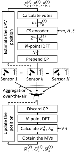
Figure 1: Transmitter and receiver diagrams for the proposed OAC scheme.

IV Performance Analysis

IV-A Average performance

Let $K^{+}_{n}$, $K^{-}_{n}$, and $K^{0}_{n}$ be the number of sensors with positive, negative, and zero votes for $n$th MV computation, respectively.

Lemma 1.

$\mathbb{E}\left[E^{+}_{n}\right]$ and $\mathbb{E}\left[E^{-}_{n}\right]$ can be calculated as

$$\mathbb{E}\left[E^{+}_{n}\right] =\frac{2^{m}{\rm e}^{2\xi}K^{+}_{n}}{1+{\rm e}^{2\xi}}+\frac{2^{m}{\rm e}^{-2\xi}K^{-}_{n}}{1+{\rm e}^{-2\xi}}+{2^{m-1}}(K^{0}_{n}+\sigma_{\rm noise}^{2}),$$

$$\mathbb{E}\left[E^{-}_{n}\right] =\frac{2^{m}K^{+}_{n}}{1+{\rm e}^{2\xi}}+\frac{2^{m}K^{-}_{n}}{1+{\rm e}^{-2\xi}}+{2^{m-1}}(K^{0}_{n}+\sigma_{\rm noise}^{2}),$$

respectively, where the expectation is over the distribution of channel and noise.

The proof is given in Appendix A.

Without any concern about the norm of $\textit{{t}}_{k}^{(\ell)}$ with (10), we can choose an arbitrarily large $\xi$, leading to the following result:

Corollary 1.

The following identities hold:

$$\lim_{\xi\rightarrow\infty}\mathbb{E}\left[E^{+}_{n}\right] =2^{m}K^{+}_{n}+2^{m-1}K^{0}_{n}+2^{m-1}\sigma_{\rm noise}^{2}~{},$$

$$\lim_{\xi\rightarrow\infty}\mathbb{E}\left[E^{-}_{n}\right] =2^{m}K^{-}_{n}+2^{m-1}K^{0}_{n}+2^{m-1}\sigma_{\rm noise}^{2}~{}.$$

Based on Corollary 1, we can infer that the detector in (14) is likely to detect the correct MV for $\xi\rightarrow\infty$ since $\lim_{\xi\rightarrow\infty}\mathbb{E}\left[{E^{+}_{n}-E^{-}_{n}}\right]=2^{m-1}(K^{+}_{n}-K^{-}_{n})$ holds. Also, the impact of absentee votes on the metrics $E^{+}_{n}$ and $E^{-}_{n}$ are equally shared.

IV-B Computation error rate

For a given set of all votes $\textit{{{V}}}^{(\ell)}\triangleq({\textit{{v}}}_{1}^{(\ell)},\hbox to10.00002pt{.\hss.\hss.},{\textit{{v}}}_{K}^{(\ell)})$, the CER can be defined as

$${\tt{CER}}(\textit{{{V}}}^{(\ell)})\triangleq \begin{cases}\mathrm{Pr}({E^{+}_{n}-E^{-}_{n}<0;\textit{{{V}}}^{(\ell)}})~{},&K^{+}_{n}>K^{-}_{n}\\ \mathrm{Pr}({E^{+}_{n}-E^{-}_{n}>0;\textit{{{V}}}^{(\ell)}})~{},&K^{+}_{n}<K^{-}_{n}\\ 1~{},&K^{+}_{n}=K^{-}_{n}\end{cases}~{},$$

$$= \begin{cases}F_{E^{+}_{n}-E^{-}_{n}}\left({x;\textit{{{V}}}^{(\ell)}}\right)~{},&K^{+}_{n}>K^{-}_{n}\\ 1-F_{E^{+}_{n}-E^{-}_{n}}\left({x;\textit{{{V}}}^{(\ell)}}\right)~{},&K^{+}_{n}<K^{-}_{n}\\ 1~{},&K^{+}_{n}=K^{-}_{n}\end{cases}~{},$$ (15)

where $F_{E^{+}_{n}-E^{-}_{n}}\left({x;\textit{{{V}}}^{(\ell)}}\right)$ is the cumulative distribution function (CDF) of $E^{+}_{n}-E^{-}_{n}$. It is worth noting that the detector in (14) always makes an error due to the noisy reception in communication channels when $K^{+}_{n}$ and $K^{-}_{n}$ are identical to each other, leading to the third case in (15). For a given $\textit{{{V}}}^{(\ell)}$, the CDF of $E^{+}_{n}-E^{-}_{n}$ can be obtained as follows:

Lemma 2.

Suppose $h_{k,{i}}\sim\mathcal{CN}({0,1})$ (i.e., frequency-selective fading) holds. $F_{E^{+}_{n}-E^{-}_{n}}\left({x;\textit{{{V}}}^{(\ell)}}\right)$ can be calculated as

$$F_{E^{+}_{n}-E^{-}_{n}}\left({x;\textit{{{V}}}^{(\ell)}}\right) =\frac{1}{2}-\int_{-\infty}^{\infty}\frac{\varphi^{+}_{n}(t){{\varphi}^{-}_{n}(t)}^{*}}{2\pi{\rm j}t}dt~{},$$ (16)

respectively, where $\varphi^{+}_{n}(t)$ and $\varphi^{-}_{n}(t)$ are given by

$$\varphi^{+}_{n}(t)\triangleq\prod_{{\begin{subarray}{c}\forall\textit{{x}}\in\mathbb{Z}^{m}_{2}\\ y_{{\pi_{n}}}=1\end{subarray}}}\frac{1}{1-{\rm j}t\lambda_{{i}(\textit{{x}})}^{-1}}~{},$$ (17)

and

$$\varphi^{-}_{n}(t)\triangleq\prod_{{\begin{subarray}{c}\forall\textit{{x}}\in\mathbb{Z}^{m}_{2}\\ y_{{\pi_{n}}}=0\end{subarray}}}\frac{1}{1-{\rm j}t\lambda_{{i}(\textit{{x}})}^{-1}},$$ (18)

respectively, for $\lambda_{{i}(\textit{{x}})}^{-1}\triangleq\sum_{k=1}^{K}{\rm e}^{2f_{{\rm r},k}(\textit{{x}})}+\sigma_{\rm noise}^{2}$.

The proof is given in Appendix B.

Although $F_{E^{+}_{n}-E^{-}_{n}}\left({x;\textit{{{V}}}^{(\ell)}}\right)$ in (16) is not a closed-form expression, it can be easily evaluated with a numeric integration to compute ${\tt{CER}}(\textit{{{V}}}^{(\ell)})$ in (15). Also, as demonstrated in Section VI (i.e., Figure 3), (16) holds approximately in the flat-fading channel since the values for $b_{k,0}^{(\ell)},b_{k,1}^{(\ell)},\hbox to10.00002pt{.\hss.\hss.},b_{k,m}^{(\ell)}$ are chosen randomly in our approach.

Let $\alpha$, $\beta$, and $\gamma$ denote the probabilities given by $\mathrm{Pr}({v_{k,n}^{(\ell)}>0})$, $\mathrm{Pr}({v_{k,n}^{(\ell)}<0})$, and $\mathrm{Pr}({v_{k,n}^{(\ell)}=0})$, respectively, $\forall k\in\{1,\hbox to10.00002pt{.\hss.\hss.},K\}$ and $\forall n\in\{1,\hbox to10.00002pt{.\hss.\hss.},m\}$.

Corollary 2.

For given ${\textit{{v}}}_{n}^{(\ell)}={({{\mathbf{1}}}_{K^{+}_{n}},{{{\mathbf{0}}}}_{K^{0}_{n}},-{{\mathbf{1}}}_{K^{-}_{n}})}$, $\alpha$, $\beta$, and $\gamma$, the CER for the $n$th MV is given by

$${\tt{CER}}(n;{K^{+}_{n},K^{-}_{n},K^{0}_{n}})$$

$$~{}~{}~{}~{}~{}~{}=\begin{cases}{\tt{CER}^{+}}(n;{K^{+}_{n},K^{-}_{n},K^{0}_{n}})~{},&K^{+}_{n}>K^{-}_{n}\\ {\tt{CER}^{-}}(n;{K^{+}_{n},K^{-}_{n},K^{0}_{n}})~{},&K^{+}_{n}<K^{-}_{n}\\ 1~{},&K^{+}_{n}=K^{-}_{n}\end{cases}~{},$$ (19)

where

$${\tt{CER}^{+}}(n;{K^{+}_{n},K^{-}_{n},K^{0}_{n}})$$

$$~{}~{}\triangleq\frac{1}{2}-\sum_{\forall\dot{\textit{{{V}}}}}\alpha^{N^{+}}\beta^{N^{-}}\gamma^{N^{0}}\int_{-\infty}^{\infty}\frac{\varphi^{+}_{n}(t){{\varphi}^{-}_{n}(t)}^{*}}{2\pi{\rm j}t}dt~{},$$ (20)

$${\tt{CER}^{-}}(n;{K^{+}_{n},K^{-}_{n},K^{0}_{n}})$$

$$~{}~{}\triangleq\frac{1}{2}+\sum_{\forall\dot{\textit{{{V}}}}}\alpha^{N^{+}}\beta^{N^{-}}\gamma^{N^{0}}\int_{-\infty}^{\infty}\frac{\varphi^{+}_{n}(t){{\varphi}^{-}_{n}(t)}^{*}}{2\pi{\rm j}t}dt~{},$$ (21)

respectively, where ${N^{+}}$, ${N^{-}}$, and ${N^{0}}$ are the number of elements in $\dot{\textit{{{V}}}}\triangleq({\textit{{v}}}_{1}^{(\ell)},\hbox to10.00002pt{.\hss.\hss.},{\textit{{v}}}_{n-1}^{(\ell)},{\textit{{v}}}_{n+1}^{(\ell)},\hbox to10.00002pt{.\hss.\hss.},{\textit{{v}}}_{K}^{(\ell)})$ with $1$, $-1$, and $0$, respectively.

Proof.

The probability of a realization of $\dot{\textit{{{V}}}}$ is $\alpha^{N^{+}}\beta^{N^{-}}\gamma^{N^{0}}$. Thus, the expectation of (15) over the distribution of $\dot{\textit{{{V}}}}$ leads to (20) and (21). ∎

The calculations of (20) and (21) can be intractable due to the enumerations of $\dot{\textit{{{V}}}}$. To address this issue, we average the CER in (15) over a few realizations of $\textit{{{V}}}^{(\ell)}$ for a given triplet $\{\alpha,\beta,\gamma\}$ to compute (20) and (21) in Section VI.

Finally, let us define ${\tt{CER}}$ by setting it as

$${\tt{CER}}=\mathrm{Pr}({\hat{w}_{n}^{(\ell)}\neq w_{n}^{(\ell)}})~{},$$ (22)

for given $\alpha$, $\beta$, and $\gamma$. We can calculate ${\tt{CER}}$ as follows:

Corollary 3.

For given $\alpha$, $\beta$, and $\gamma$, ${\tt{CER}}$ is given by

$${\tt{CER}} =\mathrm{Pr}({\hat{w}_{n}^{(\ell)}=-1,w_{n}^{(\ell)}=1})+\mathrm{Pr}({\hat{w}_{n}^{(\ell)}=1,w_{n}^{(\ell)}=-1})$$

$$~{}~{}~{}+\mathrm{Pr}({w_{n}^{(\ell)}=0})~{},$$ (23)

where

$$\mathrm{Pr}({\hat{w}_{n}^{(\ell)}=-1,w_{n}^{(\ell)}=1})$$

$$=\sum_{l=0}^{K}\sum_{k=l+1}^{K-l}\binom{K}{k}\binom{K-k}{l}\alpha^{k}\beta^{l}\gamma^{K-k-l}{\tt{CER}^{+}}(n;{k,l,m})~{},$$

$$\mathrm{Pr}({\hat{w}_{n}^{(\ell)}=1,w_{n}^{(\ell)}=-1})$$

$$=\sum_{k=0}^{K}\sum_{l=k+1}^{K-k}\binom{K}{k}\binom{K-k}{l}\alpha^{k}\beta^{l}\gamma^{K-k-l}{\tt{CER}^{-}}(n;{k,l,m})~{},$$

$$\mathrm{Pr}({w_{n}^{(\ell)}=0})=\sum_{k=0}^{\lfloor\frac{K}{2}\rfloor}\binom{K}{k}\binom{K-k}{k}\alpha^{k}\beta^{k}\gamma^{K-2k}~{}.$$

The third term in (23) is because of the third case in (19). In Section VI, we evaluate ${\tt{CER}}$ for different $\alpha$, $\beta$, and $\gamma$ values.

IV-C Computation rate and resource utilization ratio

The computation rate $\mathcal{R}$ can be defined as the number of functions computed per channel use (in real dimension) [8, 36]. Since the proposed scheme computes $m$ MVs over $2^{m}$ complex-valued resources, $\mathcal{R}$ can be expressed as

$$\mathcal{R}=\frac{m}{2^{m+1}}~{}.$$ (24)

Hence, for a larger $m$, the computation rate reduces, while the CER improves significantly as demonstrated in Section VI.

Let us define the resource utilization ratio as the ratio between the number of resources consumed with the proposed scheme and the number of resources when the communication and computation are considered as separate tasks, i.e., the traditional first-communicate-then-compute approach. For the separation, we assume that the spectral efficiency is $r$ bit/s/Hz. Hence, the total number of resources needed for $K$ EDs and $m$ bits (i.e., votes) can be obtained as $rmK$. The proposed scheme consumes $2^{m}$ complex-valued resources for $K$ EDs. Hence, the resource utilization ratio can be expressed as

$$\epsilon=\frac{2^{m}}{rmK}~{}.$$ (25)

For instance, for $r=1$, $m=7$, and $K=50$, the wireless resources needed with the proposed scheme is $\epsilon=0.3657$ times the ones with the traditional approach.

V Convergence Analysis

In this section, we discuss the convergence of the resulting systems under the control strategies in (3) by analyzing their Lyapunov stability based on the following definition:

Definition 1 ([37]).

A stochastic system $x^{(\ell+1)}=f\left(x^{(\ell)}\right)$, where $f$ describes the dynamics and $x^{(\ell)}$ is the state, is called globally uniformly ultimately bounded in mean square with ultimate bound $b$, if there exist positive $b$ and $L$ such that for any $\mathbb{E}\left[\|x^{(0)}\|^{2}\right]<\infty$, the inequality $\mathbb{E}\left[\|x^{(\ell)}\|^{2}\right]\leq b$ holds for all $\ell\geq L$.

We define $\delta^{(\ell)}_{l}$ by setting $\delta^{(\ell)}_{l}={{c}}^{({\ell})}_{l}-{c}_{\mathrm{t},l}$ and re-express (1) as

$$\delta^{(\ell+1)}_{l}=\delta^{(\ell)}_{l}-T_{\mathrm{update}}{u}^{(\ell)}_{l}.$$ (26)

for the convergence analysis of each case in (3).

V-A Case 1: Continuous update & ideal communications

The control strategy can be written as

$${g}^{(\ell)}_{l} =\frac{1}{K}\sum_{k=1}^{K}\left({{c}}^{({\ell})}_{l}+{\epsilon}^{(\ell)}_{k,l}-{c}_{\mathrm{t},l}\right)=\delta^{(\ell)}_{l}+\frac{1}{K}\sum_{k=1}^{K}{\epsilon}^{(\ell)}_{k,l}~{}.$$

Since ${\epsilon}^{(\ell)}_{k,l}$ is Gaussian and the summands are independent of each other, $\frac{1}{K}\sum_{k=1}^{K}{\epsilon}^{(\ell)}_{k,l}$ is also Gaussian. Based on stochastic control theory [38], as long as $|1-\mu T_{\mathrm{update}}|<1$, the resulting closed-loop system is stable in a stochastic sense.

V-B Case 2: MV-based update & ideal communications

In this case, $|{g}^{(\ell)}_{l}|$ is at most 1. Therefore, as long as $\mu\leq u_{\text{\rm limit}}$, input saturation will not happen and the dynamic can be written as

$$\delta^{(\ell+1)}_{l} =\delta^{(\ell)}_{l}-\mu T_{\mathrm{update}}\>{\rm\operatorname{sign}}\left(\sum_{k=1}^{K}\bar{c}_{k,l}^{(\ell)}\right)$$ (27)

$$=\delta^{(\ell)}_{l}-\mu T_{\mathrm{update}}\>{g}^{(\ell)}_{l}.$$

Recall that $\bar{c}_{k,l}^{(\ell)}=\text{sign}\left({{\tilde{c}}}^{({\ell})}_{k,l}-{c}_{\mathrm{t},l}\right)={\rm sign}\left(\delta^{(\ell)}_{l}+{\epsilon}^{(\ell)}_{k,l}\right)$ and ${\epsilon}^{(\ell)}_{k,l}$ is Gaussian. We can then obtain the values of $\alpha$, $\beta$, and $\gamma$ as

$$\alpha ={\rm Pr}(\bar{c}_{k,l}^{(\ell)}=+1)={\rm Pr}(\delta^{(\ell)}_{l}+{\epsilon}^{(\ell)}_{k,l}>0)$$

$$={\rm Pr}\left(\frac{{\epsilon}^{(\ell)}_{k,l}}{\sigma_{\rm s}}>\frac{-\delta^{(\ell)}_{l}}{\sigma_{\rm s}}\right)=1-\Phi\left(\frac{-\delta^{(\ell)}_{l}}{\sigma_{\rm s}}\right)~{},$$ (28)

$$\beta ={\rm Pr}(\bar{c}_{k,l}^{(\ell)}=-1)={\rm Pr}(\delta^{(\ell)}_{l}+{\epsilon}^{(\ell)}_{k,l}<0)$$

$$={\rm Pr}\left(\frac{{\epsilon}^{(\ell)}_{k,l}}{\sigma_{\rm s}}<\frac{-\delta^{(\ell)}_{l}}{\sigma_{\rm s}}\right)=\Phi\left(\frac{-\delta^{(\ell)}_{l}}{\sigma_{\rm s}}\right)~{},$$ (29)

$$\gamma ={\rm Pr}(\bar{c}_{k,l}^{(\ell)}=0)=0~{},$$

respectively. With the distribution of $\bar{c}_{k,l}^{(\ell)}$, we have

$$\phi_{+}({\delta^{(\ell)}_{l}}) \triangleq{\rm Pr}\left({g}^{(\ell)}_{l}=+1\right)=\sum_{k=0}^{\lceil\frac{K}{2}\rceil-1}\binom{K}{k}\alpha^{K-k}\beta^{k}~{},$$ (30)

$$\phi_{-}({\delta^{(\ell)}_{l}}) \triangleq{\rm Pr}\left({g}^{(\ell)}_{l}=-1\right)=\sum_{k=0}^{\lceil\frac{K}{2}\rceil-1}\binom{K}{k}\alpha^{k}\beta^{K-k}~{},$$ (31)

$$\phi_{0}({\delta^{(\ell)}_{l}}) \triangleq\begin{cases}0,&{\rm odd~{}}K\\ \binom{K}{{K}/{2}}\alpha^{\frac{K}{2}}\beta^{\frac{K}{2}},&{\rm even~{}}K\end{cases}.$$ (32)

Given the distribution of ${g}^{(\ell)}_{l}$, we can show the convergence of the system under the MV (ideal) case:

Theorem 2.

Given $\mu\leq u_{\text{\rm limit}}$, the system in (26) is globally uniformly ultimately bounded in mean square under the MV (ideal) control strategy in (3).

Proof.

Let $V\left(x\right)\triangleq x^{2}$. Then, by using (27),

$$\mathbb{E}\left[V\left(\delta^{(\ell+1)}_{l}\right)|\delta^{(\ell)}_{l}\right]-V\left(\delta^{(\ell)}_{l}\right)$$ (33)

$$=-2\mu T_{\mathrm{update}}\mathbb{E}\left[{g}^{(\ell)}_{l}|\delta^{(\ell)}_{l}\right]\delta^{(\ell)}_{l}+\mu^{2}T_{\mathrm{update}}^{2}\mathbb{E}\left[({g}^{(\ell)}_{l})^{2}|\delta^{(\ell)}_{l}\right].$$

By using (30) and (31),

$$\mathbb{E}\left[{g}^{(\ell)}_{l}|\delta^{(\ell)}_{l}\right]=\phi_{+}({\delta^{(\ell)}_{l}})-\phi_{-}({\delta^{(\ell)}_{l}})~{},$$ (34)

$$\mathbb{E}\left[({g}^{(\ell)}_{l})^{2}|~{}\delta^{(\ell)}_{l}\right]=\phi_{+}({\delta^{(\ell)}_{l}})+\phi_{-}({\delta^{(\ell)}_{l}})\in[0,1]~{}.$$ (35)

Therefore, by using (34) and (35), (33) yields

$$\mathbb{E}\left[V\left(\delta^{(\ell+1)}_{l}\right)|\delta^{(\ell)}_{l}\right]-V\left(\delta^{(\ell)}_{l}\right)$$

$$=-2\mu T_{\mathrm{update}}\left(\phi_{+}({\delta^{(\ell)}_{l}})-\phi_{-}({\delta^{(\ell)}_{l}})\right)\delta^{(\ell)}_{l}$$

$$~{}~{}~{}~{}+\mu^{2}T_{\mathrm{update}}^{2}\left(\phi_{+}({\delta^{(\ell)}_{l}})+\phi_{-}({\delta^{(\ell)}_{l}})\right)$$

$$\leq-2\mu T_{\mathrm{update}}\left(\phi_{+}({\delta^{(\ell)}_{l}})-\phi_{-}({\delta^{(\ell)}_{l}})\right)\delta^{(\ell)}_{l}+\mu^{2}T_{\mathrm{update}}^{2}~{}.$$

Note that $\delta^{(\ell)}_{l}>0\Rightarrow\phi_{+}({\delta^{(\ell)}_{l}})>\phi_{-}({\delta^{(\ell)}_{l}})$ and $\delta^{(\ell)}_{l}<0\Rightarrow\phi_{+}({\delta^{(\ell)}_{l}})<\phi_{-}({\delta^{(\ell)}_{l}})$, which means

$$\left(\phi_{+}({\delta^{(\ell)}_{l}})-\phi_{-}({\delta^{(\ell)}_{l}})\right)\delta^{(\ell)}_{l}>0~{},$$

always holds. Meanwhile, $\left(\phi_{+}({\delta^{(\ell)}_{l}})-\phi_{-}({\delta^{(\ell)}_{l}})\right)\delta^{(\ell)}_{l}$ is monotonic increasing when $\delta^{(\ell)}_{l}>0$ and monotonic decreasing when $\delta^{(\ell)}_{l}<0$ with the global minimum at $\delta^{(\ell)}_{l}=0$. Thus, we can define

$$\gamma=\max_{q\in\mathbb{R}}|q|,~{}~{}{\rm s.t.}~{}~{}\left(\phi_{+}({q})-\phi_{-}({q})\right)q=\frac{\mu T_{\mathrm{update}}}{2}~{},$$

and the parameter $\gamma$ must be finite, whose value depends on $\mu T_{\mathrm{update}}$ and $\sigma_{\rm s}$. For any $\delta^{(\ell)}_{l}$ such that $|\delta^{(\ell)}_{l}|>\gamma$, we have

$$\left(\phi_{+}({\delta^{(\ell)}_{l}})-\phi_{-}({\delta^{(\ell)}_{l}})\right)\delta^{(\ell)}_{l}>\frac{\mu T_{\mathrm{update}}}{2}~{},$$

and then

$$\mathbb{E}\left[V\left(\delta^{(\ell+1)}_{l}\right)|\delta^{(\ell)}_{l}\right]-V\left(\delta^{(\ell)}_{l}\right)<0~{}.$$

Thus, the system is mean-square globally uniformly ultimately bounded and the mean-square ultimate bound is determined by $\gamma$. ∎

V-C Case 3: MV with the proposed OAC

By using Corollary 2, we can re-calculate $\phi_{+}({\delta^{(\ell)}_{l}})$ and $\phi_{-}({\delta^{(\ell)}_{l}})$ defined in (30) and (31), respectively, as

$$\phi_{+}({\delta^{(\ell)}_{l}})=1-\underbrace{\sum_{k=0}^{K}\binom{K}{k}\alpha^{k}\beta^{K-k}{\tt{CER}^{+}}(n;{k,K-k,0})}_{\triangleq\zeta}~{},$$

$$\phi_{-}({\delta^{(\ell)}_{l}})=1-\phi_{+}({\delta^{(\ell)}_{l}})~{},$$

where $\alpha$ and $\beta$ are given in (28) and (29), respectively. Now the convergence of the system under the OAC (MV) strategy is presented in the following theorem:

Theorem 3.

Given $\mu\leq u_{\text{\rm limit}}$, the system in (26) is globally uniformly ultimately bounded in mean square under the MV (OAC) control strategy in (14).

Proof.

Similar to the proof of Theorem 2, let $V\left(x\right)\triangleq x^{2}$ and we have

$$\mathbb{E}\left[V\left(\delta^{(\ell+1)}_{l}\right)|\delta^{(\ell)}_{l}\right]-V\left(\delta^{(\ell)}_{l}\right)$$

$$=-2\mu T_{\mathrm{update}}\>\mathbb{E}\left[{g}^{(\ell)}_{l}|\delta^{(\ell)}_{l}\right]\delta^{(\ell)}_{l}+\mu^{2}T_{\mathrm{update}}^{2}\mathbb{E}\left[({g}^{(\ell)}_{l})^{2}|~{}\delta^{(\ell)}_{l}\right].$$

Based on the distribution of ${g}^{(\ell)}_{l}$ for the OAC (MV) case,

$$\mathbb{E}\left[{g}^{(\ell)}_{l}|\delta^{(\ell)}_{l}\right]=\phi_{+}({\delta^{(\ell)}_{l}})-\phi_{-}({\delta^{(\ell)}_{l}})=1-2\zeta~{},$$

$$\mathbb{E}\left[({g}^{(\ell)}_{l})^{2}|~{}\delta^{(\ell)}_{l}\right]=1~{}.$$

Therefore,

$$\mathbb{E}\left[V\left(\delta^{(\ell+1)}_{l}\right)|\delta^{(\ell)}_{l}\right]-V\left(\delta^{(\ell)}_{l}\right)$$

$$=-2\mu T_{\mathrm{update}}\>\left(\phi_{+}({\delta^{(\ell)}_{l}})-\phi_{-}({\delta^{(\ell)}_{l}})\right)\delta^{(\ell)}_{l}+\mu^{2}T_{\mathrm{update}}^{2}~{}.$$

Note that $\zeta<1/2$ for $\delta^{(\ell)}_{l}>0$ and $\zeta>1/2$ for $\delta^{(\ell)}_{l}<0$ with the proposed OAC scheme, which means

$$\left(\phi_{+}({\delta^{(\ell)}_{l}})-\phi_{-}({\delta^{(\ell)}_{l}})\right)\delta^{(\ell)}_{l}>0~{},$$

always holds. Thus, following a similar analysis in the proof of Theorem 2, we conclude that the system is mean-square globally uniformly ultimately bounded and the ultimate bound is determined by $\mu T_{\mathrm{update}}$ and $\sigma_{\rm s}$. ∎

VI Numerical Results

In this section, we first numerically analyze the performance of the scheme for an arbitrary application. Subsequently, we apply it to the UAV waypoint flight control scenario discussed in Section II. For all analyses, we assume that there are $K=50$ sensors. For comparison, we also generate our results with Goldenbaum’s non-coherent OAC scheme discussed in [28]. In this approach, the power of the transmitted signal is modulated. To this end, a transmitter maps three possible votes, i.e., $-1$, $0$, and $1$, to the symbols $0$, $1$, and $2$, respectively, and multiplies a unimodular random sequence of length $L$ with the square of the symbol to be aggregated. The receiver calculates the norm-square of the aggregated sequences and re-scales it with $f(x)=x/L-K$. It then calculates the sign of scaled value to obtain the MV. To make a fair comparison, $L$ is set to the nearest integer to $2^{m}/m$, and $m$ sequences are mapped to the subcarriers back-to-back to compute $m$ MVs. We choose the phase of an element of unimodular sequence uniformly between 0 and $2\pi$.

VI-A CER and PMEPR results

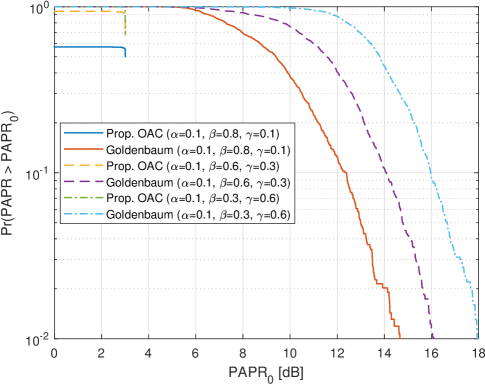
Figure 2: PMEPR distribution.

In Figure 2, we analyze the PMEPR distribution of the transmitted signals for $m=8$, $L=32$, $\alpha=0.1$, and $\gamma\in\{0.1,0.3,0.6\}$. As can be seen from Figure 2, the PMEPR of a transmitted signal with the proposed scheme is always less than or equal to $3$ dB due to the properties of the CSs. If there are no absentee votes, the maximum PMEPR of the proposed scheme is $0$ dB since a single subcarrier is used for the transmission (see the cases for ${\textit{{v}}}_{k}^{(\ell)}=(1,1,1)$ and ${\textit{{v}}}_{k}^{(\ell)}=(1,1,-1)$ in Example 1). Hence, for a larger absentee vote probability, the probability of observing $0$ dB PMEPR increases. The combination of sequences that lead to $0$ dB and $3$ dB PMEPR values and results in the jumps in the PMEPR distribution given in Figure 2. The PMEPR characteristics for Goldenbaum’s approach are similar to the ones for typical OFDM transmissions and the gap between the proposed scheme and Goldenbaum’s approach is considerable large in term of PMEPR.

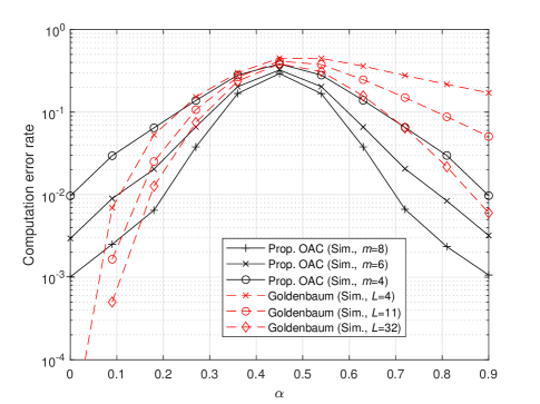
(a) CER in flat-fading channel ($\gamma=0.1$).

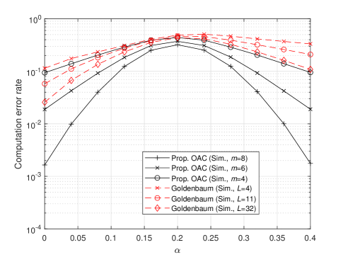
(b) CER in flat-fading channel ($\gamma=0.6$).

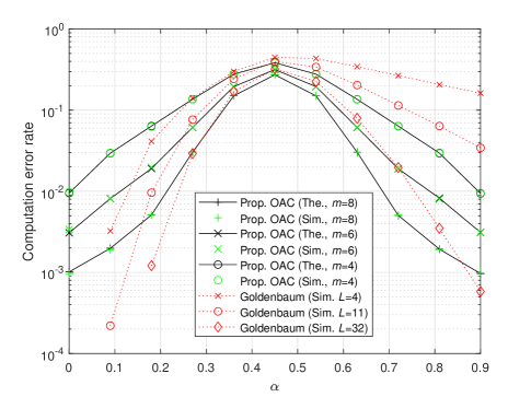
(c) CER in frequency-selective channel ($\gamma=0.1$).

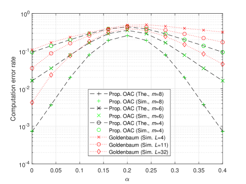
(d) CER in frequency-selective channel ($\gamma=0.6$).

Figure 3: CER for in AWGN, flat-fading, and frequency-selective channels ($K=50$ sensors).

In Figure 3, we analyze ${\tt{CER}}$ defined in (22) for $\gamma\in\{0.1,0.6\}$, $m=\{4,6,8\}$ for the proposed scheme and $L=\{4,11,32\}$ for Goldenbaum’s approach by sweeping $\alpha$ in flat-fading (i.e., $h_{k,{i}}=h_{k,{i}^{\prime}}\sim\mathcal{CN}({0,1})$, ${i}\neq{i}^{\prime}$) and frequency-selective (i.e., $h_{k,{i}}\sim\mathcal{CN}({0,1})$) channels, respectively. For both schemes, as expected, the CER improves for a small or a large $\alpha$ since more sensors vote for $-1$ or $+1$, respectively. The performance in the frequency selective channel is slightly better than the flat-fading channel because of the diversity gain. Also, both schemes achieve a better CER for increasing $m$ or $L$ at the expense of more resource consumption in all channel conditions. On the other hand, while the proposed scheme exhibits a balanced behavior, the Goldenbaum’s approach tends to perform better for a smaller $\alpha$ as the transmitters do not transmit for vote $-1$. For $\gamma=0.1$, the proposed scheme performs better than Goldenbaum’s approach for $\alpha\in[0.27,0.8]$. When there are more absentee votes, i.e., $\gamma=0.6$, the proposed scheme is superior to Goldenbaum’s scheme for all values of $\alpha$, as can be seen in Figure 3LABEL:sub@subfig:CER01selectiveFading and Figure 3LABEL:sub@subfig:CER06selectiveFading. Also, the theoretical CERs based on the expression in (23) are well-aligned with the simulation results in Figure 3LABEL:sub@subfig:CER01selectiveFading and Figure 3LABEL:sub@subfig:CER06selectiveFading.

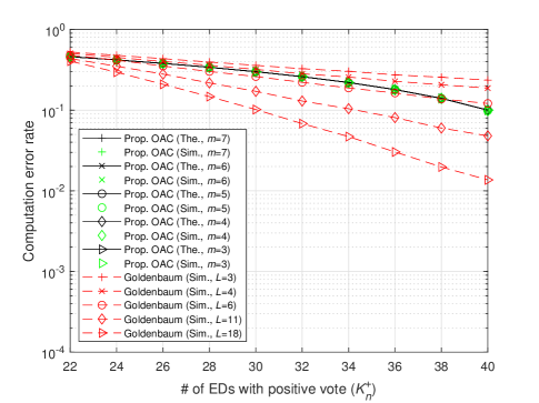
(a) $\alpha=1$, $\beta=0$, $\gamma=0$ or $\alpha=0$, $\beta=1$, $\gamma=0$.

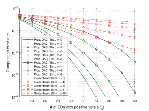
(b) $\alpha=1/2$, $\beta=1/2$, $\gamma=0$.

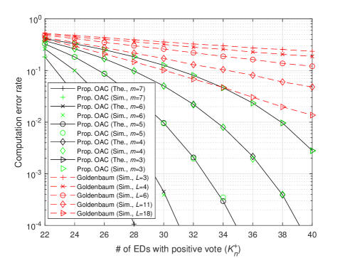
(c) $\alpha=0$, $\beta=0$, $\gamma=1$.

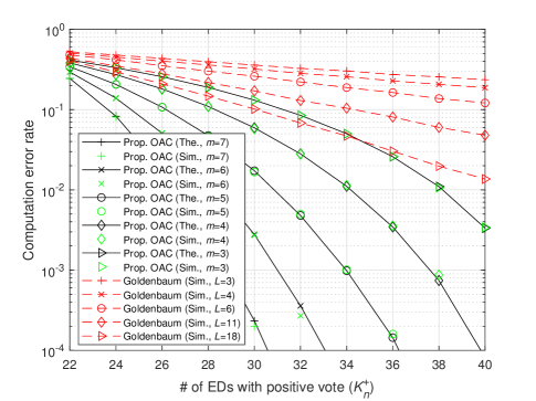
(d) $\alpha=1/3$, $\beta=1/3$, $\gamma=1/3$.

Figure 4: ${\tt{CER}^{+}}(n;{K^{+}_{n},K^{-}_{n},K^{0}_{n}})$ for different values of $\alpha$, $\beta$, $\gamma$ ($K=50$ EDs, $K^{0}_{n}=10$ EDs, ${\tt{SNR}}=10$ dB, frequency-selective fading channel).

In Figure 4, we evaluate ${\tt{CER}}(n;{K^{+}_{n},K^{-}_{n},K^{0}_{n}})$ in Corollary 2 in frequency-selective fading channel by increasing $K^{+}_{n}$ from $22$ to $40$ for $K^{0}_{n}=10$ (i.e., the first case of (19)), ${\tt{SNR}}=10$ dB, $m\in\{3,4,5,6,7\}$ for the proposed scheme and $L\in\{3,4,6,11,18\}$ for the Goldenbaum’s approach. In Figure 4LABEL:sub@subfig:case_p1_p0_z0_errProb, we assume $\alpha=1$, $\beta=0$, and $\gamma=0$ (or $\alpha=0$, $\beta=1$, and $\gamma=0$). As $\gamma=0$, there are no absentee votes. Also, the same number of sensors activates the same element of the transmitted sequence for all realizations. Since the other elements are not used for the transmission and the energy accumulation is non-coherent, the scheme does not provide any performance gain with increasing $m$. In Figure 4LABEL:sub@subfig:case_p12_p12_z0_errProb, we assume that $\alpha=1/2$, $\beta=1/2$, and $\gamma=0$. As compared to the previous case, we observe a significant improvement with increasing $m$. This is because the randomness enables the votes to accumulate on $2^{m-1}$ subcarriers, rather than a single resource. Hence, accumulating the energy over multiple subcarriers yields a better estimation of $E^{+}_{n}$ and $E^{-}_{n}$. A similar result is given in Figure 4LABEL:sub@subfig:case_p0_p0_z1_errProb when all the sensors have absentee votes, i.e., $\alpha=0$, $\beta=0$, and $\gamma=1$. This is due to the fact that all sensors activate $2^{m-1}$ elements of the transmitted CS. Hence, the CER decreases when $m$ increases. Finally, in Figure 4LABEL:sub@subfig:case_p13_p13_z13_errProb, we analyze the case for $\alpha=1/3$, $\beta=1/3$, and $\gamma=1/3$ and show that CER performance improves increasing $m$. For all cases, the theoretical results exactly match with the simulations and the CER performance improves with increasing $K^{+}_{n}$. For Goldenbaum’s scheme, each MV is calculated on orthogonal resources. Hence, the corresponding ${\tt{CER}}(n;{K^{+}_{n},K^{-}_{n},K^{0}_{n}})$ is not a function of $\alpha$, $\beta$, and $\gamma$. We observe that Goldenbaum’s scheme performs better for a larger $L$. However, since the proposed scheme can exploit the available number of subcarriers much more effectively, it yields notably better performance, as can be seen in Figure 4LABEL:sub@subfig:case_p12_p12_z0_errProb-LABEL:sub@subfig:case_p13_p13_z13_errProb.

VI-B UAV waypoint flight control

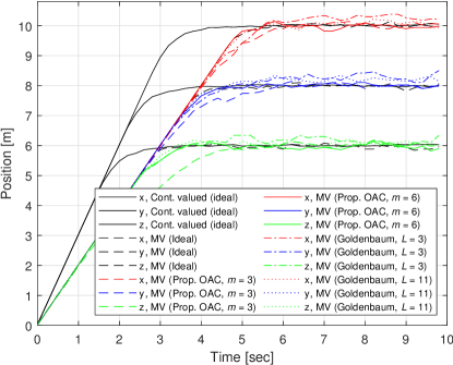
(a) UAV’s trajectory in time.

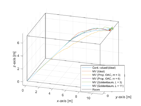
(b) UAV’s trajectory in space.

Figure 5: UAV’s trajectory with a single point of interest. The initial position is $(0,0,0)$ and the target position is $(10,8,6)$.

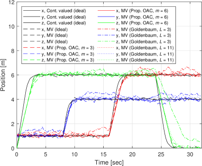
(a) UAV’s trajectory in time.

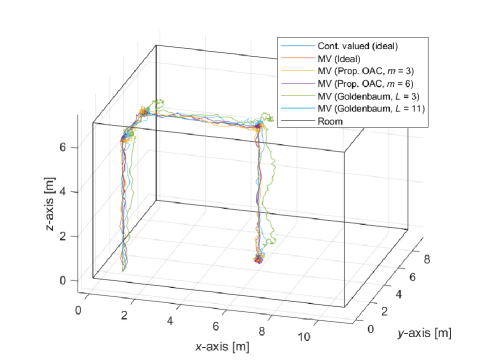
(b) UAV’s trajectory in space.

Figure 6: UAV’s trajectory with multiple points of interest, i.e., $(1,1,6)$, $(1,4,6)$, $(6,4,6)$, and $(6,4,0)$. The initial position is $(1,1,0)$.

In Figure 5 and Figure 6, we consider the UAV waypoint flight control scenario discussed in Section II for $K=50$ sensors. We assume $T_{\mathrm{update}}=10$ ms, $\mu=2$, $u_{\text{\rm limit}}=3$ m/s, $\sigma_{\rm s}^{2}=2$, and ${\tt{SNR}}=10$ dB. We provide the trajectory of the UAV in time and space. We consider two cases. In the first case, there is only one point of interest $({c}_{\mathrm{t},1},{c}_{\mathrm{t},2},{c}_{\mathrm{t},3})=(10,8,6)$ and the initial position of the UAV is $(0,0,0)$. In the second case, the points of interest are $(1,1,6)$, $(1,4,6)$, $(6,4,6)$, and $(6,4,0)$, where the initial position of the UAV is $(1,1,0)$. We compare the proposed scheme for $m\in\{3,6\}$ with both continuous and MV-based feedback in an ideal communication channel (i.e., no error due to the communication) and Goldenbaum’s approach for $L\in\{3,11\}$. As can be seen from Figure 5LABEL:sub@subfig:wayPointSingleTime, for the continuous-valued feedback, the UAV reaches its position faster than any MV-based approach. This is because the velocity increment is limited by the step size for MV-based feedback in our setup. Hence, as can be seen from Figure 5LABEL:sub@subfig:wayPointSingleSpace the UAV’s trajectory in space is slightly bent. Since the proposed scheme is also based on the MV computation, its characteristics are similar to the one with MV computation in an ideal channel. Since the CER with $m=6$ is lower than the one with $m=3$, the proposed scheme for $m=6$ performs better and its characteristics are similar to the ideal MV-based feedback. Goldebaum’s approach has similar characteristics to the proposed scheme in terms of trajectory. However, the variation of the UAV position is considerably large when the UAV reaches its final point, as can be seen in Figure 5LABEL:sub@subfig:wayPointSingleSpace, in particular for $L=3$. The position of the UAV in time and space for multiple points of interest is given in Figure 6LABEL:sub@subfig:wayPointTime and Figure 6LABEL:sub@subfig:waypointSpace, respectively. The proposed scheme for $m=6$ performs similarly to the one with the MVs in ideal communications and increasing $m$ leads to a more stable trajectory. For $L=3$, the trajectory is less stable for Goldenbaum’s method. However, its performance improves for a larger $L$ for Goldenbaum’s approach.

VII Concluding Remarks

In this study, we modulate the amplitude of the CS based on Theorem 1 to develop a new non-coherent OAC scheme for MV computation. We show that the proposed scheme reduces the CER via bandwidth expansion in both flat-fading and frequency-selective fading channel conditions while maintaining the PMEPR of the transmitted signals to be less than or equal to $3$ dB. In this work, we derive the theoretical CER and provide the convergence analyses for a control scenario. We show that the proposed scheme results in a lower CER as compared with Goldenbaum’s method while providing a large PMEPR gain. Finally, we demonstrate its applicability to an indoor flight control scenario. The proposed scheme with a larger length of sequences performs similarly to the case where MV without OAC. The proposed approach can also be utilized in other applications, such as wireless federated learning or distributed optimization over wireless networks using MV computation, to address the congestion problems in band-limited wireless channels.

Appendix A Proof of Lemma 1

We first need the following proposition:

Proposition 1.

The following identities hold:

$$\sum_{\begin{subarray}{c}\forall\textit{{x}}\in\mathbb{Z}^{m}_{2}\\ y_{{\pi_{n}}}=1\end{subarray}}{\rm e}^{2f_{{\rm r},k}(\textit{{x}})}={\rm e}^{2a_{k,n}^{(\ell)}}\sum_{\begin{subarray}{c}\forall\textit{{x}}\in\mathbb{Z}^{m}_{2}\\ y_{{\pi_{n}}}=0\end{subarray}}{\rm e}^{2f_{{\rm r},k}(\textit{{x}})}=\frac{{\rm e}^{2a_{k,n}^{(\ell)}}}{1+{\rm e}^{2a_{k,n}^{(\ell)}}}2^{m}~{}.$$

Proof.

The first identity is because ${\rm e}^{2a_{k,n}^{(\ell)}y_{{\pi_{n}}}}=1$ for $y_{{\pi_{n}}}=0$. Under (10), $\lVert\textit{{t}}_{k}^{(\ell)}\rVert_{2}^{2}=2^{m}$ holds. Hence,

$$\lVert\textit{{t}}_{k}^{(\ell)}\rVert_{2}^{2}= \sum_{\forall\textit{{x}}\in\mathbb{Z}^{m}_{2}}{\rm e}^{2f_{{\rm r},k}(\textit{{x}})}=\sum_{\begin{subarray}{c}\forall\textit{{x}}\in\mathbb{Z}^{m}_{2}\\ y_{{\pi_{n}}}=0\end{subarray}}{\rm e}^{2f_{{\rm r},k}(\textit{{x}})}+\sum_{\begin{subarray}{c}\forall\textit{{x}}\in\mathbb{Z}^{m}_{2}\\ y_{{\pi_{n}}}=1\end{subarray}}{\rm e}^{2f_{{\rm r},k}(\textit{{x}})}$$

$$= \sum_{\begin{subarray}{c}\forall\textit{{x}}\in\mathbb{Z}^{m}_{2}\\ y_{{\pi_{n}}}=0\end{subarray}}{\rm e}^{2f_{{\rm r},k}(\textit{{x}})}+{\rm e}^{2a_{k,n}^{(\ell)}}\sum_{\begin{subarray}{c}\forall\textit{{x}}\in\mathbb{Z}^{m}_{2}\\ y_{{\pi_{n}}}=0\end{subarray}}{\rm e}^{2f_{{\rm r},k}(\textit{{x}})}=2^{m}~{}.$$

∎

Proof of Lemma 1.

By using Proposition 1, we can calculate $\mathbb{E}\left[E^{+}_{n}\right]$ and $\mathbb{E}\left[E^{-}_{n}\right]$ as

$$\mathbb{E}\left[E^{+}_{n}\right]=\sum_{\begin{subarray}{c}\forall\textit{{x}}\in\mathbb{Z}^{m}_{2}\\ y_{{\pi_{n}}}=1\end{subarray}}\mathbb{E}\left[\left|\sum_{k=1}^{K}h_{k,{i}(\textit{{x}})}{\rm e}^{f_{{\rm r},k}(\textit{{x}})}{\rm e}^{{\rm j}\frac{2\pi}{H}f_{{\rm i},k}(\textit{{x}})}+w_{{i}(\textit{{x}})}\right|^{2}\right]$$

$$=\sum_{k=1}^{K}\sum_{\begin{subarray}{c}\forall\textit{{x}}\in\mathbb{Z}^{m}_{2}\\ y_{{\pi_{n}}}=1\end{subarray}}{\rm e}^{2f_{{\rm r},k}({i})}+2^{m-1}\sigma_{\rm noise}^{2}$$

$$=\sum_{k=1}^{K}\frac{{\rm e}^{2a_{k,n}^{(\ell)}}}{1+{\rm e}^{2a_{k,n}^{(\ell)}}}2^{m}+2^{m-1}\sigma_{\rm noise}^{2}$$

$$=2^{m}\left(\frac{{\rm e}^{2\xi}}{1+{\rm e}^{2\xi}}K^{+}_{n}+\frac{1}{2}K^{0}_{n}+\frac{{\rm e}^{-2\xi}}{1+{\rm e}^{-2\xi}}K^{-}_{n}+\frac{1}{2}\sigma_{\rm noise}^{2}\right)~{},$$

and

$$\mathbb{E}\left[E^{-}_{n}\right]=\sum_{\begin{subarray}{c}\forall\textit{{x}}\in\mathbb{Z}^{m}_{2}\\ y_{{\pi_{n}}}=0\end{subarray}}\mathbb{E}\left[\left|\sum_{k=1}^{K}h_{k,{i}(\textit{{x}})}{\rm e}^{f_{{\rm r},k}(\textit{{x}})}{\rm e}^{{\rm j}\frac{2\pi}{H}f_{{\rm i},k}(\textit{{x}})}+w_{{i}(\textit{{x}})}\right|^{2}\right]$$

$$=\sum_{k=1}^{K}\sum_{\begin{subarray}{c}\forall\textit{{x}}\in\mathbb{Z}^{m}_{2}\\ y_{{\pi_{n}}}=0\end{subarray}}{\rm e}^{2f_{{\rm r},k}({i})}+2^{m-1}\sigma_{\rm noise}^{2}$$

$$=\sum_{k=1}^{K}\frac{1}{1+{\rm e}^{2a_{k,n}^{(\ell)}}}2^{m}+2^{m-1}\sigma_{\rm noise}^{2}$$

$$=2^{m}\left(\frac{1}{1+{\rm e}^{2\xi}}K^{+}_{n}+\frac{1}{2}K^{0}_{n}+\frac{1}{1+{\rm e}^{-2\xi}}K^{-}_{n}+\frac{1}{2}\sigma_{\rm noise}^{2}\right)~{}.$$

∎

Appendix B Proof of Lemma 2

Proof.

For a given $\textit{{{V}}}^{(\ell)}$, $|{r}_{{i}(\textit{{x}})}^{(\ell)}|^{2}$ is an exponential random variable with the mean $\lambda_{{i}(\textit{{x}})}^{-1}=\sum_{k=1}^{K}{\rm e}^{2f_{{\rm r},k}(\textit{{x}})}+\sigma_{\rm noise}^{2}$ since ${r}_{{i}(\textit{{x}})}^{(\ell)}$ is a zero-mean symmetric complex Gaussian distribution in Rayleigh fading channel. Thus, the characteristic function for $|{r}_{{i}(\textit{{x}})}^{(\ell)}|^{2}$ can be calculated as $({1-{\rm j}t\lambda_{{i}(\textit{{x}})}^{-1}})^{-1}$, i.e., the Fourier transform of its probability density function (PDF).

The sum of independent random variables is equal to the convolutions of their PDFs. Hence, by using the convolution theorem, the characteristic functions of $E^{+}_{n}$ and $E^{-}_{n}$ can be written as the product of the characteristic functions of the corresponding exponential random variables as in $\varphi^{+}_{n}(t)$ and $\varphi^{-}_{n}(t)$, respectively. Similarly, the characteristic function of ${E^{+}_{n}-E^{-}_{n}}$ is equal to $\varphi^{+}_{n}(t){{\varphi}^{-}_{n}(t)}^{*}$.

Based on the inversion formula given in [39], the CDF of ${E^{+}_{n}-E^{-}_{n}}$ can be obtained from its characteristic function as

$$F_{E^{+}_{n}-E^{-}_{n}}\left({x;\textit{{{V}}}^{(\ell)}}\right)=\frac{1}{2}-\int_{-\infty}^{\infty}\frac{\varphi^{+}_{n}(t){{\varphi}^{-}_{n}(t)}^{*}}{2\pi{\rm j}t}{\rm e}^{-{\rm j}tx}dt~{}.$$ (36)

∎

References

- [1] A. Şahin and X. Wang, “Majority vote computation with complementary sequences for distributed UAV guidance,” in Proc. IEEE Miltary Communications Conference (MILCOM), Nov. 2023, pp. 1–6.
- [2] U. Altun, G. Karabulut Kurt, and E. Ozdemir, “The magic of superposition: A survey on simultaneous transmission based wireless systems,” IEEE Access, vol. 10, pp. 79 760–79 794, 2022.
- [3] A. Şahin and R. Yang, “A survey on over-the-air computation,” IEEE Communications Surveys & Tutorials, vol. 25, no. 3, pp. 1877–1908, Apr. 2023.
- [4] Z. Chen, E. G. Larsson, C. Fischione, M. Johansson, and Y. Malitsky, “Over-the-air computation for distributed systems: Something old and something new,” IEEE Network, pp. 1–7, 2023.
- [5] M. Golay, “Complementary series,” IRE Trans. Inf. Theory, vol. 7, no. 2, pp. 82–87, Apr. 1961.
- [6] B. Nazer and M. Gastpar, “Computation over multiple-access channels,” IEEE Trans. Inf. Theory, vol. 53, no. 10, pp. 3498–3516, Oct. 2007.
- [7] M. Goldenbaum, H. Boche, and S. Stańczak, “Harnessing interference for analog function computation in wireless sensor networks,” IEEE Trans. Signal Process., vol. 61, no. 20, pp. 4893–4906, 2013.
- [8] ——, “Nomographic functions: Efficient computation in clustered Gaussian sensor networks,” IEEE Trans. Wireless Commun., vol. 14, no. 4, pp. 2093–2105, 2015.
- [9] M. Chen, D. Gündüz, K. Huang, W. Saad, M. Bennis, A. V. Feljan, and H. Vincent Poor, “Distributed learning in wireless networks: Recent progress and future challenges,” IEEE J. Sel. Areas Commun., pp. 1–26, 2021.
- [10] A. Şahin, “Distributed learning over a wireless network with non-coherent majority vote computation,” IEEE Trans. Wireless Commun., pp. 1–16, 2023.
- [11] G. Zhu, Y. Wang, and K. Huang, “Broadband analog aggregation for low-latency federated edge learning,” IEEE Trans. Wireless Commun., vol. 19, no. 1, pp. 491–506, Jan. 2020.
- [12] G. Zhu, Y. Du, D. Gündüz, and K. Huang, “One-bit over-the-air aggregation for communication-efficient federated edge learning: Design and convergence analysis,” IEEE Trans. Wireless Commun., vol. 20, no. 3, pp. 2120–2135, Nov. 2021.
- [13] B. McMahan, E. Moore, D. Ramage, S. Hampson, and B. A. y. Arcas, “Communication-Efficient Learning of Deep Networks from Decentralized Data,” in Proc. International Conference on Artificial Intelligence and Statistics (AISTATS), A. Singh and J. Zhu, Eds., vol. 54. PMLR, Apr 2017, pp. 1273–1282.
- [14] M. Krouka, A. Elgabli, C. b. Issaid, and M. Bennis, “Communication-efficient split learning based on analog communication and over the air aggregation,” in Proc. IEEE Global Communications Conference (GLOBECOM), 2021, pp. 1–6.
- [15] S. Cai and V. K. N. Lau, “Modulation-free M2M communications for mission-critical applications,” IEEE Transactions on Signal and Information Processing over Networks, vol. 4, no. 2, pp. 248–263, 2018.
- [16] P. Park, P. Di Marco, and C. Fischione, “Optimized over-the-air computation for wireless control systems,” IEEE Commun. Lett., vol. 26, no. 2, pp. 1–5, 2022.
- [17] J. Lee, Y. Jang, H. Kim, S.-L. Kim, and S.-W. Ko, “Over-the-air consensus for distributed vehicle platooning control (extended version),” 2022. [Online]. Available: https://arxiv.org/abs/2211.06225
- [18] H. Hellström, J. M. B. da Silva Jr., M. M. Amiri, M. Chen, V. Fodor, H. V. Poor, and C. Fischione, “Wireless for machine learning: A survey,” Foundations and Trends in Signal Processing, vol. 15, no. 4, pp. 290–399, 2022.
- [19] Z. Wang, Y. Zhao, Y. Zhou, Y. Shi, C. Jiang, and K. B. Letaief, “Over-the-air computation: Foundations, technologies, and applications,” 2022. [Online]. Available: https://arxiv.org/abs/2210.10524
- [20] M. M. Amiri and D. Gündüz, “Federated learning over wireless fading channels,” IEEE Trans. Wireless Commun., vol. 19, no. 5, pp. 3546–3557, Feb. 2020.
- [21] W. Guo, R. Li, C. Huang, X. Qin, K. Shen, and W. Zhang, “Joint device selection and power control for wireless federated learning,” IEEE Journal on Selected Areas in Communications, vol. 40, no. 8, pp. 2395–2410, 2022.
- [22] A. Şahin, “A demonstration of over-the-air computation for federated edge learning,” in IEEE Globecom Workshops (GC Wkshps), 2022, pp. 1821–1827.
- [23] H. Jung and S.-W. Ko, “Performance analysis of UAV-enabled over-the-air computation under imperfect channel estimation,” IEEE Wireless Commun. Lett., pp. 1–1, Nov. 2021.
- [24] M. M. Amiri, T. M. Duman, D. Gündüz, S. R. Kulkarni, and H. V. Poor, “Blind federated edge learning,” IEEE Trans. Wireless Commun., vol. 20, no. 8, pp. 5129–5143, 2021.
- [25] B. Tegin and T. M. Duman, “Federated learning with over-the-air aggregation over time-varying channels,” IEEE Trans. Wireless Commun., pp. 1–14, 2023.
- [26] S. S. M. Hoque and A. Şahin, “Chirp-based majority vote computation for federated edge learning and distributed localization,” IEEE Open Journal of the Communications Society, pp. 1–1, 2023.
- [27] A. Şahin and R. Yang, “Over-the-air computation over balanced numerals,” in Proc. IEEE Global Communications Conference Workshops (GLOBECOM WRKSHP) - Workshop on Wireless Communications for Distributed Intelligence, Dec. 2022, pp. 1–6.
- [28] M. Goldenbaum and S. Stanczak, “Robust analog function computation via wireless multiple-access channels,” IEEE Trans. Commun., vol. 61, no. 9, pp. 3863–3877, 2013.
- [29] G. Lan, X.-Y. Liu, Y. Zhang, and X. Wang, “Communication-efficient federated learning for resource-constrained edge devices,” IEEE Transactions on Machine Learning in Communications and Networking, pp. 1–1, Aug. 2023.
- [30] J. A. Davis and J. Jedwab, “Peak-to-mean power control in OFDM, Golay complementary sequences, and Reed-Muller codes,” IEEE Trans. Inf. Theory, vol. 45, no. 7, pp. 2397–2417, Nov. 1999.
- [31] A. Şahin and R. Yang, “A generic complementary sequence construction and associated encoder/decoder design,” IEEE Trans. Commun., pp. 1–15, 2021.
- [32] S. Bouabdallah and R. Siegwart, “Full control of a quadrotor,” in Proc. IEEE/RSJ International Conference on Intelligent Robots and Systems (IROS), 2007, pp. 153–158.
- [33] X. Zeng, X. Zhang, and F. Wang, “Optimized UAV trajectory and transceiver design for over-the-air computation systems,” IEEE Open Journal of the Computer Society, pp. 1–9, 2022.
- [34] M. Fu, Y. Zhou, Y. Shi, C. Jiang, and W. Zhang, “UAV-assisted multi-cluster over-the-air computation,” IEEE Trans. Wireless Commun., pp. 1–1, 2022.
- [35] E. Dahlman, S. Parkvall, and J. Skold, 5G NR: The Next Generation Wireless Access Technology, 1st ed. USA: Academic Press, Inc., 2018.
- [36] S.-W. Jeon and B. C. Jung, “Opportunistic function computation for wireless sensor networks,” IEEE Trans. Wireless Commun., vol. 15, no. 6, pp. 4045–4059, 2016.
- [37] X. Lv, Y. Niu, and Z. Cao, “Sliding mode control for uncertain systems under stochastic scheduling,” IEEE Transactions on Cybernetics, pp. 1–12, 2023.
- [38] K. J. Åström, Introduction to stochastic control theory. Courier Corporation, 2012.
- [39] L. A. Waller, B. W. Turnbull, and J. M. Hardin, “Obtaining distribution functions by numerical inversion of characteristic functions with applications,” The American Statistician, vol. 49, no. 4, pp. 346–350, 1995.