Abstract

Large-scale coherent structures are detected in turbulent pipe flow at $Re_{\tau}=181$ by having long lifetimes, living on large scales and travelling with a certain group velocity. A Characteristic Dynamic Mode Decomposition (CDMD) is used to detect events which meet these criteria. To this end, a temporal sequence of state vectors from direct numerical simulations are rotated in space-time such that persistent dynamical modes on a hyper-surface are found travelling along its normal in space-time, which serves as the new time-like coordinate. Reconstruction of the candidate modes in physical space gives the low rank model of the flow. The modes within this subspace are highly aligned, but are separated from the remaining modes by larger angles. We are able to capture the essential features of the flow like the spectral energy distribution and Reynolds stresses with a subspace consisting of about 10 modes. The remaining modes are collected in two further subspaces, which distinguish themselves by their axial length scale and degree of isotropy.

1 Introduction

Large-scale energetic coherent structures detected in turbulent flows have become an inseparable part of turbulence studies. Proof of their existence is promising as it implies that taking advantage of the notion of coherence and organization, can shed light on the highly dimensional turbulent flows with complex flow patterns. Coherence in space and time is commonly known to be caused by flow properties which are maintained by the flow in space and within a certain frame of time, so that the maintained property, being for instance a certain type of motion, can be perceived as the underlying basis for coherence.

These structures contribute prominently to the turbulent kinetic energy while diffusing mass and momentum and carrying large desirable or undesirable effects such as better mixture or more drag (Marusic et al., 2010). In spite of large number of studies in the last decade to understand their physical properties and the ease with which they are spotted by the naked eye, there is still limited consensus in the scientific community on how to define these structures, what they physically look like, how long they live and how their length scales depend on Reynolds numbers. It is not fully understood what they feed on, how their regeneration mechanism works and how they interact with each other or with near wall turbulence.

Three groups of structures are well distinguished in literature by their length scales and wall-normal locations where they are found. Near wall streaks are known as manifestations of the wall cycle of turbulence and have span-wise spacing of $\lambda^{+}=100$ (Kline et al., 1967). Their regeneration mechanism has been observed in many studies where their self-sustainability has been shown. An example would be the study by Jiménez & Moin (1991) where a minimal flow unit is simulated as the smallest channel flow that can maintain turbulence.

Large scale motions (LSMs) are described as motions whose coherence is maintained as a result of eddies travelling at the same group velocity (Kim & Adrian, 1999). Measurements of Bailey & Smits (2010) show evidence for existence of such eddies in the outer layer being detached from the wall with small correlation with the near wall flow, whereas in the logarithmic region they are more likely to be attached to the wall. This suggests existence of attached LSMs in the near-wall region and detached ones in the outer layer. They are known to have stream-wise scale of 2-3 pipe radii and span-wise length scale of 1-1.5 radii (Guala et al., 2006).

Very Large-Scale Motions in pipe and channel flow (referred to as VLSMs by Adrian and coworkers) or superstructures in boundary layer flows (named by Marusic and coworkers), appear to be longer and have streamwise length scale of 8-20 pipe radii (Vallikivi et al., 2015). While they are mostly seen in the logarithmic layer in boundary layer flow, they appear in the outer layer of internal flows (Monty et al., 2009). Kim & Adrian (1999) interpret VLSM as a result of stream-wise alignment of LSMs which exist in the outer layer, whereas del Álamo & Jiménez (2006) argue that their formation is the result of linear and nonlinear processes.

Toh & Itano (2005) consider large-scale structures as part of the turbulence and argue that they feed on their interactions with the near-wall small-scale structures. Del Álamo & Jiménez (2006) on the other hand interpret them as self-sustained structures. Apart from their regeneration mechanism, many key questions concerning LSM and VLSM are still unanswered including a uniform scaling law for their identification as well as a clear understanding of their origin and evolution. Differing views on the origin and nature of low wave number VLSM question their dependence on geometry and outer layer variables.

Spectral analysis has been one of the key approaches commonly used to learn about the properties of such structures. Their foot prints can be followed by observing the premultiplied velocity spectra which represent the energy distribution in the wave number space. At sufficiently large Reynolds numbers two peaks appear in contour plots of spectra which are associated with VLSM and LSM (Rosenberg et al., 2013). The signature of large-scale energetic structures are hereby followed and their length scales and energy content at different wall normal positions are determined. Taking advantage of this signature, Bauer et al. (2019) apply a two dimensional Fourier cut-off filter to separate the structures based on the their known length-scales to investigate which length scales are responsible for feeding the largest scales and which ones feed from them. Besides differing views on the nature and origin of turbulent structures, the suitable approach for their analysis is also still under debate. Following the spectral peaks helps to follow foot prints of structures, but cannot provide insight to their evolution and interactions.

One of the major difficulties arising while studying the physical properties of large-scale coherent structures, is that many of the findings can be biased by influences of smaller-scale structures and instabilities. This has led to an increasing interest in extracting the structures from the turbulent flows and to study their properties in absence of small-scale structures. The latter, together with recent availability of large numerical and experimental datasets has led to increasing popularity of data driven methods.

After introduction of Proper Orthogonal Decomposition (POD) to fluid dynamics by Lumley (1967), numerous variations of this method were proposed building on the main idea which was to extract spatial and temporal flow structures from numerical and experimental data by decomposing the flow to spatially uncorrelated modes. This was particularly desirable as the largest amount of energy could be captured with the fewest number of modes, but also required the flow to be projected to orthogonal basis, hence removing the possibility for the modes to linearly interact. An example would be the study by Hellström & Smits (2014) who applied snapshots POD (Sirovich, 1987) to cross-sectional PIV measurements, and found that the first 10 snapshots POD modes contribute 43% to average Reynolds shear stress and 15% to the kinetic energy. In a different approach, Dynamic Mode Decomposition (DMD) was introduced by Schmid & Sesterhenn (2008) decomposing the flow to correlated spatial modes possessing certain temporal frequencies and decay rates.

Majority of these methods decompose the flow on a stationary frame of reference leading to the need for large number of modes to describe the convecting features in the transport-dominated flows. This issue is addressed by several studies (Rowley & Marsden (2000) and Reiss et al. (2018)) introducing a spatial transformation in form of a shift. Sesterhenn & Shahirpour (2019) proposed a different approach by applying a spatio-temporal transformation in form of a rotation in space and time on a moving frame of reference along the characteristics of the flow. Hereby, they observed a faster drop of singular values compared to the shifted reference frame. In what follows we apply a CDMD to DNS data of turbulent pipe flow.

2 Numerical methods and computational details

The data used for the study is generated using an open-source, hybrid parallel DNS code (López et al., 2020). Hereby, Navier-Stokes equations are solved in cylindrical coordinates for an incompressible pipe flow fulfilling mass and momentum conservations given by

$$\nabla\cdot\mathbf{u}=0\,,\quad\partial_{t}\mathbf{u}+\mathbf{u}\cdot\nabla\mathbf{u}=-\nabla p+\frac{1}{Re_{b}}\nabla^{2}\mathbf{u},$$ (1)

where $\mathbf{u}(\mathbf{x},t)$ and $p(\mathbf{x},t)$ represent velocity field ($u,v,w$) in cylindrical coordinates $\mathbf{x}=(x,r,\theta)$ and dynamic pressure respectively. The governing equations are solved for velocity and pressure, being discretised with a combined Fourier-Galerkin / Finite Difference method in space and using a semi-implicit fractional-step of Hugues & Randriamampianina (1998), using second-order-accurate backwards differences and second order linear extrapolation for nonlinear term. More details on the numerical scheme can be found in the study by Shi et al. (2015). Simulations are carried out at bulk Reynolds number of $Re_{b}=2RU_{b}/\nu=5300$ for pipe length of $L=50R$ with $R$, $U_{b}$ and $\nu$ being respectively the pipe radius, bulk velocity and kinematic viscosity. After the final grid refinement, calculations have been advanced for 400 convetive time steps $t_{c}=R/U_{b}$, during which $\textup{CFL}_{max}=0.5$ was maintained, leading to simulation time step of $dt=4.93\times 10^{-4}\,t_{c}$. The grid spacing measured in wall units is chosen so that there are 5 and 20 points bellow $y^{+}=1$ and $y^{+}=10$ respectively, with the first point in the vicinity of the wall at $y^{+}=0.026$. The $+$ superscript denotes normalisation by inner scaling using viscous length-scale $\nu/u_{\tau}$ and friction velocity $u_{\tau}=\sqrt{\tau_{w}/\rho}$ where $\tau_{w}$ and $\rho$ are the wall shear stress and density respectively. Further details on the simulation and grid spacing are mentioned in table 1. Results are validated by comparing the statistical flow properties with benchmakr DNS data in the next chapters.

$Re_{\tau}$	$u_{\tau}/U_{b}$	$N_{x}\times N_{r}\times N_{\theta}$	$(\Delta x^{+})$	$(\Delta r^{+})_{min}$	$(\Delta r^{+})_{max}$	$(\theta\Delta r^{+})_{min}$	$(\theta\Delta r^{+})_{max}$
181	0.068	1800 $\times$ 120 $\times$ 286	5	0.08	2.2	0.002	0.04

Table 1: Details of the simulation and grid spacing. $N_{x}$, $N_{r}$, and $N_{\theta}$ are the number of grid points in $(x,r,\theta)$ directions and $Re_{\tau}=Ru_{\tau}/\nu$ is defined as shear Reynolds number.

3 Methodology

3.1 Characteristic DMD

Investigating transport-dominated phenomena on a stationary frame of reference adversely influences the observations. To remedy this issue, Sesterhenn & Shahirpour (2019) proposed a Characteristic DMD. The essence of a characteristic decomposition of the flow is to seek coherence as a persistent behaviour observed in space and time coupled together on a moving frame of reference, as opposed to spatial or temporal coherence individually. They introduced a transformation $\mathcal{T}$ in form of a rotation in space and time $\mathcal{T}(\mathbf{u}(x,r,\theta,t))=\mathbf{u}(\xi,r,\theta,\tau)$ and used the drop of singular values as a measure of how well the convected phenomena can be described on each frame of reference.

Two major advantages were presented for the spatio-temporal transformation. The first one is that convected phenomenon could be described on the rotated frame with far fewer modes compared to a stationary frame. In addition, it was shown that singular values drop faster along the characteristics compared to those taken on a shifted moving frame which is obtained by a purely spatial transformation. The second advantage is that as expected, dynamics of the detected structures are captured more accurately.

Having chosen the frame of reference, the decomposition method is selected based on the fact that the goal of this study is to analyse the interactions between the modes. We intend to present a framework in which the origins of structures, their regeneration mechanism, their sustainability and finally their decay process can be investigated. Therefore, the obtained eigen modes should be found such that they can give energy to other modes or to feed from them, and as a result, should not be forced to be normal to each other. To this end, the standard dynamic mode decomposition (Schmid, 2010) has been taken as the main basis for decomposing the flow field. Three subsets of the modes are detected, reconstructed in spatio-temporal space and transformed back to physical space, where their contributions to Reynolds stress tensor and their anisotropy invariant maps are studied. Further details of the method can be found in the relevant manuscript.

A reference is needed to validate the identity of captured structures. What many studies have in common in their definition of coherent structures, is the foot print they leave behind in the Fourier space, in premultiplied energy spectra. Therefore, we verify our detected structures, by how well they represent the spectral peak and therefore, we use velocity field as the state vector in our analysis.

4 Results and discussions

4.1 Direction search

The main goal in the first step is to find the direction of characteristics along which the large-scale features of the flow can be described with fewest modes possible. The slope of the characteristics represents the group velocity $u_{g}$ at which the large-scale features are being convected and is defined as the axial length-scale travelled per unit convective time defined as $t_{c}=R/U_{b}$.

In figure 1, space-time diagram is shown for three velocity components at wall-normal location $y/R=0.5$ for one azimuthal location. The colourmap represents the corresponding velocity component normalised by bulk velocity. Although several group velocities can be observed for each component, one dominant group velocity can be perceived which corresponds to the energetic large-scale events. The dominant group velocity will get essentially smaller by moving closer to the wall and into the wall layer, and it will be larger in the outer layer and close to the pipe axis. A second observation is that the main group velocity appears to stay relatively constant for 50 $t_{c}$ which is the time required to travel through the pipe once.

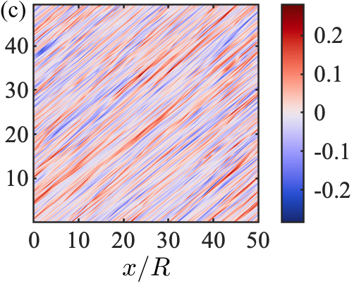
Figure 1: Space-time diagrams for $u$ (a), $v$ (b) and $w$ (c) normalised by bulk velocity $U_{b}$ at wall-normal location $y/R=0.5$.

The objective is to decompose the flow into modes which describe the complete velocity field. Therefore, the direction along which the decomposition is applied, should be chosen optimally for all velocity components. Optimality here is defined by detection of large-scale features using a minimal number of modes and is quantified by the drop of singular values along the characteristics. For each time-step the entire velocity field is stacked in one column vector which forms one of the columns of matrix $M_{(N_{ph}\times N_{t})}$ with $N_{ph}$ and $N_{t}$ corresponding to the number of spatial points in physical space and time-steps respectively. The spatio-temporal rotation is then applied to $M$ for a range of angles spaced $0.1$ radian from each other. After each rotation, a singular value decomposition is carried out and the drop of singular values are recorded as shown in figure 2a. A piecewise cubic interpolation is then used to fit a curve to all the points and to find the maximum drop which is shown with a red marker for rotation angle of $\theta_{g}=1.311$ corresponding to group velocity of $u_{g}=1.06\,U_{b}=15.5\,u_{\tau}$. This group velocity is equal to the mean radial velocity found at wall-normal location $y^{+}=1-(r/R)^{+}=44$. In figure 2b, $u_{g}$ is annotated along with the mean radial velocity profile compared with the benchmark data by El Khoury et al. (2013). By rotating the matrix $M$ by $\theta_{g}$, the data will be transformed to a moving frame of reference with the direction of characteristics serving as the new time coordinate. We search for coherent structures in planes normal to the characteristics as they travel in space and time and undergo minimal changes while maintaining their coherence.

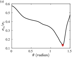
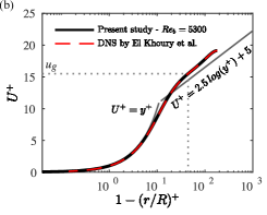
Figure 2: Drop of singular values for a range of rotation angles (a) and mean radial velocity profile compared against the benchmark data (b).

4.2 Decomposition and subspace detection

Having detected the optimal group velocity, matrix $M$ is formed using 500 timesteps with spatial resolution of $(900\times 60\times 143)$ in $(x,r,\theta)$ directions. To ensure that the dynamics of the modes are captured correctly, timestep of $dt_{\cal{C}\text{DMD}}=0.2\,t_{c}$ is chosen between the columns of $M$. Therefore, each event moving at $U_{b}$ propagates two times through the entire pipe. Transforming the data to spatio-temporal space and choosing the largest $\xi-\tau$ window in the rotated frame of reference results in the snapshots matrix in spatio-temporal space $X_{st}=\mathcal{T}(M)$, with $N_{\xi}=290$ and $N_{\tau}=843$ points along $\xi$ and $\tau$ respectively. A standard DMD is carried out to decompose $X_{st}$ into the dynamic modes $\bm{\phi}_{i}$ and their corresponding coefficients $c_{i}(\tau)$ such that $X_{st}=\varPhi C$ where $\varPhi$ and $C$ are matrices of dynamic modes and their coefficients for all timesteps. Continuous-time eigenvalues are transformed back to physical space with their real and imaginary parts representing decay rates and frequencies of the modes respectively in physical time. In figure 3, time averaged mode coefficients normalised by their $\mathcal{L}_{2}$ norm, dimensionless decay rates $\hat{d}=d/(U_{b}/R)$ and frequencies $\hat{f}=f/(U_{b}/R)$ are plotted with the modes being sorted by their decay rates. All the frequencies in spatio-temporal space are within the range of $0\leq\hat{f}_{st}<2.5$ which corresponds to $0\leq\hat{f}<10$ after transformation to physical space.

Figure 3: Dynamic mode amplitudes, decay rates and frequencies.

Next, a subset of modes is to be selected constituting a subspace (subspace I) to fulfil certain criteria which are chosen with the knowledge, that for turbulent pipe flow at this Reynolds number, there exists only one peak in the premultiplied energy spectra. The first criteria is that subspace I should accommodate energetic structures with large spatio-temporal length-scales. Therefore, it is expected to have a large contribution to the spectral peak which is known as the footprint of large-scale structures in premultiplied energy spectra. Given the nature of coherent structures, the second criteria dictates that the modes in this subspace should not possess large decay rates. This is to ensure that energetic modes with short lifetimes will not be a member of this subspace. Similarly, the candidate modes are expected to have small frequencies and not undergo strong oscillations.

We hypothesize that the modes fulfilling the mentioned criteria are expected to possess another significant property. Due to the spatio-temporal coherence of the flow captured by these modes, they are expected to have major interactions with each other, but have smaller interactions with the rest of the modes. We define this interaction in terms of the angle between the modes as well as the energy which is gained or lost by the flow as a result of presence of each two modes in a subspace. This implies that the modes in subspace I, besides being energetic, should have small angles between each other and large ones with the remaining modes.

To calculate the energy of a subspace, we first consider subspace $S$ comprised of two modes $S=\{\bm{\phi}_{1},\bm{\phi}_{2}\}$ and coefficients matrix $C_{S}$ with rows defined as $c_{1}(\tau)$ and $c_{2}(\tau)$ that can be used to obtain $X_{S}=SC_{S}$. Columns of $X_{S}$ and $C_{S}$ can be used to write for each timestep $\bm{\chi}_{S}(\tau)=S\,\bm{c}_{S}(\tau)=\bm{\phi}_{1}c_{1}(\tau)+\bm{\phi}_{2}c_{2}(\tau)$. The total energy of $S$ integrated along $\tau$ is then defined by

$$E_{S}=\sum_{\tau=1}^{N_{\tau}}\bm{c}_{S}^{*}(\tau)\,S^{*}S\,\bm{c}_{S}(\tau),$$ (2)

and energy of $S$ can be written for each time step $\tau$ as

$$\begin{split}E_{S}(\tau)&=\chi_{S}^{*}(\tau)\chi_{S}(\tau)=\bm{c}_{S}^{*}(\tau)\,S^{*}S\,\bm{c}_{S}(\tau)=\Bigl{(}c_{1}^{*}(\tau){\bm{\phi}^{*}_{1}}+c_{2}^{*}(\tau){\bm{\phi}^{*}_{2}}\Bigr{)}\Bigl{(}{\bm{\phi}_{1}}c_{1}(\tau)+{\bm{\phi}_{2}}c_{2}(\tau)\Bigr{)}\\ &=\underbrace{c_{1}^{*}(\tau){\bm{\phi}^{*}_{1}}{\bm{\phi}_{1}}c_{1}(\tau)}_{E_{1}(\tau)}+\underbrace{c_{1}^{*}(\tau)\bm{\phi}_{1}^{*}\bm{\phi}_{2}c_{2}(\tau)+c_{2}^{*}(\tau)\bm{\phi}_{2}^{*}\bm{\phi}_{1}c_{1}(\tau)}_{E_{1|2}(\tau)}+\underbrace{c_{2}^{*}(\tau)\bm{\phi}_{2}^{*}{\bm{\phi}_{2}}c_{2}(\tau)}_{E_{2}(\tau)}.\end{split}$$ (3)

The terms $E_{1}(\tau)$ and $E_{2}(\tau)$ in equation 3 correspond to the energy of modes $\bm{\phi}_{1}$ and $\bm{\phi}_{2}$ respectively at one timestep, and the term $E_{1|2}(\tau)$ represents the energy added to or taken from $X_{s}$ as a result of interaction between $\bm{\phi}_{1}$ and $\bm{\phi}_{2}$. For modes that are orthogonal to each other, the term $E_{1|2}$ vanishes and for mode pairs with small angles, $E_{1|2}$ can have large positive or negative values. Equation 3 can be generalised to the case where $\bm{\phi}_{1}$ and $\bm{\phi}_{2}$ are each separate subspaces.

To detect a subspace $\text{I}_{n}$ with $n$ most energetic modes that represents the full-field energy with fewest number of modes, and to observe how the subspace energy changes as the next energetic mode is added to it, cumulative energy is calculated for the first $n$ dominant modes, integrated along $\tau$ and normalised by the total energy as

$$\gamma_{I_{n}}=E_{I_{n}}/E_{\varPhi}.$$ (4)

and plotted in figure 4a for the first 50 modes. $E_{I_{n}}$ represents energy of subspace I possessing $n$ modes integrated over time. A fast drop is observed for the first few modes added, where two minima are observed for 4 and 6 modes resulting in subspace energy close to 1. ($\gamma_{I_{4}}=1.1$ and $\gamma_{I_{6}}=0.9$). Adding more modes increases the energy, but finally by having 11 modes, subspace energy will drop again to $\gamma_{I_{11}}=0.9$. It is clear that adding the next modes makes only minimal changes in the subspace energy.

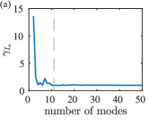
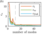
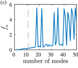
Figure 4: Cumulative energy (a), relative error (b) and frequencies (c) of the first n dominant modes.

Next, relative error is calculated for reconstruction of modes in subspace $\text{{I}}_{n}$ having $n$ modes with the corresponding coefficients matrix $C_{I_{n}}$ (equation 5). Three matrix norms have been used with $p=\{1,\infty,F\}$ for one-norm, infinity norm and frobenius norm respectively.

$$\epsilon_{n}=\|X-I_{n}C_{I_{n}}\|_{p}/\|X\|_{p}.$$ (5)

As shown in figure 4b, all relative errors reach two minima for 4 and 6 modes, increase for 7 modes, and then drop strongly for 11 modes while minimally changing beyond that point. As depicted in figure 4c, these 11 modes have very small frequencies compared to the rest of the modes.

The candidate 11 modes are highlighted in red in figure 3 with red bars. They have a small mean decay rate of $\hat{d_{I}}=0.022$ and undergo minimal oscillations with average frequency of $\hat{f_{I}}=0.086$ in the range of $0\leq\hat{f}\leq 0.2$. All the remaining modes oscillate with larger frequencies $0.22\leq\hat{f}\leq 9.86$ with the exception of mode 420 which has a large decay rate and small amplitude and therefore does not meet the criteria to be part of this subspace. 8 of the candidate modes have large amplitudes $\bar{c}/\|\bar{C}\|\,\geq 0.1$ and the rest, in spite of having smaller amplitudes $0.05\leq\bar{c}/\|\bar{C}\|\,\leq 0.07$, still possess much smaller frequencies compared to the rest of the modes. Therefore, based on the cumulative energy of subspace I, its relative error, mode amplitudes, their decay rates and frequencies, the first 11 dominant modes are chosen as members of subspace I.

Having detected a subset of energetic modes matching the mentioned criteria, we verify orthogonality of each member of this subset to modes residing inside and outside the subset. Mode-pair angles $m_{33}\angle m_{i}$ are plotted as an example in figure 5a with blue markers showing the angles that mode 33 (one of the members of subspace I) makes with all the other modes. Filled blue markers, correspond to subspace I members. It is readily seen that majority of the modes outside subspace I, are almost orthogonal to mode 33 as they accumulate close to $\alpha=90$. On the other hand, the smallest angles are made with members of subspace I ($m_{393}$ and $m_{409}$), indicating interaction between $m_{33}$ with a small decay rate, with two modes with rather larger decay rates. In figure 5b, mode pair angles $m_{237}\angle m_{i}$ and $m_{280}\angle m_{i}$ are plotted. Here it is also observed that modes outside subspace I are mostly orthogonal to $m_{237}$ and $m_{280}$. These two modes appear to make small angles with one another and rather larger angles with the rest of the modes in subspace I. A similar behaviour exists for all the modes in subspace I.

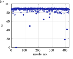
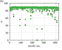
Figure 5: Angles between mode-pairs $m_{33}\angle m_{i}$ (a), $m_{237}\angle m_{i}$ and $m_{280}\angle m_{i}$ (b).

A small angle between two modes, provides the potential for a large energy interaction. But as inferred from equation 3, the term $E_{1|2}$ is dependant also on the mode coefficients besides the inner product of the two modes. Therefore in the next step, integrated energy interactions $\hat{E}_{i|k}$ are calculated between each mode ($k$) in subspace I and all the other modes ($i$) normalised by the total energy of the flow (with $\hat{.}$ denoting the normalisation). The results are plotted for $\hat{E}_{i|237}$ in figure 6a with circles and diamond markers corresponding to positive and negative values respectively. Filled markers represent modes in subspace I, which show clearly the largest interactions with $m_{237}$, some with positive and some with negative values. Apart from the contributions of the modes in subspace I (filled markers), two distinct regions also appear in this plot. A smaller number of modes can be seen at $\hat{E}_{i|237}\geq 10^{-3}$ and majority of them seem to be accumulated below this limit. This implies that there are certain modes outside subspace I, which are interacting more than the rest with $m_{237}$. These two regions appear for all the modes in subspace I indicating emergence of a second subspace, whose members are chosen based on how much energy they bring or take from the flow while interacting with subspace I. To detect the modes fitting in the new subspace, the term $\hat{E}_{i|I}$ should be calculated for all the members of subspace I as

$$\hat{E}_{i|I}=\frac{\sum\limits_{\tau=1}^{N_{\tau}}\,\sum\limits_{k=1}^{N_{I}}\Bigl{(}c^{*}_{i}(\tau)\,\bm{\phi}^{*}_{i}\bm{\phi}_{k}\,c_{k}(\tau)+c^{*}_{k}(\tau)\,\bm{\phi}^{*}_{k}\bm{\phi}_{i}\,c_{i}(\tau)\Bigr{)}}{\sum\limits_{\tau=1}^{N_{\tau}}\bm{c}^{*}(\tau)\,\varPhi^{*}\varPhi\,\bm{c}(\tau)},$$ (6)

with $N_{I}$ being the number of modes in subspace $I$, and $\tau_{i}$ and $\tau_{e}$ being the initial and last time step along $\tau$ respectively. The vector calculated using equation 6 is sorted in a descending order and modes in subspace I are excluded from the set in order to detect the largest contributions to subspace I. Cumulative energy interaction is then given for the first $p$ dominant contributions by

$$\gamma_{p,I}=\frac{\sum\limits_{j=1}^{p}\hat{E}_{j|I}}{\sum\limits_{j=1}^{N-N_{I}}\hat{E}_{j|I}},$$ (7)

with $N$ being the total number of modes, and is plotted in figure 6b. Cumulative energy contribution rises rapidly with the first 10 modes and reaches a saturation point after 60 modes, beyond which the energy does not change much by adding the remaining modes. Taking 67 modes, where a red dashed line is plotted, captures 98% of the total contribution (grey solid line).

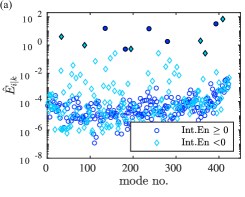
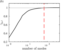
Figure 6: Normalised energy interactions between mode $m_{237}$ and all the other modes (a), and cumulative energy interaction between subspace I and the rest of the modes (b).

Having detected a second subspace, the remaining modes are grouped together to form the third subspace. Subspaces I, II and III each with 11, 67 and 346 modes amount to 3%, 15% and 82% of the total number of modes respectively. Their total kinetic energy is calculated using equation 2 being equal to $97\%$, $15\%$ and $2\%$ of the snapshots energy for the first, second and third subspaces respectively. Subspace interactions I $|$ II and II $|$ III lead to $12\%$ and $2\%$ energy loss, whereas interactions between the first and third subspaces does not cause any overall energy gain or loss.

Each subspace is then reconstructed along $\tau$. To have a visual comparison between the full-field and the subspaces, space-time diagrams are plotted for axial velocity components in figure 7 at radial location $y=0.34R$ ($y^{+}=61.5$) for one azimuthal location. Comparing the full-field with Subspace I in figures 7a and 7b, it can be seen that the large-scale flow patterns are present very well in spite of the fact that only 3% of the modes exist in this subspace. Magnitudes of negative and positive perturbations agree well with those of the full-field. Small-scale patterns are clearly missing from the reconstruction as expected. Dominant structures in this subspace appear to remain stationary along the direction of $\tau$.

Subspace II in figure 7c accommodates small-scale patterns with perturbations which are considerably less energetic than those captured in subspace I. Oblique patterns emerging show that structures here have different group velocities compared to the dominant one. Some appear to move backwards relative to the moving frame of reference indicating a slower convection velocity, whereas others move forward at higher velocity. Absence of strong vertical patterns in this figure shows that no energetic structure moving with the dominant group velocity is present in subspace II.

Subspace III with $82\%$ of the modes bears traces of some small-scale patterns similar to those in subspace II, but is mainly populated with very small-scale structures. No dominant group velocity is observable in this subspace.

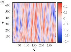
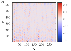
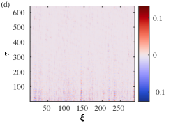
Figure 7: Space-time diagram in spatio-temporal space for the full-field (a) and subspace I (b), II (c) and III (d), at wall-normal location $y=0.34R$ and one azimuthal point

4.3 Subspaces in physical space

Each reconstructed subspace is transformed back to physical space. In figure 8, iso-surfaces of streamwise velocity component is shown for the full-field (figure 8a) and for each subspace. Similar to what was seen in the spacetime diagram, the structures in subspace I (figure 8b) appear to be similar to those in full-filed. This resemblance is observed in terms of where high and low momentum regions are located and also in terms of amplitudes of perturbations (In both subfigures iso-levels $u=\pm 0.1\,U_{b}$ are plotted). Axial length-scales in both figures perceived from the large-scale structures agree well and they will be examined in the next chapters in premultiplied spectra.

Subspace II in figure 8c on the other hand, accommodates only smaller scale structures with lower perturbation magnitudes (with iso-levels $u=\pm 0.04\,U_{b}$). The modes in this subspace were chosen based on the level of their interactions with subspace I causing large energy gains or losses. On the other hand it was shown in figure 4 that the total energy of the flow will not change drastically beyond 11 modes. This implies that although the two subspaces have large energy interactions, the overall energy of subspace I remains relatively constant. Subspace III is plotted with iso-levels $u=\pm 0.005\,U_{b}$ with two major length-scales being present in the flow, both of which are smaller than those present in the other subspaces.

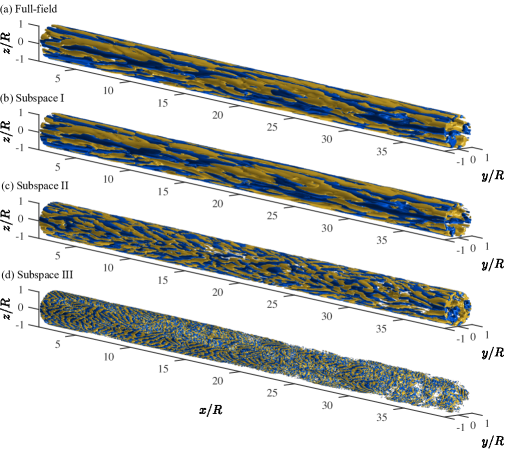
Figure 8: Iso-surfaces of axial velocity component of the full-field compared against each subspace. Iso-levels for the full-field (a) and subspace I (b) are identical with yellow and blue corresponding to $u=\pm 0.1\,U_{b}$. In subfigures (c) and (d) iso-levels of $u=\pm 0.04\,U_{b}$ and $\pm 0.005\,U_{b}$ are plotted respectively for subspaces II and III.

4.4 limitations and constraints

Due to two reasons the statistical turbulence properties of the full-field diverge from those of the snapshots matrix in physical space $X_{ph}=\mathcal{T}^{-1}(X_{st})$. The first reason is that in order for the second order statistics to converge, 4000 data realisations recorded for 400 convective timesteps have been used, whereas taking the same number of timesteps for DMD was not possible due to memory limitations. The second reason is the linear interpolation used for the spatio-temporal transformations.

The first limitation could be only partially removed using a streaming DMD (Hemati et al., 2014) and at the expense of truncating the singular values. As in this study it was intended to keep all non-zero singular values, a streaming DMD was not used. Employing higher order interpolation schemes and using larger number of timesteps, substantially increase the computation time specially at higher Reynolds numbers. It was also observed that the present setup does not bias the conclusions. Therefore, turbulence properties of the subspaces in subchapters 4.5 and 4.7 are presented using three references. The first two references are the full-field and DNS data by El Khoury et al. (2013) which are compared against each other to validate the simulation results. $X_{ph}$ serves as the third reference against which the subspaces are compared. In subchapter 4.6, the difference between the length scales in snapshots and the full-field is compensated by applying the same correction to the snapshots and all subspaces.

4.5 Contribution to Reynolds stress tensor

Contributions of each subspace to components of Reynolds stress tensor are calculated in physical space and are compared against the snapshots $X_{ph}$ which is plotted in black solid lines in figure 9. This helps to verify whether the differences between subspace statistics and the full-field, are a result of the constraints mentioned in chapter 4.4, or a property of the flow represented by the corresponding subspace. The invariants of Reynolds stress tensor are also calculated for each subspace to provide a measure of how the entire tensor compares with that of the snapshots. The first invariant being equal to the turbulent kinetic energy is already reported in the previous chapter for each subspace. The remaining two are presented in this chapter.

To ensure the accuracy and reliability of the simulated data, Reynolds stress components of the full-filed are plotted in grey solid lines and are compared against the benchmark DNS data by El Khoury et al. (2013) plotted in red dashed lines in figure 9. Stress tensor components of the full-field agree very well with those of the benchmark with the peaks being located at $y^{+}=[15,56,36,32]$ for $\langle u^{2}\rangle$, $\langle v^{2}\rangle$, $\langle w^{2}\rangle$ and $\langle uv\rangle$ respectively.

Subspace I (sI), plotted in solid blue lines, shows substantial contributions to the stress components of the snapshots with average contribution of $98\%$. The wall-normal locations of the peaks coincide with those of the snapshots at $y^{+}=[14,50,28,28]$ for $\langle u^{2}\rangle$, $\langle v^{2}\rangle$, $\langle w^{2}\rangle$ and $\langle uv\rangle$. The second and third stress tensor invariants of this subspace amount to $97\%$ and $96\%$ of those of the snapshots.

Subspace II which appears with axial length-scales smaller than sI and larger than sIII (figure 8) is plotted in green solid lines. It contributes most to the radial stress component ($22\%$) and least to the axial-radial one ($6\%$) reaching the peak values at wall-normal locations $y^{+}=28$ and $y^{+}=14$ respectively. The peaks of axial and azimuthal components occur at $y^{+}=14$ and $y^{+}=16$ with $14\%$ and $21\%$ contributions to the corresponding components of snapshots. Except for the axial component, all the peaks in this subspace have moved clearly closer to the wall compared to the snapshots. The second and third invariants of the stress tensor of this subspace are equal to $2\%$ and $0.4\%$ of those of the snapshots respectively.

Subspace III accommodating very small scale structures and represented by $82\%$ of the modes has $3.3\%$ average contribution to the diagonal Reynolds stress components and $0.1\%$ to $\langle uv\rangle$ reaching their maxima at $y^{+}=[12,92,74,31]$ respectively. This subspace contributes less than $0.02\%$ to the second and third invariants of stress tensor.

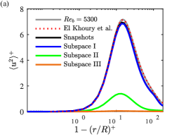
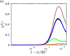
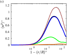
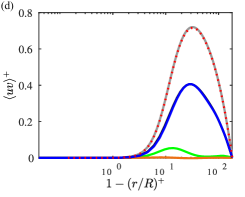
Figure 9: Reynolds stress components of the full-field compared against those of the benchmark data, each subspace and the snapshots matrix

4.6 Energy spectra

The energy content of each length-scale is analysed for each subspace using premultiplied streamwise energy spectra of velocity auto correlations ($\varphi_{uu},\varphi_{vv},\varphi_{ww}$) and cross correlation ($\varphi_{uv}$) plotted in figure 10 for the snapshots in coloured contours and black contour lines. Blue, green and orange dashed contour levels represent subspaces I, II and III respectively, each normalised by the maximum of the snapshots spectra. Blue dashed lines and black solid contour lines correspond to the same levels annotated in black. Black circle and plus markers indicate spectral peaks of the snapshots and subspace I. Coloured plus markers point to the peak locations of the corresponding subspace and coloured labels indicate the respective contour levels. The horizontal dotted and dashed lines are plotted as a reference for the commonly accepted axial length-scales of LSMs at $\lambda=2R$ and $3R$ respectively.

In the spectra of axial velocity in figure 10a, all large-scale structures are captured in subspace I and maximum energy is found for wave-length $\lambda^{+}=1006$ at $y^{+}=13.8$. Smaller structures with up to length-scale of $\lambda^{+}=300$ are also present in this subspace. Energy of wave-lengths $\lambda^{+}\leq 300$ drop compared to the snapshots at $3\leq y^{+}\leq 30$, where the solid black levels diverge from the dashed blue ones. Subspaces II and III appear with spectral peaks having smaller axial length-scales of $\lambda^{+}=304$ and $97$ at $y^{+}=11.6$ and $9.5$ with normalised peak energy of $0.37$ and $0.02$ respectively.

The radial velocity component has the shortest axial wave-length compared to the other two components as seen in figure 10b with the main peak occurring at $y^{+}=57$ for $\lambda^{+}=201$ for the snapshots and sI. The peaks of subspaces II and III emerge with smaller wave-lengths of $\lambda^{+}=134$ and $25$ at $y^{+}=24$ and $87$ with normalised peak energy of $0.3$ and $0.084$ respectively.

What can be observed in all subplots of figure 10, is that the spectral peaks found for subspace I coincide with those in the snapshots, in terms of their wall-normal locations and axial wave-lengths, with their energy content peaking on average at $99\%$ of the snapshots spectral peaks. Subspace I has captured large-scale energetic structures, and where its energy diverges from the snapshots, the next subspaces emerge with a peak. Spectral peaks in subspace II show a strong shift to the vicinity of the wall, although the shift is smaller for $k_{x}\varphi_{uu}$. Subspace III appears in all spectral maps with two low energy peaks, one below the main peak closer to the wall and one above it, with length-scales $\lambda^{+}\leq 100$. The more energetic peak belongs to the one with larger wave-length for $\varphi_{uu}$ and $\varphi_{uv}$, whereas for $\varphi_{vv}$ and $\varphi_{ww}$ it represents the smaller wave-length.

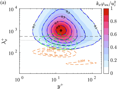
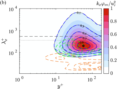
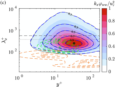
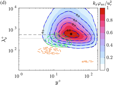
Figure 10: Premultiplied energy spectra of velocity auto correlations $\varphi_{uu}$ (a) , $\varphi_{vv}$ (b), $\varphi_{ww}$ (c) and cross correlation $\varphi_{uv}$ (d).

4.7 Anisotropy invariant map of the subspaces

We study the structure of turbulent flow in each subspace by investigating the invariants of anisotropic Reynolds stress tensor

$$a_{ij}=\frac{\tau_{ij}}{\tau_{kk}}-\frac{\delta_{ij}}{3}.$$ (8)

A triangular domain is introduced by Banerjee et al. (2007) as a barycentric anisotropy map inside which all realisable Reynolds stress invariants are located. The vertices of the triangle represent three limiting states of one-component (1c), two-component (2c) and three-component isotropic turbulence, located respectively at $\textsc{x}_{1c}=(1,0)$, $\textsc{x}_{2c}=(0,0)$ and $\textsc{x}_{3c}=(1/2,\sqrt{3}/2)$ as shown in figure 11. Moving away from the isotropic vertex on the blue edge corresponds to axi-symmetric contraction which ends up at the disc-like anisotropy at $2c$ vertex. Alternatively, moving on the black edge towards the $1c$ vertex corresponds to axi-symmetric expansion leading to needle-like anisotropy. The red edge connecting $1c$ and $2c$ vertices depicts the two-component limit. This map is defined using a linear combination of positive scalar metrics. These metrics are functions of eigen values of $a_{ij}$ being sorted as $\lambda_{1}\geq\lambda_{2}\geq\lambda_{3}$ and are used to defined the coordinate system ($x_{B},y_{B}$) given by

x_B & = C_1c x_1c + C_2c x_2c + C_3c x_3c = C_1c + C_3c 12   ,
y_B = C_1c y_1c + C_2c y_2c + C_3c y_3c = C_3c 32   ,

where

$$C_{1c}=\lambda_{1}-\lambda_{2}\,,\,\,\,C_{2c}=2(\lambda_{2}-\lambda_{3})\,,\,\,\,C_{3c}=3\lambda_{3}+1\,.$$ (9)

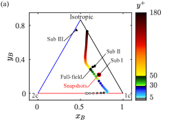
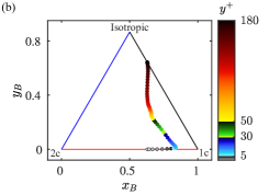
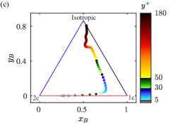
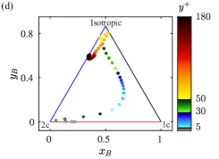
Figure 11: Isotropy invariant map of the full-field (a) subspace I (b), subspace II (c) and subspace III (d).

To have a measure of the total anisotropy, $a_{ij}$ is calculated using temporal averaging and weighted spatial averaging over all radial points and the results are plotted in annotated black markers in figure 11a. Subspaces I, II and III (shown with rectangle, diamond and triangle markers respectively) appear to be aligned on a line moving towards the isotropic state, with subspace III clearly being the most isotropic one. Snapshots averaged isotropy is plotted with a red circular marker being away from the full-field due to the fewer number of timesteps available in the snapshots. Subspace I is almost exactly on top of the red marker showing a similar anisotropy to the snapshots.

The invariant map is plotted for the full-field and for each wall-normal location in figure 11. To clearly inspect the isotropy state at each wall layer, a different colourmap has been chosen to distinguish four wall layers. Grey colourmap is set for the viscous sublayer, blue for the buffer layer between the viscous and logarithmic layer ($5\leq y^{+}\leq 30$), green for the logarithmic layer and a heat colourmap is chosen for the overlap and outer layer ($50\leq y^{+}\leq 181$). The map starts for the full-field at the wall at the two-component limit in figure 11a and moves towards the one-component vertex. At $y^{+}=10$ in the buffer layer a sharp bend is observed after which the trajectory moves towards the centre of the map where a second bend is reached at $y^{+}\approx 83$ followed by a straight path towards the isotropic vertex at the centre of the pipe.

The map for subspace I is plotted in figure 11b for each wall-normal location. The first bend takes place at the same location as the full-field whereas the second bend appears earlier at $y^{+}=65$ followed by an S shaped movement towards the isotropic state. Similarly, subspace II starts on the wall on the two-component limit but closer to disc-like isotropy moving more rapidly towards the $1c$ vertex, reaching a softer bend at $y^{+}=10$. After that, the trajectory follows a straight line approaching the axi-symmetric expansion limit where the second bend takes place moving away from the black edge at $y^{+}\approx 83$. A third bend is reached at $y^{+}\approx 120$ after which the flow approaches the isotropic state close to the pipe axis.

Subspace III shows a very different behaviour starting on the two-component limit and moving towards the disc-like anisotropy where it almost reaches the $2c$ vertex in the viscous sublayer at $y^{+}=1.3$. A very soft bend takes place at $7.5\leq y^{+}\leq 14$ followed by a path towards the isotropic state. In the overlap layer at $57\leq y^{+}\leq 65$ the trajectory gets closest to the isotropic state after which it departs towards the axi-symmetric contraction limit at the pipe axis.

5 Summary and conclusions

5.1 Summary

A characteristic DMD is carried out on DNS data of turbulent pipe flow at $\Rey_{b}=5300$ decomposing three velocity components along the characteristics of the flow corresponding to the group velocity of $u_{g}=1.1\,U_{b}$. Three subspaces are extracted and their contributions to stream wise energy spectra and components of Reynolds stress tensor are investigated along with the anisotropy invariant maps to compare the structure of turbulence in each subspace.

Subspace I being the most energetic one is comprised of 11 modes ($3\%$ of the total modes) and is detected based on three main criteria: the mode amplitudes, cumulative energy of the constituent modes and the relative error with respect to the snapshots matrix. This subspace undergoes minimal oscillations in space and time having a very small average frequency of $\hat{f_{I}}=0.086$ and it decays slowly with the mean decay rate of $\hat{d_{I}}=0.022$. The modes in this subspace form small angles with one another and larger ones with the rest of the modes, indicating large energy interactions inside the subspace and small interactions with the rest of the modes while maintaining the total kinetic energy of the subspace. The axial wave lengths and wall normal locations of the spectral peaks in this subspace coincide accurately with those of the snapshots. Subspace I contributes $97\%$ to the turbulent kinetic energy and $99\%$ to the $\langle uv\rangle$ component of Reynolds stress tensor.

Subspace II is detected with 67 modes ($15\%$ of the total modes) based on cumulative energy interactions of its members to subspace I. This subspace oscillates almost 25 times faster than subspace I with average frequency of $\hat{f}_{II}=2.1$ and decays almost twice faster with average decay rate of $\hat{d}_{II}=0.043$. The spectral peaks of sII in all axial energy spectra appear closer to the wall in the buffer layer with the peak value amounting to $30\%-40\%$ of the snapshots peak. Only small scale flow features are present in this subspace with spectral peaks corresponding to maximum wave length of $\lambda^{+}=304$ for the stream wise component and minimum of $\lambda^{+}=134$ for the radial one. The peaks of Reynolds stress profiles emerge closer to the wall for all the components having total contribution of $6\%$ to $\langle uv\rangle$ component of Reynolds stress tensor. This subspace contributes $15\%$ to kinetic energy while its interactions with subspaces I and III causes $12\%$ and $2\%$ of energy loss respectively. There are length scales which are present in sI and sII implying that all structures with the same length scales do not necessarily have the same contributions to Reynolds stress tensor or kinetic energy.

The remaining 346 modes ($82\%$) constitute subspace III having only minimal energy contributions to the first two subspaces. It oscillates on average more than two times faster than subspace II with frequency of $\hat{f}_{III}=5.61$ and decays with average decay rate of $\hat{d}_{III}=0.016$. Only very small scale flow features with low energy levels are observed here which are oscillating fast but they are persistent in space and time. This subspace has $2\%$ contribution to the kinetic energy and close to no overall interaction with subspace I. It contributes to $0.1\%$ of $\langle uv\rangle$ and shows the most isotropic behaviour among all the subspaces specially in the overlap layer and a distinct disc-like anisotropy in the viscous sublayer.

5.2 Conclusions

The wave-like definition of coherent structures in a characteristic frame of reference in transport-dominated turbulent flows proves to be very efficient for the two following reasons: The main features of pipe flow at $Re_{b}=5300$ is captured accurately with only $3\%$ of the modes which form an almost orthogonal subspace to the rest of the modes. This subspace reproduces $97\%$ of the turbulent kinetic energy of the full flow, and more than $96\%$ of the invariants of the Reynolds stress tensor. Its spectral signature matches the snapshots in terms of wall-normal locations and wavelengths of the premultiplied energy spectra.

The second reason is that the remaining modes can be further divided into two subspaces based on their cumulative energy contributions to subspace I. The Third subspace accommodates very small scales with short turn-over times and persists as a turbulent background motion. The second subspace lives in between the mentioned subspaces I and III having faster decay rates than the other two subspaces with their spectral peak length scales being substantially smaller than the first and substantially larger than the third subspace.

We speculate that at higher Reynolds numbers more modes would be needed to build subspace I and the scale separation between the subspaces would increase. We base our speculation on the fact that the flow becomes more complex and wider range of group velocities would be present in the flow.

[Funding]This joint study was part of the Priority Programme SPP 1881 Turbulent Superstructures of the Deutsche Forschungsgemeinschaft and funded by grant no. SE 824/33-1 (J.S and A.Sh) and grant no. EG100/24-2 (Ch. E.)

[Acknowledgements]All simulations in this study have been carried out on Norddeutscher Verbund für Hoch- und Höchstleistungsrechnen (HLRN) with project id: bbi00011, using the code of our project partners within the SPP 1881 (grant no. AV120/3-2).

[Declaration of interests] The authors report no conflict of interest.

References

- Bailey & Smits (2010) Bailey, S. C. C. & Smits, A. J. 2010 Experimental investigation of the structure of large- and very-large-scale motions in turbulent pipe flow. Journal of Fluid Mechanics 651, 339–356.
- Banerjee et al. (2007) Banerjee, S., Krahl, R., Durst, F. & Zenger, Ch. 2007 Presentation of anisotropy properties of turbulence, invariants versus eigenvalue approaches. Journal of Turbulence 8, N32.
- Bauer et al. (2019) Bauer, C., von Kameke, A. & Wagner, C. 2019 Kinetic energy budget of the largest scales in turbulent pipe flow. Phys. Rev. Fluids 4, 064607.
- Del Álamo & Jiménez (2006) Del Álamo, J. C. & Jiménez, J. 2006 Linear energy amplification in turbulent channels. Journal of Fluid Mechanics 559, 205–213.
- El Khoury et al. (2013) El Khoury, G. K., Schlatter, P., Noorani, A., Fischer, P., Brethouwer, G. & Johansson, A. 2013 Direct numerical simulation of turbulent pipe flow at moderately high reynolds numbers. Flow, Turbulence and Combustion 91, 475–495.
- Guala et al. (2006) Guala, M., Hommema, S. E. & Adrian, R. J. 2006 Large-scale and very-large-scale motions in turbulent pipe flow. Journal of Fluid Mechanics 554, 521–542.
- Hellström & Smits (2014) Hellström, Leo H. O. & Smits, Alexander J. 2014 The energetic motions in turbulent pipe flow. Physics of Fluids 26 (12).
- Hemati et al. (2014) Hemati, M., Williams, M. & Rowley, C. 2014 Dynamic mode decomposition for large and streaming datasets. Physics of Fluids 26.
- Hugues & Randriamampianina (1998) Hugues, Sandrine & Randriamampianina, Anthony 1998 An improved projection scheme applied to pseudospectral methods for the incompressible navier-stokes equations. International Journal for Numerical Methods in Fluids 28, 501–521.
- Jiménez & Moin (1991) Jiménez, J. & Moin, P. 1991 The minimal flow unit in near-wall turbulence. Journal of Fluid Mechanics 225, 213–240.
- Kim & Adrian (1999) Kim, K. C. & Adrian, R. J. 1999 Very large-scale motion in the outer layer. Physics of Fluids 11.
- Kline et al. (1967) Kline, S. J., Reynolds, W. C., Schraub, F. A. & Runstadler, P. W. 1967 The structure of turbulent boundary layers. Journal of Fluid Mechanics 30 (4), 741–773.
- Lumley (1967) Lumley, J. L. 1967 The structure of inhomogeneous turbulent flows. Atmospheric turbulence and radio wave propagation pp. 166–178.
- López et al. (2020) López, Jose Manuel, Feldmann, Daniel, Rampp, Markus, Vela-Martín, Alberto, Shi, Liang & Avila, Marc 2020 nscouette – a high-performance code for direct numerical simulations of turbulent taylor–couette flow. SoftwareX 11, 100395.
- Marusic et al. (2010) Marusic, I., McKeon, B., Monkewitz, Peter, Nagib, Hassan, Smits, Alexander & Sreenivasan, K. 2010 Wall-bounded turbulent flows at high reynolds numbers: Recent advances and key issues. Physics of Fluids 22.
- Monty et al. (2009) Monty, J. P., Hutchins, N., NG, H. C. H., Marusic, I. & Cchon, M. S. 2009 A comparison of turbulent pipe, channel and boundary layer flows. Journal of Fluid Mechanics 632, 431–442.
- Reiss et al. (2018) Reiss, J., Schulze, P., Sesterhenn, J. & Mehrmann, V. 2018 The shifted proper orthogonal decomposition: A mode decomposition for multiple transport phenomena. SIAM Journal on Scientific Computing 40 (3), A1322–A1344.
- Rosenberg et al. (2013) Rosenberg, B. J., Hultmark, M., M. Vallikivi, S. C. C. Bailey & Smits, A. J. 2013 Turbulence spectra in smooth- and rough-wall pipe flow at extreme reynolds numbers. J. Fluid Mech. 731, 46–63.
- Rowley & Marsden (2000) Rowley, C. W. & Marsden, J. E. 2000 Reconstruction equations and the karhunen–loève expansion for systems with symmetry. Physica D: Nonlinear Phenomena 142 (1–2), 1 – 19.
- Schmid (2010) Schmid, P. J. 2010 Dynamic mode decomposition of numerical and experimental data. J. Fluid Mech. 656, 5–28.
- Schmid & Sesterhenn (2008) Schmid, P. J. & Sesterhenn, J. 2008 Dynamic mode decomposition of numerical and experimental data. Amer. Phys. Soc.,61st APS meeting p. 208.
- Sesterhenn & Shahirpour (2019) Sesterhenn, J. & Shahirpour, A. 2019 A characteristic dynamic mode decomposition. Theoretical and Computational Fluid Dynamics 33.
- Shi et al. (2015) Shi, Liang, Rampp, Markus, Hof, Björn & Avila, Marc 2015 A hybrid mpi-openmp parallel implementation for pseudospectral simulations with application to taylor–couette flow. Computers & Fluids 106, 1–11.
- Sirovich (1987) Sirovich, L. 1987 Turbulence and the dynamics of coherent structures. i - coherent structures. ii - symmetries and transformations. iii - dynamics and scaling. Quarterly of Applied Mathematics 45, 561–571.
- Toh & Itano (2005) Toh, S. & Itano, T. 2005 Interaction between a large-scale structure and near-wall structures in channel flow. Journal of Fluid Mechanics 524, 249–262.
- Vallikivi et al. (2015) Vallikivi, M., Ganapathisubramani, B. & Smits, A. J. 2015 Spectral scaling in boundary layers and pipes at very high reynolds numbers. J. Fluid Mech. 771, 303–326.
- del Álamo & Jiménez (2006) del Álamo, J. C. & Jiménez, J. 2006 Linear energy amplification in turbulent channels. Journal of Fluid Mechanics 559, 205–213.