3D Reconstruction with Generalizable Neural Fields using Scene Priors

Abstract

High-fidelity 3D scene reconstruction has been substantially advanced by recent progress in neural fields. However, most existing methods train a separate network from scratch for each individual scene. This is not scalable, inefficient, and unable to yield good results given limited views. While learning-based multi-view stereo methods alleviate this issue to some extent, their multi-view setting makes it less flexible to scale up and to broad applications. Instead, we introduce training generalizable Neural Fields incorporating scene Priors (NFPs). The NFP network maps any single-view RGB-D image into signed distance and radiance values. A complete scene can be reconstructed by merging individual frames in the volumetric space WITHOUT a fusion module, which provides better flexibility. The scene priors can be trained on large-scale datasets, allowing for fast adaptation to the reconstruction of a new scene with fewer views. NFP not only demonstrates SOTA scene reconstruction performance and efficiency, but it also supports single-image novel-view synthesis, which is underexplored in neural fields. More qualitative results are available at: https://oasisyang.github.io/neural-prior.

1 Introduction

Reconstructing a large indoor scene has been a long-standing problem in computer vision. A common approach is to use the Truncated Signed Distance Function (TSDF) (Zhou et al., 2018; Dai et al., 2017b) with a depth sensor on personal devices. However, the discretized representation with TSDF limits its ability to model fine-grained details, e.g., thin surfaces in the scene. Recently, a continuous representation using neural fields and differentiable volume rendering (Guo et al., 2022; Yu et al., 2022; Azinović et al., 2022; Wang et al., 2022b; Li et al., 2022) has achieved impressive and detailed 3D scene reconstruction. Although these results are encouraging, Although these results are encouraging, all of them require training a distinct network for every scene, leading to extended training durations with the demand of a substantial number of input views.

To tackle these limitations, several works learn a generalizable neural network so that the representation can be shared among difference scenes (Wang et al., 2021b; Zhang et al., 2022; Chen et al., 2021; Long et al., 2022; Xu et al., 2022). While these efforts scale up training on large-scale scene datasets, introduce generalizable intermediate scene representation, and significantly cut down inference time, they all rely on intricate fusion networks to handle multi-view input images at each iteration. This adds complexity to the training process and limits flexibility in data preprocessing.

In this paper, we propose to perform 3D reconstruction by learning generalizable Neural Fields using scene Priors (NFPs). Such priors are largely built upon depth-map inputs (given posed RGB-D images). By leveraging the priors, our NFPs network allows for a simple and flexible design with single-view inputs during training, and it can efficiently adapt to each novel scene using fewer input views. Specifically, full scene reconstruction is achieved by directly merging the posed multi-view frames and their corresponding fields from NFPs, without the need for learnable fusion blocks.

A direct way to generalize per-scene Nerf optimization is to encode each single-view input image into an intermediate representation in the volumetric space. Yet, co-learning the encoder and the NeRF presents significant challenges. Given that a single-view image captures only a thin segment of a surface, it becomes considerably harder to discern the geometry compared to understanding the texture. Thus, to train NFPs, we introduce a two-stage paradigm: (i) We train a geometric reconstruction network to map depth images to local SDFs; (ii) We adopt this pre-trained network as a geometric prior to support the training of a separate color reconstruction network, as a texture prior, in which the radiance function can be easily learned with volumetric rendering (Wang et al., 2021a; Yariv et al., 2021), given the SDF prediction.

Dense voxel grids are a popular choice in many NeRF-based rendering techniques (Yen-Chen et al., 2020; Chen et al., 2021; Liu et al., 2020; Huang et al., 2021; Takikawa et al., 2021; Sun et al., 2022b; Wang et al., 2022b). However, for the single-view input context, they fall short for two main reasons. First, the single-view image inherently captures just a thin and confined segment of surfaces, filling only a minuscule fraction of the entire voxel space. Second, dense voxel grids employ uniform sampling, neglecting surface priors like available depth information. Instead, we resort to a surface representation: we build a set of projected points in the 3D space as keypoint, from where a continuous surface can be decoded. The keypoint representation spans a compact 2D surface representation, allowing dense sampling close to the surface, which significantly enhances scalability.

NFPs can easily facilitate further fine-tuning on large-scale indoor scenes. Given the pretrained geometry and texture network as the scene prior, the single-scene reconstruction can be performed by optimizing the aggregated surface representation and the decoders. With coarse reconstruction from the generalized network and highly compact surface representation, our approach achieves competitive scene reconstruction and novel view synthesis performance with substantially fewer views and faster convergence speed. In summary, our contributions include:

• We propose NFPs, a generalizable scene prior that enables fast, large-scale scene reconstruction.

• NFPs facilitate (a) single-view, across-scene input, (b) direct fusion of local frames, and (c) efficient per-scene fine-tuning.

• We introduce a continuous surface representation, taking advantage of the depth input and avoiding redundancy in the uniform sampling of a volume.

• With the limited number of views, we demonstrate competitive performance on both the scene reconstruction and novel view synthesis tasks, with substantially superior efficiency than existing approaches.

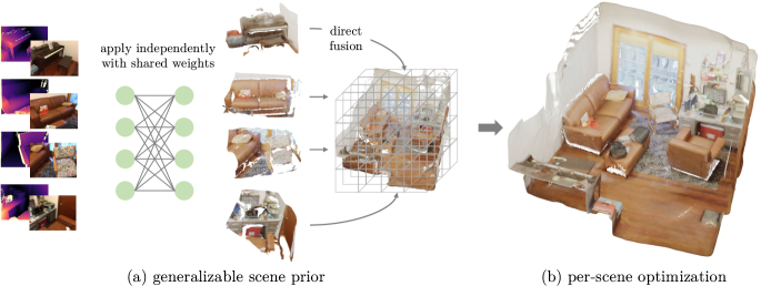
Figure 1: We propose Neural Fields scene Prior (NFP) to enable fast reconstruction of geometry and texture of indoor scenes. Our method first (a) learns a generalizable network as a scene prior that obtains a coarse scene reconstruction in a feed-forward manner. Next, we directly fuse the per-view results and (b) perform per-scene optimization in a more accurate and efficient way leading to high-quality surface reconstruction and realistic texture reconstruction.

2 Related Work

Reconstructing and rendering large-scale indoor scenes is crucial for various applications. Depth sensors, on the other hand, are becoming increasingly common in commercial devices, such as Kinect (Zhang, 2012; Smisek et al., 2013), iPhone LiDAR (Nowacki & Woda, 2019), etc. Leveraging depth information in implicit neural representations is trending. We discuss both these topics in detail, in the following.

Multi-view scene reconstruction. Reconstructing 3D scenes from images was dominated by multi-view stereo (MVS) (Schönberger et al., 2016; Schonberger & Frahm, 2016), which often follows the single-view depth estimation (e.g., via feature matching) and depth fusion process (Newcombe et al., 2011; Dai et al., 2017b; Merrell et al., 2007). Recent learning-based MVS methods (Cheng et al., 2020; Düzçeker et al., 2020; Huang et al., 2018; Luo et al., 2019) substantially outperform the conventional pipelines. For instance, Yao et al. (2018); Luo et al. (2019) build the cost-volume based on 2D image features and use 3D CNNs for better depth estimation. Another line of works (Sun et al., 2021; Bi et al., 2017) fuse multi-view depth and reconstruct surface meshes using techniques such as TSDF fusion. Instead of fusing the depth, Wei et al. (2021), Wang et al. (2021b), Zhang et al. (2022), and Xu et al. (2022) directly aggregate multi-view inputs into a radiance field for coherent reconstruction. The multi-view setting enables learning generalizable implicit representation, however, their scalability is constrained as they always require multi-view RGB/RGB-D data during training. Our approach, for the first time, learns generalizable scene priors from single-view images with substantially improved scalability.

Neural Implicit Scene Representation. A growing number of approaches (Yariv et al., 2020; Wang et al., 2021a; Yariv et al., 2021; Oechsle et al., 2021; Niemeyer et al., 2020; Sun et al., 2022a) represent a scene by implicit neural representations. Although these methods achieve impressive reconstruction of objects and scenes with small-scale and rich textures, they hardly faithfully reconstruct large-scale scenes due to the shape-radiance ambiguity suggested in (Zhang et al., 2020; Wei et al., 2021). To address this issue,  Guo et al. (2022) and  Yu et al. (2022) attempt to build the NeRF upon a given geometric prior, i.e., sparse depth maps and pretrained depth estimation networks. However, these methods take a long time to optimize on an individual scene. As mentioned previously, generalizable NeRF representations with mutli-view feature aggregation are studied (Chen et al., 2021; Wang et al., 2021b; Zhang et al., 2022; Johari et al., 2022; Xu et al., 2022). However, they still focus on reconstructing the scene’s appearance, e.g., for novel view synthesis, but cannot guarantee high-quality surface reconstruction.

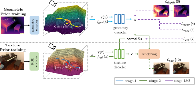
Figure 2: Overview of NFP. Given the RGBD input, we first extract the geometric and texture pixel feature using two encoders (Sec. 3.1). Then, we construct the continuous surface representation upon the discrete surface feature (Sec. 3.2). Next, we introduce a two-stage paradigm to learn the generalizable geometric and texture prior, optimized via multiple objectives (Sec. 3.3).

Depth-supervised reconstruction and rendering. With the availability of advanced depth sensors, many approaches seek depth-enhanced supervision of NeRF (Azinović et al., 2022; Li et al., 2022; Zhu et al., 2022; Sucar et al., 2021; Yu et al., 2022; Williams et al., 2022; Xu et al., 2022; Deng et al., 2022) since depth information is more accessible. For instance,  Azinović et al. (2022) enables detailed reconstruction of large indoor scenes by comparing the rendered and input RGB-D images. Unlike most methods that use depth as supervision,  Xu et al. (2022) and  Williams et al. (2022) build the neural field conditioned on the geometric prior. For example, Point-NeRF pretrains a monocular depth estimation network and generates a point cloud by lifting the depth prediction. Compared to ours, their geometric prior is less integrated into the main reconstruction stream since it is separately learned and detached. Furthermore, these methods only consider performing novel view synthesis (Xu et al., 2022; Deng et al., 2022), where the geometry is not optimized, or perform pure geometric (Yu et al., 2022; Li et al., 2022; Williams et al., 2022; Azinović et al., 2022) reconstruction. In contrast, our approach makes the scene prior and the per-scene optimization a unified model that enables more faithful and effficient reconstruction for both color and geometry.

3 Method

Given a sequence of RGB-D images and their corresponding camera poses, our goal is to perform fast and high-quality scene reconstruction. To this end, we learn a generalizable neural scene prior, which encodes an RGB image and its depth map as continuous neural fields in 3D space, and decodes them into signed distance and radiance values. As illustrated in Fig. 2, we first extract generalizable surface features from geometry and texture encoders (Sec. 3.1). Then, pixels with depth values are back-projected to the 3D space as keypoints, from which continuous fields can be built with the proposed surface representation (Sec. 3.2). Motivated by previous works (Wang et al., 2021a; Yariv et al., 2021), we utilize two separate MLPs to decode the geometry and texture representations, which are further rendered into RGB and depth values (Sec. 3.3). To obtain high-quality surface reconstruction, we further propose to optimize the neural representation on top of the learned geometric and texture prior for a specific scene (Sec. 3.4).

3.1 Constructing surface feature

Given an RGB-D image $\{\mathrm{I},\mathrm{D}\}$, we first project the depth map into 3D point clouds in the world coordinate system using its camera pose $\{\mathrm{R,t}\}$ and intrinsic matrix $\mathrm{K}$. We sub-sample $M$ points via Farthest Point Sampling (FPS), denoted as $\{p_{m}\},m\in[0,M-1]$, which are used as keypoints representing the discrete form of surfaces. We extract generalizable point-wise geometry and texture features, as described below, which are further splatted onto these keypoints. Both encoders are updated when training the NFP.

Geometry encoder. For each surface point, we apply the K-nearest neighbor (KNN) algorithm to find $K-1$ points and construct a local region with $K$ points. Thus, we obtain a collection of $M$ local regions, $\{p_{m},\{p_{k}\}_{k\in\Psi_{m}}\},\forall m\in[0,M-1]$, where $\Psi_{m}$ is the neighbor index set of point $p_{m}$ and $|\Psi_{m}|=K-1$. Then, we utilize a stack of PointConv (Wu et al., 2019) layers to extract the geometry feature from each local region $f_{\mathrm{m}}^{\mathrm{geo}}=\mathrm{PointConv}(\{p_{m},\{p_{k}\}_{k\in N_{m}}\})$.

Texture encoder. In addition, we extract RGB features for the keypoints via a 2D convolutional neural network. In particular, we feed an RGB image $I$ into an UNet (Ronneberger et al., 2015) with ResNet34 (He et al., 2016) as the backbone, which outputs a dense feature map. Then, we splat the pixel-wise features $f_{\mathrm{m}}^{\mathrm{tex}}$ onto the keypoints, according to the projection location of the surface point $p_{m}$ from the image plane. Thus, each surface point is represented by both a geometry feature and a texture feature, denoted by $f(\mathrm{p}_{\mathrm{m}})=[f_{\mathrm{geo}}(\mathrm{p}_{\mathrm{m}}),f_{\mathrm{tex}}(\mathrm{p}_{\mathrm{m}})]$.

3.2 Continuous Surface Implicit Representation

Given the lifted keypoints and their projected geometry and texture features, in this section, we introduce how to construct continuous implicit fields conditioned on such discrete representations. We follow a spatial interpolation strategy: for any query point $\mathrm{x}$ (e.g., in a typical volume rendering process, it can be a sampled point along any ray), we first find the $K$ nearest surface points $\{p_{v}\}_{v\in V}$, where $V$ is a set of indices of the neighboring surface points. Then, the query point’s feature can be obtained via aggregation of its neighboring surface points. In particular, we apply distance-based spatial interpolation as

$$f(\mathrm{x})=\frac{\sum_{v\in V}\omega_{v}f(\mathrm{p}_{v})}{\sum_{v\in V}\omega_{v}};\quad\omega_{v}=\exp{(-||\mathrm{x}-\mathrm{p}_{v}||)},$$ (1)

where $f(\mathrm{x})$ represents either the geometry $f_{\mathrm{geo}}(\mathrm{x})$ or the texture $f_{\mathrm{tex}}(\mathrm{x})$ feature, and $p_{v}$ is the position of the $v$-th neighbouring keypoint. With distance-based spatial interpolation, we establish continuous implicit fields for any point from the discrete keypoints.

The continuous representation suffers from two drawbacks: First, when a point is far away from the surface, $f(\mathrm{x})$ is no longer a valid representation, but will still contribute to decoding and rendering. Second, the distance $\omega_{v}$ is agnostic to the tangent direction and hence is likely to blur the boundaries. To mitigate the first problem, we incorporate an additional MLP layer that takes into account both the original surface feature $f(\mathrm{p}_{v})$ and its relative distance to the query point $\mathrm{x}-\mathrm{p}_{v}$, and outputs a distance-aware surface feature $f(\mathrm{p}_{v}^{x})=\mathbf{MLP}(f(\mathrm{p}_{v}),\mathrm{x}-\mathrm{p}_{v})$. Subsequently, this refined surface feature $f(\mathrm{p}_{v}^{x})$ replaces the original surface feature in Eq. 1 to obtain the feature of query point $\mathrm{x}$. In addition, we ensure that the sampled points lie near the surface via importance sampling. We resolve the second issue via providing the predicted normal to the decoders as an input. We refer to Sec. 3.3 and 3.4 for details.

3.3 Generalizable Neural Scene Prior

To reconstruct both geometry and texture, i.e., a textured mesh, a direct way is to decode the geometry and texture surface representation (Sec. 3.2) into signed distance and radiance values, render them into RGB and depth pixels (Guo et al., 2022; Yu et al., 2022), and then supervise them by the ground-truth RGB-D images. Unlike the multi-view setting that covers a significant portion of the volumetric space, the single-view input only encompasses a small fraction of it. From our experiments, we found that the joint training approach struggles to generate accurate geometry.

Hence, we first learn a geometric network that maps any depth input to its corresponding SDF (Sec. 3.3.1). Once a coarse surface is established, learning the radiance function initialized by it becomes much easier – we pose it in the second stage where a generalizable texture network is introduced similarly (Sec. 3.3.2).

3.3.1 Generalizable Geometric Prior

We represent scene geometry as a signed distance function, where in our case, it is conditioned on the geometric surface representation $f_{\mathrm{geo}}(x)$ to allow for generalization ability across different scenes. Specifically, along each back-projected ray with camera center $\mathbf{o}$ and ray direction $\mathbf{r}$, we sample $N$ points as $\mathrm{x}_{i}=\mathbf{o}+d_{i}\mathbf{r},\ \forall i\in[0,N-1]$. For each sampled points $\mathrm{x}_{i}$, its geometry feature $f_{\mathrm{geo}}(\mathrm{x}_{i})$ can be computed by equation 1. Then, the geometry decoder $\phi_{\mathrm{G}}$, taking the point position and its geometry feature as inputs, maps each sampled point to a signed distance, which is defined as $\mathbf{s}(\mathrm{x}_{i})=\phi_{\mathrm{G}}(f_{\mathrm{geo}}(\mathrm{x}_{i}),\mathrm{x}_{i})$. Note that we also apply positional encoding $\gamma(\cdot)$ to the point position as suggested in Mildenhall et al. (2020). We omit it for brevity.

Following the formulation of NeuS (Wang et al., 2021a), the estimated depth value $\hat{d}$ is the expected values of sampled depth $d_{i}$ along the ray:

$$\hat{d}=\sum_{i}^{N}{T_{i}\alpha_{i}d_{i}};\quad T_{i}=\prod_{j=1}^{i-1}(1-\alpha_{j})$$ (2)

$$\alpha_{i}=\max\left(\frac{\sigma_{s}(\mathbf{s}(\mathrm{x}_{i}))-\sigma_{s}(\mathbf{s}(\mathrm{x}_{i+1}))}{\sigma_{s}(\mathbf{s}(\mathrm{x}_{i}))},0\right),$$

where $T_{i}$ represents the accumulated transmittance at point $\mathrm{x}_{i}$, $\alpha_{i}$ is the opacity value and $\sigma_{s}$ is a Sigmoid function modulated by a learnable parameter $s$.

Geometry objectives. To optimize the generalizable geometric representation, we apply a pixel-wise rendering loss on the depth map,

$$\mathcal{L}_{\mathrm{depth}}=|\hat{d}-\mathrm{D}(x,y)|.$$ (3)

Inspired by (Azinović et al., 2022; Li et al., 2022), we approximate ground-truth SDF based on the distance to observed depth values along the ray direction, $b(\mathrm{x}_{i})=\mathrm{D}(x,y)-d_{i}$. Thus, for points that fall in the near-surface region ($|b(\mathrm{x}_{i})|\leq\tau$, $\tau$ is a truncation threshold), we apply the following approximated SDF loss

$$\mathcal{L}_{\mathrm{near}}=|\mathbf{s}(\mathrm{x}_{i})-b(\mathrm{x}_{i})|$$ (4)

We also adopt a free-space loss (Ortiz et al., 2022) to penalize the negative and large positive predictions.

$$\vspace{-1mm}\mathcal{L}_{\mathrm{free}}=\begin{aligned} &\max\left(0,e^{-\epsilon\mathbf{s}(\mathrm{x}_{i})}-1,\mathbf{s}(\mathrm{x}_{i})-b(\mathrm{x}_{i})\right),\end{aligned}$$ (5)

where $\epsilon$ is the penalty factor. Then, our approximated SDF loss is

$$\mathcal{L}_{\mathrm{sdf}}=\left\{\begin{aligned} \mathcal{L}_{\mathrm{near}}\quad&\mathrm{if}\ b(\mathrm{x}_{i})\leq|\tau|\\ \mathcal{L}_{\mathrm{free}}\quad&\mathrm{otherwise}\end{aligned}\right.$$ (6)

The approximated SDF values provide us with more explicit and direct supervision than the rendering depth loss (Eq. equation 3).

Surface regularization. To avoid artifacts and invalid predictions, we further use the Eikonal regularization term (Yariv et al., 2021; Ortiz et al., 2022; Wang et al., 2021a), which aims to encourage valid SDF values via the following,

$$\mathcal{L}_{\mathrm{eik}}=||\nabla_{\mathrm{x}_{i}}\mathbf{s}(\mathrm{x}_{i})-1||_{2}^{2},$$ (7)

where $\nabla_{\mathrm{x}_{i}}\mathbf{s}(\mathrm{x}_{i})$ is the gradient of predicted SDF w.r.t. the sampled point $\mathrm{x}_{i}$.

Therefore, we update the geometry encoder and decoder with the generalizable geometry loss as following,

$$\mathcal{L}_{\mathrm{geo}}=\lambda_{\mathrm{depth}}\mathcal{L}_{\mathrm{depth}}+\lambda_{\mathrm{sdf}}\mathcal{L}_{\mathrm{sdf}}+\lambda_{\mathrm{eik}}\mathcal{L}_{\mathrm{eik}}$$ (8)

3.3.2 Generalizable Texture Prior

We build the 2nd stage – the generalizable texture network following the pretrained geometry network, as presented in Sec. 3.3.1, which offers the SDF’s prediction as an initialization. Specifically, we learn pixel-wise RGB features, as described in Sec. 3.1, and project them onto the corresponding keypoints. Following the spatial interpolation method in Sec. 3.2, we query the texture feature of any sampled point in 3D space. As aforementioned, the spatial interpolation in Eq. equation 1 is not aware of the surface tangent directions. For instance, a point at the intersection of two perpendicular planes will be interpolated with keypoints coming from both planes. Thus, representations at the boundary regions can be blurred. To deal with it, we further concatenate the surface normal $\nabla_{\mathrm{x}_{i}}\mathbf{s}(\mathrm{x}_{i})$ predicted in the first stage with the input to compensate for the missing information.

With a separate texture decoder $\phi_{\mathrm{tex}}$, the color of point $\mathrm{x}_{i}$ is estimated, conditioned on the texture feature $f_{\mathrm{tex}}(\mathrm{x}_{i})$ and the surface normal $\nabla_{\mathrm{x}_{i}}\mathbf{s}(\mathrm{x}_{i})$ ,

$$\mathbf{c}(\mathrm{x}_{i})=\phi_{\mathrm{tex}}(f_{\mathrm{tex}}(\mathrm{x}_{i}),\mathbf{r},\nabla_{\mathrm{x}_{i}}\mathbf{s}(\mathrm{x}_{i})),$$ (9)

where $\mathbf{r}$ is the ray direction. Here we omit the positional encoding of point’s position and ray direction for conciseness. Therefore, the predicted pixel color can be expressed as $\hat{\mathbf{c}}=\sum_{i}^{N}T_{i}\alpha_{i}\mathbf{c}_{i}$, where $T_{i}$ and $\alpha_{i}$ are defined same as Eq. equation 2. We supervise the network by minimizing the $\mathrm{L}2$ loss between the rendered pixel RGB values and their ground truth values

$$\mathcal{L}_{\mathrm{rgb}}=||\hat{\mathbf{c}}-\mathrm{I}(x,y)||_{2}^{2}.$$ (10)

Meanwhile, we jointly learn the geometry network including the PointConv encoder and geometry decoder introduced in Sec. 3.2, via the same $\mathcal{L}_{\mathrm{geo}}$. Thus, the total loss function for generalizable texture representation learning is

$$\mathcal{L}_{\mathrm{tex}}=\lambda_{\mathrm{depth}}\mathcal{L}_{\mathrm{depth}}+\lambda_{\mathrm{sdf}}\mathcal{L}_{\mathrm{sdf}}+\lambda_{\mathrm{eik}}\mathcal{L}_{\mathrm{eik}}+$$ (11)

$$\lambda_{\mathrm{rgb}}\mathcal{L}_{\mathrm{rgb}}.$$

During volumetric rendering, to restrict the sampled points from being concentrated on the surface, we perform importance sampling based on: (i) the predicted surface as presented in Wang et al. (2021a), and (ii) the input depth map. More details are in the supplementary material.

3.4 Prior-guided Per-scene Optimization

To facilitate large-scale, high-quality scene reconstruction, we can further finetune the pretrained generalizable geometric and texture prior on individual scenes, with multi-view frames. Specifically, we first directly fuse the geometry and texture feature of multi-view frames via the scene prior networks. No further learnable modules are required, in contrast, to (Chen et al., 2021; Zhang et al., 2022; Li et al., 2022). Then, we design a prior-guided pruning and sampling module, which lets optimization happens near surfaces. In particular, we initialize the grid in the volumetric space via learn NSP and estimate the SDF value of each grid by its corresponding feature and remove the grids whose SDF values are larger than a threshold. We note that the generalizable scene prior can be combined with various optimization strategies (Xu et al., 2022; Yu et al., 2022; Wang et al., 2022b). More details can be found in the supplementary materials.

During the finetuning, we update the scene prior feature, and the weights of the MLP decoders to fit the captured images for a specific scene. Besides the objective functions described in Eq. equation 11, we also introduce the smoothness regularization term to minimize the difference between the gradients of nearby points

$$\mathcal{L}_{\mathrm{smooth}}=||\nabla_{\mathrm{x}_{i}}\mathbf{s}(\mathrm{x}_{i})-\nabla_{\mathrm{x}_{i}+\sigma}\mathbf{s}(\mathrm{x}_{i}+\sigma)||_{2},$$ (12)

where $\sigma$ is a small perturbation value around point $\mathrm{x}_{i}$. Thus, the total loss function for per-scene optimization is

$$\mathcal{L}_{\mathrm{scene}}=\lambda_{\mathrm{depth}}\mathcal{L}_{\mathrm{depth}}+\lambda_{\mathrm{sdf}}\mathcal{L}_{\mathrm{sdf}}+\lambda_{\mathrm{eik}}\mathcal{L}_{\mathrm{eik}}+$$ (13)

$$\lambda_{\mathrm{rgb}}\mathcal{L}_{\mathrm{rgb}}+\lambda_{\mathrm{smooth}}\mathcal{L}_{\mathrm{smooth}}.$$

4 Experiments

In this work, we introduce generalizable network that can be applied to both surface reconstruction and novel view synthesis from RGB-D images in an offline manner. To our best knowledge, there is no prior work that aiming for both two tasks. To make fair comparisons, we compare our work with the state-of-the-art (STOA) approaches of each task, respectively.

4.1 Baselines, datasets and metrics

Ours-prior	ManhattanSDF∗	Go-surf	Ours	GT
4 min	640 min	35 min	15 min

Figure 3: Qualitative comparisons for mesh reconstruction on ScanNet. We compare our method with two existing work using ground-truth depth maps, and all methods are optimized for 15 mins on a specific scene. Our method achieves the most complete and fine-detailed reconstruction. The prior reconstruction results and the ground-truth are provided as reference. Better viewed when zoomed in.

Baselines. To evaluate surface reconstruction, we consider the following two groups of methods: First, we compared our method with RGB-based neural implicit surface reconstruction approaches: ManhattanSDF (Guo et al., 2022) and MonoSDF (Yu et al., 2022) which involve an additional network to extract the geometric prior during training. Second, we consider several RGB-D surface reconstruction approaches that share similar settings with ours: Neural-RGBD (Azinović et al., 2022) and Go-surf (Wang et al., 2022b). In addition, to have a fair comparison, we finetune ManhattanSDF and MonoSDF with ground-truth depth maps as two additional baselines and denoted as ManhattanSDF^∗ and MonoSDF^∗. We follow the setting in (Guo et al., 2022; Azinović et al., 2022) and evaluate the quality of the mesh reconstruction in different scenes. We note that all the above approaches perform per-scene optimization.

To evaluate the performance in novel view synthesis, we compare our method with the latest NeRF-based methods in novel view synthesis, including NeRF (Mildenhall et al., 2020), NSVF (Liu et al., 2020), NerfingMVS (Wei et al., 2021), IBRNet (Wang et al., 2021b) and NeRFusion Zhang et al. (2022). As most of existing works are only optimized with RGB data, we further evaluate the Go-surf for novel view synthesis from RGB-D images as another baseline. We adopt the evaluation setting in NerfingMVS, where we evaluate our method on 8 scenes, and for each scene, we pick 40 images covering a local region and hold out 1/8 of these as the test set for novel view synthesis.

Datasets. We mainly perform experiments on ScanNetV2 (Dai et al., 2017a) for both surface reconstruction and novel view synthesis tasks. Specifically, we first train the generalizable neural scene prior on the ScanNetV2 training set and then evaluate its performance in two testing splits proposed by Guo et al. (2022) and Wei et al. (2021) for surface reconstruction and novel view synthesis, respectively. The GT of ScanNetV2, produced by BundleFusion Dai et al. (2017b), is known to be noisy, making accurate evaluations against it challenging. To further validate our method, we also conduct experiments on 10 synthetic scenes proposed by Azinović et al. (2022).

Evaluation Metrics. For 3D reconstruction, we evaluate our method in terms of mesh reconstruction quality used in Guo et al. (2022). Meanwhile, we measure the PSNR, SSIM, and LPIPS for novel view synthesis quality.

4.2 Comparisons with the state-of-the-art methods

Surface reconstruction. Table 1 provides a quantitative comparison of our methods against STOA approaches for surface reconstruction (Guo et al., 2022; Yu et al., 2022; Wang et al., 2022a; Liang et al., 2023). Within our methods, the feed-forward NFPs are denoted as Ours-prior, while the per-scene optimized networks are labeled as Ours. We list the RGB- and RGB-D-based approaches as in the top and the middle rows, whereas ours are placed in the bottom section. While we include ManhattanSDF (Guo et al., 2022) and MonoSDF (Yu et al., 2022) that are supervised by predicted or sparse depth information as in the top row, to ensure fair comparison, we re-implement them by replacing the the original supervision with ground-truth depth, as in the middle row (denoted by ‘*‘). Generally, using ground-truth depths can always enhance the reconstruction performance.

Method	depth	opt. (min)	Acc$\downarrow$	Comp$\downarrow$	Prec$\uparrow$	Recall$\uparrow$	F-score$\uparrow$
ManhattanSDF (Guo et al., 2022)	SfM	640	0.072	0.068	0.621	0.586	0.602
MonoSDF (Yu et al., 2022)	network	720	0.039	0.044	0.775	0.722	0.747
NeuRIS (Wang et al., 2022a)	network	480	0.051	0.048	0.720	0.674	0.696
HelixSurf (Liang et al., 2023)	network	30	0.038	0.044	0.786	0.727	0.755
ManhattanSDF∗ (Guo et al., 2022)	GT.	640	0.027	0.032	0.915	0.883	0.907
MonoSDF∗ (Yu et al., 2022)	GT.	720	0.033	0.026	0.942	0.912	0.926
Neural-RGBD (Azinović et al., 2022)	GT.	240	0.055	0.022	0.932	0.918	0.925
Go-surf (Wang et al., 2022b)	GT.	35	0.052	0.018	0.946	0.956	0.950
Ours-prior (w/o per-scene opt.)	–	–	0.084	0.057	0.695	0.764	0.737
Ours (w per-scene opt.)	GT.	15	0.049	0.017	0.947	0.962	0.954

Table 1: Quantitative comparisons for mesh reconstruction on ScanNet. We compare with a number of baselines. “$*$” is our re-implementation with dense ground-truth depth map. “opt.” stands for the optimization time for per-scene finetuning. The proposed neural scene prior can achieve comparable performance without any optimizatin.

Method	#frame	Acc $\downarrow$	Comp $\downarrow$	C-$\ell_{1}$ $\downarrow$	NC $\uparrow$	F-score$\uparrow$
BundleFusion (Dai et al., 2017b)	1,000	0.0191	0.0581	0.0386	0.9027	0.8439
COLMAP (Schönberger et al., 2016)	1,000	0.0271	0.0322	0.0296	0.9134	0.8744
ConvOccNets (Peng et al., 2020)	1,000	0.0498	0.0524	0.0511	0.8607	0.6822
SIREN (Sitzmann et al., 2020)	1,000	0.0229	0.0412	0.0320	0.9049	0.8515
Neural RGBD (Azinović et al., 2022)	1,000	0.0151	0.0197	0.0174	0.9316	0.9635
Go-surf (Wang et al., 2022b)	1,000	0.0158	0.0195	0.0177	0.9317	0.9591
Ours	1,000	0.0172	0.0192	0.0177	0.9311	0.9529
Go-surf (Wang et al., 2022b)	30	0.0246	0.0442	0.0336	0.9117	0.9042
Ours	30	0.0177	0.0292	0.0234	0.9207	0.9311

Table 2: Quantitative evaluation of the reconstruction quality on 10 synthetic scenes (Azinović et al., 2022) . Our method show competitive results when being reconstructed using only 30 frames used per room, in the lower part of the table.

Comparison with NFPs on ScanNet. In contrast to all the other approaches that all require time-consuming per-scene optimization, the NPFs can extract the geometry structure through a single forward pass. The results in Table 1 demonstrate that, even without per-scene optimization, the NFPs network not only achieves performance on par with RGB-based approaches but also operates hundreds times faster. Note in contrast to all the other approaches in Table 1 that use around 400 frames to optimize the scene-specific neural fields, Ours-prior only takes around 40 frames per scene as inputs to achieve comparable mesh reconstruction results without per-scene optimization.

Comparison with optimized NFPs on ScanNet. We further perform per-scene optimization on top of the NFPs network. Compared with methods using additional supervision or ground truth depth maps, our method demonstrates more accurate results on the majority of the metrics. More importantly, our method is either much faster, compared with the SOTA approaches. Some qualitative results are shown in Fig. 3 and more results can be found in the supplementary materials.

Comparison on synthetic scenes. Table 2 compares our approach with most recent works on neural surface reconstruction from RGB-D images. The results demonstrate that our method achieves comparable performance with most existing works, even when optimizing with a limited number of frames, such as 1,000 vs 30.

Method	PSNR$\uparrow$	SSIM$\uparrow$	LPIPS$\downarrow$
NeRF (Mildenhall et al., 2020)	24.04	0.860	0.334
NSVF (Liu et al., 2020)	26.01	0.881	–
NeRFingMVS (Wei et al., 2021)	26.37	0.903	0.245
IBRNet (Wang et al., 2021b)	25.14	0.871	0.266
NeRFusion (Zhang et al., 2022)	26.49	0.915	0.209
Go-surf (Wang et al., 2022b)	25.47	0.894	0.420
Ours	26.88	0.909	0.244

Table 3: Quantitative comparisons for novel view synthesis on ScanNet. The best two results of different metrics are highlighted.

Results on novel view synthesis. To validate the learned radiance representation, we further conduct experiments on novel view synthesis. The quantitative results and qualitative results are shown in Table 3 and Fig. 4. Table 3 shows that the proposed method achieves comparable if not better results compared to SOTA novel view synthesis methods (Wang et al., 2021b; Zhang et al., 2022; Liu et al., 2020). We note that our method outperforms Go-surf in this instance, even when both methods achieve comparable geometric reconstruction performance. This suggests that our learned prior representation offers distinct advantages for novel view synthesis. In addition, from Fig. 4, both NerfingMVS (Wei et al., 2021) and Go-surf (Wang et al., 2022b) fail on scenes with complex geometry and large camera motion (bottom two rows). The generalized representation enables the volumetric rendering to focus on more informative regions during optimization and improves its performance for rendering RGB images of novel views.

Ground-truth	NerfingMVS	Go-surf	Ours

Figure 4: Qualitative comparison for novel view synthesis on ScanNet. We compare our method with two baselines which achieves the competitive geometry reconstruction performance. Our approach produces more realistic rendering results than two other baselines. Better viewed when zoomed in.

Results on single image novel-view synthesis. We also demonstrate that NFP enables high-quality novel view synthesis from single-view input (Fig. 5, mid), which has been rarely explored especially at on the scene-level, and potentially enable interesting applications, e.g., on mobile devices.

Source view	Novel View	Ground-truth

Figure 5: Qualitative results for single-view novel view synthesis. The left column shows the training source view, and the appearance reconstruction of the novel view are reported in the second column. The ground-truth images are listed at the last column as reference. Better viewed when zoomed in.

Geo. prior	Acc$\downarrow$	Comp$\downarrow$	F-score$\uparrow$
2.5	0.079	0.031	0.851
✓	0.046	0.030	0.862
2.5 Color prior	PSNR $\uparrow$	SSIM $\uparrow$	LPIPS$\downarrow$
2.5	25.87	0.899	0.415
✓	26.88	0.909	0.246

Table 4: Ablation studies on geometric and texture prior.

4.3 Ablation studies

We further perform the ablation studies to evaluate the effectiveness and the efficiency of the neural prior network.

Effectiveness of generalized representation. Table 4 shows the results with and without the generalized representation. For the model without generalized representation, we randomly initialize the parameters of feature grids and decoders while keeping the other components unchanged. We observe that the model integrated with geometry prior and/or color prior can consistently improve the performance on 3D reconstruction and novel view synthesis.

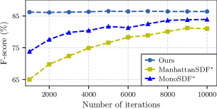
Figure 6: Ablation studies on the number of training iterations for per-scene optimization.

Fast optimization. Our approach can achieve high-quality reconstruction at approximately 1.5K iterations within 15 minutes. As illustrated in Fig. 6, our method achieves a high F-score at the very early training stage, while Manhattan SDF^∗ (Guo et al., 2022) and MonoSDF^∗ (Yu et al., 2022) take much more iterations to reach a similar performance.

5 Conclusion

In this work, we present a generalizable scene prior that enables fast, large-scale scene reconstruction of geometry and texture. Our model follows a single-view RGB-D input setting and allows non-learnable direct fusion of images. We design a two-stage paradigm to learn the generalizable geometric and texture networks. Large-scale, high-fidelity scene reconstruction can be obtained with efficient fine-tuning on the pretrained scene priors, even with limited views. We demonstrate that our approach can achieve state-of-the-art quality of indoor scene reconstruction with fine geometric details and realistic texture.

References

- Azinović et al. (2022) Dejan Azinović, Ricardo Martin-Brualla, Dan B Goldman, Matthias Nießner, and Justus Thies. Neural rgb-d surface reconstruction. In Proceedings of the IEEE/CVF Conference on Computer Vision and Pattern Recognition, pp. 6290–6301, 2022.
- Bi et al. (2017) Sai Bi, Nima Khademi Kalantari, and Ravi Ramamoorthi. Patch-based optimization for image-based texture mapping. ACM Trans. Graph., 36(4):106–1, 2017.
- Chen et al. (2021) Anpei Chen, Zexiang Xu, Fuqiang Zhao, Xiaoshuai Zhang, Fanbo Xiang, Jingyi Yu, and Hao Su. Mvsnerf: Fast generalizable radiance field reconstruction from multi-view stereo. In Proceedings of the IEEE/CVF International Conference on Computer Vision, pp. 14124–14133, 2021.
- Cheng et al. (2020) Shuo Cheng, Zexiang Xu, Shilin Zhu, Zhuwen Li, Li Erran Li, Ravi Ramamoorthi, and Hao Su. Deep stereo using adaptive thin volume representation with uncertainty awareness. In Proceedings of the IEEE/CVF Conference on Computer Vision and Pattern Recognition, pp. 2524–2534, 2020.
- Dai et al. (2017a) Angela Dai, Angel X Chang, Manolis Savva, Maciej Halber, Thomas Funkhouser, and Matthias Nießner. Scannet: Richly-annotated 3d reconstructions of indoor scenes. In CVPR, pp. 5828–5839, 2017a.
- Dai et al. (2017b) Angela Dai, Matthias Nießner, Michael Zollhöfer, Shahram Izadi, and Christian Theobalt. Bundlefusion: Real-time globally consistent 3d reconstruction using on-the-fly surface reintegration. ACM Transactions on Graphics (ToG), 36(4):1, 2017b.
- Deng et al. (2022) Kangle Deng, Andrew Liu, Jun-Yan Zhu, and Deva Ramanan. Depth-supervised nerf: Fewer views and faster training for free. In Proceedings of the IEEE/CVF Conference on Computer Vision and Pattern Recognition, pp. 12882–12891, 2022.
- Düzçeker et al. (2020) Arda Düzçeker, Silvano Galliani, Christoph Vogel, Pablo Speciale, Mihai Dusmanu, and Marc Pollefeys. DeepVideoMVS: Multi-View Stereo on Video with Recurrent Spatio-Temporal Fusion. arXiv preprint arXiv:2012.02177, 2020.
- Guo et al. (2022) Haoyu Guo, Sida Peng, Haotong Lin, Qianqian Wang, Guofeng Zhang, Hujun Bao, and Xiaowei Zhou. Neural 3d scene reconstruction with the manhattan-world assumption. In Proceedings of the IEEE/CVF Conference on Computer Vision and Pattern Recognition, pp. 5511–5520, 2022.
- He et al. (2016) Kaiming He, Xiangyu Zhang, Shaoqing Ren, and Jian Sun. Deep residual learning for image recognition. In Proceedings of the IEEE conference on computer vision and pattern recognition, pp. 770–778, 2016.
- Huang et al. (2021) Jiahui Huang, Shi-Sheng Huang, Haoxuan Song, and Shi-Min Hu. Di-fusion: Online implicit 3d reconstruction with deep priors. In Proceedings of the IEEE/CVF Conference on Computer Vision and Pattern Recognition, pp. 8932–8941, 2021.
- Huang et al. (2018) Po-Han Huang, Kevin Matzen, Johannes Kopf, Narendra Ahuja, and Jia-Bin Huang. Deepmvs: Learning multi-view stereopsis. In Proceedings of the IEEE Conference on Computer Vision and Pattern Recognition, pp. 2821–2830, 2018.
- Johari et al. (2022) Mohammad Mahdi Johari, Yann Lepoittevin, and François Fleuret. Geonerf: Generalizing nerf with geometry priors. In Proceedings of the IEEE/CVF Conference on Computer Vision and Pattern Recognition, pp. 18365–18375, 2022.
- Li et al. (2022) Kejie Li, Yansong Tang, Victor Adrian Prisacariu, and Philip HS Torr. Bnv-fusion: Dense 3d reconstruction using bi-level neural volume fusion. In Proceedings of the IEEE/CVF Conference on Computer Vision and Pattern Recognition, pp. 6166–6175, 2022.
- Liang et al. (2023) Zhihao Liang, Zhangjin Huang, Changxing Ding, and Kui Jia. Helixsurf: A robust and efficient neural implicit surface learning of indoor scenes with iterative intertwined regularization. In Proceedings of the IEEE/CVF Conference on Computer Vision and Pattern Recognition, pp. 13165–13174, 2023.
- Liu et al. (2020) Lingjie Liu, Jiatao Gu, Kyaw Zaw Lin, Tat-Seng Chua, and Christian Theobalt. Neural sparse voxel fields. In NeurIPS, 2020.
- Long et al. (2022) Xiaoxiao Long, Cheng Lin, Peng Wang, Taku Komura, and Wenping Wang. Sparseneus: Fast generalizable neural surface reconstruction from sparse views. arXiv preprint arXiv:2206.05737, 2022.
- Luo et al. (2019) Keyang Luo, Tao Guan, Lili Ju, Haipeng Huang, and Yawei Luo. P-mvsnet: Learning patch-wise matching confidence aggregation for multi-view stereo. In Proceedings of the IEEE/CVF International Conference on Computer Vision, pp. 10452–10461, 2019.
- Merrell et al. (2007) Paul Merrell, Amir Akbarzadeh, Liang Wang, Philippos Mordohai, Jan-Michael Frahm, Ruigang Yang, David Nistér, and Marc Pollefeys. Real-time visibility-based fusion of depth maps. In 2007 IEEE 11th International Conference on Computer Vision, pp. 1–8. Ieee, 2007.
- Mildenhall et al. (2020) Ben Mildenhall, Pratul P Srinivasan, Matthew Tancik, Jonathan T Barron, Ravi Ramamoorthi, and Ren Ng. NeRF: Representing Scenes as Neural Radiance Fields for View Synthesis. In ECCV, pp. 405–421. Springer, 2020.
- Newcombe et al. (2011) Richard A Newcombe, Shahram Izadi, Otmar Hilliges, David Molyneaux, David Kim, Andrew J Davison, Pushmeet Kohi, Jamie Shotton, Steve Hodges, and Andrew Fitzgibbon. Kinectfusion: Real-time dense surface mapping and tracking. In 2011 10th IEEE international symposium on mixed and augmented reality, pp. 127–136. Ieee, 2011.
- Niemeyer et al. (2020) Michael Niemeyer, Lars Mescheder, Michael Oechsle, and Andreas Geiger. Differentiable volumetric rendering: Learning implicit 3d representations without 3d supervision. In CVPR, pp. 3504–3515, 2020.
- Nowacki & Woda (2019) Paweł Nowacki and Marek Woda. Capabilities of arcore and arkit platforms for ar/vr applications. In International Conference on Dependability and Complex Systems, pp. 358–370. Springer, 2019.
- Oechsle et al. (2021) Michael Oechsle, Songyou Peng, and Andreas Geiger. Unisurf: Unifying neural implicit surfaces and radiance fields for multi-view reconstruction. In Proceedings of the IEEE/CVF International Conference on Computer Vision, pp. 5589–5599, 2021.
- Ortiz et al. (2022) Joseph Ortiz, Alexander Clegg, Jing Dong, Edgar Sucar, David Novotny, Michael Zollhoefer, and Mustafa Mukadam. isdf: Real-time neural signed distance fields for robot perception. arXiv preprint arXiv:2204.02296, 2022.
- Peng et al. (2020) Songyou Peng, Michael Niemeyer, Lars Mescheder, Marc Pollefeys, and Andreas Geiger. Convolutional occupancy networks. In European Conference on Computer Vision, pp. 523–540. Springer, 2020.
- Ronneberger et al. (2015) Olaf Ronneberger, Philipp Fischer, and Thomas Brox. U-net: Convolutional networks for biomedical image segmentation. In International Conference on Medical image computing and computer-assisted intervention, pp. 234–241. Springer, 2015.
- Schonberger & Frahm (2016) Johannes L Schonberger and Jan-Michael Frahm. Structure-from-motion revisited. In CVPR, pp. 4104–4113, 2016.
- Schönberger et al. (2016) Johannes L Schönberger, Enliang Zheng, Jan-Michael Frahm, and Marc Pollefeys. Pixelwise view selection for unstructured multi-view stereo. In ECCV, pp. 501–518. Springer, 2016.
- Sitzmann et al. (2020) Vincent Sitzmann, Julien Martel, Alexander Bergman, David Lindell, and Gordon Wetzstein. Implicit neural representations with periodic activation functions. Advances in Neural Information Processing Systems, 33:7462–7473, 2020.
- Smisek et al. (2013) Jan Smisek, Michal Jancosek, and Tomas Pajdla. 3d with kinect. In Consumer depth cameras for computer vision, pp. 3–25. Springer, 2013.
- Sucar et al. (2021) Edgar Sucar, Shikun Liu, Joseph Ortiz, and Andrew J Davison. imap: Implicit mapping and positioning in real-time. In Proceedings of the IEEE/CVF International Conference on Computer Vision, pp. 6229–6238, 2021.
- Sun et al. (2022a) Cheng Sun, Min Sun, and Hwann-Tzong Chen. Direct voxel grid optimization: Super-fast convergence for radiance fields reconstruction. In CVPR, 2022a.
- Sun et al. (2022b) Cheng Sun, Min Sun, and Hwann-Tzong Chen. Direct voxel grid optimization: Super-fast convergence for radiance fields reconstruction. In Proceedings of the IEEE/CVF Conference on Computer Vision and Pattern Recognition, pp. 5459–5469, 2022b.
- Sun et al. (2021) Jiaming Sun, Yiming Xie, Linghao Chen, Xiaowei Zhou, and Hujun Bao. Neuralrecon: Real-time coherent 3d reconstruction from monocular video. In Proceedings of the IEEE/CVF Conference on Computer Vision and Pattern Recognition, pp. 15598–15607, 2021.
- Takikawa et al. (2021) Towaki Takikawa, Joey Litalien, Kangxue Yin, Karsten Kreis, Charles Loop, Derek Nowrouzezahrai, Alec Jacobson, Morgan McGuire, and Sanja Fidler. Neural geometric level of detail: Real-time rendering with implicit 3d shapes. In Proceedings of the IEEE/CVF Conference on Computer Vision and Pattern Recognition, pp. 11358–11367, 2021.
- Wang et al. (2022a) Jiepeng Wang, Peng Wang, Xiaoxiao Long, Christian Theobalt, Taku Komura, Lingjie Liu, and Wenping Wang. Neuris: Neural reconstruction of indoor scenes using normal priors. In European Conference on Computer Vision, pp. 139–155. Springer, 2022a.
- Wang et al. (2022b) Jingwen Wang, Tymoteusz Bleja, and Lourdes Agapito. Go-surf: Neural feature grid optimization for fast, high-fidelity rgb-d surface reconstruction. arXiv preprint arXiv:2206.14735, 2022b.
- Wang et al. (2021a) Peng Wang, Lingjie Liu, Yuan Liu, Christian Theobalt, Taku Komura, and Wenping Wang. Neus: Learning neural implicit surfaces by volume rendering for multi-view reconstruction. arXiv preprint arXiv:2106.10689, 2021a.
- Wang et al. (2021b) Qianqian Wang, Zhicheng Wang, Kyle Genova, Pratul P Srinivasan, Howard Zhou, Jonathan T Barron, Ricardo Martin-Brualla, Noah Snavely, and Thomas Funkhouser. Ibrnet: Learning multi-view image-based rendering. In Proceedings of the IEEE/CVF Conference on Computer Vision and Pattern Recognition, pp. 4690–4699, 2021b.
- Wei et al. (2021) Yi Wei, Shaohui Liu, Yongming Rao, Wang Zhao, Jiwen Lu, and Jie Zhou. Nerfingmvs: Guided optimization of neural radiance fields for indoor multi-view stereo. In Proceedings of the IEEE/CVF International Conference on Computer Vision, pp. 5610–5619, 2021.
- Williams et al. (2022) Francis Williams, Zan Gojcic, Sameh Khamis, Denis Zorin, Joan Bruna, Sanja Fidler, and Or Litany. Neural fields as learnable kernels for 3d reconstruction. In Proceedings of the IEEE/CVF Conference on Computer Vision and Pattern Recognition, pp. 18500–18510, 2022.
- Wu et al. (2019) Wenxuan Wu, Zhongang Qi, and Li Fuxin. Pointconv: Deep convolutional networks on 3d point clouds. In Proceedings of the IEEE/CVF Conference on Computer Vision and Pattern Recognition, pp. 9621–9630, 2019.
- Xu et al. (2022) Qiangeng Xu, Zexiang Xu, Julien Philip, Sai Bi, Zhixin Shu, Kalyan Sunkavalli, and Ulrich Neumann. Point-nerf: Point-based neural radiance fields. In Proceedings of the IEEE/CVF Conference on Computer Vision and Pattern Recognition, pp. 5438–5448, 2022.
- Yao et al. (2018) Yao Yao, Zixin Luo, Shiwei Li, Tian Fang, and Long Quan. Mvsnet: Depth inference for unstructured multi-view stereo. In Proceedings of the European conference on computer vision (ECCV), pp. 767–783, 2018.
- Yariv et al. (2020) Lior Yariv, Yoni Kasten, Dror Moran, Meirav Galun, Matan Atzmon, Basri Ronen, and Yaron Lipman. Multiview neural surface reconstruction by disentangling geometry and appearance. Advances in Neural Information Processing Systems, 33:2492–2502, 2020.
- Yariv et al. (2021) Lior Yariv, Jiatao Gu, Yoni Kasten, and Yaron Lipman. Volume rendering of neural implicit surfaces. Advances in Neural Information Processing Systems, 34:4805–4815, 2021.
- Yen-Chen et al. (2020) Lin Yen-Chen, Pete Florence, Jonathan T Barron, Alberto Rodriguez, Phillip Isola, and Tsung-Yi Lin. iNeRF: Inverting Neural Radiance Fields for Pose Estimation. arXiv preprint arXiv:2012.05877, 2020.
- Yu et al. (2022) Zehao Yu, Songyou Peng, Michael Niemeyer, Torsten Sattler, and Andreas Geiger. Monosdf: Exploring monocular geometric cues for neural implicit surface reconstruction. arXiv preprint arXiv:2206.00665, 2022.
- Zhang et al. (2020) Kai Zhang, Gernot Riegler, Noah Snavely, and Vladlen Koltun. Nerf++: Analyzing and improving neural radiance fields. arXiv preprint arXiv:2010.07492, 2020.
- Zhang et al. (2022) Xiaoshuai Zhang, Sai Bi, Kalyan Sunkavalli, Hao Su, and Zexiang Xu. Nerfusion: Fusing radiance fields for large-scale scene reconstruction. In Proceedings of the IEEE/CVF Conference on Computer Vision and Pattern Recognition, pp. 5449–5458, 2022.
- Zhang (2012) Zhengyou Zhang. Microsoft kinect sensor and its effect. IEEE multimedia, 19(2):4–10, 2012.
- Zhou et al. (2018) Qian-Yi Zhou, Jaesik Park, and Vladlen Koltun. Open3d: A modern library for 3d data processing. arXiv preprint arXiv:1801.09847, 2018.
- Zhu et al. (2022) Zihan Zhu, Songyou Peng, Viktor Larsson, Weiwei Xu, Hujun Bao, Zhaopeng Cui, Martin R Oswald, and Marc Pollefeys. Nice-slam: Neural implicit scalable encoding for slam. In Proceedings of the IEEE/CVF Conference on Computer Vision and Pattern Recognition, pp. 12786–12796, 2022.