D-64289 Darmstadt, Germanybbinstitutetext: ExtreMe Matter Institute EMMI, GSI Helmholtzzentrum für Schwerionenforschung GmbH, 64291 Darmstadt, Germany
Bounding the QCD Equation of State with the Lattice
Abstract
The equation of state of QCD matter at high densities is relevant for neutron star structure and for neutron star mergers and has been a focus of recent work. We show how lattice QCD simulations, free of sign problems, can provide an upper bound on the pressure as a function of quark chemical potentials. We show that at large chemical potentials this bound should become quite sharp; the difference between the upper bound on the pressure and the true pressure is of order . The corrections arise from a single Feynman diagram; its calculation would render remaining corrections .
Keywords:
Neutron star equation of state, lattice gauge theory1 Introduction
The equation of state (EOS) of strongly interacting matter dictates the thermodynamics of any system ultimately composed of quarks and gluons. At high temperatures and low net baryon densities, the EOS can be computed directly from the partition function of Quantum Chromodynamics (QCD) using Monte-Carlo lattice techniques Borsanyi:2013bia ; HotQCD:2014kol and compared to experimental determinations of thermodynamic properties Gardim:2019xjs . However, at low temperatures and high net baryon densities, such techniques fail due to the well-known sign problem deForcrand:2009zkb ; Nagata:2021ugx , and alternative methods are required to determine the EOS.
Such cold and dense QCD matter is in fact realized in nature in the cores of massive neutron stars, where matter is in equilibrium under the weak interactions (beta equilibrated) and dense enough to populate the three lightest quark flavors. In this context, the EOS is intimately tied to the bulk properties of neutron stars via the stellar structure equations of general relativity Tolman:1939jz ; Oppenheimer:1939ne , and hence observations of neutron star properties, such as masses Antoniadis:2013pzd ; Cromartie:2019kug ; Fonseca:2021wxt , tidal deformabilities TheLIGOScientific:2017qsa ; LIGOScientific:2018cki ; LIGOScientific:2018hze , and radii Steiner:2017vmg ; Nattila:2017wtj ; Shawn:2018 ; Miller:2019cac ; Riley:2019yda ; Miller:2021qha ; Riley:2021pdl can be used to constrain the EOS of QCD. Recently the community has converged on a strategy for inferring the EOS of cold and dense QCD matter using these astrophysical constraints in combination with a general set of causal extensions of low-density effective-field-theory calculations Tews:2012fj ; Lynn:2015jua ; Drischler:2017wtt ; Drischler:2020hwi ; Keller:2022crb of the EOS of dense nuclear matter (see, e.g., Hebeler:2013nza ; Tews:2018iwm ; Landry:2018prl ; Dietrich:2020efo ; Capano:2019eae ; Raaijmakers:2019dks ; Landry:2020vaw ; Essick:2019ldf ; Miller:2019nzo ; Al-Mamun:2020vzu ; Miller:2021qha ; Essick:2021kjb ; Huth:2021bsp ; Lim:2022fap ; Essick:2023fso ), sometimes also paired with constraints from perturbative QCD calculations at high net baryon densities Kurkela:2009gj ; Kurkela:2016was ; Gorda:2018gpy ; Gorda:2021znl ; Komoltsev:2021jzg ; Gorda:2021gha ; Gorda:2023mkk ; Gorda:2023usm (see, e.g. Kurkela:2014vha ; Annala:2017llu ; Most:2018hfd ; Altiparmak:2022bke ; Annala:2019puf ; Annala:2021gom ; Gorda:2022jvk ; Somasundaram:2022ztm ; Han:2022rug ; Jiang:2022tps ; Annala:2023cwx ; Brandes:2023hma ; Mroczek:2023zxo ). In addition to these constraints, there has been recent work on incorporating other experimental constraints, such as bounds from low-energy nuclear collision experiments Huth:2021bsp ; Sorensen:2023zkk , which have so far been seen to compliment those from astrophysics. On the theoretical side, the unitary gas constraint 2002PThPS.146..363C ; Schwenk:2005ka ; Carlson:2012mh ; Gandolfi:2015jma ; Tews:2016jhi – which has been conjectured to provide a lower bound of the energy per particle at low to moderate net baryon densities in the hadronic phase – has been used as a reference to benchmark different nuclear-theory calculations of the hadronic EOS as they are extended to higher densities.
In this paper we argue that one more constraint (or family of constraints) can be added to this list of bounds on the dense QCD EOS. While lattice QCD cannot compute the EOS for the physical combination of chemical potentials, phase-quenched lattice QCD is free of sign problems. The pressure as a function of chemical potentials, calculated using phase quenching, , is a strict upper bound on the true pressure at the same values of quark chemical potentials: . This fact was established by Cohen in Ref. Cohen:2003ut , who used it to show how the case of an isospin chemical potential – opposite up and down quark chemical potentials – can be used to bound the more physically interesting case of equal up and down quark chemical potentials. Unfortunately, the combination of chemical potentials relevant for neutron stars is rather different: the down and strange chemical potentials should be equal , while the up-quark chemical potential is somewhat smaller to accommodate charge neutrality, . Bounding the equation of state for this combination of chemical potentials starting from lattice results for isospin chemical potentials requires the use of additional inequalities Lee:2004hc , as recently explored by Fujimoto and Reddy Fujimoto:2023unl .
We argue here that the most effective way to use the lattice to bound the neutron-star equation of state is to perform new phase-quenched lattice simulations using the physical combination of up, down, and strange quark chemical potentials. Unlike an isospin chemical potential, the phase-quenched version of such a combination represents a completely unphysical system. But we expect that it will present the tightest bounds on the physical equation of state. In particular, we show here that, while at low densities the constraint is likely to be very loose, at high densities it should become ever sharper. In fact, we will demonstrate that, in the perturbative region, the relative difference is of order . Furthermore, at this order in the coupling expansion, the difference arises from a single Feynman diagram, which we identify.111Two diagrams if one considers the two directions which fermion arrows in a loop can point to represent distinct diagrams.
An outline of this paper is as follows. In the next section we review the path integral for QCD at finite chemical potential, and how it is related to the phase-quenched version. The section reviews the (quite simple) proof that , and discusses a little more how one should interpret the phase-quenched calculation. In Section 3 we show how to represent the (unphysical) phase-quenched theory in Feynman diagrams, and we identify the unique diagram which differs between and . Section 4 estimates the size of lattice artifacts in evaluating the pressure on the lattice, in order to give guidance for how small the lattice spacing must be at a given, large value. We end with a discussion, which lists the most important directions for further work.
2 Path integral and phase quenching
Here we review the proof that the pressure from the phase-quenched theory is a strict upper bound on the original theory. The proof as we formulate it is due to Cohen Cohen:2003ut , though the underlying ideas are older Alford:1998sd . The partition function of QCD at a small finite temperature in a box with a large volume and with quark chemical potentials is222The integral as written requires either gauge fixing or a restriction that should be understood only to run over distinct affine connections, but this point is not relevant here, since the fermionic determinants are our main focus.
| (1) |
Because and have different -Hermiticity deForcrand:2009zkb , each determinant is complex. Phase quenching is the replacement of with
| (2) |
That is, one uses the absolute values of the determinants, rather than the determinants themselves. Since the Euclidean gluonic action is strictly real,333We assume that the QCD theta angle tHooft:1976 ; Jackiw:1976pf ; Callan:1979bg is zero. the integrand is now real and positive and equals the absolute value of the integrand for . Since the integral of the absolute value of a function over a positive measure is greater than or equal to the integral of the original complex function, we have
| (3) |
where is the pressure.444In practice we want , that is, one should subtract the zero-chemical-potential value of the pressure. This has the benefit of removing cosmological-constant-type power UV divergences.
Let us investigate the interpretation of the phase-quenched theory. Applying -Hermiticity, one finds that Cohen:2003kd ; deForcrand:2009zkb
| (4) |
and therefore
| (5) | ||||
| (6) | ||||
Therefore, the phase-quenched theory is equivalent to a theory with twice as many fermionic species, but where each is represented by the square root of a determinant – think of each as a half-species, which appear in pairs with equal mass but opposite chemical potential. This theory is clearly unphysical, since a half-species of fermion does not make sense as an external state. A well known exception is if two quark masses and chemical potentials are equal Alford:1998sd ; Son:2000xc ; Son:2000by ; Splittorff:2000mm . In particular, for and with , representing “standard” baryonic chemical potential, the phase-quenched version is equivalent, after re-labeling two of the half-species, to the case , corresponding to an isospin chemical potential. This among other things has motivated rather detailed lattice investigations of the case of finite isospin chemical potential, see for instance Refs. Kogut:2002tm ; Kogut:2002zg ; Nishida:2003fb ; Kogut:2004zg ; Beane:2007es ; Detmold:2008fn ; Detmold:2012wc ; Endrodi:2014lja ; Janssen:2015lda ; Brandt:2017oyy ; Brandt:2019hel ; Brandt:2021yhc ; Brandt:2022hwy ; Abbott:2023coj or the comprehensive review by Mannarelli Mannarelli:2019hgn . In this case it is particularly clear that, for small chemical potentials, the two pressures are quite different. Tom Cohen has analyzed the case for an isospin chemical potential Cohen:2003kd and shown that nonzero in Eq. (5) does not change the value of the determinant until , when eigenvalues of start to cross the imaginary axis. He refers to the constancy of the determinant up to this point as “the silver blaze problem.” Applying his analysis for the general case of distinct , one finds that first deviates from its vacuum value when either , , or , where is the mass of the unphysical strange-antistrange pseudoscalar obtained by ignoring disconnected contributions to the correlation function. Therefore, at small chemical potentials , differs significantly from the physical pressure.
In the next section we will see that, for large chemical potentials, the two pressures become much more similar.
3 Perturbation theory
To construct a perturbation theory for Eq. (6), as usual for fermions, we rewrite
| (7) |
The process of deriving Feynman rules from is the same as without the factor, except that each fermionic loop receives a factor of . Therefore, in each place where a fermionic loop can appear, instead of performing a sum over fermions, each with mass and chemical potential , we sum over terms; twice for each , once with and once with but each with an overall factor of . This is the same as averaging the loop over whether is positive or negative.
To see the impact of we remind the reader about Furry’s theorem Furry:1937zz . Consider a fermion loop with external gluons connected by propagators, with incoming momenta with by momentum conservation. The fermions are in a representation (typically the fundamental representation) with Hermitian generators . Its group-theory factor and the numerator of its Feynman rule are
| (8) |
where is the loop momentum and . Inserting the charge conjugation matrix times its inverse, , between each neighboring term and using , we find
| (9) |
Reversing the order of the symbols to get rid of the transposes on the gamma matrices, and using for the Hermitian group generators, we find
| (10) |
which is the same diagram,555Reversing the sense in which the loop is traversed flips the signs of the momenta as well as reversing the order of the matrices in the color and Dirac traces. traversed in the opposite sense, with and with which is the generator of the conjugate representation – so if the generate the fundamental representation, the generate the antifundamental representation. Another way to state Furry’s theorem is then that reversing the sign of is equivalent to considering fermions with the original value but in the conjugate representation (quarks with are the same as antiquarks with ).
For the case of two external gluons we have
| (11) |
and the fundamental and antifundamental representations give the same answer. The representations first differ when there are three gluons attached:
| but | |||||
| (12) | |||||
where is a totally symmetric symbol which arises in groups of rank 2 or more.
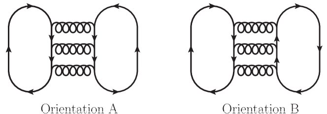
Because both and , the first group-theoretical structure where can give a nonzero contribution, for the group SU(), is
| (13) |
This contraction can only appear in a diagram with at least two fermion loops with at least three gluon attachments each. The only such diagram at the level is shown in Figure 1. Fermion number can traverse the two loops with two relative orientations, shown on the left and the right in the figure. We will write the two versions of the diagram, stripping off all group-theory factors, for two specific species , as and . That is, and represent the value of each fermion orientation in the abelian version of the diagram. In this notation, the contribution of this diagram to the true pressure is
| (14) |
In the abelian theory the group-theoretical coefficients on the first and second terms of the second line would be 1 and 0 respectively.
Furry’s Theorem means that . This allows us to rewrite Eq. (3) in terms of only:
| (15) |
Averaging over and/or , as we are instructed to do in evaluating , eliminates the first expression and leaves only the second. Therefore, the difference between the phase-quenched and true pressure, at order , is
| (16) |
We can show that this combination is automatically positive; the proof, along with an explicit evaluation, will appear in a forthcoming publication.
Evaluating this single combination of diagrams would determine the perturbative correction between the phase-quenched and true pressures, through to order . Any quark with does not contribute to Eq. (16). The contribution of soft gluon momenta to Eq. (16) is suppressed, since the three-gluon hard loop contains only the group-theory factor Braaten:1989mz .666We are indebted to Saga Säppi for useful conversations on this point. Therefore Eq. (16) does not contain any logarithmically enhanced contributions.
As an aside, we comment on the behavior of these terms as a function of . In the large or t’Hooft limit, the group-theory factor on Orientation in Eq. (3) is while that for Orientation is and is suppressed. In contrast, for the group SU(2), the group-theoretical factor on in Eq. (3) vanishes and there is no distinction between the fundamental and antifundamental representations. In fact, because every SU(2) representation is equivalent to its conjugate representation, it is easy to show that any combination of chemical potentials is free of sign problems in 2-color QCD, which has motivated investigation of this theory at finite density Kogut:1999iv ; Kogut:2000ek ; Cotter:2012mb ; Astrakhantsev:2020tdl ; Boz:2019enj ; Iida:2022hyy ; Braguta:2023yhd .
4 Lattice considerations
The previous sections have made clear that a lattice calculation of would be valuable. Here we want to take one small step towards estimating how difficult such a lattice calculation would be. The larger is, the more rapidly a lattice calculation develops statistical power; since , we expect that the signal-to-noise should scale roughly as . Therefore it is advantageous to work on lattices with the largest we can get away with.
But increasing increases systematic lattice-spacing effects. In general, for a lattice calculation to be accurate we need the lattice spacing to obey . But introduces an additional scale, and for the regime , we expect to need the stronger condition . But what does really mean – that is, how small does really need to be? To estimate this, we compute how different the vacuum-subtracted777The pressure receives divergent vacuum contributions (the cosmological constant problem) which have to be subtracted in a lattice treatment. pressure is on the lattice from its continuum value, at lowest (zero) order in the strong coupling. Here we will only consider staggered quarks Kogut:1974ag ; Banks:1975gq ; Susskind:1976jm , since we expect this quark formulation to be used in practical calculations.
In the continuum, one free Dirac fermion with chemical potential provides a pressure of
| (17) |
where the second term subtracts the “vacuum” pressure. Evaluating the trace, one finds
| (18) |
Naively it appears that contributes to the pressure at any value including when , but this is illusory. Separating the numerator and denominator of the log, one may deform the integration contour for the former, shifting it by . If then this contour deformation encounters no singularities, and the integral at nonzero and at zero are identical. For there is a cut running from to with discontinuity which the deformed contour must enclose, leading to
| (19) |
as expected. The expressions for the energy density and for the chemical potential times the number density are the same but with the first factor, , replaced by and by respectively, recovering the thermodynamical relation .
Naive staggered fermions Susskind:1976jm represent four species of physical fermions with the limitation that each component runs over with the lattice spacing888The Brillouin zone should run over but it is divided into 16 regions in which each component of runs over half as large a range, . These regions represent 16 “doubler” fermions, and the staggering procedure removes a factor of 4. For a review see Gattringer:2010zz . and with the substitution
| (20) |
Here and represent the unit vector in the spatial direction and in the time direction respectively. Note that the effects of must be incorporated along with the time derivative because, in the staggered formulation, an insertion of requires that the comparison be made between and which differ by an odd number of steps in the time direction. This is in any case the preferred way of introducing a chemical potential because it avoids quadratic-in- lattice artifacts, see Hasenfratz:1983ba . The fact that a staggered fermion represents four physical fermions is handled through the fourth-root trick and leads to a pressure for one physical fermion of
| (21) |
There are two effects. First, the lattice, rather than physical, dispersion determines the energy . Second, the range is finite and periodic and appears inside a trigonometric function inside the log. Nevertheless, a contour deformation, , is still possible, and it encounters a similar discontinuity in the log:
| (22) |
We have only been able to compute the resulting integral numerically, but as expected, the leading small- corrections are of order . Specifically, the flatter dispersion relation lowers and leads to a larger phase space region where fermionic states are occupied.
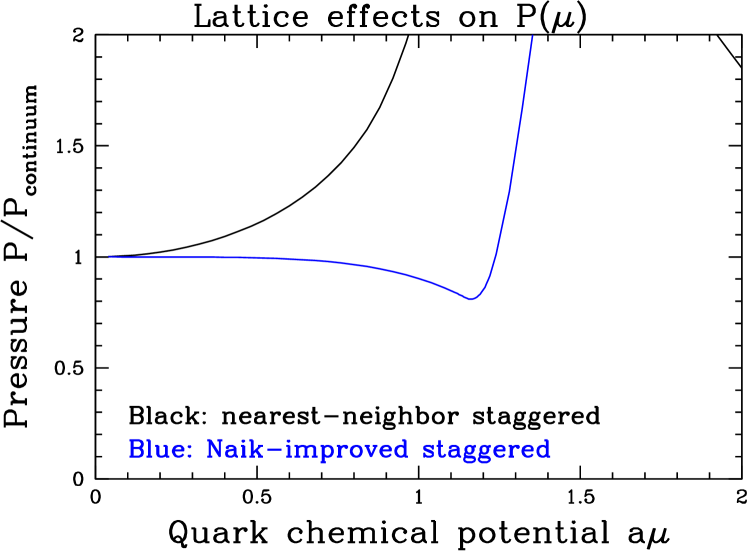
We show the results of a simple numerical evaluation of Eq. (22) in Figure 2. We have also checked that carrying out the integral shown in Eq. (4) leads to the same result. Unfortunately, if we set as a criterion for good convergence that the lattice and continuum pressures should differ by at most 10%, we are restricted to . To do better, we could use an improved fermionic action. Naik has advocated Naik:1986bn that one replace Eq. (4) with an improved version,
| (23) |
As shown in Figure 2, this dramatically improves the match between the lattice and continuum pressure, such that still has corrections. However, beyond , and the “improvement” term in Eq. (4) starts to dominate over the nearest-neighbor term. This leads to additional cuts in the modified version of Eq. (4), and the performance of this implementation rather abruptly breaks down.
With these results in mind, we feel that nearest-neighbor staggered quarks can only treat large accurately out to disappointingly small or 0.5 – possibly a little higher with the help of extrapolation over a few lattice spacings. Improved quarks, such as ASQTAD Orginos:1998ue ; Lepage:1998vj or HISQ Follana:2006rc quarks, which use the Naik term, should be able to do better but it is very dangerous to venture beyond .
Another limitation of a lattice treatment is that one generically must compute at finite temperature. Therefore we should also estimate the size of thermal effects. We will assume that the thermal corrections are similar to those in the continuum. At the free theory level, the pressure of a single Dirac fermion with chemical potential at temperature actually has a closed form:
| (24) |
This implies to keep thermal effects at the 10% level.
One can attempt to remove both lattice-spacing and temperature effects through extrapolation over multiple lattice spacings and box sizes. In the case of lattice spacing effects, an effective field theory analysis at the scale tells us that the lattice-spacing effects should scale as up to anomalous dimension corrections. The coefficient will not necessarily equal the free-theory one, but the effect should definitely be a power law with power close to 2. More care is needed in extrapolating away temperature effects. While one might expect that the leading thermal effects are of order as in Eq. (24), this is really an assumption which can go wrong if, for instance, the theory develops a mass gap due to interactions between excitations near the Fermi surface. Therefore we expect that more care must be taken when extrapolating to small temperature.
5 Discussion
This paper has made three points.
-
•
Lattice QCD can study arbitrary combinations of using phase-quenching, providing . Though this does not return the true QCD pressure, it returns a strict upper bound on the true pressure: , which could still be useful in constraining the equation of state for neutron star matter.
-
•
The difference is small at weak coupling, in the sense that . Furthermore, the contribution arises from a single diagram. If we could compute this diagram, we could use to determine up to corrections (up to logs and nonperturbative effects such as pairing gaps).
-
•
Lattice calculations of encounter lattice artifacts. We estimate the size of these artifacts and advocate that nearest-neighbor fermion formulations use , while improved-dispersion fermions may be reliable at chemical potentials more than a factor of 2 larger.
The first step in utilizing this approach is to perform a lattice study at a series of chemical potentials. For neutron star physics one should choose and somewhat smaller to describe a charge-neutral system including equilibrated leptons. One might study a range of chemical potentials from MeV to 1 GeV. Since a lattice approach will likely involve determining at each value and integrating it to find the pressure using , it appears necessary to consider a tightly spaced series of values. One also needs a few lattice spacings in order to perform a continuum extrapolation.
The next step would be to use these values as constraints, when considering the high-density QCD equation of state. A proposed QCD equation of state is usually expressed as a curve in either the , , or plane. Standard thermodynamical relations can convert this into a curve in the plane; if the proposed EOS exceeds for any where we have data, it is excluded.
Next, the possibility of evaluating directly on the lattice at large can be used as a check on the performance of the perturbative expansion. Specifically, one can consider the perturbative expansion for , which as we have argued is the same as the expansion for at the currently known order of Gorda:2023mkk . By comparing this result to the lattice-determined , one can assess how accurate the perturbative series is as a function of the scale .
Finally, one should perform an accurate evaluation of the single diagram which introduces differences between and . In any -region where the result is actually a small correction, this can be used together with a lattice-determined to provide an improved estimate of . The resulting estimate would also be perturbatively complete at , with only , higher-order, and nonperturbative corrections remaining.
Acknowledgments
We would like to thank Gergely Endrődi and Saga Säppi for useful discussions. We acknowledge support by the Deutsche Forschungsgemeinschaft (DFG, German Research Foundation) through the CRC-TR 211 “Strong-interaction matter under extreme conditions”– project number 315477589 – TRR 211, the DFG-Project ID 279384907–SFB 1245, and by the State of Hesse within the Research Cluster ELEMENTS (Project ID 500/10.006).
References
- (1) S. Borsanyi, Z. Fodor, C. Hoelbling, S.D. Katz, S. Krieg and K.K. Szabo, Full result for the QCD equation of state with 2+1 flavors, Phys. Lett. B 730 (2014) 99 [1309.5258].
- (2) HotQCD collaboration, Equation of state in ( 2+1 )-flavor QCD, Phys. Rev. D 90 (2014) 094503 [1407.6387].
- (3) F.G. Gardim, G. Giacalone, M. Luzum and J.-Y. Ollitrault, Thermodynamics of hot strong-interaction matter from ultrarelativistic nuclear collisions, Nature Phys. 16 (2020) 615 [1908.09728].
- (4) P. de Forcrand, Simulating QCD at finite density, PoS LAT2009 (2009) 010 [1005.0539].
- (5) K. Nagata, Finite-density lattice QCD and sign problem: Current status and open problems, Prog. Part. Nucl. Phys. 127 (2022) 103991 [2108.12423].
- (6) R.C. Tolman, Static solutions of Einstein’s field equations for spheres of fluid, Phys. Rev. 55 (1939) 364.
- (7) J.R. Oppenheimer and G.M. Volkoff, On massive neutron cores, Phys. Rev. 55 (1939) 374.
- (8) J. Antoniadis, P.C.C. Freire, N. Wex, T.M. Tauris, R.S. Lynch, M.H. van Kerkwijk et al., A Massive Pulsar in a Compact Relativistic Binary, Science 340 (2013) 1233232 [https://www.science.org/doi/pdf/10.1126/science.1233232].
- (9) NANOGrav collaboration, Relativistic Shapiro delay measurements of an extremely massive millisecond pulsar, Nature Astron. 4 (2019) 72 [1904.06759].
- (10) E. Fonseca, H.T. Cromartie, T.T. Pennucci, P.S. Ray, A.Y. Kirichenko, S.M. Ransom et al., Refined Mass and Geometric Measurements of the High-mass PSR J0740+6620, Astrophys. J. Lett. 915 (2021) L12.
- (11) LIGO Scientific Collaboration and Virgo Collaboration collaboration, GW170817: Observation of Gravitational Waves from a Binary Neutron Star Inspiral, Phys. Rev. Lett. 119 (2017) 161101.
- (12) The LIGO Scientific Collaboration and the Virgo Collaboration collaboration, GW170817: Measurements of Neutron Star Radii and Equation of State, Phys. Rev. Lett. 121 (2018) 161101.
- (13) LIGO Scientific Collaboration and Virgo Collaboration collaboration, Properties of the Binary Neutron Star Merger GW170817, Phys. Rev. X 9 (2019) 011001.
- (14) A.W. Steiner, C.O. Heinke, S. Bogdanov, C. Li, W.C.G. Ho, A. Bahramian et al., Constraining the Mass and Radius of Neutron Stars in Globular Clusters, Mon. Not. Roy. Astron. Soc. 476 (2018) 421 [1709.05013].
- (15) J. Nättilä, M.C. Miller, A.W. Steiner, J.J.E. Kajava, V.F. Suleimanov and J. Poutanen, Neutron star mass and radius measurements from atmospheric model fits to X-ray burst cooling tail spectra, Astron. Astrophys. 608 (2017) A31 [1709.09120].
- (16) A.W. Shaw, C.O. Heinke, A.W. Steiner, S. Campana, H.N. Cohn, W.C.G. Ho et al., The radius of the quiescent neutron star in the globular cluster M13, Mon. Not. R. Astron. Soc. 476 (2018) 4713 [1803.00029].
- (17) M.C. Miller, F.K. Lamb, A.J. Dittmann, S. Bogdanov, Z. Arzoumanian, K.C. Gendreau et al., PSR J0030+0451 Mass and Radius from NICER Data and Implications for the Properties of Neutron Star Matter, Astrophys. J. Lett. 887 (2019) L24.
- (18) T.E. Riley, A.L. Watts, S. Bogdanov, P.S. Ray, R.M. Ludlam, S. Guillot et al., A NICER View of PSR J0030+0451: Millisecond Pulsar Parameter Estimation, Astrophys. J. Lett. 887 (2019) L21.
- (19) M.C. Miller, F.K. Lamb, A.J. Dittmann, S. Bogdanov, Z. Arzoumanian, K.C. Gendreau et al., The Radius of PSR J0740+6620 from NICER and XMM-Newton Data, Astrophys. J. Lett. 918 (2021) L28.
- (20) T.E. Riley, A.L. Watts, P.S. Ray, S. Bogdanov, S. Guillot, S.M. Morsink et al., A NICER View of the Massive Pulsar PSR J0740+6620 Informed by Radio Timing and XMM-Newton Spectroscopy, Astrophys. J. Lett. 918 (2021) L27.
- (21) I. Tews, T. Krüger, K. Hebeler and A. Schwenk, Neutron matter at next-to-next-to-next-to-leading order in chiral effective field theory, Phys. Rev. Lett. 110 (2013) 032504 [1206.0025].
- (22) J.E. Lynn, I. Tews, J. Carlson, S. Gandolfi, A. Gezerlis, K.E. Schmidt et al., Chiral Three-Nucleon Interactions in Light Nuclei, Neutron- Scattering, and Neutron Matter, Phys. Rev. Lett. 116 (2016) 062501 [1509.03470].
- (23) C. Drischler, K. Hebeler and A. Schwenk, Chiral interactions up to next-to-next-to-next-to-leading order and nuclear saturation, Phys. Rev. Lett. 122 (2019) 042501 [1710.08220].
- (24) C. Drischler, R.J. Furnstahl, J.A. Melendez and D.R. Phillips, How Well Do We Know the Neutron-Matter Equation of State at the Densities Inside Neutron Stars? A Bayesian Approach with Correlated Uncertainties, Phys. Rev. Lett. 125 (2020) 202702 [2004.07232].
- (25) J. Keller, K. Hebeler and A. Schwenk, Nuclear Equation of State for Arbitrary Proton Fraction and Temperature Based on Chiral Effective Field Theory and a Gaussian Process Emulator, Phys. Rev. Lett. 130 (2023) 072701 [2204.14016].
- (26) K. Hebeler, J.M. Lattimer, C.J. Pethick and A. Schwenk, Equation of state and neutron star properties constrained by nuclear physics and observation, Astrophys. J. 773 (2013) 11 [1303.4662].
- (27) I. Tews, J. Margueron and S. Reddy, Critical examination of constraints on the equation of state of dense matter obtained from GW170817, Phys. Rev. C 98 (2018) 045804 [1804.02783].
- (28) P. Landry and R. Essick, Nonparametric inference of the neutron star equation of state from gravitational wave observations, Phys. Rev. D 99 (2019) 084049 [1811.12529].
- (29) T. Dietrich, M.W. Coughlin, P.T.H. Pang, M. Bulla, J. Heinzel, L. Issa et al., Multimessenger constraints on the neutron-star equation of state and the Hubble constant, Science 370 (2020) 1450 [2002.11355].
- (30) C.D. Capano, I. Tews, S.M. Brown, B. Margalit, S. De, S. Kumar et al., Stringent constraints on neutron-star radii from multimessenger observations and nuclear theory, Nat. Astron. 4 (2020) 625 [1908.10352].
- (31) G. Raaijmakers, S.K. Greif, T.E. Riley et al., Constraining the dense matter equation of state with joint analysis of NICER and LIGO/Virgo measurements, Astrophys. J. Lett. 893 (2020) L21 [1912.11031].
- (32) P. Landry, R. Essick and K. Chatziioannou, Nonparametric constraints on neutron star matter with existing and upcoming gravitational wave and pulsar observations, Phys. Rev. D 101 (2020) 123007 [2003.04880].
- (33) R. Essick, P. Landry and D.E. Holz, Nonparametric Inference of Neutron Star Composition, Equation of State, and Maximum Mass with GW170817, Phys. Rev. D 101 (2020) 063007 [1910.09740].
- (34) M.C. Miller, C. Chirenti and F.K. Lamb, Constraining the equation of state of high-density cold matter using nuclear and astronomical measurements, Astrophys. J. 888 (2020) 12 [1904.08907].
- (35) M. Al-Mamun, A.W. Steiner, J. Nättilä, J. Lange, R. O’Shaughnessy, I. Tews et al., Combining Electromagnetic and Gravitational-Wave Constraints on Neutron-Star Masses and Radii, Phys. Rev. Lett. 126 (2021) 061101 [2008.12817].
- (36) R. Essick, I. Tews, P. Landry and A. Schwenk, Astrophysical Constraints on the Symmetry Energy and the Neutron Skin of Pb208 with Minimal Modeling Assumptions, Phys. Rev. Lett. 127 (2021) 192701 [2102.10074].
- (37) S. Huth et al., Constraining Neutron-Star Matter with Microscopic and Macroscopic Collisions, Nature 606 (2022) 276 [2107.06229].
- (38) Y. Lim and J.W. Holt, Neutron Star Radii, Deformabilities, and Moments of Inertia from Experimental and Ab Initio Theory Constraints of the 208Pb Neutron Skin Thickness, Galaxies 10 (2022) 99 [2204.09000].
- (39) R. Essick, I. Legred, K. Chatziioannou, S. Han and P. Landry, Phase transition phenomenology with nonparametric representations of the neutron star equation of state, Phys. Rev. D 108 (2023) 043013 [2305.07411].
- (40) A. Kurkela, P. Romatschke and A. Vuorinen, Cold Quark Matter, Phys. Rev. D 81 (2010) 105021 [0912.1856].
- (41) A. Kurkela and A. Vuorinen, Cool quark matter, Phys. Rev. Lett. 117 (2016) 042501 [1603.00750].
- (42) T. Gorda, A. Kurkela, P. Romatschke, S. Säppi and A. Vuorinen, Next-to-Next-to-Next-to-Leading Order Pressure of Cold Quark Matter: Leading Logarithm, Phys. Rev. Lett. 121 (2018) 202701 [1807.04120].
- (43) T. Gorda, A. Kurkela, R. Paatelainen, S. Säppi and A. Vuorinen, Soft Interactions in Cold Quark Matter, Phys. Rev. Lett. 127 (2021) 162003 [2103.05658].
- (44) O. Komoltsev and A. Kurkela, How Perturbative QCD Constrains the Equation of State at Neutron-Star Densities, Phys. Rev. Lett. 128 (2022) 202701 [2111.05350].
- (45) T. Gorda and S. Säppi, Cool quark matter with perturbative quark masses, Phys. Rev. D 105 (2022) 114005 [2112.11472].
- (46) T. Gorda, R. Paatelainen, S. Säppi and K. Seppänen, Equation of state of cold quark matter to , 2307.08734.
- (47) T. Gorda, O. Komoltsev, A. Kurkela and A. Mazeliauskas, Bayesian uncertainty quantification of perturbative QCD input to the neutron-star equation of state, JHEP 06 (2023) 002 [2303.02175].
- (48) A. Kurkela, E.S. Fraga, J. Schaffner-Bielich and A. Vuorinen, Constraining neutron star matter with Quantum Chromodynamics, Astrophys. J. 789 (2014) 127 [1402.6618].
- (49) E. Annala, T. Gorda, A. Kurkela and A. Vuorinen, Gravitational-wave constraints on the neutron-star-matter equation of state, Phys. Rev. Lett. 120 (2018) 172703 [1711.02644].
- (50) E.R. Most, L.R. Weih, L. Rezzolla and J. Schaffner-Bielich, New constraints on radii and tidal deformabilities of neutron stars from GW170817, Phys. Rev. Lett. 120 (2018) 261103 [1803.00549].
- (51) S. Altiparmak, C. Ecker and L. Rezzolla, On the Sound Speed in Neutron Stars, Astrophys. J. Lett. 939 (2022) L34 [2203.14974].
- (52) E. Annala, T. Gorda, A. Kurkela, J. Nättilä and A. Vuorinen, Evidence for quark-matter cores in massive neutron stars, Nat. Phys. 16 (2020) 907 [1903.09121].
- (53) E. Annala, T. Gorda, E. Katerini, A. Kurkela, J. Nättilä, V. Paschalidis et al., Multimessenger Constraints for Ultradense Matter, Phys. Rev. X 12 (2022) 011058 [2105.05132].
- (54) T. Gorda, O. Komoltsev and A. Kurkela, Ab-initio QCD Calculations Impact the Inference of the Neutron-star-matter Equation of State, Astrophys. J. 950 (2023) 107 [2204.11877].
- (55) R. Somasundaram, I. Tews and J. Margueron, Perturbative QCD and the neutron star equation of state, Phys. Rev. C 107 (2023) L052801 [2204.14039].
- (56) M.-Z. Han, Y.-J. Huang, S.-P. Tang and Y.-Z. Fan, Plausible presence of new state in neutron stars with masses above 0.98MTOV, Sci. Bull. 68 (2023) 913 [2207.13613].
- (57) J.-L. Jiang, C. Ecker and L. Rezzolla, Bayesian Analysis of Neutron-star Properties with Parameterized Equations of State: The Role of the Likelihood Functions, Astrophys. J. 949 (2023) 11 [2211.00018].
- (58) E. Annala, T. Gorda, J. Hirvonen, O. Komoltsev, A. Kurkela, J. Nättilä et al., Strongly interacting matter exhibits deconfined behavior in massive neutron stars, 2303.11356.
- (59) L. Brandes, W. Weise and N. Kaiser, Evidence against a strong first-order phase transition in neutron star cores: impact of new data, 2306.06218.
- (60) D. Mroczek, M.C. Miller, J. Noronha-Hostler and N. Yunes, Nontrivial features in the speed of sound inside neutron stars, 2309.02345.
- (61) A. Sorensen et al., Dense Nuclear Matter Equation of State from Heavy-Ion Collisions, 2301.13253.
- (62) J. Carlson, S. Cowell, J. Morales, D.G. Ravenhall and V.R. Pandharipande, The Nuclear Matter Problem, Progress of Theoretical Physics Supplement 146 (2002) 363.
- (63) A. Schwenk and C.J. Pethick, Resonant Fermi gases with a large effective range, Phys. Rev. Lett. 95 (2005) 160401 [nucl-th/0506042].
- (64) J. Carlson, S. Gandolfi and A. Gezerlis, Quantum Monte Carlo approaches to nuclear and atomic physics, PTEP 2012 (2012) 01A209 [1210.6659].
- (65) S. Gandolfi, A. Gezerlis and J. Carlson, Neutron Matter from Low to High Density, Ann. Rev. Nucl. Part. Sci. 65 (2015) 303 [1501.05675].
- (66) I. Tews, J.M. Lattimer, A. Ohnishi and E.E. Kolomeitsev, Symmetry Parameter Constraints from a Lower Bound on Neutron-matter Energy, Astrophys. J. 848 (2017) 105 [1611.07133].
- (67) T.D. Cohen, QCD inequalities for the nucleon mass and the free energy of baryonic matter, Phys. Rev. Lett. 91 (2003) 032002 [hep-ph/0304024].
- (68) D. Lee, Pressure inequalities for nuclear and neutron matter, Phys. Rev. C 71 (2005) 044001 [nucl-th/0407101].
- (69) Y. Fujimoto and S. Reddy, Bounds on the Equation of State from QCD Inequalities and Lattice QCD, 2310.09427.
- (70) M.G. Alford, A. Kapustin and F. Wilczek, Imaginary chemical potential and finite fermion density on the lattice, Phys. Rev. D 59 (1999) 054502 [hep-lat/9807039].
- (71) G. ’t Hooft, Computation of the Quantum Effects Due to a Four-Dimensional Pseudoparticle, Phys.Rev. D14 (1976) 3432.
- (72) R. Jackiw and C. Rebbi, Vacuum Periodicity in a Yang-Mills Quantum Theory, Phys. Rev. Lett. 37 (1976) 172.
- (73) C.G. Callan, Jr., R.F. Dashen and D.J. Gross, Instantons as a Bridge Between Weak and Strong Coupling in QCD, Phys. Rev. D20 (1979) 3279.
- (74) T.D.. Cohen, Functional integrals for QCD at nonzero chemical potential and zero density, Phys. Rev. Lett. 91 (2003) 222001 [hep-ph/0307089].
- (75) D.T. Son and M.A. Stephanov, QCD at finite isospin density, Phys. Rev. Lett. 86 (2001) 592 [hep-ph/0005225].
- (76) D.T. Son and M.A. Stephanov, QCD at finite isospin density: From pion to quark - anti-quark condensation, Phys. Atom. Nucl. 64 (2001) 834 [hep-ph/0011365].
- (77) K. Splittorff, D.T. Son and M.A. Stephanov, QCD - like theories at finite baryon and isospin density, Phys. Rev. D 64 (2001) 016003 [hep-ph/0012274].
- (78) J.B. Kogut and D.K. Sinclair, Quenched lattice QCD at finite isospin density and related theories, Phys. Rev. D 66 (2002) 014508 [hep-lat/0201017].
- (79) J.B. Kogut and D.K. Sinclair, Lattice QCD at finite isospin density at zero and finite temperature, Phys. Rev. D 66 (2002) 034505 [hep-lat/0202028].
- (80) Y. Nishida, Phase structures of strong coupling lattice QCD with finite baryon and isospin density, Phys. Rev. D 69 (2004) 094501 [hep-ph/0312371].
- (81) J.B. Kogut and D.K. Sinclair, The Finite temperature transition for 2-flavor lattice QCD at finite isospin density, Phys. Rev. D 70 (2004) 094501 [hep-lat/0407027].
- (82) S.R. Beane, W. Detmold, T.C. Luu, K. Orginos, M.J. Savage and A. Torok, Multi-Pion Systems in Lattice QCD and the Three-Pion Interaction, Phys. Rev. Lett. 100 (2008) 082004 [0710.1827].
- (83) W. Detmold, M.J. Savage, A. Torok, S.R. Beane, T.C. Luu, K. Orginos et al., Multi-Pion States in Lattice QCD and the Charged-Pion Condensate, Phys. Rev. D 78 (2008) 014507 [0803.2728].
- (84) W. Detmold, K. Orginos and Z. Shi, Lattice QCD at non-zero isospin chemical potential, Phys. Rev. D 86 (2012) 054507 [1205.4224].
- (85) G. Endrödi, Magnetic structure of isospin-asymmetric QCD matter in neutron stars, Phys. Rev. D 90 (2014) 094501 [1407.1216].
- (86) O. Janssen, M. Kieburg, K. Splittorff, J.J.M. Verbaarschot and S. Zafeiropoulos, Phase Diagram of Dynamical Twisted Mass Wilson Fermions at Finite Isospin Chemical Potential, Phys. Rev. D 93 (2016) 094502 [1509.02760].
- (87) B.B. Brandt, G. Endrodi and S. Schmalzbauer, QCD phase diagram for nonzero isospin-asymmetry, Phys. Rev. D 97 (2018) 054514 [1712.08190].
- (88) B.B. Brandt, F. Cuteri, G. Endrődi and S. Schmalzbauer, The Dirac spectrum and the BEC-BCS crossover in QCD at nonzero isospin asymmetry, Particles 3 (2020) 80 [1912.07451].
- (89) B.B. Brandt, F. Cuteri and G. Endrodi, QCD thermodynamics at non-zero isospin asymmetry, PoS LATTICE2021 (2022) 132 [2110.14750].
- (90) B.B. Brandt, F. Cuteri and G. Endrodi, Equation of state and speed of sound of isospin-asymmetric QCD on the lattice, JHEP 07 (2023) 055 [2212.14016].
- (91) R. Abbott, W. Detmold, F. Romero-López, Z. Davoudi, M. Illa, A. Parreño et al., Lattice quantum chromodynamics at large isospin density: 6144 pions in a box, 2307.15014.
- (92) M. Mannarelli, Meson condensation, Particles 2 (2019) 411 [1908.02042].
- (93) W.H. Furry, A Symmetry Theorem in the Positron Theory, Phys. Rev. 51 (1937) 125.
- (94) E. Braaten and R.D. Pisarski, Soft Amplitudes in Hot Gauge Theories: A General Analysis, Nucl. Phys. B 337 (1990) 569.
- (95) J.B. Kogut, M.A. Stephanov and D. Toublan, On two color QCD with baryon chemical potential, Phys. Lett. B 464 (1999) 183 [hep-ph/9906346].
- (96) J.B. Kogut, M.A. Stephanov, D. Toublan, J.J.M. Verbaarschot and A. Zhitnitsky, QCD - like theories at finite baryon density, Nucl. Phys. B 582 (2000) 477 [hep-ph/0001171].
- (97) S. Cotter, P. Giudice, S. Hands and J.-I. Skullerud, Towards the phase diagram of dense two-color matter, Phys. Rev. D 87 (2013) 034507 [1210.4496].
- (98) N. Astrakhantsev, V.V. Braguta, E.M. Ilgenfritz, A.Y. Kotov and A.A. Nikolaev, Lattice study of thermodynamic properties of dense QC2D, Phys. Rev. D 102 (2020) 074507 [2007.07640].
- (99) T. Boz, P. Giudice, S. Hands and J.-I. Skullerud, Dense two-color QCD towards continuum and chiral limits, Phys. Rev. D 101 (2020) 074506 [1912.10975].
- (100) K. Iida and E. Itou, Velocity of sound beyond the high-density relativistic limit from lattice simulation of dense two-color QCD, PTEP 2022 (2022) 111B01 [2207.01253].
- (101) V.V. Braguta, Phase Diagram of Dense Two-Color QCD at Low Temperatures, Symmetry 15 (2023) 1466.
- (102) J.B. Kogut and L. Susskind, Hamiltonian Formulation of Wilson’s Lattice Gauge Theories, Phys. Rev. D 11 (1975) 395.
- (103) T. Banks, L. Susskind and J.B. Kogut, Strong Coupling Calculations of Lattice Gauge Theories: (1+1)-Dimensional Exercises, Phys. Rev. D 13 (1976) 1043.
- (104) L. Susskind, Lattice Fermions, Phys. Rev. D 16 (1977) 3031.
- (105) C. Gattringer and C.B. Lang, Quantum chromodynamics on the lattice, vol. 788, Springer, Berlin (2010), 10.1007/978-3-642-01850-3.
- (106) P. Hasenfratz and F. Karsch, Chemical Potential on the Lattice, Phys. Lett. B 125 (1983) 308.
- (107) S. Naik, On-shell Improved Lattice Action for QCD With Susskind Fermions and Asymptotic Freedom Scale, Nucl. Phys. B 316 (1989) 238.
- (108) MILC collaboration, Testing improved actions for dynamical Kogut-Susskind quarks, Phys. Rev. D 59 (1999) 014501 [hep-lat/9805009].
- (109) G.P. Lepage, Flavor symmetry restoration and Symanzik improvement for staggered quarks, Phys. Rev. D 59 (1999) 074502 [hep-lat/9809157].
- (110) HPQCD, UKQCD collaboration, Highly improved staggered quarks on the lattice, with applications to charm physics, Phys. Rev. D 75 (2007) 054502 [hep-lat/0610092].