Gravitational Production of Spin-3/2 Particles During Reheating

Abstract

We compute the density of a spin-$\frac{3}{2}$ particle, the raritron, produced at the end of inflation due to gravitational interactions. We consider a background inflaton condensate as the source of this production, mediated by the exchange of a graviton. This production greatly exceeds the gravitational production from the emergent thermal bath during reheating. The relic abundance limit sets an absolute minimum mass for a stable raritron, though there are also model dependent constraints imposed by unitarity. We also examine the case of gravitational production of a gravitino, taking into account the goldstino evolution during reheating. We compare these results with conventional gravitino production mechanisms.

I Introduction

Any inflationary theory consists of three key components reviews . First, it must have a prolonged period of exponential expansion to account for the observed flatness of the Universe. Second, the produced density fluctuations should agree with the CMB measurements of the anisotropy spectrum and tensor-to-scalar ratio Planck . Finally, the theory should incorporate a reheating phase, resulting in a hot thermal universe. This universe should have a minimum temperature of a few MeV to allow Big Bang Nucleosynthesis (BBN), and potentially even a higher temperature nearing the TeV scale or higher, which is necessary for baryogenesis.

Reheating is most efficient when a direct decay channel exists for the inflaton to Standard Model (SM) fields dg ; nos . Assuming that the decay products thermalize instantly and with an inflaton potential $V(\phi)$ which is quadratic about its minimum, the reheating temperature is directly related to the inflaton decay rate, $T_{\rm RH}\propto(\Gamma_{\phi}M_{P})^{\frac{1}{2}}$, where $\Gamma_{\phi}$ is the decay rate for the inflaton, $\phi$, and $M_{P}=1/\sqrt{8\pi G_{N}}\simeq 2.4\times 10^{18}$ GeV is the reduced Planck mass. The reheating process is not instantaneous; at the end of inflation, the inflaton decays producing a bath of relativistic particles Giudice:2000ex ; Bernal:2020gzm ; GMOP . When an inflaton potential is predominantly characterized by a quadratic term near its minimum, the inflaton energy density scales as $\rho_{\phi}\sim a^{-3}$, where $a$ is the cosmological scale factor. The radiation density rapidly increases, reaching a peak temperature, $T_{\rm max}$, which then falls until the energy density in radiation becomes equal to that stored in the inflaton condensate, thus defining the reheating temperature. The reheating temperature and the scaling of the radiation density, in principle, depend on the spin of the final state particle and the shape of the potential near the minimum that governs inflaton oscillations GKMO1 ; GKMO2 ; Becker:2023tvd .

Once produced, the thermal bath can generate very weakly coupled non-SM particles that do not achieve thermal equilibrium fimp ; Mambrini:2013iaa . Importantly, these might include a dark matter component. The gravitino is a classic example of such a feebly interacting massive particle, or FIMP nos ; ehnos ; kl ; ekn ; oss . For a review and related studies, see Bernal:2017kxu ; Bhattacharyya:2018evo ; Bernal ; Bernal:2019mhf ; Barman:2020plp ; Chen:2017kvz . The relic density of a FIMP is determined by its thermally averaged production cross section from the thermal bath. Consequently, the relic abundance is sensitive to $T_{\rm RH}$ or $T_{\rm max}$, which depends on the form of its coupling to the SM.

In addition to the production of matter and dark matter from the thermal bath, it is also possible to produce matter directly from inflaton decays or scatterings in which case the relic density depends on the coupling of the matter to the inflaton egnop ; grav2 ; GMOP ; GKMO1 . In the absence of a direct coupling between the inflaton and dark matter, radiative decays of the inflaton may produce a significant relic density KMO ; moz , provided the dark matter has a coupling to the SM particles.

When there is no direct coupling between the dark matter and either the inflaton or SM particles, production through gravitational interactions is always present ema ; Garny:2015sjg ; Tang:2017hvq ; Bernal:2018qlk ; Chianese:2020yjo ; Redi:2020ffc ; MO ; Barman:2021ugy ; Ahmed:2021fvt ; Bernal:2021kaj ; Haque:2021mab ; cmov ; Haque:2022kez ; Aoki:2022dzd ; cmosv ; cmo ; moz ; Ahmed:2022tfm ; Barman:2022qgt ; Haque:2023yra ; Kaneta:2022gug ; Kaneta:2023kfv ; Garcia:2023qab . These gravitational interactions include processes that produce dark matter either from gravitational scattering within the thermal bath or directly from the inflaton condensate. Both scenarios have been explored for the production of either spin 0 or spin-$\frac{1}{2}$ particles cmov and the thermal production with a massive spin-2 mediator was considered in Bernal:2018qlk . The dependence on spin in gravitational production is not immediately intuitive. However, when we represent the gravitational interaction through the exchange of a massless spin-2 graviton, the relationship between spin and gravity becomes evident. The source of production is also important. In fact, inflaton scattering can be interpreted as the scattering of spin-0 particles at rest in the case of quadratic potential. Using a simple helicity argument, we expect the amplitude to be proportional to the mass of a final state fermion. On the other hand, the conformal nature of massless spin-1 particles also leads to the conclusion that they cannot be produced by gravitational interactions. In conclusion, for massless final states, only scalars can be gravitationally produced by inflaton scattering.

In this work, we demonstrate that the production of spin-$\frac{3}{2}$ particles is more intricate than the previously mentioned cases. The production of a spin-$\frac{3}{2}$ dark matter candidate from the thermal bath $\psi_{\mu}$ was considered in gmov , where this particle was called the raritron. However, to produce such a raritron, it was necessary to introduce a coupling $\psi_{\nu}A_{\mu}\nu$ between the raritron, the photon, and a neutrino, implying its metastability. It is well known since the work of Velo:1969bt that coupling a spin-$\frac{3}{2}$ particle to the electromagnetic field leads to pathologies, though these can be addressed within the supergravity framework Das:1976ct ; Deser:2001dt . It is important to determine whether raritrons can be produced in a generic framework solely through gravitational interactions, driven by the oscillation of the inflaton. If they are stable, this would correspond to the minimum amount of spin-$\frac{3}{2}$ fields still present in the Universe and contributing to the dark sector.

The structure of this paper is as follows: In Section II.1, we provide a brief review of the properties of a fundamental spin-$\frac{3}{2}$ particle. Its coupling to the graviton is discussed in Section II.2, while its production rate is explored in Section II.3. In Section II.4, we compute the relic density generated by the oscillations of the inflaton at the end of the inflationary phase, mediated by graviton exchange. The gravitational production from the thermal bath is discussed in II.5. Finally, we apply our results to one of the best-motivated raritron models, the gravitino, in Section III, and discuss a specific supergravity model in Section III.3. In Section III.4, we compare our results with the standard thermal production of gravitinos in both low-scale and high-scale supersymmetric models. We conclude in Section IV, and provide some additional details of the calculations in Appendices A, B, and C.

II Gravitational Spin-$\frac{3}{2}$ Production

In this section, we compute the gravitational production of a spin-$\frac{3}{2}$ particle directly from the inflaton condensate as well as from scatterings among Standard Model (SM) particles in the thermal bath. In both scenarios, the interaction is mediated by the canonical gravitational perturbation $h_{\mu\nu}$, and the only distinction between the two processes is the source fueling the production. This perturbation arises when the space-time metric is expanded around the flat Minkowski metric, with $g_{\mu\nu}\simeq\eta_{\mu\nu}+2h_{\mu\nu}/M_{P}$. This approximation is valid during the reheating phase after the end of inflation. Importantly, such gravitational interactions are universal and invariably exist between the inflaton, the thermal bath, and the spin-$\frac{3}{2}$ raritron, as depicted in Fig. 1.

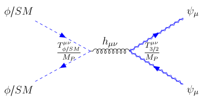
Figure 1: Feynman diagram for the production of spin-$\frac{3}{2}$ particles through the gravitational scattering of the inflaton condensate or the Standard Model particle bath.

II.1 The Rarita-Schwinger field

Naively, while looking at the table of known fundamental particles, we observe spin-0, spin-$\frac{1}{2}$, spin-1 and spin-2 fields. Naturally, one might question the absence of a spin-$\frac{3}{2}$ fundamental particle. However, it is often claimed that fields with spin higher than 1 exhibit pathologies. After the 1939 paper by Fierz and Pauli Fierz:1939ix , where they constructed the Lagrangians for spin-$\frac{3}{2}$ and spin-2 particles, Rarita and Schwinger proposed a more compact formulation for spin-$\frac{3}{2}$ particles Rarita:1941mf , leading to the equations of motion

$$(i\gamma^{\mu}\partial_{\mu}-m_{3/2})\psi_{\mu}=0\,,~{}~{}~{}\gamma^{\mu}\psi_{\mu}=0\,.$$ (1)

These equations can be obtained from the Lagrangian

$${\cal L}_{3/2}\;=\;\bar{\psi}_{\mu}(i\gamma^{\mu\rho\nu}\partial_{\rho}+m_{3/2}\gamma^{\mu\nu})\psi_{\nu}\,,$$ (2)

with

$$\gamma^{\mu\nu}\;=\;\frac{1}{2}\left[\gamma^{\mu},\gamma^{\nu}\right]=\gamma^{\mu}\gamma^{\nu}-\eta^{\mu\nu}\,,$$ (3)

and

$$\gamma^{\mu\nu\rho}\;=\;\gamma^{\mu}\gamma^{\nu}\gamma^{\rho}-\eta^{\mu\rho}\gamma^{\nu}-\eta^{\nu\rho}\gamma^{\mu}+\eta^{\mu\nu}\gamma^{\rho}\,.$$ (4)

A stable $\psi_{\mu}$ is called a raritron and can constitute the majority of the dark matter component of the Universe.

II.2 Gravitational Couplings

To compute the gravitational interactions between the raritron and the graviton, the space-time metric is expanded around Minkowski spacetime using $g_{\mu\nu}\simeq\eta_{\mu\nu}+\frac{2h_{\mu\nu}}{M_{P}}$. The Lagrangian can then be written as (see e.g., cmov ; cmosv ; hol )

$$\sqrt{-g}{\cal L}_{\rm int}\;=\;-\frac{1}{M_{P}}h_{\mu\nu}\left(T^{\mu\nu}_{\rm SM}+T^{\mu\nu}_{\phi}+T^{\mu\nu}_{\psi_{\mu}}\right)\,,$$ (5)

where SM represents Standard Model fields and $\phi$ is the inflaton. The form of the canonical stress-energy tensor $T^{\mu\nu}_{i}$ depends on the spin of the field, with $i=0,\,1/2,\,1,\,3/2$. For the inflaton and SM fields, we take

$$T^{\mu\nu}_{0} = \partial^{\mu}S\partial^{\nu}S-g^{\mu\nu}\left[\frac{1}{2}\partial^{\alpha}S\partial_{\alpha}S-V(S)\right]\,,$$ (6)

$$T^{\mu\nu}_{1/2} = \frac{i}{4}\left[\bar{\chi}\gamma^{\mu}\overset{\leftrightarrow}{\partial^{\nu}}\chi+\bar{\chi}\gamma^{\nu}\overset{\leftrightarrow}{\partial^{\mu}}\chi\right]$$ (7)

$$-g^{\mu\nu}\left[\frac{i}{2}\bar{\chi}\gamma^{\alpha}\overset{\leftrightarrow}{\partial_{\alpha}}\chi-m_{\chi}\bar{\chi}\chi\right]\,,$$

$$T_{1}^{\mu\nu} = \frac{1}{2}\left[F^{\mu}_{\alpha}F^{\nu\alpha}+F^{\nu}_{\alpha}F^{\mu\alpha}-\frac{1}{2}g^{\mu\nu}F^{\alpha\beta}F_{\alpha\beta}\right]\,,$$ (8)

where $V(S)$ is the scalar potential for either the inflaton or the SM Higgs boson, with $S=\phi,H$, and $A\overset{\leftrightarrow}{\partial}_{\mu}B\equiv A\partial_{\mu}B-(\partial_{\mu}A)B$. Here $F_{\mu\nu}=\partial_{\mu}A_{\nu}-\partial_{\nu}A_{\mu}$ is the field strength for a vector field, $A_{\mu}$. The energy-momentum tensor for a spin-$\frac{3}{2}$ Majorana field is given by tmn

$$T_{3/2}^{\mu\nu} =-\frac{i}{4}\overline{\psi}_{\rho}\gamma^{(\mu}\overset{\leftrightarrow}{\partial}{}^{\nu)}\psi^{\rho}$$ (9)

$$+\frac{i}{2}\overline{\psi}{}^{(\nu}\gamma^{\mu)}\overset{\leftrightarrow}{\partial}_{\rho}\psi^{\rho}+\frac{i}{2}\overline{\psi}^{\rho}\gamma^{(\mu}\overset{\leftrightarrow}{\partial}_{\rho}\psi^{\nu)}\,,$$

where parentheses surrounding indices indicate symmetrization, defined by $A^{(\mu}B^{\nu)}\equiv(A^{\mu}B^{\nu}+A^{\nu}B^{\mu})/2$. For a Dirac spin-3/2 field instead, the right-hand side of Eq. (9) should be multiplied by a factor of 2.

The gravitational scattering amplitudes related to the production rate of the processes

$$\phi/{\rm{SM}}^{i}(p_{1})+\phi/{\rm{SM}}^{i}(p_{2})\rightarrow\psi(p_{3})+\psi(p_{4})$$ (10)

can be parametrized by

$$\mathcal{M}^{i\frac{3}{2}}\propto M_{\mu\nu}^{\frac{3}{2}}\Pi^{\mu\nu\rho\sigma}M_{\rho\sigma}^{i}\;,$$ (11)

where $i=0,1/2,1$ denotes the spin of the initial state involved in the scattering process. Note that we are summing over all polarizations, justifying the absence of Lorentz indices in Eq. (10) for the raritron. Here, $\Pi^{\mu\nu\rho\sigma}$ is the graviton propagator for the canonical field $h_{\mu\nu}$ with momentum $k=p_{1}+p_{2}$,

$$\Pi^{\mu\nu\rho\sigma}(k)=\frac{\eta^{\mu\rho}\eta^{\nu\sigma}+\eta^{\mu\sigma}\eta^{\nu\rho}-\eta^{\mu\nu}\eta^{\rho\sigma}}{2k^{2}}\,.$$ (12)

The partial amplitudes, $M_{\mu\nu}^{i}$, can be expressed by cmov

$$M_{\mu\nu}^{0} = \frac{1}{2}\left[p_{1\mu}p_{2\nu}+p_{1\nu}p_{2\mu}-\eta_{\mu\nu}p_{1}\cdot p_{2}-\eta_{\mu\nu}V^{\prime\prime}(S)\right]\,,$$ (13)

$$M_{\mu\nu}^{\frac{1}{2}} = \frac{1}{4}{\bar{v}}(p_{2})\left[\gamma_{\mu}(p_{1}-p_{2})_{\nu}+\gamma_{\nu}(p_{1}-p_{2})_{\mu}\right]u(p_{1})\,,$$ (14)

$$M_{\mu\nu}^{1} = \frac{1}{2}\bigg{[}\epsilon_{2}^{*}\cdot\epsilon_{1}\left(p_{1\mu}p_{2\nu}+p_{1\nu}p_{2\mu}\right)$$ (15)

$$- \epsilon_{2}^{*}\cdot p_{1}\left(p_{2\mu}\epsilon_{1\nu}+\epsilon_{1\mu}p_{2\nu}\right)-\epsilon_{1}\cdot p_{2}\left(p_{1\nu}\epsilon_{2\mu}^{*}+p_{1\mu}\epsilon_{2\nu}^{*}\right)$$

$$+ p_{1}\cdot p_{2}\left(\epsilon_{1\mu}\epsilon_{2\nu}^{*}+\epsilon_{1\nu}\epsilon_{2\mu}^{*}\right)$$

$$+ \eta_{\mu\nu}\left(\epsilon_{2}^{*}\cdot p_{1}\epsilon_{1}\cdot p_{2}-p_{1}\cdot p_{2}\,\epsilon_{2}^{*}\cdot\epsilon_{1}\right)\bigg{]}\,,$$

where the masses of the SM fermions and vector fields have been neglected. The partial amplitude for the Majorana spin-$\frac{3}{2}$ field $\psi_{\mu}$ is given by

$$M_{\mu\nu}^{\frac{3}{2}} = \frac{1}{4}\left[{\bar{v}}^{\alpha}(p_{4})\gamma_{(\mu}(p_{3}-p_{4})_{\nu)}u_{\alpha}(p_{3})\right.$$ (16)

$$- 2\left.{\bar{v}}^{\alpha}(p_{4})\gamma_{(\mu}(p_{3}-p_{4})_{\alpha}u_{\nu)}(p_{3})\right.$$

$$- 2\left.{\bar{v}}_{(\nu}(p_{4})\gamma_{\mu)}(p_{3}-p_{4})_{\alpha}u^{\alpha}(p_{3})\right]\,,$$

where we defined $\psi_{\mu}(p)=u_{\mu}(p)e^{-ipx}$. In this section, we do not rely on any specific model of inflation and keep our discussion as general as possible. Any model satisfying the constraints on the slow-roll parameters as imposed by Planck data Planck will suffice, provided there is a well-defined minimum and the potential can be expanded as $V(\phi)\simeq\lambda\phi^{k}/M_{P}^{k-4}$ around this minimum. For example, both the Starobinsky model Staro and $\alpha$-attractor type models Kallosh:2013hoa are sufficient.

We consider two distinct processes illustrated by the Feynman diagram in Fig. 1:

i) The production of raritrons from the inflaton $\phi+\phi\rightarrow\psi+\psi$. In the case of a quadratic potential, the inflaton behaves like a massive particle at rest, with four-momentum $p_{1,2}$. Its partial amplitude is then directly given by Eq. (13). However, for a generic potential $V(\phi)$, we need to use the zero mode of the inflaton condensate that is valid for any arbitrary minimum (see below and cmosv for a detailed discussion).

ii) The production from the thermal background, $\textrm{SM}+\textrm{SM}\rightarrow\psi+\psi$, which uses Eqs. (6-8) for SM particles on the right-hand side of Eq. (11). In the following subsection, we compute the full scattering amplitudes for both channels and determine the gravitational production rate of the raritron.

II.3 Gravitational Production from the Inflaton Condensate

We begin by examining the gravitational production of the raritron from the inflaton condensate. Although particle production occurs throughout the reheating process, the dominant source of energy density emerges at the onset of oscillations after inflation, when the oscillation amplitude peaks. Notably, despite gravitational production process being Planck-suppressed, the inflaton condensate scattering continues to be a substantial source of particle production, particularly at the beginning of the reheating process, when its energy density is very large.

II.3.1 Quadratic potential minimum

We consider the case with a quadratic minimum first, with $V(\phi)\simeq\frac{1}{2}m_{\phi}^{2}\phi^{2}$. In this case, the rate computation is straightforward. We evaluate the square of the matrix element in Eq. (11) using $M^{0}_{\rho\sigma}$ for the inflaton incoming state. We assume for the inflaton condensate that the incoming inflaton momentum vanishes, $p_{1,2}=0$, and compute $|\mathcal{M}^{0\frac{3}{2}}|^{2}$ using the spinor sums Haberzettl:1998rw ; Ding:2012sm

$$P_{ab} \;=\;\sum_{s=-3/2}^{+3/2}u_{a}(\mathbf{p},s)\bar{u}_{b}(\mathbf{p},s)\;=\;\left(\not{p}+m_{3/2}\right)\times~{}$$

$$\left(\eta_{ab}-\frac{1}{3}\gamma_{a}\gamma_{b}-\frac{2}{3}\frac{p_{a}p_{b}}{m_{3/2}^{2}}+\frac{p_{a}\gamma_{b}-p_{b}\gamma_{a}}{3m_{3/2}}\right)\,,$$ (17)

and

$$Q_{ab} \;=\;\sum_{s=-3/2}^{+3/2}v_{a}(\mathbf{p},s)\bar{v}_{b}(\mathbf{p},s)\;=\;\left(\not{p}-m_{3/2}\right)\times~{}$$

$$\left(\eta_{ab}-\frac{1}{3}\gamma_{a}\gamma_{b}-\frac{2}{3}\frac{p_{a}p_{b}}{m_{3/2}^{2}}-\frac{p_{a}\gamma_{b}-p_{b}\gamma_{a}}{3m_{3/2}}\right)\,.$$ (18)

Using the above expressions, we find that the total matrix element squared is given by Eq. (106) shown in Appendix B. For the inflaton condensate, this expression can be simplified significantly by writing $t=m_{3/2}^{2}-m_{\phi}^{2}$ and $s=4m_{\phi}^{2}$, and the matrix element squared (106) becomes

$$|\overline{\mathcal{M}}|^{2}\;=\;\frac{m_{\phi}^{4}s}{18M_{P}^{4}m_{3/2}^{2}}\left(1-\frac{4m_{3/2}^{2}}{s}\right)\left(1-\frac{6m_{3/2}^{2}}{s}+\frac{18m_{3/2}^{4}}{s^{2}}\right)$$

$$=\frac{2}{9}\frac{m_{\phi}^{6}}{m_{3/2}^{2}M_{P}^{4}}\left(1-\frac{m_{3/2}^{2}}{m_{\phi}^{2}}\right)\left(1-\frac{3}{2}\frac{m_{3/2}^{2}}{m_{\phi}^{2}}+\frac{9}{8}\frac{m_{3/2}^{4}}{m_{\phi}^{4}}\right)\,.$$ (19)

The production rate, $R^{\phi^{k}}$, for a quadratic minimum with $k=2$, can be written as mybook

$$R^{\phi^{2}}\;=\;n_{\phi}^{2}\langle\sigma v\rangle=\frac{\rho_{\phi}^{2}}{m_{\phi}^{2}}\frac{|{\cal M}|^{2}}{32\pi m_{\phi}^{2}}\frac{p_{3}}{m_{\phi}}\,,$$ (20)

where $p_{3}=\sqrt{m_{\phi}^{2}-m_{3/2}^{2}}$, and if we use the matrix element squared (II.3.1), we find

$$R^{\phi^{2}}\;=\frac{2\times\rho_{\phi}^{2}}{288\pi M_{P}^{4}}\left(\tau^{-1}-\frac{3}{2}+\frac{9}{8}\tau\right)\left(1-\tau\right)^{3/2}\,,$$ (21)

with $\tau=m_{3/2}^{2}/m_{\phi}^{2}$. The factor of 2 explicitly accounts for the fact that 2 raritrons are produced by annihilation.

Before extending our result to a more general potential $V(\phi)$, we would like to make a few comments regarding Eq. (21). The massive raritron could have been considered, naively, as a Clebsch-Gordan decomposition of a massive spin-1 boson and a spin-$\frac{1}{2}$ fermion, which is manifestly not the case when we look at the limit $\tau\rightarrow 0$ of Eq. (21). Indeed, we would expect no production of massless fermions, due to helicity conservation MO , and no divergences are expected for the production of a massless vector field Barman:2021ugy . This reflects the inherent pathology of theories with spin $>1$, implying that we should treat with care the unitarity constraints when we analyze the bounds on $m_{3/2}$.

II.3.2 General potentials

Gravitational particle production from the inflaton condensate naturally depends on the shape of the potential. We extend our discussion and consider a more general potential which about its minimum is of the form

$$V(\phi)\;=\;\lambda\frac{\phi^{k}}{M_{P}^{k-4}}\,,\qquad\phi\ll M_{P}\,.$$ (22)

We parameterize the time-dependent oscillating inflaton field as

$$\phi(t)\;=\;\phi_{0}(t)\cdot\mathcal{P}(t)\,,$$ (23)

where $\phi_{0}(t)$ is the time-dependent envelope that includes the effects of redshift and $\mathcal{P}(t)$ describes the periodicity of the oscillation. Then for a potential of the form (22), we can write $V(\phi)=V(\phi_{0})\cdot\mathcal{P}(t)^{k}$ and expand the potential energy in terms of its Fourier modes Ichikawa:2008ne ; Kainulainen:2016vzv ; GKMO2

$$V(\phi)=V(\phi_{0})\sum_{n=-\infty}^{\infty}{\cal P}_{k,n}e^{-in\omega t}=\langle\rho_{\phi}\rangle\sum_{n=-\infty}^{\infty}{\cal P}_{k,n}e^{-in\omega t}\,,$$ (24)

where $\omega$ is the frequency of oscillation of $\phi$, given by GKMO2

$$\omega=m_{\phi}\sqrt{\frac{\pi k}{2(k-1)}}\frac{\Gamma(\frac{1}{2}+\frac{1}{k})}{\Gamma(\frac{1}{k})}\,,$$ (25)

with $m_{\phi}^{2}=\partial^{2}V/\partial\phi^{2}|_{\phi_{0}}$,

$$\mathcal{P}(t)^{k}\;=\;\sum_{n=-\infty}^{\infty}\mathcal{P}_{k,n}e^{-in\omega t}\,,$$ (26)

and $\langle\rho_{\phi}\rangle$ is the mean energy density averaged over the oscillations.

To compute the inflaton condensate scattering rate, we follow the treatment presented in Appendix C. We find that the raritron production rate is given by

$$R^{\phi^{k}}\;=\;\frac{2\times\rho_{\phi}^{2}}{72\pi M_{P}^{4}}\Sigma_{3/2}^{k}\,,$$ (27)

where

$$\Sigma_{3/2}^{k}\;=\;\sum_{n=1}^{+\infty}|\mathcal{P}_{k,n}|^{2}\frac{E_{n}^{2}}{m_{3/2}^{2}}\left(1-6\frac{m_{3/2}^{2}}{E_{n}^{2}}+18\frac{m_{3/2}^{4}}{E_{n}^{4}}\right)\times~{}$$

$$\times\left[1-\frac{4m_{3/2}^{2}}{E_{n}^{2}}\right]^{3/2}\,.$$ (28)

Here the superscript $k$ corresponds to the type of potential minimum $V(\phi)\sim\phi^{k}\sim\mathcal{P}^{k}$, $E_{n}=n\omega$ is the energy of the $n$-th mode of the inflaton oscillation, and $m_{3/2}$ is the produced raritron mass. In the quadratic case, where $\omega=m_{\phi}$ (see Eq. (25)) and ${\cal P}(t)^{2}=\cos^{2}(m_{\phi}t)=\frac{1}{2}+\frac{1}{4}(e^{-2m_{\phi}t}+e^{2m_{\phi}t})$, since $\sum|\mathcal{P}_{2,n}|^{2}=|{\cal P}_{2,2}|^{2}=\frac{1}{16}$, only the second mode in the Fourier expansion contributes to the sum. Taking $E_{2}=2m_{\phi}$, we find that the rate (27) reduces to Eq. (20).

We also consider separately the production of the $\pm\frac{1}{2}$ and $\pm\frac{3}{2}$ helicity components. One can express the spin-$\frac{3}{2}$ polarization vector as a direct product of spin-1 and spin-$\frac{1}{2}$ polarization vectors. We introduce the following spin-$\frac{3}{2}$ Clebsch-Gordan decomposition for the spinor

$$u^{\mu}_{\pm 3/2}(p) = \epsilon^{\mu}_{\pm}(p)u_{\pm 1/2}(p)\,,$$ (29)

$$u^{\mu}_{\pm 1/2}(p) = \sqrt{\frac{2}{3}}\epsilon_{0}^{\mu}(p)u_{\pm 1/2}(p)~{}$$ (30)

$$+\frac{1}{\sqrt{3}}\epsilon^{\mu}_{\pm}(p)u_{\mp 1/2}(p)\,,$$

$$v^{\mu}_{\pm 3/2}(p) = \epsilon^{\mu*}_{\pm}(p)v_{\pm 1/2}(p)\,,$$ (31)

$$v^{\mu}_{\pm 1/2}(p) = \sqrt{\frac{2}{3}}\epsilon_{0}^{\mu*}(p)v_{\pm 1/2}(p)~{}$$ (32)

$$+\frac{1}{\sqrt{3}}\epsilon^{\mu*}_{\pm}(p)v_{\mp 1/2}(p)\,.$$

We find that that the raritron production rate (27) can be decomposed as

$$R^{\phi^{k}}\;=\;\frac{2\times\rho_{\phi}^{2}}{72\pi M_{P}^{4}}\left(\Sigma_{3/2,3/2}^{k}+\Sigma_{3/2,1/2}^{k}\right)\,,$$ (33)

where the transverse spin $\pm\frac{3}{2}$ contribution is given by

$$\Sigma_{3/2,3/2}^{k}\;=\;\sum_{n=1}^{+\infty}|\mathcal{P}_{k,n}|^{2}\frac{E_{n}^{2}}{m_{3/2}^{2}}\times\left(9\frac{m_{3/2}^{4}}{E_{n}^{4}}\right)\times~{}$$

$$\times\left[1-\frac{4m_{3/2}^{2}}{E_{n}^{2}}\right]^{3/2}\,,$$ (34)

and the longitudinal spin $\pm\frac{1}{2}$ contribution is

$$\Sigma_{3/2,1/2}^{k}\;=\;\sum_{n=1}^{+\infty}|\mathcal{P}_{k,n}|^{2}\frac{E_{n}^{2}}{m_{3/2}^{2}}\times\left(1-3\frac{m_{3/2}^{2}}{E_{n}^{2}}\right)^{2}\times~{}$$

$$\times\left[1-\frac{4m_{3/2}^{2}}{E_{n}^{2}}\right]^{3/2}\,.$$ (35)

We note that the sum of transverse and longitudinal components satisfy the expression (II.3.2), with $\Sigma_{3/2}^{k}=\Sigma_{3/2,3/2}^{k}+\Sigma_{3/2,1/2}^{k}$.

Returning to the pathology of the limit $m_{3/2}\rightarrow 0$ ($\tau\rightarrow 0$) discussed above, we observe that the transverse components $\pm\frac{3}{2}$ are not produced for $m_{3/2}=0$. These components correspond to a direct composition between a spin-$\frac{1}{2}$ fermion and the transverse components of a spin-1, as we can see in Eqs. (29) and (31). As these transverse components are not gravitationally produced for massless particles MO , it stands to reason that their production rate vanishes in the massless limit for a spin-$\frac{3}{2}$ particle as well. In other words, the transverse modes are expected to be highly suppressed for light raritron, relative to the longitudinal mode which is enhanced and could be considered as the goldstino in a gauged framework.

In Fig. 2, we plot separately the longitudinal and transverse components for $k=2$. We clearly see the effect we have just described: the transverse mode is always produced in negligible quantities compared with the longitudinal mode, except in the limit where the mass of the raritron is of the order of the fundamental mode $m_{3/2}\simeq m_{\phi}$. The slopes for masses $m_{3/2}\lesssim m_{\phi}$, keeping only the first Fourier mode as an approximation, gives $R_{\pm 3/2}\propto m_{3/2}^{2}$ and $R_{\pm 1/2}\propto{m_{3/2}^{-2}}$ and do not depend on $k$. The absolute value of the rates depends on the Fourier coefficients ${\cal P}_{n,k}$ which themselves become very similar for large values of $k$, hence we do not expect big differences for larger values of $k$.

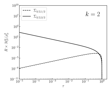
Figure 2: Longitudinal and transverse raritron production rates for $k=2$ in the units of $R\times M_{P}^{4}/\rho_{\phi}^{2}$ as a function of $\tau=m_{3/2}^{2}/m_{\phi}^{2}$. As can be seen from the figure, the raritron production is completely dominated by the longitudinal component, which contains a factor $\tau^{-1}$.

II.4 Relic abundance calculation

Given the production rate, we next compute the abundance of raritrons from the Boltzmann equation,

$$\frac{dn}{dt}+3Hn=R^{\phi^{k}}\,,$$ (36)

where $H=\frac{\dot{a}}{a}$ is the Hubble parameter. It is convenient to rewrite the Boltzmann equation in terms of the scale factor,

$$\frac{dY}{da}=\frac{a^{2}R^{\phi^{k}}}{H}\,,$$ (37)

where $Y\equiv a^{3}n$. To integrate this expression we need to include the dependence $H(a)$ with

$$H(a)=\frac{\rho^{\frac{1}{2}}_{\phi}(a)}{\sqrt{3}M_{P}}\,.$$ (38)

The conservation of energy for the inflaton field imposes

$$\frac{d\rho_{\phi}}{dt}+3(1+w)H\rho_{\phi} = Ha\left[\frac{d\rho_{\phi}}{da}+3(1+w)\frac{\rho_{\phi}}{a}\right]$$ (39)

$$= (1+w)\Gamma_{\phi}\rho_{\phi}\,,$$

whose solution is, for $\Gamma_{\phi}\ll H$

$$\rho_{\phi}(a)=\rho_{\rm end}\left(\frac{a_{\rm end}}{a}\right)^{\frac{6k}{k+2}}=\rho_{\rm RH}\left(\frac{a_{\rm RH}}{a}\right)^{\frac{6k}{k+2}}\,.$$ (40)

In these expressions, $a_{\rm end}$ is the value of the scale factor when accelerated expansion (inflation) ends, $\rho_{\rm end}=\rho_{\phi}(a_{\rm end})$, $a_{\rm RH}$ is the scale factor when $\rho_{R}(a_{\rm RH})=\rho_{\phi}(a_{\rm RH})$, defining the moment of reheating. The Boltzmann equation (37) then becomes

$$\frac{dY}{da}=\frac{\sqrt{3}M_{P}}{\sqrt{\rho_{\rm RH}}}a^{2}\left(\frac{a}{a_{\rm RH}}\right)^{\frac{3k}{k+2}}R^{\phi^{k}}(a)\,.$$ (41)

Restricting our attention to the case $k=2$, we have $\rho_{\phi}\sim a^{-3}$, $\rho_{R}\sim T^{4}\sim a^{-3/2}$, with $m_{\phi}^{2}=2\lambda M_{P}^{2}$. The Boltzmann equation becomes

$$\frac{dY}{da}=\frac{\sqrt{3}M_{P}}{\sqrt{\rho_{\rm RH}}}a^{2}\left(\frac{a}{a_{\rm RH}}\right)^{\frac{3}{2}}R^{\phi^{2}}(a)\,,$$ (42)

where $R^{\phi^{2}}(a)$ is given by Eq. (21). Eq. (42) is easily integrated to give

$$n(a_{\rm RH}) = \frac{1}{72\sqrt{3}\pi M_{P}}\left(\frac{\rho_{\rm end}}{M_{P}^{4}}\right)^{\frac{1}{2}}\alpha T_{\rm RH}^{4}$$ (43)

$$\times\left(\tau^{-1}-\frac{3}{2}+\frac{9}{8}\tau\right)\left(1-\tau\right)^{3/2}\,,$$

where we assumed that $a_{\rm RH}\gg a_{\rm end}$ and $\alpha$ is defined by

$$\rho_{R}\;=\;\frac{g_{T}\pi^{2}}{30}T^{4}\equiv\alpha T^{4}\,.$$ (44)

Using mybook

$$\Omega h^{2}\simeq 1.6\times 10^{8}\frac{g_{0}}{g_{\rm RH}}\frac{n(T_{\rm RH})}{T_{\rm RH}^{3}}\frac{m_{3/2}}{1~{}{\rm GeV}}\,,$$ (45)

we then obtain

$$\Omega h^{2} \simeq 3\times 10^{9}\left(\frac{T_{\rm RH}}{10^{10}{\rm GeV}}\right)\left(\frac{\rho_{\rm end}}{(5.2\times 10^{15}{\rm GeV})^{4}}\right)^{\frac{1}{2}}$$ (46)

$$\left(\frac{m_{\phi}}{1.7\times 10^{13}{\rm GeV}}\right)^{2}\left(\frac{{\rm EeV}}{m_{3/2}}\right)\,,$$

where we take $g_{0}=43/11$ and $g_{\rm RH}=427/4$, and assume $m_{3/2}\ll m_{\phi}$, and values of $m_{\phi}$ and $\rho_{\rm end}$ are normalized for an $\alpha$-attractor model of inflation with $k=2$, though there is some additional dependence on $T_{\rm RH}$ for these quantities GKMO1 ; cmov ; egnov .

As one can see, the gravitational production of raritrons is extremely efficient, much more efficient than the production of scalars, spin-$\frac{1}{2}$ fermions, or vectors MO . As a consequence, stable raritrons are only possible if either $T_{\rm RH}$ is quite low (of order the weak scale or below) or $m_{3/2}\simeq m_{\phi}$. This can be seen in Fig. 3 where the red curve shows the values of $m_{3/2}$ and $T_{\rm RH}$ such that $\Omega h^{2}=0.12$ from Eq. (46). To remain consistent with big bang nucleosynthesis, $T_{\rm RH}\gtrsim 2$ MeV, which implies that raritron dark matter is heavier than $\gtrsim 6$ PeV. This unavoidable (because it is produced gravitationally) minimal mass for the raritron is one of the main results of our work.

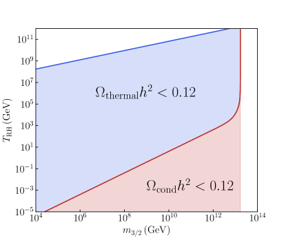
Figure 3: Contours of $\Omega_{\rm cond}h^{2}=0.12$ (red) and $\Omega_{\rm thermal}h^{2}=0.12$ (blue) in the $(m_{3/2},T_{\rm RH})$ plane.

Using Eqs. (33)-(35), it is possible to separate out the contributions of the transverse and longitudinal contributions to $\Omega_{\frac{3}{2}}$. For the transverse contribution for $k=2$ we have

$$n_{\frac{3}{2}}(a_{\rm RH})=\frac{1}{128\sqrt{3}\pi M_{P}}\left(\frac{\rho_{\rm end}}{M_{P}^{4}}\right)^{\frac{1}{2}}\alpha T_{\rm RH}^{4}\tau(1-\tau)^{\frac{3}{2}}\,,$$ (47)

and

$$\Omega_{\frac{3}{2}}h^{2} \simeq 2\times 10^{-8}\left(\frac{T_{\rm RH}}{10^{10}~{}{\rm GeV}}\right)\left(\frac{\rho_{\rm end}}{(5.2\times 10^{15}{\rm GeV})^{4}}\right)^{\frac{1}{2}}$$ (48)

$$\left(\frac{1.7\times 10^{13}{\rm GeV}}{m_{\phi}}\right)^{2}\left(\frac{m_{3/2}}{{\rm EeV}}\right)^{3}\,.$$

As expected and discussed previously, the gravitational production of the transverse mode is completely negligible.

Similarly, we can compute the longitudinal contribution

$$n_{\frac{1}{2}}(a_{\rm RH}) = \frac{1}{72\pi\sqrt{3}M_{P}}\left(\frac{\rho_{\rm end}}{M_{P}^{4}}\right)^{\frac{1}{2}}\alpha T_{\rm RH}^{4}$$ (49)

$$\times\left(\tau^{-1}-\frac{3}{2}+\frac{9}{16}\tau\right)\left(1-\tau\right)^{3/2}\,,$$

which for $m_{3/2}\ll m_{\phi}$, gives the result in Eq. (46) for $\Omega_{\frac{1}{2}}h^{2}$ since the production of raritrons is completely dominated by the longitudinal component which carries the factor of $\tau^{-1}$.

At this point it is important to note that for “low” values of $\tau$, we may run into a problem with unitarity. The amplitude in Eq. (II.3.1) becomes of order unity when $m_{3/2}\lesssim 1$ TeV. However, raritron scattering $\psi_{\mu}\psi_{\mu}\to h_{\mu\nu}\to\psi_{\mu}\psi_{\mu}$ is further enhanced, and we estimate that its amplitude scales as $|\mathcal{M}|^{2}\propto m_{\phi}^{4}/(M_{P}^{4}\tau^{4})$, which would exceed unity when $m_{3/2}\lesssim 40$ EeV! This would allow reheating temperatures $T_{\rm RH}\gtrsim 10$ GeV.

Finally, we can also generalize this result to cases when $k\neq 2$. We find that the number density can be expressed as

$$n(a_{\rm RH})\;=\;\frac{(k+2)}{(k-1)}\frac{\rho_{\rm RH}^{3/2}}{72\sqrt{3}\pi M_{P}^{3}}\left(\frac{\rho_{\rm end}}{\rho_{\rm RH}}\right)^{1-\frac{1}{k}}\Sigma_{3/2}^{k}\,,$$ (50)

and the dark matter abundance becomes

$$\Omega h^{2}\simeq 2.2\times 10^{5}\frac{(k+2)}{(k-1)}\left(\frac{\rho_{\rm end}}{\rho_{\rm RH}}\right)^{1-\frac{1}{k}}\frac{\rho_{\rm RH}^{3/4}}{M_{P}^{3}}\frac{m_{3/2}}{1~{}{\rm GeV}}\Sigma_{3/2}^{k}\,.$$ (51)

As expected, for $k=2$ this expression reduces to Eq. (46).

II.5 Gravitational Production of Raritrons from the Thermal Bath

The production of raritron dark matter from the thermal bath is also possible. The scattering of SM particles includes the Higgs scalars, gauge bosons, and fermions in the initial state. Since the initial particle momenta $p_{1}$ and $p_{2}$ are large (of order $m_{\phi}$) at the beginning of reheating and dominate over electroweak scale quantities, we assume that the initial particle states are massless.

For the Higgs initial state we can use Eq. (106) with the association $\phi\to h$ and set $m_{\phi}=0$ (i.e., we neglect the Higgs mass, and all SM masses relative to the reheating temperature in the thermal bath). In this case, Eq. (106) reduces to

$$|{\cal M}^{0}|^{2}=\frac{1}{72m_{3/2}^{4}M_{P}^{4}s^{2}}\left[-s^{2}t(s+t)(s+2t)^{2}-72m_{3/2}^{12}\right.$$ (52)

$$+24m_{3/2}^{10}(7s+12t)-2m_{3/2}^{8}\left(47s^{2}+264st+216t^{2}\right)$$

$$+m_{3/2}^{6}\left(-2s^{3}+244s^{2}t+576st^{2}+288t^{3}\right)$$

$$+m_{3/2}^{4}\left(s^{4}-34s^{3}t-210s^{2}t^{2}-240st^{3}-72t^{4}\right)$$

$$\left.+m_{3/2}^{2}s\left(s^{4}+6s^{3}t+44s^{2}t^{2}+64st^{3}+24t^{4}\right)\right]\,.$$

In addition to the production of raritrons from a Higgs initial state, other SM particles in thermal bath will also lead to raritron production. The amplitudes for massless fermion and gauge boson initial states are given in Eqs. (108) and (109) respectively.

The dark matter production rate $R(T)$ for the SM+SM $\rightarrow$ $\psi+\psi$ process with amplitude $\cal{M}$ is given by Benakli:2017whb ; grav2 ; mybook

$$R(T) = \frac{2}{1024\pi^{6}}\times\int f_{1}f_{2}E_{1}\mathop{}\!\mathrm{d}E_{1}E_{2}\mathop{}\!\mathrm{d}E_{2}\mathop{}\!\mathrm{d}\cos\theta_{12}$$ (53)

$$\times\int|\overline{\cal M}|^{2}\mathop{}\!\mathrm{d}\Omega_{13}\,,$$

where we assumed that $s\gg 4m_{3/2}^{2}$, and the factor of two accounts for two raritrons produced per scattering, $E_{i}$ denotes the energy of particle $i=1,2,3,4$. $\theta_{13}$ and $\theta_{12}$ are the angles formed by momenta ${\bf{p}}_{1,3}$ (in the center-of-mass frame) and ${\bf{p}}_{1,2}$ (in the laboratory frame), respectively. The infinitesimal solid angle in the above integral is then $\mathop{}\!\mathrm{d}\Omega_{13}=2\pi\mathop{}\!\mathrm{d}\cos\theta_{13}$. In addition,

$$f_{i}=\frac{1}{e^{E_{i}/T}\pm 1}\,,$$ (54)

represents the assumed thermal distributions of the incoming SM particles.

The total amplitude squared for the gravitational scattering process SM+SM $\rightarrow$ $\psi+\psi$ is given by a sum of the three amplitudes associated with three different SM initial state spins,

$$|\overline{\mathcal{M}}|^{2}=4|\overline{\mathcal{M}}^{0}|^{2}+45|\overline{\mathcal{M}}^{1/2}|^{2}+12|\overline{\mathcal{M}}^{1}|^{2}\,.$$ (55)

Using this amplitude and performing the thermal integration in Eq. (53), we find that the raritron production rate can be parameterized by

$$R^{T}_{\frac{3}{2}}= R_{\frac{3}{2}}(T)=\beta_{1}\frac{T^{12}}{m_{3/2}^{4}M_{P}^{4}}+\beta_{2}\frac{T^{10}}{m_{3/2}^{2}M_{P}^{4}}$$ (56)

$$+\beta_{3}\frac{T^{8}}{M_{P}^{4}}+\beta_{4}\frac{m_{3/2}^{2}T^{6}}{M_{P}^{4}}+\beta_{5}\frac{m_{3/2}^{4}T^{4}}{M_{P}^{4}}\,,$$

where the numerical coefficients together with the details of the computation are given in Appendix B.

The gravitational scattering within the thermal plasma produces the raritrons. We focus on the case $k=2$ and show that the thermal production rate is strongly sub-dominant compared to the production from the inflaton condensate. Following the same steps as in the previous subsection, we replace the rate in Eq. (41) by the thermal raritron production rate (56). After expressing the temperature as function of the scale factor by solving

$$\frac{d\rho_{R}}{da}+4\frac{\rho_{R}}{a}=\frac{\Gamma_{\phi}\rho_{\phi}}{Ha}\,,$$ (57)

we find that the thermally-produced number density is given by

$$n^{T}(T_{\rm RH})=\frac{2\beta_{1}}{\alpha^{3}}\frac{\sqrt{3}\rho_{\rm RH}^{5/2}}{m_{3/2}^{4}M_{P}^{3}}\ln\left(\frac{\sqrt{\rho_{\rm end}}}{\sqrt{\alpha}T_{\rm RH}^{2}}\right)~{}$$

$$+\frac{4\beta_{2}}{\sqrt{3}\alpha^{5/2}}\frac{\rho_{\rm RH}^{2}}{m_{3/2}^{2}M_{P}^{3}}+\frac{2\beta_{3}}{\sqrt{3}}\frac{\rho_{\rm RH}^{3/2}}{M_{P}^{3}}~{}$$

$$+\frac{4\beta_{4}}{3\sqrt{3}\alpha^{3/2}}\frac{\rho_{\rm RH}m_{3/2}^{2}}{M_{P}^{3}}+\frac{\beta_{5}}{\sqrt{3}\alpha}\frac{\sqrt{\rho_{\rm RH}}m_{3/2}^{4}}{M_{P}^{3}}\,.$$ (58)

We note that in our computation, we assumed that $4m_{3/2}^{2}\ll s$, where $s=(p_{1}+p_{2})^{2}$, which would approximately correspond to $m_{3/2}\lesssim T_{\rm RH}$, and we integrated Eq. (41) between $a_{\rm end}$ and $a_{\rm RH}$. Moreover, since $\beta_{1}\simeq 3.6$ is greater than $\beta_{i=2...5}$, the first term dominates the production process for $m_{\frac{3}{2}}<T_{\rm RH}$.

Using Eq. (45) for the the relic abundance, we obtain

$$\Omega^{T}h^{2} = 5.9\times 10^{6}\,\frac{n^{T}(T_{\rm RH})}{T_{\rm RH}^{3}}\frac{m_{3/2}}{1~{}{\rm GeV}}$$ (59)

$$\simeq 3.6\times 10^{-5}\left(\frac{T_{\rm RH}}{10^{10}~{}{\rm GeV}}\right)^{7}\left(12+\ln\left(\frac{10^{10}{\rm GeV}}{T_{\rm RH}}\right)\right)$$

$$\times\left(\frac{{\rm EeV}}{m_{3/2}}\right)^{3}\,,$$

where, in the approximation, we considered only the first term in Eq. (58). In Fig. 3, we show in blue the constraint on the relic abundance in the $(m_{3/2},T_{\rm RH})$ plane from raritrons produced gravitationally from the thermal plasma. As expected, the relic density generated by the thermal source is negligible compared with that generated by inflaton oscillations in all of the parameter space. This result is also valid for $k>2$.

III Gravitino dark matter

The cosmological production of gravitinos has been a constant source of potential cosmological problems due to its over-production. Standard thermal production (discussed briefly in Section III.4 below) sets upper limits to the reheating temperature after inflation nos ; ehnos ; kl ; ekn ; bbb ; riotto ; egnop ; GMOP . There is also a non-thermal contribution to gravitino production when supersymmetry is broken during inflation riotto ; Kallosh:1999jj ; Giudice:1999yt ; Kallosh:2000ve ; Nilles:2001ry ; Nilles:2001fg ; Ema:2016oxl . In these cases, as we will see as well below, it is the goldstino which is produced (i.e., the longitudinal component, rather than the transverse component), and this is typically the inflatino (the superpartner of the inflaton) during and immediately after inflation. Indeed it was argued that the longitudinal component of the gravitino at low energy may be unrelated to the inflatino produced after inflation Nilles:2001ry ; Nilles:2001fg . Whether or not the production of inflatinos is problematic is a model dependent question and inflatino production may even be kinematically suppressed Nilles:2001my . Non-thermal production may also occur if the gravitino sound speed vanishes Benakli:2014bpa ; hase ; Kolb:2021xfn . However in this case, unless the models are constrained by eliminating the pseudoscalar, fermionic, and auxiliary components of the inflaton, no catastrophic production occurs Dudas:2021njv ; Terada:2021rtp ; Antoniadis:2021jtg .

In the remainder of this section, we consider first toy models involving two Majorana fermions coupled to the inflaton. This is a (highly) simplified example of the inflaton coupling to the gravitino and inflatino. In this case, as in the non-thermal production of the raritron, the longitudinal component of the gravitino may be easily overproduced. However, as we just alluded, the produced state may not be the longitudinal component of the gravitino at low energy. Finally, we consider a specific model of inflation and supersymmetry breaking. If reheating is prolonged, the gravitino may be produced though with a suppressed abundance.

III.1 Toy models

In the previous section, we considered the gravitational production of raritrons from the inflaton condensate and thermal bath. As we have seen in Fig. 3, the production from the condensate is dominant, and from Fig. 2, we see that the production of the longitudinal (spin-$\frac{1}{2}$) component dominates over the transverse (spin-$\frac{3}{2}$) component, particularly at low masses. In addition, as we will be interested in the production of gravitinos from the inflaton condensate as a concrete example in the next subsection, we would like to consider a toy model (not based on supergravity) which couples two spin-$\frac{1}{2}$ Majorana fields, $\psi$ and $\chi$, to the inflaton. We will consider the production of $\psi$ through $\chi$–exchange having in mind the production of a goldstino through inflatino exchange when considering the supersymmetric analogue.

The toy model assumes a Yukawa coupling of the form

$${\cal L}_{\rm int}\;=\;-y\phi\bar{\chi}\psi+h.c.\,,$$ (60)

and a direct coupling of the inflaton to a pair of $\psi$’s is absent. We further assume $m_{\chi}>m_{\phi}>m_{\psi}$ in our setup, so a direct decay of $\phi\to\chi\psi$ is not allowed kinematically. The coherent oscillation of $\phi$ during reheating can however still produce $\psi$ through $\phi\phi\to\psi\psi$ by exchanging $\chi$, whose diagrams are shown in Fig. 4.

Figure 4: Feynman diagrams of the dark matter production processes.

As in the case of raritron production in the previous section, the abundance of $\psi$ can be obtained by integrating the Boltzmann equation given the production rate $\Gamma_{\phi\phi\to\psi\psi}\rho_{\phi}/m_{\phi}$

$$R(t) = \frac{2\times y^{4}}{\pi}\frac{\rho_{\phi}^{2}}{m_{\phi}^{4}}\frac{\tau_{\psi}(1-\tau_{\psi})^{3/2}}{(1+\tau_{\chi}-\tau_{\psi})^{2}}\,,$$ (61)

where $\tau_{i}\equiv m_{i}^{2}/m_{\phi}^{2}$. As for previous rates, the factor of 2 in the numerator explicitly accounts for the fact that two $\psi$’s are produced per reaction. Using this rate, the Boltzmann equation (41) can be integrated to give

$$n(a_{\rm RH}) = \frac{4y^{4}M_{P}^{3}}{\sqrt{3}\pi m_{\phi}^{4}}\left(\frac{\rho_{\rm end}}{M_{P}^{4}}\right)^{\frac{1}{2}}\alpha T_{\rm RH}^{4}$$ (62)

$$\times\frac{\tau_{\psi}(1-\tau_{\psi})^{3/2}}{(1+\tau_{\chi}-\tau_{\psi})^{2}}\,,$$

and

$$\Omega_{\psi}h^{2} \simeq 0.12y^{4}\left(\frac{T_{\rm RH}}{10^{10}~{}{\rm GeV}}\right)\left(\frac{1.7\times 10^{13}~{}{\rm GeV}}{m_{\phi}}\right)^{2}\left(\frac{\rho_{\rm end}}{(5.2\times 10^{15}{\rm GeV})^{4}}\right)^{\frac{1}{2}}\left(\frac{10^{14}~{}{\rm GeV}}{m_{\chi}}\right)^{4}\left(\frac{m_{\psi}}{33~{}{\rm TeV}}\right)^{3}\,,$$ (63)

where we have taken the limit that $m_{\chi}\gg m_{\phi}\gg m_{\psi}$. Given the above normalizations, the spin-$\frac{1}{2}$ fermion will provide the correct relic density when $m_{\psi}\simeq 33$ TeV. One further sees that rather than a divergence at small $m_{\psi}$, the relic density goes to 0, in this limit. This can be easily understood on the basis of helicity conservation. Fig. 5 shows the parameter space satisfying $\Omega_{\psi}h^{2}=0.12$ with $y=1$, $m_{\phi}=1.7\times 10^{13}$ GeV, and $\rho_{\rm end}=(5.2\times 10^{15}~{}{\rm GeV})^{4}$. Indeed, because of the helicity suppression, the relic density of $\psi$ scales as $m_{\psi}^{3}$ as opposed to $m_{3/2}^{-1}$ and hence we see very different behaviors when comparing the results in Fig. 3 and Fig. 5.

Figure 5: The $(m_{\psi},T_{\rm RH})$ plane showing lines for $\Omega_{\psi}h^{2}=0.12$ with $m_{\chi}/m_{\phi}=1$ and 10 as labeled as well as $y=1$, $m_{\phi}=1.7\times 10^{13}$ GeV, and $\rho_{\rm end}=(5.2\times 10^{15}~{}{\rm GeV})^{4}$. The red lines correspond to the relic density obtained from Eq. (63) which was derived from the Lagrangian in Eq. (60) (without the assumption $\tau_{\chi}\gg 1$). The blue lines show the analogous result derived from the Lagrangian (64).

We can also consider a similar toy model which matches more closely the supergravity couplings of the gravitino longitudinal mode. This simple Lagrangian can be written as

$${\cal L}_{\rm int}\;=\;-\frac{y}{M_{P}}\partial_{\mu}\phi\bar{\chi}\gamma^{\mu}\psi+h.c.\,.$$ (64)

Repeating the above exercise to calculate the production rate of $\psi$, we find

$$R(t) = \frac{2\times y^{4}}{\pi}\frac{\rho_{\phi}^{2}}{M_{P}^{4}}\frac{\tau_{\psi}(1-\tau_{\psi})^{3/2}}{(1+\tau_{\chi}-\tau_{\psi})^{2}}\,,$$ (65)

which is suppressed relative to the rate in Eq. (61) by a factor of $(m_{\phi}/M_{P})^{4}$. The integration of the rate will be identical and the number density of $\psi$’s in Eq. (62) will be suppressed by the same factor. As a result, the mass needed to achieve $\Omega_{\psi}h^{2}=0.12$ is significantly larger, $m_{\psi}\simeq 2.4\times 10^{11}$ GeV. The relation between $T_{\rm RH}$ and $m_{\psi}$ is also shown in Fig. 5. As one can clearly see, the derivative coupling leading to the suppression requires a significantly larger mass, $m_{\psi}$ for a given reheating temperature in order to achieve the same relic density.

III.2 Inflatino exchange

We next turn to the example of the gravitino in supergravity models. When supergravity models of inflation are considered, gravitino ($\psi_{\mu}$) generally couples to the inflaton ($\Phi$) and the inflatino ($\chi$) through the following terms:

$${\cal L}_{\rm int} = -\frac{i}{\sqrt{2}M_{P}}\left[(\partial_{\mu}\Phi)^{*}\bar{\psi}_{\nu}\gamma^{\mu}\gamma^{\nu}P_{L}\chi-(\partial_{\mu}\Phi)\bar{\chi}P_{R}\gamma^{\nu}\gamma^{\mu}\psi_{\nu}\right].$$

In the following argument, we assume that the imaginary part of $\Phi$ is strongly stabilized, and the canonically-normalized real part $\phi\equiv\sqrt{2}{\rm Re}\Phi$ is oscillating with an inflaton potential $V(\phi)$ after the end of inflation.

In addition to the gravitational production of gravitinos discussed previously, a pair of gravitinos can also be produced from inflaton condensate via inflatino exchange. There are both the t- and u-channels shown in Fig. 4 with the replacement of $\psi\to\psi_{\mu}$. Here, we are making the (naive) assumption, that the supersymmetry breaking sector is distinct from the inflationary sector and that the inflaton does not break supersymmetry. In this case, the goldstino (or spin-$\frac{1}{2}$ component of the gravitino) is distinct from the inflatino. We return to a more realistic example in the next section. In the Boltzmann equation, the production rate $R(t)$ is computed as

$$R(t) = \frac{2\rho_{\phi}^{2}}{9\pi M_{P}^{4}}\frac{(1-\tau_{3/2})^{7/2}}{\tau_{3/2}(1+\tau_{\chi}-\tau_{3/2})^{2}}\,,$$ (67)

where we have assumed $k=2$. Note that as discussed in Appendix C, only the spin-$\frac{1}{2}$ component of $\psi_{\mu}$ is produced. Details of the computation of the production rate are also given in Appendix C. It is also interesting to see, by comparing equations (61) and (67), that the production of the longitudinal component of $\psi_{\mu}$ (the spin-$\frac{1}{2}$ part) is enhanced $\propto m_{3/2}^{-4}$ for light gravitino compared to the production of a spin-$\frac{1}{2}$ fermion (61) for reasons similar to those invoked when discussing the gravitational production of the raritrons.

With this rate, the number density of gravitinos is obtained by solving Eq. (41),

$$n(a_{\rm RH}) = \frac{4}{9\sqrt{3}\pi M_{P}}\left(\frac{\rho_{\rm end}}{M_{P}^{4}}\right)^{\frac{1}{2}}\alpha T_{\rm RH}^{4}$$ (68)

$$\times\frac{(1-\tau_{3/2})^{7/2}}{\tau_{3/2}(1+\tau_{\chi}-\tau_{3/2})^{2}}\,.$$

When $\tau_{\chi}\simeq 1$, and $\tau_{3/2}\ll 1$, this number density is roughly 8 times larger than that from graviton exchange given in Eq. (43). It should not be surprising that the two results (43) and (68) are so similar, since the exchange of a graviton involves couplings of the order $\partial_{\mu}/M_{P}$ generated by terms of the type $T_{\mu\nu}/M_{P}$, which have exactly the same form as the couplings between the inflaton, the inflatino and gravitino given in Eq. (LABEL:eq:L_gravitino). Only the graviton propagator differs from the inflatino propagator, but only in its structure, not in its order of magnitude.

The relic gravitino abundance can be then estimated by using Eq. (45)

$$\Omega h^{2} \simeq 2.4\times 10^{10}\left(\frac{T_{\rm RH}}{10^{10}{\rm GeV}}\right)\left(\frac{\rho_{\rm end}}{(5.2\times 10^{15}{\rm GeV})^{4}}\right)^{\frac{1}{2}}$$ (69)

$$\left(\frac{m_{\phi}}{1.7\times 10^{13}{\rm GeV}}\right)^{2}\left(\frac{{\rm EeV}}{m_{3/2}}\right)\,,$$

which is, as expected, about 8 times larger than Eq. (46). Furthermore as we saw previously this abundance is highly dominated by the spin-$\frac{1}{2}$ component. However, as we stressed earlier, this result ignores any contribution to supersymmetry breaking from the inflaton sector and any possible mixing between the spin-$\frac{1}{2}$ partner of the inflation, the inflatino, and the partner of the scalar associated with supersymmetry breaking in the vacuum.

III.3 Specific Supergravity Model

Let us now consider a more realistic example, in which the identity of the goldstino evolves during the reheating process kmov ; Dudas:2021njv . To be more specific, we consider a model based on no-scale supergravity no-scale . The Kähler potential can be written as

$$K=-3\ln\left[\Phi+\overline{\Phi}-\frac{1}{3}(|S|^{2}+|z|^{2})+g(S,\overline{S})+h(z,\overline{z})\right]\,.$$

The inflaton, $\phi$, is the real part of the canonically-normalized field, $\Phi\simeq\frac{1}{2}e^{\sqrt{2/3}\phi}$ (up to a small correction of order $\mu^{2}$ (defined below)). The matter-like field $S$ and Polonyi field $z$ are stabilized by $g(S,\overline{S})=|S|^{4}/\Lambda_{S}^{2}$ and $h(z,\overline{z})=|z|^{4}/\Lambda_{z}^{2}$ ekn3 ; strongpol ; dlmmo ; ADinf ; ego ; dgmo ; kmov ; eno7 ; egno4 ; enov4 ; building . The inflaton can decay into gauge bosons and gauginos if the gauge kinetic function depends on the inflaton field value ekoty ; klor ; Terada:2014uia ; dlmmo ; egno4 ; building . Barring a direct superpotential coupling of the inflaton to SM fields, this is the dominant decay mechanism in low-scale supersymmetric models. In models of high-scale supersymmetry, the inflaton decays predominately into a pair of the SM Higgs bosons egno4 ; dgmo ; dgkmo ; KMO ; kmov . The choice of the inflaton sector superpotential Cecotti

$$W_{\rm inf}\;=\;\sqrt{3}m_{\phi}S(\Phi-1/2)$$ (71)

gives the Starobinsky-like inflaton potential eno7 ; FeKR ; EGNO2 , and the inflaton energy density at the end of inflation becomes $\rho_{\rm end}=0.175m_{\phi}^{2}M_{P}^{2}$ with $m_{\phi}=3\times 10^{13}$ GeV egno5 ; egnop . The inflatino is nearly degenerate in mass with inflaton. The scalar and fermionic components of $S$ are also nearly degenerate with the inflaton kmov (note that $\Lambda_{S}$ does not affect the spectrum at leading order).

One should, however, be careful about the time dependence of the mixing in the goldstino mode. The goldstino in a non-static background is given by Nilles:2001fg $\nu=G_{I}\chi^{I}+\not{\partial}\phi_{I}\chi^{j}G_{J}^{I}$, where $G\equiv K+\ln|W|^{2}$, $G_{I}\equiv\partial G/\partial\phi^{I}$, and $G_{J}^{I}\equiv\partial G/\partial\phi^{I}\partial{\phi^{*}}^{J}$ with $\phi^{I}$ a superfield that participates in super-Higgs mechanism, and $\chi^{I}$ is the fermionic component in $\phi^{I}$. We consider the Polonyi sector superpotential, given by pol

$$W_{P}\;=\;\widetilde{m}(z+b)\,,$$ (72)

with $b\simeq 1/\sqrt{3}$. When the reheating phase begins, the various contributions to the goldstino are given by

$$G_{\Phi}\simeq-\sqrt{\frac{3}{2}}\phi,~{}G_{S}\simeq 2\mu+\sqrt{\frac{3}{2}}\frac{\phi}{\mu},$$

$$G_{z}\simeq\sqrt{3}-\frac{3}{\sqrt{2}}\phi,~{}\not{\partial}\Phi G_{\Phi}^{\Phi}\simeq m_{\phi}\phi\,,$$ (73)

where $\mu\equiv\widetilde{m}/m_{\phi}\ll 1$.

Initially, when $\phi\gg\mu M_{P}$, supersymmetry is broken by the F-term of $S$. As discussed earlier, for the quadratic case considered here ($k=2$), the energy density of the inflaton scales as $\frac{1}{2}m_{\phi}^{2}\phi^{2}\propto a^{-3}$ and $\phi\propto a^{-\frac{3}{2}}$ during reheating. But when $\phi/\mu\lesssim 1$, the primary component of the goldstino becomes the fermionic partner of the Polonyi field, $z$. We can estimate the corresponding scale factor $a_{\rm p}$, when $\phi/\mu=1$ using $\phi_{\rm p}=\phi_{\rm end}(a_{\rm end}/a_{\rm p})^{3/2}$, and $\phi_{\rm end}=\sqrt{2\rho_{\rm end}}/m_{\phi}$, then

$$\frac{a_{\rm p}}{a_{e}}=\left(\frac{\sqrt{2\rho_{e}}}{M_{P}{\tilde{m}}}\right)^{\frac{2}{3}}\,,$$ (74)

and

$$\frac{a_{\rm p}}{a_{\rm RH}}=\left(\frac{2\rho_{\rm RH}}{M_{P}^{2}{\tilde{m}}^{2}}\right)^{\frac{1}{3}}\,.$$ (75)

It would be tempting to deduce that for $a>a_{\rm p}$, the Polonyi field dominates in the goldstino and is produced by the inflaton condensate. However, this ignores the mixing between the states. Furthermore, the degree of mixing Nilles:2001fg , $\Delta$, gives rise to the gravitino sound speed, $c_{s}^{2}=1-\Delta^{2}$, which can be expressed as Kolb:2021xfn

$$\Delta^{2}=\frac{4}{\left(|\dot{\varphi}|^{2}+|F|^{2}\right)^{2}}\,\left\{|\dot{\varphi}|^{2}|F|^{2}-\left|\dot{\varphi}\cdot F^{*}\right|^{2}\right\}\;,$$ (76)

where $F^{i}\equiv{\rm e}^{K/2}K^{ij^{*}}(W_{j}+K_{j}W)$, and the $D$-term is absent in our analysis. The dot operator in Eq. (76) denotes a scalar product with the Kähler metric $K_{ij}$, namely $|\dot{\varphi}|^{2}=\dot{\varphi}^{i}\,K_{ij^{*}}\,\dot{\varphi}^{j*}$, and analogously for the other terms. As noted earlier if the gravitino sound speed vanishes Benakli:2014bpa ; hase ; Kolb:2021xfn , catastrophic production of gravitinos ensues. Likewise, in the absence of mixing, divergent (as $m_{3/2}\to 0$) production of gravitinos ensues as seen in Eqs. (68) and (69). In the absence of constraints (for example the imposition of nilpotent fields), mixing is sufficiently large so as to suppress this non-thermal source of gravitino production Dudas:2021njv ; Terada:2021rtp ; Antoniadis:2021jtg . Indeed the three-field model considered here, was also considered in Dudas:2021njv . There, it was found that although the leading contribution to the sound speed may be small, the mixing parameter, $\Delta$, in this case is large. The detailed numerical analysis in a two-field model Nilles:2001fg showed that the primary consequence of the mixing is that even though supersymmetry is initially broken ($a<a_{\rm p}$) by the inflationary sector and later ($a>a_{\rm p})$ through the Polonyi sector, the eigenstates rotate and the heavy mass eigenstate associated with the inflatino is always the field which is predominantly produced. Though a full numerical analysis of the three-field model was not performed, it was concluded that due to the large mixing, there is no catastrophic production of gravitinos in this model.

It is interesting to note that the Lagrangian (LABEL:eq:L_gravitino), suitably extended to include the coupling of the Polonyi field to the gravitino, can be separated into the parts providing the couplings of the transverse and longitudinal components. The latter will contain the mixing between the “flavor” eigenstates. This Lagrangian, written in Nilles:2001fg , contains the basic elements found in our toy Lagrangian in Eq. (64). In agreement with the numerical results found in Nilles:2001fg , our calculation of the production of $\psi$ is suppressed for low $m_{\psi}$.

In the remainder of this section, we briefly review the standard thermal production of gravitinos.

III.4 Thermal production

Before concluding this section, we can compare the production mechanisms above with the well known thermal production of gravitinos bbb ; egnop ; GMOP . So long as the scale of supersymmetry breaking is below the inflationary scale, gravitinos can be singly produced, for example, by the scattering of two gluons producing a gluino and gravitino. Here, we use the parametrization in egnop ; GMOP and consider only the gauge boson contribution to the production cross section, which we approximate as

$$\langle\sigma v\rangle\simeq\frac{26.24}{M_{P}^{2}}\left(1+0.56\,\frac{m_{1/2}^{2}}{m_{3/2}^{2}}\right)\,.$$ (77)

For $m_{3/2}$ significantly less than an assumed universal (at the GUT scale) gaugino mass, $m_{1/2}$, the 2nd term corresponding to the production of the longitudinal mode dominates. The production rate can then be written as

$$R_{1}\simeq 0.4\frac{T^{6}}{M_{P}^{2}}\left(1+0.56\,\frac{m_{1/2}^{2}}{m_{3/2}^{2}}\right)\,.$$ (78)

Integrating this rate (for $k=2$) we arrive at

$$n(a_{\rm RH})=\frac{4\sqrt{3}}{9\sqrt{\alpha}}\frac{0.4}{M_{P}}T_{\rm RH}^{4}\left(1+0.56\,\frac{m_{1/2}^{2}}{m_{3/2}^{2}}\right)\,,$$ (79)

and

$$\Omega h^{2}\simeq 0.04\left(\frac{T_{\rm RH}}{10^{10}{\rm GeV}}\right)\left(\frac{m_{3/2}}{100~{}{\rm GeV}}\right)\left(1+0.56\,\frac{m_{1/2}^{2}}{m_{3/2}^{2}}\right)\,,$$ (80)

which gives the typical upper limit on the reheating temperature in supersymmetric models of $T_{\rm RH}\lesssim 2\times 10^{10}$ GeV, for $m_{1/2}\simeq m_{3/2}=100$ GeV, and the limit becomes stronger when $m_{1/2}>m_{3/2}$. This limit results from the fact that the gravitino mass is related to the gaugino mass in a specific framework of SUSY breaking. We have neglected a kinematic factor which roughly requires $T_{\rm RH}\gtrsim m_{3/2}$. Note that for these models we are using $g_{\rm RH}=915/4$.

In the case of high-scale supersymmetry breaking, gravitinos can only be pair produced if the masses of all other supersymmetric partners are greater than the inflationary scale. Nevertheless, gravitinos can be produced from SM particle annihilations with a rate

$$R_{2}=\frac{T^{12}}{\Lambda^{8}}\,,$$ (81)

where $\Lambda^{8}\equiv(9/21.65)m_{3/2}^{4}M_{P}^{4}$ Benakli:2017whb ; grav2 ; KMO . Integrating this rate gives

$$n(a_{\rm RH})=\frac{21.65}{9\sqrt{3}\sqrt{\alpha}}\frac{T_{\rm RH}^{10}}{m_{3/2}^{4}M_{P}^{3}}\ln\frac{\rho_{\rm end}}{\rho_{\rm RH}}\,,$$ (82)

and

$$\Omega_{3/2}h^{2} \simeq 4\times 10^{-6}\left(\frac{\rm EeV}{m_{3/2}}\right)^{3}\left(\frac{T_{\rm RH}}{10^{10}~{}{\rm GeV}}\right)^{7}$$ (83)

$$\times\left(12+\ln\left(\frac{10^{10}{\rm GeV}}{T_{\rm RH}}\right)\right)\,.$$

In Fig. 6, we show the regions of the parameter space allowed by the relic abundance constraint in the ($m_{3/2},T_{\rm RH}$) plane for four of the processes we discussed in this paper. Specifically, we compare the thermal production of gravitinos in both low- and high-scale supersymmetric models from Eqs. (80) and (83) with the non-thermal raritron production given in Eq. (46) and the thermal production from Eq. (59). The solid red line shows the “classic" production of gravitinos in weak-scale supersymmetry, whose source is predominantly the gluons of the thermal bath. This is given by Eq. (80), for which $\Omega h^{2}\propto T_{\rm RH}m_{3/2}$. This provides the well known bound on the reheating temperature for stable gravitinos and is applicable when $T_{\rm RH}>m_{3/2}$ GKMO2 . For large gravitino masses, we must cut off the integration of the Boltzmann equation at $a_{3/2}$ corresponding to the scale factor when $T=m_{3/2}$, rather than integrating down to $a_{\rm RH}$. For large masses, this leads to a suppression by a factor of $(a_{3/2}/a_{\rm RH})^{9/4}=(T_{\rm RH}/m_{3/2})^{6}$. Thus for parameters with $T_{\rm RH}<m_{3/2}$, $\Omega h^{2}\propto T_{\rm RH}^{7}m_{3/2}^{-5}$. This effect accounts for the change in the slope when $m_{3/2}\gtrsim T_{\rm RH}$ seen in the figure.

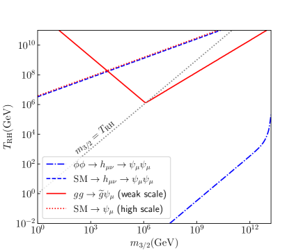
Figure 6: The $(m_{3/2},T_{\rm RH})$ plane showing the contours of $\Omega_{3/2}h^{2}=0.12$. The blue dot-dashed line is derived from the inflaton condensate via single graviton exchange, Eq. (46). The blue dashed line is the thermal contribution from graviton exchange, given by Eq. (59). The red solid line corresponds to single gravitino production when the scale of supersymmetry breaking is below the inflationary scale, Eq. (80), where $m_{1/2}=m_{3/2}$ is assumed. The red dotted line corresponds to the case of high-scale supersymmetry, Eq. (83), where gravitinos must be pair produced.

This thermal bound on $T_{\rm RH}$ is greatly relaxed in models of high scale supersymmetry (shown here by the red dotted line) as single production of gravitinos becomes kinematically forbidden Benakli:2017whb ; grav2 . In this case, from Eq. (83), we see that $\Omega h^{2}\propto T_{\rm RH}^{7}m_{3/2}^{3}$. In contrast, the gravitational production of a stable spin-$\frac{3}{2}$ raritron, whose source is the inflaton, provides a significantly stronger constraint, particularly at low masses. This constraint is shown by the blue dot-dashed line and given by Eq. (46) where $\Omega h^{2}\propto T_{\rm RH}m_{3/2}^{-1}$. As discussed earlier the gravitational production of raritrons from the thermal bath is always sub-dominant. It is shown by the blue dashed line from Eq. (59) and is found extremely close to the line corresponding to the thermal production in high-scale supersymmetry.

This figure is one of the most important results of our studies, and admirably reflects the dominance of gravitational effects over classical thermal gravitino-raritron production, within the parameter space allowed by the unitarity limit, i.e., $m_{3/2}\gtrsim 40$ EeV (non-supersymmetric). However, we caution the reader that the thermal constraints shown here reflect the production of the gravitino in supersymmetric models. The gravitational production of the raritron is definitely not the gravitino in supersymmetry. As we have seen the gravitational production from the inflaton condensate produces primarily the longitudinal component and occurs just after inflation when supersymmetry is broken by the inflationary sector. As a result the longitudinal component is the inflatino and the resulting particles produced are not related to the gravitino at low energies.

IV Summary

Gravitational particle production after inflation is inevitable. All particles couple to gravity through their energy-momentum tensor and can be produced directly from the inflaton condensate during reheating. While it is difficult to create the thermal bath directly from minimal gravitational interactions cmov ; cmo ; Haque:2022kez ; Barman:2022qgt , the production of stable particles making up all or some of the dark matter is feasible MO .

While all particles couple to the inflaton through gravity, they do not couple equally. The production rate, $R$, for particles produced from the condensate are generally proportional to $\rho_{\phi}^{2}$. Since $\rho_{\phi}$ redshifts with the expansion of the Universe as in Eq. (40), and the production rate redshifts faster than the Hubble rate, production occurs at the start of the reheating process. The production of scalars, $S$, is to a good approximation independent of the mass of the scalars when $m_{S}\ll m_{\phi}$ MO ; cmov and absent for massless vectors. However, the production rate for fermions is suppressed due to the necessity of a spin flip for the final state fermion cmov . In this work, we considered the gravitational production of a massive spin-$\frac{3}{2}$ particle dubbed the raritron. We do not however, necessarily associate this particle with the gravitino. As in the case of scalars and spin-$\frac{1}{2}$ fermions, the inflaton couples to raritrons through their respective energy-momentum tensors, $T^{\mu\nu}_{0}$ and $T_{3/2}^{\mu\nu}$.

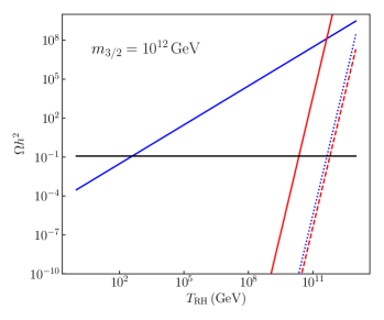
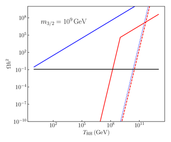
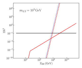
Figure 7: The relic abundance of raritrons/gravitinos, $\Omega h^{2}$ as a function of the reheating temperature for fixed $m_{3/2}=1$ ZeV (upper left panel), $m_{3/2}=1$ EeV (upper right panel), and 1 TeV (lower panel). The blue solid line is derived from Eq. (46) and does not appear in the lower panel due to concerns over unitarity violations. The thermal production of raritrons mediated by gravity is shown as the blue dotted line from Eq. (59). Also shown is the thermal production of gravitinos in both the case of weak-scale (solid red) and high-scale (dotted red) supersymmetry (with $m_{1/2}=m_{3/2}$) taken from Eqs. (80) and (83) respectively. The horizontal black line at $\Omega h^{2}=0.12$ is shown for reference.

As we saw in Fig. 2, the production rate of raritrons is largely dominated by the production of the raritron longitudinal modes, particularly at low raritron masses, as the rate is proportional to $m_{3/2}^{-2}$. This yields a very large abundance of raritrons and unless $m_{3/2}$ is relatively large, the reheating temperature is strongly constrained as we showed in Fig. 3. This result is summarized in Fig. 7 where we show the relic abundance $\Omega h^{2}$ as a function of the reheating temperature for three choices of $m_{3/2}$. The solid blue line is derived from Eq. (46). It is not shown in the lower panel with $m_{3/2}=1$ TeV, as we expect unitarity violations at low masses. We also see in the upper right panel, that even $m_{3/2}=1$ EeV ($10^{9}$ GeV), would require $T_{\rm RH}\lesssim 0.1$ GeV to avoid overproduction. When $m_{3/2}=1$ ZeV ($10^{12}$ GeV), as in the upper left panel, the reheating temperature may be as large as $\sim$ 300 GeV. The horizontal black line is set at $\Omega h^{2}=0.12$ to guide the eye.

Other mechanisms for raritron/gravitino production are also shown in Fig. 7. Note the huge variation in the relic abundance obtained from the different mechanisms. As discussed above, the thermal production of raritrons mediated by gravity is always sub-dominant when compared to the direct production from the inflaton condensate. This source of production is shown by the blue dotted curve in Fig. 7 taken from Eq. (59). Extrapolating to larger masses and reheating temperatures we can see, however, because of the steep dependence ($\Omega h^{2}\propto T_{\rm RH}^{7})$, there are regions where thermal production dominates, but $\Omega h^{2}$ is orders of magnitude too large in this case.

We also show in Fig. 7, the thermal production of gravitinos in both the case of weak-scale (solid red) and high-scale (dotted red) supersymmetry taken from Eqs. (80) and (83) respectively. The abundance of thermally-produced gravitinos in weak–scale scale supersymmetry is proportional to $T_{\rm RH}$ so long as $T_{\rm RH}>m_{3/2}$. As we have already seen in Fig. 6, for large gravitino masses, we must cut off the integration of the Boltzmann equation at $a_{3/2}$ corresponding to the scale factor when $T=m_{3/2}$, rather than integrating down to $a_{\rm RH}$. This leads to a suppression by a factor of $(T_{\rm RH}/m_{3/2})^{6}$. For $m_{3/2}=1$ ZeV, and the parameter range shown in Fig. 7, $T_{\rm RH}<m_{3/2}$ and the we see only the steeper slope. For the other two values of $m_{3/2}$ shown, we see the change in slope when $T_{\rm RH}=m_{3/2}$. For $m_{3/2}=1$ TeV, EeV, ZeV, we have limits of $T_{\rm RH}\lesssim$ $2\times 10^{9}$ GeV, $4\times 10^{7}$ GeV, and $5\times 10^{9}$ GeV respectively to avoid overproduction of gravitinos in weak-scale supersymmetry.

For the case of high-scale supersymmetry, cutting off the integration in the Boltzmann equation only results in a change in the log term in Eq. (83) resulting in a replacement of $T_{\rm RH}$ with $m_{3/2}$ for $T_{\rm RH}<m_{3/2}$. This change is unobservable on the scale shown in the figure. The same is true for the thermal production via gravity in Eq. (59). Since the relic abundance in both cases is $\propto 1/m_{3/2}^{3}$, the heavier the dark matter, the larger the permitted range of $T_{\rm RH}$. The limits in the high-scale supersymmetry cases for $m_{3/2}=1$ TeV, Eev, ZeV, are $T_{\rm RH}\lesssim$ $8\times 10^{7}$ GeV, $3.1\times 10^{10}$ GeV, $6.3\times 10^{11}$ GeV respectively.

We have not included the production of gravitinos from inflatino exchange as that production is suppressed due to mixing with inflatinos. A quantitative measure of the abundance in that case would require an analysis similar to what is done in Nilles:2001fg .

Of course we do not know how dark the dark sector is. At its darkest, gravitational interactions may play a leading role in the production of dark matter. A generic Rarita-Schwinger is easily overproduced in the early Universe through its (minimal) gravitational coupling to the the inflaton. We have derived strong limits on the raritron mass in this case, though depending on the detailed model, unitarity limits may be even stronger. The gravitino in models of broken supersymmetry can also be produced gravitationally, however only the transverse components are produced as the longitudinal states are primarily composed of the inflatino. In this case the standard thermal production of gravitinos still provides limits on its mass and the inflationary reheating temperature.

Appendix A Energy-momentum tensor of spin-3/2 field

In this appendix, we provide a brief review of the computation for the energy-momentum tensor of a spin-$\frac{3}{2}$ particle. We begin with a theory that closely resembles $\mathcal{N}=1$ pure supergravity, where the spin-$\frac{3}{2}$ particle is a Majorana fermion known as the gravitino.

We begin by introducing the full action, which is the sum of the Einstein-Hilbert action and the Rarita-Schwinger action for the massive gravitino,

$$S =\int d^{4}x({\cal L}_{2}+{\cal L}_{3/2})\,,$$ (84)

where

$${\cal L}_{2} =-\frac{M_{P}^{2}}{2}eR\,,$$ (85)

$${\cal L}_{3/2} =-\frac{1}{4}\epsilon^{\mu\nu\rho\sigma}\overline{\psi}_{\mu}\gamma_{5}\gamma_{\nu}\overset{\leftrightarrow}{\nabla}_{\rho}\psi_{\sigma}-\frac{1}{4}em_{3/2}\overline{\psi}_{\mu}[\gamma^{\mu},\gamma^{\nu}]\psi_{\nu}~{}$$

$$=\frac{i}{4}e\overline{\psi}_{\mu}\gamma^{\mu\nu\rho}\overset{\leftrightarrow}{\nabla}_{\rho}\psi_{\nu}-\frac{1}{4}em_{3/2}\overline{\psi}_{\mu}[\gamma^{\mu},\gamma^{\nu}]\psi_{\nu}\,,$$ (86)

with the determinant of the frame field given by $\text{det}~{}e_{\mu}^{a}\equiv e$ and $A\overset{\leftrightarrow}{\nabla}_{\mu}B\equiv A\overset{\rightarrow}{\nabla}_{\mu}B-A\overset{\leftarrow}{\nabla}_{\mu}B$. The covariant derivative acting on the spin-$\frac{3}{2}$ field is defined as

$$\nabla_{\mu}\psi_{\nu} \equiv\left(\partial_{\mu}+\frac{1}{4}\omega_{\mu ab}\gamma^{ab}\right)\psi_{\nu}\,,$$ (87)

$$\overline{\psi}_{\nu}\overset{\leftarrow}{\nabla}_{\mu} =\overline{\psi}_{\nu}\left(\overset{\leftarrow}{\partial}_{\mu}-\frac{1}{4}\omega_{\mu ab}\gamma^{ab}\right)\,,$$ (88)

$$\gamma^{ab} =\gamma^{[a}\gamma^{b]}=\frac{1}{2}[\gamma^{a},\gamma^{b}]\,,$$ (89)

and $\overline{\psi}_{\nu}\overset{\leftarrow}{\partial}_{\mu}\equiv\partial_{\mu}\overline{\psi}_{\nu}$. The frame field $e_{\mu}^{a}$ is related to the flat Minkowski metric as

$$g_{\mu\nu} =e^{a}_{\mu}e^{b}_{\nu}\eta_{ab}\,,$$ (90)

$$\eta_{ab} =\textrm{diag}(+1,-1,-1,-1)\,.$$ (91)

The curvature tensor is given by

$$R_{\mu\nu}{}^{ab} =\partial_{\mu}\omega_{\nu}{}^{ab}-\partial_{\nu}\omega_{\mu}{}^{ab}+\omega_{\mu}{}^{ac}\omega_{\nu c}{}^{b}-\omega_{\nu}{}^{ac}\omega_{\mu c}{}^{b},$$ (92)

$$R_{\mu\nu\rho\sigma} =e_{a\rho}e_{b\sigma}R_{\mu\nu}{}^{ab}\,,$$ (93)

$$R_{\mu\nu} =R^{\rho}{}_{\mu\rho\nu}\,,$$ (94)

$$R =e^{\mu}_{a}e^{\nu}_{b}R_{\mu\nu}{}^{ab}=g^{\mu\nu}R_{\mu\nu}\,,$$ (95)

where $\omega_{\mu ab}$ is the spin connection, given by

$$\omega_{\mu ab}=\omega_{\mu ab}(e)+K_{\mu ab}\,.$$ (96)

Here $K_{\mu\nu\rho}$ is the contorsion tensor and

$$\omega_{\mu}^{ab}(e)=2e^{\nu[a}\partial_{[\mu}e_{\nu]}^{b]}-e^{\nu[a}e^{b]\sigma}e_{\mu c}\partial_{\nu}e_{\sigma}^{c}$$ (97)

is the torsionless contribution. In the non-supersymmetric case, the contorsion can be set to zero. However, in supergravity, $K_{\mu\nu\rho}$ is expressed as a combination of terms bilinear in $\psi_{\mu}$. We derive the energy-momentum tensor $T_{3/2}^{\mu\nu}$ by varying the total Lagrangian ${\cal L}={\cal L}_{2}+{\cal L}_{3/2}$ with respect to the frame field $e$, and then expressing the result in the Minkowski limit $g_{ab}\rightarrow\eta_{ab}$.

The energy-momentum tensor can be derived from the Einstein equation, where the terms other than the pure spin-$2$ contribution are grouped to define $T_{3/2}^{\mu\nu}$. In this context, two main approaches exist: the Palatini and the metric formalism, or the first- and second-order formalism in the context of supergravity. Since it is a quite involved task to compute the energy-momentum tensor using either method, we briefly discuss the distinctions between the two.

In the first-order formalism, the parameters $e$, $\omega$, and $\psi$ (with Lorentz indices suppressed) are treated as independent variables when varying the action. The spin connection $\omega$ is subsequently expressed as a function of $e$ and $\psi$ by requiring $\delta S/\delta\omega=0$ Deser:1976eh . The second-order formalism treats only $e$ and $\psi$ as independent variables, with $\omega$ chosen to ensure that supersymmetry Freedman:1976xh is preserved. This approach assumes Eq. (96) at the starting point. For a more detailed discussion on the first- and second-order formalisms, see Ref. Freedman:2012zz .

In the first-order formalism, the total Lagrangian is treated as a function of $e$, $\omega$, and $\psi$. The solution to $\delta S/\delta\omega=0$ is given by Eq. (96), with $\omega=\omega(e,\psi)$. We then solve the condition $\delta S/\delta e|_{\omega=\omega(e,\psi)}=0$ and find that the Einstein equation is given by

$$\left.G_{\mu\nu}(e,\omega)\right|_{\omega=\omega(e,\psi)}= \displaystyle\frac{e^{-1}e_{\mu a}}{M_{P}}\left.\frac{\delta{\cal L}_{3/2}}{\delta e^{a}_{\nu}}\right|_{\omega=\omega(e,\psi)}\,,$$ (98)

$$G_{\mu\nu}= R_{\mu\nu}-\frac{1}{2}g_{\mu\nu}R\,.$$ (99)

We note that the Einstein tensor $G_{\mu\nu}$ on the left-hand side of Eq. (98) includes both $e$ and $\psi$, the latter due to the contorsion term in the spin connection. Therefore, to derive the correct energy-momentum tensor, the $\psi$-dependent terms must be move to the right-hand side.

On the other hand, in the second-order formalism, deriving the energy-momentum tensor is more straightforward. As the Lagrangian is treated as a function of $e$ and $\psi$, with Eq. (96) already applied to eliminate the explicit $\omega$ dependence, the Einstein equation is simply derived from $\delta{\cal L}/\delta e=0$, and $G_{\mu\nu}$ does not depend on $\psi$. Consequently, the symmetrized energy-momentum tensor is defined as

$$T_{3/2,\mu\nu} =e^{-1}e_{(\mu a}\frac{\delta{\cal L}_{3/2}}{\delta e^{\nu)}_{a}}\,,$$ (100)

where as before ${\cal L}_{3/2}$ is given by eliminating the $\omega$ dependence in the second-order formalism. This approach allows for a direct computation to compute the gravitino energy-momentum tensor, given by

$$T_{3/2,\mu\nu} =-\frac{i}{4}\overline{\psi}_{\rho}\gamma_{(\mu}\overset{\leftrightarrow}{\nabla}_{\nu)}\psi^{\rho}+\frac{i}{2}\overline{\psi}_{(\nu}\gamma_{\mu)}\overset{\leftrightarrow}{\nabla}_{\rho}\psi^{\rho}+\frac{i}{2}\overline{\psi}^{\rho}\gamma_{(\mu}\overset{\leftrightarrow}{\nabla}_{\rho}\psi_{\nu)},$$ (101)

where we have used the equation of motion and the gravitino constraints. We note that the above result does not depend on the gravitino mass. In the flat Minkowski limit, we can replace $\overset{\leftrightarrow}{\nabla}\to\overset{\leftrightarrow}{\partial}$ and neglect the four-Fermi terms originating from the torsion contribution as they are not relevant for our analysis, which leads to Eq. (9).

If we do not assume supersymmetry, the spin-$\frac{3}{2}$ particle is not necessarily a Majorana fermion. For a Dirac spin-$\frac{3}{2}$ particle, the Lagrangian is given by

$${\cal L}_{3/2} =-\frac{1}{2}\epsilon^{\mu\nu\rho\sigma}\overline{\psi}_{\mu}\gamma_{5}\gamma_{\nu}\overset{\leftrightarrow}{\nabla}_{\rho}\psi_{\sigma}-\frac{1}{2}em_{3/2}\overline{\psi}_{\mu}[\gamma^{\mu},\gamma^{\nu}]\psi_{\nu},$$ (102)

and the energy-momentum tensor is given by

$$T_{3/2,\mu\nu}^{\rm(Dirac)} =2T_{3/2,\mu\nu}^{\rm(Majorana)}\,,$$ (103)

where $T_{3/2,\mu\nu}^{\rm(Majorana)}$ is given by Eq. (101).

Appendix B Amplitudes and Thermal Rates

In this appendix, we compute the thermal production rate of raritrons, $R_{\frac{3}{2}}^{T}$. We consider only the massless Standard Model particles in the initial state, which include scalars, fermions, and gauge bosons. The dark matter production rate for the process $\mathrm{SM}+\mathrm{SM}\rightarrow\psi+\psi$ is given by the general expression Eq. (53), where we assumed that $4m_{3/2}^{2}\ll s$ and included a factor of two in the numerator to account that two dark matter particles are produced per scattering event.

We express the squared amplitudes in terms of the Mandelstam variables $s$ and $t$, which are given by

$$t\;=\;\frac{s}{2}\left(\sqrt{1-\frac{4m_{3/2}^{2}}{s}}\cos{\theta_{13}}-1\right)+m_{3/2}^{2}\,,$$ (104)

$$s\;=\;2E_{1}E_{2}(1-\cos{\theta_{12}})\,.$$ (105)

The general squared amplitude for the thermal processes involving SM initial states is given by Eq. (55), where we include $4$ degrees for 1 complex Higgs doublet, $12$ degrees for $8$ gluons and 4 electroweak bosons, and $45$ degrees for 6 (anti)quarks with 3 colors, 3 (anti)charged leptons and 3 neutrinos. We note that the squared amplitudes include the symmetry factors of both the initial and final states, and this is indicated with an overbar.

When summing over all polarizations, the total squared amplitude of the gravity-mediated scalar production of raritrons is given by

$$|\mathcal{\overline{M}}^{0\frac{3}{2}}|^{2}=\frac{1}{72m_{3/2}^{4}M_{P}^{4}s^{2}}\left\{-s^{2}\left(s+2t-2m_{\phi}^{2}\right)^{2}\times\right.$$ (106)

$$\left.\left[m_{\phi}^{4}-2m_{\phi}^{2}t+t(s+t)\right]-72m_{3/2}^{12}+24m_{3/2}^{10}(7s+12t)\right.$$

$$\left.-2m_{3/2}^{8}\left[47s^{2}+264st+216t^{2}+72m_{\phi}^{4}-12m_{\phi}^{2}(s+12t)\right]\right.$$

$$\left.-2m_{3/2}^{6}\left[s^{3}-122s^{2}t-288st^{2}-144t^{3}+12m_{\phi}^{4}(7s-12t)\right.\right.$$

$$\left.\left.+m_{\phi}^{2}\left(288t^{2}+216st-62s^{2}\right)\right]+m_{3/2}^{4}\left[s^{4}-34s^{3}t-210s^{2}t^{2}\right.\right.$$

$$\left.\left.-240st^{3}-72t^{4}-72m_{\phi}^{8}+24m_{\phi}^{6}(s+12t)\right.\right.$$

$$\left.\left.-18m_{\phi}^{4}\left(s^{2}+16st+24t^{2}\right)-4m_{\phi}^{2}\left(s^{3}-35s^{2}t-126st^{2}\right.\right.\right.$$

$$\left.\left.\left.-72t^{3}\right)\right]+m_{3/2}^{2}s\left[24m_{\phi}^{8}+s^{4}+6s^{3}t+44s^{2}t^{2}+64st^{3}\right.\right.$$

$$\left.\left.+24t^{4}-32m_{\phi}^{6}(s+3t)+16m_{\phi}^{4}\left(2s^{2}+8st+9t^{2}\right)\right.\right.$$

$$\left.\left.-2m_{\phi}^{2}\left(5s^{3}+24s^{2}t+80st^{2}+48t^{3}\right)\right]\right.\Bigr{\}}\,,$$

where $m_{\phi}$ is the scalar mass and $m_{3/2}$ is the raritron mass. For the incoming SM Higgs bosons, we set $m_{\phi}=0$, and this expression simplifies to

$$|\mathcal{\overline{M}}^{0\frac{3}{2}}|^{2}=\frac{1}{72m_{3/2}^{4}M_{P}^{4}s^{2}}\left[-s^{2}t(s+t)(s+2t)^{2}-72m_{3/2}^{12}\right.$$ (107)

$$+24m_{3/2}^{10}(7s+12t)-2m_{3/2}^{8}\left(47s^{2}+264st+216t^{2}\right)$$

$$+m_{3/2}^{6}\left(-2s^{3}+244s^{2}t+576st^{2}+288t^{3}\right)$$

$$+m_{3/2}^{4}\left(s^{4}-34s^{3}t-210s^{2}t^{2}-240st^{3}-72t^{4}\right)$$

$$\left.+m_{3/2}^{2}s\left(s^{4}+6s^{3}t+44s^{2}t^{2}+64st^{3}+24t^{4}\right)\right]\,.$$

Similarly, the matrix element squared for the gravity-mediated raritron production from massless fermions is given by

$$|\mathcal{\overline{M}}^{\frac{1}{2}\frac{3}{2}}|^{2}=\frac{1}{144m_{3/2}^{4}M_{P}^{4}s^{2}}\left\{576m_{3/2}^{12}-768m_{3/2}^{10}(s+3t)\right.$$ (108)

$$\left.+4m_{3/2}^{8}\left(137s^{2}+768st+864t^{2}\right)-8m_{3/2}^{6}\left(58s^{3}+265s^{2}t\right.\right.$$

$$\left.\left.+504st^{2}+288t^{3}\right)+4m_{3/2}^{4}\left(13s^{4}+197s^{3}t+513s^{2}t^{2}\right.\right.$$

$$\left.\left.+480st^{3}+144t^{4}\right)+4m_{3/2}^{2}s\left(2s^{4}-31s^{3}t-106s^{2}t^{2}\right.\right.$$

$$\left.\left.-128st^{3}-48t^{4}\right)+s^{2}\left(s^{4}+10s^{3}t+42s^{2}t^{2}\right.\right.$$

$$\left.\left.+64st^{3}+32t^{4}\right)\right\}\,,$$

and the production from massless gauge bosons is given by

$$|\mathcal{\overline{M}}^{1\frac{3}{2}}|^{2}=\frac{1}{18m_{3/2}^{4}M_{P}^{4}s^{2}}\left\{-36m_{3/2}^{12}+12m_{3/2}^{10}(s+12t)\right.$$ (109)

$$\left.-4m_{3/2}^{8}\left(23s^{2}+30st+54t^{2}\right)+4m_{3/2}^{6}\left(3s^{3}+53s^{2}t\right.\right.$$

$$\left.\left.+54st^{2}+36t^{3}\right)-m_{3/2}^{4}\left(25s^{4}+118s^{3}t+186s^{2}t^{2}\right.\right.$$

$$\left.\left.+120st^{3}+36t^{4}\right)+2m_{3/2}^{2}s\left(3s^{4}+7s^{3}t+16s^{2}t^{2}\right.\right.$$

$$\left.\left.+16st^{3}+6t^{4}\right)-s^{2}t(s+t)\left(s^{2}+2st+2t^{2}\right)\right\}\,.$$

By evaluating the integral, we find that the thermal production rate of raritrons can be written as

$$R^{T}_{3/2}\;=\;\beta_{1}\frac{T^{12}}{m_{3/2}^{4}M_{P}^{4}}+\beta_{2}\frac{T^{10}}{m_{3/2}^{2}M_{P}^{4}}+\beta_{3}\frac{T^{8}}{M_{P}^{4}}$$

$$+\beta_{4}\frac{m_{3/2}^{2}T^{6}}{M_{P}^{4}}+\beta_{5}\frac{m_{3/2}^{4}T^{4}}{M_{P}^{4}}\,,$$ (110)

where

$$\beta_{1}\;=\;\frac{205511\pi^{7}}{85730400}\,,$$ (111)

$$\beta_{2}\;=\;\frac{16453\zeta(5)^{2}}{15\pi^{5}}\,,$$ (112)

$$\beta_{3}\;=\;-\frac{369149\pi^{3}}{93312000}\,,$$ (113)

$$\beta_{4}\;=\;-\frac{8759\zeta(3)^{2}}{1152\pi^{5}}\,,$$ (114)

$$\beta_{5}\;=\;-\frac{49}{5760\pi}\,.$$ (115)

Appendix C Computation of the gravitino production rate

The production rate of the gravitino can be derived from the energy transfer rate from the inflaton energy density $\rho_{\phi}$ to the gravitino sector. Using the equation of state parameter $w_{\phi}=p_{\phi}/\rho_{\phi}$ for the inflaton, the evolution of $\rho_{\phi}$ follows

$$\frac{d\rho_{\phi}}{dt}+3H(1+w_{\phi})\rho_{\phi}\;=\;-(1+w_{\phi})\Gamma_{\phi}\rho_{\phi}\,,$$ (116)

where the right-hand side is given by the energy transfer per space-time volume (Vol₄) due to the inflaton decay or scattering processes to particles $A$ and $B$, defined as

$$(1+w_{\phi})\Gamma_{\phi}\rho_{\phi}\;\equiv\;\frac{\Delta E}{{\rm Vol}_{4}}\,,$$ (117)

where

$$\Delta E \equiv \int\frac{d^{3}p_{A}}{(2\pi)^{3}2p_{A}^{0}}\frac{d^{3}p_{B}}{(2\pi)^{3}2p_{B}^{0}}(p_{A}^{0}+p_{B}^{0})$$

$$\times \left|\frac{1}{n!}\biggl{<}{\rm f}\left|\left(i\int d^{4}x_{1}{\cal L}_{\rm int}\right)\cdots\left(i\int d^{4}x_{n}{\cal L}_{\rm int}\right)\right|0\biggr{>}\right|^{2},$$

and ${\cal L}_{\rm int}$ is the interaction Lagrangian  (see GKMO2 for more details).

We decompose the oscillating inflaton as $\phi(t)\simeq\phi_{0}(t){\cal P}(t)$, where ${\cal P}$ represents the rapidly oscillating component and $\phi_{0}$ is its envelope that slowly evolves (redshifts) with time. In practice, $\phi_{0}$ can be taken as a constant quantity when computing a reaction that occurs over time scales much shorter than the change in $\phi_{0}$. Therefore, the fast oscillating component can be decomposed as

$${\cal P}(t)\;=\;\sum_{n=-\infty}^{\infty}{\cal P}_{n}e^{-in\omega t}\,,$$ (119)

where $\omega$ is the frequency of the inflaton oscillation.

Using the interaction Lagrangian ${\cal L}_{\rm int}$, given by Eq. (LABEL:eq:L_gravitino), the amplitudes for the $t$- and $u$-channels are given by

$${\cal M}^{(n,m)}_{t} = \frac{1}{4M_{P}^{2}}\frac{nm{\cal P}_{n}{\cal P}_{m}}{t_{n}-m_{\chi}^{2}}(\omega\phi_{0})^{2}\bar{u}_{\mu}(p_{A})\not{\delta}\gamma^{\mu}(\not{p}_{\phi,n}-\not{p}_{A})\gamma^{\nu}\not{\delta}P_{R}u_{\nu}^{c}(p_{B})\,,$$ (120)

$${\cal M}^{(n,m)}_{u} = \frac{1}{4M_{P}^{2}}\frac{nm{\cal P}_{n}{\cal P}_{m}}{u_{n}-m_{\chi}^{2}}(\omega\phi_{0})^{2}\bar{u}_{\mu}(p_{A})\not{\delta}\gamma^{\mu}(\not{p}_{B}-\not{p}_{\phi,n})\gamma^{\nu}\not{\delta}P_{L}u_{\nu}^{c}(p_{B})\,,$$ (121)

where $p_{\phi,n}^{\mu}=(n\omega,\vec{0})^{\mu}$, $t_{n}\equiv(p_{\phi,n}-p_{A})^{2}$, $u_{n}\equiv(p_{B}-p_{\phi,n})^{2}$, and $\not{\delta}\equiv\delta^{0}_{\mu}\gamma^{\mu}$ is introduced to account for $\partial_{\mu}\phi=(\dot{\phi},\vec{0})_{\mu}$. Using these amplitudes, the energy transfer rate can be written as

$$\frac{\Delta E}{{\rm Vol}_{4}} = \int\frac{d^{3}p_{A}}{(2\pi)^{3}2p_{A}^{0}}\frac{d^{3}p_{B}}{(2\pi)^{3}2p_{B}^{0}}(p_{A}^{0}+p_{B}^{0})\sum_{n+m>0}\sum_{\rm spin}|{\cal M}_{t}^{(n,m)}+{\cal M}_{u}^{(n,m)}|^{2}(2\pi)^{4}\delta^{4}(p_{\phi,n}+p_{\phi,m}-p_{A}-p_{B})\,.$$ (122)

If we use the equation of motion for $\psi_{\mu}$, the sum of the amplitudes greatly simplifies and becomes

$${\cal M}_{t}^{(n,m)}+{\cal M}_{u}^{(n,m)} =\frac{m_{3/2}}{M_{P}^{2}}\frac{nm{\cal P}_{n}{\cal P}_{m}}{nm\omega^{2}+m_{\chi}^{2}-m_{3/2}^{2}}$$

$$\times(\omega\phi_{0})^{2}\delta^{\mu}_{0}\delta^{\nu}_{0}\bar{u}_{\mu}(p_{A})u_{\nu}^{c}(p_{B})\,,$$ (123)

where we used $t_{n}=u_{n}=m_{3/2}^{2}-nm\omega^{2}$ and $p_{A}^{0}=p_{B}^{0}=(n+m)\omega/2$. We emphasize that only the $\mu=0$ contribution of $\psi_{\mu}$ is produced. The gravitino wave function may be written as $\psi_{\mu}\sim\psi\epsilon_{\mu}$, where $\psi$ and $\epsilon_{\mu}$ denote the spin-$\frac{1}{2}$ and 1 components, respectively. It is important to note that the spin $\pm$3/2 component is proportional to the transverse polarization of $\epsilon_{\mu}$, which does not have the $\mu=0$ component. As a result, only spin $\pm$1/2 mode of the gravitino may have a nonzero amplitude.

Thus, the amplitude given by Eq. (123) can be further simplified by substituting $u_{0}(p)=\sqrt{2/3}\epsilon_{0}(p)u(p)=\sqrt{2/3}(|\vec{p}|/m_{3/2})u(p)$, where $u(p)$ is the spin-$\frac{1}{2}$ component that satisfies $(\not{p}-m_{3/2})u(p)=0$. Without specifying the oscillatory solution of the inflaton, we derive obtain the energy transfer rate:

$$(1+w_{\phi})\Gamma_{\phi\phi\to\psi_{\mu}\psi_{\mu}}\rho_{\phi}=\sum_{n+m\geq 1}\frac{(nm)^{2}(n+m)^{7}({\cal P}_{n}{\cal P}_{m})^{2}\omega^{11}\phi_{0}^{4}}{144\pi m_{3/2}^{2}M_{P}^{4}(nm\omega^{2}+m_{\chi}^{2}-m_{3/2}^{2})^{2}}\left(1-\frac{4m_{3/2}^{2}}{(n+m)^{2}\omega^{2}}\right)^{7/2}\,.$$ (124)

For concreteness, we consider $V(\phi)=(m_{\phi}^{2}/2)\phi^{2}$, which implies that $w_{\phi}=0$. The solution for $\phi$ can be expressed as $\phi(t)\simeq\phi_{0}(t)\cos(\omega t)$, where $\omega=m_{\phi}$ and $\rho_{\phi}\simeq(m_{\phi}^{2}/2)\phi_{0}^{2}$. Consequently, ${\cal P}_{n=\pm 1}=1/2$, and is zero otherwise. Therefore, only the $n=m=1$ modes contribute, and we obtain

$$\Gamma_{\phi\phi\to\psi_{\mu}\psi_{\mu}} = \frac{2m_{\phi}\rho_{\phi}}{9\pi M_{P}^{4}}\frac{(1-\tau_{3/2})^{7/2}}{\tau_{3/2}(1+\tau_{\chi}-\tau_{3/2})^{2}}\,.$$ (125)

where $\tau_{i}\equiv m_{i}^{2}/m_{\phi}^{2}$.

References

- (1) K. A. Olive, Phys. Rept. 190 (1990) 307; A. D. Linde, Particle Physics and Inflationary Cosmology (Harwood, Chur, Switzerland, 1990); D. H. Lyth and A. Riotto, Phys. Rep. 314 (1999) 1 [arXiv:hep-ph/9807278]; J. Martin, C. Ringeval and V. Vennin, Phys. Dark Univ. 5-6, 75-235 (2014) [arXiv:1303.3787 [astro-ph.CO]]; J. Martin, C. Ringeval, R. Trotta and V. Vennin, JCAP 1403 (2014) 039 [arXiv:1312.3529 [astro-ph.CO]]; J. Martin, Astrophys. Space Sci. Proc. 45, 41 (2016) [arXiv:1502.05733 [astro-ph.CO]].
- (2) N. Aghanim et al. [Planck], Astron. Astrophys. 641, A6 (2020) [arXiv:1807.06209 [astro-ph.CO]].
- (3) A. D. Dolgov and A. D. Linde, Phys. Lett. 116B, 329 (1982); L. F. Abbott, E. Farhi and M. B. Wise, Phys. Lett. 117B, 29 (1982).
- (4) D. V. Nanopoulos, K. A. Olive and M. Srednicki, Phys. Lett. B 127, 30 (1983).
- (5) G. F. Giudice, E. W. Kolb and A. Riotto, Phys. Rev. D 64 (2001) 023508 [hep-ph/0005123]; D. J. H. Chung, E. W. Kolb and A. Riotto, Phys. Rev. D 60 (1999) 063504 [hep-ph/9809453].
- (6) M. A. G. Garcia, Y. Mambrini, K. A. Olive and M. Peloso, Phys. Rev. D 96, no.10, 103510 (2017) [arXiv:1709.01549 [hep-ph]].
- (7) N. Bernal, JCAP 10, 006 (2020) [arXiv:2005.08988 [hep-ph]]; A. Di Marco and G. Pradisi, Int. J. Mod. Phys. A 36, no.15, 2150095 (2021) [arXiv:2102.00326 [gr-qc]].
- (8) M. A. G. Garcia, K. Kaneta, Y. Mambrini and K. A. Olive, Phys. Rev. D 101 (2020) no.12, 123507 [arXiv:2004.08404 [hep-ph].
- (9) M. A. G. Garcia, K. Kaneta, Y. Mambrini and K. A. Olive, JCAP 04, 012 (2021) [arXiv:2012.10756 [hep-ph]].
- (10) M. Becker, E. Copello, J. Harz, J. Lang and Y. Xu, [arXiv:2306.17238 [hep-ph]].
- (11) L. J. Hall, K. Jedamzik, J. March-Russell and S. M. West, JHEP 1003 (2010) 080 [arXiv:0911.1120 [hep-ph]]; X. Chu, T. Hambye and M. H. G. Tytgat, JCAP 1205 (2012) 034 [arXiv:1112.0493 [hep-ph]]; A. Biswas, D. Borah and A. Dasgupta, Phys. Rev. D 99, no.1, 015033 (2019) [arXiv:1805.06903 [hep-ph]].
- (12) Y. Mambrini, K. A. Olive, J. Quevillon and B. Zaldivar, Phys. Rev. Lett. 110, no.24, 241306 (2013) [arXiv:1302.4438 [hep-ph]].
- (13) J. R. Ellis, J. S. Hagelin, D. V. Nanopoulos, K. A. Olive and M. Srednicki, Nucl. Phys. B 238, 453 (1984).
- (14) M. Y. Khlopov and A. D. Linde, Phys. Lett. B 138, 265 (1984).
- (15) J. R. Ellis, J. E. Kim and D. V. Nanopoulos, Phys. Lett. B 145, 181 (1984).
- (16) K. A. Olive, D. N. Schramm and M. Srednicki, Nucl. Phys. B 255, 495 (1985).
- (17) X. Chu, Y. Mambrini, J. Quevillon and B. Zaldivar, JCAP 1401 (2014) 034 [arXiv:1306.4677 [hep-ph]]; G. Bhattacharyya, M. Dutra, Y. Mambrini and M. Pierre, Phys. Rev. D 98 (2018) no.3, 035038 [arXiv:1806.00016 [hep-ph]]; A. Banerjee, G. Bhattacharyya, D. Chowdhury and Y. Mambrini, JCAP 12 (2019), 009 [arXiv:1905.11407 [hep-ph]].
- (18) N. Bernal, M. Heikinheimo, T. Tenkanen, K. Tuominen and V. Vaskonen, Int. J. Mod. Phys. A 32 (2017) no.27, 1730023 [arXiv:1706.07442 [hep-ph]].
- (19) N. Bernal, JCAP 10, 006 (2020) [arXiv:2005.08988 [hep-ph]]; N. Bernal, J. Rubio and H. Veermäe, JCAP 10, 021 (2020) [arXiv:2006.02442 [hep-ph]].
- (20) N. Bernal, F. Elahi, C. Maldonado and J. Unwin, JCAP 11 (2019), 026 [arXiv:1909.07992 [hep-ph]].
- (21) B. Barman, D. Borah and R. Roshan, JCAP 11, 021 (2020) [arXiv:2007.08768 [hep-ph]].
- (22) S. L. Chen and Z. Kang, JCAP 05, 036 (2018) [arXiv:1711.02556 [hep-ph]]; A. Ahmed and S. Najjari, [arXiv:2112.14261 [hep-ph]].
- (23) J. Ellis, M. A. G. Garcia, D. V. Nanopoulos, K. A. Olive and M. Peloso, JCAP 1603, no. 03, 008 (2016) [arXiv:1512.05701 [astro-ph.CO]].
- (24) E. Dudas, Y. Mambrini and K. Olive, Phys. Rev. Lett. 119 (2017) no.5, 051801 [arXiv:1704.03008 [hep-ph]].
- (25) K. Kaneta, Y. Mambrini and K. A. Olive, Phys. Rev. D 99 (2019) no.6, 063508 [arXiv:1901.04449 [hep-ph]].
- (26) Y. Mambrini, K. A. Olive and J. Zheng, JCAP 10, 055 (2022) [arXiv:2208.05859 [hep-ph]].
- (27) Y. Ema, R. Jinno, K. Mukaida and K. Nakayama, JCAP 05, 038 (2015) [arXiv:1502.02475 [hep-ph]]; Y. Ema, R. Jinno, K. Mukaida and K. Nakayama, Phys. Rev. D 94, no.6, 063517 (2016) [arXiv:1604.08898 [hep-ph]]; Y. Ema, K. Nakayama and Y. Tang, JHEP 09, 135 (2018) [arXiv:1804.07471 [hep-ph]].
- (28) M. Garny, M. Sandora and M. S. Sloth, Phys. Rev. Lett. 116, no.10, 101302 (2016) [arXiv:1511.03278 [hep-ph]]; M. Garny, A. Palessandro, M. Sandora and M. S. Sloth, JCAP 02, 027 (2018) [arXiv:1709.09688 [hep-ph]].
- (29) Y. Tang and Y. L. Wu, Phys. Lett. B 774, 676-681 (2017) [arXiv:1708.05138 [hep-ph]].
- (30) N. Bernal, M. Dutra, Y. Mambrini, K. Olive, M. Peloso and M. Pierre, Phys. Rev. D 97 (2018) no.11, 115020 [arXiv:1803.01866 [hep-ph]].
- (31) M. Chianese, B. Fu and S. F. King, JCAP 06, 019 (2020) [arXiv:2003.07366 [hep-ph]]; M. Chianese, B. Fu and S. F. King, JCAP 01, 034 (2021) [arXiv:2009.01847 [hep-ph]].
- (32) M. Redi, A. Tesi and H. Tillim, JHEP 05, 010 (2021) [arXiv:2011.10565 [hep-ph]].
- (33) Y. Mambrini and K. A. Olive, Phys. Rev. D 103 (2021) no.11, 115009 [arXiv:2102.06214 [hep-ph]].
- (34) B. Barman and N. Bernal, JCAP 06, 011 (2021) [arXiv:2104.10699 [hep-ph]].
- (35) A. Ahmed, B. Grzadkowski and A. Socha, Phys. Lett. B 831, 137201 (2022) [arXiv:2111.06065 [hep-ph]].
- (36) N. Bernal and C. S. Fong, JCAP 06 (2021), 028 doi:10.1088/1475-7516/2021/06/028 [arXiv:2103.06896 [hep-ph]]; X. Sun, [arXiv:2112.04304 [hep-ph]].
- (37) M. R. Haque and D. Maity, Phys. Rev. D 106, no.2, 023506 (2022) [arXiv:2112.14668 [hep-ph]].
- (38) S. Clery, Y. Mambrini, K. A. Olive and S. Verner, Phys. Rev. D 105, no.7, 075005 (2022) [arXiv:2112.15214 [hep-ph]].
- (39) M. R. Haque and D. Maity, Phys. Rev. D 107, no.4, 043531 (2023) [arXiv:2201.02348 [hep-ph]].
- (40) S. Aoki, H. M. Lee, A. G. Menkara and K. Yamashita, JHEP 05, 121 (2022) [arXiv:2202.13063 [hep-ph]].
- (41) S. Clery, Y. Mambrini, K. A. Olive, A. Shkerin and S. Verner, Phys. Rev. D 105, no.9, 095042 (2022) [arXiv:2203.02004 [hep-ph]].
- (42) R. T. Co, Y. Mambrini and K. A. Olive, Phys. Rev. D 106, no.7, 075006 (2022) [arXiv:2205.01689 [hep-ph]].
- (43) A. Ahmed, B. Grzadkowski and A. Socha, JHEP 02, 196 (2023) [arXiv:2207.11218 [hep-ph]].
- (44) B. Barman, S. Cléry, R. T. Co, Y. Mambrini and K. A. Olive, JHEP 12, 072 (2022) [arXiv:2210.05716 [hep-ph]].
- (45) M. R. Haque, D. Maity and R. Mondal, JHEP 09, 012 (2023) [arXiv:2301.01641 [hep-ph]].
- (46) K. Kaneta, S. M. Lee and K. y. Oda, JCAP 09, 018 (2022) doi:10.1088/1475-7516/2022/09/018 [arXiv:2206.10929 [astro-ph.CO]].
- (47) K. Kaneta and K. y. Oda, [arXiv:2304.12578 [hep-ph]].
- (48) M. A. G. Garcia, M. Pierre and S. Verner, [arXiv:2305.14446 [hep-ph]].
- (49) M. A. G. Garcia, Y. Mambrini, K. A. Olive and S. Verner, Phys. Rev. D 102, no.8, 083533 (2020) [arXiv:2006.03325 [hep-ph]].
- (50) G. Velo and D. Zwanziger, Phys. Rev. 186 (1969), 1337-1341
- (51) A. K. Das and D. Z. Freedman, Nucl. Phys. B 114 (1976), 271-296
- (52) S. Deser and A. Waldron, Nucl. Phys. B 631, 369-387 (2002) [arXiv:hep-th/0112182 [hep-th]].
- (53) M. Fierz and W. Pauli, Proc. Roy. Soc. Lond. A 173 (1939), 211-232
- (54) W. Rarita and J. Schwinger, Phys. Rev. 60 (1941), 61
- (55) Y. Mambrini, Particles in the dark Universe, Springer Ed., ISBN 978-3-030-78139-2 (2021).
- (56) B. R. Holstein, Am. J. Phys. 74, 1002-1011 (2006) [arXiv:gr-qc/0607045 [gr-qc]].
- (57) A. K. Das, Phys. Rev. D 18 (1978), 2065; K. Benakli, Y. Chen, P. Cheng and G. Lafforgue-Marmet, Phys. Rev. D 99, no.9, 095032 (2019) [arXiv:1811.11774 [hep-ph]]; K. Benakli, Int. J. Mod. Phys. A 35 (2020) no.36, 2044029 [arXiv:2004.14770 [hep-ph]]; G. Y. Prokhorov, O. V. Teryaev and V. I. Zakharov, Phys. Rev. D 106, no.2, 025022 (2022) [arXiv:2202.02168 [hep-th]].
- (58) A. A. Starobinsky, Phys. Lett. B 91, 99 (1980).
- (59) R. Kallosh and A. Linde, JCAP 07, 002 (2013) [arXiv:1306.5220 [hep-th]].
- (60) H. Haberzettl, [arXiv:nucl-th/9812043 [nucl-th]].
- (61) R. Ding and Y. Liao, JHEP 04, 054 (2012) [arXiv:1201.0506 [hep-ph]].
- (62) K. Ichikawa, T. Suyama, T. Takahashi and M. Yamaguchi, Phys. Rev. D 78 (2008), 063545 [arXiv:0807.3988 [astro-ph]].
- (63) K. Kainulainen, S. Nurmi, T. Tenkanen, K. Tuominen and V. Vaskonen, JCAP 06 (2016), 022 [arXiv:1601.07733 [astro-ph.CO]].
- (64) J. L. Diaz-Cruz and B. O. Larios, J. Phys. G 45, no.1, 015002 (2018) [arXiv:1612.04331 [hep-ph]].
- (65) J. Ellis, M. A. G. Garcia, D. V. Nanopoulos, K. A. Olive and S. Verner, Phys. Rev. D 105 (2022) no.4, 043504 [arXiv:2112.04466 [hep-ph]].
- (66) I. Antoniadis, A. Guillen and F. Rondeau, JHEP 01, 043 (2023) [arXiv:2210.00817 [hep-th]].
- (67) K. Benakli, Y. Chen, E. Dudas and Y. Mambrini, Phys. Rev. D 95, no.9, 095002 (2017) [arXiv:1701.06574 [hep-ph]].
- (68) J. R. Ellis, J. E. Kim and D. V. Nanopoulos, Phys. Lett. B 145, 181 (1984); T. Moroi, hep-ph/9503210, J. R. Ellis, D. V. Nanopoulos, K. A. Olive and S. J. Rey, Astropart. Phys. 4, 371 (1996) [hep-ph/9505438]; M. Bolz, A. Brandenburg and W. Buchmuller, Nucl. Phys. B 606, 518 (2001) [Erratum-ibid. B 790, 336 (2008)] [hep-ph/0012052]; R. H. Cyburt, J. Ellis, B. D. Fields and K. A. Olive, Phys. Rev. D 67, 103521 (2003) [astro-ph/0211258]; F. D. Steffen, JCAP 0609, 001 (2006) [hep-ph/0605306]; J. Pradler and F. D. Steffen, Phys. Rev. D 75, 023509 (2007) [hep-ph/0608344]; V. S. Rychkov and A. Strumia, Phys. Rev. D 75, 075011 (2007) [hep-ph/0701104]; M. Kawasaki, K. Kohri, T Moroi and A.Yotsuyanagi, Phys. Rev. D 78, 065011 (2008) [arXiv:0804.3745 [hep-ph]]; H. Eberl, I. D. Gialamas and V. C. Spanos, Phys. Rev. D 103, no.7, 075025 (2021) [arXiv:2010.14621 [hep-ph]].
- (69) G. F. Giudice, A. Riotto and I. Tkachev, JHEP 9911, 036 (1999) [hep-ph/9911302];
- (70) R. Kallosh, L. Kofman, A. D. Linde and A. Van Proeyen, Phys. Rev. D 61, 103503 (2000) [arXiv:hep-th/9907124 [hep-th]].
- (71) G. F. Giudice, I. Tkachev and A. Riotto, JHEP 08, 009 (1999) [arXiv:hep-ph/9907510 [hep-ph]].
- (72) R. Kallosh, L. Kofman, A. D. Linde and A. Van Proeyen, Class. Quant. Grav. 17, 4269-4338 (2000) [erratum: Class. Quant. Grav. 21, 5017 (2004)] [arXiv:hep-th/0006179 [hep-th]].
- (73) H. P. Nilles, M. Peloso and L. Sorbo, Phys. Rev. Lett. 87, 051302 (2001) [arXiv:hep-ph/0102264 [hep-ph]].
- (74) H. P. Nilles, M. Peloso and L. Sorbo, JHEP 04, 004 (2001) [arXiv:hep-th/0103202 [hep-th]].
- (75) Y. Ema, K. Mukaida, K. Nakayama and T. Terada, JHEP 11, 184 (2016) [arXiv:1609.04716 [hep-ph]].
- (76) H. P. Nilles, K. A. Olive and M. Peloso, Phys. Lett. B 522, 304-314 (2001) [arXiv:hep-ph/0107212 [hep-ph]].
- (77) K. Benakli, L. Darmé and Y. Oz, JHEP 10, 121 (2014) [arXiv:1407.8321 [hep-ph]].
- (78) F. Hasegawa, K. Mukaida, K. Nakayama, T. Terada and Y. Yamada, Phys. Lett. B 767, 392-397 (2017) [arXiv:1701.03106 [hep-ph]].
- (79) E. W. Kolb, A. J. Long and E. McDonough, Phys. Rev. D 104, no.7, 075015 (2021) [arXiv:2102.10113 [hep-th]]; E. W. Kolb, A. J. Long and E. McDonough, Phys. Rev. Lett. 127, no.13, 131603 (2021) [arXiv:2103.10437 [hep-th]].
- (80) E. Dudas, M. A. G. Garcia, Y. Mambrini, K. A. Olive, M. Peloso and S. Verner, Phys. Rev. D 103, 123519 (2021) [arXiv:2104.03749 [hep-th]].
- (81) T. Terada, Phys. Rev. D 103, no.12, 125022 (2021) [arXiv:2104.05731 [hep-th]].
- (82) I. Antoniadis, K. Benakli and W. Ke, JHEP 11, 063 (2021) [arXiv:2105.03784 [hep-th]].
- (83) J. R. Ellis, C. Kounnas and D. V. Nanopoulos, Phys. Lett. 143B, 410 (1984).
- (84) M. Dine, R. Kitano, A. Morisse and Y. Shirman, Phys. Rev. D 73, 123518 (2006) [hep-ph/0604140]; R. Kitano, Phys. Lett. B 641, 203 (2006) [hep-ph/0607090]; R. Kallosh and A. D. Linde, JHEP 0702, 002 (2007) [hep-th/0611183]; H. Abe, T. Higaki and T. Kobayashi, Phys. Rev. D 76 (2007) 105003 [arXiv:0707.2671 [hep-th]]; J. Fan, M. Reece and L.-T. Wang, JHEP 1109, 126 (2011) [arXiv:1106.6044 [hep-ph]]; Y. Ema, R. Kitano and T. Terada, JHEP 09, 075 (2018) [arXiv:1807.06940 [hep-th]].
- (85) E. Dudas, A. Linde, Y. Mambrini, A. Mustafayev and K. A. Olive, Eur. Phys. J. C 73 (2013) 2268 [arXiv:1209.0499 [hep-ph]].
- (86) M. A. G. García and K. A. Olive, JCAP 1309, 007 (2013) [arXiv:1306.6119 [hep-ph]].
- (87) J. L. Evans, M. A. G. García and K. A. Olive, JCAP 1403, 022 (2014) [arXiv:1311.0052 [hep-ph]].
- (88) E. Dudas, T. Gherghetta, Y. Mambrini and K. A. Olive, Phys. Rev. D 96, no. 11, 115032 (2017) [arXiv:1710.07341 [hep-ph]];
- (89) K. Kaneta, Y. Mambrini, K. A. Olive and S. Verner, Phys. Rev. D 101, no. 1, 015002 (2020) [arXiv:1911.02463 [hep-ph]].
- (90) E. Cremmer, S. Ferrara, C. Kounnas and D. V. Nanopoulos, Phys. Lett. B 133 (1983) 61; A. B. Lahanas and D. V. Nanopoulos, Phys. Rept. 145 (1987) 1.
- (91) J. Ellis, D. V. Nanopoulos and K. A. Olive, JCAP 10, 009 (2013) [arXiv:1307.3537 [hep-th]].
- (92) J. Ellis, M. A. G. Garcia, D. V. Nanopoulos and K. A. Olive, JCAP 10, 003 (2015) [arXiv:1503.08867 [hep-ph]].
- (93) J. Ellis, D. V. Nanopoulos, K. A. Olive and S. Verner, JCAP 08, 037 (2020) [arXiv:2004.00643 [hep-ph]].
- (94) J. Ellis, M. A. G. Garcia, N. Nagata, N. D. V., K. A. Olive and S. Verner, Int. J. Mod. Phys. D 29, no.16, 2030011 (2020) [arXiv:2009.01709 [hep-ph]].
- (95) M. Endo, K. Kadota, K. A. Olive, F. Takahashi and T. T. Yanagida, JCAP 02, 018 (2007) [arXiv:hep-ph/0612263 [hep-ph]].
- (96) R. Kallosh, A. Linde, K. A. Olive and T. Rube, Phys. Rev. D 84, 083519 (2011) [arXiv:1106.6025 [hep-th]].
- (97) T. Terada, Y. Watanabe, Y. Yamada and J. Yokoyama, JHEP 02, 105 (2015) [arXiv:1411.6746 [hep-ph]].
- (98) E. Dudas, T. Gherghetta, K. Kaneta, Y. Mambrini and K. A. Olive, Phys. Rev. D 98, no.1, 015030 (2018) [arXiv:1805.07342 [hep-ph]].
- (99) S. Cecotti, Phys. Lett. B 190 (1987) 86.
- (100) S. Ferrara, A. Kehagias and A. Riotto, Fortsch. Phys. 62, 573 (2014) [arXiv:1403.5531 [hep-th]]; S. Ferrara, A. Kehagias and A. Riotto, Fortsch. Phys. 63, 2 (2015) [arXiv:1405.2353 [hep-th]]; R. Kallosh, A. Linde, B. Vercnocke and W. Chemissany, JCAP 1407, 053 (2014) [arXiv:1403.7189 [hep-th]]; K. Hamaguchi, T. Moroi and T. Terada, Phys. Lett. B 733, 305 (2014) [arXiv:1403.7521 [hep-ph]]; J. Ellis, M. A. G. García, D. V. Nanopoulos and K. A. Olive, JCAP 1405, 037 (2014) [arXiv:1403.7518 [hep-ph]];
- (101) J. Ellis, M. A. G. Garcia, D. V. Nanopoulos and K. A. Olive, JCAP 08, 044 (2014) [arXiv:1405.0271 [hep-ph]].
- (102) J. Ellis, M. A. G. Garcia, D. V. Nanopoulos and K. A. Olive, JCAP 07, 050 (2015) [arXiv:1505.06986 [hep-ph]].
- (103) J. Polonyi, Budapest preprint KFKI-1977-93 (1977).
- (104) S. Deser and B. Zumino, Phys. Lett. B 62, 335 (1976)
- (105) D. Z. Freedman, P. van Nieuwenhuizen and S. Ferrara, Phys. Rev. D 13, 3214-3218 (1976)
- (106) D. Z. Freedman and A. Van Proeyen, Cambridge Univ. Press, 2012, ISBN 978-1-139-36806-3, 978-0-521-19401-3