Triage of the Gaia DR3 astrometric orbits. II. A census of white dwarfs

Abstract

The third data release of Gaia was the first to include orbital solutions assuming non-single stars. Here, we apply the astrometric triage technique of Shahaf et al. 2019 to identify binary star systems with companions that are not single main-sequence stars. Gaia’s synthetic photometry of these binaries is used to distinguish between systems likely to have white-dwarf companions and those that may be hierarchical triples. The study uncovered a population of nearly $3\,200$ binaries, characterised by orbital separations on the order of an astronomical unit, in which the faint astrometric companion is probably a white dwarf. Remarkably, over $110$ of these systems exhibit significant ultraviolet excess flux, confirming this classification and, in some cases, indicating their relatively young cooling ages. We show that the sample is not easily reproduced by binary population synthesis codes. Therefore, it challenges current binary evolution models, offering a unique opportunity to gain insights into the processes governing white-dwarf formation, binary evolution, and mass transfer.

1 Introduction

The detection of white dwarfs (WDs) in wide binaries goes back to the early days of modern astrometry, when in 1844 Friedrich Bessel reported on peculiar changes in the sky position of Sirius and Procyon. After considering several possibilities, Bessel concluded that Sirius and Procyon are not single stars and move under the gravitational force induced by unseen companions of unknown nature. The proximity of Sirius and Procyon to Earth eventually allowed for direct imaging of these faint companions (Bond, 1862; Schaeberle, 1896), and led to their identification as WDs.

The detection of WDs in binaries that are located at distances considerably greater than that of Sirius and Procyon relies on the indirect method initially proposed by Bessel—detecting the faint WD through its effect on the orbital motion of its visibly brighter, usually main-sequence (MS), primary star. However, the analysis of the binary motion alone is often insufficient to determine the nature of the faint companion. Traditionally, identifying WD companions has depended on observing their contributions to the system’s brightness in short-wavelength bands (e.g. Parsons et al., 2016, and references therein). The flux ratio between the WD companions and their bright stars can sometimes be detected in those bands, as the WDs can be much hotter than their companions.

Still, in many cases, the light contribution of the WD is too small to be detected, even in the short-wavelength bands. Therefore, it is likely that many WD companions to MS stars eluded detection or were incorrectly classified (Holberg et al., 2013), particularly if their MS companion is of spectral type earlier than M0.

This situation has changed drastically with the release of a catalogue of nearly $170\,000$ astrometric binaries, many of which are presumed to have unseen WD companions, in the third data release (DR3) of Gaia (Gaia Collaboration, Arenou, et al. 2022). Compact companions in such systems can be identified by ruling out all other possibilities. These include a relatively faint single MS companion or, in case the observed binary is wide enough, a companion that is by itself a short-period binary consisting of two faint MS stars (e.g. Shahaf et al., 2019; Shenar et al., 2022; Janssens et al., 2022; Shahaf et al., 2023; El-Badry et al., 2023). Obtaining a large sample of binaries with WD secondaries may refine our understanding of the late stages of stellar evolution of the binary population, the WD initial-to-final mass relation, and the processes governing mass transfer and co-evolution in binary systems (Gratton et al. 2021; Venner et al. 2023; Escorza & De Rosa 2023; Zhang et al. 2023a; Sayeed et al. 2023).

The first paper of this series, Shahaf et al. (2023, Paper I henceforth), identified the astrometric binaries that are most unlikely to have single MS companions. Based on this classification, the work presented here divides those binaries into two sub-groups: those whose companions are likely to be short-period faint MS binaries by themselves (i.e., hierarchical triple systems) and those that probably have WD companions. The division between these two sub-groups is done by identifying the light contribution of the faint companion(s). Instead of searching for the short-wavelength contribution from the WD, we utilise the availability of Gaia’s synthetic photometry to identify the long-wavelength contribution of faint MS close-binary companions. We assume that the binaries with no long-wavelength excess are the ones with WD companions.

The structure of this paper is as follows: In Section 2, we outline the process we used to select our sample and provide a review of its characteristics. Section 3 discusses the WD population within our sample and presents our findings. In particular, subsection 3.2 is dedicated to presenting the ultraviolet (UV) emission detected in some of our targets. In Section 4, we discuss the various biases and selection effects in our sample. Finally, in Section 5, we summarise our findings and discuss potential avenues for further research.

2 Sample selection

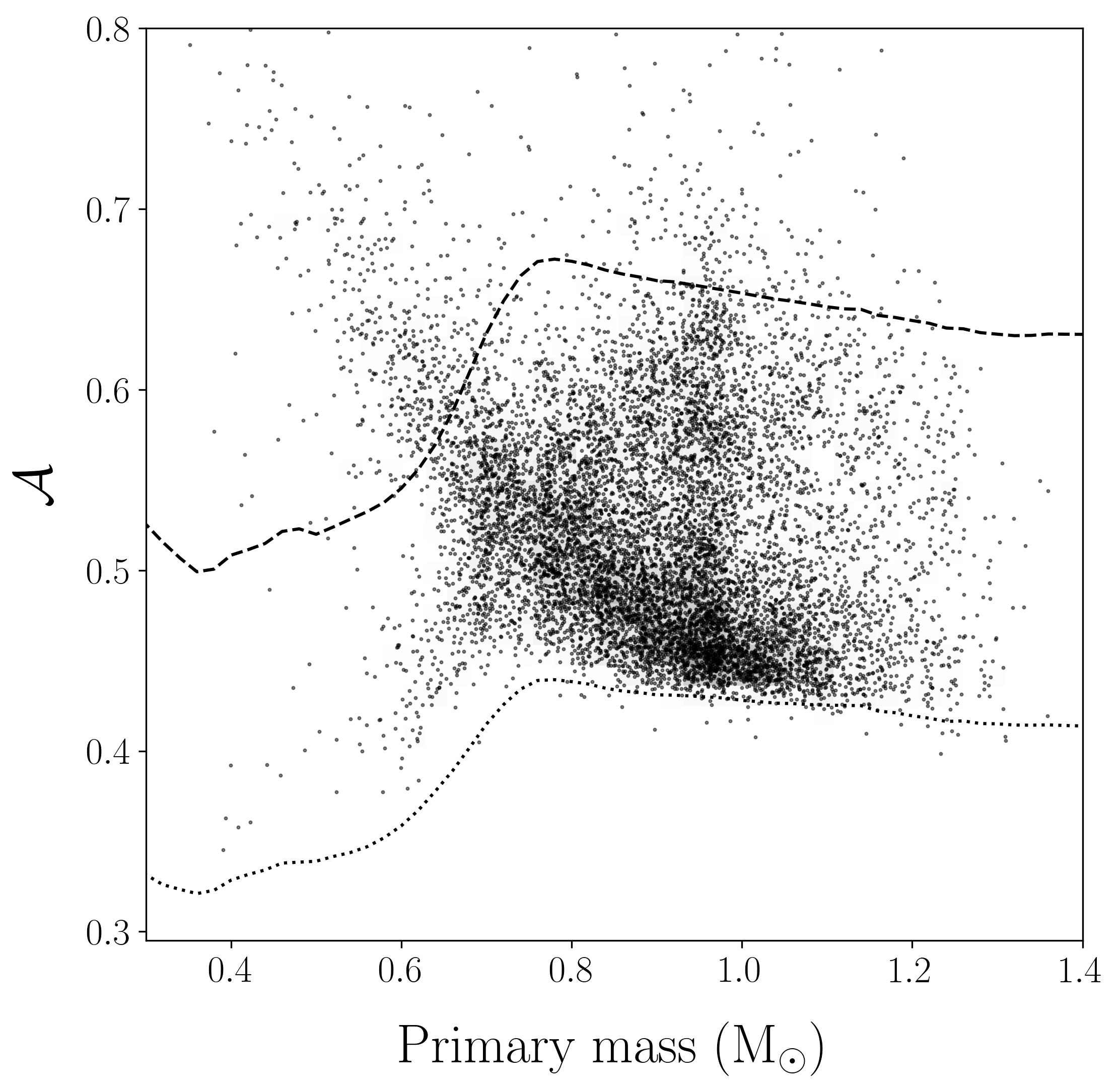
Figure 1: The astrometric mass-ratio function (AMRF) versus the primary mass of the $9\,786$ selected non-class-I systems. The dotted line separates between class-I and class-II regions, and the dashed line separates between class-II and -III.

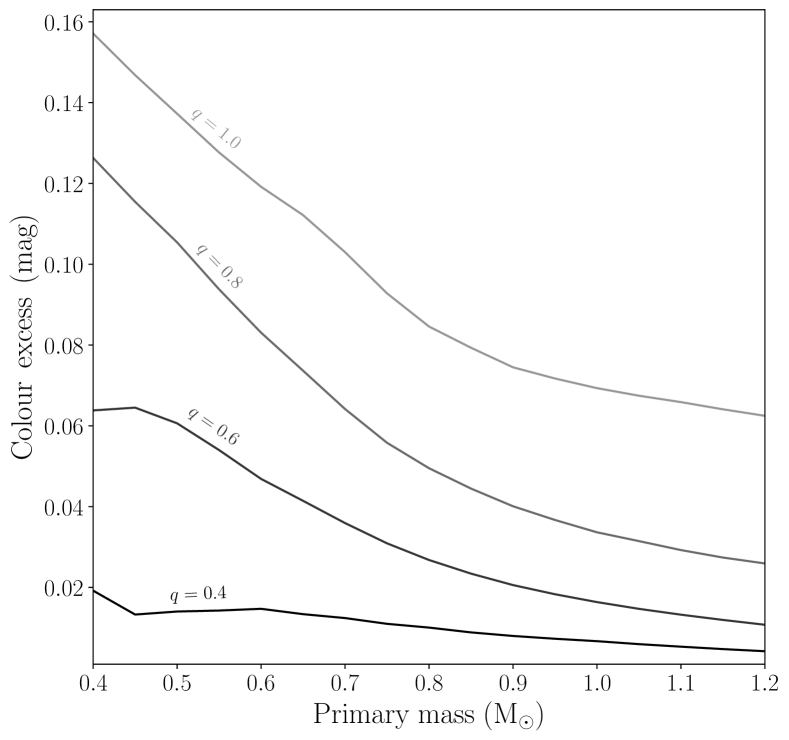
Figure 2: The $B-I$ colour excess induced by an unresolved binary system versus the mass of the astrometric primary star. Each line in the diagram corresponds to a different mass ratio, $q$, between the astrometric primary and secondary. The close binary is assumed to consist of two equal-mass MS stars.

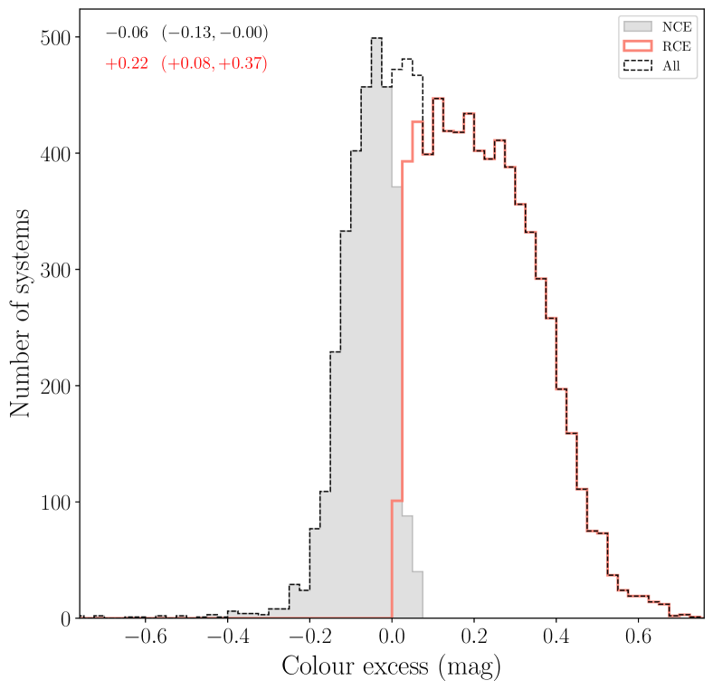
Figure 3: The estimated $B-I$ colour excess distribution of the red-colour excess (RCE) and no-colour excess (NCE) populations. The black dashed line shows the distribution of the full sample. The colour excess median and $36-84$th percentile range for the NCE (top row) and RCE (bottom row) populations appear in the top-left corner.

To identify astrometric binaries with WD companions, we compiled a sample of systems where the secondary component is less likely to be a single MS star. We then utilised the photometric measurements the Gaia mission provides to identify excess near-infrared emission to distinguish between hierarchical triple systems and MS+WD binaries. The data underlying this analysis are obtained from table 1 of Paper I and the following Gaia DR3 tables: gaia_source, nss_two_body_orbit, binary_masses, and synthetic_photometry_gspc.

2.1 Astrometric triage

The astrometric mass-ratio function (AMRF; Shahaf et al. 2019) is defined as

$$\mathcal{A}\equiv\frac{\alpha_{0}}{\varpi}\bigg{(}\frac{M_{1}}{\textrm{M}_{\odot}}\bigg{)}^{-1/3}\bigg{(}\frac{P}{\textrm{yr}}\bigg{)}^{-2/3}\,,$$ (1)

where $P$ is the orbital period, $M_{1}$ is the primary mass, $\varpi$ is the parallax, and $\alpha_{0}$ is the angular semimajor axis of the photocentric orbit.

Shahaf et al. (2019) showed that based on the AMRF value, one can assign each binary with an MS primary to one of three classes: class-I, where the companion is most likely a single MS star; class-II, where the companion cannot be a single MS star, but can still be a short-period binary of two MS stars; and, class-III, where the companion cannot be a single MS star or a close MS binary; therefore the faint astrometric secondary in such systems is probably a compact object.

Paper I used the AMRF approach to analyse a sample of $101\,380$ astrometric binaries reported in Gaia DR3. The selected binaries have MS primary stars, orbital periods shorter than $1\,000$ days, and orbital solutions that passed several quality criteria (see therein), estimating the probability of each system to be a class-II or class-III astrometric binary. These probabilities, denoted Pr II and Pr III, are provided in table 1 therein. Paper I used these classification probabilities to compile a short list of $177$ systems for which Pr III is close to unity. Assuming that Gaia’s orbital parameters are valid, their faint astrometric secondary components are likely to be compact objects. In this work, we take a different approach, excluding class-I systems instead of looking for class-III systems. Namely, we consider astrometric orbits for which the secondary is probably not a single MS star.

The class-I probability, Pr I, was not provided in Paper I but can be calculated using the other two classification probabilities,

$${\rm Pr\,I}=1-{\rm Pr\,II}-{\rm Pr\,III}+\frac{2}{N+1},$$ (2)

where $N=10^{5}$. We include in our sample only systems that satisfy the qualifying conditions outlined in Paper I (see section 3.1, therein) and have Pr I below $10$ per cent. This selection yielded $11\,190$ non-class-I systems.

Binaries with a primary mass larger than ${\sim}1.2$ ${\rm M}_{\odot}$ (within $1\sigma$), for which WD companions are unlikely to be classified as class-II or -III systems (see figure 2 of Paper I), were excluded from our sample. This selection criterion resulted in a $10\,080$ binaries. We then removed additional binaries for which the Gaia Synthetic Photometry Catalogue (GSPC; Gaia Collaboration et al., 2022b) did not provide estimates in the Johnson-Kron-Cousins bands (JKC; see below). Following this final step, we were left with a sample of $9\,786$ astrometric binaries, presented in Fig. 1.

2.2 Colour excess

2.2.1 Expected colour excess

We use Gaia’s spectrophotometric measurements to distinguish between hierarchical triples and MS+WD binaries and resolve this classification ambiguity. Fig. 3 shows the colour excess induced on the observed MS primary by an unresolved close-binary companion, using JKC’s $B$ and $I$ bands. We define the colour excess as the difference between the triple system’s and the primary star’s colours. Formally, this is given by

$$\begin{split}\Delta\left({B-I}\right)=&-2.5\log_{10}\left(10^{-0.4B_{1}}+10^{-0.4B_{2\text{a}}}+10^{-0.4B_{2\text{b}}}\right)\\ &+2.5\log_{10}\left(10^{-0.4I_{1}}+10^{-0.4I_{2\text{a}}}+10^{-0.4I_{2\text{b}}}\right)\\ &-\left(B_{1}-I_{1}\right)\,,\end{split}$$ (3)

where the subscript $1$ refers to the astrometric primary. The other two subscripts, 2a and 2b, refer to the two components of the astrometric secondary.

The estimates in Fig. 3 were calculated using PARSEC isochrones (Bressan et al., 2012; Chen et al., 2014, 2015; Tang et al., 2014). The close binary is assumed to comprise two equal-mass MS stars since this configuration yields the largest mass-luminosity ratio between the astrometric components. The figure illustrates that per-cent level photometric precision should be sufficient to identify the close-binary companions for systems with primaries less massive than ${\sim}1.2\,\mathrm{M}_{\odot}$.

2.2.2 Observed colour excess

Gaia DR3 catalogue provides flux-calibrated low-resolution spectrophotometric measurements in the wavelength range $330$–$1050$ nm. Based on these data, the Gaia Synthetic Photometry Catalogue (GSPC; Gaia Collaboration et al., 2022b) published synthetic photometric measurements with accuracy as low as ${\sim}10$ mmag. We compared the location of each source on the Gaia colour-magnitude diagram (CMD) to its theoretically expected position, assuming it is a single star, in search of excess infrared flux.

The system’s mass, age, metallicity, and extinction along the line of sight determine the theoretical CMD position. We used the estimates of Zhang et al. (2023b) for the metallicity. Systems flagged to have uncertain metallicity estimates by Zhang et al. (2023b) (their $\texttt{quality\_flags}~{}{\geq}~{}8$) were assigned with [M/H]$~{}{=}~{}0.00\pm 0.25$ dex. This choice is justified by the age-metallicity relation of stars in the solar neighbourhood (Rebassa-Mansergas et al., 2021). Systems with metallicity estimates laying outside of the PARSEC isochrones range ($-2\leq[\text{M/H}]\leq 0.6$) were assigned with the corresponding limiting values.

We used publicly available dust maps to account for reddening and extinction. Green et al. (2019) have created Bayestar19: a three-dimensional dust map that covers the northern hemisphere down to a declination of $-30$ deg. We used the dustmaps Python package to obtain the 16^th, 50^th, and 84^th percentiles of Bayestar19 extinction. These values were then multiplied by 0.884 to obtain the corresponding $E(B-V)$ values. For the southern systems, which were not included in Bayestar19, we used the three-dimensional dust map of Lallement et al. (2019). This map does not include error estimates. Considering systems included in both maps, the median difference between Bayestar19 and the Lallement et al. (2019) extinction is 0.02 mag. We therefore used this value as the uncertainty for the $E(B-V)$ values of the southern hemisphere systems. Finally, we converted the $E(B-V)$ values to $E(B-I)$ and $A_{V}$, using the relations

$$E(B-I)= (R_{B}-R_{I})\times E(B-V)\,\,\,\text{and}$$ (4)

$$A_{V}= R_{V}\times E(B-V)\,,$$

where the coefficients $R_{B}$, $R_{I}$ and $R_{V}$ were taken as $3.626$, $1.505$ and $3.1$, respectively (according to Munari & Carraro, 1996; Schlafly & Finkbeiner, 2011).

We estimated the colour excess using the Python package stam (Hallakoun & Maoz, 2021): Using PARSEC main-sequence isochrones, we generated a two-dimensional interpolant grid representing the relation between the $B-I$ colour index, the absolute $V$-band magnitude, and the metallicity. We limited the maximal mass of the isochrones to 1.17 $\mathrm{M}_{\odot}$ to avoid tracks that start to evolve off the MS, and assumed a fixed age of 2 Gyr. Stars do not significantly change their mass or appearance during their MS lifetime; therefore, this choice of isochrone age does not severely affect colour excess estimates. Our specific stellar age choice is consistent with the ages estimated for the more massive stars in our sample and justified by the observed evidence for a star formation burst in the Milky Way’s disc about 2 Gyr ago (Mor et al., 2019).

The observed colour excess is defined as

$$\Delta\left(B-I\right)=\left(B-I\right)_{\text{observed}}-\left(B-I\right)_{\text{expected}},$$ (5)

where $\left(B-I\right)_{\text{observed}}$ is the observed dereddened $B-I$ colour index, and the $\left(B-I\right)_{\text{expected}}$ is the theoretically expected $B-I$ value, assuming it is a single MS star. We calculated the theoretically expected values using the interpolant grid described above, with the system’s estimated metallicity and extinction-corrected absolute $V$-band magnitude as its independent variables.

We conduct a Monte-Carlo experiment to account for the uncertainties in the observed quantities and provide confidence intervals for the estimated colour excess. For each astrometric binary, we generated $10^{4}$ random realisations of its position on the metallicity-absolute magnitude grid. The absolute $V$-band magnitude of the system is not expected to change by more than $\sim 0.1$ mag by the presence of a WD companion (compared to a single MS star) for almost all our sample, except for those with primaries less massive than $\sim 0.3$ $\mathrm{M}_{\odot}$ and warm WD companions (see Section 4 and Fig. 11 below). We assumed that the metallicity and the absolute magnitude follow an uncorrelated bi-variate Gaussian distribution. The measurement uncertainties of the observed colour index and absolute magnitude were calculated following Hallakoun & Maoz (2021). For each instance, we calculated $\Delta\left(B-I\right)$ as described in equation (5). This sampled distribution’s mean and standard deviation provide our estimates for the colour excess expected value and uncertainty. We provide the colour-excess estimates for all the targets in our sample in Table 1.

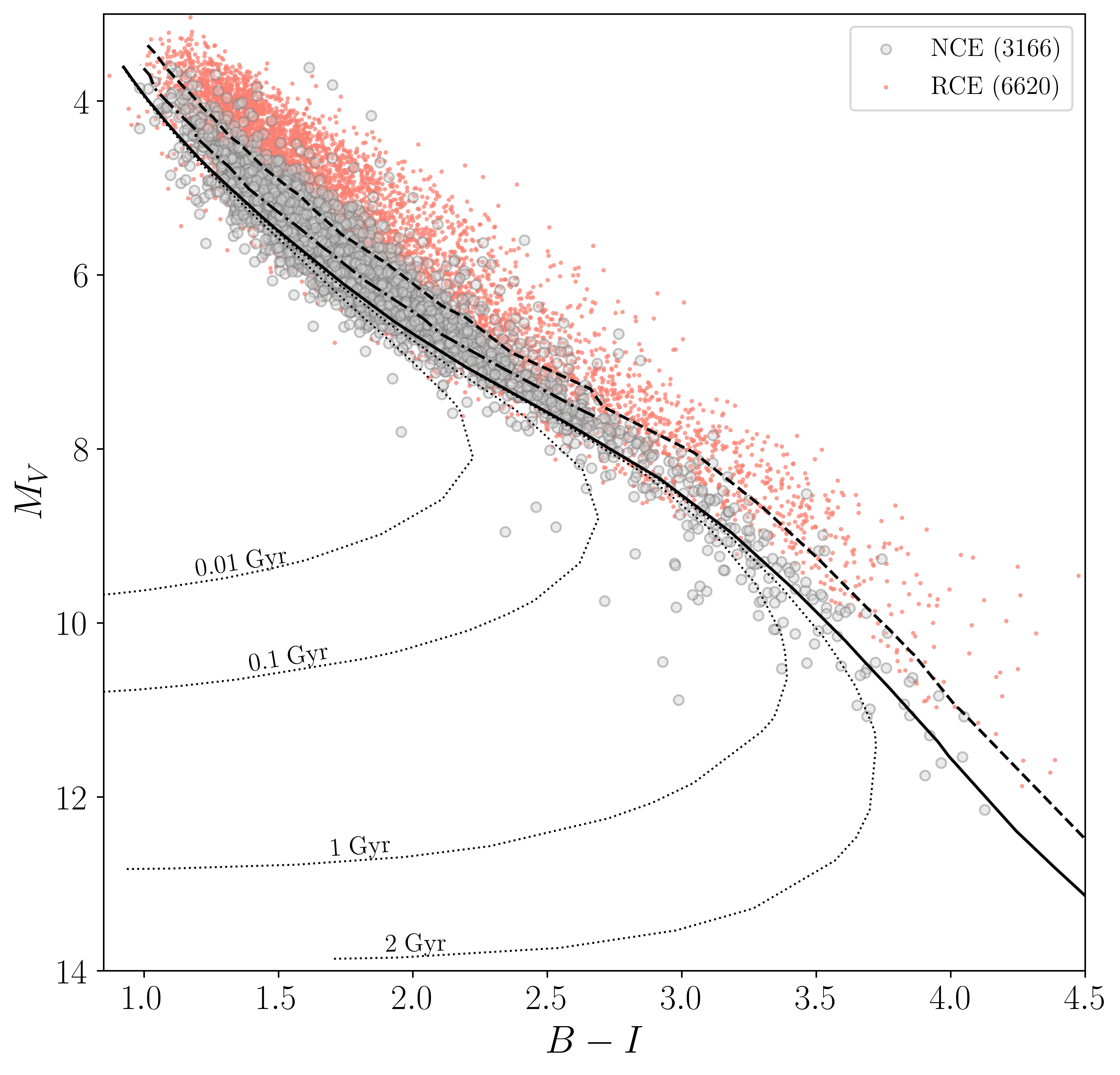
Figure 4: A colour-magnitude diagram for the $9\,786$ objects in our sample. The red-colour excess (RCE) and no-colour excess (NCE) populations are plotted as red and grey points, respectively. The number of objects in each population is given in the figure legend. A 2 Gyr isochrone of $[{\rm M}/{\rm H}]=-0.2$ is plotted as a solid black line. The dashed and dash-dotted black lines illustrate the position of binary and hierarchical triple systems, respectively, and the dotted lines represent the position of MS+WD binaries at different WD cooling ages (see text).

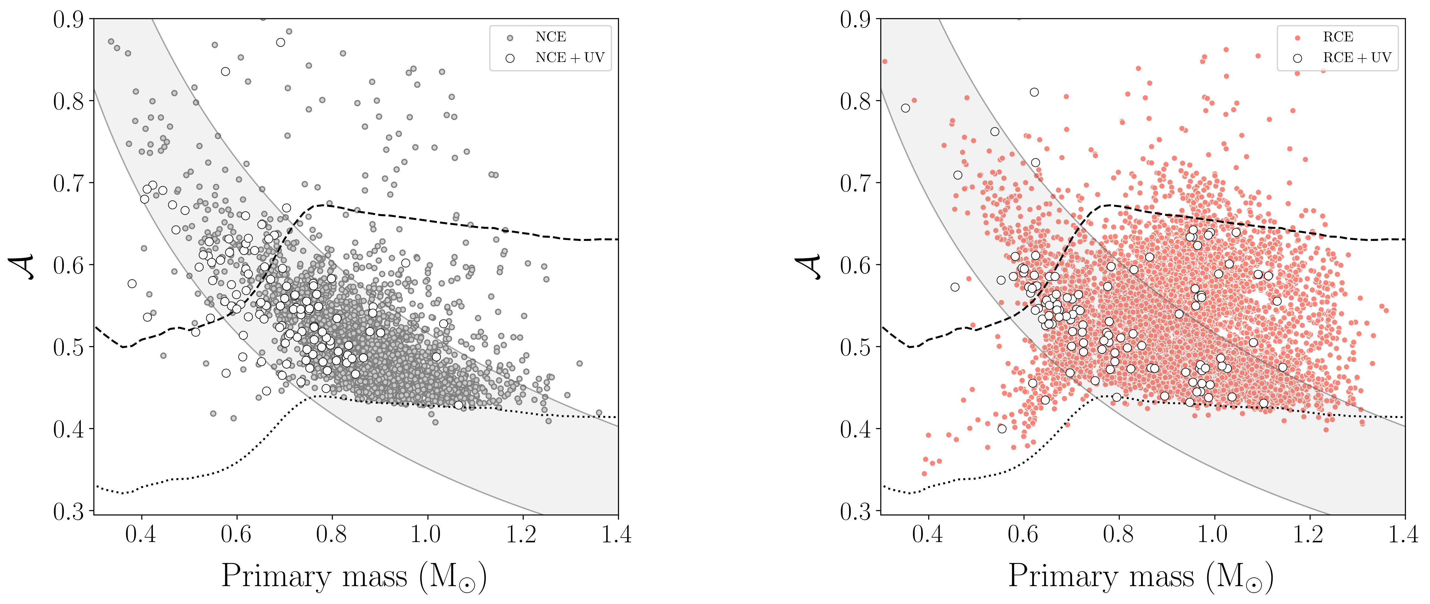
Figure 5: The AMRF versus the mass of the primary star, presented separately for the NCE (left panel) and the RCE (right panel) populations. The dotted line separates between class-I and class-II systems, and the dashed line separates class-II from -III. A grey strip highlights the expected location of systems with non-luminous companions in the mass range of $0.45{-}0.75\,\,\mathrm{M}_{\odot}$, where typical MS+WD binaries are expected to reside. The figure shows that, as a population, NCE systems tend to populate this area in parameter space, as opposed to the RCE sample. The white points depict systems in which excess emission in the near-UV band of GALEX was detected, as discussed in Section 3.2, which we ascribe to the contribution due to a WD companion. See Section 4 for a discussion of MS+WD contamination of the RCE sample.

2.3 Partitioning by colour excess

We define Pr(red) as the fraction of realisations where the dereddened observed colour index was larger than the expected colour excess. We have set the threshold above which a system is considered to have infrared excess to be the maximal Pr(red) value for which the measured colour excess is smaller than $10^{-2}$,

$${\rm Pr(red)}\geqslant 56~{}\text{per cent}.$$ (6)

This threshold ensures that we are sensitive to the expected colour excess from all triple systems in our sample (see Fig. 3). We provide the colour-excess probability for all the targets in our sample in Table 1.

Our non-class-I sample includes 6 620 systems with red colour excess (RCE). The remaining 3 166 targets do not exceed the above-mentioned threshold and will be referred to as no-colour-excess (NCE) systems. Fig. 3 shows the colour excess distribution of the entire population and the RCE and NCE subsamples.

Fig. 4 presents our sample, with red points indicating RCE systems and grey points representing NCE systems. A black line shows a 2 Gyr isochrone with a metallicity of [M/H] $=-0.2$, for demonstration (the colour-excess determination was performed individually for each system as described above). Using the same isochrone, we depict the positions of MS binaries, hierarchical triples, and MS+WD binaries. The black dashed line shows the location of binaries with a mass ratio of $0.8$; the dashed-dotted line represents triple systems with an equal-mass close binary as the faint astrometric companion, assuming a mass ratio of $0.8$ of the astrometric components; the dotted lines represent MS+WD binaries at various WD cooling ages, derived assuming a hydrogen-dominated WD with a mass of $0.6$ $\mathrm{M}_{\odot}$ (using the synthetic colours of Bergeron et al. 1995; Holberg & Bergeron 2006; Kowalski & Saumon 2006; Tremblay et al. 2011; Blouin et al. 2018; Bédard et al. 2020).

The colour excess estimate was obtained using synthetic photometry in the JKC system. Other systems, such as the SDSS system or Gaia’s $G_{\text{BP}}$ and $G_{\text{RP}}$ bands, can also be used. We found that the JKC’s $B-I$ colours are more sensitive to the colour excess than the broader Gaia $G_{\text{BP}}$ and $G_{\text{RP}}$ bands, and are available for almost all targets in our sample, as opposed to the SDSS synthetic photometry in the $u$ band.

3 A Census of white dwarfs

In the previous section, we identified a sample of astrometric binaries where the companion is unlikely to be a single MS star. Within this sample, we used the $B-I$ colour index to identify targets exhibiting red colour excess, allowing us to identify the contribution of light from close binary companions in hierarchical triple systems. Thus, we now have a sample (referred to as NCE) in which the secondaries are unlikely to be

1. single MS stars, or

2. close binaries of two MS stars.

The following section shows that the NCE sample is consistent with a predominantly MS+WD population.

3.1 Sample characteristics

Fig. 5 shows the relationship between the AMRF and the mass of the primary star for the NCE and RCE populations. The dotted line separates between class-I and -II systems, and the dashed line separates class-II from -III. The grey stripes represent the expected position of non-luminous companions in the mass range of $0.45-0.75~{}\mathrm{M}_{\odot}$. Notably, the two populations are differently distributed: The NCE sample is concentrated around the grey stripe, which corresponds to the expected mass range for WD companions; in contrast, the RCE sample is more spread out and populates a larger area on the $M_{1}-\mathcal{A}$ plane. The distribution of the NCE sample indicates that the population is mostly comprised of MS+WD binaries. However, the RCE sample is not a pure sample of hierarchical triples, as suggested by the RCE class-III binaries found on the grey stripe. These are likely MS+WD binaries that were found to have an apparent colour excess (see below).

Fig. 7 compares the distances, primary masses, $V$-band extinction, and Galactic latitudes of both populations. This figure shows that RCE systems are located at greater distances and closer to the Galactic plane than the NCE sample. The extinction histogram indicates that this may be due to our colour classification, as systems closer to the Galactic plane suffer from greater extinction and appear redder, suggesting that some of our extinction or metallicity estimates may be inaccurate. We further discuss this possibility in the following. An alternative explanation is that triple systems, which may be more luminous than MS+WD binaries, are observed at greater distances and show larger extinction values. The RCE primary-mass histogram in the top right panel of Fig. 7 shows an excess of ${\sim}1\,\mathrm{M}_{\odot}$ targets, accompanied by a deficiency of ${\sim}0.75\,\mathrm{M}_{\odot}$ primaries (which is also apparent in the right panel Fig. 5). These features do not appear in the NCE primary mass estimates. We do not have a concrete understanding regarding the cause of these features. We speculate they could be artefacts from the photometric mass estimation procedure of Gaia Collaboration et al. (2022a), caused by the light contribution from the astrometric secondary in hierarchical triple systems.

To test whether the differences between the populations are caused by vulnerabilities in the orbital fitting scheme, we checked for systematic differences in the number of measurements (visibility periods used; VPU), the goodness of fit (GoF), and the significance of the angular semi-major axis ($\alpha_{0}/\Delta\alpha_{0}$) and parallax ($\varpi/\Delta\varpi$). The corresponding histograms are plotted in Fig. 7. While the two populations follow similar trends in these four parameters, the NCE population seems to have slightly better significance and GoF values. This is expected, considering the larger distances and lower Galactic latitudes of the RCE sample.

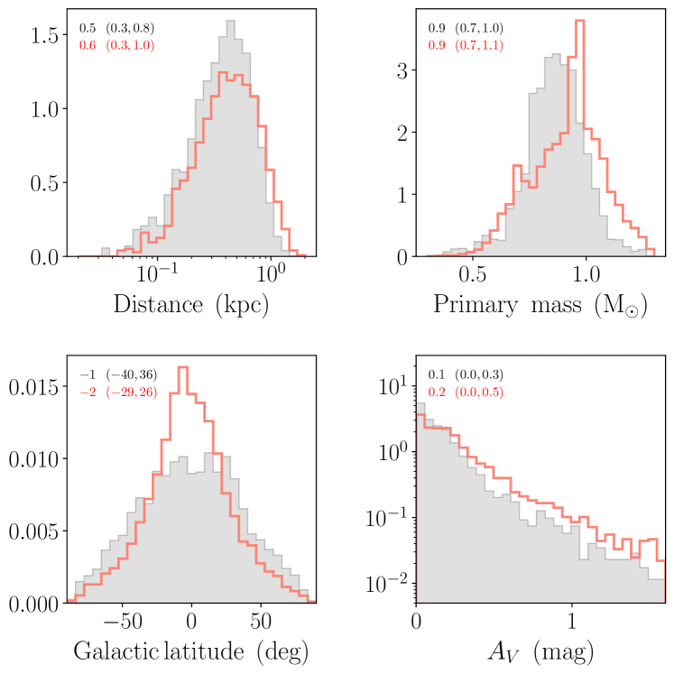
Figure 6: Distance, primary mass, $V$-band extinction, and Galactic latitude histograms (clockwise from top left) for the RCE sample (red line) and the NCE sample (grey bars). The median and the $36-84$ percentile range for each distribution are written on the top left corner of each panel, where the upper and lower rows describe the NCE and RCE samples, respectively.

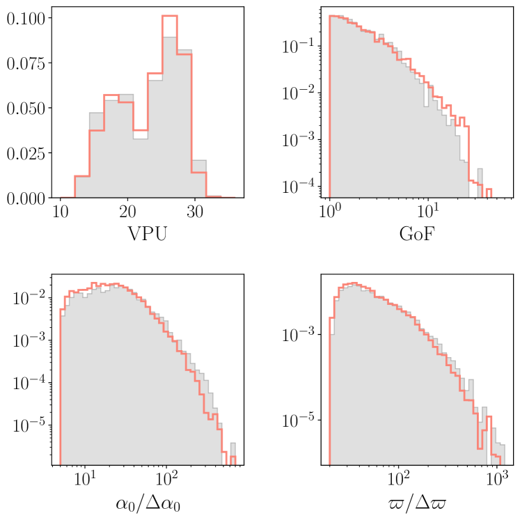
Figure 7: Properties of the selected sample. The two top panels show the number of visibility periods used (VPU; left) and the goodness of fit (GoF; right) reported in the Gaia catalogue. The significance of the angular semi-major axis (left) and parallax (right) are shown in the bottom panels. The colour coding is the same as in Fig. 7.

Fig. 8 presents the eccentricity versus the orbital period of the stars in the sample. Most of the eccentricities of the RCE sample (shown in the right panel) are below ${\sim}0.8$. This is probably an observational bias caused by the significant amount of time highly eccentric systems spend close to apastron, where the motion is not easily detected. Furthermore, most of the RCE binaries are found below the dotted line that indicates orbits that reach separations of ${\sim}100\,{\rm R}_{\odot}$ at periastron passage, assuming a total mass of $1\,\mathrm{M}_{\odot}$. On the other hand, the eccentricities of the NCE sample (shown in the left panel) are mostly below ${\sim}0.3$, as can be seen in the left panels of Fig. 9.

The secondary mass distribution of the NCE targets, shown in Fig. 9, peaks sharply around ${\sim}0.6\,\mathrm{M}_{\odot}$, consistent with them being MS+WD binaries. In contrast, the RCE sample displays a broader secondary mass distribution peaking at ${\sim}0.7\,\mathrm{M}_{\odot}$. However, even if we assume that the RCE sample is purely comprised of triple systems, inferring the secondary mass or mass-ratio distribution of hierarchical triple systems based on it is not straightforward. The secondary mass estimates assume negligible light contribution from the astrometric secondary (see table 1 in Paper I). This assumption is invalid for hierarchical triple systems, making these estimates merely lower limits of the secondary mass (Shahaf et al., 2019).

Fig. 9 also presents histograms of the orbital periods and the cosine of the inclination angle. Compared to the NCE population, the RCE population tends to have fewer systems with orbital periods below one year. One simple explanation is that RCE systems are found at greater distances, where relatively close separations are harder to detect. In addition, this difference might be due to the interaction between the present-day primary MS and the WD progenitor when it was a red giant. In terms of the inclination angle, the two populations exhibit similar distributions.

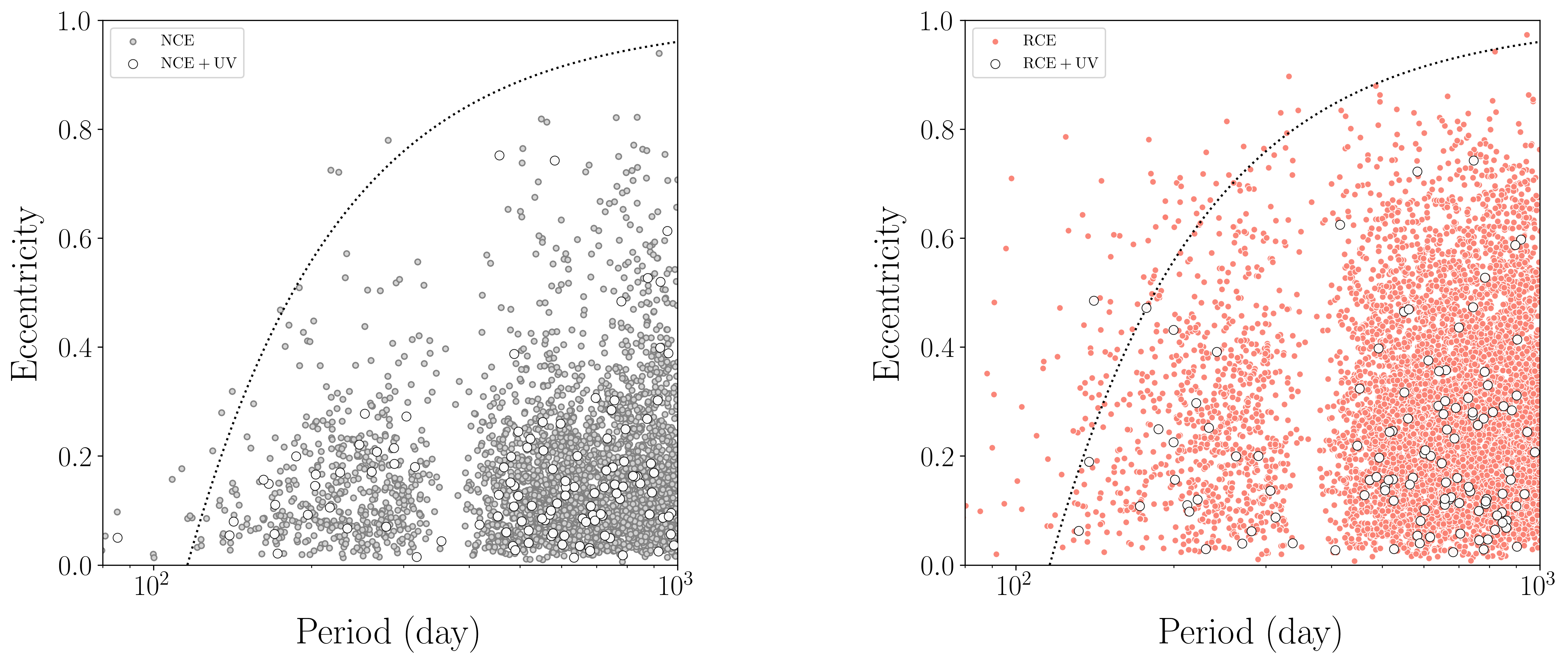
Figure 8: A period-eccentricity diagram for the NCE and RCE populations is plotted on the left and right panels, respectively. The gap corresponds to orbital periods of about one year. The dotted line represents an upper envelope that corresponds to periastron distance of ${\sim}100~{}{\rm R}_{\odot}$, assuming a total mass of $1~{}\mathrm{M}_{\odot}$. The white points depict systems in which excess emission was detected (see Figure 5 and Section 3.2).

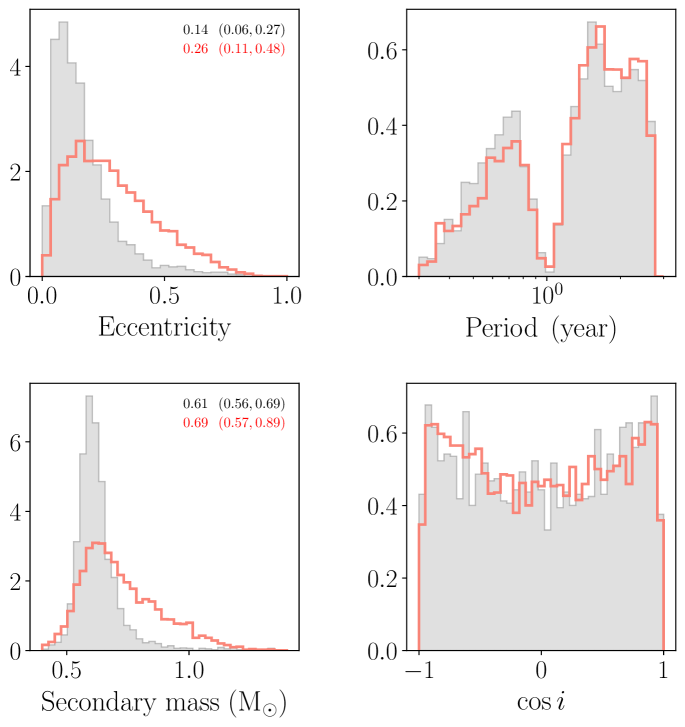
Figure 9: Histograms of the eccentricity, orbital period, cosine of the inclination angle, and secondary mass (clockwise from top left). The colour coding is the same as in Fig. 7. The two left panels, showing the eccentricity and secondary mass, also show the median and $36-84$ percentile range for the NCE (top line) and RCE (bottom line) populations.

3.2 UV excess

Newly formed WDs can significantly contribute to the binary system’s brightness in the visible bands (e.g., Fig. 4). This contribution becomes more pronounced in the UV, where MS primaries below ${\sim}1.2$ $\mathrm{M}_{\odot}$ are relatively faint. To identify these WD contributions, we searched the Galaxy Evolution Explorer (GALEX; Morrissey et al. 2007) database for UV counterparts to the NCE binaries in our sample. A similar analysis of the class-III binaries from Paper I was recently done by Ganguly et al. (2023).

We cross-matched the NCE targets in our sample with the GALEX all-sky imaging survey (AIS; Bianchi et al. 2011; Bianchi et al. 2017). The Gaia coordinates were propagated back to the coordinates at the AIS midpoint using the measured proper motion of each system. The fiducial search cone radius around each coordinate was $3$ arcsec (Bianchi & Shiao, 2020). This cone was enlarged to account for the proper motion of each system during the GALEX mission duration.

We have identified $3\,673$ matches between GALEX and Gaia targets, out of which $1\,436$ belong to the NCE population. Table 2 provides a list of the matched sources, including the Gaia and GALEX identifiers, apparent UV magnitude, and the angular separation between the matched sources. The median separation between the two positions of the matched sources is ${\sim}0.6$ arcsec. Only $7$ sources are separated by $3$ arcsec or more, with a maximal separation of ${\sim}3.6$ arcsec. There are $9$ targets for which we identified a second source within the search cone; we chose the closest one in these cases.

We use a simple single-valued relation to estimate the extinction in the GALEX near-UV (NUV) band. The relation is given by

$$A_{\rm NUV}\approx\frac{R_{\rm NUV}}{R_{\rm G}}A_{\rm G}\,\simeq 3.085\,A_{\rm G},$$ (7)

where $A_{\rm NUV}$ and $A_{\rm G}$ represent the extinction in the NUV and G bands, respectively. Their corresponding extinction coefficients, $R_{\rm NUV}$ and $R_{\rm G}$, were obtained from Zhang & Yuan (2023).

Fig. 10 presents the NUV absolute magnitudes of the NCE sample. The solid black line depicts the corresponding MS mass-luminosity relation obtained using our default isochrone (see above). The PARSEC NUV magnitudes are provided in the Vega photometric system; therefore, the derived relation was shifted by 1.699 mag to match the AB system of the AIS (Bianchi 2011). To illustrate the effect of extinction on the UV emission from the system, we added dashed and dotted black lines representing an extinction of $0.75$ and $1.5$ mag, respectively. These values roughly correspond to the 80^th and 95^th percentiles of the NCE sample.

Most points in Fig. 10 fall between the solid and dotted black lines, as expected. To illustrate the expected contribution of the WD, we plotted as dotted blue lines the expected absolute NUV magnitudes of $0.6~{}\mathrm{M}_{\odot}$ WDs with hydrogen-dominated photospheres at different cooling ages. For this purpose we used the tables6 of WD synthetic colours by Bergeron et al. (1995); Holberg & Bergeron (2006); Kowalski & Saumon (2006); Tremblay et al. (2011); Blouin et al. (2018); and Bédard et al. (2020). The diagram suggests that WDs with cooling ages below ${\sim}0.5$ Gyr should be easily detectable if their primary MS companions are of spectral types later than K.

Around 8 per cent of the NCE sample, 117 targets, show significant excess UV emission. As with the infrared colour excesses, we somewhat arbitrarily defined excess UV as a system brighter than expected MS single-star curve by more than $1\sigma$ (see Table 2). We accounted for the NUV magnitude, parallax, extinction and primary mass uncertainties. The RCE sample, for comparison, contains 118 binaries (${\sim}5$ per cent) showing NUV excess detected by the same criterion. However, nearly $40$ of these systems have primaries with masses of ${\sim}1$ $\mathrm{M}_{\odot}$, which is unlikely, given the young WD cooling ages implied. Considering the RCE primary mass distribution in Figure 7, it is likely that the expected NUV value of some of these systems is erroneous. The fraction of RCE systems with NUV excess is probably closer to ${\sim}3.5$ per cent.

As discussed in the following section, the colour-based sample segmentation aims to ensure that the NCE sample is less contaminated by triple systems, not vice versa. Therefore, we expect the RCE sample to contain triple systems and MS+WD binaries. Fig. 5 shows that the NUV-bright systems are localised around the WD grey stripe on the $\mathcal{A}{-}M_{1}$ diagram, both for the NCE and RCE samples, as expected. The higher occurrence of NUV-bright binaries in the NCE sample and the consistency of their secondary masses with the typical mass of a WD corroborates our classification scheme. The ratio between the two samples suggests that the contamination of the RCE sample can reach, at worst, about $60$ per cent. Still, a more detailed analysis of the spectral energy distribution of each system is required (e.g., Ganguly et al., 2023).

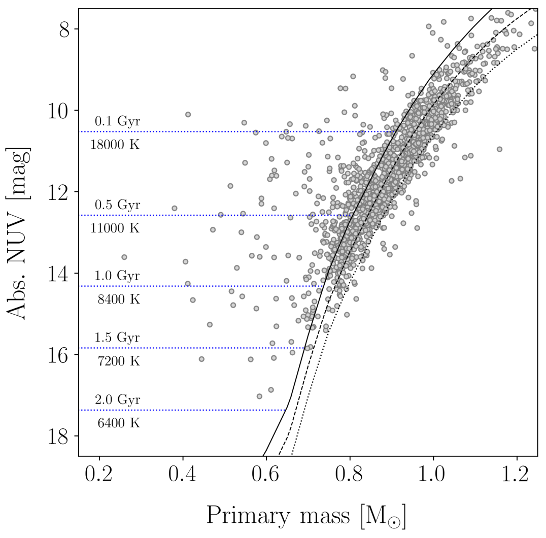
Figure 10: The GALEX NUV absolute magnitude versus the primary star’s mass. The grey circles represent the NCE binaries we have identified near-UV counterparts in GALEX (see text). The solid, dashed and dotted black lines represent the expected MS relation, based on a PARSEC isochrone of 2 Gyr, for extinction values of $0$, $0.75$ and $1.5$ mag, respectively. The horizontal lines show the expected NUV absolute magnitude of a $0.6\,\mathrm{M}_{\odot}$ WD at various cooling ages.

4 Biases and selection effects

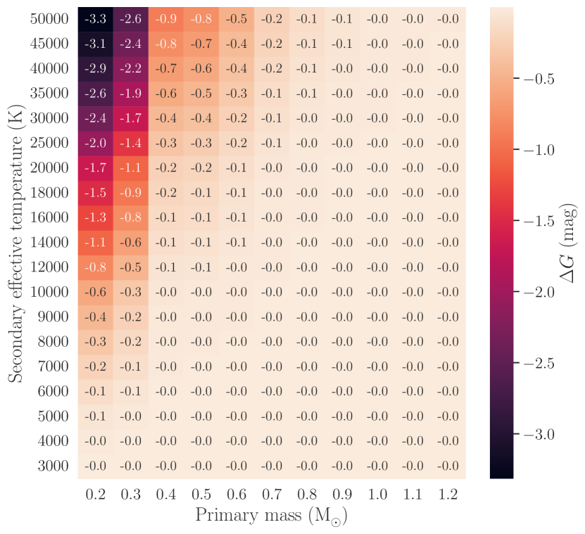
Figure 11: The expected photometric excess in the Gaia $G$ band of an MS+WD binary compared to the expected emission from the primary MS alone. This calculation assumes black-body spectra for both components and a 0.6 $\mathrm{M}_{\odot}$ hydrogen-dominated DA WD.

The first obvious selection effect in our NCE sample stems from the pre-selection of primary MS stars since low-mass MS stars will appear as photometric primaries in the Gaia $G$ band only if their WD companion is cool enough. However, this will affect only the smallest MS primaries, as demonstrated in Fig. 11, which shows the expected photometric excess in the Gaia $G$ band of an MS+WD binary compared to the expected emission from the primary MS alone, as a function of primary mass and WD effective temperature. From this figure it is clear that only binaries with a $\sim 0.3$ $\mathrm{M}_{\odot}$ MS star and a WD warmer than $\sim 16\,000$ K, or a $\sim 0.2$ $\mathrm{M}_{\odot}$ MS star and a WD warmer than $\sim 12\,000$ K, would be a priori excluded from our sample, since the WD would dominate the Gaia $G$ band. This explains the sparsity of systems with smaller primary masses (see Fig. 5). The expected photometric excess was calculated assuming black-body spectra for both components. The radius of the MS component was estimated using a 2 Gyr, [M/H] $=0$, PARSEC isochrone, while the WD radius was estimated using the WD_models Python package with the models of Bédard et al. (2020), assuming a 0.6 $\mathrm{M}_{\odot}$ hydrogen-dominated DA WD.

Our NCE sample, presumably primarily consisting of systems with WD companions, suggests that many MS+WD binaries exhibit a modest eccentricity of ${\sim}0.15$. This eccentricity might be linked to processes during the final stages of stellar or binary evolution (see Section 5.1.1 below). Thus, it is noteworthy that the eccentricity distribution of our sample is significantly biased. Fig. 12 presents the orbital eccentricity versus the system’s distance, indicating a tendency towards higher eccentricities with increasing distances. One explanation for this bias could be that the eccentricity is derived more accurately at closer distances; if the inference procedure is sensitive to correlated noise, this situation can result in biased eccentricity estimation (Lucy & Sweeney 1971; Bashi et al. 2022; also see, for example, a similar discussion by Hara et al. 2019 for the case of radial-velocity modelling of exoplanetary orbits). However, a comprehensive analysis to determine the origin of this bias requires a detailed study of Gaia’s selection function, which falls outside the scope of this study.

Another selection bias is related to the masses of the primary stars. The triage classification limits vary as a function of the primary star’s mass (see Fig. 5, for example). As a result, the WD mass distribution is biased since the minimal WD mass grows with the mass of the primary star, as Fig. 13 illustrates. One immediate consequence of this selection effect is a bias towards high WD masses and high mass ratios in the NCE sample. However, other biases may also stem from this selection effect. For example, since all the primary stars in our sample are on the MS, the correlation between the secondary and primary masses can be translated into a correlation between the WD’s mass and the binary system’s absolute magnitude. As a result, the maximal distance—and hence the orbital separation and eccentricity—of the detected systems might also be affected.

Finally, the assumption that the light contribution from the WD is negligible compared to that of the MS primary star is not necessarily accurate. Despite their compact nature, their contribution to the overall luminosity of the binary system may be non-negligible. If unaccounted for, this contribution may bias the WD mass estimates. The relative intensity of the WD compared to its MS companion depends on several factors, including the mass of the MS primary, the mass of the WD itself, and its cooling age. Since WDs cool with time over billions of years, younger WDs are brighter and bluer. In Fig. 14, we plot the minimal cooling age below which WDs contribute more than $5$ per cent of the system’s light in Gaia’s bandpass. WDs younger than this critical age can introduce bias more significant than ${\sim}10$ per cent to the mass estimation process. For systems with $\gtrsim 0.5$ $\mathrm{M}_{\odot}$ MS primaries and WDs with cooling ages older than ${\sim}0.5$ Gyr, the contribution of light from the WD cannot distort their mass estimates significantly.

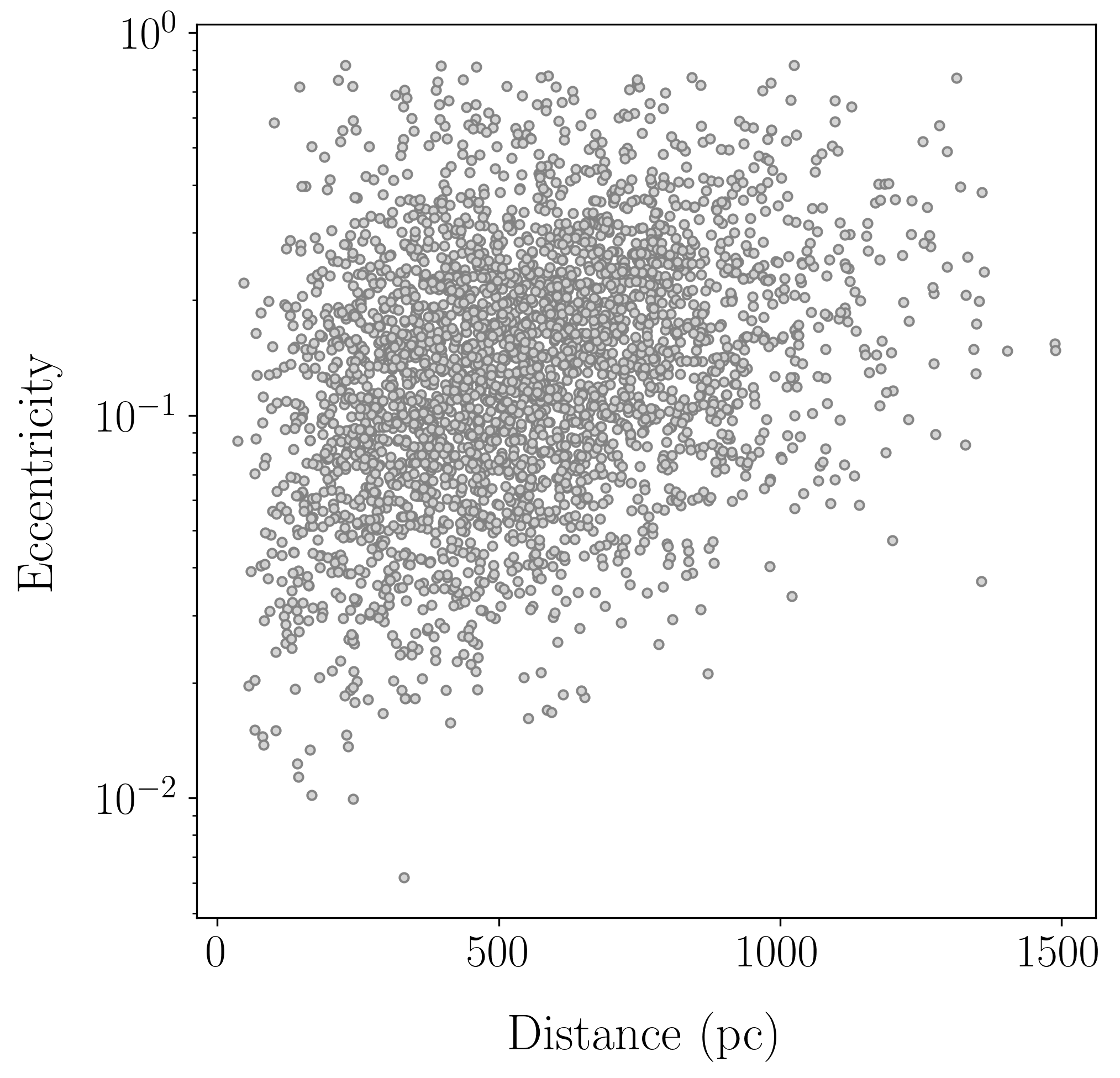
Figure 12: The orbital eccentricity versus the parallax distance for the systems in the NCE sample.

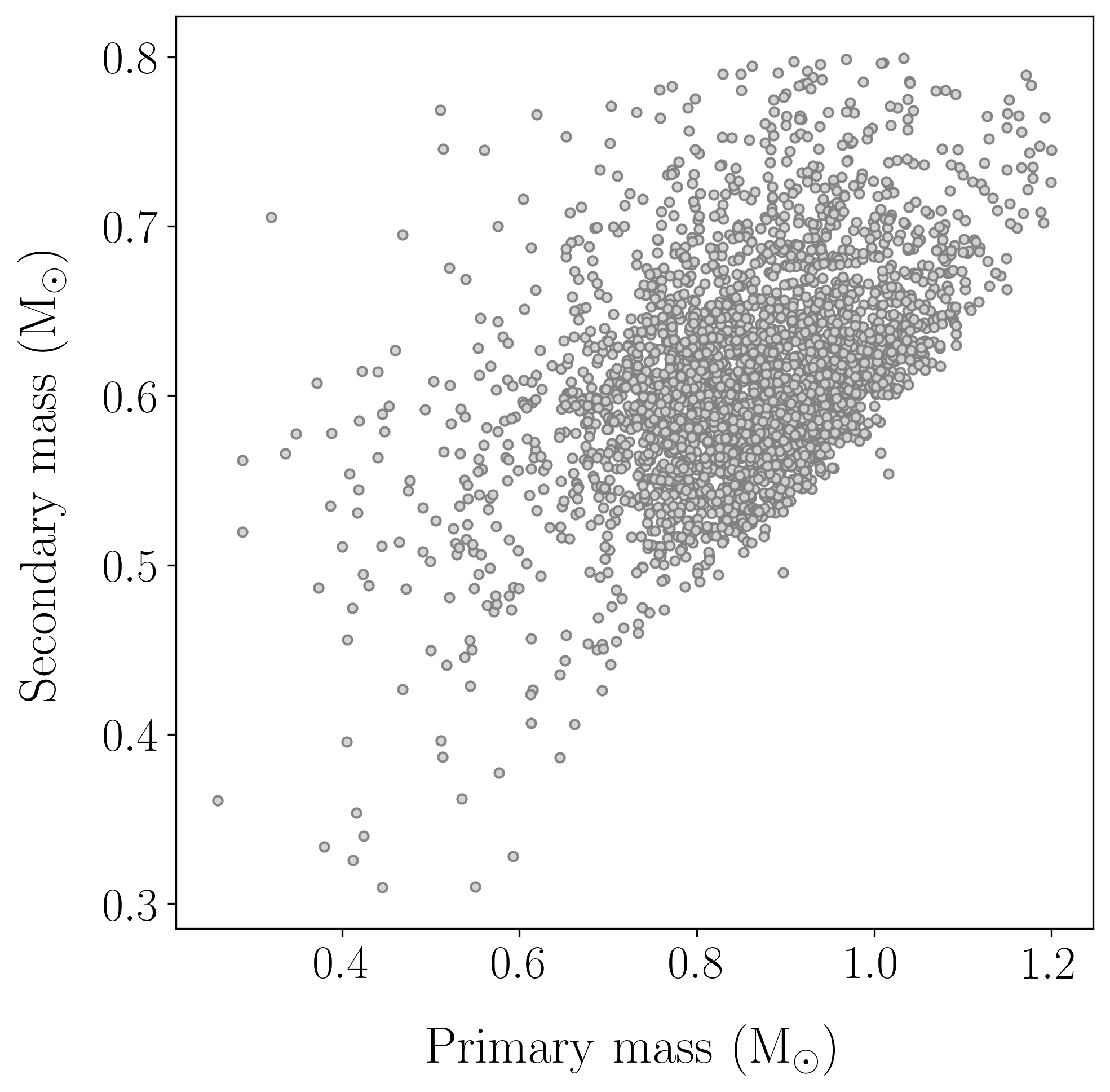
Figure 13: The secondary versus primary masses of the systems in the NCE sample. Systems with secondary masses larger than $0.8$ $\mathrm{M}_{\odot}$ are not included in this diagram.

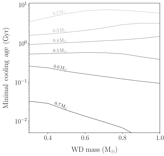
Figure 14: The minimal WD cooling age for which the $G$-band flux ratio between the WD and the MS drops below $5\%$ as a function of the WD mass. Each line represents a system with a different primary MS mass.

It is important to mention that the RCE sample does include some MS+WD binaries. For example, some of the RCE binaries are located above the class-III limit and within the region of the WD mass stripe of Fig. 5. Another indication of the WD contamination in the RCE sample is the NUV-bright systems. The position of these systems on the diagram is generally consistent with the WD stripe. Hence, these are likely misclassified MS+WD binaries identified as having excess infrared emission. This misclassification is probably the result of erroneous metallicity estimates for systems with primary masses smaller than $\sim 0.6$ $\mathrm{M}_{\odot}$ (see Fig. 15) that lead to an unreliable colour-excess assignment. This is consistent with fig. 18 of Zhang et al. (2023b), demonstrating the low fraction of reliable stellar parameter estimates for M dwarfs that were not included in the LAMOST training set used in that study. Luckily, almost the entire expected range of M-dwarf primaries with WD secondaries resides within class III on the AMRF plot (Fig. 5). Thus, all class-III systems with primary masses $\lesssim 0.6$ $\mathrm{M}_{\odot}$ are very likely to be MS+WD binaries, regardless of their assigned colour excess. Since there are very few class-II systems with M-dwarf primaries, the impact of this issue on our final MS+WD catalogue is small and can affect only systems with extremely low-mass WD companions. Better estimates of M-dwarf metallicities will enable more accurate classifications of these systems in the future.

Class-III systems with primaries more massive than $\sim 0.6$ $\mathrm{M}_{\odot}$ that are included in the RCE sample are more likely to have erroneous primary mass estimates (especially those with masses around $\sim 1$ $\mathrm{M}_{\odot}$, see discussion above). Alternatively, the assumption of 2 Gyr-old isochrones used for the colour-excess estimation (see Section 2.2) might be inaccurate for the systems with the most massive primaries, which could be either younger or already in the process of leaving the MS.

5 Summary and outlook

5.1 Astrophysical implications

The astrometric binaries presented here provide a uniquely large sample of nearly $3\,200$ probable MS+WD binaries with orbital separations of ${\sim}1$ au. These systems populate a region of parameter space largely unexplored by other observational techniques and have already yielded some insights into the WD population and binary evolution (Hallakoun et al., in preparation).

5.1.1 Binary evolution

On the one hand, the present orbits of many of the binaries are too small to allow for uninterrupted evolution of the WD progenitors through their red-giant phase; the eccentricity-period diagram displays some binaries with large eccentricities, such that the binary separation at the periastron is smaller than, say, $100~{}R_{\odot}$. On the other hand, their separation is likely too large to assume that they went through a common-envelope phase, as post-common envelope binaries with a WD and M-dwarf components have been found to exist only at the shortest periods (less than about two weeks, peaking at ${\sim}8$ hr; Nebot Gómez-Morán et al. (2011); Ashley et al. (2019); Kruckow et al. (2021); Lagos et al. (2022); Roulston et al. (2021), but see also Yamaguchi et al., in preparation, for some systems with periods of up to seven weeks). Therefore, some of these binaries, after the WD nature of the unseen companion is confirmed, might necessitate special binary evolutionary tracks (e.g. Perets & Fabrycky, 2009).

Stable mass transfer is a known mechanism to form long-period binaries with WD components. In fact, theory predicts a relation between the period and the WD mass for systems that have evolved this way (Rappaport et al., 1995; Chen et al., 2013). For WD masses between $0.45-0.5\,\mathrm{M}_{\odot}$ and donor stars on the Red Giant Branch (RGB), Chen et al. (2013) predicts periods between $600-935$ days and $275-428$ days at metallicities of $z=0.01$ and $z=0.0001$, which are in good agreement with the periods of our sample. However, most of our WD masses are above $0.55\,\mathrm{M}_{\odot}$, so their direct progenitors cannot be RGB stars but must have already been on the Asymptotic Giant Branch (AGB) at the onset of the mass transfer. While mass transfer with an AGB donor is typically expected to lead to a common-envelope phase (e.g. Hjellming & Webbink, 1987; Hurley et al., 2002, but see Mohamed & Podsiadlowski 2007), our systems imply stable mass transfer is possible, likely aided by mass loss through non-conservative mass transfer (Soberman et al., 1997). In addition, the eccentricities of our systems cannot easily be explained by stable mass transfer alone since, in classical binary evolution theory, tides would circularise the orbit before the onset of the mass transfer. Possible eccentricity pumping mechanisms are enhanced wind mass loss at periastron (Van Winckel et al., 1995; Bonačić Marinović et al., 2008), Roche-lobe overflow at periastron (Soker, 2000; Vos et al., 2015), formation of a circumbinary disc (Waelkens et al., 1996; Dermine et al., 2013; Vos et al., 2015), and WD natal kicks (Izzard et al., 2010).

If some of these binaries underwent mild mass-transfer interaction, we might find evidence for heavy s-process element pollution in the luminous MS star atmosphere. Very few known Barium stars are in our sample, and more generally in the Gaia non-single star catalogue. Interestingly, the period-eccentricity distribution in the left panel of Fig. 8 resembles that seen in Barium stars at a similar range of orbital periods (e.g., Jorissen et al. 2016, 2019; Escorza & De Rosa 2023). The orbital elements and amount of enrichment may uncover the properties of the WD progenitors and the underlying mass-transfer process. Sayeed et al. (2023), for example, recently proposed binary evolution as a possible formation pathway of fast-rotating chemically enriched red giants. Studying the element abundances of the systems in our catalogue may uncover the properties and significance of these mechanisms in a different range of separations and binary evolution stages.

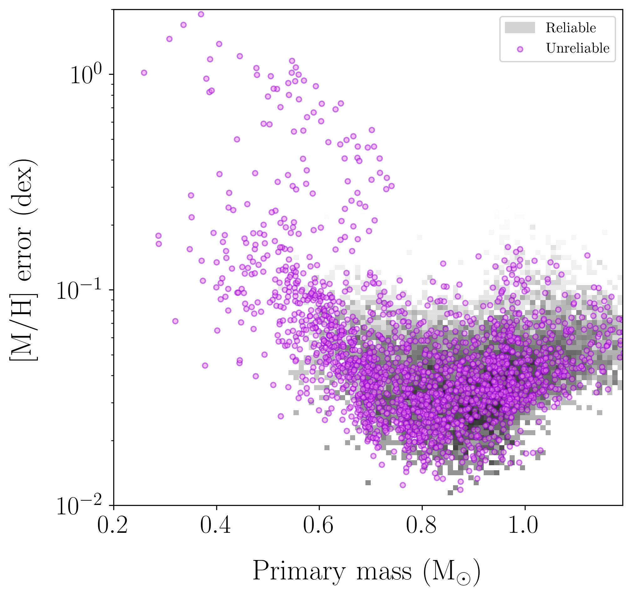
Figure 15: The metallicity error as a function of primary mass of all non-class-I systems. Reliable [M/H] estimates ($\texttt{quality\_flags}<8$ in Zhang et al. 2023b) are shown in the greyscale two-dimensional histogram. Unreliable [M/H] estimates ($\texttt{quality\_flags}\geq 8$) are plotted as violet circles. These systems were assigned a metallicity of $0\pm 0.25$ dex in our analysis (see Section 2.2).

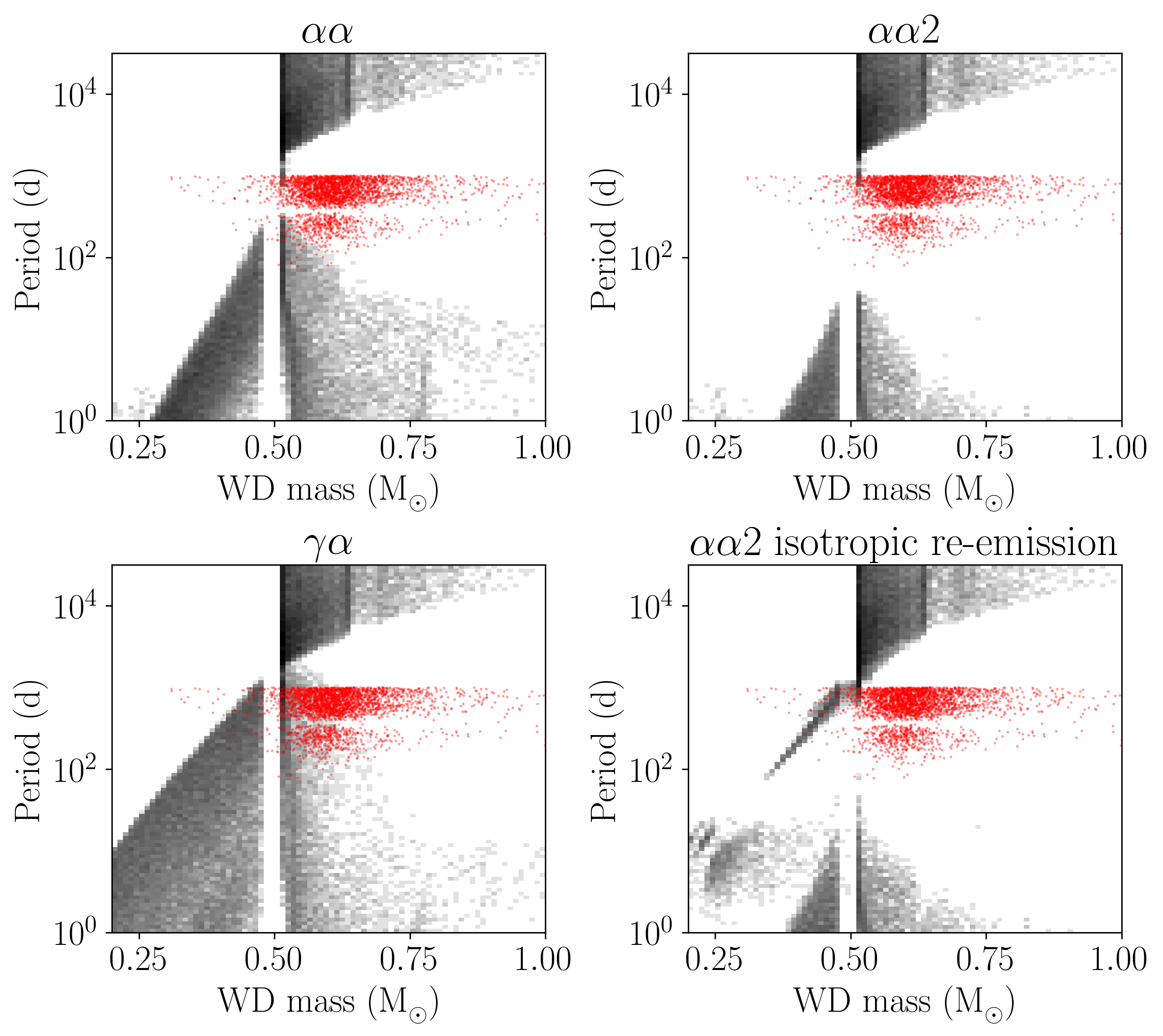
Figure 16: A comparison to a synthetic population of MS+WD binaries with $M_{\textrm{MS}}\leq 1.2$ $\mathrm{M}_{\odot}$. Each panel shows the predicted period vs. WD mass distribution (coloured in logarithmic scale) assuming a different SeBa model (see text for details; clockwise from top left): standard $\alpha\alpha$ model, standard $\alpha\alpha$ model with severe shrinkage in the common-envelope phase, the same as the previous but with isotropic re-emission, and the standard $\gamma\alpha$ model. The Gaia NCE sample is plotted as red dots.

Fig. 16 compares the period-mass distribution of the observed NCE sample with the predicted distribution of various binary population synthesis (BPS) models. The synthetic populations shown here were generated using the SeBa BPS code (Portegies Zwart & Verbunt, 1996; Nelemans et al., 2001; Toonen et al., 2012). The models differ in their treatment of the common-envelope phase. The process is parameterised using scalar factors governing the efficiency with which energy or angular momentum transfer unbind the envelope. These parameters are often denoted “$\alpha$” (Paczynski, 1976; Webbink, 1984; Livio & Soker, 1988) and “$\gamma$” (Nelemans et al., 2000; Nelemans & Tout, 2005; van der Sluys et al., 2006), respectively. The expulsion of the envelope shrinks the orbit of the binary in a process that can lead to the formation of a close double-WD system. These systems presumably experienced at least two phases of mass transfer, of which at least one occurred during a common-envelope phase.

The BPS samples used here rely on two model families, $\alpha\alpha$ and $\gamma\alpha$ (Toonen et al., 2012), defined based on the formalism used for each common-envelope phase. The $\alpha\alpha$ prescription, which is the standard model in most BPS codes (i.e. $\alpha\lambda=2$, where $\lambda$ is a parameter that depends on the structure of the donor star), has two additional variants: The $\alpha\alpha 2$ model, capable of producing a more significant orbital shrinkage during the common-envelope phase (i.e. $\alpha\lambda=0.25$), was developed to match known populations of close MS+WD binaries (Toonen & Nelemans, 2013; Zorotovic et al., 2010; Camacho et al., 2014; Scherbak & Fuller, 2023); The $\alpha\alpha 2$ model with isotropic re-emission, in which mass is allowed to leave the system with the specific angular momentum of the accretor (instead of 2.5 times that of the orbit), is also capable of producing wider orbits. The resulting period versus WD mass distributions of all four prescriptions are presented in Fig. 16, derived during the MS+WD evolutionary stage of the synthetic population.

The observed NCE population is plotted as red dots in Fig. 16. Although this population is affected by the selection criteria and observational biases, it is useful to consider whether current BPS codes are at all capable of producing it. We note that we only consider simulated MS+WD systems where the mass of the MS star is smaller than 1.2 $\mathrm{M}_{\odot}$, to reflect the selection in our observed sample. The $\alpha\alpha$ model and its variants have gaps around orbital periods of a few hundred days, where our observed NCE sample resides. Therefore, while some $\alpha\alpha$ variants might further improve by adjusting their parameters, this prescription seems less suitable for describing the observed NCE population. In contrast, the $\gamma\alpha$ model, which employs the $\gamma$ formalism for the first mass transfer event, succeeds in generating some MS+WD systems in part of the observed parameter range. This model was developed in order to match known populations of close double-WD binaries (Nelemans et al., 2000; Nelemans & Tout, 2005; van der Sluys et al., 2006). We note, however, that all these models fail to reproduce MS+WD binaries with eccentricities larger than zero, in contrast with our observed sample.

If indeed the NCE sample represents a homogeneous MS+WD population, Fig. 16 suggests that some BPS prescriptions do not fully describe the binary population at the ${\sim}1$ au separation range. This unprecedentedly large sample of MS+WD systems with intermediate orbital separations should help constrain and adjust these models to better fit the observations.

5.1.2 WD initial to final mass relation

Fig. 10 suggests we can estimate the cooling ages of many WDs in our sample based on their UV excess. Since the WD masses were dynamically measured, estimating the binary’s age would allow us to derive an empirical initial-to-final mass relation (IFMR) for these WDs. In most cases, these relations are obtained for single WDs in clusters (e.g. Cummings et al., 2018).

This sample allows for empirical estimation of the IFMR in binary systems with orbital separations potentially small enough for inducing interaction during the late stages of the WD progenitor’s evolution. However, determining the age of MS stars presents a challenge. Techniques like Gyrochronology (Bouma et al., 2023) or abundance analysis may be helpful, yet their reliability, considering the configuration and evolutionary history of the binaries in our sample, is unclear (Silva-Beyer et al. 2023; Gruner et al. 2023). An alternative approach would be associating MS+WD binaries with open clusters. Even though the numbers are relatively small, these systems provide a reliable age estimate for the WD and the binary as a whole.

5.2 Caveats and limitations

As in the first paper, we rely heavily on the validity of the orbital solution provided by Gaia. For example, the follow-up campaign for the relatively small class-III sample in Paper I required dozens of observations over many months. Scaling up an initiated spectroscopic campaign to dynamically validate the orbits of thousands of systems might be impractical. Alternative approaches, such as non-dynamical validation via detailed modelling of the spectral energy distribution or archival velocity measurements, may be useful.

The infrared-excess classification scheme aims to identify hierarchal triples, not MS+WD binaries. As a result, the RCE sample is not purely comprised of triple systems. The classification probabilities and estimated B-I colour excess values are provided in Table 1, to enable other studies of this population that may require different confidence levels. Furthermore, as discussed in Section 4, the samples presented in this work are biased; astrophysical conclusions drawn based on them must take these biases into account.

Astrometric binaries with an MS primary more massive than ${\sim}1.2\mathrm{M}_{\odot}$ will appear as class-I binaries even if their companion is a WD. This is not a trivial limitation, as detecting A-type stars with WD companions is beyond the reach of the triage method. A complementary approach, using interferometric measurements, was recently presented in a series of publications by Waisberg et al. (2023m, n). Their analysis enabled the detection and characterisation of WD companions to A-type MS primaries at orbital periods on the order of a few tens of years (also see Waisberg et al. 2023a, b, c, d, e, f, g, h, i, j, k, l).

An astrophysical scenario not considered in this work is a triple system in which the secondary companion is a binary comprised of a close binary of a WD and a low-mass MS star. While the occurrence and evolutionary path leading to such systems in this separation range is unclear, empirical constraints on their occurrence might be of interest. In the context of this work, such a system could, in principle, demonstrate excess emission both in short and long wavelengths.

5.3 Prospects for future work

The samples presented in this work offer an opportunity to probe the biases and selection effects in the Gaia catalogue. The NCE sample represents a homogeneous population of binary systems: The light contribution of both components in these binaries can be reliably constrained, their orbits are expected to be fairly circularised, and they are found at various Galactic latitudes. One can, therefore, use it to derive Gaia’s selection function for binary orbits (e.g., Rix et al., 2021; Cantat-Gaudin et al., 2023; Castro-Ginard et al., 2023).

For some science cases, validation of the orbits and classification validity may be required. Medium-resolution broadband spectroscopy offers a straightforward path to determine the nature of systems in our NCE sample. The spectra will allow us to characterise the primary star, leading to better constraints on its mass and metallicity. Excess emission at wavelengths $\leq 450$ nm ($\geq 750$ nm) might reveal the presence of a WD (late-type M-dwarf) companion. Fig. 17 shows the signal-to-noise ratio (SNR) required to detect a WD at a given effective temperature (i.e. cooling age) versus wavelength assuming an MS primary of 1 $\mathrm{M}_{\odot}$. The component radii were estimated similarly to those of Fig. 11 (see Section 4).

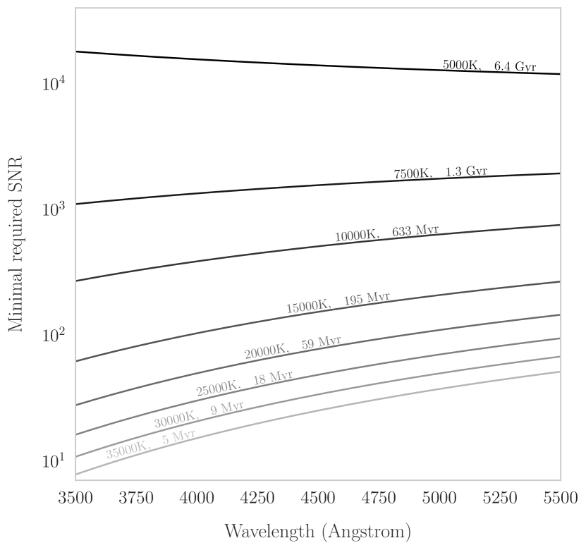
Figure 17: Minimal SNR required to detect a 0.6 $\mathrm{M}_{\odot}$ WD companion to a 1 $\mathrm{M}_{\odot}$ MS star. Each line corresponds to a different WD effective temperature (or cooling age). This calculation assumes black-body spectra for both components. The calculation is performed at a spectral resolution of $1\mbox{\AA}$.

As the median magnitude of a target in our sample is relatively bright ($G=14.33$) and the measurements are not time-critical, a flexible program for telescopes operating in queue mode will be an effective follow-up strategy. The upcoming Son of X-Shooter (SoXS) spectrograph, expected to see first light in early 2024 on the European Southern Observatory (ESO) $3.6\,$m New Technology Telescope (NTT), is our case study for such a program. The spectrograph offers a resolution of $R{\sim}4\,000$ from $0.35$ to $2.1\upmu$m in a single exposure (Schipani et al., 2020; Rubin et al., 2020). Using the SoXS Exposure Time Calculator, we find that a ${\sim}150$ sec exposure is sufficient to achieve an SNR of $10$ at the short wavelength range of the spectrograph. At ${\sim}1\,\upmu$m a $25$ sec exposure is required to reach the same SNR, similar to the exposure time required at ${\sim}0.4\,\upmu$m.

Some studies, such as determining the WD IFMR, may require additional spaceborne UV measurements. For example, detailed studies of individual systems containing young WDs can utilise the Cosmic Origins Spectrograph (COS; Osterman et al. 2011) on board the Hubble Space Telescope (HST) to determine their effective temperature, surface gravity and composition. On the other hand, the Wide-Field Camera 3 (WFC3; Teplitz et al. 2013) on the HST can be used to determine open clusters and WD cooling ages efficiently.

The samples in this work can provide insights into binary and stellar evolution and identify biases in the astrometric binary population. With the forthcoming fourth data release of Gaia, our analysis can be extended to longer orbital periods. This will clarify the processes at the onset of mass transfer and their impact on binary evolution and the Galatic WD population.

Data Availability

All data underlying this research are publicly available.

Appendix A Tables

Source ID	RA	Dec	$\varpi$	$M_{1}$	$[{\rm Fe/H}]$	abs. V	B–I	$A_{\rm V}$	CE	Pr (red)
	(Deg)	(Deg)	(mas)	(${\rm M}_{\odot}$)	(dex)	(mag)	(mag)	(mag)	(mag)	$(\%)$
3334754343120640	48.893	5.471	3.01	0.6	-0.945(61)	8.227(55)	2.779(11)	0.493(96)	0.25(21)	89.43
10378500708692608	49.532	7.405	6.73	0.7	-0.543(37)	7.888(76)	3.082(10)	0.027(29)	0.37(25)	96.56
13499150931192576	53.145	11.734	1.91	0.8	-0.383(77)	6.79(12)	2.407(12)	0.740(20)	0.25(19)	90.83
13966000991651456	47.822	8.848	5.39	0.7	-0.480(35)	7.500(59)	2.7897(78)	0.836(90)	0.36(19)	97.17
14998957806126592	45.486	9.544	2.83	1.0	-0.001(30)	5.283(65)	1.6924(43)	0.466(37)	0.02(12)	57.57
22172240385273088	42.461	10.675	1.77	0.9	0.346(31)	5.40(16)	1.8424(48)	0.411(27)	0.00(15)	50.97
28923104340937600	45.321	13.035	3.82	1.0	-0.046(39)	4.45(24)	1.4547(47)	0.384(20)	0.08(15)	72.67
34377639791849984	46.833	16.147	4.02	1.2	-0.824(91)	3.62(15)	1.2764(74)	0.356(47)	0.40(15)	99.67
37150234457357312	57.733	13.161	0.99	1.1	-0.402(82)	4.646(98)	1.6268(53)	0.630(47)	0.23(13)	95.79
38662372182863104	58.068	13.413	1.00	1.0	-0.255(86)	4.593(96)	1.7871(52)	0.658(75)	0.34(15)	98.92

Table 1: The cleaned sampled of non-class-I objects in out sample. The Source ID, RA, Dec, and parallax were obtained from the nss_two_body_orbit table, and the primary mass was obtained from binary_masses table (Gaia Collaboration et al. 2022a). The absolute $V$-band magnitude and the $B$-$I$ colours were calculated using the synthetic_photometry_gspc table (Gaia Collaboration et al. 2022b), and appear in the table without extinction and reddening correction. The metallicity values used were selected as described in Section 2. CE and Pr (red) are the colour excess and the red excess probability, respectively. The full table is available in the supplemental information accompanying this publication.

Source ID	GALEX ID	sep	NUV	FUV	Excess
		(mas)	(mag)	(mag)	(mag)
14998957806126592	6377073069995853037	0.94	19.080(60)		0.6(1.1)
22172240385273088	6377213859023816129	0.68	21.53(33)		1.4(1.1)
28923104340937600	6377073044226049205	1.25	17.063(28)		0.33(87)
34377639791849984	6377073031343243419	0.74	14.787(11)	20.18(25)	-0.18(60)
41408333753757056	6377073115093010630	1.98	22.46(46)		-6.5(1.1)	*
41954481793705984	6377073095765656506	2.27	20.98(24)		-5.5(1.8)	*
43892267960691840	6376967475003655762	0.4	18.490(60)		-0.2(1.3)
44082998867371776	6376967470708689546	0.6	21.71(38)		0.8(1.1)
45281840202132224	6376967527617005236	0.32	18.355(32)		-0.1(1.1)
50144812630106240	6376861957322965342	0.7	20.14(14)	19.81(16)	-4.7(1.8)	*

Table 2: UV data of 3 672 binaries from our sample with an identified counterpart in GALEX. The first three columns present the Gaia and GALEX IDs and the angular separation in mili-arcsec between the two sources. The fourth and fifth columns provide the GALEX apparent magnitudes without extinction correction. The sixth column provides the calculated excess absolute NUV magnitude (see text). An asterisk is used to indicate systems that were identified with excess UV emission. The full table is available in the supplemental information accompanying this publication.

References

- Ashley et al. (2019) Ashley R. P., Farihi J., Marsh T. R., Wilson D. J., Gänsicke B. T., 2019, MNRAS, 484, 5362
- Astropy Collaboration et al. (2013) Astropy Collaboration et al., 2013, A&A, 558, A33
- Astropy Collaboration et al. (2018) Astropy Collaboration et al., 2018, AJ, 156, 123
- Bashi et al. (2022) Bashi D., Shahaf S., Mazeh T., Faigler S., Dong S., El-Badry K., Rix H. W., Jorissen A., 2022, MNRAS, 517, 3888
- Bédard et al. (2020) Bédard A., Bergeron P., Brassard P., Fontaine G., 2020, ApJ, 901, 93
- Bergeron et al. (1995) Bergeron P., Wesemael F., Beauchamp A., 1995, PASP, 107, 1047
- Bessel (1844) Bessel F. W., 1844, MNRAS, 6, 136
- Bianchi (2011) Bianchi L., 2011, Ap&SS, 335, 51
- Bianchi & Shiao (2020) Bianchi L., Shiao B., 2020, The Astrophysical Journal Supplement Series, 250, 36
- Bianchi et al. (2011) Bianchi L., Herald J., Efremova B., Girardi L., Zabot A., Marigo P., Conti A., Shiao B., 2011, Ap&SS, 335, 161
- Bianchi et al. (2017) Bianchi L., Shiao B., Thilker D., 2017, ApJS, 230, 24
- Blouin et al. (2018) Blouin S., Dufour P., Allard N. F., 2018, ApJ, 863, 184
- Bonačić Marinović et al. (2008) Bonačić Marinović A. A., Glebbeek E., Pols O. R., 2008, A&A, 480, 797
- Bond (1862) Bond G., 1862, Astronomische Nachrichten, 57, 131
- Bouma et al. (2023) Bouma L. G., Palumbo E. K., Hillenbrand L. A., 2023, ApJ, 947, L3
- Bressan et al. (2012) Bressan A., Marigo P., Girardi L., Salasnich B., Dal Cero C., Rubele S., Nanni A., 2012, MNRAS, 427, 127
- Camacho et al. (2014) Camacho J., Torres S., García-Berro E., Zorotovic M., Schreiber M. R., Rebassa-Mansergas A., Nebot Gómez-Morán A., Gänsicke B. T., 2014, A&A, 566, A86
- Cantat-Gaudin et al. (2023) Cantat-Gaudin T., et al., 2023, A&A, 669, A55
- Castro-Ginard et al. (2023) Castro-Ginard A., et al., 2023, A&A, 677, A37
- Chen et al. (2013) Chen X., Han Z., Deca J., Podsiadlowski P., 2013, MNRAS, 434, 186
- Chen et al. (2014) Chen Y., Girardi L., Bressan A., Marigo P., Barbieri M., Kong X., 2014, MNRAS, 444, 2525
- Chen et al. (2015) Chen Y., Bressan A., Girardi L., Marigo P., Kong X., Lanza A., 2015, MNRAS, 452, 1068
- Choi et al. (2016) Choi J., Dotter A., Conroy C., Cantiello M., Paxton B., Johnson B. D., 2016, ApJ, 823, 102
- Cummings et al. (2018) Cummings J. D., Kalirai J. S., Tremblay P. E., Ramirez-Ruiz E., Choi J., 2018, ApJ, 866, 21
- Dermine et al. (2013) Dermine T., Izzard R. G., Jorissen A., Van Winckel H., 2013, A&A, 551, A50
- Dotter (2016) Dotter A., 2016, ApJS, 222, 8
- El-Badry et al. (2023) El-Badry K., et al., 2023, MNRAS, 518, 1057
- Escorza & De Rosa (2023) Escorza A., De Rosa R. J., 2023, A&A, 671, A97
- Gaia Collaboration et al. (2022a) Gaia Collaboration et al., 2022a, arXiv e-prints, p. arXiv:2206.05595
- Gaia Collaboration et al. (2022b) Gaia Collaboration et al., 2022b, arXiv e-prints, p. arXiv:2206.06215
- Ganguly et al. (2023) Ganguly A., Nayak P. K., Chatterjee S., 2023, ApJ, 954, 4
- Gratton et al. (2021) Gratton R., et al., 2021, A&A, 646, A61
- Greco & Danieli (2021) Greco J. P., Danieli S., 2021, arXiv e-prints, p. arXiv:2109.13943
- Green et al. (2019) Green G. M., Schlafly E., Zucker C., Speagle J. S., Finkbeiner D., 2019, ApJ, 887, 93
- Gruner et al. (2023) Gruner D., Barnes S. A., Janes K. A., 2023, arXiv e-prints, p. arXiv:2307.10836
- Hallakoun & Maoz (2021) Hallakoun N., Maoz D., 2021, MNRAS, 507, 398
- Hara et al. (2019) Hara N. C., Boué G., Laskar J., Delisle J. B., Unger N., 2019, MNRAS, 489, 738
- Hjellming & Webbink (1987) Hjellming M. S., Webbink R. F., 1987, ApJ, 318, 794
- Holberg & Bergeron (2006) Holberg J. B., Bergeron P., 2006, AJ, 132, 1221
- Holberg et al. (2013) Holberg J. B., Oswalt T. D., Sion E. M., Barstow M. A., Burleigh M. R., 2013, MNRAS, 435, 2077
- Hunter (2007) Hunter J. D., 2007, Computing In Science & Engineering, 9, 90
- Hurley et al. (2002) Hurley J. R., Tout C. A., Pols O. R., 2002, MNRAS, 329, 897
- Izzard et al. (2010) Izzard R. G., Dermine T., Church R. P., 2010, A&A, 523, A10
- Janssens et al. (2022) Janssens S., et al., 2022, A&A, 658, A129
- Jorissen et al. (2016) Jorissen A., et al., 2016, A&A, 586, A158
- Jorissen et al. (2019) Jorissen A., Boffin H. M. J., Karinkuzhi D., Van Eck S., Escorza A., Shetye S., Van Winckel H., 2019, A&A, 626, A127
- Kowalski & Saumon (2006) Kowalski P. M., Saumon D., 2006, ApJ, 651, L137
- Kruckow et al. (2021) Kruckow M. U., Neunteufel P. G., Di Stefano R., Gao Y., Kobayashi C., 2021, ApJ, 920, 86
- Lagos et al. (2022) Lagos F., Schreiber M. R., Parsons S. G., Toloza O., Gänsicke B. T., Hernandez M. S., Schmidtobreick L., Belloni D., 2022, MNRAS, 512, 2625
- Lallement et al. (2019) Lallement R., Babusiaux C., Vergely J. L., Katz D., Arenou F., Valette B., Hottier C., Capitanio L., 2019, A&A, 625, A135
- Livio & Soker (1988) Livio M., Soker N., 1988, ApJ, 329, 764
- Lucy & Sweeney (1971) Lucy L. B., Sweeney M. A., 1971, AJ, 76, 544
- Mohamed & Podsiadlowski (2007) Mohamed S., Podsiadlowski P., 2007, in Napiwotzki R., Burleigh M. R., eds, Astronomical Society of the Pacific Conference Series Vol. 372, 15th European Workshop on White Dwarfs. p. 397
- Mor et al. (2019) Mor R., Robin A. C., Figueras F., Roca-Fàbrega S., Luri X., 2019, A&A, 624, L1
- Morrissey et al. (2007) Morrissey P., et al., 2007, ApJS, 173, 682
- Munari & Carraro (1996) Munari U., Carraro G., 1996, A&A, 314, 108
- Nebot Gómez-Morán et al. (2011) Nebot Gómez-Morán A., et al., 2011, A&A, 536, A43
- Nelemans & Tout (2005) Nelemans G., Tout C. A., 2005, MNRAS, 356, 753
- Nelemans et al. (2000) Nelemans G., Verbunt F., Yungelson L. R., Portegies Zwart S. F., 2000, A&A, 360, 1011
- Nelemans et al. (2001) Nelemans G., Yungelson L. R., Portegies Zwart S. F., Verbunt F., 2001, A&A, 365, 491
- Oliphant (2006) Oliphant T., 2006, NumPy: A guide to NumPy, USA: Trelgol Publishing, http://www.numpy.org/
- Osterman et al. (2011) Osterman S., et al., 2011, Ap&SS, 335, 257
- Paczynski (1976) Paczynski B., 1976, in Eggleton P., Mitton S., Whelan J., eds, IAU Symposium No. 73 Vol. 73, Structure and Evolution of Close Binary Systems. p. 75
- Parsons et al. (2016) Parsons S. G., Rebassa-Mansergas A., Schreiber M. R., Gänsicke B. T., Zorotovic M., Ren J. J., 2016, MNRAS, 463, 2125
- Paxton et al. (2011) Paxton B., Bildsten L., Dotter A., Herwig F., Lesaffre P., Timmes F., 2011, ApJS, 192, 3
- Paxton et al. (2013) Paxton B., et al., 2013, ApJS, 208, 4
- Paxton et al. (2015) Paxton B., et al., 2015, ApJS, 220, 15
- Perets & Fabrycky (2009) Perets H. B., Fabrycky D. C., 2009, ApJ, 697, 1048
- Portegies Zwart & Verbunt (1996) Portegies Zwart S. F., Verbunt F., 1996, A&A, 309, 179
- Rappaport et al. (1995) Rappaport S., Podsiadlowski P., Joss P. C., Di Stefano R., Han Z., 1995, MNRAS, 273, 731
- Rebassa-Mansergas et al. (2021) Rebassa-Mansergas A., et al., 2021, MNRAS, 505, 3165
- Rix et al. (2021) Rix H.-W., et al., 2021, AJ, 162, 142
- Roulston et al. (2021) Roulston B. R., Green P. J., Toonen S., Hermes J. J., 2021, ApJ, 922, 33
- Rubin et al. (2020) Rubin A., et al., 2020, in Evans C. J., Bryant J. J., Motohara K., eds, Society of Photo-Optical Instrumentation Engineers (SPIE) Conference Series Vol. 11447, Ground-based and Airborne Instrumentation for Astronomy VIII. p. 114475L (arXiv:2012.12681), doi:10.1117/12.2560644
- Sayeed et al. (2023) Sayeed M., et al., 2023, arXiv e-prints, p. arXiv:2306.03323
- Schaeberle (1896) Schaeberle J. M., 1896, PASP, 8, 314
- Scherbak & Fuller (2023) Scherbak P., Fuller J., 2023, MNRAS, 518, 3966
- Schipani et al. (2020) Schipani P., et al., 2020, in Evans C. J., Bryant J. J., Motohara K., eds, Society of Photo-Optical Instrumentation Engineers (SPIE) Conference Series Vol. 11447, Ground-based and Airborne Instrumentation for Astronomy VIII. p. 1144709 (arXiv:2012.12703), doi:10.1117/12.2560799
- Schlafly & Finkbeiner (2011) Schlafly E. F., Finkbeiner D. P., 2011, ApJ, 737, 103
- Shahaf et al. (2019) Shahaf S., Mazeh T., Faigler S., Holl B., 2019, MNRAS, 487, 5610
- Shahaf et al. (2023) Shahaf S., Bashi D., Mazeh T., Faigler S., Arenou F., El-Badry K., Rix H. W., 2023, MNRAS, 518, 2991
- Shenar et al. (2022) Shenar T., et al., 2022, A&A, 665, A148
- Silva-Beyer et al. (2023) Silva-Beyer J., Godoy-Rivera D., Chanamé J., 2023, MNRAS, 523, 5947
- Soberman et al. (1997) Soberman G. E., Phinney E. S., van den Heuvel E. P. J., 1997, A&A, 327, 620
- Soker (2000) Soker N., 2000, A&A, 357, 557
- Soumagnac & Ofek (2018) Soumagnac M. T., Ofek E. O., 2018, PASP, 130, 075002
- Tang et al. (2014) Tang J., Bressan A., Rosenfield P., Slemer A., Marigo P., Girardi L., Bianchi L., 2014, MNRAS, 445, 4287
- Teplitz et al. (2013) Teplitz H. I., et al., 2013, AJ, 146, 159
- Toonen & Nelemans (2013) Toonen S., Nelemans G., 2013, A&A, 557, A87
- Toonen et al. (2012) Toonen S., Nelemans G., Portegies Zwart S., 2012, A&A, 546, A70
- Tremblay et al. (2011) Tremblay P. E., Bergeron P., Gianninas A., 2011, ApJ, 730, 128
- Van Winckel et al. (1995) Van Winckel H., Waelkens C., Waters L. B. F. M., 1995, A&A, 293, L25
- Venner et al. (2023) Venner A., Blouin S., Bédard A., Vanderburg A., 2023, arXiv e-prints, p. arXiv:2306.03140
- Virtanen et al. (2020) Virtanen P., et al., 2020, Nature Methods, 17, 261
- Vos et al. (2015) Vos J., Østensen R. H., Marchant P., Van Winckel H., 2015, A&A, 579, A49
- Waelkens et al. (1996) Waelkens C., et al., 1996, A&A, 315, L245
- Waisberg et al. (2023a) Waisberg I., Klein Y., Katz B., 2023a, Research Notes of the American Astronomical Society, 7, 65
- Waisberg et al. (2023b) Waisberg I., Klein Y., Katz B., 2023b, Research Notes of the American Astronomical Society, 7, 66
- Waisberg et al. (2023c) Waisberg I., Klein Y., Katz B., 2023c, Research Notes of the American Astronomical Society, 7, 78
- Waisberg et al. (2023d) Waisberg I., Klein Y., Katz B., 2023d, Research Notes of the American Astronomical Society, 7, 81
- Waisberg et al. (2023e) Waisberg I., Klein Y., Katz B., 2023e, Research Notes of the American Astronomical Society, 7, 95
- Waisberg et al. (2023f) Waisberg I., Klein Y., Katz B., 2023f, Research Notes of the American Astronomical Society, 7, 103
- Waisberg et al. (2023g) Waisberg I., Klein Y., Katz B., 2023g, Research Notes of the American Astronomical Society, 7, 114
- Waisberg et al. (2023h) Waisberg I., Klein Y., Katz B., 2023h, Research Notes of the American Astronomical Society, 7, 125
- Waisberg et al. (2023i) Waisberg I., Klein Y., Katz B., 2023i, Research Notes of the American Astronomical Society, 7, 138
- Waisberg et al. (2023j) Waisberg I., Klein Y., Katz B., 2023j, Research Notes of the American Astronomical Society, 7, 163
- Waisberg et al. (2023k) Waisberg I., Klein Y., Katz B., 2023k, Research Notes of the American Astronomical Society, 7, 176
- Waisberg et al. (2023l) Waisberg I., Klein Y., Katz B., 2023l, Research Notes of the American Astronomical Society, 7, 180
- Waisberg et al. (2023m) Waisberg I., Klein Y., Katz B., 2023m, MNRAS, 521, 5232
- Waisberg et al. (2023n) Waisberg I., Klein Y., Katz B., 2023n, MNRAS, 521, 5255
- Van der Walt et al. (2011) Van der Walt S., Colbert S. C., Varoquaux G., 2011, Computing in Science Engineering, 13, 22
- Webbink (1984) Webbink R. F., 1984, ApJ, 277, 355
- Zhang & Yuan (2023) Zhang R., Yuan H., 2023, ApJS, 264, 14
- Zhang et al. (2023a) Zhang H., Brandt T. D., Kiman R., Venner A., An Q., Chen M., Li Y., 2023a, arXiv e-prints, p. arXiv:2303.08198
- Zhang et al. (2023b) Zhang X., Green G. M., Rix H.-W., 2023b, MNRAS, 524, 1855
- Zorotovic et al. (2010) Zorotovic M., Schreiber M. R., Gänsicke B. T., Nebot Gómez-Morán A., 2010, A&A, 520, A86
- van der Sluys et al. (2006) van der Sluys M. V., Verbunt F., Pols O. R., 2006, A&A, 460, 209