From Asset Flow to Status, Action and Intention Discovery:
Early Malice Detection in Cryptocurrency

Abstract.

Cryptocurrency has been subject to illicit activities probably more often than traditional financial assets due to the pseudo-anonymous nature of its transacting entities. An ideal detection model is expected to achieve all three critical properties of (I) early detection, (II) good interpretability, and (III) versatility for various illicit activities. However, existing solutions cannot meet all these requirements, as most of them heavily rely on deep learning without interpretability and are only available for retrospective analysis of a specific illicit type. To tackle all these challenges, we propose Intention-Monitor for early malice detection in Bitcoin (BTC), where the on-chain record data for a certain address are much scarcer than other cryptocurrency platforms.

We first define asset transfer paths with the Decision-Tree based feature Selection and Complement (DT-SC) to build different feature sets for different malice types. Then, the Status/Action Proposal Module (S/A-PM) and the Intention-VAE module generate the status, action, intent-snippet, and hidden intent-snippet embedding. With all these modules, our model is highly interpretable and can detect various illegal activities. Moreover, well-designed loss functions further enhance the prediction speed and model’s interpretability. Extensive experiments on three real-world datasets demonstrate that our proposed algorithm outperforms the state-of-the-art methods. Furthermore, additional case studies justify our model can not only explain existing illicit patterns but can also find new suspicious characters.

1. Introduction

Cryptocurrency has emerged as a new financial asset class with ever-increasing market capital and importance. Together with the growing popularity comes a wide range of cybercrimes (Chen et al., 2020b; Foley et al., 2019; Möser et al., 2014) including hacking, extortion (Akcora et al., 2019; Conti et al., 2018) and money laundering (Bryans, 2014; Fanusie and Robinson, 2018; Möser et al., 2013; Prado-Romero et al., 2017). Customary in this domain, these criminal behaviors are referred to as malicious behaviors, and the addresses committing these behaviors as malicious addresses since each transacting entity in cryptocurrencies is represented as an anonymous address instead of an account bound with a verified identity. The detection and diagnosis of malicious addresses in cryptocurrency transactions present greater challenges than fraud detection in the traditional financial world for the following three distinguishing characteristics of cryptocurrency.

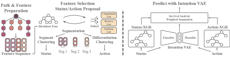
Figure 1. An overview of our Intention Monitor. After extracting address and path features, the model will select and complement the most significant features. Then, a dynamical segmentation module splits the observation period into several coherent segments and maps the segments and their differentiation to a set of global statuses and actions through clustering. Finally, the Intention VAE module weights the contribution of status/action and then fine-tunes the weighted summation of two XGB models’ predictions.

• Early detection is all that matters. Unlike all other traditional financial assets, cryptocurrencies are traded at a 24/7, never-sleeping pace. Most malicious behaviors last for a short duration, measured only by hours, and will have already inflicted the damage before the associated malicious addresses are forever abandoned if they are not detected in the early stage. Moreover, due to the decentralized nature of cryptocurrency’s peer-to-peer transactions, retrospective analysis and identification provide little value as financial losses are almost impossible to be held back and recover once the perpetration is complete. This challenges most existing graph-based methods as transaction graphs (Chen et al., 2020a; Lin et al., 2020a; Francesco Maesa et al., 2016) needed by these methods must be sufficiently large to provide useful structural information (Abay et al., 2019). In most cases, the time it takes to form such a transaction graph is much too long to respond effectively to malicious behaviors in action. Besides, these methods are usually computationally expensive and time-consuming for early-stage detection.

• Type-specific features are not versatile enough for malicious behavior detection. The types of malicious behaviors in cryptocurrencies are increasingly diverse, complex, and constantly evolving, ranging from bitcoin-based scams to darknet markets and modus operandi hacking attacks (Connolly and Wall, 2019). The characteristics of malicious behaviors also vary a lot across different types. Manually-engineered features from specific malicious behaviors cannot be generalized to other types and unknown ones, let alone apply to other cryptocurrencies with a complex heterogeneous relationship in general (Klusman and Dijkhuizen, 2018; Sun et al., 2012). Although some studies (Nerurkar et al., 2020) can detect categories of malicious activities, they are still only available for post-hoc analysis and invariably require a full-history feature observation, which is consequentially scarce at the early stage of these fraud activities. Thus, they cannot be directly deployed to detect illicit activities at the early stage. A more general class of features that capture more fundamental characteristics of malicious behaviors across different types is required to achieve the desired versatility.

• Interpretability is essential. Many malicious behaviors among the cryptocurrency platforms are packaged as commercial projects to lure victims into investing. Investors must be able to investigate and tell real creditable projects from fraudulent ones. However, most detection methods nowadays hardly offer insights into the model’s predictions (Li et al., 2019). In particular, most models tend to improve recall for better safety and work appropriately for the surveillance department. However, it may increase the risk of missing investment opportunities for common investors. From the perspectives of regulators and investors, model interpretability that offers a deeper understanding of the underlying intention behind malicious behaviors is crucial for correctly assessing and identifying malicious behaviors.

Moreover, among all cryptocurrency platforms, Bitcoin (BTC) has the largest volume, while the on-chain record data for a certain address are much scarcer than other popular platforms (e.g., ETH, EOS with smart contracts). Thus, methods proposed on BTC are compatible with those on other cryptocurrency platforms. To address the above-mentioned challenges in cryptocurrency platforms, we propose Intention Monitor on BTC, an early malice detection system based on the notion of asset transition paths. The essential idea is based on the fact that, no matter which malicious behavior, the ultimate motivation and damage are reflected in the significant asset transition between innocent addresses and malicious ones. Patterns extracted from significant asset transition would therefore reveal the intention of malicious behavior across different types. Due to the generality of our asset transition paths, our Intention Monitor is potentially applicable and compatible with domain-specific techniques in other cryptocurrencies. On a high level, our solution progresses in the following four stages:

(I) Feature formation. As shown in Fig.1, firstly, long-term (LT) and short-term (ST) transition paths, the features of the greatest descriptive power and versatility for early-stage malice, would be generated to capture the transaction patterns for both LT and ST transition structures.

(II) Feature selection and complement. Secondly, a Decision-Tree based Feature Selection and Complement (DT-SC) module would identify features of the best discriminative power for different malicious behavior types.

(III) Temporal assembly and semantic mapping. Status/Action Proposal Module (S/A-PM) dynamically assembles the observation period into several temporally coherent segments. It then maps all temporally coherent feature segments to a global status set through clustering. Also, the differentiations between consecutive segments are mapped to global action clusters. These statuses and actions constitute the semantic units, and a status-action tuple (status, action) is used to denote the corresponding intent-snippet at the same time step.

(IV) Model training with intention motif as prediction witness. Status-based and action-based XGB models are trained to give backbone predictions. The hidden intent-snippet embedding will be proposed by the Intention-VAE module to weight the contribution of the two backbone predictions. Furthermore, these hidden snippet embeddings are used to fine-tune the predictions with a survival module and sequence into intention motifs which serve as a witness to the prediction result.

To summarize, the key contributions of this paper are as follows:

• We propose a novel definition of asset transfer path, which is effective in capturing BTC transaction patterns for early malice detection and applicable to other cryptocurrencies potentially, making the versatility of the model across different malicious behavior types possible.

• We provide good interpretability for our malice detection result with intention motif as prediction witness, which is unachievable by those entire deep-learning models. This is achieved by a combination of (I) our DT-SC module to select features and S/A-PM to assemble the observation period and propose statuses, actions, and intent-snippets. (II) an Intention-VAE module which encodes intent-snippet into hidden embeddings to weight the contribution of different information dynamically, and (III) the survival module of Intention-VAE to fine-tune the backbone predictions and group intent-snippets into the sequence of intention motif.

• We conduct extensive evaluation and perform substantially better on three malicious data sets than the state-of-the-art. Furthermore, we present a deep-dive case study on the 2017 Binance hack incident to illustrate the corroborating transaction patterns and unexpected hidden insights for early-sate malice detection that are otherwise unattainable.

2. Related Work

There are many crimes involving many addresses on cryptocurrency trading platforms. Therefore, detecting the identity information of the address is of great significance to the event’s post-analysis and early prediction. Based on the types of features, we divide the existing malicious address detection methods into three categories: (1) case-related features; (2) general address features; (3) network-based features.

2.1. Case-Related features

Case-related features model the addresses and activities in a specific event. These detailed analyses are based on the IP addresses of object nodes, public data from exchanges, and labels from related forums. Concretely, some victims provided the criminals’ addresses and the detail of the criminal cases they experienced. Except for those detailed data, the time difference between illegal transactions and the sub-structure in criminal cases is also helpful in malice-case analysis. Reid and Harrigan (Reid and Harrigan, 2013) combined these topological structures with external IP address information to investigate an alleged theft of BTC. To extract information from social media, a transaction-graph-annotation system (Fleder et al., 2015) is presented. It matched users with transactions in darknet organizations’ activities. Similarly, by exploiting public social media profile information, in (Al Jawaheri et al., 2020), they linked 125 unique users to 20 hidden services, including Pirate Bay and Silk Road. Marie and Tyler (Vasek and Moore, 2015) presented an empirical analysis of BTC-based scams. By amalgamating reports in online forums, they identified 192 scams and categorized them. Instead of direct numerical analysis, other prior studies (McGinn et al., 2018, 2016) detected three anomalous “worm” structures associated with spam transactions by visualizing the transaction data. The case-related features are often helpful in specific case studies. However, most insights are only available in particular cases and can not be generalized to other issues. Thus, we put forward the asset transition paths, which are general in all event analyses.

2.2. General address features

The case-dependent criminal knowledge should be generalized to criminal patterns for a more general detection system. Many works resort to machine learning for malicious activities and illegal address detection. The first step for a machine learning model is a feature proposal module (Monaco, 2015). Since the transaction is the only possible action for a BTC address, commonly used address features majorly describe related transactions, revealing behavior preferences for the given address. Elli et al. (Androulaki et al., 2013) proved transaction patterns such as transaction time, the index of senders and receivers, and the amount value of transactions can help reveal addresses’ identity. Francesco et al. (Zola et al., 2019) proposed a method for entity classification in BTC. By performing a temporal dissection on BTC, they investigated whether some patterns are repeating in different batches of BTC transaction data. On ETH, Chen et al. (Chen et al., 2018, 2019) extracted features from user accounts and operation codes of the smart contracts to detect latent Ponzi schemes implemented as smart contracts. Considering the intrinsic characteristics of a Ponzi scheme, the extracted features mainly describe the transaction amount, time, and count in a specific period. Yin et al. (Yin and Vatrapu, 2017) applied supervised learning to classify entities that might be involved in cybercriminal activities. Akcora et al. (Akcora et al., 2019) applied the topological data analysis (TDA) approach to generate the BTC address graph for ransomware payment address detection. Shao et al. (Shao et al., 2018) embedded the transaction history into a lower-dimensional feature for entity recognition. Nerurkar et al. (Nerurkar et al., 2020) used $9$ features to train the model for segregating $28$ different licit-illicit categories of users.

The proposal of the address feature has significantly improved the model’s generality. However, address features are challenging to characterize the behavioral characteristics of addresses immediately. Some particular patterns of capital inflow and outflow are difficult to be reflected in these characteristics (e.g., the pyramid structure in the Ponzi scheme and the peeling chain in money laundering). Moreover, the discriminative features are various from type to type. The redundant features are essential noise for detection. Therefore, based on the asset transition path, we propose forward and backward concepts to describe the inflow and outflow of the asset. Furthermore, our DT-SC can propose the best feature sets for different types of activities.

2.3. Network-based features

Cryptocurrency inherently provides a transaction network between addresses. Besides focusing on address-level information, network-based features aim to characterize abnormal addresses from network interaction behaviors. By building an address or transaction network, graph metrics are proven powerful in detecting malicious activities. By taking advantage of the power degree laws and local outlier factor methods on two BTC transaction graphs, Pham and Lee (Pham and Lee, 2016) detected the most suspicious 30 users, including a justified theft. Ranshous et al. (Ranshous et al., 2017) analyzed the transaction patterns centered around exchanges. Their study introduces various motifs in directed hypergraphs, especially a 2-motif as a potential laundering pattern. Wu et al. (Wu et al., 2021) proposed two kinds of heterogeneous temporal motifs in the BTC transaction network and applied them to detect mixing service addresses. EdgeProp (Tam et al., 2019), a GCN-based model, was proposed to learn the representations of nodes and edges in large-scale transaction networks. Lin et al. (Lin et al., 2020b) analyzed two kinds of random walk-based embedding methods that can encode some specific network features. Weber et al. (Weber et al., 2019) encodes address transaction graph with GCN, Skip-GCN, and Evolve-GCN. Chen et al. (Chen et al., 2020c) proposed E-GCN for phishing node detection on the ETH platform. By changing the sampling strategy in Node2Vec, Wu et al. (Wu et al., 2020) proposed the Trans2Vec model, which can consider the temporal information. Li et al. (Li et al., 2022) used TTAGN to model the temporal information of historical transactions for phishing detection.

Network-based methods perform well for retrospect analysis, as they encode the structural information of transaction graphs. However, in the early stages, to hide their identities, malicious addresses often transfer their asset with a chain-like structure. Moreover, the trading network is often too small to form a discriminative topological structure. Also, these methods may lead to over-smoothing issues and the dilution of the minority class (Liu et al., 2021a) under the data-unbalanced setting.

3. Problem Formulation

3.1. Problem Definition

In examining each BTC transaction, denoted as $tx$, we break down its input transaction set $I$= $\{i_{1},i_{2},\dots,i_{|I|}\}$ and output transaction set $J$= $\{j_{1},j_{2},\dots,j_{|J|}\}$. The transaction $tx$ accounts for the redistribution of tokens between sets $I$ and $J$. To visualize it, think of incoming tokens pouring into a reservoir before being allocated to the outgoing transactions based on predetermined ratios. As shown in Fig. 2, there are five input transactions and two output transactions in this example.

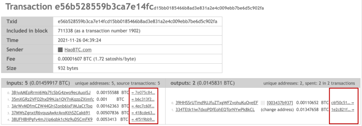
Figure 2. A BTC transaction example. The strings on the red boxes stand for $5$ input transactions and $2$ output transactions.

However, there is no explicit record of the number of tokens moving from an input $i$ to an output $j$. This necessitates the creation of a complete transaction bipartite graph for this $tx$, ultimately leading to the generation of $|I|\times|J|$ transaction pairs. Put simply, a single transaction houses $|I|\times|J|$ transaction pairs within it.

By the $t_{m}$-th time step, let $D_{t_{m}}$=$\{d^{i}_{t_{m}}\}_{i=1}^{N}$=$\{(l^{i},T_{in,t_{m}}^{i},T_{out,t_{m}}^{i})\}_{i=1}^{N}$, where $l^{i}\in\{0,1\}$ is the label of address $i$, $0$ and $1$ stand for regular and malicious addresses respectively. $T_{in,t_{m}}^{i}$=$[tx_{in,1}^{i},tx_{in,2}^{i},\dots tx_{N_{in,t_{m}}}^{i}]$ are transactions where address $i$ acts as the input address, and $T_{out,t_{m}}^{i}$ is the transaction set where address $i$ acts as the output address by the $t_{m}$-th time step. For ease of understanding, we denote these two transaction sets as the $receive$ set and $spend$ set, respectively.

Early Malicious Address Detection (EMAD). Given a set of addresses $A$, and $D_{t_{m}}$ at $t_{m}$-th time-step, the problem is to find a binary classifier $F$ such that

(1) $$F(d^{i}_{t_{m}})=\begin{cases}1&\text{if address $i$ is illicit}\\ 0&\text{Otherwise}\end{cases}.$$

In the early detection task, we require the prediction to be consistent and predict the correct label as early as possible. We denote the confident time as $t_{c}$, where all classifier’s predictions $F$ after $t_{c}$ are consistent. The smallest $t_{c}$ is denoted as $t_{f.c}$. We aim to train a classifier to predict the correct address’s label with the smallest $t_{f.c}$.

3.2. Solution Overview

Inspired by prior research on illegal activity intention encoding (Liu et al., 2021b, 2020), we develop a novel solution, Intention Monitor, for the early detection of malicious addresses.

In particular, as shown in Fig. 3, we propose asset transfer paths to describe the transition patterns. These asset transfer paths can essentially capture the transaction characteristics and address intentions by tracing the source and destination of every related transaction.

Next, we put forward a Decision-Tree based Feature Selection and Complement model (DT-SC) where a decision tree model is deployed to filter and complement the most significant features for different types of malicious behaviors. Based on the features selected by DT-SC, the Status/Action Proposal Module (S/A-PM) divides the observation period into several segments dynamically. Then, S/A-PM clusters all the addresses’ segment representations and presents a set of global status representations. The global action representations are proposed similarly based on the differentiation between two consecutive segment representations. Each segment now has global status, action, and the corresponding intent-snippet, which can explain the behavioral intention of a given address. Based on the status and action vectors, the status and action XGB models are trained to predict status-based and action-based predictions.

Finally, we build Intention-VAE, an efficient early malicious address detection framework. The framework can (1) comprehensively encodes the relationship between status and action to generate the hidden intent-snippet embedding, (2) dynamically weights the contribution between the status and action XGB models, (3) fine-tune the weighted backbone predictions and group intent-snippets into the sequence of intention motifs. In the subsequent sections, we introduce asset transfer path, DT-SC with S/A-PM, and Intention-VAE in Sections 4, 5, and 6, respectively.

4. Asset Transfer Path

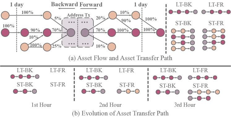
Figure 3. (a) Address transaction flow and asset transfer paths. Numbers are the amount proportions to the destination/source node. $LT$, $ST$, $FR$, and $BK$ are long-term, short-term forward, and backward, respectively. (b) Evolution of asset transfer path. New asset transfer paths are generated if the address participates in new transactions. Forward paths can be extended if the asset continues to flow in the next period.

At the early stage of malicious behaviors, the address-based network has not grown to the size for a credible prediction. Instead, the transaction flow can provide critical information during this period. We design asset transfer paths that consist of significant transactions for the EMAD task.

As mentioned in Sec. 3, there are $|I|\times|J|$ transaction pairs in one BTC transaction. However, not all transaction pairs are helpful for malicious address detection. Those important transactions typically constitute a significant portion of the entire transaction amount. We call such transactions significant transactions. As illustrated in Fig. 3, each node represents a transaction. The nodes inside the dashed gray box stand for transactions that the given address participates in. The left node is the address’s receive transaction, where the address receives tokens from other transactions. In this single transaction example, there are three inputs, contributing $5\%$, $70\%$, and $25\%$ to the total transaction amount. Similarly, the right node is the address’s spend transaction, where the address transfers its tokens to the outputs. This transaction involves multiple outputs (with a distribution of $20\%$, $70\%$, and $10\%$ as in this example). We then propose influence and trust transaction pairs.

4.1. Influence transaction pair

Given an input set $I$= $\{i_{1},i_{2},\dots i_{|I|}\}$ to an output $j$ and the transaction pair set is $\{{I\rightarrow j}\}$, i.e., $\{{I\rightarrow j}\}$=$\{(i_{1},j),(i_{2},j),\ldots,(i_{|I|},j)\}$, we define influence transaction pair as follows: Given an influence activation threshold $\theta$, $(i_{k},j)$ is called an influence transaction pair for transaction $j$, if there exists a $k$ ($1\leq k\leq|I|$) such that the amount of transaction pair $(i_{k},j)$ contributes to at least a certain proportion of the input amount of transaction $j$, i.e, $\hat{A}(i_{k},j)\geq\theta\times\hat{A}(\{{I\rightarrow j}\})$, where $\hat{A}(\cdot)$ denotes the amount of a transaction pair or the sum of all transaction pairs.

Given an influence transaction pair $(i_{k},j)$, we can conclude that output $j$ obtains at least a significant amount (based on the threshold) of the asset in this transaction from input $i_{k}$. Accordingly, given an receive transaction $j$ for the given address, to trace back to the source of the asset, we proposed backward path based on influence transaction pair. Algo. 1 gives the detail to prepare backward paths that reveal where $j$ obtains the asset.

4.2. Trust Transaction Pair

In addition to tracing back to the asset source, we also need to investigate where the asset flows to, i.e., the destination of the asset transfer. To that end, we define trust transaction pair as follows: Given a set of outputs $J$= $\{j_{1},j_{2},\dots j_{|J|}\}$, an Input $i$, and the set of all transaction pairs $\{{i\rightarrow J}\}$, for an output $j_{k}$ ($1\leq k\leq|J|$), if the input $i$ transfers at least a certain proportion of its output amount to it, this transaction pair is called a trust transaction pair for Input $i$. It indicates a specific form of trust from $i$ to $j_{k}$ in an asset transfer.

Given a trust transaction pair $(i,j_{k})$, we can conclude that input $i$ sends a certain degree of the asset to output $j_{k}$. To trace the destinations of Input $i$, we also define forward paths based on trust transaction pair. The pipeline to construct forward path is similar to backward path. The only difference is the tracing direction.

input : Initial Output Tx $j^{o}$, Threshold $\theta$, Time Span $T_{Span}$.

output : Backward Path Set $P$.

1Initialize Backward Path Set: $P\leftarrow\{[-,1,j^{o}]\}$;

2 Initialize Previous hop recorder: $P_{pre}\leftarrow\{[-,1,j^{o}]\}$;

3 Initialize Ending Flag: $F_{end}\leftarrow False$;

4 $j^{o}$’s Time: $T_{j^{o}}\leftarrow$ Time of $j^{o}$;

5while $F_{end}\neq True$ do

      6 Current hop recorder $P_{now}\leftarrow\{\}$;

      7 $F_{end}\leftarrow True$;

      8 for $p$ in $P_{pre}$ do

            9 $j\leftarrow$ Output Tx $p[2]$;

            10 $I\leftarrow$ Input Tx Set of $j$;

            11 for $i$ in $I$ do

                  12 $Prop_{i}\leftarrow Amt_{i}/Amt_{I}$;

                  13 $Score_{i}\leftarrow Prop_{i}*p[1]$;

                  14 $T_{i}\leftarrow$ time of $i$;

                  15 if ($Score_{i}\geq\theta$ and $T_{j^{o}}-T_{i}\leq T_{Span}$) then

                        16 Append $[j,Score_{i},i]$ to $P_{now}$;

                        17 $F_{end}\leftarrow F_{end}$ $\&\&$ $False$;

                  

            

      18$P_{pre}\leftarrow P_{now}$;

      19 $P\leftarrow P\cup P_{pre}$;

      

20return $P$

Algorithm 1 Backward path preparation

4.3. Long-term and Short-term Path

For brevity, we would refer to both the backward path (BK) and forward path (FR) as asset transfer paths and the activation threshold in both directions as activation threshold. To delineate the transaction patterns of an address at both macro and micro levels for both backward path and forward path, we define two kinds of time spans, i.e., long-term and short-term.

Long-term (LT) asset transfer paths have a larger maximum observation period and higher activation threshold, as they are designed to find the transaction’s major asset source. Short-term (ST) asset transfer paths have a shorter observation period and lower activation threshold. They describe the transition pattern and structure (e.g., pyramid-shaped, pulse-shaped, and spindle-shaped) within a short period.

5. Feature Selection and Complement & Status Proposal Module

input : Initial feature list $F^{i}$, Threshold $\theta$.

output : Complement, Reserve, and Delete lists $F_{C},F_{R},F_{D}$.

1 Complement and Delete feature list: $F_{C},F_{D}\leftarrow\{\}$;

2 Reserve feature list: $F_{R}\leftarrow F^{i}$;

3 Average performance score: $s_{p}^{A}\leftarrow 0$;

4 Best average performance score: $s_{p}^{B,A}\leftarrow 0$;

5while $s_{p}^{A}\geq s_{p}^{B,A}$ do

      6 $s_{p}^{B,A}\leftarrow s_{p}^{A}$;

      7 $F^{tmp}_{C},F^{tmp}_{R},F^{tmp}_{D}\leftarrow F_{C},F_{R},F_{D}$;

      8 Average performance score $s_{p}^{A}\leftarrow 0$;

      9 Best performance score $s_{p}^{B}\leftarrow 0$;

      10 for $idx\leftarrow 1$ to $10$ do

            11 $DT_{idx},s_{p,idx}\leftarrow$ Train&Test DT($F_{C},F_{R},F_{D}$);

            12 $s_{p}^{A}\mathrel{+}=s_{p,idx}/10$;

            13 if $s_{p,idx}>S^{B}_{p}$ then

                  14 Update($F^{tmp}_{C},F^{tmp}_{R},F^{tmp}_{D}$);

            

      

      15if ($s_{p}^{A}\geq s_{p}^{B,A}$) then

            16 $F_{C},F_{R},F_{D}\leftarrow F^{tmp}_{C},F^{tmp}_{R},F^{tmp}_{D}$;

            

      

17return $F_{C},F_{R},F_{D}$

Algorithm 2 DT-Based Feature Selection and Complement

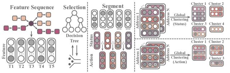
Figure 4. An overview of Decision-Tree based feature Selection and Complement (DT-SC) and Status/Action Proposal Module (S/A-PM). After extracting address and path features, The DT-SC will filter and complement the most significant features. Then, the S/A-PM splits the observation period into several coherent segments and maps the segments and their differentiation to a set of global statuses and actions through clustering.

In this section, we describe the process of Decision-Tree based Feature Selection and Complement (DT-SC) and Status/Action Proposal Module (S/A-PM). We first introduce the address and asset transfer path features. Then, we elaborate on DT-SC that filters, and complements the features for different malicious activities. The status and action sequences are necessary to understand the address’s intention. To fetch these sequences, we deploy S/A-PM to split the observation period into segments and cluster them to generate global status and actions. The overview of DT-SC and S/A-PM is shown in Fig. 4.

5.1. Address & Transaction Features

Table 1. Feature counting and explanation.

Feature Type	Aspect	Feature	Num.	Complement
Address	Balance	Balance	1	None
	Tx Count	Number of spend (receive) tx (by now/recent one hour)	4	None
		Ratio of spend tx to recieve tx (by now/recent one hour)	2	None
	Tx Frequency	Max spend (receive) tx number per hour	2	None
	Abnormal Tx	Number of spend (receive) tx with 0 amount	2	None
	Temporal Info	Time of max hourly spend (receive) tx number	2	None
		Time difference between max hourly spend and receive	1	None
	Activity	Active hour number and active rate	2	None
Path	Path-Count	Path number	1	None
	Path-Length	Hop (height)-length	2	Min,Max,Std
(LT/ST)-(BK/FR)	Tx Amount	Max (min) input (output) amount	4	Min,Max,Std
	Tx Structure	Max (min) input (output) tx number	4	Min,Max,Std
	Connectivity	Path’s max (min) activation score	2	Min,Max,Std

Following (Bartoletti et al., 2018; Nerurkar et al., 2020; Aziz et al., 2022), we also use the address features to characterize the address’s behaviors. As shown in Table LABEL:tab:feat_explain, we extracted 16 address features that characterize an address from six perspectives. Moreover, the asset path can provide critical information. For a specific path set, we selected 13 path features from five perspectives. Also, an address has four path sets (LT-BK, ST-BK, LT-FR, ST-FR), a path set has multiple paths, and every path has these 13 path features. To characterize the overall properties of each path set, we calculated the maximum (max), minimum (min), average (avg), and standard deviation (std) values of every feature except the path number. Thus, there are 12*4+1=49 path features for a single path set. Since we have four path sets (LT-F, LT-B, ST-F, ST-B) (Fig. 3), there are 49*4=196 path features in total. We can characterize the early behavior of different types of addresses through these address and path features.

We believe that hundreds of extracted address and path features can summarize addresses’ early behaviors from several perspectives. But for a specific type of activity, not all features are equally helpful, and the introduction of irrelevant features can affect the model’s performance (will be justified in Section 7.3). Therefore, we need to select the most discriminative features from all these features.

5.2. DT-based feature Selection and Complement

Decision trees can partition the data based on the features that best separate the classes or target variables. During the tree-building process, features that are more informative or discriminatory tend to be selected earlier as splitting criteria. This means that important features are prioritized in the decision tree construction and thus have higher importance scores.

We develop a decision tree-based feature selection and complement module. In this module, we have three sets: complement list, reserve list, and deletion list. This module complements features in the complement list, retains features in the reserve list, and deletes features in the deletion list.

In the initial round, address features and all path features’ mean values are set as seed features. So the seed feature number is 13*4+16=68. We feed these 68 features into the decision tree model and select the best-performing (the performing score will be elaborated in Section 7.2) model from $10$ independent training models. We sort the model’s feature importance scores and denote the maximum importance score as $s_{imp}^{M}$. Given a feature j with an importance score $s_{imp,j}$, if $s_{imp,j}$$\geq$$\theta$*$s_{imp}^{M}$, we append it into the complement list and complement it in the next round of training. $\theta$ is the complement threshold. If $0<s_{imp,j}<\theta$*$s_{imp}^{M}$, we append it into the reserve list, and we will retain it without complement in the following round. If $s_{imp,j}$=$0$, we append it into the deletion list, and we will delete this feature in the subsequent training process.

In the second round of training, we first complement the features in the complement list. Here, by complement, we mean not only using the feature’s mean value but also including its maximum, minimum, and standard deviation (only path features are available for complement). Through complement, we provide the model with more details about the complement feature. Then, we append reserve features to the input feature list without changing them. Finally, we delete features in the delete list. Algo. 2 shows the details of DT-SC.

5.3. Status/Action Proposal Module

The status and action sequences can depict the intention of the given address (Liu et al., 2021b), which is of great importance to the model’s interpretability. However, if we analyze each address independently, it is difficult for the model to obtain a generalizable intention module, the model’s ability and interpretability will be reduced when predicting newly emerging malicious behaviors. To solve these problems, we propose the Status/Action Proposal Module (S/A-PM).

Dynamical segmentation. By definition, status is to describe a certain stable state. To characterize the statuses and their evolution, we need to split the entire observation time window into several “state” segments dynamically. In every segment, we require all addresses’ features to be stable enough. Therefore, at the $J$-th time step, we first normalize all addresses’ feature sequences along the timeline. Take address $i$ as example, the feature list is $[f_{1,i},...,f_{j,i},...f_{J,i}]$ where $f_{j,i}$ is the feature vector at $j$-th time step of address $i$. And for each time step $j$, we then calculate the change ratio $C_{j}$.

(2) $$C_{j}=\frac{\sum_{i=1}^{N}{\sum_{m=1}^{M}({f_{j,i}^{m}-f_{j-1,i}^{m}})/({f_{j-1,i}^{m}+{\delta}})}}{M*N},$$

where $N$ is the data size, $M$ is the feature dimension, $delta$ is a small number in case of the divisor equals $0$. By the $J$-th time step, the highest and current change ratio is denoted as $C_{H}$ and $C_{J}$. If $C_{J}>\theta*C_{H}$, we think the addresses’ statuses change and add $J$ to the segmentation point list. In this manner, we can guarantee the stability of each segment. Notice that, to build a more general segmentation strategy, the segmentation point list is shared by all addresses.

Segment Representation. Then, to build a generalizable intention module, we need to find and represent the common ground of these segments across all addresses. Therefore, for the $j$-th segment of address $i$, we first define its segment representation. The segment’s beginning and end time points are denoted as $b_{j}$ and $e_{j}$ respectively, and the corresponding feature sequence is $[f_{b_{j},i},f_{b_{j}+1,i},...,f_{e_{j}-1,i},f_{e_{j},i}]$. Then the segment vector $g_{j,i}$ is calculated as the average of the feature sequence over the timeline. Naturally, the change between $g_{j-1,i}$ and $g_{j,i}$ is redeemed as segment differentiation $d_{j,i}$. Specially, we define $g_{0,i}$ as a full-zero vector. Thus, for address $i$, we get a sequence of segment representations $[g_{1,i},...,g_{k,i},...,g_{K,i}]$, and a sequence of differentiation representations $[d_{1,i},...,d_{k,i},...,d_{K,i}]$, where $K$ is the segmentation number.

Status and action clustering. Addresses with the same type may have similar purposes. For example, after the Ransomware addresses are activated, most will wait for the victims to pay the ransom in a segment and transfer out quickly in another segment. We can call these two segments the “waiting segment” and “transfer segment” respectively. These semantic meanings are beneficial for understanding and interpreting the address’s intention, and we will justify this in Section 7.6.

To obtain global semantic representations such as “waiting” or “transfer”, we cluster these $N*K$ addresses’ segment representations through the agglomerative clustering algorithm, a hierarchical clustering method. The hierarchical structure provides better interpretability in further analysis. Similarly, we cluster these $N*K$ addresses’ segment differentiations to describe the general actions to obtain action clusters. We denote each status and action cluster’s centers as the status and action vectors. Finally, for each address, we have five sequences: feature, status(vector and cluster index), and action(vector and cluster index). Notice that the action is calculated from the current status and previous status.

6. Intention VAE

As mentioned in Section 2, tree-based machine learning algorithms have been proven powerful in related tasks about malice detection. However, they are difficult to utilize temporal patterns, which is extremely useful for depicting the address’s intention, especially during the early stage with severe data scarcity. Besides, as there is no early stopping mechanism in the decision tree group, subsequent redundant noise will trigger the issue of inconsistent prediction. Thus, on top of tree-based algorithms (XGB as the backbone), we introduce the Intention VAE module, which can encode such temporal patterns and prevent noise with survival analysis.

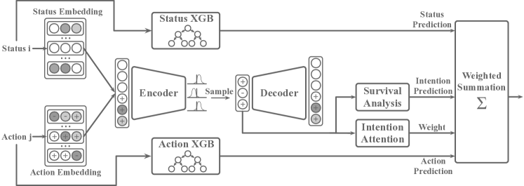
Figure 5. An overview of Intention-Variational-Autoencoder (Intention-VAE). Two XGB models are trained with status and action, respectively. At each time step, the Intention-VAE module generates hidden intent-snippet embeddings to weight the prediction of two XGB models and fine-tunes the weighted prediction.

6.1. Intention Proposal

By understanding an address’s status and action, we can discern its intention. Furthermore, when an address is under a certain status, and its intention is known, we can forecast its subsequent action. Thus, to depict this relationship, we deploy a VAE module to generate the hidden intent-snippets embeddings with the corresponding statuses and actions. As shown in Fig 5, for address $i$ at time step $j$, we have the corresponding status index $S^{idx}_{i,j}$ and action index $A^{idx}_{i,j}$. We transform them into learnable embedding vectors as follows:

(3) $$S^{E}_{i,j} =\mbox{Emb}^{S}(S^{idx}_{i,j}),$$

$$A^{E}_{i,j} =\mbox{Emb}^{A}(A^{idx}_{i,j}).$$

After getting the embedding of status and action, the sampled bottleneck vector of our Intention-VAE module is regarded as the hidden intent-snippet. Through Intention-VAE, we can preserve the most critical information of status and action. Moreover, the non-linear transformation in the module can generate a more expressive representation. Another crucial point is that Intention-VAE can guarantee that the intention space has the properties of continuity and completeness (Kingma and Welling, 2013). Specifically, continuity requires two close intention points in the latent space not to give two completely different contents. As for completeness, it requires an intention point to give meaningful content once decoded. The intention representation is calculated as follows:

(4) $$x_{i,j} =\mbox{VAE-Encoder}([S^{E}_{i,j}||A^{E}_{i,j}]),$$

$$\mu_{i,j} =W_{x{\mu}}x_{i,j}+b_{\mu},$$

$$\sigma_{i,j} =W_{x{\sigma}}x_{i,j}+b_{\sigma},$$

$$z_{i,j} =\mu_{i,j}+\mbox{exp}(\sigma_{i,j})\odot e,\ e\sim\mathcal{N}(0,I),$$

$$\hat{x}_{i,j} =\mbox{VAE-Decoder}(z_{i,j}),$$

where $[.||.]$ stands for concatenation, $\hat{x}_{i,j}\in\mathbb{R}^{d_{z}}$ is the output of the VAE encoder, $d_{z}$ is the dimension of the intent-snippet. $z_{i,j}$ is the bottleneck vector of our Intention-VAE, also denoted as the hidden intent-snippet embedding. Instead of decoding the interval vector directly, VAE encodes inputs as distributions. Thus, the model proposes the mean value $\mu_{i,j}$ and stand deviation $\sigma_{i,j}$. Our hidden intent-snippet embedding is sampled from the distribution of $\mathcal{N}(\mu_{i,j},\sigma_{i,j})$. However, due to the gradient descent issue of the sampling process, the module uses a reparameterization trick to sample $e$ form $\mathcal{N}(0,\mathcal{I})$ instead of sampling $z$ directly. $\hat{x}_{i,j}$ is the reconstruction of input data.

6.2. Intention-Based Survival Analysis

To enable the model to encode temporal patterns, we introduced Intention-Based Survival Analysis to Intention-VAE. This module can accelerate the prediction speed and improve the consistency of the prediction by cutting off continuous noise.

The survival function $S(j)$ represents the probability of an event that has not occurred time step $j$, where an event here represents “the given address labeled as malicious”. Every time step, the model should give lower $S(j)$ to malicious addresses and higher $S(j)$ to legal addresses. The hazard function $\lambda_{j}$ is the instantaneous event occurrence rate at time $j$ given that the event does not occur before time $j$. Note that the observation time is discrete in our case. We denote a discrete timestamp index as $j$, the association between $S(j)$, $\lambda_{j}$ and probability density function $f_{j}$ can be described as:

(5) $$S(j) =P(T\geq{j})=\sum_{k=j}^{\infty}f_{k},$$

$$\lambda_{j} =P(T=j|T\geq{j})={f_{j}}/S(j),$$

$$S(j) =exp({-\sum_{k=1}^{j}\lambda_{k}}).$$

To enable the model to encode temporal patterns, we first update each input with corresponding LSTM modules as follows:

(6) $$h_{i,j}^{F},c_{i,j}^{F} =\mbox{LSTM}^{F}([z_{i,j}||f_{i,j}],h_{i,j-1}^{F},c_{i,j-1}^{F}),$$

$$h_{i,j}^{S},c_{i,j}^{S} =\mbox{LSTM}^{S}([z_{i,j}||S^{vec}_{i,j}],h_{i,j-1}^{S},c_{i,j-1}^{S}),$$

$$h_{i,j}^{A},c_{i,j}^{S} =\mbox{LSTM}^{A}([z_{i,j}||A^{vec}_{i,j}],h_{i,j-1}^{A},c_{i,j-1}^{A}).$$

Then, the hazard rate ${\lambda}_{j}$ and intention-based prediction in our Intention-AVE are given as follows:

(7) $$\lambda_{j} =\sum_{{t}\in\{F,S,A\}}ln(1+exp({W_{i}h_{i,j}^{t}}))),$$

$$P_{i,j}^{I} =[exp({-\sum_{k=1}^{j}\lambda_{k}}),\ 1-exp({-\sum_{k=1}^{j}\lambda_{k}})].$$

6.3. Intention Augmented Prediction Fusion

Despite the difficulty in utilizing temporal patterns, tree-based models can provide better stability under label unbalance settings. To incorporate these benefits, we build an Intention Augmented module upon the tree-based models.

First, we train two XGB models with status and action representations, namely Status-XGB and Action-XGB. For address $i$ at time step $j$, based on the status vector $S^{vec}_{i,j}$ and action vector $A^{vec}_{i,j}$, we first get predictions $P_{i,j}^{S},P_{i,j}^{A}\in\mathbb{R}^{2}$ from these two models as the backbone predictions. Each dimension represents the probability of the corresponding class (0-normal, 1-malicious).

Both status and action can provide critical information for prediction, but their contributions may change dynamically. Therefore, the weights assigned in the two decision trees should also change dynamically. To this end, we use the Intention-Attention module to assign the prediction weights of the two decision trees.

(8) $$a_{i,j}^{S} =W^{a}\mbox{tanh}(W^{f,S}[f_{i,j}||S^{vec}_{i,j}]),$$

$$a_{i,j}^{A} =W^{a}\mbox{tanh}(W^{f,A}[f_{i,j}||A^{vec}_{i,j}]),$$

$$a_{i,j}^{I} =W^{a}\mbox{tanh}(W^{f,I}[f_{i,j}||z_{i,j}]),$$

$${\alpha}_{i,j}^{(S,A,I)} =\mbox{exp}(a_{i,j}^{t})/{\sum_{t}^{{\{S,A,I\}}}\mbox{exp}(a_{i,j}^{t})}.$$

With the acceleration of the Intention-Based Survival Analysis, the final prediction $\hat{P}_{i,j}$ for address $i$ at time step $j$ is given by:

(9) $$P_{i,j} ={\sum_{t}^{\{S,A,I\}}P_{i,j}^{t}*a_{i,j}^{t}},$$

$$\hat{P}_{i,j} =S(j)*P_{i,j}+(1-S(j))*\hat{P}_{i,j-1}.$$

The introduction of survival prediction analysis can correct the prediction errors caused by the lack of temporal information and group statuses into an intention sequence. We denote the time step when the survival probability equals $0$ as $t_{die}$, where the model has collected enough information to predict the malicious address’s label. In other words, the model has figured out the address is malicious. Since VAE makes the distribution of each $z$’s dimension close to $\mathcal{N}(0,I)$, and the intention latent space is continuous and complete, we can binarize each dimension to index each address’s intent-snippet as $I^{idx}_{i,j}$ (e.g., As shown in Fig 5, $z$’s dimension $d_{z}$ is $3$ , we can get $8$ intention indices, i.e., $1$(+,+,+), $2$(-,+,+), …, $7$(+,-,-), $8$(-,-,-)). Thus, we call the intent-snippet index sequence $\{I^{idx}_{i,j}\}^{t_{die}}_{j=1}$ as the intention motif of address $i$. And this intent-snippet motif can be interpreted by the corresponding status and action sequences.

6.4. Loss Function

Classification Loss. For address $i$ at $j$-th time step, the early detection likelihood that this address is malicious and the negative logarithm prediction $loss^{P}$ are defined below:

(10) $$\hat{y}_{i,j} =P_{i,j}[1],$$

$$likelihood =(1-\hat{y}_{i,j})^{l_{i}}({\hat{y}_{i,j}})^{1-l_{i}},$$

$$loss^{P}_{i,j} =({l_{i}}-1)*\mbox{log}({\hat{y}_{i,j}})-{l_{i}}*\mbox{log}(1-{\hat{y}_{i,j}}).$$

Intention-VAE Loss. VAE is trained by maximizing the log-likelihood as follows:

(11) $$\mbox{log}P([S^{E}_{i,j}||A^{E}_{i,j}]) =\int_{z}(q(z|[S^{E}_{i,j}||A^{E}_{i,j}])\mbox{log}P([S^{E}_{i,j}||A^{E}_{i,j}]))dz,$$

$$=\int_{z}q(z|[S^{E}_{i,j}||A^{E}_{i,j}])\mbox{log}(\frac{P(z,[S^{E}_{i,j}||A^{E}_{i,j}])}{q(z|[S^{E}_{i,j}||A^{E}_{i,j}])})dz$$

$$+\int_{z}q(z|[S^{E}_{i,j}||A^{E}_{i,j}])\mbox{log}(\frac{q(z|[S^{E}_{i,j}||A^{E}_{i,j}])}{P(z|[S^{E}_{i,j}||A^{E}_{i,j}])})dz,$$

$$\geq\int_{z}q(z|[S^{E}_{i,j}||A^{E}_{i,j}])\mbox{log}(\frac{P([S^{E}_{i,j}||A^{E}_{i,j}]|z)P(z)}{q(z|[S^{E}_{i,j}||A^{E}_{i,j}])})dz,$$

where $z\sim\mathcal{N}(0,I)$ is an intermediate random variable, $\int_{z}q(z|[S^{E}_{i,j}||A^{E}_{i,j}])\mbox{log}(\frac{q(z|[S^{E}_{i,j}||A^{E}_{i,j}])}{P(z|[S^{E}_{i,j}||A^{E}_{i,j}])})dz$ equals $KL(q(z|[S^{E}_{i,j}||A^{E}_{i,j}])||P(z|[S^{E}_{i,j}||A^{E}_{i,j}]))$ which is guarantee to be positive. Thus we only need to maximize the lower bound $lb_{i,j}$ i.e., the last term in the above equation. $lb_{i,j}$ can be reformalized as follows:

(12) $$lb_{i,j}=\int_{z}(q(z|[S^{E}_{i,j}||A^{E}_{i,j}])\mbox{log}(\frac{P(z)}{{q(z|[S^{E}_{i,j}||A^{E}_{i,j}])}})dz+\int_{z}(q(z|[S^{E}_{i,j}||A^{E}_{i,j}])\mbox{log}(P([S^{E}_{i,j}||A^{E}_{i,j}]|z))dz,$$

where the first term equals to $-KL(q(z|[S^{E}_{i,j}||A^{E}_{i,j}])||P(z))$. To minimize this KL divergence, we need $q(z|[S^{E}_{i,j}||A^{E}_{i,j}]))$ close to $\mathcal{N}(0,I)$. The second term equals the negative reconstruction error in Auto Encoder. Finally, the VAE loss $loss^{V}_{i,j}$ can be represented as $\sum_{d=1}^{d_{z}}(exp(\sigma_{i,j}^{d})-(1+\sigma_{i,j}^{d})+(\mu_{i,j}^{d})^{2})$ as indicated by (Kingma and Welling, 2013).

Consistent and Early Boost Loss. An accurate and reliable model should provide a consistent prediction. For an ideal model, the current prediction should be consistent with the previous prediction every time step. Thus, we introduce the consistency loss $loss^{C}$ to improve the predictions’ conformity:

(13) $$loss^{C}_{i,j}=\begin{cases}0&sign((\hat{y}^{j}_{i}-0.5)*(\hat{y}^{j-1}_{i}-0.5))>=0,\\ 1&else,\end{cases}$$

where $0.5$ is the decision boundary of positive (malicious) and negative (regular).

To accelerate the prediction speed, we need to decrease the survival probability as soon as possible. Thus, we introduced an earliness loss $loss^{E}$. Every time step, the survival probability for positive samples should be as small as possible. The negative samples’ survival probabilities should be as large as possible. For address $i$ at time split $t$, $loss^{E}$ is defined as:

(14) $$loss^{E}_{i,t}=\begin{cases}S_{i}(t)&l^{i}=1,\\ -S_{i}(t)&l^{i}=0,\end{cases}$$

where $l^{i}$ is the label of address $i$.

However, the model is hard to predict the correct labels at the early stage due to data insufficiency. The model can be perturbed by the wrong predictions in the early period. Thus, all the loss items are weighted by $\sqrt{t}$. the overall loss function is defined as:

(15) $$\mathscr{L}=\sum_{t=1}^{t_{M}}\sum_{i=1}^{N}\sqrt{t}(loss^{P}_{i,t}+\gamma_{1}loss^{V}_{i,t}+\gamma_{2}{loss^{C}_{i,t}}+\gamma_{3}{loss^{E}_{i,t}}),$$

where $\gamma_{1}$ to $\gamma_{3}$ are coefficients to control the contribution between $loss^{P}$, $l_{b}$, $loss^{C}$ and $loss^{E}$. $t_{M}$ is the time span of training data, $N$ is the training address number.

7. Experiment and Analysis

7.1. Data Preparation

Raw Data and Label Collection For higher high credibility, we only select data verified by many participants. Thus, we obtained all the data from the $1$-st block to the $610637$-th block (the first block of 2020). To get the labels for three different types of malicious addresses, namely, hack (hack exchanges and steal tokens), ransomware (encrypt victims’ data and demand ransoms in BTC), and darknet (commercial website’s address operates via darknets such as I2P). We performed a manual search on public forums, datasets, and prior studies (Paquet-Clouston et al., 2019), (Li et al., 2020), and (Wu et al., 2021). For regular addresses, we collected four types of addresses as “negative samples”, namely exchange, mining, merchant, and gambling. The negative dataset is also augmented as prior studies (Wu et al., 2021; Liu et al., 2003; Wu et al., 2018; Jaskie and Spanias, 2019). The numbers of positive, negative, positive/negative ratios, and dynamic segmentation numbers (within one day) for each malicious type are shown in Table. 2.

Table 2. Dataset Statistics.

Type	Positive	Negative	Posi./Nega. Ratio	Segment
Hack	341	79,765	0.46%	10
Ransomware	1,903	50,617	3.76%	17
Darknet	7,696	89318	8.62%	18

7.2. Settings and Metrics

Generally, according to public reports, relevant agencies can detect most malicious behaviors within a day, such as hacking or malicious attacks. Therefore, in our experiment, to train a model that gives an early warning, we use address first $24$ hours with a $1$ hour interval as training data. The max time spans for the long-term (LT) and short-term (ST) paths are one week and one day, respectively. Notice that the real timespan for a forward path is the smaller one between observing timestep and the pre-defined max timespan, as we can not foresee future data. We set $0.5$ and $0.01$ as the thresholds for LT and ST paths, respectively, as LT paths aim to find the most critical transaction pairs, and ST paths aim to encode more transaction structure information.

We average the metrics along the timeline to evaluate the performance. The selected metrics are accuracy (Acc.), precision (Prec.), and recall (Rec.). Besides, the model should predict correct labels fast to prevent economic loss earlier. Also, due to data insufficiency, the model may predict conflict labels at different timesteps, thus confusing users. Thus we require the predictions to be consistent. To evaluate the earliness and the consistency of the prediction, we introduce the early-weighted F1 score $F1^{E}$ and consistency-weighted score $F1^{C}$ as follows:

(16) $$\mathit{F1^{E}} =\frac{\sum_{i=1}^{N}{F1_{i}/\sqrt{i}}}{\sum_{i=1}^{N}{1/\sqrt{i}}},$$

$$\mathit{F1^{C}} =\frac{\sum_{i=1}^{N-1}{{\sqrt{i}}\times{F1_{i}}\times{\mathds{1}_{y_{c}}(y_{i})}}}{\sum_{i=1}^{N-1}{{\sqrt{i}}}},$$

where $i$ is the time split index, $y_{c}$ is the prediction set where current prediction $y_{i}$ is consistent with the next prediction $y_{i+1}$. The indicator function $\mathds{1}_{y_{c}}(y_{i})=1$ when $y_{i}\in y_{c}$. $F1_{i}$ is the $F1$ score of the prediction at the $i$-th time split.

7.3. Comparison with State-of-the-art Models

Table 3. Scores of the different prediction models. Inten-M(+Idx) are our Intention Monitor with the intention index embedding. Underline stands for the best score in the group, bold stands for the best score in this dataset.

Dataset	Group	Model	$Accuracy$	$Precision$	$Recall$	$F1^{E}$	$F1^{C}$
Hack	Decision Tree	DT	0.996	0.247	0.051	0.084	0.084
		RF	0.996	0.718	0.134	0.238	0.205
		XGB	0.992	0.081	0.044	0.049	0.048
	Address Graph	GCN	0.736	0.106	0.282	0.163	0.104
		Skip-GCN	0.651	0.143	0.524	0.226	0.125
		Evo-GCN	0.760	0.145	0.335	0.196	0.146
	Sequential Model	GRU	0.970	0.090	0.499	0.133	0.152
		M-LSTM	0.977	0.113	0.445	0.152	0.183
		CED	0.980	0.115	0.401	0.154	0.181
		SAFE	0.974	0.076	0.394	0.133	0.119
		Transformer	0.971	0.094	0.464	0.132	0.157
	Intention Monitor	Status-XGB	0.996	1.000	0.257	0.372	0.390
		Action-XGB	0.996	1.000	0.233	0.370	0.387
		Inten-M	0.996	1.000	0.274	0.412	0.440
		Inten-M(+Idx)	0.997	1.000	0.298	0.436	0.470
Ransomware	Decision Tree	DT	0.964	0.073	0.014	0.025	0.019
		RF	0.964	0.004	0.000	0.000	0.000
		XGB	0.968	0.455	0.421	0.437	0.415
	Address Graph	GCN	0.878	0.223	0.923	0.360	0.359
		Skip-GCN	0.881	0.226	0.910	0.364	0.361
		Evo-GCN	0.866	0.200	0.871	0.322	0.326
	Sequential Model	GRU	0.901	0.280	0.856	0.389	0.355
		M-LSTM	0.919	0.332	0.870	0.443	0.418
		CED	0.921	0.329	0.846	0.442	0.415
		SAFE	0.885	0.246	0.856	0.382	0.294
		Transformer	0.928	0.358	0.853	0.467	0.446
	Intention Monitor	Status-XGB	0.987	0.906	0.724	0.790	0.790
		Action-XGB	0.987	0.910	0.719	0.791	0.780
		Inten-M	0.986	0.930	0.770	0.797	0.801
		Inten-M(+Idx)	0.988	0.889	0.793	0.820	0.824
Darknet	Decision Tree	DT	0.908	0.183	0.012	0.020	0.018
		RF	0.909	0.468	0.013	0.015	0.016
		XGB	0.913	0.571	0.203	0.291	0.278
	Address Graph	GCN	0.841	0.322	0.813	0.463	0.465
		Skip-GCN	0.780	0.260	0.889	0.400	0.404
		Evo-GCN	0.737	0.216	0.822	0.342	0.343
	Sequential Model	GRU	0.874	0.518	0.819	0.601	0.438
		M-LSTM	0.880	0.528	0.822	0.612	0.449
		CED	0.861	0.490	0.835	0.582	0.414
		SAFE	0.828	0.418	0.865	0.557	0.343
		Transformer	0.876	0.515	0.856	0.615	0.438
	Intention Monitor	Status-XGB	0.940	0.796	0.694	0.720	0.608
		Action-XGB	0.941	0.797	0.710	0.727	0.615
		Inten-M	0.945	0.851	0.689	0.736	0.624
		Inten-M(+Idx)	0.945	0.794	0.766	0.762	0.631

To demonstrate the validity of the temporal information, we compare decision tree models, namely Decision Tree (DT) (Liang et al., 2019), Random Forest (RF) (Nerurkar et al., 2020), and XGB (Harlev et al., 2018). Then we compare the address graph-based models to justify the ineffectiveness of most existing graph-based for early detection. Namely GCN, Skip-GCN, and Evolve-GCN in the reference (Weber et al., 2019). To verify the validity of our prediction model, we compare four sequential-based models applied in the “Early Rumor Detection” task, namely GRU (Cho et al., 2014), M-LSTM (Yuan et al., 2017), SAFE (Zheng et al., 2019), CED (Song et al., 2019), and Transformer (Song et al., 2021). For our Intention Monitor, $+Idx$ means we replace $z_{i,j}$ with $[z_{i,j}||\mbox{Emb}^{I}(I^{idx}_{i,j})]$ in Alg LABEL:algo:lstm and Alg 8. ${Emb}^{I}$ is the learnable embedding layer for intention index $I^{idx}_{i,j}$ as mentioned in Section 6.3.

First, as shown in Table 3, our $Inten-M$ model achieves the best performances across all three datasets. The great improvements come from the effective features and our Intention-VAE module. All these compared models also achieve far better performance with our path features and DT-SC module, which will be discussed later.

For all traditional decision tree algorithms, they do not perform well on the three datasets. Because these algorithms are difficult to encode temporal information, it is difficult for decision-tree-based machine learning algorithms to consider shifts in the feature decision boundary. Also, the address features can not provide efficient information for more accurate prediction, thus, even using decision trees as the backbone, our model still improves $F1^{E}$ and $F1^{C}$ significantly compared to the best decision-tree-based model. For address graph methods, as (Liu et al., 2021a) implies, the Address-GCN may lead to over-smoothing issues and the dilution of the minority class. In our cases, most neighbors of malicious nodes are victims or shadow addresses. In addition, since the transaction network is usually small in the early stage of the address, there are many shadow addresses in this network, which makes the Address-GCN models challenging to obtain valuable transaction pattern information. Thus the models do not perform well.

Rather than focusing on the address transaction graph’s structure, sequential models encode the temporal pattern more directly. As shown in Table. 3, compared to the best Address-GCN model, they have an average improvement of $9.76\%$ and $15.78\%$ in $F1^{E}$ and $F1^{C}$ on the three datasets. This improvement verifies the effectiveness of temporal patterns. However, malicious behavior generally involves many transactions, which are often not directly related to the target address. For example, the malicious address will use many shadow addresses for transit. Therefore, the address feature cannot reflect the actual attributes of the address in time, while our backward path feature can describe how the funds flow into the address. Similarly, the malicious address may also transfer funds in a certain way. The most common method is the peeling chain. Our forward path feature can provide relevant information, which is a challenging task for address features. As shown in Table. 3, with the intention attention module, the model can finetune the predictions of $Status$-$XGB$ and $Action$-$XGB$, thus achieving better performance across all three datasets. Compared to the best sequential model, our $Inten$-$M$ model can achieve an average improvement of $93.68\%$ and $94.04\%$ on $F1^{C}$ and $F1^{E}$, proving the great effectiveness of our path feature and corresponding feature selection. Also, the encoding of the binarized Intention index improves the model’s performance one step further, which justifies the boundary in the Intention-VAE module is useful for prediction.

7.4. Feature Combination and Selection

In this subsection, we evaluate the effectiveness of our path features and feature selection scheme. We also justify the generality with compatible models.

Feature Combination. To verify the effectiveness of path features, we compare three decision tree models, namely the address feature (AF) model, the long-term path features (+LT) model, and the short-term path features (+ST) model. +X means add feature X to previous model. As shown in Table 4, AF performed poorly on the three datasets. Path features significantly improve the performance for all metrics. We speculate that most malicious addresses require victims to transfer money once they are created. It makes them similar to exchange or financial service addresses in the early stage. For example, exchange or merchant services will also create new addresses for security. As a result, AF model can only find those extremely abnormal addresses, which results in poor performance.

Feature Selection. Feature selection is crucial for the model’s generalization ability. To justify the effectiveness of our feature selection scheme, we also compare the T/C model with the one without a selection scheme +ST. Trimming scheme (T) stands for trimming off features in the deletion list, Complement scheme (C) stands for complement features in the complement list. As shown in Table 4, feature selection significantly improves the performances of decision trees across all the datasets. The $F1^{C}$ and $F1^{E}$ are enhanced by an average of $13.88\%$ and $9.33\%$, respectively. The major improvement comes from the recall score. Since malicious activities behave abnormally in various aspects, their most significant features are also different. Through our automatic feature selection method, models can fully use the powerful path features. Also, they can adapt to different malicious activities easily, mitigate input noise, and significantly reduce the workload of manual selection.

Since our feature selection scheme is based on the decision tree model, we implement them on other compatible models to verify the generalization of path features and the feature selection scheme. As shown in Table 4, our path feature and feature selection scheme improve the performance for all models. Especially for the decision tree model, the augmented XGB model even outperforms most sequential models.

Table 4. Scores of different features (address feature (AF), long-term path features (+LT), short-term path features (+ST), and selection schemes(trimming/complement scheme (T/C). $\Delta$ stands for performance differentiation after applying path features and selection schemes.)

Dataset	Model	$Accuracy$	$Precision$	$Recall$	$F1^{E}$	$F1^{C}$
Hack	DT(AF)	0.996	0.247	0.051	0.084	0.084
	DT(+LT)	0.995	0.221	0.053	0.079	0.092
	DT(+ST)	0.996	0.882	0.116	0.249	0.278
	DT(+T/C)	0.996	0.821	0.155	0.259	0.277
	RF($\Delta$)	+0.000	+0.282	+0.053	+0.095	+0.093
	XGB($\Delta$)	+0.004	+0.919	+0.181	+0.291	+0.333
	GRU($\Delta$)	+0.018	+0.103	-0.134	+0.089	+0.105
	M-LSTM($\Delta$)	+0.014	+0.184	-0.116	+0.114	+0.134
	CED($\Delta$)	+0.006	+0.044	-0.050	+0.037	+0.040
	SAFE($\Delta$)	+0.006	+0.025	+0.004	+0.034	+0.034
	Transf.($\Delta$)	+0.018	+0.089	-0.176	+0.067	+0.070
Ransomware	DT(AF)	0.964	0.073	0.014	0.025	0.019
	DT(+LT)	0.965	0.313	0.090	0.125	0.126
	DT(+ST)	0.967	0.592	0.270	0.354	0.330
	DT(+T/C)	0.968	0.616	0.399	0.463	0.417
	RF($\Delta$)	+0.005	+0.926	+0.269	+0.394	+0.425
	XGB($\Delta$)	+0.014	+0.334	+0.283	+0.295	+0.313
	GRU($\Delta$)	+0.047	+0.169	-0.027	+0.146	+0.186
	M-LSTM($\Delta$)	+0.027	+0.109	-0.038	+0.087	+0.113
	CED($\Delta$)	+0.022	+0.092	-0.026	+0.070	+0.095
	SAFE($\Delta$)	+0.030	+0.065	-0.020	+0.076	+0.073
	Transf.($\Delta$)	+0.023	+0.102	-0.091	+0.067	+0.089
Darknet	DT(AF)	0.908	0.183	0.012	0.020	0.018
	DT(+LT)	0.911	0.593	0.099	0.143	0.140
	DT(+ST)	0.921	0.609	0.404	0.484	0.452
	DT(+T/C)	0.922	0.618	0.446	0.517	0.461
	RF($\Delta$)	+0.006	+0.324	+0.428	+0.503	+0.499
	XGB($\Delta$)	+0.036	+0.206	+0.417	+0.380	+0.349
	GRU($\Delta$)	+0.041	+0.112	+0.032	+0.091	+0.094
	M-LSTM($\Delta$)	+0.036	+0.106	+0.036	+0.084	+0.085
	CED($\Delta$)	+0.053	+0.138	+0.002	+0.104	+0.118
	SAFE($\Delta$)	+0.046	+0.087	-0.030	+0.060	+0.081
	Transf.($\Delta$)	+0.035	+0.101	+0.001	+0.071	+0.084

7.5. Effect of Status&Action Cluster Number

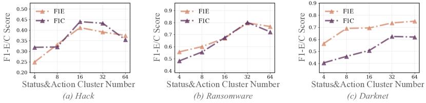
Figure 6. $F1^{E}$ and $F1^{C}$ of different status and action cluster number.

The cluster numbers of status and action represent the granularity of address status and behavior. If the cluster number is too small, it will limit the model’s ability to distinguish and extract adequate information. On the contrary, if the cluster number is too large, it will introduce outliers and deteriorate the model’s interpretability. To this end, we analyze the effect of cluster number on model performance. We test $5$ cluster numbers ($4$,$8$,$16$,$32$,$64$), and the results are shown in Figure  6.

As expected, models with larger cluster numbers can distinguish more states at the beginning and perform better. However, when the cluster number increases, the model may introduce more redundant noise, leading to poor performance. This phenomenon is particularly evident in the hack dataset. This is because compared to other malicious types, hack addresses tend to have fewer actions, so the diversity of their states and actions will be less. Therefore, the best cluster number is $16$, and the performance gradually deteriorates afterward. Moreover, because ransomware and darknet have more operations or requirements for users, the optimal cluster number will be larger. For ransomware, the best cluster number is 32 because it performs best. For darknet, we also choose $32$ as the best cluster number because the performance difference between $32$ and $64$ is marginal. And the model with a smaller cluster number has better interpretability.

7.6. Status Actions and Intention

Differentiation Analysis. We select the top six with the largest differences between malicious and regular addresses. As shown in Fig. 7, the x-axis represents the cluster index of status and action. The y-axis is the discrimination score (the proportion difference between the positive and negative samples divided by the sum of the proportion). A higher score means the cluster appears more in a specific class.

We can see that some status and action clusters can be used as effective discriminant indicators for hack and ransomware addresses. Especially for status 29 in the ransomware dataset, the discrimination score is 1. That is to say, as long as status 29 appears in the address status sequence, the model can confidently determine the address’s label.

As for the darknet address, since its operation method is similar to the typical trading platform, therefore, the cluster discrimination ability is not as strong as the other two data sets. However, when we analyze 2-gram and 3-gram (a contiguous sequence of 2 and 3 cluster indices), we found that the order in which each cluster appears in status and action can give a higher discrimination score for darknet addresses. On the one hand, this justifies the importance of temporal information. On the other hand, it shows that our status and action can be well combined with timing analysis to achieve better results.

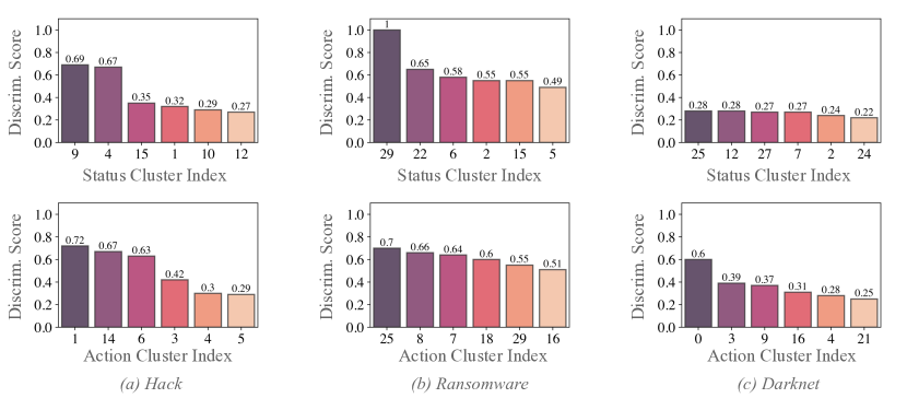
Figure 7. Top-6 differentiated status and action. Labels on the x-axis stand for the index of status and action. The value above each bar is the corresponding discrimination score.

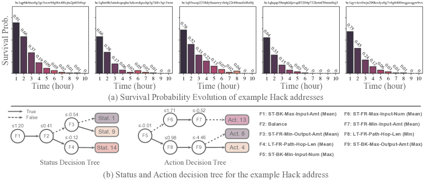
Figure 8. (a) Survival probability evolution of example hack addresses. (b) Status and action decision tree for the example hack address.

Case Study. We use the infamous hack incident of the Binance crypto exchange on May 7, 2019, in which hackers stole over 7000 BTCs worth of 40 million, as a case study to illustrate our model’s capability to interpret prediction result and offer valuable insights into the malicious behavior.

As shown in Fig. 8 (a), our method successfully detects the 5 sample hacker addresses involved by the end of the first $9$ hours since its creation, which is 12 hours before the stolen BTCs were transferred away. We quote from a Binance statement that ”It was unfortunate that we were not able to block this withdrawal before it was executed.”, an inevitable tragedy with only retrospective analysis but totally preventable with our early detection.

To interpret our prediction result, we first zoom into one of the hacker’s addresses bc1***6xp. The prediction result can be easily interpreted by examining the semantics behind the status and action that form the intention motif. By the $16$-th hour, the corresponding status and action sequences are $[1-9-9-9-9-9-9-9-9-9-9-9-9-9-9-14]$ and $[8-8-8-8-8-8-8-8-8-8-8-8-4-8-8-13]$. To interpret the semantic meaning of status and action, we build corresponding status and action decision trees. Take status as an example. After obtaining all the status vectors via clustering, we categorize all the statuses using the decision tree (the number of statuses is equal to the number of categories). Each status can be interpreted by trailing the corresponding decision tree from the root to the leaf, as shown in Fig. 8 (b).

Regarding feature 2, the status decision tree judges ”when the input volume of each ST-BK path is not very large, whether the balance can reach a certain amount.” That is to say, is it in a state of ”remitting funds through multiple channels and having enough balance”? Status 1 essentially indicates that the initial balance is very high, and the asset comes from lots of ST-BK paths. Status 9 mainly determines whether the address has transferred out the asset. As shown in Figure7, there is already a relatively high discrimination score for statuses 1 and 9. Our model can give the correct prediction before the end of status 9, which justifies the effectiveness of our status proposer. Furthermore, at the $16$-th hour, the address status is 14. Status 14 implies that the funds come through multiple ST-BK paths, but the balance is insufficient. The low balance may be because the volumes of ST-BK paths are insufficient or the address transferred out its tokens with short LT-FR paths.

As for action clusters, Action 8 is a waiting action, which is used to describe that the features of the address are relatively stable without much change. We can also see from the figure that all features on the decision path will not have too large or too small values. Action 4 is similar to action-8. The main difference is that the address introduces a small amount of ST-BK path, which leads to a significant decrease in the overall corresponding feature value. Action 13 mainly describes the property change in the ST-FR path. As shown in Fig. 8 (b), this action describes that the address introduces the ST-FR path, most of which are single chains, and the transfer amount is relatively large.

In reality, this malicious address received a transfer of $555.997$ BTCs at creation through $71$ input transitions, with no output transactions. The status sequence can also be observed in the related transaction, in which the hacker manipulated Binance’s address and divided it into $71$ inputs, each containing $100$ BTCs. This justifies the ”Multi ST-BK Paths” property of Statuses 1 and 9. The pattern can be seen in Fig. 9. Those black edges are the ST-BK paths related to the first input transfer. Besides, the “waiting period” is represented by action 8.

By the end of $13$-th hour, it received another transfer of about $0.00008631$ BTC. This tiny transaction will not change the address’s status, but it can be reflected by action 4 as this tiny transaction introduces an ST-BK path. After the transaction of a tiny amount, there is a bulk transfer of address’s all BTC at the $16$-th hour. By analyzing the LT-FR paths during the $16$-th hour, we found the path hop lengths are also lower than 2. Also, the introduced LT-FR paths can be reflected by action 13. The whole evolution justifies consistency between status and the address’s real state.

Moreover, valuable insights can be acquired from our intention monitor. For example, the extremely tiny amount of $0.00008642$ BTC received by the malicious address by the end of $13$-th hour is highly likely the corroborating evidence that it is a trial transfer to test whether the transfer operation is successful, as a specific signal transaction to coordinate and synchronize multiple addresses’ hacking operations automatically. This was also validated by Binance’s statement in which they pointed out that “The hackers had the patience to wait and execute well-orchestrated actions through multiple seemingly independent accounts at the most opportune time.”

As another example, although our model has already given the prediction in the $9$-th hour, combined with the subsequent status of our proposed ST-BK path, we can even identify potentially a group of hackers for this hacking incident. As shown in Fig. 9, the green edge is a signal transaction after $13$ hours, and the amount on it is tiny but introduces one LT-BK path and two ST-BK paths. These two ST-BK paths merged into a single track before importing to the hack address.

We back-tracked the source of the ST-BK path of the signal transaction. We found that the $21$ hack addresses that participated in this hacking incident were linked through the signal transactions. Even more surprisingly, they have the same source coming from the address. Our belief that multiple addresses launched this hacking and synchronized among themselves through signal transactions again echoes the collaborative schemes claimed in the Binance statement.

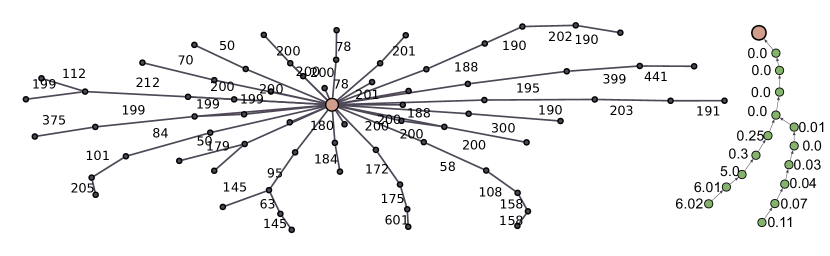
Figure 9. Short-term backward (ST-BK) paths for the instance address in the first $24$ hours (gray and green edges stand for ST-BK paths of the address’s first and second incoming transactions.). The numbers stand for the transaction volumes. The pink nodes are instance-related transactions.

7.7. Scalability Analysis

Generally speaking, users only want to monitor the new and large-volume addresses that have transactions with them. Those addresses are likely to participate in dangerous activities. Our system will dynamically monitor and update their transaction features every hour, as shown in Fig. 3(b). Then, the model proposes segments according to the default position and prepares the segment and status representations. In this way, our intention monitor can predict the labels dynamically.

In addition, to verify the model’s scalability, we randomly selected $1,000$ blocks (from the first block of $2020$ to the first block of $2022$) and collected the daily BTC price during this period. We filter out transactions lower than $$10,000$ and retrieve addresses with a lifespan smaller than one week. We got $299,767$ transactions and $181,221$ addresses. To get stronger proof of the model’s scalability, we fetch the data of the early $200$ hours (larger than one week) with a one-hour interval. The time costs under single-process and multi-process (acceleration by 20 processes) are illustrated as follows:

Table 5. Time cost of different input data, including block number, transaction number, address number), address feature, LT transfer path, and ST transfer path.

Block Number	Transaction Number	Address Number	Address Feature	LT-Path	ST-Path
1,000 (Single-Process)	299,767	181,221	0.51h	72.53h	130.33h
1,000 (Multi-Process)	299,767	181,221	0.03h	3.82h	6.86h
Avg (Multi-Process)	300	181	0.11s	13.75s	24.70s

On average, for the early $200$ hours, preparing an address feature takes $0.11$s. The LT and ST path feature take $13.75$s and $24.70$s, respectively. So we only need $2.42$s to prepare data in every one-hour interval.

8. Conclusion

This paper presents Intention Monitor, a novel framework for the early detection of malicious addresses on BTC. After proposing two kinds of asset transfer paths, we select, complement, and split the feature sequence for different malicious activities with a decision tree based strategy. In particular, we propose status and action vectors to describe the temporal behaviors and global semantic status and action. We build the Intention-VAE to propose intent-snippets and weight the contribution of status and action backbone predictions dynamically. A survival module based on Intention-VAE fine-tunes the weighted predictions and groups intent-snippets into the sequence of intention motif. We quantitatively and qualitatively evaluated the model on three malicious address datasets. Extensive ablation studies were conducted to determine the mechanisms behind the model’s effectiveness. The experimental results show that the proposed method outperformed the state-of-the-art baseline approaches on all three datasets. Furthermore, a detailed case study on Binance Hack justifies that our model can not only explain suspicious transaction patterns but can also find hidden abnormal signals.

9. Acknowledgments

This research is supported by the National Research Foundation Singapore under its Emerging Areas Research Projects (EARP) Funding Initiative, Industry Alignment Fund – Pre-positioning (IAF-PP) Funding Initiative, the NSFC (72171071, 72271084, 72101079), and the Excellent Fund of HFUT (JZ2021HGPA0060). Any opinions, findings and conclusions or recommendations expressed in this material are those of the author(s) and do not reflect the views of National Research Foundation, Singapore.

References

- (1)
- Abay et al. (2019) Nazmiye Ceren Abay, Cuneyt Gurcan Akcora, Yulia R Gel, Murat Kantarcioglu, Umar D Islambekov, Yahui Tian, and Bhavani Thuraisingham. 2019. Chainnet: Learning on blockchain graphs with topological features. In 2019 IEEE international conference on data mining (ICDM). IEEE, 946–951.
- Akcora et al. (2019) Cuneyt Gurcan Akcora, Yitao Li, Yulia R Gel, and Murat Kantarcioglu. 2019. BitcoinHeist: Topological data analysis for ransomware detection on the bitcoin blockchain. arXiv preprint arXiv:1906.07852 (2019).
- Al Jawaheri et al. (2020) Husam Al Jawaheri, Mashael Al Sabah, Yazan Boshmaf, and Aiman Erbad. 2020. Deanonymizing Tor hidden service users through Bitcoin transactions analysis. Computers & Security 89 (2020), 101684.
- Androulaki et al. (2013) Elli Androulaki, Ghassan O Karame, Marc Roeschlin, Tobias Scherer, and Srdjan Capkun. 2013. Evaluating user privacy in bitcoin. In International conference on financial cryptography and data security. Springer, 34–51.
- Aziz et al. (2022) Rabia Musheer Aziz, Mohammed Farhan Baluch, Sarthak Patel, and Abdul Hamid Ganie. 2022. LGBM: a machine learning approach for Ethereum fraud detection. International Journal of Information Technology (2022), 1–11.
- Bartoletti et al. (2018) Massimo Bartoletti, Barbara Pes, and Sergio Serusi. 2018. Data mining for detecting bitcoin ponzi schemes. In 2018 Crypto Valley Conference on Blockchain Technology (CVCBT). IEEE, 75–84.
- Bryans (2014) Danton Bryans. 2014. Bitcoin and money laundering: mining for an effective solution. Ind. LJ 89 (2014), 441.
- Chen et al. (2020b) Huashan Chen, Marcus Pendleton, Laurent Njilla, and Shouhuai Xu. 2020b. A survey on ethereum systems security: Vulnerabilities, attacks, and defenses. ACM Computing Surveys (CSUR) 53, 3 (2020), 1–43.
- Chen et al. (2020c) Liang Chen, Jiaying Peng, Yang Liu, Jintang Li, Fenfang Xie, and Zibin Zheng. 2020c. Phishing scams detection in ethereum transaction network. ACM Transactions on Internet Technology (TOIT) 21, 1 (2020), 1–16.
- Chen et al. (2020a) Ting Chen, Zihao Li, Yuxiao Zhu, Jiachi Chen, Xiapu Luo, John Chi-Shing Lui, Xiaodong Lin, and Xiaosong Zhang. 2020a. Understanding ethereum via graph analysis. ACM Transactions on Internet Technology (TOIT) 20, 2 (2020), 1–32.
- Chen et al. (2018) Weili Chen, Zibin Zheng, Jiahui Cui, Edith Ngai, Peilin Zheng, and Yuren Zhou. 2018. Detecting ponzi schemes on ethereum: Towards healthier blockchain technology. In Proceedings of the 2018 world wide web conference. 1409–1418.
- Chen et al. (2019) Weili Chen, Zibin Zheng, Edith C-H Ngai, Peilin Zheng, and Yuren Zhou. 2019. Exploiting blockchain data to detect smart ponzi schemes on ethereum. IEEE Access 7 (2019), 37575–37586.
- Cho et al. (2014) Kyunghyun Cho, Bart van Merriënboer, Dzmitry Bahdanau, and Yoshua Bengio. 2014. On the Properties of Neural Machine Translation: Encoder–Decoder Approaches. In Proceedings of SSST-8, Eighth Workshop on Syntax, Semantics and Structure in Statistical Translation. 103–111.
- Connolly and Wall (2019) Lena Y Connolly and David S Wall. 2019. The rise of crypto-ransomware in a changing cybercrime landscape: Taxonomising countermeasures. Computers & Security 87 (2019), 101568.
- Conti et al. (2018) Mauro Conti, Ankit Gangwal, and Sushmita Ruj. 2018. On the economic significance of ransomware campaigns: A Bitcoin transactions perspective. Computers & Security 79 (2018), 162–189.
- Fanusie and Robinson (2018) Yaya Fanusie and Tom Robinson. 2018. Bitcoin laundering: an analysis of illicit flows into digital currency services. Center on Sanctions and Illicit Finance memorandum, January (2018).
- Fleder et al. (2015) Michael Fleder, Michael S Kester, and Sudeep Pillai. 2015. Bitcoin transaction graph analysis. arXiv preprint arXiv:1502.01657 (2015).
- Foley et al. (2019) Sean Foley, Jonathan R Karlsen, and Tālis J Putniņš. 2019. Sex, drugs, and bitcoin: How much illegal activity is financed through cryptocurrencies? The Review of Financial Studies 32, 5 (2019), 1798–1853.
- Francesco Maesa et al. (2016) Damiano Di Francesco Maesa, Andrea Marino, and Laura Ricci. 2016. An analysis of the Bitcoin users graph: inferring unusual behaviours. In International Workshop on Complex Networks and their Applications. Springer, 749–760.
- Harlev et al. (2018) Mikkel Alexander Harlev, Haohua Sun Yin, Klaus Christian Langenheldt, Raghava Mukkamala, and Ravi Vatrapu. 2018. Breaking bad: De-anonymising entity types on the bitcoin blockchain using supervised machine learning. In Proceedings of the 51st Hawaii international conference on system sciences.
- Jaskie and Spanias (2019) Kristen Jaskie and Andreas Spanias. 2019. Positive and unlabeled learning algorithms and applications: A survey. In 2019 10th IISA. IEEE, 1–8.
- Kingma and Welling (2013) Diederik P Kingma and Max Welling. 2013. Auto-encoding variational bayes. arXiv preprint arXiv:1312.6114 (2013).
- Klusman and Dijkhuizen (2018) Robin Klusman and Tim Dijkhuizen. 2018. Deanonymisation in ethereum using existing methods for bitcoin.
- Li et al. (2019) Ji Li, Chunxiang Gu, Fushan Wei, and Xi Chen. 2019. A survey on blockchain anomaly detection using data mining techniques. In International Conference on Blockchain and Trustworthy Systems. Springer, 491–504.
- Li et al. (2022) Sijia Li, Gaopeng Gou, Chang Liu, Chengshang Hou, Zhenzhen Li, and Gang Xiong. 2022. TTAGN: Temporal Transaction Aggregation Graph Network for Ethereum Phishing Scams Detection. In Proceedings of the ACM Web Conference 2022. 661–669.
- Li et al. (2020) Yang Li, Yue Cai, Hao Tian, Gengsheng Xue, and Zibin Zheng. 2020. Identifying illicit addresses in bitcoin network. In International Conference on Blockchain and Trustworthy Systems. Springer, 99–111.
- Liang et al. (2019) Jiaqi Liang, Linjing Li, Shu Luan, Lu Gan, and Daniel Zeng. 2019. Bitcoin exchange addresses identification and its application in online drug trading regulation. In 23rd Pacific Asia Conference on Information Systems: Secure ICT Platform for the 4th Industrial Revolution, PACIS 2019.
- Lin et al. (2020a) Dan Lin, Jiajing Wu, Qi Yuan, and Zibin Zheng. 2020a. Modeling and understanding ethereum transaction records via a complex network approach. IEEE Transactions on Circuits and Systems II: Express Briefs 67, 11 (2020), 2737–2741.
- Lin et al. (2020b) Dan Lin, Jiajing Wu, Qi Yuan, and Zibin Zheng. 2020b. T-edge: Temporal weighted multidigraph embedding for ethereum transaction network analysis. Frontiers in Physics 8 (2020), 204.
- Liu et al. (2003) Bing Liu, Yang Dai, Xiaoli Li, Wee Sun Lee, and Philip S Yu. 2003. Building text classifiers using positive and unlabeled examples. In Third IEEE International Conference on Data Mining. IEEE, 179–186.
- Liu et al. (2021b) Can Liu, Li Sun, Xiang Ao, Jinghua Feng, Qing He, and Hao Yang. 2021b. Intention-aware heterogeneous graph attention networks for fraud transactions detection. In Proceedings of the 27th ACM SIGKDD Conference on Knowledge Discovery & Data Mining. 3280–3288.
- Liu et al. (2020) Can Liu, Qiwei Zhong, Xiang Ao, Li Sun, Wangli Lin, Jinghua Feng, Qing He, and Jiayu Tang. 2020. Fraud transactions detection via behavior tree with local intention calibration. In Proceedings of the 26th ACM SIGKDD International Conference on Knowledge Discovery & Data Mining. 3035–3043.
- Liu et al. (2021a) Yang Liu, Xiang Ao, Zidi Qin, Jianfeng Chi, Jinghua Feng, Hao Yang, and Qing He. 2021a. Pick and Choose: A GNN-Based Imbalanced Learning Approach for Fraud Detection. In Proceedings of the Web Conference 2021.
- McGinn et al. (2016) Dan McGinn, David Birch, David Akroyd, Miguel Molina-Solana, Yike Guo, and William J Knottenbelt. 2016. Visualizing dynamic bitcoin transaction patterns. Big data 4, 2 (2016), 109–119.
- McGinn et al. (2018) Dan McGinn, Doug McIlwraith, and Yike Guo. 2018. Towards open data blockchain analytics: a Bitcoin perspective. Royal Society open science 5, 8 (2018), 180298.
- Monaco (2015) John V Monaco. 2015. Identifying bitcoin users by transaction behavior. In Biometric and surveillance technology for human and activity identification XII, Vol. 9457. SPIE, 25–39.
- Möser et al. (2013) Malte Möser, Rainer Böhme, and Dominic Breuker. 2013. An inquiry into money laundering tools in the Bitcoin ecosystem. In 2013 APWG eCrime researchers summit. IEEE, 1–14.
- Möser et al. (2014) Malte Möser, Rainer Böhme, and Dominic Breuker. 2014. Towards risk scoring of Bitcoin transactions. In International conference on financial cryptography and data security. Springer, 16–32.
- Nerurkar et al. (2020) Pranav Nerurkar, Yann Busnel, Romaric Ludinard, Kunjal Shah, Sunil Bhirud, and Dhiren Patel. 2020. Detecting illicit entities in bitcoin using supervised learning of ensemble decision trees. In Proceedings of the 2020 10th international conference on information communication and management. 25–30.
- Paquet-Clouston et al. (2019) Masarah Paquet-Clouston, Bernhard Haslhofer, and Benoit Dupont. 2019. Ransomware payments in the bitcoin ecosystem. Journal of Cybersecurity 5, 1 (2019), tyz003.
- Pham and Lee (2016) Thai Pham and Steven Lee. 2016. Anomaly detection in the bitcoin system-a network perspective. arXiv preprint arXiv:1611.03942 (2016).
- Prado-Romero et al. (2017) Mario Alfonso Prado-Romero, Christian Doerr, and Andrés Gago-Alonso. 2017. Discovering bitcoin mixing using anomaly detection. In Iberoamerican Congress on Pattern Recognition. Springer, 534–541.
- Ranshous et al. (2017) Stephen Ranshous, Cliff A Joslyn, Sean Kreyling, Kathleen Nowak, Nagiza F Samatova, Curtis L West, and Samuel Winters. 2017. Exchange pattern mining in the bitcoin transaction directed hypergraph. In International conference on financial cryptography and data security. Springer, 248–263.
- Reid and Harrigan (2013) Fergal Reid and Martin Harrigan. 2013. An analysis of anonymity in the bitcoin system. In Security and privacy in social networks. Springer, 197–223.
- Shao et al. (2018) Wei Shao, Hang Li, Mengqi Chen, Chunfu Jia, Chunbo Liu, and Zhi Wang. 2018. Identifying bitcoin users using deep neural network. In International Conference on Algorithms and Architectures for Parallel Processing. Springer, 178–192.
- Song et al. (2021) Chenguang Song, Nianwen Ning, Yunlei Zhang, and Bin Wu. 2021. Knowledge augmented transformer for adversarial multidomain multiclassification multimodal fake news detection. Neurocomputing 462 (2021), 88–100.
- Song et al. (2019) Changhe Song, Cheng Yang, Huimin Chen, Cunchao Tu, Zhiyuan Liu, and Maosong Sun. 2019. CED: Credible early detection of social media rumors. IEEE Transactions on Knowledge and Data Engineering (2019).
- Sun et al. (2012) Yizhou Sun, Jiawei Han, Charu C. Aggarwal, and Nitesh V. Chawla. 2012. When Will It Happen? Relationship Prediction in Heterogeneous Information Networks. In Proceedings of the Fifth ACM International Conference on Web Search and Data Mining (WSDM ’12). 663–672. https://doi.org/10.1145/2124295.2124373
- Tam et al. (2019) Da Sun Handason Tam, Wing Cheong Lau, Bin Hu, Qiu Fang Ying, Dah Ming Chiu, and Hong Liu. 2019. Identifying Illicit Accounts in Large Scale E-payment Networks–A Graph Representation Learning Approach. arXiv preprint arXiv:1906.05546 (2019).
- Vasek and Moore (2015) Marie Vasek and Tyler Moore. 2015. There’s no free lunch, even using Bitcoin: Tracking the popularity and profits of virtual currency scams. In International conference on financial cryptography and data security. Springer, 44–61.
- Weber et al. (2019) Mark Weber, Giacomo Domeniconi, Jie Chen, Daniel Karl I Weidele, Claudio Bellei, Tom Robinson, and Charles E Leiserson. 2019. Anti-money laundering in bitcoin: Experimenting with graph convolutional networks for financial forensics. arXiv preprint arXiv:1908.02591 (2019).
- Wu et al. (2021) Jiajing Wu, Jieli Liu, Weili Chen, Huawei Huang, Zibin Zheng, and Yan Zhang. 2021. Detecting mixing services via mining bitcoin transaction network with hybrid motifs. IEEE Transactions on Systems, Man, and Cybernetics: Systems (2021).
- Wu et al. (2020) Jiajing Wu, Qi Yuan, Dan Lin, Wei You, Weili Chen, Chuan Chen, and Zibin Zheng. 2020. Who are the phishers? phishing scam detection on ethereum via network embedding. IEEE Transactions on Systems, Man, and Cybernetics: Systems (2020).
- Wu et al. (2018) Zhiang Wu, Jie Cao, Yaqiong Wang, Youquan Wang, Lu Zhang, and Junjie Wu. 2018. hPSD: a hybrid PU-learning-based spammer detection model for product reviews. IEEE transactions on cybernetics 50, 4 (2018), 1595–1606.
- Yin and Vatrapu (2017) Haohua Sun Yin and Ravi Vatrapu. 2017. A first estimation of the proportion of cybercriminal entities in the bitcoin ecosystem using supervised machine learning. In 2017 IEEE International Conference on Big Data (Big Data). IEEE, 3690–3699.
- Yuan et al. (2017) Shuhan Yuan, Panpan Zheng, Xintao Wu, and Yang Xiang. 2017. Wikipedia vandal early detection: from user behavior to user embedding. In Joint European Conference on Machine Learning and Knowledge Discovery in Databases. Springer, 832–846.
- Zheng et al. (2019) Panpan Zheng, Shuhan Yuan, and Xintao Wu. 2019. Safe: A neural survival analysis model for fraud early detection. In Proceedings of the AAAI Conference on Artificial Intelligence, Vol. 33. 1278–1285.
- Zola et al. (2019) Francesco Zola, Jan Lukas Bruse, Maria Eguimendia, Mikel Galar, and Raul Orduna Urrutia. 2019. Bitcoin and cybersecurity: Temporal dissection of blockchain data to unveil changes in entity behavioral patterns. Applied Sciences 9, 23 (2019), 5003.