From Peptides to Nanostructures: A Euclidean Transformer for
Fast and Stable Machine Learned Force Fields

Abstract

Recent years have seen vast progress in the development of machine learned force fields (MLFFs) based on ab-initio reference calculations. Despite achieving low test errors, the suitability of MLFFs in molecular dynamics (MD) simulations is being increasingly scrutinized due to concerns about instability. Our findings suggest a potential connection between MD simulation stability and the presence of equivariant representations in MLFFs, but their computational cost can limit practical advantages they would otherwise bring.

To address this, we propose a transformer architecture called SO3krates that combines sparse equivariant representations (Euclidean variables) with a self-attention mechanism that can separate invariant and equivariant information, eliminating the need for expensive tensor products. SO3krates achieves a unique combination of accuracy, stability, and speed that enables insightful analysis of quantum properties of matter on unprecedented time and system size scales. To showcase this capability, we generate stable MD trajectories for flexible peptides and supra-molecular structures with hundreds of atoms. Furthermore, we investigate the PES topology for medium-sized chainlike molecules (e.g., small peptides) by exploring thousands of minima. Remarkably, SO3krates demonstrates the ability to strike a balance between the conflicting demands of stability and the emergence of new minimum-energy conformations beyond the training data, which is crucial for realistic exploration tasks in the field of biochemistry.

I Introduction

Atomistic modeling relies on long-timescale molecular dynamics (MD) simulations to reveal how experimentally observed macroscopic properties of a system emerge from interactions on the microscopic scale [1]. The predictive accuracy of such simulations is determined by the accuracy of the interatomic forces that drive them. Traditionally, these forces are either obtained from exceedingly approximate mechanistic force fields (FF) or accurate, but computationally prohibitive ab initio electronic structure calculations. Recently, machine learning (ML) potentials have started to bridge this gap, by exploiting statistical dependencies of molecular systems with so far unprecedented flexibility [2, 3, 4, 5, 6, 7, 8, 9, 10, 11, 12, 13, 14, 15, 16, 17, 18, 19, 20, 21, 22, 23, 24, 25].

The accuracy of MLFFs is traditionally determined by their test errors on a few established benchmark datasets [8, 26, 27]. Despite providing an initial estimate of MLFF accuracy, recent research [28, 29, 30] indicates that there is only a weak correlation between MLFF test errors and their performance in long MD simulations, which is considered the true measure of predictive usefulness. Faithful representations of dynamical and thermodynamic observables can only be derived from accurate MD trajectories. From an ML perspective this shortcoming can be attributed to poor extrapolation behavior, which becomes particularly severe for high temperature configurations or conformationally flexible structures. In these cases, the geometries explored during MD simulations significantly deviate from the distribution of the training data.

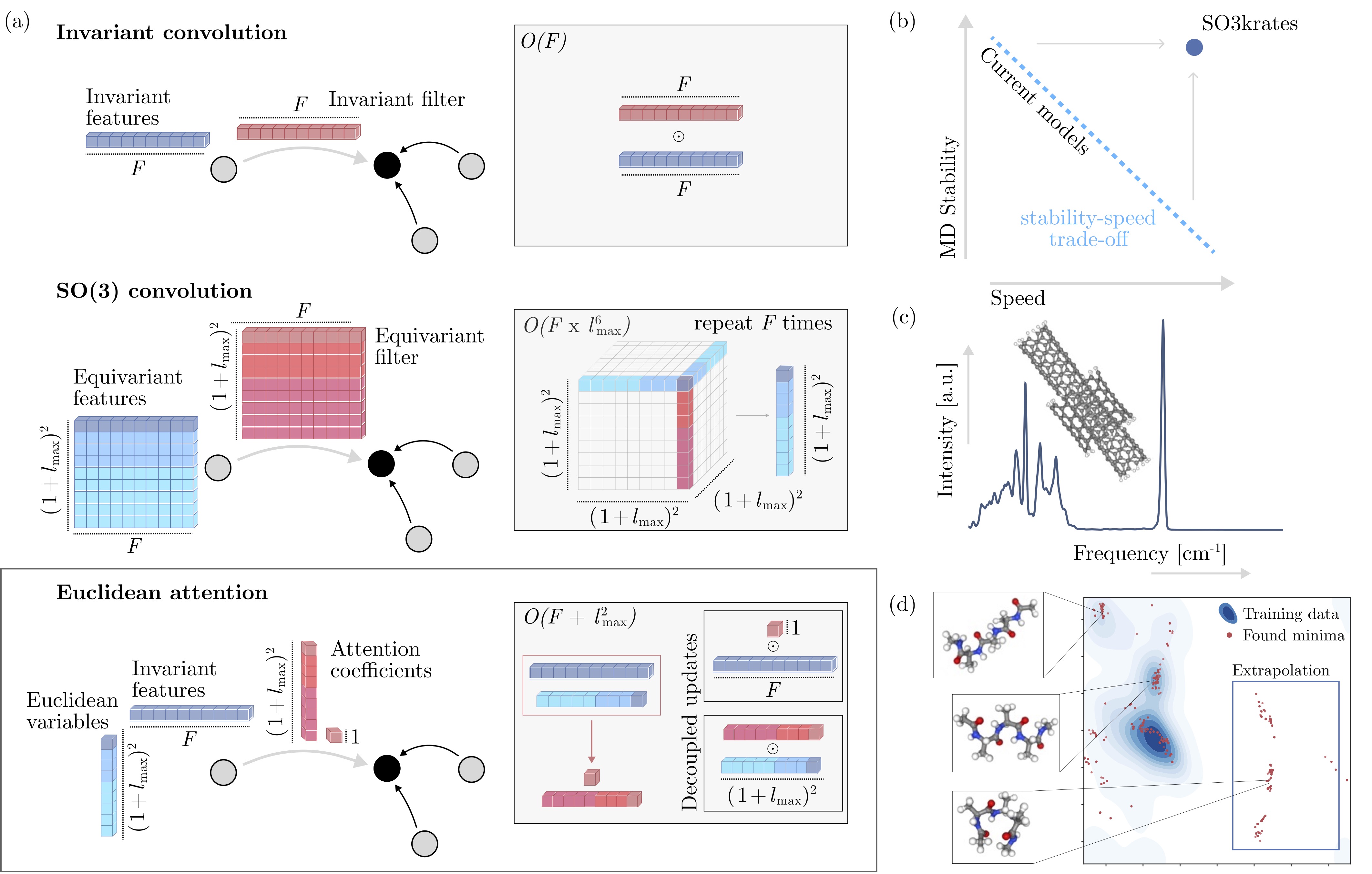
Figure 1: (a) Illustration of an invariant convolution, an SO(3) convolution and of the Euclidean attention mechanism that underlies the SO3krates transformer. We decompose the representation of molecular structure into high dimensional invariant features and equivariant Euclidean variables (EV), which interact via self-attention. (b) The proposed design paradigm can help to overcome current trade-offs between stability in MD simulations and computational efficiency experienced for other (equivariant) MPNNs. (c) Computational efficiency of SO3krates allows the calculation of velocity-auto correlation functions from converged MD simulations for supra-molecular structures. (d) SO3krates enables to explore thousands of minima of the potential energy surface of small chainlike molecules such as Ac-Ala3-NHMe or DHA, where SO3krates can robustly extrapolate beyond the training data.

The ongoing progress in MLFF development has resulted in a wide range of increasingly sophisticated model architectures aiming to improve the extrapolation behavior. Among these, message passing neural networks (MPNNs) [9, 31, 12] have emerged as a particularly effective class of architectures. MPNNs can be considered as a generalization of convolutions to handle unstructured data domains, such as molecular graphs. This operation provides an effective way to extract features from the input data and is ubiquitous in many modern ML architectures. Recent advances in this area focused on the incorporation of physically meaningful geometric priors [8, 11, 32, 23, 33]. This has lead to so-called equivariant MPNNs, which have been found to reduce the obtained approximation error [34, 33, 35, 36] and offer better data efficiencies than invariant models [33]. Invariant models rely on pairwise distances to describe atomic interactions, as they do not change upon rotation [5]. However, with growing system size, flexibility or chemical heterogeneity, it becomes increasingly harder to derive the correct interaction patterns within this limited representation. This is why equivariant models enable to incorporate additional directional information, to capture interactions depending on the relative orientation of neighboring atoms. It allows them to discriminate interactions that can appear inseparable to simpler models [34] and to learn more transferable interaction patterns from the same training data.

A fundamental building block of most equivariant architectures is the tensor product. It is evaluated within the convolution operation $(f*g)(x)$ between pairs of functions $f(x)$ and $g(x)$ expanded in linear bases [37]. The result is then defined in the product space of the original basis function sets. Thus, the associated product space quickly becomes computationally intractable as it grows exponentially in the number of convolution operations.

In SO(3) equivariant architectures, convolutions are performed over the SO(3) group of rotations in the basis of the spherical harmonics. By doing so, the exponential growth of the associated function space can be avoided by fixing the maximum degree $l_{\mathrm{max}}$ of the spherical harmonics in the architecture. The largest degree has been shown to be closely connected to accuracy, data efficiency [24, 33] and offer the potential for more reliable MD simulations. However, SO(3) convolutions scale as $l_{\mathrm{max}}^{6}$, which can increase the prediction time per conformation by up to two orders of magnitude compared to an invariant model [38, 30]. This has lead to a situation where one has to compromise between accuracy, stability and speed, which can pose significant practical problems that need to be addressed before such models can become useful in practice for high-throughput or extensive exploration tasks.

Architecture	Scaling	$l_{\mathrm{max}}$
SchNet [9]	$\mathcal{O}(n\times\braket{\mathcal{N}}\times F)$	0
PaiNN [34]	$\mathcal{O}(n\times\braket{\mathcal{N}}\times l_{\mathrm{max}}^{2}\times F)$	1
SpookyNet [24]	$\mathcal{O}(n\times\braket{\mathcal{N}}\times l_{\mathrm{max}}^{2}\times F)$	2
NequIP [33]	$\mathcal{O}(n\times\braket{\mathcal{N}}\times l_{\mathrm{max}}^{6}\times F)$	3
SO3krates	$\mathcal{O}(n\times\braket{\mathcal{N}}\times(l_{\mathrm{max}}^{2}+F))$	3

Table 1: Scaling for different (equivariant) message passing architectures, where $n$ is the number of atoms, $\braket{\mathcal{N}}$ the average number of neighbors and $l_{\mathrm{max}}$ the maximal degree.

We take this as motivation to propose an Euclidean self-attention mechanism that replaces SO(3) convolutions with a filter on the relative orientation of atomic neighborhoods, representing atomic interactions without the need for expensive tensor products. Our solution builds on recent advances in neural network architecture design [39] and from the field of geometric deep learning [40, 34, 33, 35]. Our SO3krates method uses a sparse representation for the molecular geometry and restricts projections of all convolution responses to the most relevant invariant component of the equivariant basis functions. Due to the orthonormality of the spherical harmonics, such a projection corresponds to partial traces of the product-tensor, which can be expressed in terms of linear-scaling inner products. This enables efficient scaling to high degree equivariant representations without sacrificing computational speed and memory cost. Force predictions are obtained from the gradient of the resulting invariant energy model, which represents a piece-wise linearization that is naturally equivariant. Throughout, a self-attention mechanism is used to decouple invariant and equivariant basis elements within the model.

We compare the stability and speed of the proposed SO3krates model with current state-of-the art ML potentials and find that our solution overcomes the limitations of current equivariant MLFFs, without compromising on their advantages. Our proposed mathematical formulation leading to an efficient equivariant architecture enables reliably stable MD simulations with a speedup of up to a factor of $\sim 25$ over equivariant MPNNs with comparable stability and accuracy [30].

To demonstrate this, we run accurate nanosecond-long MD simulations for supra-molecular structures within only a few hours, which allows us to calculate converged auto-correlation functions (vibrational spectra) for structures that range from small peptides with 42 atoms up to nanostructures with 370 atoms. We further apply our model to explore the topology of the PES of docosahexaenoic acid (DHA) and Ac-Ala3-NHMe by investigating 10k minima using a minima hopping algorithm [41]. Such an investigation requires roughly 30M FF evaluations that are queried at temperatures between a few 100 K up to $\sim\!1200$ K. With DFT methods, this analysis would require more than a year of computation time. Existing equivariant MLFFs with comparable prediction accuracy would run more than a month for such an analysis. In contrast, we are able to perform the simulation in only 2.5 days, opening up the possibility to explore hundreds of thousands of PES minima on practical timescales. In one of our experiments, we further show that SO3krates enables the detection of physically valid minima conformations which have not been part of the training data. The ability to extrapolate to unknown parts of the PES is essential for scaling MLFFs to large structures, since the availability of ab-initio reference data can only cover sub-regions for conformationally rich structures.

Figure 2: SO(3) convolutions are constructed as triplet tensor products in the spherical harmonics basis, which is performed $F$ times along the feature dimension. We replace SO(3) convolutions by a parametrized filter function on the invariants (red blocks), which effectively reduces the tripled tensor product to taking the partial (per-degree) trace of a simple tensor product. Colored volumes correspond to the non-zero entries in the Clebsch-Gordan coefficients, which mask the tensor products.

Furthermore, we examine the impact of disabling the equivariance property in our network architecture to gain a deeper understanding of its influence on the characteristics of the model and its reliability in MD simulations. We find, that the equivariant nature can be linked to the stability of the resulting MD simulation and to the extrapolation behavior to higher temperatures. We are able to show, that equivariance lowers the spread in the error distribution even when the test error estimate is the same on average. Thus, using directional information via equivariant representations shows analogies in spirit to classical ML theory, where mapping into higher dimensions yields richer features spaces that are easier to parametrize [42, 43, 44].

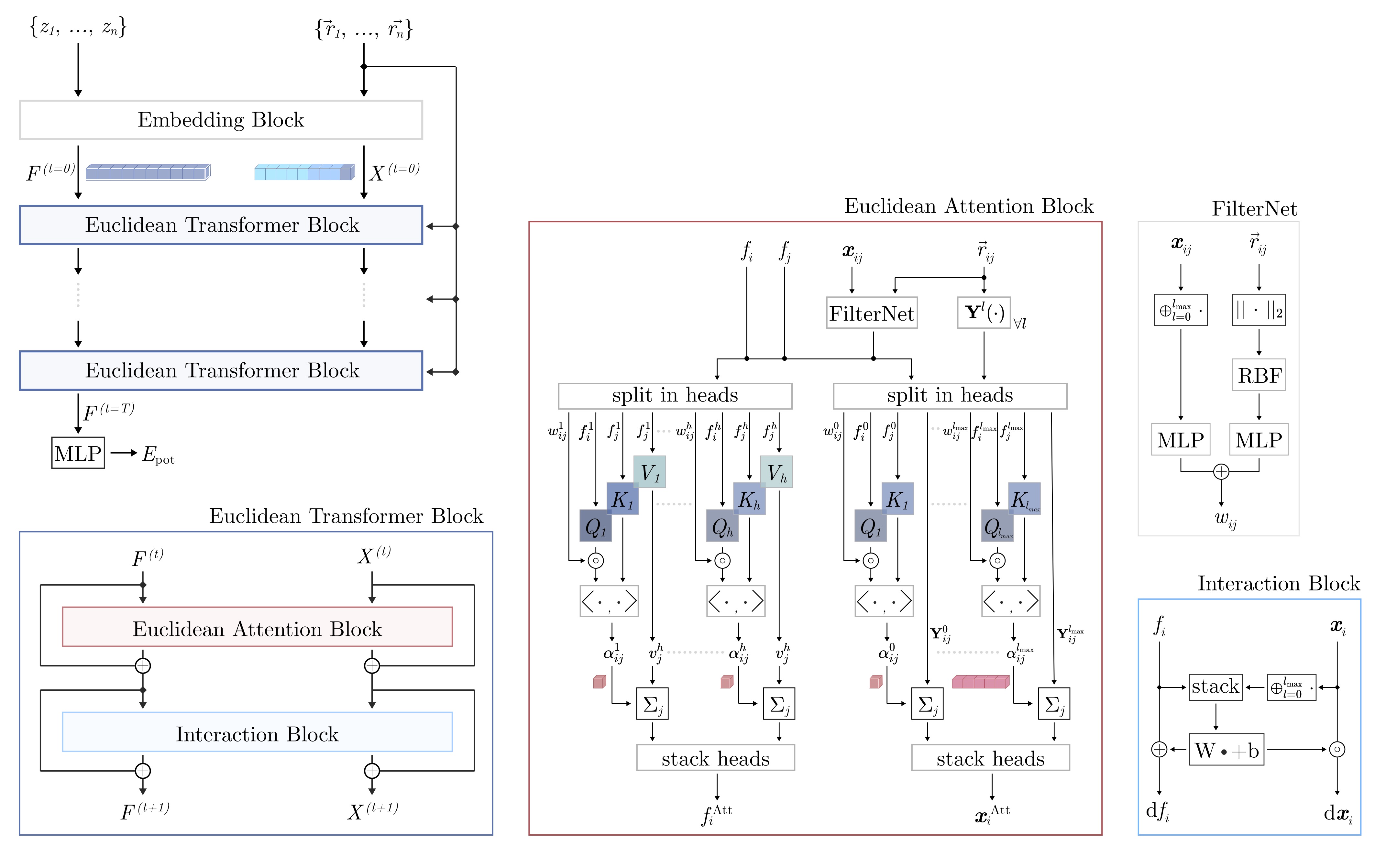
Figure 3: SO3krates architecture and building blocks. Taking the atomic types and positions as input they are embedded into invariant features $F$ and equivariant EV $X$ (methods section IV.1). They are then refined by $T$ Euclidean transformer blocks (ecTblock) (Eq. (9)) before the final invariant features are used to predict the potential energy (Eq. (1)). After the Euclidean attention block, features and EV exchange per-atom information within the interaction block. Both blocks are enveloped by skip connection which allows to carry over information from prior layers. For an in detail description of the individual parts see methods section.

II Results

II.1 From Equivariant Message Passing Neural Networks to Separating Invariant and Equivariant Structure: SO3krates

MPNNs [31] carry over many of the properties of convolutions to unstructured input domains, such as sets of atomic positions in Euclidean space. This has made them one promising approach for the description of the PES [12, 17, 45, 24, 33, 46, 47], where the potential energy is typically predicted as

$$E_{\text{pot}}(\vec{r}_{1},\dots,\vec{r}_{n})=\sum_{i=1}^{n}E_{i}.$$ (1)

The energy contributions $E_{i}\in\mathbb{R}$ are calculated from high dimensional atomic representations $f_{i}^{[T]}$. They are constructed iteratively (from $T$ steps), by aggregating pairwise messages $m_{ij}$ over atomic neighborhoods $\mathcal{N}(i)$

$$f_{i}^{[t+1]}=\textsc{Upd}\left(f_{i}^{[t]},\bigoplus_{j\in\mathcal{N}(i)}m_{ij}\right),$$ (2)

where $\textsc{Upd}(\cdot)$ is an update function that mixes the representations from the prior iteration and the aggregated messages.

One way of incorporating the rotational invariance of the PES is to build messages that are based on invariant inputs such as distances, angles or dihedral angles. However, this incomplete list of features can not discriminate certain interaction patterns [48]. An alternative is to use SO(3) equivariant representations [49, 33, 47, 35] within a basis that allows for systematic expansion to match the complexity of the modelled system.

This requires to generalize the concept of invariant continuous convolutions [12] to the SO(3) group of rotations. A message function performing an SO(3) convolution can be written as [37, 33]

$$m_{ij}^{LM}=\sum_{l_{1}l_{2}m_{1}m_{2}}C_{l_{1}l_{2}L}^{m_{1}m_{2}M}\phi^{l_{1}l_{2}L}(r_{ij})Y_{l_{1}}^{m_{1}}(\hat{r}_{ij})f_{j}^{l2m2},$$ (3)

where $C_{l_{1}l_{2}L}^{m_{1}m_{2}M}$ are the Clebsch-Gordan coefficients, $Y^{l}_{m}$ is a spherical harmonic of degree $l$ and order $m$, the function $\phi^{l_{1}l_{2}}:\mathbb{R}\mapsto\mathbb{R}^{F}$ modulates the radial part and $f_{j}^{l_{2}m_{2}}\in\mathbb{R}^{F}$ is an atomic feature vector. Thus, performing a single convolution scales as $\mathcal{O}(l_{\mathrm{max}}^{6}\times F)$, where $l_{\mathrm{max}}$ is the largest degree in the network (Fig. 2).

Here we propose two conceptual changes to Eq. (3) that we will denote as Euclidean self-attention: (1) We separate the message into an invariant and an equivariant part and (2) replace the SO(3) convolution by and attention function on its invariant output. To do so, we start by initializing atomic features $f_{i}^{[t=0]}\in\mathbb{R}^{F}$ and Euclidean variables (EV) $x_{i,LM}^{[t=0]}\in\mathbb{R}$ from the atomic types and the atomic neighborhoods, respectively. Collecting all orders and degrees for the EV in a single vector, gives $(l_{\mathrm{max}}+1)^{2}$ dimensional representations $\bm{x}_{i}$ that transform equivariant under rotation and capture directional information up to degree $l_{\mathrm{max}}$ (methods section IV.1).

(1) The message for the invariant part is written as

$$m_{ij}=\alpha_{ij}f_{j}$$ (4)

and the one for the equivariant part as

$$m_{ijLM}=\alpha_{ij,L}Y^{M}_{L}(\hat{r}_{ij}),$$ (5)

where $\alpha_{ij}\in\mathbb{R}$ are (per-degree) attention coefficients. Features and EV are updated with the aggregated messages, which writes as

$$f_{i}^{[t+1]}=f_{i}^{[t]}+\sum_{j\in\mathcal{N}(i)}m_{ij}$$ (6)

for the features and as

$$x_{iLM}^{[t+1]}=x_{iLM}^{[t]}+\sum_{j\in\mathcal{N}(i)}m_{ijLM}.$$ (7)

for the EV. Due to the separation, the overall message calculation scales as $\mathcal{O}(l_{\mathrm{max}}^{2}+F)$, replacing the multiplication of feature dimension and $l_{\mathrm{max}}$ from other equivariant architectures by addition (Tab. 1).

(2) Instead of performing full SO(3) convolutions, we move the learning of complex interaction patterns into an attention function

$$\alpha_{ij}=\alpha\left(f_{i},f_{j},r_{ij},\oplus_{l=0}^{l_{\mathrm{max}}}\bm{x}_{ij,l\shortrightarrow 0}\right),$$ (8)

where $\oplus_{l=0}^{l_{\mathrm{max}}}\bm{x}_{ij,l\shortrightarrow 0}$ is the invariant output of the SO(3) convolution over the EV signals located on atom $i$ and $j$ (methods section IV.2). Thus, Eq. (8) non-linearly incorporates information about the relative orientation of atomic neighborhoods. Since the Clebsch-Gordan coefficients are diagonal matrices along the $l=0$ axis (Fig. 2), calculating the invariant projections requires to take per-degree traces of length $(2l+1)$ and can be computed efficiently in $\mathcal{O}(l_{\mathrm{max}}^{2})$. Within SO3krates atomic representations are refined iteratively as

$$[\mathbf{f}_{i}^{[t+1]},\bm{x}_{i}^{[t+1]}\,]=\textsc{ecTblock}\big{[}\{\mathbf{f}_{j}^{[t]},\bm{x}_{j}^{[t]},\vec{r}_{ij}\}_{j\in\mathcal{N}(i)}\big{]},$$ (9)

where each Euclidean transformer block (ecTblock) consists of a self-attention block and an interaction block. The self-attention block, implements the Euclidean self-attention mechanism described in the former section. The interaction block gives additional freedom for parametrization by exchanging information between features and EV located at the same atom. After $T$ MP steps, per-atom energies $E_{i}$ are calculated from the final features $f_{i}^{[T]}$ using a two-layered neural network and are summed to the total potential energy (Eq. (1)). Atomic forces are obtained using automatic differentiation, which ensures energy conservation. A detailed outline of the architectural components and the proposed Euclidean self-attention framework is given in the methods section.

II.2 Overcoming Accuracy-Stability-Speed Trade-Offs

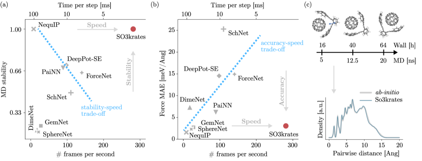
Figure 4: (a) Number of frames per second (FPS) vs. the averaged stability coefficient (Eq. (28)) in MD simulations run with different state-of-the-art MPNN architectures [33, 12, 34, 50, 38, 45, 51, 52] and (b) FPS vs. the averaged force MAE for four small organic molecules from the MD17 data set as reported in [30]. SO3krates yields reliable MD simulations and high accuracies without sacrificing computational performance. (c) Stability and speed of SO3krates enable nanosecond long MD simulations for supra molecular structures within a few hours. For the buckyball catcher, the ball stays in the catcher over the full simulation time of 20 ns, illustrating that the model successfully picks up on weak, non-covalent bonding.

We show in the following experiment, that SO3krates can overcome the trade-offs between MD stability, accuracy and computational efficiency (Fig. 4).

A recent study compared the stability of different state-of-the-art MLFFs in short MD simulations and found that only the SO(3) convolution based architecture NequIP [33] gave reliably stable results [30]. The excellent stability of such models, however, comes at the price of extensive computational cost (Fig. 4 (a)) which stems from equivariant features and SO(3) convolutions. This leads to a trade-off between the stability and the computational efficiency of MP based MLFFs, but SO3krates can overcome this stability-speed trade-off. It allows to predict up to one order of magnitude more frames per second (FPS) without sacrificing reliability in MD simulations. Although the test accuracy does not necessarily correlate with the stability (compare e.g. GemNet and SphereNet in Fig. 4 (a) and (b)), only accurate and stable models are of ultimate interest. We find, that SO3krates yields accurate force predictions, thus overcoming the complementary trade-off between accuracy and speed (Fig. 4 (b)).

For the radial distribution functions (RDFs), we find consistent results across five simulations (SI Fig. 12) for all of the four investigated structures, which are in agreement with the RDFs from DFT calculations. Interestingly, it has been found that other approaches with a larger number of FPS can give inaccurate RDFs, which result in MAEs between 0.35 for salicylic acid and 1.02 for naphthalene [30]. In comparison the achieved accuracies with SO3krates show that the seemingly contradictory requirements of high computational speed and accurate observables from MD trajectories can be reconciled.

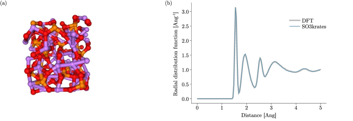
Figure 15: (a) Li₃PO₄ structure in the quenched phase. The shown conformation corresponds to the starting conformation for the MD simulation with SO3krates. (b) Radial distribution function obtained from the last 20ps of a 50 ps MD simulation at 600 K, compared to the RDF from DFT.

A recent work, proposed a strictly local equivariant architecture, called Allegro [53]. This allows for parallelization without additional communication, whereas parallelization of MPNNs with $T$ layers requires $T-1$ additional communication calls between computational nodes. On the example of the Li₃PO₄ solid electrolyte we compare accuracy and speed to the Allegro model for a unit cell with 192 atoms (Tab. 2). Remarkably, SO3krates achieves energy and force accuracies, more than 50% better than the ones reported in [53], even with only one tenth of the training data. At the same time, the timings in MD simulations are on par. To validate the physical validity of the obtained MD trajectory, we compare the RDFs at 600K to the ones obtained from DFT in the quenched phase of Li₃SO₄ (SI Fig. 15).

	$n_{\text{train}}$	$E_{\text{MAE}}$ [$\frac{\text{meV}}{\text{atom}}$]	$F_{\text{MAE}}$ [$\frac{\text{meV}}{$\mathrm{\SIUnitSymbolAngstrom}$}$]	$\frac{\mu\text{s}}{\text{step}\cdot\text{atom}}$
Allegro [53]	10k	1.7	73.4	27.785∗
SO3krates	10k	0.2	28.2	23.593∗
SO3krates	1k	0.3	31.8	23.593∗

Table 2: Speed in MD simulation and accuracy comparison to the strictly local Allegro model for Li₃PO₄ (192 atoms) on a single V100 GPU as reported in [53].

II.3 Data Efficiency, Stability and Extrapolation

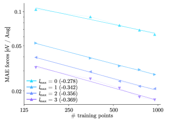
Figure 13: Figure shows the data efficiency measured in terms of force approximation error for the DHA molecule for different maximal degree $l_{\mathrm{max}}$ in the SO3krates network. With increasing $l_{\mathrm{max}}$, we find increasing data efficiency, which is calculated as the slope in the log-log plot, following [33]. The largest difference for both, accuracy and data efficiency can be found when going from an invariant ($l_{\mathrm{max}}=0$) to an equivariant model ($l_{\mathrm{max}}>0$).

Data efficiency and MD stability play an important role for the applicability of a MLFFs. High data efficiency allows to obtain accurate PES approximations even when only little data is available, which is a common setting due to the computational complexity of quantum mechanical ab-initio methods. Even when high accuracies can be achieved, without MD stability the calculation of physical observables from the trajectories becomes impossible. Here, we show that the data efficiency of SO3krates can be successively increased further by increasing the largest degree $l_{\mathrm{max}}$ in the network (SI Fig. 13). We further find, that the stability and extrapolation to higher temperatures of the MLFF can be linked to the presence of equivariant representations, independent of the test error estimate (Fig. 5).

To understand the benefits of directional information, we use an equivariant ($l_{\mathrm{max}}=3$) and an invariant model ($l_{\mathrm{max}}=0$) within our analysis. Due to the use of multi-head attention, the change in the number of network parameters is negligible when going from $l_{\mathrm{max}}=0$ to $l_{\mathrm{max}}=3$ (methods section IV.8). All models were trained on 11k randomly sampled geometries from which 1k are used for validation. This number of training samples was necessary to attain force errors close to 1 kcal mol^-1 $$\mathrm{\SIUnitSymbolAngstrom}$^{-1}$ for the invariant model. Since equivariant representations increase the data efficiency of ML potentials [33, 24], we expect the equivariant model to have a smaller test error estimate given the same number of training samples. We confirm this expectation on the example of the DHA molecule, where we compare the data efficiency for different degrees $l_{\mathrm{max}}$ on the example of the DHA molecule (SI Fig. 13).

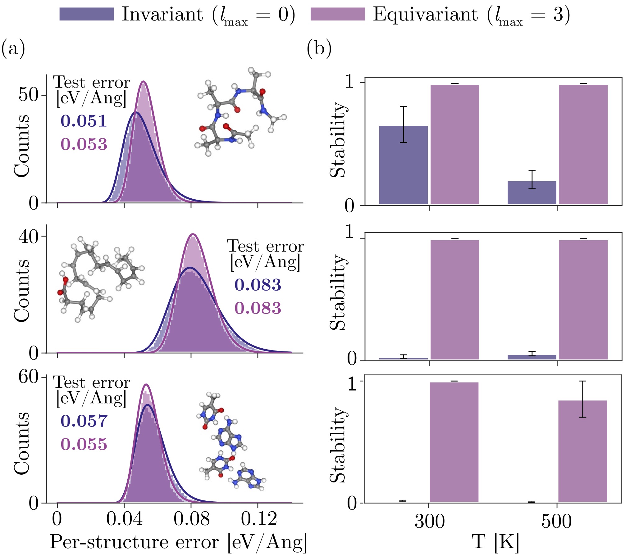
Figure 5: (a) Per-structure error distributions for an invariant and an equivariant SO3krates model with the same mean error on the test set. Spread and mean of the error distributions are given in SI Tab. 4. (b) The MD stability observed at temperatures 300 K and 500 K. The transition to higher temperatures results in a drop of stability for the invariant model, hinting towards less robustness and weaker extrapolation behavior. Flexible molecules such as DHA pose a challenge for the invariant model at 300 K already.

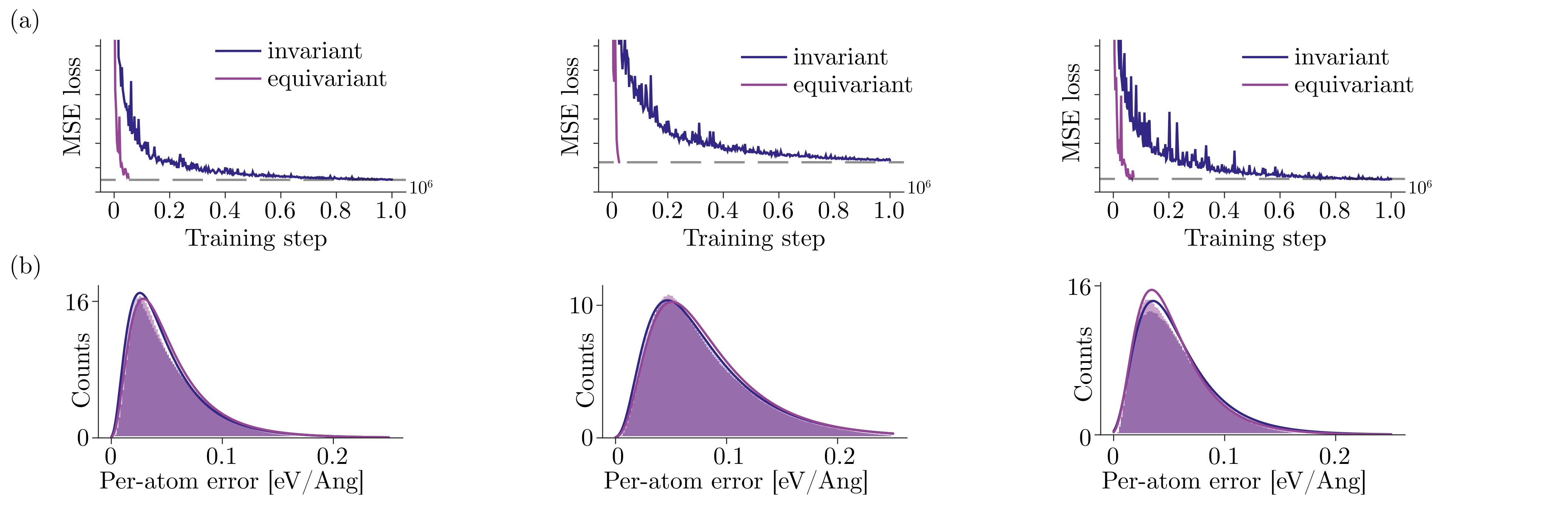
Figure 14: Plots from left to the right correspond to the structures Ac-Ala3-NHMe, DHA and the Adenine-Thymine pair (AT-AT). (a) Validation loss for an invariant ($l_{\mathrm{max}}=0$) and an equivariant ($l_{\mathrm{max}}=3$) SO3krates model observed during training, where the training of the equivariant model is stopped as soon as it reaches the error of the invariant model. (a) Per-atom error distributions for an invariant and an equivariant SO3krates model. Spread and mean of the error distributions are given in SI Tab. 4.

To make the comparison of invariant and equivariant model as fair as possible, we train the invariant model until the validation loss converges. Afterwards, we train the equivariant model towards the same validation error, which leads to identical errors on the unseen test set (Fig. 5 and SI Tab. 4). Since the equivariant model makes more efficient use of the training data, it requires only $\sim\nicefrac{{1}}{{5}}$ of the number of training steps of an invariant model to reach the same validation error (SI Fig. 14 (a)).

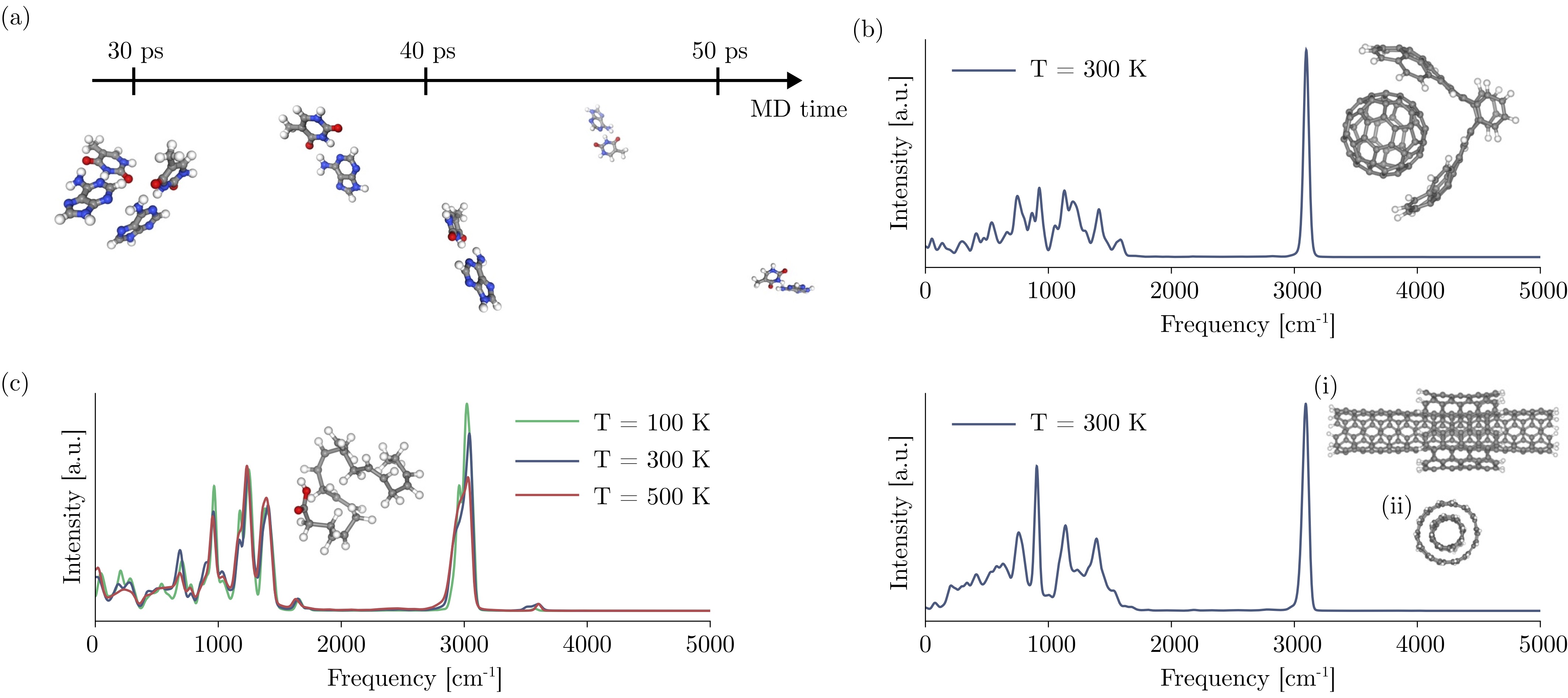
Figure 6: (a) Dissociation of the AT-AT complex over time, due to the breaking of $\pi$-$\pi$ interactions. (b) Velocity auto-correlation function for the buckyball catcher (upper) and the double-walled nanotube (lower). For the nanotube, the structure is shown from the side (i) and from the front (ii). (c) Temperature dependency of the velocity auto-correlation function, investigated along the DHA molecule for three different temperatures. All auto-correlation functions have been obtained from MD simulations over 1 ns.

After training, we compare the test error distributions since identical mean statistics do not imply a similar distribution. We calculate per atom force errors as $\epsilon_{i}=||\vec{F}_{i}-\vec{F}_{i}^{\text{GT}}||_{2}$ and compare the resulting distribution of the invariant and the equivariant model. The so observed distributions are identical in nature and only differ slightly in height and spread without the presence of a clear trend (SI Fig. 14 (b)). In the distributions of the per-structure $\mathcal{S}$ force error $R_{i}=\frac{1}{|\mathcal{S}|}\sum_{i\in\mathcal{S}}\epsilon_{i}$, however, one finds a consistently larger spread of the error (Fig. 5 (a)). Thus, the invariant model performs particularly well (and even better than the equivariant model) on certain conformations which comes at the price of worse performance for other conformations, a fact which is invisible to per-atom errors.

The stability coefficients (Eq. (28)) are determined from six 300 ps MD simulations with a time step of 0.5 fs at temperatures $T=300$ K and $T=500$ K (Fig. 5 (b)). We find the invariant model to perform best on Ac-Ala3-NHMe, which is the smallest and less flexible structure of the three under investigation where one observes a noticeable decay in stability for larger temperature. Due to the increase in temperature configurations that have not been part of the training data are visited more frequently, which requires better extrapolation behavior. When going to flexible structures such as DHA (second row Fig. 5) the invariant model becomes unable to yield stable MD simulations. To exclude the possibility that the instabilities in the invariant case are due to the SO3krates model itself, we also trained a SchNet model which yielded MD stabilities comparable to the invariant SO3krates model. Thus, directional information has effects on the learned energy manifold that go beyond accuracy and data efficiency.

		Ac-Ala3-NHMe	DHA	Stachyose	AT-AT	AT-AT-CG-CG	Buckyball catcher	Double walled nanotube
# training points		6k	8k	8k	3k	2k	600	800
sGDML	Energy Forces	0.39 0.79	1.29 0.75	4.00 0.68	0.72 0.69	1.42 0.70	1.17 0.68	4.00 0.52
SO3krates	Energy Forces	0.337 0.244	0.379 0.242	0.442 0.435	0.178 0.216	0.345 0.332	0.381 0.237	0.993 0.727
# training points		1k	1k	1k	1k	1k	1k	1k
SO3krates	Energy Forces	0.270 0.417	0.338 0.363	0.571 0.623	0.237 0.310	0.387 0.404	0.343 0.224	1.171 0.761

Table 3: We report MAEs for the recently introduced MD22 benchmark and compare it to the sGDML results. Additionally, we report results for a constant number of 1k training points. Units for energy and forces are kcal mol^-1 and 1 kcal mol${}^{-1}\,$\mathrm{\SIUnitSymbolAngstrom}$^{-1}$.

A subtle case is highlighted by the adenine-thymine complex (AT-AT). The MD simulations show one instability (in a total of six runs) for the equivariant model at 500 K, which illustrates that the stability improvement of an equivariant model should be considered as a reduction of the chance of failure rather than a guarantee for stability. We remark that unexpected behaviors can not be ruled out for any empirical model. We further observed dissociation of substructures (either A, T or AT) from the AT-AT complex during MD simulations (Fig. 6 (a.ii)). Such a behavior corresponds to the breaking of hydrogen bonds or $\pi$-$\pi$-interactions, which highlights weak interactions as a challenge for MLFFs. Interestingly, for other supra-molecular structures the non-covalent interactions are described correctly (section II.4 and Fig. 1 (b)). The training data for AT-AT has been sampled from a 20 ps long ab-initio MD trajectory which only covers a small subset of all possible conformations and makes it likely to leave the data manifold. As a consequence, we observe an increase in the rate of dissociation when increasing the simulation temperature, since it effectively extends the space of accessible conformations per unit simulation time.

II.4 From Peptides to Nanostructures

Velocity auto-correlation functions are an important tool to relate MD simulations to real world experimental data. Here, we calculate velocity auto-correlation functions for systems ranging from small peptides up to host-guest systems and nanostructures. To achieve a correct description for such systems, the model must describe non-covalent bonding correctly and be stable for nanoseconds of simulation time. For the largest structure with 370 atoms, 5M MD steps with SO3krates takes 20h simulation time ($\sim 15$ ms per step).

We train an individual model for each structure in the MD22 data set and compare it to the sGDML model (Tab. 3). To that end, we decided to train the model on two different sets of training data sizes: (A) On structure depended sizes (600 to 8k) as reported in [55], and (B) on structure independent sizes of 1k training points per structure. Since some settings might require accurate predictions when trained on a smaller number of training data points, we chose to include setting (B) into our analysis. The approximation accuracies achievable with SO3krates compare favourably to the ones that have been observed with the sGDML model [32, 55] (Tab. 3). Even for setting (B) the force errors on the test set are below 1 kcal mol${}^{-1}\,$\mathrm{\SIUnitSymbolAngstrom}$^{-1}$. We use the SO3krates FFs to run 1 ns long MD simulations, which enables the calculation of converged velocity auto-correlation functions and a comparison to experimental data from IR spectroscopy. We start by analysing two supra-molecular structures in form of a host-guest system and a small nanomaterial. The former play an important role for a wide range of systems in chemistry and biology [56, 25], whereas the latter offer promises for the design of materials with so far unprecedented properties [57]. Here, we investigate the applicability of the SO3krates FF to such structures on the example of the buckyball catcher and the double walled nanotube (Fig. 6 (b)).

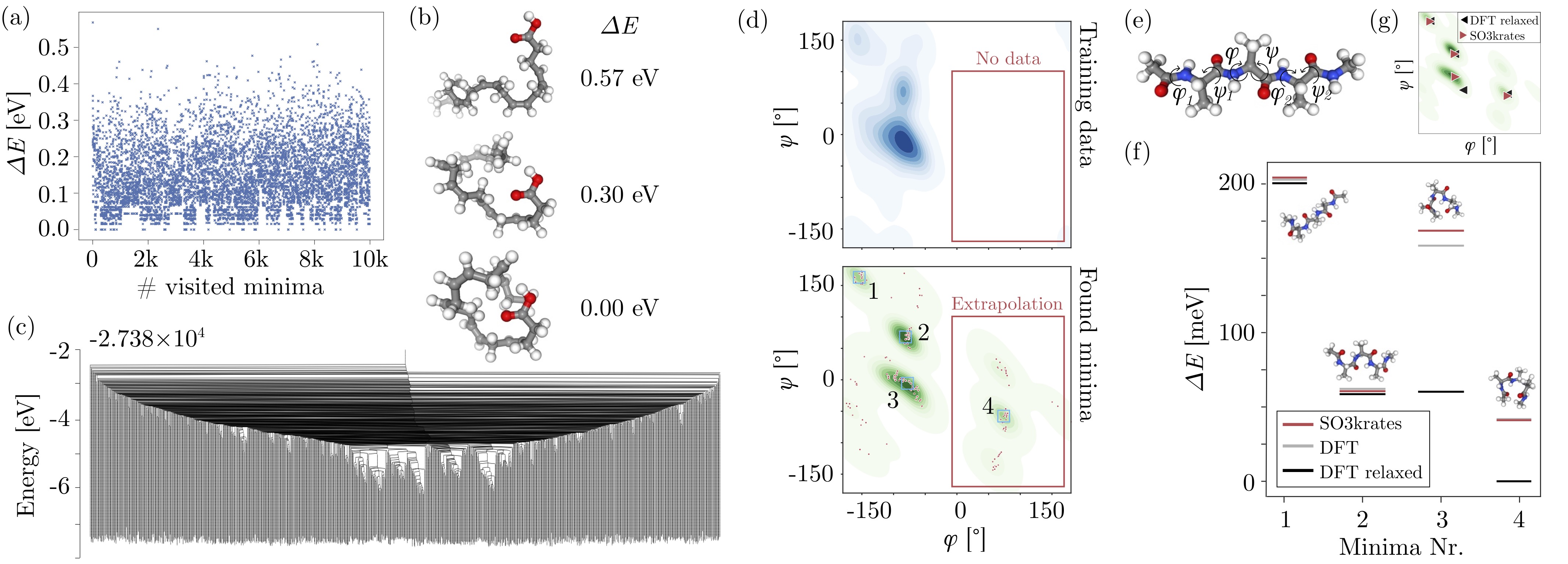
Figure 7: (a) Results of a minima search for DHA. We ran the simulation until 10k minima have been visited, which corresponds to 20M MD steps for the escape trials and to $\sim 10$M PES evaluations for the structure relaxations, afterwards. (b) Minima with the largest energy (top), the lowest energy (bottom) and an example minimum with an intermediate energy value (middle) are depicted. (c) Disconnectivity graph for all unique minima in the first 2k visited minima. Disconnectivity graphs show groups of minima at different energy levels. (d) Ramachandran density plots for the training conformations (upper, blue) and of the visited minima during minima hopping (lower, green) for two of the six backbone angles in Ac-Ala3-NHMe. Red dots correspond to the actually visited minima. Parts of the visited minima have not been in the training data, hinting towards the capability of the model to find minima beyond the training data. (e) Ac-Ala3-NHMe structure with backbone angles as inset. (f) Relative energies for four minima, which have been selected from the regions in $\psi-\phi$ space visited most frequently during minima hopping (1 - 4 in (d)). SO3krates energies are compared to a DFT single point calculation and to the conformation obtained from a full DFT relaxation starting from the minima obtained from SO3krates. (g) Location in the Ramachandran plot of the minima obtained with SO3krates and the relaxed DFT minima.

For both systems under investigation, one finds notable peaks for C-C vibrations ($500\,\text{cm}^{-1}$ and $1500\,\text{cm}^{-1}$), C-H bending ($\sim 900\,\text{cm}^{-1}$) and for high frequency C-H stretching ($\sim 3000\,\text{cm}^{-1}$). Both systems exhibit covalent and non-covalent interactions [56, 58], where e.g. van-der-Waals interactions hold the inner tube within the outer one. Although small in magnitude, we find the MLFF to yield a correct description for both interaction classes, such that the largest degree of freedom for the double walled nanotube corresponds to the rotation of the tubes w. r. t. each other, in line with the findings from [55].

For DHA, we further analyze the evolution of the velocity auto-correlation function with temperature and find non-trivial shifts in the spectrum hinting towards the capability of the model to learn non-harmonic contributions of the PES. As pointed out in [59], FFs that only rely on (learn) harmonic bond and angle approximations fail to predict changing population or temperature shifts in the middle to high frequency regime. Similar results are obtained for Ac-Ala3-NHMe (SI Fig. 11).

II.5 Potential Energy Surface Topology

The accurate description of conformational changes remains one of the hardest challenges in molecular biophysics. Every conformation is associated with a local minimum on the PES, and the count of these minima increases exponentially with system size. This limits the applicability of ab-initio methods or computationally expensive MLFFs, since even the sampling of sub-regions of the PES involves the calculation of thousands to millions of equilibrium structures. Here, we explore 10k minima for two small bio-molecules, which requires $\sim 30$M FF evaluations per simulation. This analysis would require more than a year with DFT and more than a month with previous equivariant architectures, whereas we are able to perform it in $\sim 2$ days.

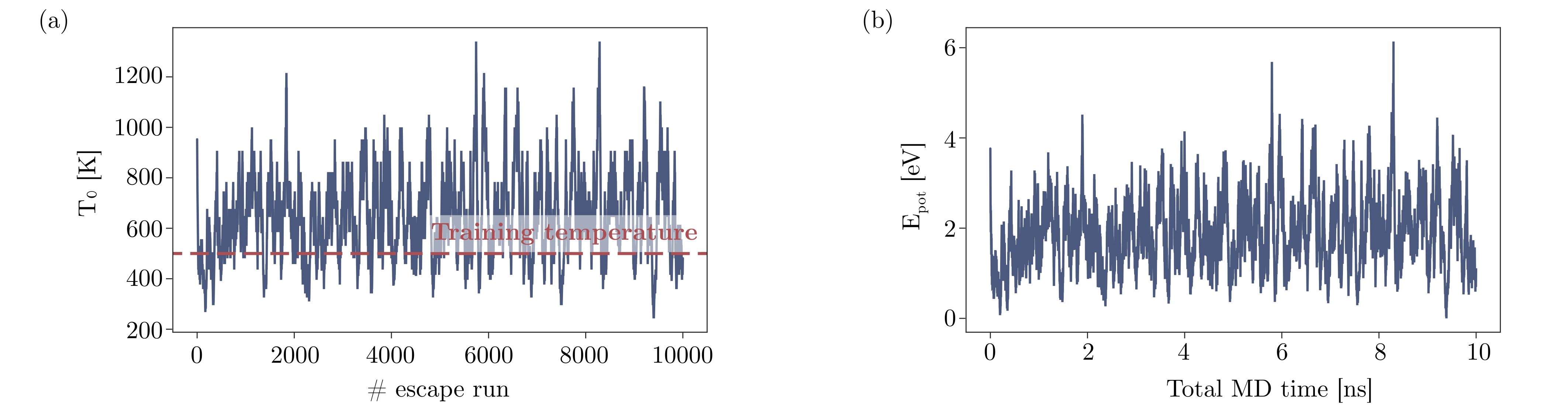
Figure 16: (a) The initial temperature $T_{0}$ for the MD simulations as a function of the MD escape run in the minima hopping algorithm. Since velocity-verlet is used for the MD simulation and the structure is in a local minima at the beginning of the MD, equipartition principle will result in an MD that has temperature $T_{0}/2$. (b) The maximal potential energy that is observed during each MD escape run vs the total MD simulation time.

We employ the minima hopping algorithm [41], which explores the PES based on short MD simulations (escapes) that are followed by structure relaxations. The MD temperature is determined dynamically, based on the history of minima already found. In that way low energy regions are explored and high energy (temperature) barriers can be crossed as soon as no new minima are found. This necessitates a fast MLFF, since each escape and structure relaxation process consists of up to a few thousands of steps. At the same time, the adaptive nature of the MD temperature, can result in temperatures larger than the training temperature (SI Fig. 16 (a)) which requires stability towards out-of-distribution geometries.

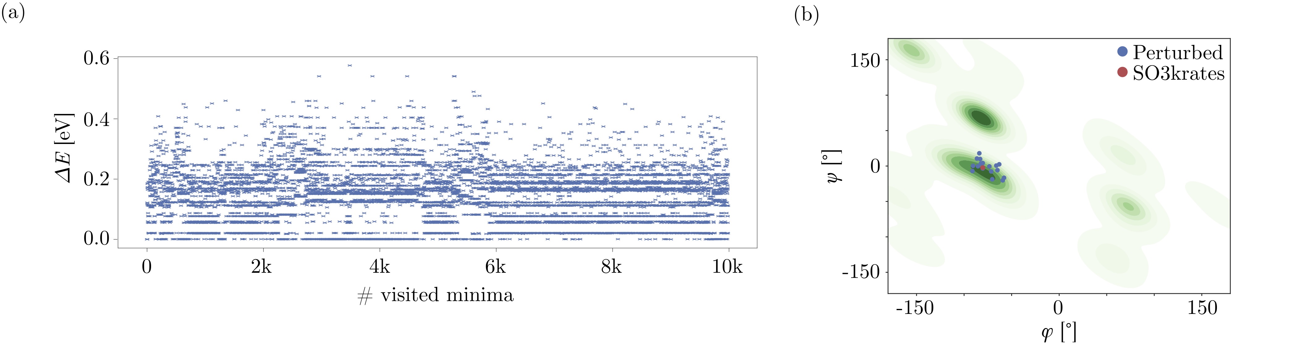
Figure 18: (a) Potential energies for the visited minima of the Ac-Ala3-NHMe structure are shown. (b) Location in the Ramachandran plot of 18 randomly perturbed structures (blue) around the original minimum (red). The location of the re-performed relaxations is also shown in red. Since all optimizations relaxed into the same, original minimum one can only see a single red dot.

We start by exploring the PES of DHA and analyse the minima that are visited during the optimization (Fig. 7 (a)). We find many minima close in energy which are associated with different foldings of the carbon chain due to van-der-Waals interactions. This is in contrast to the minimum energies found for other chainlike molecules such as Ac-Ala3-NHMe, where less local minima are found per energy unit (SI Fig. 18 (a)). The largest observed energy difference corresponds to 0.57 eV, where the minima with the largest potential energy (top) and the lowest potential energy (bottom) as well as an example structure from the intermediate energy regime (middle) are shown in Fig. 7 (b). We find the observed geometries to be in line with the expectation that higher energy configurations promote an unfolding of the carbon chain.

Funnels are sets of local minima separated to other sets of local minima by large energy barriers. The detection of folding funnels plays an important role in protein folding and finding native states, which determine biological functioning and properties of proteins. The combinatorial explosion of the number of minima configurations makes funnel detection unfeasible with ab-initio methods or computationally expensive MLFFs. We use the visited minima and the transition state energies that are estimated from the MD between successive minima to create a so-called disconnectivity graph [60]. It allows detect multiple funnels in the PES of DHA, which are separated by energy barriers up to 3 eV.

Ac-Ala-NHMe is a popular example system for bio-molecular simulations, as its conformational changes are primarily determined by Ramachandran dihedral angles. These dihedral angles also play a crucial role in representing important degrees of freedom in significantly larger peptides or proteins [61]. Here, we go beyond this simple example and use the minima hopping algorithm to explore 10k minima of Ac-Ala3-NHMe and visualize their locations in a Ramachandran plot (green in Fig. 7 (d)) for two selected backbone angles $\phi$ and $\psi$ (Fig. 7 (e)). By investigating high density minima regions and comparing them to the training data (blue in (Fig. 7 (d))), we can show that SO3krates finds minima in PES regions, which highlights the capability of the model to extrapolate beyond known conformations. Extrapolation to unknown parts of the PES is inevitable for the application of MLFFs in bio-molecular simulations, since the computational cost of DFT only allows to sample sub-regions of the PES for increasingly large structures.

To confirm the physical validity of the found minima, we select one equilibrium geometry from each of the four highest density regions in the Ramachandran plots (1 - 4 in Fig. 7 (d)). A comparison of the corresponding energies predicted by SO3krates with DFT single point calculations (Fig. 7 (f)) shows excellent agreement with a mean deviation of 3.45 meV for this set of four points. Remarkably, the minimum in the unsampled region of the PES (red box in Fig. 7 (d)) only deviates by mere 0.7 meV in energy. We further compare the SO3krates relaxed structure to structures obtained from a DFT relaxation, initiated from the same starting points. For minima 1 and 2, we again find excellent agreement with an energy error of 2.38 meV and 3.57 meV, respectively. The extrapolated minima 4 shows a slightly increased deviation (41.84 meV), which aligns with our expectation that the model performs optimally within the training data regime. Further, minima 1, 2 and 4 show good agreement with the backbone angles obtained from DFT relaxations (Fig. 7 (g)).

For minimum 3, we find the largest energy deviation w. r. t. both, DFT single point calculation and DFT relaxation. When comparing the relaxed structures, we observe that one methyl group is rotated by 180^∘, the addition of a hydrogen bond and a stronger steric strain in the SO3krates prediction. These deviations coincide with a relatively large distance in the $\phi$-$\psi$ plane (Fig. 7 (g)). To investigate the extend of minimum 3, we have generated random perturbations of the equilibrium geometry from which additional relaxation runs have been initiated. All optimizations returned into the original minimum (SI Fig. 18 (b)), confirming that it is not an artifact due to a non-smooth or noisy PES representation.

III Discussion

Long time-scale MD simulations are essential to reveal converged dynamic and thermodynamic observables of molecular systems [62, 63, 64, 65]. Despite achieving low test errors, many state-of-the-art MLFFs exhibit unpredictable behavior caused by the accumulation of unphysical contributions to the output, making it extremely difficult or even impossible to reach extended timescales [30]. This prevents the extraction of physically faithful observables at scale. Ongoing research aims at improving stability by incorporating physically meaningful inductive biases via various kinds of symmetry constraints [8, 11, 17, 66, 33, 34, 67], but the large computational cost of current solutions mitigates many practical advantages.

We overcome the challenging trade-off between stability and computational cost by combining two novel concepts - a Euclidean self-attention mechanism and the EV as efficient representation for molecular geometry - within the equivariant transformer architecture SO3krates. The exceptional performance of our approach is due to the decoupling of invariant and equivariant information, which enables a substantial reduction in computational complexity compared to other equivariant models.

Our architecture strategically emphasises the importance of the more significant invariant features over equivariant ones, resulting in a more efficient allocation of computational resources. While equivariant features carry important directional information, the core of ML inference lies in the invariant features. Only invariant features can be subjected to powerful non-linear transformations within the architecture, while equivariant features essentially have to be passed-through to the output in order to be preserved. In our implementation, the computationally cheap invariant parts ($l=0$) of the model are allowed to use significantly more parameters than the costly equivariant ones ($l>0$). Despite this heavy parameter reduction of the equivariant components, desirable properties associated with equivariant models, such as high data efficiency, reliable MD stability, and temperature extrapolation could still be preserved.

In the context of MD simulations, we found that the equivariant network (SO3krates with $l_{\rm max}>0$) gives smaller force error distributions than its invariant counterpart (SO3krates with $l_{\rm max}=0$). This effect, however, is only visible when the force error is investigated on a per-structure and not on the per-atom level. This observation indicates that the invariant network over-fits to certain structures. We also found the equivariant model to remain stable across a large range of temperatures, whereas the stability of the invariant model quickly decreases with increasing temperature. Since higher temperatures increase the probability of out-of-distribution geometries, this may hint towards a better extrapolation behavior of the equivariant model.

Applying the SO3krates architecture to different structures from the MD22 benchmark, including peptides (Ac-Ala3-NHMe, DHA) and supra-molecular structures (AT-AT, buckyball catcher, double walled nanotube), yields stable molecular dynamics (MD) simulations with impressive time scales of tens of nanoseconds per day. This enables the computation of converged velocity auto-correlation functions, allowing comparison to experimental measurements. We have also shown, that SO3krates reliably reveals conformational changes in small bio-molecules on the example of DHA and Ac-Ala3-NHMe. To that end, SO3krates is able to predict physically valid minima conformations which have not been part of the training data. The representative nature of Ac-Ala3-NHMe holds the potential that a similar behavior can be obtained for much larger peptides and proteins. The limited availability of ab-initio data for structures at this scale, makes extrapolation to unknown parts of the PES a crucial ingredient on the way to large scale bio-molecular modeling.

While our development makes stable extended simulation timescales accessible using modern MLFF modeling paradigms in an unprecedented manner, future work remains to be done in order to bring the applicability of MLFFs even closer to that of conventional classical FFs. Various encouraging avenues in that direction are currently emerging: In the current design, the EV are only defined in terms of two-body interactions. Recent results suggest that accuracy can be further improved by incorporating atomic cluster expansions into the MP step [68, 69, 47]. At the same time, this may help reducing the number of MP steps which in turn decreases the computational complexity of the model. Another, yet open discussion is the appropriate treatment of global effects. Promising steps have been taken by using low-rank approximations [24, 70], trainable Ewald summation [71] or by adding long-range corrections from continuum solvent theory [72]. Further, a recent work showed that adding long-range interactions can improve the accuracy on the MD22 benchmark [73].

Future work will therefore focus on the seamless incorporation of many-body expansions, global effects, and long-range interactions into the EV formalism and aim to further increase computational efficiency to ultimately bridge MD time-scales at high accuracy.

IV Methods

IV.1 Features and Euclidean Variables (EV)

Per-atom feature representations are initialized based on the atomic number $z_{i}$ using an embedding function

$$f_{i}=f_{\text{emb}}(z_{i}),$$ (10)

which maps the atomic number into the $F$ dimensional feature space $f_{\text{emb}}:\mathbb{N}_{+}\mapsto\mathbb{R}^{F}$.

For a given degree $l$ and order $m$, the EV are defined as

$$x_{ilm}=\frac{1}{\braket{\mathcal{N}}}\sum_{j\in\mathcal{N}(i)}\phi_{r_{\mathrm{cut}}}(r_{ij})\cdot Y^{l}_{m}(\hat{r}_{ij}),$$ (11)

where the output of $Y^{l}_{m}(\hat{r}_{ij})$ is modulated with a distance dependent cutoff function which ensures a smooth PES when atoms leave or enter the cutoff sphere. Alternatively, the EV can be initialized with all zeros, such that they are "initialized" in the first attention update 16. The aggregation is re-scaled by the average number of neighbors over the whole training data set $\braket{\mathcal{N}}$, which helps stabilizing network training. By collecting all degrees and orders up to $l_{\mathrm{max}}$ within one vector

$$\bm{x}_{i}=\big{[}x_{i00},x_{i1-1},\dots,x_{il_{\mathrm{max}}l_{\mathrm{max}}}\big{]},$$ (12)

one obtains an equivariant per-atom representation of dimension $(l_{\mathrm{max}}+1)^{2}$ which transforms according to the corresponding Wigner-D matrices.

IV.2 SO(3) Convolution Invariants

The convolution output for degree $L$ and order $M$ on the difference vector $\bm{x}_{ij}=\bm{x}_{j}-\bm{x}_{i}$ can be written as

$$x_{ij}^{LM}=\sum_{l_{1}l_{2}m_{1}m_{2}}C_{l_{1}l_{2}L}^{m_{1}m_{2}M}x_{ij}^{l1m1}x_{ij}^{l2m2}$$ (13)

where $C_{l_{1}l_{2}L}^{m_{1}m_{2}M}$ are the Clebsch-Gordan coefficients. Considering the projection on the zeroth degree $L=M=0$

$$x_{ij}^{00}=\sum_{l_{1}}\underbrace{\sum_{m_{1}}C_{l_{1}l_{1}0}^{m_{1}-m_{1}0}x_{ij}^{l1m1}x_{ij}^{l1-m1}}_{\equiv\bigoplus_{l=0}^{l_{\mathrm{max}}}\bm{x}_{ij,l\shortrightarrow 0}},$$ (14)

one can make use of the fact that $C_{l_{1}l_{2}L}^{m_{1}m_{2}M}$ is valid for $|l_{1}-l_{2}|\leq L\leq l_{1}+l_{2}$ and $M=m_{1}+m_{2}$, which corresponds to having nonzero values along the diagonal only (Fig. 2). Thus, evaluating $\bigoplus_{l=0}^{l_{\mathrm{max}}}\bm{x}_{ij,l\shortrightarrow 0}$ requires to take per-degree traces of length $(2l+1)$ and can be computed efficiently in $\mathcal{O}(l_{\mathrm{max}}^{2})$.

IV.3 Euclidean Transformer Block (ecTblock) and Euclidean Self-Attention

Given input features, EV and pairwise distance vectors the Euclidean attention block returns attended features and EV as

$$f_{i}^{\textsc{att}} =f_{i}+\sum_{j\in\mathcal{N}(i)}\phi_{r_{\mathrm{cut}}}(r_{ij})\cdot\alpha_{ij}\cdot f_{j}\,,$$ (15)

and

$$x_{ilm}^{\textsc{att}} =x_{ilm}+\sum_{j\in\mathcal{N}(i)}\phi_{r_{\mathrm{cut}}}(r_{ij})\cdot\alpha_{ijl}\cdot Y_{l}^{m}(\hat{r}_{ij})\,,$$ (16)

with a cosine cutoff function

$$\phi_{r_{\mathrm{cut}}}(r_{ij})=\frac{1}{2}\left(\cos\left(\frac{\pi r_{ij}}{r_{\mathrm{cut}}}\right)+1\right),$$ (17)

which guarantees that pairwise interactions (attention coefficients) smoothly decay to zero when atoms enter or leave the cutoff radius $r_{\mathrm{cut}}$. Eqs. (15) and Eq. (16) from above involve attention coefficients which are constructed from an equivariant attention operation (next paragraphs).

Attention coefficients are calculated as

$$\alpha_{ij}=\alpha\Big{(}f_{i},f_{j},g_{1,\dots K}(r_{ij}),\oplus_{l=0}^{l_{\mathrm{max}}}\bm{x}_{ij,l\shortrightarrow 0}\Big{)},$$ (18)

where $\bm{x}_{ij}\equiv\bm{x}_{j}-\bm{x}_{i}\in\mathbb{R}^{(l_{\mathrm{max}}+1)^{2}}$ is a relative, higher order geometric shift between neighborhoods. The function $\bigoplus_{l=0}^{l_{\mathrm{max}}}\bm{x}_{ij,l\shortrightarrow 0}$ contracts each degree in $\bm{x}_{ij}$ to the zeroth degree which results in $l_{\mathrm{max}}+1$ invariant scalars (Eq. (14)). The function $g$ expands interatomic distances in $K$ radial basis functions (RBFs)

$$g_{k}(r_{ij})=\exp{\big{(}-\gamma(\exp{(-r_{ij}})-\mu_{k})^{2}\big{)}},$$ (19)

where $\mu_{k}$ is the center of the $k$-th basis function and $\gamma$ is a function of $K$ and $r_{\mathrm{cut}}$ [17].

Based on the output of the contraction function and the RBFs we construct an $F$-dimensional filter vector as

$$w=\textsc{mlp}_{[F/4,F]}(u)+\textsc{mlp}_{[F,F]}(g),$$ (20)

where $\textsc{mlp}_{[F_{1},\dots,F_{L}]}$ denotes a multi layer perceptron network with $L$ layers, layer dimension $F_{i}$ and silu non-linearity. The first MLP acting on $u$ has a reduced dimension in the first hidden layer (since the dimension of $u$ itself is only $l_{\mathrm{max}}+1$).

Attention coefficients are then calculated using dot-product attention as

$$\alpha_{ij}=\frac{1}{\sqrt{F}}\,q_{i}^{T}(w_{ij}\odot k_{j}),$$ (21)

where $\odot$ denotes the entry-wise product and $q_{i}=Qf_{j}$ and $k_{j}=Kf_{j}$ with $K\in\mathbb{R}^{F\times F}$ and $Q\in\mathbb{R}^{F\times F}$ are trainable key and query matrices. The attention update of the features (Eq. (15)) is performed for $h$ heads in parallel. The features $f_{i}$ of dimension $F$ are split into $h$ feature heads $f_{i}^{h}$ of dimension $(h,F/h)$. From each feature head, one attention coefficient $\alpha_{ij}^{h}$ is calculated following Eq. (18) where $q_{i},k_{j}$ and $w_{ij}$ are all of dimension $F/h$. For each head, the attended features are then calculated from Eq. (15) with $f_{i}$ replaced by the corresponding head $f_{i}^{h}$. Afterwards, the heads are stacked to form again a feature vector of dimension $f_{i}$. Multi-head attention allows the model to focus on different sub-spaces in the feature representation, e.g. information about distances, angles or atomic types [39].

IV.4 Interaction Block

An interaction block (Iblock) aims to interchange per-atom information between the invariant and the geometric variables. Refinements for invariant features and equivariant EV are calculated as

$$\mathrm{d}f_{i},\mathrm{d}\bm{x}_{i}=\textsc{Iblock}\big{(}f_{i}^{\textsc{att}},\oplus_{l=0}^{l_{\mathrm{max}}}\bm{x}^{\text{att}}_{i,l\shortrightarrow 0})\big{)},$$ (22)

More specifically, the refinements are calculated as

$$\mathrm{d}f_{i}=a$$ (23)

and

$$\mathrm{d}x_{ilm}=b_{l}x_{ilm}^{\textsc{att}},$$ (24)

where $a\in\mathbb{R}^{F}$ and one $b_{l}\in\mathbb{R}$ for each degree $l$. They are calculated from a singled layered MLP as

$$a,b=\textsc{mlp}_{[f+l_{\mathrm{max}}+1]}(f_{i}^{\textsc{att}},\oplus_{l=0}^{l_{\mathrm{max}}}\bm{x}^{\text{att}}_{i,l\shortrightarrow 0})$$ (25)

such that $a$ and $b=[b_{0},\dots,b_{l_{\mathrm{max}}}]$ contain mixed information about both $f_{i}$ and $\bm{x}_{i}$. Updates are then calculated as

$$f_{i}^{[t+1]} =f_{i}^{\textsc{att}}+\mathrm{d}f_{i},$$ (26)

$$\bm{x}_{i}^{[t+1]} =\bm{x}_{i}^{\textsc{att}}+\mathrm{d}\bm{x}_{i},$$ (27)

which builds the relation to the initially stated update equations of the ecTblock and concludes the architecture description.

IV.5 MD Stability

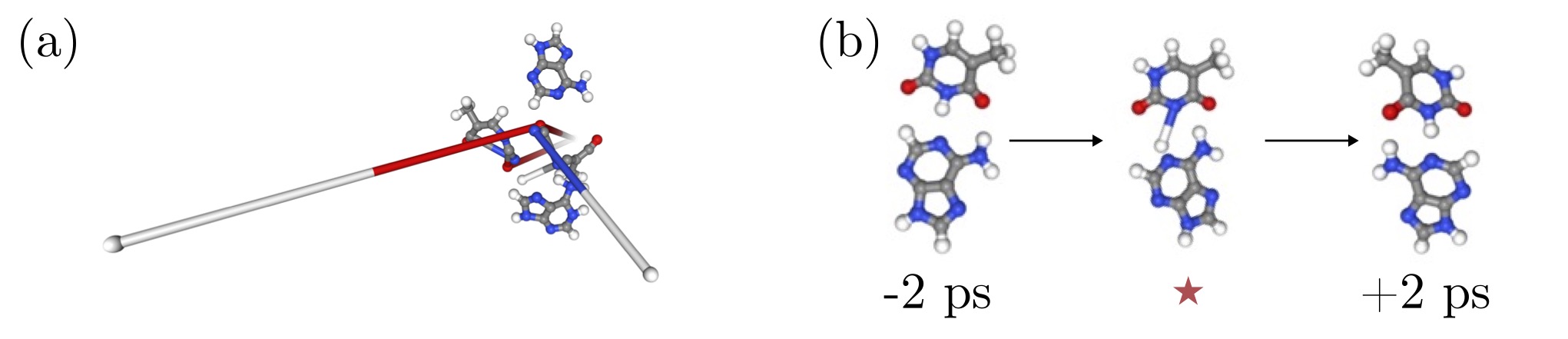
Figure 8: Potential instabilities that can occur in an MD simulation using MLFF. (a) Illustration of an "explosion" during an MD simulation. (b) Illustration of a temporarily limited instability (here the breaking of a covalent bond).

We define an MD to be stable when (A) there is an uncontrolled dissociation of the system, and (B) each bond length follows a reasonable distribution over time. We refer to failure mode (A) as an explosion of the MD simulation when (at least one of) the force predictions of the MLFF diverges during the MD simulation (Fig. 8 (a). A decomposition of (parts of) the molecule can be detected by a strong peak in MD temperature, which is usually a few orders of magnitude larger than the target temperature. We assume a bond length to be distributed reasonably, when it does not differ by more than 50 % from the equilibrium bond distance at any point of the simulation. Criteria (A) has e.g. been used in [30] to determine the MD stability of different MLFFs. However, in certain cases analysing MD temperature can be an insufficient condition to detect unstable behavior, e.g. when single bonds dissociate slowly over time or take on non-physical values over a temporarily limited interval (Fig. 8 (b)). Such a behavior, however, is easily identified using criteria (B).

A stability coefficient $c_{s}\in[0,1]$ is then calculated as

$$c_{s}=\frac{n_{s}}{n_{\text{tot}}},$$ (28)

where $n_{s}$ is the number of MD steps until an instability occurs and $n_{\text{tot}}$ is the maximal number of MD steps. When no instability is observed in the simulations we set $n_{s}=n_{\text{tot}}$.

IV.6 MD Simulations

For the MD simulation of Li₃PO₄ we chose the first conformation of in the quenched state as initial starting point. We then run the simulation for 50 ps with a time step of 2 fs using a Nose-Hoover thermostat at 600 K. For MD simulations with molecules from the MD22 data set we first chose a structure which has not been part of the training data. It is then relaxed using the LBFGS optimizer until the maximal force norm per atom is smaller than $10^{-4}\,\text{eV}$\mathrm{\SIUnitSymbolAngstrom}$^{-1}$. The relaxed structure serves as starting point for the MD simulation. For the comparison of invariant and equivariant model, we run three MD simulations per molecule from three different initial conformations with a time step of 0.5 fs and a total time of 300 ps using the Velocity Verlet algorithm without thermostat. For the calculation of the velocity-auto-correlation functions, we ran MD simulations with a time step of 0.2 fs following [55] and a total time of 1 ns. Temperatures vary between molecules and are reported in the main body of the text. Again only the Velocity Verlet without thermostat is used. We show in SI A.1, that the performed simulations are energy conserving and reach temperature equilibrium. When using the Velocity Verlet algorithm, initial velocities are drawn from a Maxwell Boltzmann distribution with a temperature twice as large as the MD target temperature. For the MD stability experiments on the MD17 molecules, we follow [30] and run simulations with a Nose-Hoover thermostat at 500 K and a time step of 0.5 fs for 300 ps.

IV.7 Minima Hopping Algorithm

For the minima hopping experiments we use the models that have been trained on the MD22 data set with 1k training samples. Each escape run corresponds to a 1 ps MD simulation with a time step of 0.5 fs using the Velocity Verlet algorithm. The following structure relaxation is performed using the LBFGS optimizer until the maximal norm per atomic force vector is smaller than $10^{-4}\,\text{eV}$\mathrm{\SIUnitSymbolAngstrom}$^{-1}$, which took around 1k optimizer steps on average. The initial velocities are drawn from the Maxwell-Boltzmann distribution at temperature $T_{0}$, which are re-scaled afterwards such that the systems temperature matches $T_{0}$ exactly. Since the structure is in a (local) minima at initialization, the equipartition principle will result in an MD which has temperature $T_{0}/2$ on average. After the MD escape run the newly proposed minima is compared to the current minima as well as to all the minima that have been visited before (history). Minima are compared based on their RMSD. To remove translations, we compare the coordinates relative to the center of mass. Also, since structures might differ by a global rotation only, we minimize the RMSD over SO(3), following the algorithm described in section 7.1.9 Rotations (p. 246-250) in [74]. If $\text{RMSD}\leq 10^{-1}$ between two minima, they are considered to be identical. If the newly proposed minima is not the current minima (i.e. it is either completely new or in the history), the new minima is accepted if the energy difference is below a certain threshold $E_{\text{diff}}$.

For the initial temperature we chose $T_{0}=1000$ K and for $E_{\text{diff}}=2$ eV. Both quantities are dynamically adjusted during runtime, where we stick to the default parameters [41]. The development of $T_{0}$ along the number of performed escape runs shows initial temperatures ranging from $\sim 300$ K up to $\sim 1300$ K (SI Fig. 16 (b)). To estimate the transition states for the connectivity graph, the largest potential energy observed between two connected minima is taken for its energy (SI Fig. 16 (b)).

IV.8 Network and Training

All SO3krates models use a feature dimension of $F=132$, $h=4$ heads in the invariant MP update and $r_{\mathrm{cut}}=5\,$\mathrm{\SIUnitSymbolAngstrom}$$. The number of MP updates and the degrees in the EV vary between experiments. For the comparison of invariant and equivariant model we use degrees $l=\{0\}$ and $l=\{0,1,2,3\}$, $T=3$ and EV initialization following Eq. (11). The invariant degree is explicitly included, in order to exclude the possibility that stability issues might come from the inclusion of degree $l=0$. The number of network parameters of the invariant model is 386k and of the equivariant model is 311k, such that the better stability is not be related to a larger parameter capacity but truly to the degree of geometric information. Due to the use of as many heads as degrees in the MP update for the EV, increasing the number of degrees results in a slightly smaller parameter number for the equivariant model. Per molecule 10,500 conformations are drawn of which 500 are used for validation. For the invariant and equivariant model, two models are trained on training data sets which are drawn with different random seeds. The model for Li₄PO₃ uses $T=2$, $l=\{1,2,3\}$ and initializes the EV to all zeros. For training, 11k samples are drawn randomly from the full data set of which 1k are used for validation, following [53].

All other models use degrees $l=\{1,2,3\}$ in the EV, $T=3$ and initialize the EV according to Eq. (11). For the MD17 stability experiments, 10,000 conformations are randomly selected of which 9,500 are used for training and 500 for validation. For the MD22 benchmark a varying number of training samples plus 500 validation samples or 1000 training samples plus 500 validation samples are drawn randomly. The models trained on 1000 samples are used for the calculation of the velocity auto-correlation functions and for the minima hopping experiments.

All models are trained on a combined loss of energy and forces

$$\mathcal{L}=(1-\beta)\cdot(E-\tilde{E})^{2}+\frac{\beta}{3N}\sum_{k=1}^{n}\sum_{i\in(x,y,z)}(F_{k}^{i}-\tilde{F}_{k}^{i})^{2},$$ (29)

where $\tilde{E}$ and $\tilde{F}$ are the ground truth and $E$ and $F$ are the predictions of the model. We use the ADAM [75] optimizer with an initial learning rate (LR) of $\eta=10^{-3}$ and a trade-off parameter of $\beta=0.99$. The LR is decreased by a factor of 0.7 every 100k training steps using exponential LR decay. Training is stopped after 1M steps. The batch sizes $B_{s}$ for training depends on the number of training points $n_{\text{train}}$, where we use $B_{s}=1$ if $n_{\text{train}}\leq 1000$ and $B_{s}=10$ if $n_{\text{train}}\geq 1000$. All presented models can be trained in less than 12h on a single NVIDIA A100 GPU.

V Code and Data Availability

The code for SO3krates is available at https://github.com/thorben-frank/mlff, which contains interfaces for model training and running MD simulations on GPU. MD17 data for stability experiments and MD22 data are freely available from http://sgdml.org/#datasets. The Li₃PO₄ data can be downloaded from https://archive.materialscloud.org/record/2022.128.

VI Acknowledgements

JTF, KRM, and SC acknowledge support by the Federal Ministry of Education and Research (BMBF) for BIFOLD (01IS18037A). KRM was partly supported by the Institute of Information & Communications Technology Planning & Evaluation (IITP) grants funded by the Korea government(MSIT) (No. 2019-0-00079, Artificial Intelligence Graduate School Program, Korea University and No. 2022-0-00984, Development of Artificial Intelligence Technology for Personalized Plug-and-Play Explanation and Verification of Explanation), and was partly supported by the German Ministry for Education and Research (BMBF) under Grants 01IS14013A-E, AIMM, 01GQ1115, 01GQ0850, 01IS18025A and 01IS18037A; the German Research Foundation (DFG). The authors would like to thank Niklas Schmitz and Mihail Bogojeski for helpful discussion. Correspondence to KRM and SC.

Supplementary Information

Appendix A SI Experiments

A.1 MD Simulations

In Fig. 9 and Fig. 10 we plot the distribution of total energy values, energies as a function of time and the temperature as a function of time for the MD simulations which have been used to calculate the velocity auto-correlation functions (main body Fig. 6). As it can be readily verified, the performed simulations are energy conserving where the total energies follow a Gaussian distribution with a small, but non-zero variance that is a consequence of the finite step size in the numerical integration performed in the Velocity-Verlet update.

Figure 11 (b) shows the velocity auto-correlation function for Ac-Ala3-NHMe at three different temperatures of 100 K, 300 K and 500 K. As reported for DHA in the main body of the text, we find non-trivial shifts in frequency and population across different temperatures. On the right hand side, we show the radial and angular distribution functions for both Ac-Ala3-NHMe and DHA at a temperature of 500 K.

A.2 Radial Distribution Functions

From the MD simulations for the small organic molecules from the MD17 data set, we further calculated radial distribution functions (RDFs) and compare them to the RDFs from DFT. The results are displayed in Fig. 12.

A.3 DHA Data Efficiency

To measure the data efficiency of DHA, we trained models with different $l_{\mathrm{max}}$ for varying $N_{\text{train}}$ and do a linear fit in the log-log space. Following [33] this allows to compare the data efficiency of the models via the slope of the fit.

A.4 Invariant vs. Equivariant

In Tab. 4 we report the parameters found by fitting a log-normal curve to the error distributions. As written in the main body of the text, we used two different error metrics. The per-atom force MSE is calculated as

$$d_{i}=\sqrt{\sum_{\alpha\in(x,y,z)}(F_{i,\alpha}-F^{\text{GT}}_{i,\alpha})^{2}}$$ (30)

and the per-structure MSE is computed as

$$D_{k}=\frac{1}{n}\sum_{i=1}^{n}d_{i},$$ (31)

involving an additional mean per structure. From the equations above its clear that the mean for both $d_{i}$ and $D_{k}$ is identical, whereas the variances can be differ.

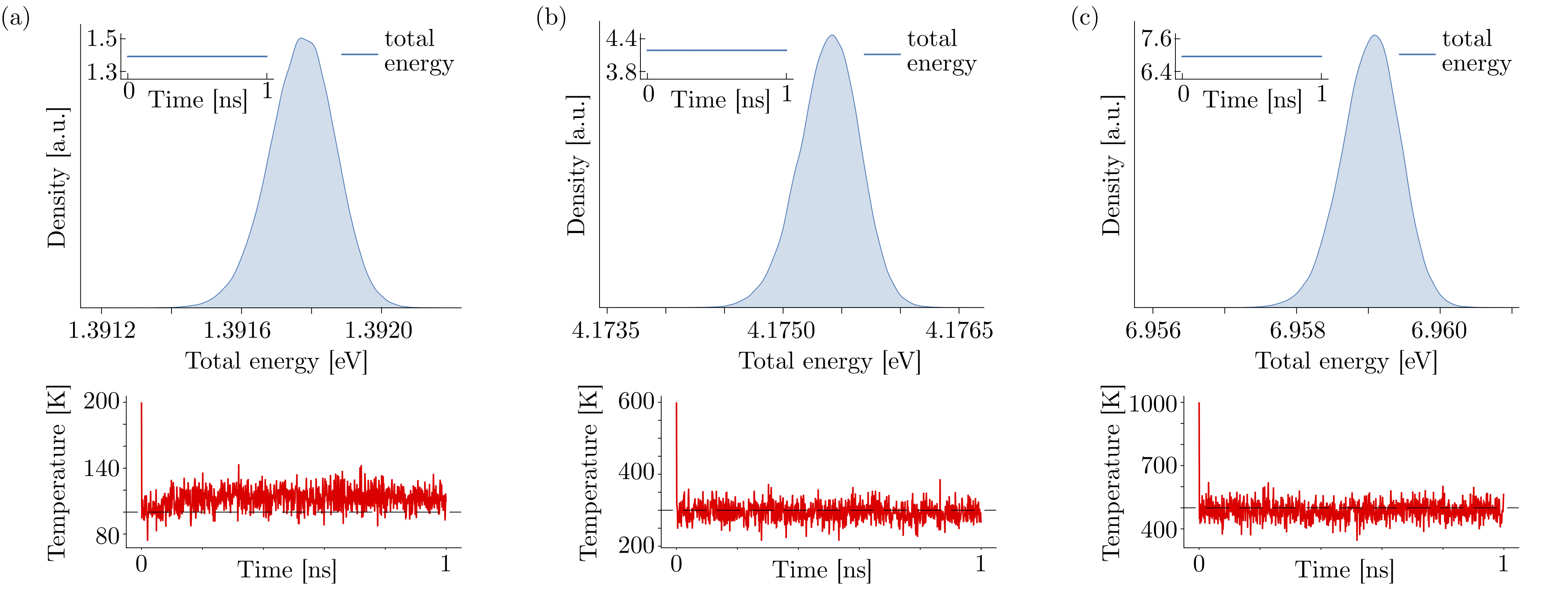
Figure 9: Total energy distribution, total energy over time (inset) and the temperature over time as observed in the MD simulations for DHA with target temperatures (a) 100 K, (b) 300 K and (c) 500 K using the Velocity-Verlet algorithm. From the resulting trajectories, the velocity auto-correlation function reported in the main body of the text have been calculated.

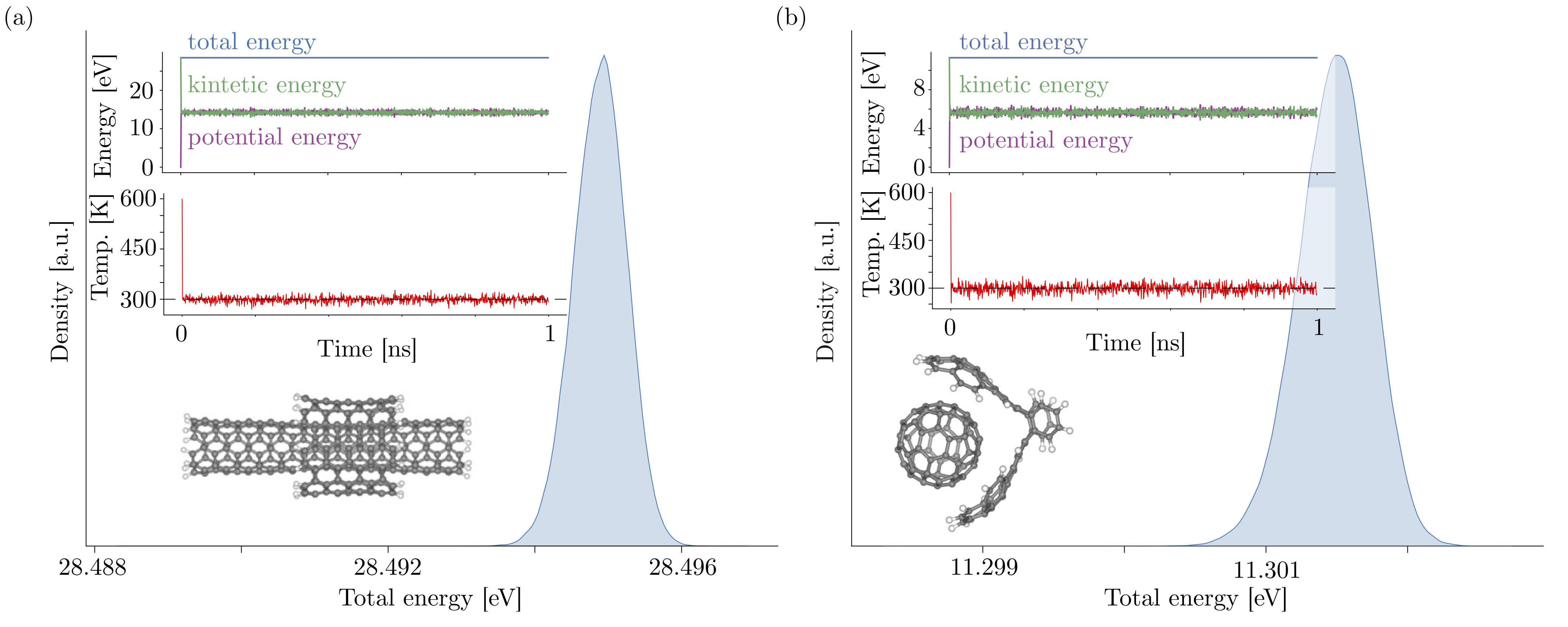
Figure 10: Total energy distribution as well as total energy, potential energy, kinetic energy and temperature as a function of time (insets) for the double walled nanotube (a) and the buckyball catcher (b). After a few ps, kinetic and potential energy reach equilibration leading to the desired target temperature of 300 K.

Figure 11: Velocity auto-correlation function for Ac-Ala3-NHMe at different temperatures obtained with the SO3krates-FF.

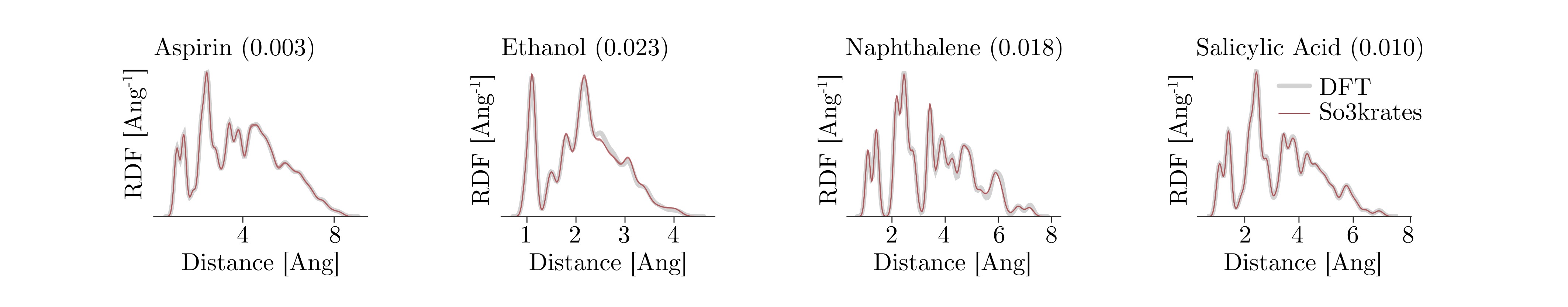
Figure 12: Radial distribution functions (RDFs) obtained from the MD simulations for which stabilities and FPS have been reported in subfigure (a). For each structure the RDF for each of the five runs is plotted, which shows that observables are stable over multiple runs and structures. The number in brackets corresponds to the MAE between the RDFs obtained from SO3krates and from DFT.

	per atom error $d_{i}$				per structure error $D_{k}$
	$l_{\mathrm{max}}=0$		$l_{\mathrm{max}}=3$		$l_{\mathrm{max}}=0$		$l_{\mathrm{max}}=3$
Ac-Ala3-NHMe	$\mu=0.051$	$s=0.641$	$\mu=0.053$	$s=0.610$	$\mu=0.051$	$s=0.269$	$\mu=0.053$	$s=0.169$
DHA	$\mu=0.083$	$s=0.591$	$\mu=0.083$	$s=0.554$	$\mu=0.083$	$s=0.198$	$\mu=0.083$	$s=0.155$
AT-AT	$\mu=0.057$	$s=0.511$	$\mu=0.055$	$s=0.243$	$\mu=0.057$	$s=0.501$	$\mu=0.055$	$s=0.186$

Table 4: Mean and spread of the per-atom MSE $d_{i}$ (cf. Eq. (30)) and of the per-structure MSE $D_{k}$ (cf. Eq. (31)) for the three different structures investigated in the main text.

A.5 Minima Hopping

A.5.1 Stable Minima

During the minima hopping algorithm the LBFGS optimization for DHA (Ac-Ala3-NHMe) did not converge in 8 (15) cases. Since they are comparably large in energy they are rejected due to $E_{\text{diff}}$ and consequently do not affect the algorithm during runtime. When comparing all minima that have been visited, however, we have to explicitly exclude them. We do this by first choosing the minima with the lowest potential energy as reference structure and calculate the bond lengths from it. Afterwards, we compare the bond lengths of all other visited minima to this reference structure and exclude them when the RMSD between all bond lengths is larger than $10^{-2}$. We note, that this allows to detect "bad" minima in a self-contained manner without the need of any re-calculations with ab-initio methods. Further, we re-calculated the minima with different optimizer settings and found the new minima to be stable. Thus, the failed optimizations were due to the hyperparameters of the optimizer and not due to the MLFF.

A.5.2 Invariant Model

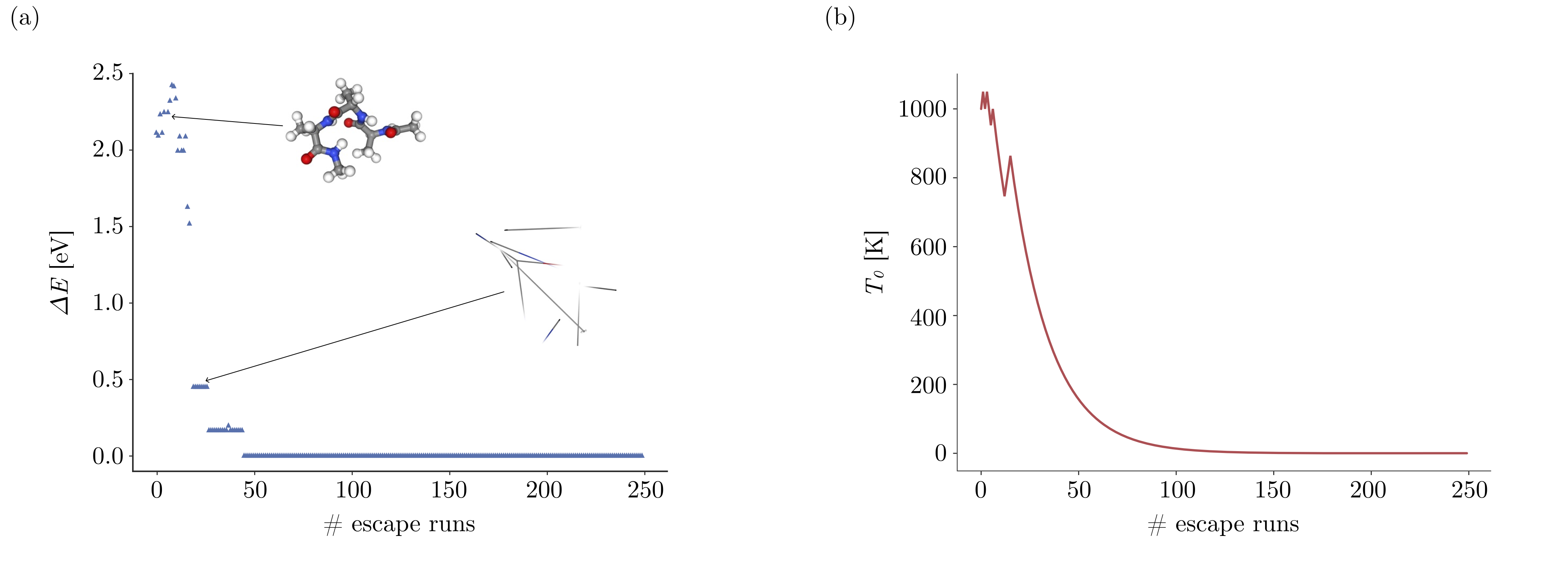
Figure 17: Figure shows the relative potential energy (a) as well as the initial temperature $T_{0}$ (b) observed during minima hopping with an invariant SO3krates model. After a few escape trials a dissociated structure is obtained as lowest energy minima. Since no lower minima is found, the initial temperature starts to decrease towards zero over escape runs.

We additionally perform the minima hopping algorithm with an invariant SO3krates model. After a few escape runs, a dissociated minima is found as lowest minima. As a consequence, no new minima can be accepted in the following and the initial temperature starts to decrease towards zero (Fig. 17). The resulting minima lead to an non-physical representation of the PES, as it can be seen in Fig. 7 in the main body of the text. For the invariant model, we chose the one from the MD stability experiments, which has been found capable of producing partially stable MDs for Ac-Ala3-NHMe (Fig. 5).

References

- Tuckerman [2002] Mark E Tuckerman. Ab initio molecular dynamics: basic concepts, current trends and novel applications. J. Phys. Condens. Matter, 14(50):R1297, 2002.
- Behler and Parrinello [2007] Jörg Behler and Michele Parrinello. Generalized neural-network representation of high-dimensional potential-energy surfaces. Phys. Rev. Lett., 98(14):146401, 2007.
- Bartók et al. [2010] Albert P Bartók, Mike C Payne, Risi Kondor, and Gábor Csányi. Gaussian Approximation Potentials: the accuracy of quantum mechanics, without the electrons. Phys. Rev. Lett., 104(13):136403, 2010.
- Behler [2011] Jörg Behler. Atom-centered symmetry functions for constructing high-dimensional neural network potentials. J. Chem. Phys., 134(7):074106, 2011.
- Rupp et al. [2012] Matthias Rupp, Alexandre Tkatchenko, Klaus-Robert Müller, and O Anatole Von Lilienfeld. Fast and accurate modeling of molecular atomization energies with machine learning. Phys. Rev. Lett., 108(5):058301, 2012.
- Bartók et al. [2013] Albert P Bartók, Risi Kondor, and Gábor Csányi. On representing chemical environments. Phys. Rev. B, 87(18):184115, 2013.
- Li et al. [2015] Zhenwei Li, James R Kermode, and Alessandro De Vita. Molecular dynamics with on-the-fly machine learning of quantum-mechanical forces. Phys. Rev. Lett., 114(9):096405, 2015.
- Chmiela et al. [2017] Stefan Chmiela, Alexandre Tkatchenko, Huziel E Sauceda, Igor Poltavsky, Kristof T Schütt, and Klaus-Robert Müller. Machine learning of accurate energy-conserving molecular force fields. Sci. Adv., 3(5):e1603015, 2017.
- Schütt et al. [2017] Kristof T Schütt, Farhad Arbabzadah, Stefan Chmiela, Klaus-Robert Müller, and Alexandre Tkatchenko. Quantum-chemical insights from deep tensor neural networks. Nat. Commun., 8:13890, 2017.
- Gastegger et al. [2017] Michael Gastegger, Jörg Behler, and Philipp Marquetand. Machine learning molecular dynamics for the simulation of infrared spectra. Chem. Sci., 8(10):6924–6935, 2017.
- Chmiela et al. [2018] Stefan Chmiela, Huziel E. Sauceda, Klaus-Robert Müller, and Alexandre Tkatchenko. Towards exact molecular dynamics simulations with machine-learned force fields. Nat. Commun., 9(1):3887, 2018. doi: 10.1038/s41467-018-06169-2.
- Schütt et al. [2018] Kristof T Schütt, Huziel E Sauceda, Pieter-Jan Kindermans, Alexandre Tkatchenko, and Klaus-Robert Müller. SchNet – a deep learning architecture for molecules and materials. J. Chem. Phys., 148(24):241722, 2018.
- Smith et al. [2017] Justin S Smith, Olexandr Isayev, and Adrian E Roitberg. ANI-1: an extensible neural network potential with DFT accuracy at force field computational cost. Chem. Sci., 8(4):3192–3203, 2017.
- Lubbers et al. [2018] Nicholas Lubbers, Justin S Smith, and Kipton Barros. Hierarchical modeling of molecular energies using a deep neural network. J. Chem. Phys., 148(24):241715, 2018.
- Stöhr et al. [2020] Martin Stöhr, Leonardo Medrano Sandonas, and Alexandre Tkatchenko. Accurate many-body repulsive potentials for density-functional tight-binding from deep tensor neural networks. J. Phys. Chem. Lett., 11:6835–6843, 2020.
- Faber et al. [2018] Felix A Faber, Anders S Christensen, Bing Huang, and O Anatole von Lilienfeld. Alchemical and structural distribution based representation for universal quantum machine learning. J. Chem. Phys., 148(24):241717, 2018.
- Unke and Meuwly [2019] Oliver T Unke and Markus Meuwly. PhysNet: A neural network for predicting energies, forces, dipole moments, and partial charges. J. Chem. Theory Comput., 15(6):3678–3693, 2019.
- Christensen et al. [2020] Anders S Christensen, Lars A Bratholm, Felix A Faber, and O Anatole von Lilienfeld. FCHL revisited: faster and more accurate quantum machine learning. J. Chem. Phys., 152(4):044107, 2020.
- Zhang et al. [2019] Yaolong Zhang, Ce Hu, and Bin Jiang. Embedded Atom Neural Network Potentials: efficient and accurate machine learning with a physically inspired representation. J. Phys. Chem. Lett., 10(17):4962–4967, 2019.
- Käser et al. [2020] Silvan Käser, Oliver Unke, and Markus Meuwly. Reactive dynamics and spectroscopy of hydrogen transfer from neural network-based reactive potential energy surfaces. New J. Phys., 22:55002, 2020.
- Noé et al. [2020] Frank Noé, Alexandre Tkatchenko, Klaus-Robert Müller, and Cecilia Clementi. Machine learning for molecular simulation. Annu. Rev. Phys. Chem., 71:361–390, 2020.
- von Lilienfeld et al. [2020] O Anatole von Lilienfeld, Klaus-Robert Müller, and Alexandre Tkatchenko. Exploring chemical compound space with quantum-based machine learning. Nat. Rev. Chem., 4(7):347–358, 2020.
- Unke et al. [2021a] Oliver T Unke, Stefan Chmiela, Huziel E Sauceda, Michael Gastegger, Igor Poltavsky, Kristof T Schütt, Alexandre Tkatchenko, and Klaus-Robert Müller. Machine learning force fields. Chem. Rev., 121(16):10142–10186, 2021a.
- Unke et al. [2021b] Oliver T Unke, Stefan Chmiela, Michael Gastegger, Kristof T Schütt, Huziel E Sauceda, and Klaus-Robert Müller. SpookyNet: Learning force fields with electronic degrees of freedom and nonlocal effects. Nat. Commun., 12:7273, 2021b.
- Unke et al. [2022] Oliver T Unke, Martin Stöhr, Stefan Ganscha, Thomas Unterthiner, Hartmut Maennel, Sergii Kashubin, Daniel Ahlin, Michael Gastegger, Leonardo Medrano Sandonas, Alexandre Tkatchenko, and Klaus-Robert Müller. Accurate machine learned quantum-mechanical force fields for biomolecular simulations. arXiv preprint arXiv:2205.08306, 2022.
- Smith et al. [2020] Justin S Smith, Roman Zubatyuk, Benjamin Nebgen, Nicholas Lubbers, Kipton Barros, Adrian E Roitberg, Olexandr Isayev, and Sergei Tretiak. The ani-1ccx and ani-1x data sets, coupled-cluster and density functional theory properties for molecules. Sci. Data, 7(1):1–10, 2020.
- Hoja et al. [2021] Johannes Hoja, Leonardo Medrano Sandonas, Brian G Ernst, Alvaro Vazquez-Mayagoitia, Robert A DiStasio Jr, and Alexandre Tkatchenko. Qm7-x, a comprehensive dataset of quantum-mechanical properties spanning the chemical space of small organic molecules. Sci. Data, 8(1):1–11, 2021.
- Miksch et al. [2021] April M Miksch, Tobias Morawietz, Johannes Kästner, Alexander Urban, and Nongnuch Artrith. Strategies for the construction of machine-learning potentials for accurate and efficient atomic-scale simulations. Mach. Learn. Sci. Technol., 2(3):031001, 2021.
- Stocker et al. [2022] Sina Stocker, Johannes Gasteiger, Florian Becker, Stephan Günnemann, and Johannes T Margraf. How robust are modern graph neural network potentials in long and hot molecular dynamics simulations? Mach. Learn. Sci. Technol., 3(4):045010, 2022.
- Fu et al. [2022] Xiang Fu, Zhenghao Wu, Wujie Wang, Tian Xie, Sinan Keten, Rafael Gomez-Bombarelli, and Tommi Jaakkola. Forces are not enough: Benchmark and critical evaluation for machine learning force fields with molecular simulations. arXiv preprint arXiv:2210.07237, 2022.
- Gilmer et al. [2017] Justin Gilmer, Samuel S Schoenholz, Patrick F Riley, Oriol Vinyals, and George E Dahl. Neural message passing for quantum chemistry. In International Conference on Machine Learning, pages 1263–1272. Pmlr, 2017.
- Chmiela et al. [2019] Stefan Chmiela, Huziel E Sauceda, Igor Poltavsky, Klaus-Robert Müller, and Alexandre Tkatchenko. sgdml: Constructing accurate and data efficient molecular force fields using machine learning. Comput. Phys. Commun., 240:38–45, 2019.
- Batzner et al. [2022] Simon Batzner, Albert Musaelian, Lixin Sun, Mario Geiger, Jonathan P Mailoa, Mordechai Kornbluth, Nicola Molinari, Tess E Smidt, and Boris Kozinsky. E (3)-equivariant graph neural networks for data-efficient and accurate interatomic potentials. Nat. Commun., 13(1):2453, 2022.
- Schütt et al. [2021] Kristof Schütt, Oliver Unke, and Michael Gastegger. Equivariant message passing for the prediction of tensorial properties and molecular spectra. In International Conference on Machine Learning, pages 9377–9388. PMLR, 2021.
- Frank et al. [2022] Thorben Frank, Oliver Unke, and Klaus-Robert Müller. So3krates: Equivariant attention for interactions on arbitrary length-scales in molecular systems. Advances in Neural Information Processing Systems, 35:29400–29413, 2022.
- Stark et al. [2023] Wojciech G Stark, Julia Westermayr, Oscar A Douglas-Gallardo, James Gardner, Scott Habershon, and Reinhard J Maurer. Importance of equivariant features in machine-learning interatomic potentials for reactive chemistry at metal surfaces. arXiv preprint arXiv:2305.10873, 2023.
- Thomas et al. [2018] Nathaniel Thomas, Tess Smidt, Steven Kearnes, Lusann Yang, Li Li, Kai Kohlhoff, and Patrick Riley. Tensor field networks: rotation-and translation-equivariant neural networks for 3D point clouds. arXiv preprint arXiv:1802.08219, 2018.
- Klicpera et al. [2021] Johannes Klicpera, Florian Becker, and Stephan Günnemann. Gemnet: Universal directional graph neural networks for molecules. arXiv preprint arXiv:2106.08903, 2021.
- Vaswani et al. [2017] Ashish Vaswani, Noam Shazeer, Niki Parmar, Jakob Uszkoreit, Llion Jones, Aidan N Gomez, Lukasz Kaiser, and Illia Polosukhin. Attention is all you need. arXiv preprint arXiv:1706.03762, 2017.
- Satorras et al. [2021] Victor Garcia Satorras, Emiel Hoogeboom, and Max Welling. E (n) equivariant graph neural networks. In International Conference on Machine Learning, pages 9323–9332. PMLR, 2021.
- Goedecker [2004] Stefan Goedecker. Minima hopping: An efficient search method for the global minimum of the potential energy surface of complex molecular systems. J. Chem. Phys., 120(21):9911–9917, 2004.
- Schölkopf et al. [1998] Bernhard Schölkopf, Alexander Smola, and Klaus-Robert Müller. Nonlinear component analysis as a kernel eigenvalue problem. Neural Comput., 10(5):1299–1319, 1998.
- Vapnik [1999] Vladimir Vapnik. The nature of statistical learning theory. Springer science & business media, 1999.
- Braun et al. [2008] Mikio L Braun, Joachim M Buhmann, and Klaus-Robert Müller. On relevant dimensions in kernel feature spaces. The Journal of Machine Learning Research, 9:1875–1908, 2008.
- Klicpera et al. [2020] Johannes Klicpera, Janek Groß, and Stephan Günnemann. Directional message passing for molecular graphs. arXiv preprint arXiv:2003.03123, 2020.
- Frank and Chmiela [2021] Thorben Frank and Stefan Chmiela. Detect the interactions that matter in matter: Geometric attention for many-body systems. arXiv preprint arXiv:2106.02549, 2021.
- Batatia et al. [2022] Ilyes Batatia, David P Kovacs, Gregor Simm, Christoph Ortner, and Gábor Csányi. Mace: Higher order equivariant message passing neural networks for fast and accurate force fields. Advances in Neural Information Processing Systems, 35:11423–11436, 2022.
- Pozdnyakov et al. [2020] Sergey N Pozdnyakov, Michael J Willatt, Albert P Bartók, Christoph Ortner, Gábor Csányi, and Michele Ceriotti. Incompleteness of atomic structure representations. Phys. Rev. Lett., 125(16):166001, 2020.
- Thölke and De Fabritiis [2021] Philipp Thölke and Gianni De Fabritiis. Equivariant transformers for neural network based molecular potentials. In International Conference on Learning Representations, 2021.
- Hu et al. [2021] Weihua Hu, Muhammed Shuaibi, Abhishek Das, Siddharth Goyal, Anuroop Sriram, Jure Leskovec, Devi Parikh, and C Lawrence Zitnick. Forcenet: A graph neural network for large-scale quantum calculations. arXiv preprint arXiv:2103.01436, 2021.
- Liu et al. [2021] Yi Liu, Limei Wang, Meng Liu, Yuchao Lin, Xuan Zhang, Bora Oztekin, and Shuiwang Ji. Spherical message passing for 3d molecular graphs. In International Conference on Learning Representations, 2021.
- Lu et al. [2019] Lu Lu, Pengzhan Jin, and George Em Karniadakis. DeepONet: Learning nonlinear operators for identifying differential equations based on the universal approximation theorem of operators. arXiv preprint arXiv:1910.03193, 2019.
- Musaelian et al. [2023] Albert Musaelian, Simon Batzner, Anders Johansson, Lixin Sun, Cameron J Owen, Mordechai Kornbluth, and Boris Kozinsky. Learning local equivariant representations for large-scale atomistic dynamics. Nat. Commun., 14(1):579, 2023.
- Thompson et al. [2022] Aidan P Thompson, H Metin Aktulga, Richard Berger, Dan S Bolintineanu, W Michael Brown, Paul S Crozier, Pieter J in’t Veld, Axel Kohlmeyer, Stan G Moore, Trung Dac Nguyen, et al. Lammps-a flexible simulation tool for particle-based materials modeling at the atomic, meso, and continuum scales. Comput. Phys. Commun., 271:108171, 2022.
- Chmiela et al. [2023] Stefan Chmiela, Valentin Vassilev-Galindo, Oliver T Unke, Adil Kabylda, Huziel E Sauceda, Alexandre Tkatchenko, and Klaus-Robert Müller. Accurate global machine learning force fields for molecules with hundreds of atoms. Sci. Adv., 9(2):eadf0873, 2023.
- DiStasio et al. [2014] Robert A DiStasio, Vivekanand V Gobre, and Alexandre Tkatchenko. Many-body van der waals interactions in molecules and condensed matter. J. Phys. Condens. Matter., 26(21):213202, 2014.
- Roduner [2006] Emil Roduner. Size matters: why nanomaterials are different. Chem. Soc. Rev., 35(7):583–592, 2006.
- Kimoto et al. [2005] Yoshihisa Kimoto, Hideki Mori, Tomohito Mikami, Seiji Akita, Yoshikazu Nakayama, Kenji Higashi, and Yoshihiko Hirai. Molecular dynamics study of double-walled carbon nanotubes for nano-mechanical manipulation. Jpn. J. Appl. Phys., 44(4R):1641, 2005.
- Sauceda et al. [2020] Huziel E Sauceda, Michael Gastegger, Stefan Chmiela, Klaus-Robert Müller, and Alexandre Tkatchenko. Molecular force fields with gradient-domain machine learning (gdml): Comparison and synergies with classical force fields. J. Chem. Phys., 153(12):124109, 2020.
- Becker and Karplus [1997] Oren M Becker and Martin Karplus. The topology of multidimensional potential energy surfaces: Theory and application to peptide structure and kinetics. J. Chem. Phys., 106(4):1495–1517, 1997.
- Spiwok et al. [2008] Vojtěch Spiwok, Blanka Králová, and Igor Tvaroška. Continuous metadynamics in essential coordinates as a tool for free energy modelling of conformational changes. J. Mol. Model., 14:995–1002, 2008.
- Lindorff-Larsen et al. [2012] Kresten Lindorff-Larsen, Nikola Trbovic, Paul Maragakis, Stefano Piana, and David E Shaw. Structure and dynamics of an unfolded protein examined by molecular dynamics simulation. Journal of the American Chemical Society, 134(8):3787–3791, 2012.
- Westermayr et al. [2019] Julia Westermayr, Michael Gastegger, Maximilian FSJ Menger, Sebastian Mai, Leticia González, and Philipp Marquetand. Machine learning enables long time scale molecular photodynamics simulations. Chemical science, 10(35):8100–8107, 2019.
- Langer et al. [2023a] Marcel F Langer, Florian Knoop, Christian Carbogno, Matthias Scheffler, and Matthias Rupp. Heat flux for semi-local machine-learning potentials. arXiv preprint arXiv:2303.14434, 2023a.
- Langer et al. [2023b] Marcel F Langer, J Thorben Frank, and Florian Knoop. Stress and heat flux via automatic differentiation. arXiv preprint arXiv:2305.01401, 2023b.
- Anderson et al. [2019] Brandon Anderson, Truong-Son Hy, and Risi Kondor. Cormorant: covariant molecular neural networks. arXiv preprint arXiv:1906.04015, 2019.
- Schmitz et al. [2022] Niklas F Schmitz, Klaus-Robert Müller, and Stefan Chmiela. Algorithmic differentiation for automated modeling of machine learned force fields. J. Phys. Chem. Lett., 13(43):10183–10189, 2022.
- Drautz [2019] Ralf Drautz. Atomic cluster expansion for accurate and transferable interatomic potentials. Phys. Rev. B, 99(1):014104, 2019.
- Drautz and Ortner [2022] Ralf Drautz and Christoph Ortner. Atomic cluster expansion and wave function representations. arXiv preprint arXiv:2206.11375, 2022.
- Blücher et al. [2023] Stefan Blücher, Klaus-Robert Müller, and Stefan Chmiela. Reconstructing kernel-based machine learning force fields with superlinear convergence. J. Chem. Theory Comput., 2023.
- Yu et al. [2022] Hongyu Yu, Liangliang Hong, Shiyou Chen, Xingao Gong, and Hongjun Xiang. Capturing long-range interaction with reciprocal space neural network. arXiv preprint arXiv:2211.16684, 2022.
- Pagotto et al. [2022] Joshua Pagotto, Junji Zhang, and Timothy Duignan. Predicting the properties of salt water using neural network potentials and continuum solvent theory. 2022.
- Li et al. [2023] Yunyang Li, Yusong Wang, Lin Huang, Han Yang, Xinran Wei, Jia Zhang, Tong Wang, Zun Wang, Bin Shao, and Tie-Yan Liu. Long-short-range message-passing: A physics-informed framework to capture non-local interaction for scalable molecular dynamics simulation. arXiv preprint arXiv:2304.13542, 2023.
- Barfoot [2017] Timothy D Barfoot. State estimation for robotics. Cambridge University Press, 2017.
- Kingma and Ba [2014] Diederik P Kingma and Jimmy Ba. Adam: a method for stochastic optimization. arXiv preprint arXiv:1412.6980, 2014.