Quadratic Detection in Noncoherent Massive SIMO Systems over Correlated Channels

Abstract

With the goal of enabling ultrareliable and low-latency wireless communications for industrial internet of things (IIoT), this paper studies the use of energy-based modulations in noncoherent massive single input multiple output (SIMO)systems. We consider a one-shot communication over a channel with correlated Rayleigh fading and colored Gaussian noise. We first provide a theoretical analysis on the limitations of non-negative pulse-amplitude modulation (PAM)in systems of this kind, based on maximum likelihood detection. The existence of a fundamental error floor at high signal-to-noise ratio (SNR)regimes is proved for constellations with more than two energy levels, when no (statistical) channel state information is available at the transmitter. In the main body of the paper, we present a design framework for quadratic detectors that generalizes the widely-used energy detector, to better exploit the statistical knowledge of the channel. This allows us to design receivers optimized according to information-theoretic criteria that exhibit lower error rates at moderate and high SNR. We subsequently derive an analytic approximation for the error probability of a general class of quadratic detectors in the large array regime. Finally, we introduce an improved reception scheme based on the combination of quadratic detectors and assess its capabilities numerically.

I Introduction

Industrial internet of things (IIoT) is envisioned as the most promising extension of the already well-established internet of things (IoT). It has been attracting significant attention from both public and private sectors, since it is the key enabler for many promising applications that will impact both business and society as a whole. Some examples of such new applications are smart-grid energy management, smart cities, interconnected medical systems and autonomous drones [1].

In short, IoT is the interconnection and management of intelligent devices with almost no human intervention, mainly focusing on low-power consumer applications. On the contrary, its evolved form IIoT is targeted to mission-critical industrial cases [2]. The wireless networks involved in these scenarios are usually characterized by a high density of low-power/low-complexity terminals, the majority of which are inactive most of the time. The information being transmitted through these networks mainly consists in control and telemetry data collected by machine sensors. Therefore, while the volume of traffic is low, its transmission must be highly reliable and fulfill stringent latency constraints. To accomplish these challenging requirements, IIoT leverages two operation modes of the fifth generation (5G) of wireless systems: massive machine-type communication (mMTC)and ultra-reliable and low-latency communication (URLLC) [3].

Achieving high reliability over wireless links is challenging due to the instability of the physical medium, caused by fading, interference and other phenomena. To combat them, high diversity is of upmost importance, which can be achieved in time, frequency or space [4]. Traditionally, time and frequency have been the two main domains from which wireless systems have obtained diversity. However, they are not suitable for the development of IIoT. On the one hand, time diversity is antagonistic to the low-latency requirements. On the other, the scarcity in spectral resources is aggravated by the deployment of massive networks of terminals using frequency diversity. Therefore, the most fitting solution is spatial diversity, obtained from the use of arrays with many antennas [5]. In particular, single input multiple output (SIMO)architectures seem like a natural choice to implement the communication from machine devices to a central node. While most terminals in an IIoT network are power- and complexity-limited, the central node can allocate a large amount of antennas (i.e. massive arrays), which result in even more dramatic diversity gains [6].

The use of large arrays in SIMO architectures (i.e. massive SIMO) entails several benefits over its conventional counterpart. For instance, small-scale fading and noise effects decrease as the number of antennas increases. This stabilization of channel statistics is known as channel hardening [7, Ch. 1.3] (comparable to sphere hardening [8, Ch. 5.1.2]). To exploit this phenomenon, it is usually required for the receiver to acquire instantaneous channel state information (CSI), and implement coherent detection of the transmitted data with it. The estimation of this CSI is usually performed within a training phase, whose complexity increases with the number of antennas. In a regime such as IIoT, the size of training packets can be comparable to the short data payloads transmitted, which is problematic in terms of latency. The fraction of resources spent in instantaneous CSI acquisition is aggravated in high-mobility scenarios [4]. To combat these limitations, a noncoherent approach can be adopted, in which neither the transmitter nor the receiver have instantaneous CSI. Instead, these schemes are able to communicate and exploit channel hardening by using statistical CSI (i.e. knowledge about the channel and noise distributions), whose acquisition requires simpler training because it changes much more slowly [9, Ch. 4.5].

Many authors have studied the problem of noncoherent SIMO systems for URLLC applications and have envisioned schemes based on energy detection [10, 11, 4, 12, 13]. Most works in the literature are based on the energy detector (ED)scheme [5]. It arises naturally as a special case of the maximum likelihood (ML)detector and uses the squared norm of the received signal as its statistic. These designs are optimal under uncorrelated Rayleigh fading, in which the used statistic is sufficient, and allow for low-complexity implementations. Furthermore, energy-based noncoherent schemes display the same rate scaling behaviour (in terms of receiver antennas) as their coherent counterparts [5].

Despite the analytical simplicity entailed by isotropic channels, it is an unrealistic model for fading statistics when using massive arrays [14]. The noncoherent energy-based setting for arbitrary fading remains mostly unexplored in the literature. A notable exception is [13], in which the ML detector is analysed under correlated fading and an optimized constellation design is developed. The main drawback against using the ML detector is the fact that its complexity is much higher than that of ED. Nevertheless, using ED under non-isotropic fading is sub-optimal and its performance is severely degraded by channel correlation, as explored in [15]. The statistic used by ED is not sufficient under general fading and, therefore, does not fully exploit the knowledge of second order moments of the channel.

In this paper, we consider a noncoherent, energy-based massive SIMO system in which a single-antenna terminal communicates to a central node equipped with a large array over a correlated Rayleigh fading channel. Statistical CSI is available at the receiver but not at the transmitter, which is low-complexity, as is common in many IIoT implementations [16]. Information is modulated on the transmitted energy and the receiver decodes it symbol-by-symbol (i.e. one-shot scheme), thus a one-sided pulse-amplitude modulation (PAM)constellation is adopted. Contrary to existing approaches, we propose a simplified detector architecture that thoroughly exploits statistical CSI (hence generalizing ED) but whose complexity does not scale with constellation size, as is the case with ML detection.

We now provide a brief summary of the main contributions of this work, displayed in the same order they are found in the text:

• In Section II, the problem of interest is formulated and analysed asymptotically for signal-to-noise ratio (SNR)and number of antennas. We formally prove the use of a uniquely factorable constellation (UFC) [17] is a sufficient condition for the error probability to vanish as the number of antennas increases (Theorem 1). On the contrary, we show unique factorization is insufficient to arbitrarily reduce error probability by increasing SNR in constellations with more than two symbols (Theorem 2). To do so, we prove the existence of a fundamental error floor at high SNR, whose characterization is of upmost importance in the context of energy efficiency for IIoT. This result generalizes related ones from [11], in which the authors establish a high SNR error floor under isotropic Rayleigh fading and attribute it to channel energy uncertainties. Similar phenomena are also observed numerically in [15, 12]. Note that this issue is not present when the transmitter can exploit statistical CSI by employing optimized constellations that adapt to each SNR level [4].

• In Section III, we introduce a general symbol detection framework based on quadratic energy statistics, for which ED is a simple case. Its structure allows to decouple the reception into an estimation phase and a decision one. To deal with the first step, we derive the Bayesian quadratic minimum mean squared error (QMMSE)estimator, which arises naturally from an optimization problem based on information-theoretic criteria. As a byproduct, we obtain the best quadratic unbiased estimator (BQUE)for the signal energy at the receiver, and prove it is an unbiased estimator whose variance reaches the Cramér-Rao bound (CRB). We additionally show it is unrealizable, revealing the minimum variance unbiased estimator (MVUE)does not exist for such scenario.

• Section IV deals with the decision step. By use of the central limit theorem (CLT), we are able to approximate the output distribution of the previous estimator for a large number of antennas. This allows us to obtain an algorithm (Algorithm 1) to find suitable detection thresholds, as well as a simple analytic expression for the error probability, as a sum of $\mathrm{Q}$-functions. This section ends with the introduction of an improved detection scheme, the assisted best quadratic unbiased estimator (ABQUE), which consists in plugging the output of the ED into the design of the BQUE.

• Finally, in Section V, we assess the performance of the presented detectors in terms of average symbol error rate (SER)using Montecarlo simulations. In particular, ABQUE displays close to ML performance in most regimes, while the other quadratic detectors greatly outperform ED under correlated channels. Furthermore, the previously derived analytic approximations for error probabilities match these numerical results.

The following notation is used throughout the text. Boldface lowercase and uppercase letters denote vectors and matrices, respectively. Given a matrix $\mathbf{A}$, the element in its row $r$ and column $c$ is denoted as $[\mathbf{A}]_{r,c}$. The transpose operator is $\cdot^{\mathrm{T}}$ and the conjugate transpose one is $\cdot^{\mathrm{H}}$. The trace operator is $\mathrm{tr}(\cdot)$, the determinant of a matrix $\mathbf{A}$ is given by $|\mathbf{A}|$ and its Frobenius norm is $\|\mathbf{A}\|_{\mathrm{F}}\triangleq\sqrt{\mathrm{tr}(\mathbf{A}^{\mathrm{H}}\mathbf{A})}$. The sets of real and complex numbers are $\mathbb{R}$ and $\mathbb{C}$, respectively. The imaginary unit is represented with $\mathrm{j}$, and the real and imaginary parts of a complex number are $\mathrm{Re}(\cdot)$ and $\mathrm{Im}(\cdot)$. Random variables are indicated with sans-serif. Expressing $\boldsymbol{\mathsf{a}}|b$ is an abuse of notation to represent the conditioning $\boldsymbol{\mathsf{a}}|\mathsf{b}=b$. Expectation with respect to the distribution of $\mathsf{a}$ is $\mathrm{E}_{\mathsf{a}}[\cdot]$. A multivariate circularly-symmetric complex normal vector $\boldsymbol{\mathsf{a}}$ with mean $\mathbf{b}$ and covariance matrix $\mathbf{C}_{\boldsymbol{\mathsf{a}}}$ is denoted $\boldsymbol{\mathsf{a}}\sim\mathcal{CN}(\mathbf{b},\mathbf{C}_{\boldsymbol{\mathsf{a}}})$. Convergence in distribution is expressed with $\xrightarrow{\mathrm{d}}$. Differential entropy is represented with $\mathrm{h}(\cdot)$. Finally, a polynomial $p(x)=a_{N}x^{N}+a_{N-1}x^{N-1}+\cdots+a_{1}x+a_{0}$ is compactly expressed as $\mathcal{P}(a_{0},\dots,a_{N})$.

II Preliminaries

II-A Problem formulation

Consider a narrowband massive SIMO architecture with a single-antenna transmitter and a receiver base station (BS)equipped with $N$ antennas. The communication is one-shot and performed through a fast fading channel, modelled as a random variable $\boldsymbol{\mathsf{h}}$ that remains constant for a single channel use and changes into an independent realization in the next one. The transmitter sends an equiprobable symbol $x\in\mathbb{C}$ selected from a $M$-ary constellation $\mathcal{X}\triangleq\{x_{1},\dots,x_{M}\}$, for $M\geq 2$. An average transmitted power constraint is assumed (i.e. $\mathrm{E}_{\mathsf{x}}[|\mathsf{x}|^{2}]=1$).

The signal at the receiver is expressed using a complex baseband representation:

$$\boldsymbol{\mathsf{y}}=\boldsymbol{\mathsf{h}}\mathsf{x}+\boldsymbol{\mathsf{z}},\quad\boldsymbol{\mathsf{y}},\boldsymbol{\mathsf{h}},\boldsymbol{\mathsf{z}}\in\mathbb{C}^{N},$$ (1)

being $\boldsymbol{\mathsf{z}}$ an additive Gaussian noise component. The distributions of both $\boldsymbol{\mathsf{h}}$ and $\boldsymbol{\mathsf{z}}$ are known at the receiver, but not their realizations. The transmitter is completely unaware of the channel state, i.e. there is no CSI at the transmitter (CSIT). The fading is assumed correlated Rayleigh: $\boldsymbol{\mathsf{h}}\sim\mathcal{CN}(\mathbf{0}_{N},\mathbf{C}_{\boldsymbol{\mathsf{h}}})$. This is consistent with state-of-the-art channel models, such as those involved in holographic MIMO [18]. Similarly, the noise is distributed as $\boldsymbol{\mathsf{z}}\sim\mathcal{CN}(\mathbf{0}_{N},\mathbf{C}_{\boldsymbol{\mathsf{z}}})$ with arbitrary correlation, which accounts for a variety of interference types. The SNR at the receiver is defined as follows:

$$\alpha\triangleq\frac{\mathrm{E}_{\mathsf{x},\boldsymbol{\mathsf{h}}}[|\mathsf{x}|^{2}\|\boldsymbol{\mathsf{h}}\|^{2}]}{\mathrm{E}_{\boldsymbol{\mathsf{z}}}[\|\boldsymbol{\mathsf{z}}\|^{2}]}=\frac{\mathrm{E}_{\mathsf{x}}[|\mathsf{x}|^{2}]\mathrm{tr}(\mathrm{E}_{\boldsymbol{\mathsf{h}}}[\boldsymbol{\mathsf{h}}\boldsymbol{\mathsf{h}}^{\mathrm{H}}])}{\mathrm{tr}(\mathrm{E}_{\boldsymbol{\mathsf{z}}}[\boldsymbol{\mathsf{z}}\boldsymbol{\mathsf{z}}^{\mathrm{H}}])}=\frac{\mathrm{tr}(\mathbf{C}_{\boldsymbol{\mathsf{h}}})}{\mathrm{tr}(\mathbf{C}_{\boldsymbol{\mathsf{z}}})},$$ (2)

which has been derived using independence between $\boldsymbol{\mathsf{h}}$ and $\mathsf{x}$, circularity of the trace and linearity of the expectation.

II-B ML detector

For a constellation $\mathcal{X}$ with equiprobable symbols, the probability of error is defined as

$$\mathrm{P}_{\epsilon}\triangleq\frac{1}{M}\sum_{x\in\mathcal{X}}\mathrm{Pr}\mathopen{}\mathclose{{}\left[\widehat{x}(\boldsymbol{\mathsf{y}})\neq x|\mathsf{x}=x}\right],$$ (3)

where $\widehat{x}(\boldsymbol{\mathsf{y}})$ is the output of a symbol detector applied to the received signal $\boldsymbol{\mathsf{y}}$. The receiver that minimizes $\mathrm{P}_{\epsilon}$ is the ML detector [19, Ch. 4.1-1].

The likelihood function of the received signal (1) for a transmitted symbol and given a channel realization is

$$f_{\boldsymbol{\mathsf{y}}|x,\mathbf{h}}\mathopen{}\mathclose{{}\left(\mathbf{y}}\right)=\frac{\exp(-(\mathbf{y}-\mathbf{h}x)^{\mathrm{H}}\mathbf{C}_{\boldsymbol{\mathsf{z}}}^{-1}(\mathbf{y}-\mathbf{h}x))}{\pi^{N}|\mathbf{C}_{\boldsymbol{\mathsf{z}}}|}.$$ (4)

The channel realization is unknown at the receiver and is removed by marginalizing the previous function (i.e. unconditional model [20]). This results in the following likelihood function:

$$f_{\boldsymbol{\mathsf{y}}|x}\mathopen{}\mathclose{{}\left(\mathbf{y}}\right)=\mathrm{E}_{\boldsymbol{\mathsf{h}}}\mathopen{}\mathclose{{}\left[f_{\boldsymbol{\mathsf{y}}|x,\mathbf{h}}\mathopen{}\mathclose{{}\left(\mathbf{y}}\right)}\right]=\frac{\exp(-\mathbf{y}^{\mathrm{H}}\mathbf{C}_{\boldsymbol{\mathsf{y}}|x}^{-1}\mathbf{y})}{\pi^{N}|\mathbf{C}_{\boldsymbol{\mathsf{y}}|x}|},$$ (5)

where $\mathbf{C}_{\boldsymbol{\mathsf{y}}|x}\triangleq|x|^{2}\mathbf{C}_{\boldsymbol{\mathsf{h}}}+\mathbf{C}_{\boldsymbol{\mathsf{z}}}$ is the covariance matrix of the received signal for a given $x$.

The ML detector is obtained by maximizing the likelihood function over all possible symbols in $\mathcal{X}$:

$$\widehat{x}_{\mathrm{ML}} =\operatorname*{arg\,max}_{x\in\mathcal{X}}f_{\boldsymbol{\mathsf{y}}|x}\mathopen{}\mathclose{{}\left(\mathbf{y}}\right)=\operatorname*{arg\,max}_{x\in\mathcal{X}}\log f_{\boldsymbol{\mathsf{y}}|x}\mathopen{}\mathclose{{}\left(\mathbf{y}}\right)$$ (6)

$$=\operatorname*{arg\,min}_{x\in\mathcal{X}}\mathbf{y}^{\mathrm{H}}\mathbf{C}_{\boldsymbol{\mathsf{y}}|x}^{-1}\mathbf{y}+\log\mathopen{}\mathclose{{}\left|\mathbf{C}_{\boldsymbol{\mathsf{y}}|x}}\right|.$$

It is clear from (5) and (6) that the phase information of $x$ cannot be retrieved from $\mathbf{y}$, since the noncoherent ML detector only perceives its energy $\varepsilon_{i}\triangleq|x_{i}|^{2}$. For this reason, $\mathcal{X}$ will be constructed from a non-negative pulse-amplitude modulation (PAM):

$$\mathcal{X}=\{\sqrt{\varepsilon_{1}}\triangleq 0<\sqrt{\varepsilon_{2}}<\dots<\sqrt{\varepsilon_{M}}\}.$$ (7)

In various related scenarios, it has been proven that the capacity-achieving input distribution is composed of a finite number of discrete mass points, one of which is found at the origin [21, 22]. Hence, we set the first symbol in our constellation at 0, in the same manner as in most other works on the topic [10, 5, 11, 13].

We might express

$$\mathbf{C}_{\boldsymbol{\mathsf{y}}|x}=\mathbf{C}_{\boldsymbol{\mathsf{z}}}^{\frac{1}{2}}(|x|^{2}\mathbf{C}_{\boldsymbol{\mathsf{z}}}^{-\frac{1}{2}}\mathbf{C}_{\boldsymbol{\mathsf{h}}}\mathbf{C}_{\boldsymbol{\mathsf{z}}}^{-\frac{1}{2}}+\mathbf{I}_{N})\mathbf{C}_{\boldsymbol{\mathsf{z}}}^{\frac{1}{2}},$$ (8)

and then eigendecompose $\mathbf{C}_{\boldsymbol{\mathsf{z}}}^{-\frac{1}{2}}\mathbf{C}_{\boldsymbol{\mathsf{h}}}\mathbf{C}_{\boldsymbol{\mathsf{z}}}^{-\frac{1}{2}}$ as $\mathbf{U}\boldsymbol{\Gamma}\mathbf{U}^{\mathrm{H}}$. The diagonal matrix $\boldsymbol{\Gamma}$ contains the spectrum $\{\gamma_{n}\}_{1\leq n\leq N}$ and $\mathbf{U}$ is its eigenbasis. Without loss of generality, both $\mathbf{C}_{\boldsymbol{\mathsf{h}}}$ and $\mathbf{C}_{\boldsymbol{\mathsf{z}}}$ are assumed full-rank. With these transformations, we can define

$$\mathbf{r}\triangleq\mathbf{U}^{\mathrm{H}}\mathbf{C}_{\boldsymbol{\mathsf{z}}}^{-\frac{1}{2}}\mathbf{y}\Longrightarrow\boldsymbol{\mathsf{r}}|x\sim\mathcal{CN}(\mathbf{0}_{N},\mathbf{C}_{\boldsymbol{\mathsf{r}}|x}),$$ (9)

with $\mathbf{C}_{\boldsymbol{\mathsf{r}}|x}\triangleq|x|^{2}\boldsymbol{\Gamma}+\mathbf{I}_{N}$. It is obtained by noise whitening and subsequent decorrelation of the received signal $\mathbf{y}$. Notice how there is a one-to-one correspondence between $\mathbf{y}$ and $\mathbf{r}$, thus the ML detector (6) can be equivalently expressed as

$$\widehat{x}_{\mathrm{ML}} =\operatorname*{arg\,min}_{x\in\mathcal{X}}\mathbf{r}^{\mathrm{H}}\mathbf{C}_{\boldsymbol{\mathsf{r}}|x}^{-1}\mathbf{r}+\log\mathopen{}\mathclose{{}\left|\mathbf{C}_{\boldsymbol{\mathsf{r}}|x}}\right|$$ (10)

$$=\operatorname*{arg\,min}_{x\in\mathcal{X}}\sum_{n=1}^{N}\frac{|r_{n}|^{2}}{|x|^{2}\gamma_{n}+1}+\log\mathopen{}\mathclose{{}\left(|x|^{2}\gamma_{n}+1}\right),$$

with $r_{n}\triangleq[\mathbf{r}]_{n}$. This detector coincides with the one presented in [13]. It is more convenient to treat (10) rather than (6), since $\mathbf{C}_{\boldsymbol{\mathsf{r}}|x}$ is diagonal. Therefore, we will refer to $\boldsymbol{\mathsf{r}}|x$ instead of $\boldsymbol{\mathsf{y}}|x$.

II-C Asymptotic regimes

It is of theoretical interest to analyse the performance of the presented communication system in various asymptotic regimes, namely as the number of receiving antennas or SNR grow without bound. Let

$$\mathrm{P}_{a\to b} \triangleq\mathrm{Pr}[\widehat{x}=x_{b}|\mathsf{x}=x_{a}]$$ (11)

$$=\mathrm{Pr}\mathopen{}\mathclose{{}\left[f_{\boldsymbol{\mathsf{r}}|x_{a}}(\mathbf{r})\leq f_{\boldsymbol{\mathsf{r}}|x_{b}}(\mathbf{r})\big{|}\mathsf{x}=x_{a}}\right]$$

$$=\mathrm{Pr}\mathopen{}\mathclose{{}\left[\mathrm{L}_{a,b}(\mathbf{r})\leq 0\big{|}\mathsf{x}=x_{a}}\right]$$

be the pairwise error probability (PEP)associated with transmitting $x_{a}$ and detecting $x_{b}$ at the receiver, in which

$$\mathrm{L}_{a,b}\mathopen{}\mathclose{{}\left(\mathbf{r}}\right) \triangleq\log\frac{f_{\boldsymbol{\mathsf{r}}|x_{a}}\mathopen{}\mathclose{{}\left(\mathbf{r}}\right)}{f_{\boldsymbol{\mathsf{r}}|x_{b}}\mathopen{}\mathclose{{}\left(\mathbf{r}}\right)}$$ (12)

$$=\mathbf{r}^{\mathrm{H}}\mathopen{}\mathclose{{}\left(\mathbf{C}_{\boldsymbol{\mathsf{r}}|x_{b}}^{-1}-\mathbf{C}_{\boldsymbol{\mathsf{r}}|x_{a}}^{-1}}\right)\mathbf{r}+\log\frac{|\mathbf{C}_{\boldsymbol{\mathsf{r}}|x_{b}}|}{|\mathbf{C}_{\boldsymbol{\mathsf{r}}|x_{a}}|}$$

is the log-likelihood ratio (LLR) [23, Ch. 3] between hypotheses $a$ and $b$. With the maximum PEP of the constellation, we can bound the error probability presented in (3), as stated in [19, Ch. 4.2-3]:

$$\max_{x_{a}\neq x_{b}\in\mathcal{X}}\frac{1}{M}\mathrm{P}_{a\to b}\leq\mathrm{P}_{\epsilon}\leq\max_{x_{a}\neq x_{b}\in\mathcal{X}}\mathopen{}\mathclose{{}\left(M-1}\right)\mathrm{P}_{a\to b}.$$ (13)

This implies that the error probability will vanish if and only if the maximum PEP does as well:

$$\lim_{N\to\infty}\max_{x_{a}\neq x_{b}\in\mathcal{X}}\mathrm{P}_{a\to b}=0 \iff\lim_{N\to\infty}\mathrm{P}_{\epsilon}=0$$ (14)

$$\lim_{\alpha\to\infty}\max_{x_{a}\neq x_{b}\in\mathcal{X}}\mathrm{P}_{a\to b}=0 \iff\lim_{\alpha\to\infty}\mathrm{P}_{\epsilon}=0.$$

We now state two fundamental results regarding the performance of the presented system under asymptotic regimes.

Theorem 1 (Unique factorization)

Let $\mathrm{\Theta}(N)$ be the number of nonzero eigenvalues of $\mathbf{\Gamma}$ such that it grows without bound for $N\to\infty$. The following condition is sufficient for the error probability of a constellation $\mathcal{X}$ to vanish for an increasing number of receiving antennas:

$$|x_{a}|^{2}\neq|x_{b}|^{2}\iff x_{a}\neq x_{b},\quad\forall x_{a},x_{b}\in\mathcal{X}.$$ (15)

Proof:

See Appendix -A. ∎

Theorem 2

For a finite number of receiving antennas, the maximum PEP of a constellation of the type (7) vanishes for increasing SNR if and only if $M=2$.

Proof:

See Appendix -B. ∎

What these results imply is that communication with the system considered in this paper is asymptotically error-free for an increasing number of receiving antennas but not for increasing SNR. This behavior is illustrated in Fig. 1.

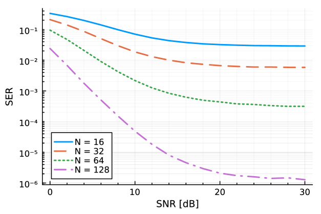
Figure 1: Monte Carlo results of the SER for the ML detector in terms of SNR. Various numbers of antennas have been considered under a correlated Rayleigh channel with $\rho=0.8$ (see Section V for a detailed model description).

II-D Energy detection and high SNR approximation

There is a special case of the ML problem presented in (6) which has been widely studied in the literature [5, 15]: the isotropic channel. Under this model, the spectral matrix $\boldsymbol{\Gamma}$ is proportional to the identity (i.e. $\boldsymbol{\Gamma}\triangleq\alpha\mathbf{I}_{N}$). This assumption greatly simplifies (10), since $\boldsymbol{\mathsf{r}}|x\sim\mathcal{CN}(\mathbf{0}_{N},(|x|^{2}\alpha+1)\mathbf{I}_{N})$:

$$\widehat{x}_{\mathrm{ML}}^{(\mathrm{iso})}=\arg\min_{x\in\mathcal{X}}\frac{\mathopen{}\mathclose{{}\left\|\mathbf{r}}\right\|^{2}}{|x|^{2}\alpha+1}+N\log\mathopen{}\mathclose{{}\left(|x|^{2}\alpha+1}\right).$$ (16)

In this scenario, $\|\mathbf{r}\|^{2}$ is a sufficient statistic [5].

Another relevant simplification of the ML detector that results in a similar expression arises at high SNR. Given a constellation $\mathcal{X}^{\prime}$ that does not include the null symbol $x=0$, the covariance matrix of the received signal reduces to

$$\lim_{\alpha\to\infty}\mathbf{C}_{\boldsymbol{\mathsf{r}}|x}=\lim_{\alpha\to\infty}|x|^{2}\mathbf{\Gamma},$$ (17)

with which detector (10) simplifies to

$$\lim_{\alpha\to\infty}\widehat{x}_{\mathrm{ML}}=\lim_{\alpha\to\infty}\operatorname*{arg\,min}_{x\in\mathcal{X}^{\prime}}\frac{\mathbf{r}^{\mathrm{H}}\mathbf{\Gamma}^{-1}\mathbf{r}}{|x|^{2}}+N\log\mathopen{}\mathclose{{}\left(|x|^{2}}\right)$$ (18)

and $\mathbf{r}^{\mathrm{H}}\mathbf{\Gamma}^{-1}\mathbf{r}$ becomes a sufficient statistic. This result is no longer valid for the constellation considered in (7), as $\mathbf{C}_{\boldsymbol{\mathsf{r}}|x=0}=\mathbf{I}_{N}$, so this symbol has to be treated separately to perform ML detection.

In both special cases (16) and (18), the ML decoder can be decoupled into a two-stage process:

1. The computation of a quadratic statistic.

2. A one-dimensional decision problem that detects the transmitted symbol solely using the proposed statistic.

Motivated by this observation, a generalization of this two-step approach for arbitrary channel and noise spectra is proposed in the sequel. Although, in general, ML detection cannot be decoupled in this manner, the two-step approach provides the appealing advantage of exhibiting a fixed complexity, i.e. not dependent on the constellation size $M$. Sections III and IV address the design of the first and second steps of this procedure.

III Energy statistic

The first simplified receiver described in Section II-D, known as ED, is widely used in the literature due to its low complexity and optimality within the isotropic channel. Nevertheless, when the channel is arbitrarily correlated, the ED does not fully exploit the statistical CSI and is no longer optimal. In this paper, we present a one-dimensional detector that incorporates channel correlation, while having a complexity that does not depend on the constellation size. We have chosen a quadratic structure (in data) of the form

$$\widehat{\varepsilon}\mathopen{}\mathclose{{}\left(\mathbf{r}}\right)\triangleq\mathbf{r}^{\mathrm{H}}\mathbf{A}\mathbf{r}+\mathbf{b}^{\mathrm{H}}\mathbf{r}+c,$$ (19)

as it generalizes the one for ED and is adequate when dealing with variables related to second order moments (such as transmitted energy $|x|^{2}$, in which we convey information). Its design is split into two phases: (i) we perform the energy estimation with (19) and then (ii) detect the transmitted symbol by classifying the estimate according to some detection regions.

Throughout this section, we consider the received signal from (9), $\boldsymbol{\mathsf{r}}|\varepsilon\sim\mathcal{CN}(\mathbf{0}_{N},\mathbf{C}_{\boldsymbol{\mathsf{r}}|\varepsilon}\triangleq\varepsilon\mathbf{\Gamma}+\mathbf{I}_{N})$, with transmitted energy $\varepsilon=|x|^{2}$.

III-A Information-theoretic design criteria

The detector based on expression (19) is suboptimal for most scenarios because $\widehat{\varepsilon}$ is not a sufficient statistic in the general case. Nevertheless, we wish to design the coefficients of the quadratic estimator so that it preserves as much information as possible on the transmitted symbol, so that the error rate performance penalty is minimized. Hence, the mutual information arises as a natural choice for the design criterion the coefficients of the quadratic estimator.

We propose to design coefficients $\mathbf{A},\mathbf{b},c$ to maximize the mutual information (MI)between the transmitted symbol and the estimator output, i.e.

$$\mathrm{I}\mathopen{}\mathclose{{}\left(\varepsilon;\widehat{\varepsilon}}\right)=\mathrm{h}\mathopen{}\mathclose{{}\left(\varepsilon}\right)-\mathrm{h}\mathopen{}\mathclose{{}\left(\varepsilon|\widehat{\varepsilon}}\right)\implies\widehat{\varepsilon}_{\mathrm{OPT}}\triangleq\arg\max_{\widehat{\varepsilon}\in\mathcal{Q}}\mathrm{I}\mathopen{}\mathclose{{}\left(\varepsilon;\widehat{\varepsilon}}\right),$$ (20)

where $\mathcal{Q}$ is the set of all estimators of the form (19). This problem is, in general, very hard to solve analytically. Motivated by [24], we obtain a lower bound on the MI:

$$\mathrm{I}\mathopen{}\mathclose{{}\left(\varepsilon;\widehat{\varepsilon}}\right) =\mathrm{h}\mathopen{}\mathclose{{}\left(\varepsilon}\right)-\mathrm{h}\mathopen{}\mathclose{{}\left(\varepsilon-\widehat{\varepsilon}|\widehat{\varepsilon}}\right)$$ (21)

$$\geq\mathrm{h}\mathopen{}\mathclose{{}\left(\varepsilon}\right)-\mathrm{h}\mathopen{}\mathclose{{}\left(\varepsilon-\widehat{\varepsilon}}\right).$$ (22)

Equality (21) is due to the translation invariance of differential entropy [25, Thm. 8.6.3], while inequality (22) is due to [25, Thm. 8.6.1]. If $\xi\triangleq\varepsilon-\widehat{\varepsilon}$ is interpreted as the estimation error, this lower bound will become tighter the less $\xi$ depends on $\widehat{\varepsilon}$, i.e. the better the estimation becomes.

By using the maximum value of $\mathrm{h}(\xi)$, which is achieved when $\xi$ is Gaussian [25, Thm. 8.6.5], an even simpler lower bound is derived:

$$\mathrm{I}\mathopen{}\mathclose{{}\left(\varepsilon;\widehat{\varepsilon}}\right)\geq\mathrm{h}\mathopen{}\mathclose{{}\left(\varepsilon}\right)-\frac{1}{2}\mathopen{}\mathclose{{}\left(1+\log\mathopen{}\mathclose{{}\left(2\pi\mathrm{var}(\xi)}\right)}\right)\triangleq\mathrm{I}_{\mathrm{LOW}}.$$ (23)

Therefore, the proposed design criterion simplifies to

$$\widehat{\varepsilon}=\arg\max_{\widehat{\varepsilon}\in\mathcal{Q}}\mathrm{I}_{\mathrm{LOW}}\equiv\arg\min_{\widehat{\varepsilon}\in\mathcal{Q}}\mathrm{var}(\xi).$$ (24)

This variance can be obtained from the average MSE and bias of $\widehat{\varepsilon}$, by applying the law of total expectation [26, Thm. 9.1.5]:

$$\mathrm{var}(\xi) =\operatorname{\mathrm{MSE}}\mathopen{}\mathclose{{}\left(\widehat{\varepsilon}}\right)-\operatorname{\mathrm{b}}^{2}\mathopen{}\mathclose{{}\left(\widehat{\varepsilon}}\right)$$ (25)

$$=\mathrm{E}_{\varepsilon}\mathopen{}\mathclose{{}\left[\mathrm{E}_{\boldsymbol{\mathsf{r}}|\varepsilon}\mathopen{}\mathclose{{}\left[\mathopen{}\mathclose{{}\left(\varepsilon-\widehat{\varepsilon}}\right)^{2}}\right]}\right]-\mathrm{E}_{\varepsilon}\mathopen{}\mathclose{{}\left[\varepsilon-\mathrm{E}_{\boldsymbol{\mathsf{r}}|\varepsilon}\mathopen{}\mathclose{{}\left[\widehat{\varepsilon}}\right]}\right]^{2}.$$

III-B Best quadratic unbiased estimator (BQUE)

Before dealing with the full optimization problem, it is of conceptual interest to study a simpler version. Consider a genie-aided estimator that aims at minimizing $\mathrm{var}(\xi)$ but is aware of the exact transmitted energy $\varepsilon$. In such a scenario, (25) reduces to:

$$\mathrm{var}(\xi) =\mathrm{E}_{\boldsymbol{\mathsf{r}}|\varepsilon}\mathopen{}\mathclose{{}\left[(\varepsilon-\widehat{\varepsilon})^{2}}\right]-\mathopen{}\mathclose{{}\left(\varepsilon-\mathrm{E}_{\boldsymbol{\mathsf{r}}|\varepsilon}\mathopen{}\mathclose{{}\left[\widehat{\varepsilon}}\right]}\right)^{2}$$ (26)

$$=\mathrm{E}_{\boldsymbol{\mathsf{r}}|\varepsilon}\mathopen{}\mathclose{{}\left[\widehat{\varepsilon}^{2}}\right]-\mathrm{E}_{\boldsymbol{\mathsf{r}}|\varepsilon}\mathopen{}\mathclose{{}\left[\widehat{\varepsilon}}\right]^{2}\equiv\mathrm{var}(\widehat{\varepsilon}|\varepsilon).$$

It depends on the conditional first and second order moments of $\widehat{\varepsilon}$, which have been derived in Appendix -C:

$$\mathrm{E}_{\boldsymbol{\mathsf{r}}|\varepsilon}\mathopen{}\mathclose{{}\left[\widehat{\varepsilon}}\right] =\mathrm{tr}(\mathbf{A}\mathbf{C}_{\boldsymbol{\mathsf{r}}|\varepsilon})+c$$ (27)

$$\mathrm{E}_{\boldsymbol{\mathsf{r}}|\varepsilon}\mathopen{}\mathclose{{}\left[\widehat{\varepsilon}^{2}}\right] =\mathrm{tr}(\mathbf{A}^{2}\mathbf{C}_{\boldsymbol{\mathsf{r}}|\varepsilon}^{2})+\mathrm{tr}(\mathbf{A}\mathbf{C}_{\boldsymbol{\mathsf{r}}|\varepsilon})^{2}+2c\cdot\mathrm{tr}(\mathbf{A}\mathbf{C}_{\boldsymbol{\mathsf{r}}|\varepsilon})$$

$$\quad+\mathbf{b}^{\mathrm{H}}\mathbf{C}_{\boldsymbol{\mathsf{r}}|\varepsilon}\mathbf{b}+c^{2}.$$

Using them in (26), the conditional variance of $\widehat{\varepsilon}$ becomes

$$\mathrm{var}(\widehat{\varepsilon}|\varepsilon)=\|\mathbf{A}\mathbf{C}_{\boldsymbol{\mathsf{r}}|\varepsilon}\|_{\mathrm{F}}^{2}+\mathbf{b}^{\mathrm{H}}\mathbf{C}_{\boldsymbol{\mathsf{r}}|\varepsilon}\mathbf{b},$$ (28)

which does not depend on the affine term $c$, as expected.

As the affine term does not affect the variance we want to optimize, we can freely set it. For convenience, we propose to choose it to obtain a conditionally unbiased estimator, which translates into

$$\mathrm{E}_{\boldsymbol{\mathsf{r}}|\varepsilon}\mathopen{}\mathclose{{}\left[\widehat{\varepsilon}}\right] =\mathrm{tr}(\mathbf{A}(\varepsilon\mathbf{\Gamma}+\mathbf{I}_{N}))+c=\varepsilon$$ (29)

$$\implies\begin{cases}c=-\mathrm{tr}\mathopen{}\mathclose{{}\left(\mathbf{A}}\right)\\ \mathrm{tr}\mathopen{}\mathclose{{}\left(\mathbf{A}\mathbf{\Gamma}}\right)=1.\end{cases}$$

Under conditional unbiasedness, $\mathrm{var}(\widehat{\varepsilon}|\varepsilon)$ is equivalent to the conditional MSE, i.e. $\operatorname{\mathrm{MSE}}(\widehat{\varepsilon}|\varepsilon)$. Following a similar reasoning to the one behind the best linear unbiased estimator (BLUE) [27, Ch. 6], with the quadratic structure presented, we will term the estimator that minimizes $\operatorname{\mathrm{MSE}}(\widehat{\varepsilon}|\varepsilon)$ best quadratic unbiased estimator (BQUE).

Accounting for the constraints in (29), we can solve the optimization problem using the method of Lagrange multipliers:

$$\mathcal{L}(\mathbf{A},\mathbf{b},\lambda)\triangleq\|\mathbf{A}\mathbf{C}_{\boldsymbol{\mathsf{r}}|\varepsilon}\|_{\mathrm{F}}^{2}+\mathbf{b}^{\mathrm{H}}\mathbf{C}_{\boldsymbol{\mathsf{r}}|\varepsilon}\mathbf{b}+\lambda\mathopen{}\mathclose{{}\left(\mathrm{tr}\mathopen{}\mathclose{{}\left(\mathbf{A}\mathbf{\Gamma}}\right)-1}\right).$$ (30)

We first differentiate $\mathcal{L}$ with respect to $\mathbf{b}$ and equate it to $\mathbf{0}$:

$$\frac{\partial\mathcal{L}(\mathbf{A},\mathbf{b},\lambda)}{\partial\mathbf{b}^{\mathrm{H}}}=\mathbf{C}_{\boldsymbol{\mathsf{r}}|\varepsilon}\mathbf{b}=\mathbf{0}_{N\times 1}\implies\mathbf{b}=\mathbf{0}_{N\times 1},$$ (31)

since $\mathbf{C}_{\boldsymbol{\mathsf{r}}|\varepsilon}$ is assumed full-rank. We can clearly see that $\widehat{\varepsilon}$ does not have a linear term. Then, regarding $\mathbf{A}$,

$$\frac{\partial\mathcal{L}(\mathbf{A},\lambda)}{\partial\mathbf{A}} =2\mathbf{C}_{\boldsymbol{\mathsf{r}}|\varepsilon}\mathbf{A}\mathbf{C}_{\boldsymbol{\mathsf{r}}|\varepsilon}+\lambda\mathbf{\Gamma}=\mathbf{0}_{N\times N}$$ (32)

$$\implies\mathbf{A}=-\frac{\lambda}{2}\mathbf{C}_{\boldsymbol{\mathsf{r}}|\varepsilon}^{-1}\mathbf{\Gamma}\mathbf{C}_{\boldsymbol{\mathsf{r}}|\varepsilon}^{-1}.$$

Taking into account that $\mathbf{\Gamma}$ and $\mathbf{C}_{\boldsymbol{\mathsf{r}}|\varepsilon}$ are diagonal matrices, $\mathbf{A}$ must also be diagonal. Enforcing the unbiasedness constraint leaves us with:

$$\mathrm{tr}\mathopen{}\mathclose{{}\left(\mathbf{A}\mathbf{\Gamma}}\right) =-\frac{\lambda}{2}\|\mathbf{\Gamma}\mathbf{C}_{\boldsymbol{\mathsf{r}}|\varepsilon}^{-1}\|_{\mathrm{F}}^{2}=1$$ (33)

$$\implies-\frac{\lambda}{2}=\frac{1}{\|\mathbf{\Gamma}\mathbf{C}_{\boldsymbol{\mathsf{r}}|\varepsilon}^{-1}\|_{\mathrm{F}}^{2}}.$$

Substituting in (32) we obtain the matrix of the quadratic form:

$$\mathbf{A}_{\mathrm{BQUE}}=\frac{\mathbf{\Gamma}\mathbf{C}_{\boldsymbol{\mathsf{r}}|\varepsilon}^{-2}}{\|\mathbf{\Gamma}\mathbf{C}_{\boldsymbol{\mathsf{r}}|\varepsilon}^{-1}\|_{\mathrm{F}}^{2}}.$$ (34)

Finally, the BQUE is given by

$$\widehat{\varepsilon}_{\mathrm{BQUE}}(\mathbf{r})=\frac{\mathbf{r}^{\mathrm{H}}\mathbf{\Gamma}\mathbf{C}_{\boldsymbol{\mathsf{r}}|\varepsilon}^{-2}\mathbf{r}-\mathrm{tr}(\mathbf{\Gamma}\mathbf{C}_{\boldsymbol{\mathsf{r}}|\varepsilon}^{-2})}{\|\mathbf{\Gamma}\mathbf{C}_{\boldsymbol{\mathsf{r}}|\varepsilon}^{-1}\|_{\mathrm{F}}^{2}}.$$ (35)

If we analyse the conditional MSE of this estimator, i.e.

$$\operatorname{\mathrm{MSE}}(\widehat{\varepsilon}_{\mathrm{BQUE}}|\varepsilon) =\|\mathbf{A}_{\mathrm{BQUE}}\mathbf{C}_{\boldsymbol{\mathsf{r}}|\varepsilon}\|_{\mathrm{F}}^{2}$$ (36)

$$=\frac{\|\mathbf{\Gamma}\mathbf{C}_{\boldsymbol{\mathsf{r}}|\varepsilon}^{-1}\|_{\mathrm{F}}^{2}}{\|\mathbf{\Gamma}\mathbf{C}_{\boldsymbol{\mathsf{r}}|\varepsilon}^{-1}\|_{\mathrm{F}}^{4}}=\frac{1}{\|\mathbf{\Gamma}\mathbf{C}_{\boldsymbol{\mathsf{r}}|\varepsilon}^{-1}\|_{\mathrm{F}}^{2}},$$

we observe it coincides with the CRB associated with the estimation of $\varepsilon$, which has been derived in Appendix -D. Although this condition is sufficient to state if an estimator is efficient, the BQUE depends on the parameter to be estimated, making it unrealizable. Therefore, it is not the MVUE [27, Ch. 2].

III-C QMMSE estimator

Developing the BQUE has provided us with valuable insights on problem (24) from the perspective of classical estimation theory. We now derive the structure of the quadratic estimator that maximizes $\mathrm{I}_{\mathrm{LOW}}$. Recall (25), which depends on the average MSE and squared mean bias of $\widehat{\varepsilon}$:

$$\operatorname{\mathrm{MSE}}\mathopen{}\mathclose{{}\left(\widehat{\varepsilon}}\right) =\mathrm{E}_{\varepsilon}\mathopen{}\mathclose{{}\left[\varepsilon^{2}-2\varepsilon\mathrm{E}_{\boldsymbol{\mathsf{r}}|\varepsilon}\mathopen{}\mathclose{{}\left[\widehat{\varepsilon}}\right]+\mathrm{E}_{\boldsymbol{\mathsf{r}}|\varepsilon}\mathopen{}\mathclose{{}\left[\widehat{\varepsilon}^{2}}\right]}\right]$$ (37)

$$\operatorname{\mathrm{b}}^{2}\mathopen{}\mathclose{{}\left(\widehat{\varepsilon}}\right) =1-2\mathrm{E}_{\varepsilon}\mathopen{}\mathclose{{}\left[\varepsilon\mathrm{E}_{\boldsymbol{\mathsf{r}}|\varepsilon}\mathopen{}\mathclose{{}\left[\widehat{\varepsilon}}\right]}\right]+\mathrm{E}_{\varepsilon}\mathopen{}\mathclose{{}\left[\mathrm{E}_{\boldsymbol{\mathsf{r}}|\varepsilon}\mathopen{}\mathclose{{}\left[\widehat{\varepsilon}}\right]}\right]^{2}.$$

Plugging the first and second-order moments from (27) in the previous expressions yields

$$\operatorname{\mathrm{MSE}}\mathopen{}\mathclose{{}\left(\widehat{\varepsilon}}\right) =\mathopen{}\mathclose{{}\left(c+\mathrm{tr}(\mathbf{A}\overline{\mathbf{C}})-1}\right)^{2}+\sigma_{\varepsilon}^{2}\mathopen{}\mathclose{{}\left(1-\mathrm{tr}(\mathbf{A}\mathbf{\Gamma})}\right)^{2}$$ (38)

$$\quad+\mathbf{b}^{\mathrm{H}}\overline{\mathbf{C}}\mathbf{b}+\mathrm{tr}(\mathbf{A}^{2}\mathring{\mathbf{C}}^{2})$$

$$\operatorname{\mathrm{b}}^{2}\mathopen{}\mathclose{{}\left(\widehat{\varepsilon}}\right) =\mathopen{}\mathclose{{}\left(c+\mathrm{tr}(\mathbf{A}\overline{\mathbf{C}})-1}\right)^{2},$$

with $\overline{\mathbf{C}}\triangleq\mathbf{\Gamma}+\mathbf{I}_{N}$, $\mathring{\mathbf{C}}^{2}\triangleq(\sigma_{\varepsilon}^{2}+1)\mathbf{\Gamma}^{2}+2\mathbf{\Gamma}+\mathbf{I}_{N}$ and $\sigma_{\varepsilon}^{2}\triangleq\mathrm{var}(\varepsilon)$. Therefore, the variance to be minimized results in

$$\mathrm{var}(\xi)=\sigma_{\varepsilon}^{2}\mathopen{}\mathclose{{}\left(1-\mathrm{tr}(\mathbf{A}\mathbf{\Gamma})}\right)^{2}+\mathbf{b}^{\mathrm{H}}\overline{\mathbf{C}}\mathbf{b}+\|\mathbf{A}\mathring{\mathbf{C}}\|_{\mathrm{F}}^{2},$$ (39)

which is not affected by the value of $c$, similar to what occurred with the BQUE. If we set it to $c\triangleq 1-\mathrm{tr}(\mathbf{A}\overline{\mathbf{C}})$, the squared mean bias term cancels (i.e. $\operatorname{\mathrm{b}}^{2}(\widehat{\varepsilon})=0$). In this situation, the criterion of maximum $\mathrm{I}_{\mathrm{LOW}}$ is equivalent to that of minimum MSE on average. This results in the (Bayesian) QMMSE estimator, which is an extension of the well-known linear minimum mean squared error (LMMSE)estimator [27, Ch. 12].

To obtain its expression, we shall proceed as in Section III-B, by differentiating (39) and equating it to $\mathbf{0}$. The linear term $\mathbf{b}$ is $\mathbf{0}_{N\times 1}$ straightforwardly, due to the rank-completeness of $\overline{\mathbf{C}}$. As for the matrix in the quadratic term,

$$\frac{\partial\mathrm{var}(\xi)}{\partial\mathbf{A}}=-2\sigma_{\varepsilon}^{2}\mathopen{}\mathclose{{}\left(1-\mathrm{tr}(\mathbf{A}\mathbf{\Gamma})}\right)\mathbf{\Gamma}+2\mathbf{A}\mathring{\mathbf{C}}^{2}=\mathbf{0}_{N\times N}.$$ (40)

By isolating $\mathbf{A}$, multiplying it by $\mathbf{\Gamma}$ and computing the trace, we obtain the following term:

$$\mathrm{tr}(\mathbf{A\Gamma})=\frac{\sigma_{\varepsilon}^{2}\|\mathbf{\Gamma}\mathring{\mathbf{C}}^{-1}\|_{\mathrm{F}}^{2}}{1+\sigma_{\varepsilon}^{2}\|\mathbf{\Gamma}\mathring{\mathbf{C}}^{-1}\|_{\mathrm{F}}^{2}},$$ (41)

which yields the matrix

$$\mathbf{A}_{\mathrm{QMMSE}}=\frac{\sigma_{\varepsilon}^{2}\mathbf{\Gamma}\mathring{\mathbf{C}}^{-2}}{1+\sigma_{\varepsilon}^{2}\|\mathbf{\Gamma}\mathring{\mathbf{C}}^{-1}\|_{\mathrm{F}}^{2}}$$ (42)

and the estimator

$$\widehat{\varepsilon}_{\mathrm{QMMSE}}(\mathbf{r})=\frac{\sigma_{\varepsilon}^{2}\mathbf{r}^{\mathrm{H}}\mathbf{\Gamma}\mathring{\mathbf{C}}^{-2}\mathbf{r}+1-\sigma_{\varepsilon}^{2}\mathrm{tr}(\mathbf{\Gamma}\mathring{\mathbf{C}}^{-2})}{1+\sigma_{\varepsilon}^{2}\|\mathbf{\Gamma}\mathring{\mathbf{C}}^{-1}\|_{\mathrm{F}}^{2}}.$$ (43)

The mean MSE value it reaches is

$$\operatorname{\mathrm{MSE}}(\widehat{\varepsilon}_{\mathrm{QMMSE}})=\frac{\sigma_{\varepsilon}^{2}}{1+\sigma_{\varepsilon}^{2}\|\mathbf{\Gamma}\mathring{\mathbf{C}}^{-1}\|_{\mathrm{F}}^{2}}.$$ (44)

III-D Unified framework for quadratic detectors

As stated in Section II-D, the general framework outlined in (19) is general enough to encapsulate a variety of energy estimators as a first step in symbol detection. For instance, an estimator of the form

$$\mathbf{A}_{\mathrm{ED}}\triangleq\frac{\mathbf{I}_{N}}{\mathrm{tr}\mathopen{}\mathclose{{}\left(\mathbf{\Gamma}}\right)}\implies\widehat{\varepsilon}_{\mathrm{ED}}(\mathbf{r})=\frac{\|\mathbf{r}\|^{2}-N}{\mathrm{tr}\mathopen{}\mathclose{{}\left(\mathbf{\Gamma}}\right)}$$ (45)

with a posterior classification (with suitable decision regions) is equivalent to the energy detector from (16). Similarly, for the high SNR detector in (18), its corresponding quadratic statistic is

$$\mathbf{A}_{\mathrm{HSNR}}\triangleq\frac{\mathbf{\Gamma}^{-1}}{N}\implies\widehat{\varepsilon}_{\mathrm{HSNR}}(\mathbf{r})=\frac{\mathbf{r}^{\mathrm{H}}\mathbf{\Gamma}^{-1}\mathbf{r}-\mathrm{tr}(\mathbf{\Gamma}^{-1})}{N}.$$ (46)

Notice that the affine term in both cases has been set to $c=1-\mathrm{tr}(\mathbf{A}\overline{\mathbf{C}})$ to more easily compare them with the QMMSE. Remarkably, this makes them conditionally unbiased.

An interesting aspect regarding $\widehat{\varepsilon}_{\mathrm{QMMSE}}$ is that, in the high SNR regime, its quadratic term matrix becomes

$$\lim_{\alpha\to\infty}\mathbf{A}_{\mathrm{QMMSE}}=\lim_{\alpha\to\infty}\frac{1}{1+\frac{1}{\sigma_{\varepsilon}^{2}}+N}\mathbf{\Gamma}^{-1}.$$ (47)

This is a scaled version of $\mathbf{A}_{\mathrm{HSNR}}$ and, in fact, both matrices coincide for asymptotically large $N$. Therefore, at high SNR, both $\widehat{\varepsilon}_{\mathrm{QMMSE}}$ and $\widehat{\varepsilon}_{\mathrm{HSNR}}$ will present the same performance and error floor.

Another important property of $\widehat{\varepsilon}_{\mathrm{ED}}$, $\widehat{\varepsilon}_{\mathrm{HSNR}}$ and $\widehat{\varepsilon}_{\mathrm{BQUE}}$ is that they all converge to the same estimator when the channel is assumed to be isotropic:

$$\widehat{\varepsilon}(\mathbf{r})=\frac{1}{\alpha}\mathopen{}\mathclose{{}\left(\frac{1}{N}\|\mathbf{r}\|^{2}-1}\right).$$ (48)

Similarly, $\widehat{\varepsilon}_{\mathrm{QMMSE}}$ becomes

$$\widehat{\varepsilon}^{\prime}(\mathbf{r})=\frac{\|\mathbf{r}\|^{2}+\frac{(\alpha+1)^{2}}{\sigma_{\varepsilon}^{2}\alpha}+\alpha-N}{\frac{(\alpha+1)^{2}}{\sigma_{\varepsilon}^{2}\alpha}+\alpha+N\alpha},$$ (49)

which is a scaled and translated version of (48), i.e. they define equivalent detectors with appropriate decision regions.

IV Symbol detection

Once the energy estimation phase has been studied, we now move on to the second step in the architecture proposed in Section III: symbol detection. For a given constellation, we describe the detection regions considering that the energy statistic asymptotically follows a Gaussian distribution. Afterwards, we analyse the probability of error of quadratic detectors and present a decision-directed design that leverages the BQUE to provide an improved performance.

IV-A Detection regions

Quadratic energy estimators of the form (19) (ignoring the linear term which is zero) can be expressed as a summation:

$$\widehat{\varepsilon}\mathopen{}\mathclose{{}\left(\mathbf{r}}\right)=\mathbf{r}^{\mathrm{H}}\mathbf{A}\mathbf{r}+c=\sum\limits_{n=1}^{N}a_{n}\mathopen{}\mathclose{{}\left|r_{n}}\right|^{2}+c_{n},$$ (50)

where $a_{n}\triangleq[\mathbf{A}]_{n,n}$ and $\sum_{n}c_{n}\triangleq c$. Particularizing for the estimators presented in the previous section, we can set $c\triangleq 1-\mathrm{tr}(\mathbf{A}(\mathbf{\Gamma}+\mathbf{I}_{N}))$. Notice how (50) produces a real output. Therefore, defining a decision region $\mathcal{R}_{x}$ for each $x\in\mathcal{X}$ consists in determining detection thresholds on the real line:

$$\widehat{x}=\begin{cases}x_{1},\quad&\widehat{\varepsilon}\leq\tau_{1},\\ x_{i},\quad&\tau_{i-1}<\widehat{\varepsilon}<\tau_{i},\\ x_{M},\quad&\tau_{M-1}\leq\widehat{\varepsilon}.\end{cases}$$ (51)

The thresholds that minimize the error probability, $\mathcal{T}\triangleq\{\tau_{i}\}_{1\leq i\leq M-1}$, are found at the intersection between the densities of the estimator output conditioned to every transmitted symbol of $\mathcal{X}$.

Since $\widehat{\varepsilon}(\boldsymbol{\mathsf{r}}|\varepsilon)$ is a quadratic form of a complex normal vector, it has a generalized chi-squared distribution [29]. Its PDF can be obtained analytically in specific cases, such as in [15], where the authors derive it for the ED under the exponential correlation channel (see Section V). Nevertheless, the resulting expressions for general quadratic detectors and arbitrary correlation models are usually very involved [30, Ch. 1], [31] and do not allow for a simple derivation of detection thresholds.

In the context of massive SIMO, we can exploit the asymptotic properties of $\widehat{\varepsilon}(\boldsymbol{\mathsf{r}}|\varepsilon)$ for a large $N$. Invoking the central limit theorem (CLT),

$$\widehat{\varepsilon}\mathopen{}\mathclose{{}\left(\boldsymbol{\mathsf{r}}|\varepsilon}\right)\xrightarrow{\mathrm{d}}\mathcal{N}\mathopen{}\mathclose{{}\left(1-(1-\varepsilon)\mathrm{tr}\mathopen{}\mathclose{{}\left(\mathbf{A}\mathbf{\Gamma}}\right),\,\mathopen{}\mathclose{{}\left\|\mathbf{A}\mathopen{}\mathclose{{}\left(\varepsilon\mathbf{\Gamma}+\mathbf{I}_{N}}\right)}\right\|_{\mathrm{F}}^{2}}\right),$$ (52)

as $N\to\infty$. For the unbiased estimators, $\mathrm{tr}\mathopen{}\mathclose{{}\left(\mathbf{A}\mathbf{\Gamma}}\right)=1$, thus the Gaussian density function is centered at the symbol energy level. Observe that the terms in sum (50) are independent but not identically distributed. To ensure the CLT can be applied in this scenario, it is sufficient to prove that Lyapunov’s condition is satisfied. In Appendix -E we show that it does indeed hold, thus validating the use of the CLT. This result motivates employing a Gaussian approximation for the densities of $\widehat{\varepsilon}(\boldsymbol{\mathsf{r}}|\varepsilon)$ which, on its turn, implies that the bound in Eq. (23) is asymptotically an equality.

In the Gaussian case, finding the intersection points reduces to finding the roots of a second-degree polynomial for each pair of adjacent densities. In general, each polynomial has two roots, but we are only interested in the one between the two likelihoods. Taking into account that the variance increases when the symbol energy does as well, we conclude that the desired root is the greatest one, thus the maximum of each pair must be taken to find the thresholds. This procedure is summarized in Algorithm 1.

Algorithm 1 Thresholds between Gaussian Likelihoods

1:constellation $\mathcal{X}$, matrix $\mathbf{A}$, spectrum $\mathbf{\Gamma}$

2:thresholds $\mathcal{T}=\mathopen{}\mathclose{{}\left\{\tau_{1},\dots,\tau_{M-1}}\right\}$

3:procedure NormalIntersection($\mu_{1},\mu_{2},\sigma^{2}_{1},\sigma^{2}_{2}$)

4:     $a=1/\sigma^{2}_{2}-1/\sigma^{2}_{1}$

5:     $b=2\cdot(\mu_{1}/\sigma^{2}_{1}-\mu_{2}/\sigma^{2}_{2})$

6:     $c=\mu_{2}^{2}/\sigma^{2}_{2}-\mu_{1}^{2}/\sigma^{2}_{1}+\log(\sigma^{2}_{2}/\sigma^{2}_{1})$

7:     return $\mathrm{roots}(\mathcal{P}(c,b,a))$

8:end procedure

9:for $i=1:M-1$ do

10:     $\mu_{1}=1-\mathopen{}\mathclose{{}\left(1-\varepsilon_{i}}\right)\mathrm{tr}\mathopen{}\mathclose{{}\left(\mathbf{A\Gamma}}\right)$

11:     $\mu_{2}=1-\mathopen{}\mathclose{{}\left(1-\varepsilon_{i+1}}\right)\mathrm{tr}\mathopen{}\mathclose{{}\left(\mathbf{A\Gamma}}\right)$

12:     $\sigma^{2}_{1}=\mathrm{tr}\mathopen{}\mathclose{{}\left(\mathbf{A}^{2}(\varepsilon_{i}\mathbf{\Gamma}+\mathbf{I}_{N})^{2}}\right)$

13:     $\sigma^{2}_{2}=\mathrm{tr}\mathopen{}\mathclose{{}\left(\mathbf{A}^{2}(\varepsilon_{i+1}\mathbf{\Gamma}+\mathbf{I}_{N})^{2}}\right)$

14:     $\tau_{i}=\max(\textsc{NormalIntersection}(\mu_{1},\mu_{2},\sigma^{2}_{1},\sigma^{2}_{2}))$

15:end for

16:return $\mathcal{T}$

IV-B Probability of detection error

From (51) we observe that the error probability can be computed as:

$$\mathrm{P}_{\epsilon} =\frac{1}{M}\bigg{(}\mathrm{Pr}\mathopen{}\mathclose{{}\left[\widehat{\varepsilon}(\boldsymbol{\mathsf{r}}|\varepsilon_{1})>\tau_{1}}\right]+\mathrm{Pr}\mathopen{}\mathclose{{}\left[\widehat{\varepsilon}(\boldsymbol{\mathsf{r}}|\varepsilon_{M})<\tau_{M-1}}\right]$$ (53)

$$\quad+\sum_{i=2}^{M-1}\mathrm{Pr}\mathopen{}\mathclose{{}\left[\widehat{\varepsilon}(\boldsymbol{\mathsf{r}}|\varepsilon_{i})<\tau_{i-1}}\right]+\mathrm{Pr}\mathopen{}\mathclose{{}\left[\widehat{\varepsilon}(\boldsymbol{\mathsf{r}}|\varepsilon_{i})>\tau_{i}}\right]\bigg{)}.$$

Under the Gaussian assumption, each tail probability is approximated with the $\mathrm{Q}$-function:

$$\mathrm{Pr}\mathopen{}\mathclose{{}\left[\widehat{\varepsilon}(\boldsymbol{\mathsf{r}}|\varepsilon_{i})<\tau_{i-1}}\right]\approx\mathrm{Q}\mathopen{}\mathclose{{}\left(\frac{1-(1-\varepsilon_{i})\mathrm{tr}\mathopen{}\mathclose{{}\left(\mathbf{A}\mathbf{\Gamma}}\right)-\tau_{i-1}}{\mathopen{}\mathclose{{}\left\|\mathbf{A}\mathopen{}\mathclose{{}\left(\varepsilon_{i}\boldsymbol{\Gamma}+\mathbf{I}_{N}}\right)}\right\|_{\mathrm{F}}}}\right)$$

$$\mathrm{Pr}\mathopen{}\mathclose{{}\left[\widehat{\varepsilon}(\boldsymbol{\mathsf{r}}|\varepsilon_{i})>\tau_{i}}\right]\approx\mathrm{Q}\mathopen{}\mathclose{{}\left(\frac{\tau_{i}-1+(1-\varepsilon_{i})\mathrm{tr}\mathopen{}\mathclose{{}\left(\mathbf{A}\mathbf{\Gamma}}\right)}{\mathopen{}\mathclose{{}\left\|\mathbf{A}\mathopen{}\mathclose{{}\left(\varepsilon_{i}\boldsymbol{\Gamma}+\mathbf{I}_{N}}\right)}\right\|_{\mathrm{F}}}}\right),$$ (54)

with $\varepsilon_{i}$ defined as in (7). Thus, the error probability is approximately given by:

$$\mathrm{P}_{\epsilon} \approx\frac{1}{M}\Bigg{(}\sum_{i=2}^{M}\mathrm{Q}\bigg{(}\frac{1-(1-\varepsilon_{i})\mathrm{tr}\mathopen{}\mathclose{{}\left(\mathbf{A}\mathbf{\Gamma}}\right)-\tau_{i-1}}{\mathopen{}\mathclose{{}\left\|\mathbf{A}\mathopen{}\mathclose{{}\left(\varepsilon_{i}\boldsymbol{\Gamma}+\mathbf{I}_{N}}\right)}\right\|_{\mathrm{F}}}\bigg{)}$$ (55)

$$\quad+\sum_{j=1}^{M-1}\mathrm{Q}\bigg{(}\frac{\tau_{j}-1+(1-\varepsilon_{j})\mathrm{tr}\mathopen{}\mathclose{{}\left(\mathbf{A}\mathbf{\Gamma}}\right)}{\mathopen{}\mathclose{{}\left\|\mathbf{A}\mathopen{}\mathclose{{}\left(\varepsilon_{j}\boldsymbol{\Gamma}+\mathbf{I}_{N}}\right)}\right\|_{\mathrm{F}}}\bigg{)}\Bigg{)}.$$

In expression (55) we observe that the error probability increases with the norms $\|\mathbf{A}(\varepsilon_{j}\boldsymbol{\Gamma}+\mathbf{I}_{N})\|_{\mathrm{F}}$, which correspond to the MSE of the BQUE for each symbol. This dependence shows that the information-theoretic criteria proposed in III-A is indeed justified. Nevertheless, optimizing MSE on average (i.e. as in QMMSE) is not consistent with the fact that the PEP of each symbol has a different effect on the error probability for each SNR level.

IV-C Assisted BQUE (ABQUE)

In order to overcome the previous issue, we now propose to assist the BQUE by replacing the true transmitted symbol known by the genie-aided decoder by the final decision delivered by the ED. By doing so, we build a hard-decision detector which exhibits some computational advantages compared with its soft alternative (plugging the energy estimation without deciding). On the one hand, assisting with hard decisions is prone to error boosting at low-SNR. However, the simulations in Section V will show that this effect is negligible except for extremely high antenna correlation. On the other hand, in the hard-decision scheme, the symbol plugged into the BQUE belongs to a known constellation, thus matrices $\mathbf{A}_{\mathrm{BQUE},\,i}$ for each symbol only need to be computed once and can be stored for later uses:

$$\mathbf{A}_{\mathrm{BQUE},\,i}=\frac{\mathbf{\Gamma}\mathbf{C}_{\boldsymbol{\mathsf{r}}|\varepsilon_{i}}^{-2}}{\|\mathbf{\Gamma}\mathbf{C}_{\boldsymbol{\mathsf{r}}|\varepsilon_{i}}^{-1}\|_{\mathrm{F}}^{2}},\quad 1\leq i\leq M.$$ (56)

This result has further implications. Given that the thresholds of the proposed quadratic detectors only depend on the constellation and $\mathbf{A}$, if $\mathbf{A}$ can be computed only once, thresholds can also be computed only once.

The major drawback of ABQUE is that an analytic expression of its error probability is difficult to obtain. However, simulations show that, for channels with low or moderate correlation, its performance is very close to that of BQUE. Therefore, the error probability expression of the latter can be used as an approximation for the former in various scenarios.

V Numerical results

In this section, we numerically validate the theoretical results presented in the previous sections and compare the various detectors in terms of the average SER performance. Analytical expressions predicting the error rate performance (continuous lines) of the high SNR, ED, QMMSE and BQUE detectors are compared with Monte Carlo method results (lines with markers) in the figures below. In all simulations we have employed the signal model (1) assuming the exponential correlation channel model described in [13]:

$$[\mathbf{C}_{\boldsymbol{\mathsf{h}}}]_{k,l}=c_{k,l}=\begin{cases}\rho^{l-k},\quad k\leq l,\\ c_{l,k}^{*},\quad k>l,\end{cases}$$ (57)

with correlation coefficient $\rho=0.7$ (unless stated otherwise). Symbols from a uniform unipolar 8-ASK constellation have been transmitted with average power equal to one. We have chosen a standard constellation instead of one optimized to the channel statistics (e.g. see [13]) to better portray a realistic scenario, with a low complexity transmitter that is unaware of CSI. It has the added benefit of being robust to SNR estimation errors in transmission.

In Fig. 2, the performance of all detectors discussed previously is depicted as a function of the SNR for $N=512$ antennas. We have computed the thresholds for each quadratic detector and then classified the estimated powers, as described in Section IV-A. The most remarkable outcome is that the ABQUE exhibits a performance very close to that of the oracle (i.e. BQUE) with just a narrow increase in complexity. Note that the ED error floor is much higher than that of the other quadratic detectors, which share it with the genie-aided detector. This error floor is very close to the one obtained with ML detection. The reason behind the slight discrepancy is that, although the CLT holds, the Gaussian likelihoods assumed in Algorithm 1 present inaccuracies that affect the threshold positioning, thus resulting in an increased error floor.

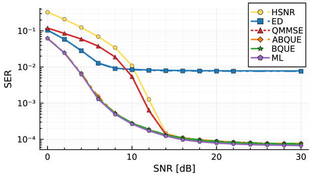
Figure 2: SER of the presented detectors in terms of SNR for $N=512$.

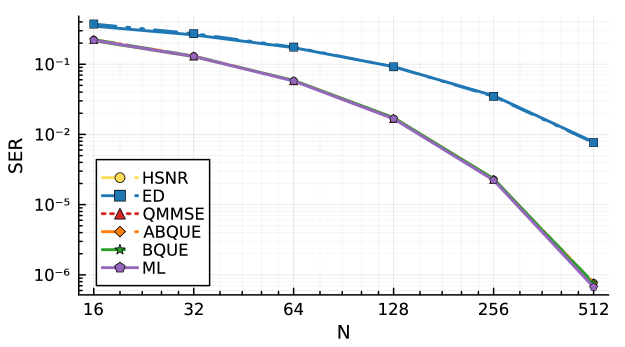
Figure 3: Floor level (i.e. SER at $\mathrm{SNR}=$30\text{\,}\mathrm{dB}$$) of the presented detectors in terms of $N$.

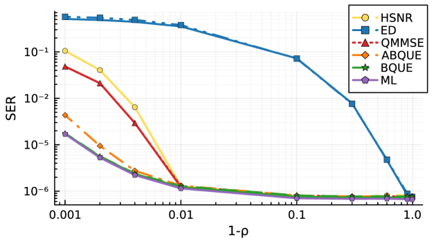
Figure 4: Floor level (i.e. SER at $\mathrm{SNR}=$30\text{\,}\mathrm{dB}$$) of the presented detectors in terms of channel correlation. The plot is with respect to $1-\rho$ for better visualization.

Figs. 3 and 4 illustrate the error floor level by depicting the SER of the different detectors at $\mathrm{SNR}=$30\text{\,}\mathrm{dB}$$ in terms of the number of antennas and the correlation coefficient, respectively. In the former, we can observe that the difference between the theoretical and the numerical SER is appreciable for small $N$, illustrating how the Gaussian approximation improves when the number of antennas increases. Regarding the error probability behavior in terms of channel correlation, it is worth to remark the robustness of QMMSE and ABQUE detectors, as for $0\leq\rho\leq 0.9$ the error floor does not change significantly. In addition, they share the SER with the ML detector for $\rho<0.99$ (up to the gap mentioned above). On the other hand, the error probability of the ED increases fast with the correlation. For instance, at $\rho=0.5$, it has grown more than 10 times compared with the no correlation case.

VI Conclusions

In this paper, we have analysed the fundamental limitations of one-shot SIMO noncoherent communication when an arbitrary PAM constellation is considered. We have also introduced a quadratic framework that generalizes the ED commonly used in the literature. We have derived an analytic approximation for the error probability of any detector exhibiting the quadratic structure proposed, as a sum of $\mathrm{Q}$-functions. An improved scheme based on the combination of quadratic detectors has also been presented. Its performance has been tested through several Monte Carlo experiments, as well as the validity of the SER approximations.

We can outline some future research lines that arise from this work. The most straightforward one is to design PAM constellations optimized for a particular quadratic detector, by means of minimizing the error probability approximation (55). Similar approaches are studied in [10, 4, 13]. Other potential extensions of the presented analysis include the design of codes across multiple channel uses and suitable detection schemes [32, 5]. Finally, a possible application of the proposed framework is in noncoherent energy detection of index modulations [33, 34]. For instance, considering a frequency selective channel and a multicarrier modulation such as orthogonal frequency division multiplexing (OFDM), information can be conveyed by assigning different transmission power levels to different sets of subcarriers.

-A Proof of Theorem 1

The PEP can be upper-bounded making use of Cantelli’s inequality [35]:

$$\mathrm{P}_{a\to b}\leq\mathopen{}\mathclose{{}\left(1+\Delta_{a,b}}\right)^{-1},$$ (58)

where

$$\Delta_{a,b}\triangleq\frac{\mathrm{E}_{\boldsymbol{\mathsf{r}}|x_{a}}\mathopen{}\mathclose{{}\left[\mathrm{L}_{a,b}\mathopen{}\mathclose{{}\left(\boldsymbol{\mathsf{r}}|x_{a}}\right)}\right]^{2}}{\mathrm{var}_{\boldsymbol{\mathsf{r}}|x_{a}}\mathopen{}\mathclose{{}\left(\mathrm{L}_{a,b}\mathopen{}\mathclose{{}\left(\boldsymbol{\mathsf{r}}|x_{a}}\right)}\right)}.$$ (59)

We must check whether this term grows without bounds, so that the PEP vanishes. This is intimately related to the channel hardening phenomenon exhibited by large arrays; notice how (59) is analogous to [36, Eq. 10].

The elements involved in the computation of (59) are:

$$\mathrm{E}_{\boldsymbol{\mathsf{r}}|x_{a}}\mathopen{}\mathclose{{}\left[\mathrm{L}_{a,b}\mathopen{}\mathclose{{}\left(\boldsymbol{\mathsf{r}}|x_{a}}\right)}\right]=\sum_{n=1}^{N}\mathopen{}\mathclose{{}\left(\lambda_{n}-1-\log\lambda_{n}}\right),$$ (60)

$$\mathrm{var}_{\boldsymbol{\mathsf{r}}|x_{a}}\mathopen{}\mathclose{{}\left(\mathrm{L}_{a,b}\mathopen{}\mathclose{{}\left(\boldsymbol{\mathsf{r}}|x_{a}}\right)}\right)=\sum_{n=1}^{N}\mathopen{}\mathclose{{}\left(\lambda_{n}-1}\right)^{2},$$

where

$$\lambda_{n}\triangleq\frac{|x_{a}|^{2}\gamma_{n}+1}{|x_{b}|^{2}\gamma_{n}+1}.$$ (61)

Thus, we are left with

$$\Delta_{a,b}=\frac{\mathopen{}\mathclose{{}\left(\sum_{n=1}^{N}\mathopen{}\mathclose{{}\left(\lambda_{n}-1-\log\lambda_{n}}\right)}\right)^{2}}{\sum_{n=1}^{N}\mathopen{}\mathclose{{}\left(\lambda_{n}-1}\right)^{2}}\triangleq\frac{u_{N}}{d_{N}}.$$ (62)

The proof is based on the Stolz-Cesàro theorem [37, Th. 2.7.2], so various requirements must be fulfilled to apply it. Both $\{u_{n}\}_{n\geq 1}$ and $\{d_{n}\}_{n\geq 1}$ are sequences of real numbers. In addition, $\{d_{n}\}_{n\geq 1}$ must be strictly monotone and divergent, which is guaranteed due to the test for divergence (i.e. the contrapositive of [37, Lemma 4.1.2]), by ensuring

$$(\lambda_{n}-1)^{2}>0,\quad\forall n\in\{1,\dots,\mathrm{\Theta}(N)\},$$ (63)

such that $\lim_{N\to\infty}\mathrm{\Theta}(N)=\infty$. This condition reduces to

$$\lambda_{n}\neq 1\iff|x_{a}|^{2}\gamma_{n}+1\neq|x_{b}|^{2}\gamma_{n}+1.$$ (64)

Thus, under the premise of the spectrum $\{\gamma_{n}\}_{n\geq 1}$ being nonnegative and bounded, our only requirement is

$$|x_{a}|^{2}\neq|x_{b}|^{2}\iff x_{a}\neq x_{b},\quad x_{a},x_{b}\in\mathcal{X},$$ (65)

which is consistent with the loss of phase information observed in the ML detector (6). This is a particular case of the principle of unique factorization [17, 38]. As it will be clear by the end of this proof, it is the minimum requirement for noncoherent constellations to allow for asymptotically error-free performance as the number of receiving antennas increases.

Having dealt with the behavior of $\{d_{n}\}_{n\geq 1}$, we are now in position to apply the Stolz-Cesàro theorem:

$$\lim_{N\to\infty}\Delta_{a,b} =\lim_{N\to\infty}\frac{u_{N+1}-u_{N}}{d_{N+1}-d_{N}}$$ (66)

$$=\lim_{N\to\infty}\frac{\eta\mathopen{}\mathclose{{}\left(\lambda_{N+1}}\right)\mathopen{}\mathclose{{}\left(\eta\mathopen{}\mathclose{{}\left(\lambda_{N+1}}\right)+2\sum\limits_{n=1}^{N}\eta\mathopen{}\mathclose{{}\left(\lambda_{n}}\right)}\right)}{\mathopen{}\mathclose{{}\left(\lambda_{N+1}-1}\right)^{2}},$$

where $\eta(x)\triangleq x-1-\log x$ is a nonnegative convex function that is 0 only at $x=1$. Each term involved in (66) is positive by property (65), and bounded due to the boundedness of $\{\gamma_{n}\}_{n\geq 1}$. Then, the previous limit simplifies to

$$\lim_{N\to\infty}\Delta_{a,b}=\lim_{N\to\infty}\frac{2\eta\mathopen{}\mathclose{{}\left(\lambda_{N+1}}\right)}{\mathopen{}\mathclose{{}\left(\lambda_{N+1}-1}\right)^{2}}\sum\limits_{n=1}^{N}\eta\mathopen{}\mathclose{{}\left(\lambda_{n}}\right),$$ (67)

which will grow without bounds since the test for divergence holds for the sum involved. This completes the proof. ∎

-B Proof of Theorem 2

Referring to (11), the PEP can be expressed as [23, Ch. 2.4]

$$\mathrm{P}_{a\to b}=\int_{\mathcal{D}}f_{\boldsymbol{\mathsf{r}}|x_{a}}(\mathbf{r})\operatorname{\mathrm{d}\!}\mathbf{r},$$ (68)

where $\mathcal{D}\triangleq\mathopen{}\mathclose{{}\left\{\mathbf{r}\in\mathbb{C}^{N}:f_{\boldsymbol{\mathsf{r}}|x_{b}}(\mathbf{r})\geq f_{\boldsymbol{\mathsf{r}}|x_{a}}(\mathbf{r})}\right\}$. With some simple manipulations, we can see that the boundary of this region defines an $(N-1)$-dimensional complex ellipsoid:

$$\partial\mathcal{D}=\mathopen{}\mathclose{{}\left\{\mathbf{r}\in\mathbb{C}^{N}:\mathbf{r}^{\mathrm{H}}\mathbf{K}\mathbf{r}=1}\right\},\,\,\mathbf{K}\triangleq\frac{\mathbf{C}_{\boldsymbol{\mathsf{r}}|x_{b}}^{-1}-\mathbf{C}_{\boldsymbol{\mathsf{r}}|x_{a}}^{-1}}{\log\bigl{|}\mathbf{C}_{\boldsymbol{\mathsf{r}}|x_{a}}\mathbf{C}_{\boldsymbol{\mathsf{r}}|x_{b}}^{-1}\bigr{|}}.$$ (69)

Without loss of generality, we assume the channel is full-rank (i.e. $\lambda_{n}>0$ for $n=1,\dots,N$). If condition (15) is fulfilled, $\mathbf{K}$ is always positive definite, ensuring the ellipsoid exists.

When $|x_{a}|^{2}>|x_{b}|^{2}$, $\mathcal{D}$ is the closure of the set of points inside ellipsoid (69). With a change of variable $\mathbf{r}\triangleq|\mathbf{K}|^{\frac{1}{2N}}\mathbf{K}^{-\frac{1}{2}}\mathbf{s}$, we can map it to a $N$-dimensional closed ball with the same volume:

$$\mathcal{D}\mapsto\mathcal{U}\triangleq\mathopen{}\mathclose{{}\left\{\mathbf{s}\in\mathbb{C}^{N}:\|\mathbf{s}\|^{2}\leq|\mathbf{K}|^{-\frac{1}{N}}}\right\}.$$ (70)

Then, the PEP becomes:

$$\mathrm{P}_{a\to b}=\int_{\mathcal{U}}\frac{\exp\mathopen{}\mathclose{{}\left(-\mathbf{s}^{\mathrm{H}}\mathbf{\Omega}^{-1}\mathbf{s}}\right)}{\pi^{N}|\mathbf{C}_{\boldsymbol{\mathsf{r}}|x_{a}}|}\operatorname{\mathrm{d}\!}\mathbf{s},\quad\mathbf{\Omega}\triangleq\frac{\mathbf{C}_{\boldsymbol{\mathsf{r}}|x_{a}}\mathbf{K}}{|\mathbf{K}|^{\frac{1}{N}}},$$ (71)

which is the integral of a multivariate complex Gaussian function. We can lower-bound it with the integral in $\mathcal{U}$ of a narrower Gaussian function that is tangent to it along the direction with the lowest eigenvalue of $\mathbf{\Omega}$, named $\underline{\omega}$. It is proportional to the PDF of $\boldsymbol{\mathsf{t}}\sim\mathcal{CN}(\mathbf{0}_{N},\underline{\omega}\mathbf{I}_{N})$:

$$\mathrm{P}_{a\to b}\geq\int_{\mathcal{U}}\frac{\exp\mathopen{}\mathclose{{}\left(-\|\mathbf{t}\|^{2}/\underline{\omega}}\right)}{\pi^{N}|\mathbf{C}_{\boldsymbol{\mathsf{r}}|x_{a}}|}\operatorname{\mathrm{d}\!}\mathbf{t}.$$ (72)

This lower bound can be expressed in terms of the cumulative distribution function (CDF)of a chi-squared random variable:

$$\mathrm{P}_{a\to b} \geq|\mathbf{C}_{\boldsymbol{\mathsf{r}}|x_{a}}|^{-1}\underline{\omega}^{N}\cdot\mathrm{Pr}\mathopen{}\mathclose{{}\left[\|\boldsymbol{\mathsf{t}}\|^{2}\leq|\mathbf{K}|^{-\frac{1}{N}}}\right]$$ (73)

$$=|\mathbf{C}_{\boldsymbol{\mathsf{r}}|x_{a}}|^{-1}\underline{\omega}^{N}\cdot\mathrm{F}_{\chi^{2}}\mathopen{}\mathclose{{}\left(2\underline{\omega}^{-1}|\mathbf{K}|^{-\frac{1}{N}};2N}\right).$$

If neither $x_{a}$ nor $x_{b}$ correspond to the null symbol, the previous bound in the limit of $\alpha\to\infty$ is:

$$\lim_{\alpha\to\infty}\mathrm{P}_{a\to b}\geq\mathrm{F}_{\chi^{2}}\mathopen{}\mathclose{{}\left(\frac{2N\log\frac{|x_{a}|^{2}}{|x_{b}|^{2}}}{\frac{|x_{a}|^{2}}{|x_{b}|^{2}}-1};2N}\right),$$ (74)

which does not vanish for finite $N$ or $\frac{|x_{a}|^{2}}{|x_{b}|^{2}}$. The existence of this lower bound on any PEP is sufficient to prove systems with $M\geq 3$ will display a fundamental error floor at high SNR.

The case for $M=2$ bears some comment. In such scenario, the two possible PEP s depend on the null symbol. Setting $x_{b}=0$, we can upper-bound $\mathrm{P}_{a\to b}$ in an analogous manner as (72). In this case, we use a wider Gaussian function proportional to the PDF of $\boldsymbol{\mathsf{t}}^{\prime}\sim\mathcal{CN}(\mathbf{0}_{N},\overline{\omega}\mathbf{I}_{N})$, with $\overline{\omega}$ being the maximum eigenvalue of $\mathbf{\Omega}$:

$$\mathrm{P}_{a\to b}\leq|\mathbf{C}_{\boldsymbol{\mathsf{r}}|x_{a}}|^{-1}\overline{\omega}^{N}\cdot\mathrm{F}_{\chi^{2}}\mathopen{}\mathclose{{}\left(2\overline{\omega}^{-1}|\mathbf{K}|^{-\frac{1}{N}};2N}\right).$$ (75)

Notice how the upper bound does now vanish as $\alpha\to\infty$:

$$\lim_{\alpha\to\infty}\mathrm{P}_{a\to b} \leq\lim_{\alpha\to\infty}\gamma_{\mathrm{MAX}}^{N}|\mathbf{\Gamma}|^{-1}\cdot\mathrm{F}_{\chi^{2}}\mathopen{}\mathclose{{}\left(\frac{2\log|\mathbf{C}_{\boldsymbol{\mathsf{r}}|x_{a}}|}{|x_{a}|^{2}\gamma_{\mathrm{MAX}}};2N}\right)$$

$$=\lim_{\alpha\to\infty}\gamma_{\mathrm{MAX}}^{N}|\mathbf{\Gamma}|^{-1}\cdot\mathrm{F}_{\chi^{2}}\mathopen{}\mathclose{{}\left(0;2N}\right)=0.$$ (76)

For the opposite case, in which $x_{a}=0$, the PEP is obtained as (68) but now the integration is performed through the region outside of the ellipsoid $\partial\mathcal{D}$. With the same change of variable as in (70), we map $\mathcal{D}$ to the outside of a ball:

$$\mathcal{D}\mapsto\mathcal{V}\triangleq\mathbb{C}^{N}\setminus\mathcal{U}=\mathopen{}\mathclose{{}\left\{\mathbf{s}\in\mathbb{C}^{N}:\|\mathbf{s}\|^{2}>|\mathbf{K}|^{-\frac{1}{N}}}\right\}.$$ (77)

The procedure to upper-bound this PEP is the same as the one used previously, with the highest eigenvalue of $\mathbf{\Omega}$:

$$\mathrm{P}_{a\to b} \leq\int_{\mathcal{V}}\frac{\exp\mathopen{}\mathclose{{}\left(-\|\mathbf{t}\|^{2}/\overline{\omega}}\right)}{\pi^{N}}\operatorname{\mathrm{d}\!}\mathbf{t}=\overline{\omega}^{N}\cdot\mathrm{Pr}\mathopen{}\mathclose{{}\left[\|\boldsymbol{\mathsf{t}}\|^{2}>|\mathbf{K}|^{-\frac{1}{N}}}\right]$$

$$=\overline{\omega}^{N}\cdot\mathopen{}\mathclose{{}\left(1-\mathrm{F}_{\chi^{2}}\mathopen{}\mathclose{{}\left(2\overline{\omega}^{-1}|\mathbf{K}|^{-\frac{1}{N}};2N}\right)}\right).$$ (78)

Once again, this upper bound does vanish for increasing SNR:

$$\lim_{\alpha\to\infty}\mathrm{P}_{a\to b}\leq 1-\lim_{\alpha\to\infty}\mathrm{F}_{\chi^{2}}\mathopen{}\mathclose{{}\left(2\log\mathopen{}\mathclose{{}\left|\mathbf{C}_{\boldsymbol{\mathsf{r}}|x_{b}}}\right|;2N}\right)=0.$$ (79)

Therefore, we conclude that systems with $M=2$ will asymptotically be error-free for increasing SNR. This completes the proof. ∎

-C Mean and Variance of a Quadratic Form in Complex Normal Random Variables

Let $\mathsf{q}=\boldsymbol{\mathsf{z}}^{\mathrm{H}}\mathbf{A}\boldsymbol{\mathsf{z}}+\mathbf{b}^{\mathrm{H}}\boldsymbol{\mathsf{z}}+\mathit{c}$, with $\mathbf{A}=\mathbf{A}^{\mathrm{H}}$ and circularly-symmetric $\boldsymbol{\mathsf{z}}\sim\mathcal{CN}\mathopen{}\mathclose{{}\left(\mathbf{0}_{N},\mathbf{C}_{\boldsymbol{\mathsf{z}}}}\right)$. Note that considering an arbitrary $\mathbf{C}_{\boldsymbol{\mathsf{z}}}$, $\mathbf{A}$ can be assumed to be diagonal and real without loss of generality. The mean of $\mathsf{q}$ is given by:

$$\mu_{\mathsf{q}}=\mathrm{E}_{\boldsymbol{\mathsf{z}}}\mathopen{}\mathclose{{}\left[\boldsymbol{\mathsf{z}}^{\mathrm{H}}\mathbf{A}\boldsymbol{\mathsf{z}}+\mathbf{b}^{\mathrm{H}}\boldsymbol{\mathsf{z}}+c}\right]=\mathrm{tr}\mathopen{}\mathclose{{}\left(\mathbf{A}\mathbf{C}_{\boldsymbol{\mathsf{z}}}}\right)+c,$$ (80)

which follows from the cyclic property of the trace.

Using Isserlis’ theorem [39], the variance is simplified to:

$$\mathrm{var}_{\boldsymbol{\mathsf{z}}}\mathopen{}\mathclose{{}\left(\mathsf{q}}\right) =\mathrm{E}_{\boldsymbol{\mathsf{z}}}\mathopen{}\mathclose{{}\left[\mathopen{}\mathclose{{}\left|\boldsymbol{\mathsf{z}}^{\mathrm{H}}\mathbf{A}\boldsymbol{\mathsf{z}}+\mathbf{b}^{\mathrm{H}}\boldsymbol{\mathsf{z}}-\mathrm{tr}\mathopen{}\mathclose{{}\left(\mathbf{A}\mathbf{C}_{\boldsymbol{\mathsf{z}}}}\right)}\right|^{2}}\right]$$ (81)

$$=\mathrm{E}_{\boldsymbol{\mathsf{z}}}\mathopen{}\mathclose{{}\left[\mathopen{}\mathclose{{}\left|\boldsymbol{\mathsf{z}}^{\mathrm{H}}\mathbf{A}\boldsymbol{\mathsf{z}}}\right|^{2}}\right]-\mathrm{tr}\mathopen{}\mathclose{{}\left(\mathbf{A}\mathbf{C}_{\boldsymbol{\mathsf{z}}}}\right)^{2}+\mathrm{E}_{\boldsymbol{\mathsf{z}}}\mathopen{}\mathclose{{}\left[\mathbf{b}^{\mathrm{H}}\boldsymbol{\mathsf{z}}\boldsymbol{\mathsf{z}}^{\mathrm{H}}\mathbf{b}}\right]$$

$$=\mathrm{var}_{\boldsymbol{\mathsf{z}}}\mathopen{}\mathclose{{}\left(\boldsymbol{\mathsf{z}}^{\mathrm{H}}\mathbf{A}\boldsymbol{\mathsf{z}}}\right)+\mathbf{b}^{\mathrm{H}}\mathbf{C}_{\boldsymbol{\mathsf{z}}}\mathbf{b}.$$

Defining $\boldsymbol{\mathsf{z}}=\boldsymbol{\mathsf{z}}_{\mathrm{R}}+\mathrm{j}\boldsymbol{\mathsf{z}}_{\mathrm{I}}$, where $\boldsymbol{\mathsf{z}}_{\mathrm{R}}=\mathrm{Re}(\boldsymbol{\mathsf{z}})$ and $\boldsymbol{\mathsf{z}}_{\mathrm{I}}=\mathrm{Im}(\boldsymbol{\mathsf{z}})$, the quadratic form $\boldsymbol{\mathsf{z}}^{\mathrm{H}}\mathbf{A}\boldsymbol{\mathsf{z}}$ can be expressed as:

$$\boldsymbol{\mathsf{z}}^{\mathrm{H}}\mathbf{A}\boldsymbol{\mathsf{z}} =\mathopen{}\mathclose{{}\left(\boldsymbol{\mathsf{z}}_{\mathrm{R}}^{\mathrm{T}}-\mathrm{j}\boldsymbol{\mathsf{z}}_{\mathrm{I}}^{\mathrm{T}}}\right)\mathbf{A}\mathopen{}\mathclose{{}\left(\boldsymbol{\mathsf{z}}_{\mathrm{R}}+\mathrm{j}\boldsymbol{\mathsf{z}}_{\mathrm{I}}}\right)$$ (82)

$$=\boldsymbol{\mathsf{z}}_{\mathrm{R}}^{\mathrm{T}}\mathbf{A}\boldsymbol{\mathsf{z}}_{\mathrm{R}}+\boldsymbol{\mathsf{z}}_{\mathrm{I}}^{\mathrm{T}}\mathbf{A}\boldsymbol{\mathsf{z}}_{\mathrm{I}}+\mathrm{j}\mathopen{}\mathclose{{}\left(\boldsymbol{\mathsf{z}}_{\mathrm{R}}^{\mathrm{T}}\mathbf{A}\boldsymbol{\mathsf{z}}_{\mathrm{I}}-\boldsymbol{\mathsf{z}}_{\mathrm{I}}^{\mathrm{T}}\mathbf{A}\boldsymbol{\mathsf{z}}_{\mathrm{R}}}\right)$$

$$=\boldsymbol{\mathsf{z}}_{\mathrm{R}}^{\mathrm{T}}\mathbf{A}\boldsymbol{\mathsf{z}}_{\mathrm{R}}+\boldsymbol{\mathsf{z}}_{\mathrm{I}}^{\mathrm{T}}\mathbf{A}\boldsymbol{\mathsf{z}}_{\mathrm{I}}.$$

Due to $\boldsymbol{\mathsf{z}}$ being circularly-symmetric, $\boldsymbol{\mathsf{z}}_{\mathrm{R}},\ \boldsymbol{\mathsf{z}}_{\mathrm{I}}\sim\mathcal{N}(\mathbf{0}_{N},\mathbf{C}_{\boldsymbol{\mathsf{z}}}/2)$ are independent, and we can compute $\mathrm{var}_{\boldsymbol{\mathsf{z}}}(\boldsymbol{\mathsf{z}}^{\mathrm{H}}\mathbf{A}\boldsymbol{\mathsf{z}})$ as twice the variance of a quadratic form in real random variables [29, Ch. 3]:

$$\mathrm{var}_{\boldsymbol{\mathsf{z}}}\mathopen{}\mathclose{{}\left(\boldsymbol{\mathsf{z}}^{\mathrm{H}}\mathbf{A}\boldsymbol{\mathsf{z}}}\right) =2\,\mathrm{var}_{\boldsymbol{\mathsf{z}}_{\mathrm{R}}}\mathopen{}\mathclose{{}\left(\boldsymbol{\mathsf{z}}_{\mathrm{R}}^{\mathrm{T}}\mathbf{A}\boldsymbol{\mathsf{z}}_{\mathrm{R}}}\right)=4\,\mathrm{tr}\mathopen{}\mathclose{{}\left(\mathbf{A}\frac{\mathbf{C}_{\boldsymbol{\mathsf{z}}}}{2}\mathbf{A}\frac{\mathbf{C}_{\boldsymbol{\mathsf{z}}}}{2}}\right)$$ (83)

$$=\mathrm{tr}\mathopen{}\mathclose{{}\left(\mathbf{A}\mathbf{C}_{\boldsymbol{\mathsf{z}}}\mathbf{A}\mathbf{C}_{\boldsymbol{\mathsf{z}}}}\right).$$

Substituting in Eq. (81):

$$\mathrm{var}_{\boldsymbol{\mathsf{z}}}\mathopen{}\mathclose{{}\left(\mathsf{q}}\right)=\mathrm{tr}\mathopen{}\mathclose{{}\left(\mathbf{A}\mathbf{C}_{\boldsymbol{\mathsf{z}}}\mathbf{A}\mathbf{C}_{\boldsymbol{\mathsf{z}}}}\right)+\mathbf{b}^{\mathrm{H}}\mathbf{C}_{\boldsymbol{\mathsf{z}}}\mathbf{b}.$$ (84)

Finally, the second-order moment can be easily computed:

$$\mathrm{E}_{\boldsymbol{\mathsf{z}}}\mathopen{}\mathclose{{}\left[\mathsf{q}^{2}}\right]=\mathrm{var}_{\boldsymbol{\mathsf{z}}}\mathopen{}\mathclose{{}\left(\mathsf{q}}\right)+\mu_{\mathsf{q}}^{2}=\mathrm{tr}\mathopen{}\mathclose{{}\left(\mathbf{A}\mathbf{C}_{\boldsymbol{\mathsf{z}}}\mathbf{A}\mathbf{C}_{\boldsymbol{\mathsf{z}}}}\right)+\mathbf{b}^{\mathrm{H}}\mathbf{C}_{\boldsymbol{\mathsf{z}}}\mathbf{b}$$ (85)

$$+\mathrm{tr}\mathopen{}\mathclose{{}\left(\mathbf{A}\mathbf{C}_{\boldsymbol{\mathsf{z}}}}\right)^{2}+c^{2}+2c\cdot\mathrm{tr}\mathopen{}\mathclose{{}\left(\mathbf{A}\mathbf{C}_{\boldsymbol{\mathsf{z}}}}\right).$$

-D Energy statistic CRB

Given any unbiased estimator $\widehat{\varepsilon}$ of $\varepsilon$, the CRB is given by the reciprocal of the Fisher information [27, Ch. 3.4]:

$$\mathrm{var}_{\varepsilon}\mathopen{}\mathclose{{}\left(\widehat{\varepsilon}}\right)\geq\frac{1}{\mathrm{J}\mathopen{}\mathclose{{}\left(\varepsilon}\right)}.$$ (86)

Under mild conditions, it can be obtained from the log-likelihood function as:

$$\mathrm{J}\mathopen{}\mathclose{{}\left(\varepsilon}\right)\triangleq-\mathrm{E}_{\boldsymbol{\mathsf{r}}|\varepsilon}\mathopen{}\mathclose{{}\left[\frac{\partial^{2}l(\varepsilon)}{\partial\varepsilon^{2}}}\right].$$ (87)

In our case, the log-likelihood function is

$$l(\varepsilon)=-\log\mathopen{}\mathclose{{}\left(\pi^{N}\mathopen{}\mathclose{{}\left|\mathbf{C}_{\boldsymbol{\mathsf{r}}|\varepsilon}}\right|}\right)-\mathbf{r}^{\mathrm{H}}\mathbf{C}_{\boldsymbol{\mathsf{r}}|\varepsilon}^{-1}\mathbf{r},$$ (88)

with second derivative

$$\frac{\partial^{2}l(\varepsilon)}{\partial\varepsilon^{2}}=\sum\limits_{n=1}^{N}\gamma_{n}^{2}\frac{\varepsilon\gamma_{n}+1-2\mathopen{}\mathclose{{}\left|r_{n}}\right|^{2}}{\mathopen{}\mathclose{{}\left(\varepsilon\gamma_{n}+1}\right)^{3}}.$$ (89)

The Fisher information is then:

$$\mathrm{J}(\varepsilon) =-\sum\limits_{n=1}^{N}\gamma_{i}^{2}\frac{\varepsilon\gamma_{n}+1-2\mathrm{E}_{\boldsymbol{\mathsf{r}}|\varepsilon}\mathopen{}\mathclose{{}\left[|\mathsf{r}_{n}|^{2}}\right]}{\mathopen{}\mathclose{{}\left(\varepsilon\gamma_{n}+1}\right)^{3}}$$ (90)

$$=\sum\limits_{n=1}^{N}\frac{\gamma_{n}^{2}}{\mathopen{}\mathclose{{}\left(\varepsilon\gamma_{n}+1}\right)^{2}}.$$

Finally, we can express the CRB in matrix form:

$$\mathrm{var}_{\varepsilon}\mathopen{}\mathclose{{}\left(\widehat{\varepsilon}}\right)\geq\frac{1}{\|\mathbf{\Gamma}\mathopen{}\mathclose{{}\left(\varepsilon\mathbf{\Gamma}+\mathbf{I}_{N}}\right)^{-1}\|_{\mathrm{F}}^{2}}=\frac{1}{\|\mathbf{\Gamma}\mathbf{C}_{\boldsymbol{\mathsf{r}}|\varepsilon}^{-1}\|_{\mathrm{F}}^{2}}.$$ (91)

-E Lyapunov CLT

Lyapunov CLT is a generalization of Lindeberg-Lévy CLT. It states that a sum of a sequence of independent random variables $\{\mathsf{v}_{1},\dots,\mathsf{v}_{N}\}$ with mean $\mu_{n}$ and variance $\sigma_{n}^{2}$ converges in distribution to a normal random variable if the following condition is fulfilled (i.e. Lyapunov’s condition [40, Ch. 5]):

$$\lim_{N\to\infty}\frac{1}{s_{N}^{\delta}}\sum\limits_{n=1}^{N}\mathrm{E}_{\mathsf{v}_{n}}\mathopen{}\mathclose{{}\left[|\mathsf{v}_{n}-\mu_{n}|^{\delta}}\right]=0,\ \text{for some }\delta>2,$$ (92)

where $s_{N}^{2}\triangleq\sum_{n=1}^{N}\sigma_{n}^{2}$.

In our case, $\mathsf{v}_{n}\triangleq a_{n}\mathopen{}\mathclose{{}\left|\mathsf{r}_{n}}\right|^{2}+c_{n}$ are the summands in (50) and $N$ is the number of antennas at the receiver. Since $\mathsf{r}_{n}\sim\mathcal{CN}(0,\varepsilon\gamma_{n}+1)$, each $\mathsf{v}_{n}$ follows a shifted exponential distribution with density

$$f_{\mathsf{v}_{n}}(v)=\frac{1}{a_{n}\mathopen{}\mathclose{{}\left(\varepsilon\gamma_{n}+1}\right)}\exp\mathopen{}\mathclose{{}\left(-\frac{v-c_{n}}{a_{n}\mathopen{}\mathclose{{}\left(\varepsilon\gamma_{n}+1}\right)}}\right),$$ (93)

defined for $v\in[c_{n},\infty)$. Its mean is $\mu_{n}=a_{n}(\varepsilon\gamma_{n}+1)+c_{n}$ and its variance is $\sigma_{n}^{2}=a_{n}^{2}(\varepsilon\gamma_{n}+1)^{2}$.

We proceed to verify Lyapunov’s condition for $\delta=4$. Letting $\mathsf{w}_{n}=\mathsf{v}_{n}-\mu_{n}$, the fourth moment can be easily computed:

$$\mathrm{E}_{\mathsf{w}_{n}}\mathopen{}\mathclose{{}\left[\mathsf{w}_{n}^{4}}\right]=\int_{-\sigma_{n}}^{+\infty}\frac{w^{4}\mathrm{e}^{-1}}{\sigma_{n}}\exp\mathopen{}\mathclose{{}\left(\frac{-w}{\sigma_{n}}}\right)\operatorname{\mathrm{d}\!}w=9\sigma_{n}^{4}.$$ (94)

Substituting in (92) and taking into account that $\gamma_{n}\geq 0$:

$$\begin{multlined}\lim_{N\to\infty}\frac{1}{s_{N}^{4}}\sum\limits_{n=1}^{N}9a_{n}^{4}\mathopen{}\mathclose{{}\left(\varepsilon\gamma_{n}+1}\right)^{4}\\ \leq\lim_{N\to\infty}\frac{9}{N}\mathopen{}\mathclose{{}\left(\frac{a_{\mathrm{MAX}}\mathopen{}\mathclose{{}\left(\varepsilon\gamma_{\mathrm{MAX}}+1}\right)}{a_{\mathrm{MIN}}\mathopen{}\mathclose{{}\left(\varepsilon\gamma_{\mathrm{MIN}}+1}\right)}}\right)^{4}=0.\end{multlined}\lim_{N\to\infty}\frac{1}{s_{N}^{4}}\sum\limits_{n=1}^{N}9a_{n}^{4}\mathopen{}\mathclose{{}\left(\varepsilon\gamma_{n}+1}\right)^{4}\\ \leq\lim_{N\to\infty}\frac{9}{N}\mathopen{}\mathclose{{}\left(\frac{a_{\mathrm{MAX}}\mathopen{}\mathclose{{}\left(\varepsilon\gamma_{\mathrm{MAX}}+1}\right)}{a_{\mathrm{MIN}}\mathopen{}\mathclose{{}\left(\varepsilon\gamma_{\mathrm{MIN}}+1}\right)}}\right)^{4}=0.$$ (95)

Thus, condition (92) is fulfilled and the CLT can be used.

References

• [1] Shahid Mumtaz et al. “Massive Internet of Things for Industrial Applications: Addressing Wireless IIoT Connectivity Challenges and Ecosystem Fragmentation” In IEEE Industrial Electronics Magazine 11.1, 2017
• [2] Aamir Mahmood et al. “Factory 5G: A Review of Industry-Centric Features and Deployment Options” In IEEE Industrial Electronics Magazine 16.2 Institute of ElectricalElectronics Engineers (IEEE), 2022
• [3] Mojtaba Vaezi et al. “Cellular, Wide-Area, and Non-Terrestrial IoT: A Survey on 5G Advances and the Road Toward 6G” In IEEE Communications Surveys & Tutorials 24.2 Institute of ElectricalElectronics Engineers (IEEE), 2022
• [4] Xiang-Chuan Gao et al. “Energy-Efficient and Low-Latency Massive SIMO Using Noncoherent ML Detection for Industrial IoT Communications” In IEEE Internet of Things Journal 6.4, 2019
• [5] Mainak Chowdhury, Alexandros Manolakos and Andrea Goldsmith “Scaling Laws for Noncoherent Energy-Based Communications in the SIMO MAC” In IEEE Transactions on Information Theory 62.4, 2016
• [6] Mainak Chowdhury, Alexandros Manolakos and Andrea Goldsmith “Multiplexing and Diversity Gains in Noncoherent Massive MIMO Systems” In IEEE Transactions on Wireless Communications 16.1, 2017
• [7] Thomas L. Marzetta “Fundamentals of massive MIMO” Cambridge, United Kingdom: Cambridge University Press, 2016
• [8] David Tse and Pramod Viswanath “Fundamentals of Wireless Communication” Cambridge University Press, 2005
• [9] Robert W. Heath Jr and Angel Lozano “Foundations of MIMO Communication” Cambridge University Press, 2018
• [10] Alexandros Manolakos, Mainak Chowdhury and Andrea Goldsmith “Energy-Based Modulation for Noncoherent Massive SIMO Systems” In IEEE Transactions on Wireless Communications 15.11 Institute of ElectricalElectronics Engineers (IEEE), 2016
• [11] Lishuai Jing, Elisabeth De Carvalho, Petar Popovski and Alex Oliveras Martinez “Design and Performance Analysis of Noncoherent Detection Systems With Massive Receiver Arrays” In IEEE Transactions on Signal Processing 64.19, 2016
• [12] Huiqiang Xie, Weiyang Xu, Hien Quoc Ngo and Bing Li “Non-Coherent Massive MIMO Systems: A Constellation Design Approach” In IEEE Transactions on Wireless Communications 19.6, 2020
• [13] Wentong Han, Zheng Dong, He Chen and Xiangchuan Gao “Constellation Design for Energy-Based Noncoherent Massive SIMO Systems Over Correlated Channels” In IEEE Wireless Communications Letters 11.10, 2022
• [14] Emil Björnson, Erik G. Larsson and Thomas L. Marzetta “Massive MIMO: ten myths and one critical question” In IEEE Communications Magazine 54.2, 2016
• [15] Huiqiang Xie et al. “Performance of ED-Based Non-Coherent Massive SIMO Systems in Correlated Rayleigh Fading” In IEEE Access 7, 2019
• [16] Giuseppe Durisi, Tobias Koch and Petar Popovski “Toward Massive, Ultrareliable, and Low-Latency Wireless Communication With Short Packets” In Proceedings of the IEEE 104.9, 2016
• [17] Li Xiong and Jian-Kang Zhang “Energy-Efficient Uniquely Factorable Constellation Designs for Noncoherent SIMO Channels” In IEEE Transactions on Vehicular Technology 61.5 Institute of ElectricalElectronics Engineers (IEEE), 2012
• [18] Andrea Pizzo, Luca Sanguinetti and Thomas L. Marzetta “Fourier Plane-Wave Series Expansion for Holographic MIMO Communications” In IEEE Transactions on Wireless Communications 21.9, 2022
• [19] John Proakis and Masoud Salehi “Digital communications” Boston: McGraw-Hill, 2008
• [20] P. Stoica and A. Nehorai “Performance study of conditional and unconditional direction-of-arrival estimation” In IEEE Transactions on Acoustics, Speech, and Signal Processing 38.10, 1990
• [21] I.C. Abou-Faycal, M.D. Trott and S. Shamai “The capacity of discrete-time memoryless Rayleigh-fading channels” In IEEE Transactions on Information Theory 47.4 Institute of ElectricalElectronics Engineers (IEEE), 2001
• [22] M.C. Gursoy, H.V. Poor and S. Verdu “Noncoherent Rician fading Channel-part II: spectral efficiency in the low-power regime” In IEEE Transactions on Wireless Communications 4.5 Institute of ElectricalElectronics Engineers (IEEE), 2005
• [23] Bernard C. Levy “Principles of Signal Detection and Parameter Estimation” Boston, MA: Springer US, 2008
• [24] Adriano Pastore “A Simple Capacity Lower Bound for Communication with Superimposed Pilots” In 2018 15th International Symposium on Wireless Communication Systems (ISWCS), 2018
• [25] Thomas M. Cover and Joy A. Thomas “Elements of Information Theory” Wiley, 2005
• [26] Joseph K. Blitzstein and Jessica Hwang “Introduction to probability” OCLC: 906040690 Boca Raton: CRC Press/Taylor & Francis Group, 2015
• [27] Steven M. Kay “Fundamentals of Statistical Signal Processing: Estimation theory” Englewood Cliffs, N.J: Prentice-Hall PTR, 1993
• [28] J. Villares and G. Vazquez “Best quadratic unbiased estimator (BQUE) for timing and frequency synchronization” In Proceedings of the 11th IEEE Signal Processing Workshop on Statistical Signal Processing, 2001
• [29] A.. Mathai and Serge B. Provost “Quadratic forms in random variables: theory and applications” New York: M. Dekker, 1992
• [30] David R. Cox “Renewal theory” London: Chapman & Hall, 1982
• [31] M. Brehler and M.K. Varanasi “Asymptotic error probability analysis of quadratic receivers in Rayleigh-fading channels with applications to a unified analysis of coherent and noncoherent space-time receivers” In IEEE Transactions on Information Theory 47.6, 2001
• [32] Brian Knott, Mainak Chowdhury, Alexandros Manolakos and Andrea J. Goldsmith “Benefits of coding in a noncoherent massive SIMO system” In 2015 IEEE International Conference on Communications (ICC) IEEE, 2015
• [33] Ali Fazeli, Ha H. Nguyen and Muhammad Hanif “Generalized OFDM-IM With Noncoherent Detection” In IEEE Transactions on Wireless Communications 19.7 Institute of ElectricalElectronics Engineers (IEEE), 2020
• [34] Ali Fazeli, Ha H. Nguyen, Hoang Duong Tuan and H. Poor “Non-Coherent Multi-Level Index Modulation” In IEEE Transactions on Communications 70.4 Institute of ElectricalElectronics Engineers (IEEE), 2022
• [35] Khac-Hoang Ngo, Sheng Yang, Maxime Guillaud and Alexis Decurninge “Joint Constellation Design for Noncoherent MIMO Multiple-Access Channels” In IEEE Transactions on Information Theory 68.11, 2022
• [36] Zheng Chen and Emil Bjornson “Channel Hardening and Favorable Propagation in Cell-Free Massive MIMO With Stochastic Geometry” In IEEE Transactions on Communications 66.11, 2018
• [37] A… Choudary and Constantin P. Niculescu “Real Analysis on Intervals” New Delhi: Springer India
• [38] Shuangzhi Li, Jian-Kang Zhang and Xiaomin Mu “Design of Optimal Noncoherent Constellations for SIMO Systems” In IEEE Transactions on Communications 67.8, 2019
• [39] L. Isserlis “On a Formula for the Product-Moment Coefficient of any Order of a Normal Frequency Distribution in any Number of Variables” In Biometrika 12.1, 1918
• [40] Patrick Billingsley “Probability and measure” Hoboken, N.J: Wiley, 2012