GWSpace: a multi-mission science data simulator for space-based gravitational wave detection

Abstract

Space-based gravitational wave detectors such as TianQin, LISA, and TaiJi have the potential to outperform themselves through joint observation. To achieve this, it is desirable to practice joint data analysis in advance on simulated data that encodes the intrinsic correlation among the signals found in different detectors that operate simultaneously. In this paper, we introduce GWSpace, a package that can simulate the joint detection data from TianQin, LISA, and TaiJi. The software is not a groundbreaking work that starts from scratch. Rather, we use as many open-source resources as possible, tailoring them to the needs of simulating the multi-mission science data and putting everything into a ready-to-go and easy-to-use package. We shall describe the main components, the construction, and a few examples of application of the package. A common coordinate system, namely the Solar System Barycenter (SSB) coordinate system, is utilized to calculate spacecraft orbits for all three missions. The paper also provides a brief derivation of the detection process and outlines the general waveform of sources detectable by these detectors.

I Introduction

Several space-based gravitational wave (GW) detectors, including TianQin Luo et al. (2016), the Laser Interferometer Space Antenna (LISA) Danzmann (1997); Amaro-Seoane et al. (2017), and TaiJi Gong et al. (2015); Hu and Wu (2017), are eyeing for launch around mid-2030s. These detectors will for the first time open the unexplored milli-Hertz (mHz) frequency band of GW spectrum. In complement to the current ground-based GW detectors Abbott et al. (2021), space-based GW detectors enjoy a plethora of new types of sources, including the Galaxy Compact Binary (GCB) Huang et al. (2020); Lu et al. (2023), the Massive Black Hole Binary (MBHB) Wang et al. (2019), the Stellar-mass Black Hole Binary (SBHB) Liu et al. (2020); Wang et al. (2023), the Extreme Mass Ratio Inspirals (EMRI) Fan et al. (2020); Zhang et al. (2022), the Stochastic Gravitational Wave Background (SGWB) Liang et al. (2022); Cheng et al. (2022), and etc Seoane et al. (2023); Arun et al. (2022); Auclair et al. (2023); Baker et al. (2022); Bartolo et al. (2022); Belgacem et al. (2019).

Unlike GBDs that mainly capture GW events in their short-lived merger phases, SBDs detect GW events mostly during their long-lasting inspiral phases, resulting in complex data sets with overlapping signals in time and frequency. Consequently, this poses significant challenges to data analysis Babak et al. (2010); Baghi (2022); Ren et al. (2023); Wang et al. (2023). So several mock data challenges, such as mock LISA data challenge (MLDC) Arnaud et al. (2007); Babak et al. (2008, 2010), which is now replaced by LISA data challenge (LDC) Baghi (2022), and TaiJi data challenge (TDC) Ren et al. (2023), have been set up to help develop the necessary tools need for space-based GW data analysis.

It is possible that more than one of the detectors, TianQin, LISA and TaiJi, will be observing concurrently during the mid-2030s, enabling a network approach to detect some GW signals. These detectors can then observe the same GW signals from different locations in the solar system, effectively forming a virtual detector with a much larger size Gong et al. (2021), leading to significant improvements in sky localization accuracy Crowder and Cornish (2005); Ruan et al. (2020); Wang et al. (2020); Zhu et al. (2022); Lyu et al. (2023), allowing for the discovery of more sources and a deeper understanding of physics Liang et al. (2023a, b). More examples showing how joint detection can improve over individual detectors can be found in Ruan et al. (2020); Schutz (2011); Lyu et al. (2023); Huang et al. (2020); Wang et al. (2019); Liu et al. (2020); Fan et al. (2020). A comprehensive study of how the joint detection with TianQin and LISA can improve over each detector can be found in Torres-Orjuela et al. (2023). What’s more, the difficulties faced by space-based GW data analysis are partially due to parameter degeneracy Xie et al. (2023), and it has been shown that joint detection can also be helpful here by breaking some of the degeneracies Roulet et al. (2022). So it is important to seriously consider the possibility of doing joint data analysis from different SBD combinations.

There are challenges to doing data analysis for joint observation with more than one detectors. For example, due to the significant differences in arm lengths and orbits, approximations and optimized algorithms developed for geocentric and heliocentric cannot be directly applied interchangeably. What’s more, variations in the separations among the detectors will affect the correlation of the singles and this requires comprehensive consideration in the calculation of the likelihood and covariance matrices. To facilitate the study of problems involved in the analysis of joint observational data, we introduce in this paper GWSpace, which is a package that can simulate the joint detection data from all three SBDs mentioned above.

Although MLDC, LDC and TDC have already achieved simulating data for individual detectors like LISA and Taiji, there are new problems to be solved when one wants to simulate data for all three detectors operating together. For example, due to the shorter arm-length of TianQin, its sensitivity frequency band is more shifted toward the higher frequency end, ranging from $10^{-4}$ to $1$ Hz Luo et al. (2016), as compared to about $[2\times 10^{-5},10^{-1}]$ Hz for LISA and TaiJi Amaro-Seoane et al. (2017); Hu and Wu (2017). Because of this, the response model derived using the low-frequency limit method Cutler (1998) that works for LISA and TaiJi is not always valid for TianQin. Therefore, it is necessary to consider the full-frequency response models to accurately describe the behaviour of all the detectors across the entire frequency spectrum Marsat and Baker (2018); Marsat et al. (2021). Another issue is that one needs to study the response of the three SBDs by using the same coordinate system to correctly reveal the correlation among them. The solar system barycenter (SSB) coordinate system is identified as the most straightforward choice for this purpose.

The paper is structured as follows. Section II specifies the coordinate systems used in this paper. Section III specify the orbits of the three SBDs involved, namely TianQin, LISA and Taiji. Section IV, V and VI detail the response, Time Delay Interferometry (TDI) combinations and source waveforms used in GWSpace. Some example data-sets are described in section VII. A short summary is in section VIII.

II Coordinate systems

Two basic coordinate systems will be used in this paper: the astronomical ecliptic coordinate system used to describe the detector, hence called the detector frame, and the coordinate system adapted to the description of gravitational wave (GW) sources, hence called the source frame.

The detector frame, as illustrated in Fig. 1 (Left), is defined with the origin at the solar system barycenter (SSB). In this frame, the $z$-axis is oriented perpendicular to the ecliptic and points towards the north, while the $x$-axis points towards the March equinox. The $y$-arxis is obtained as ${\bf y}={\bf z}\times{\bf x}\,$. The direction to a GW source is indicated with the unit vector ${\hat{n}}={\hat{n}}(\lambda,\beta)\,$, where $\lambda$ and $\beta$ are the celestial longitudes and celestial latitude of the source, respectively. To describe the polarization of GWs propagating along ${\hat{k}}=-{\hat{n}}\,$, two additional auxiliary unit vectors are introduced

$$\hat{u}=\frac{{\hat{n}}\times\hat{z}}{|{\hat{n}}\times\hat{z}|}=\frac{{\hat{z}}\times{\hat{k}}}{|{\hat{z}}\times{\hat{k}}|}\,,\quad\hat{v}=\hat{u}\times{\hat{n}}={\hat{k}}\times{\hat{u}}\,,$$ (1)

so that the trio, $(\hat{u},\hat{v},{\hat{k}})\,$, forms a right-handed orthogonal basis. Then, one can obtain that

$${\hat{u}}= \left[\sin{\lambda},\ -\cos\lambda,\ 0\right],$$ (2)

$${\hat{v}}= \left[-\sin\beta\cos\lambda,\ -\sin\beta\sin\lambda,\ \cos\beta\right],$$ (3)

$${\hat{k}}= =-{\hat{n}}=\left[-\cos\beta\cos\lambda,\ -\sin\lambda\cos\beta,\ -\sin\beta\right].$$ (4)

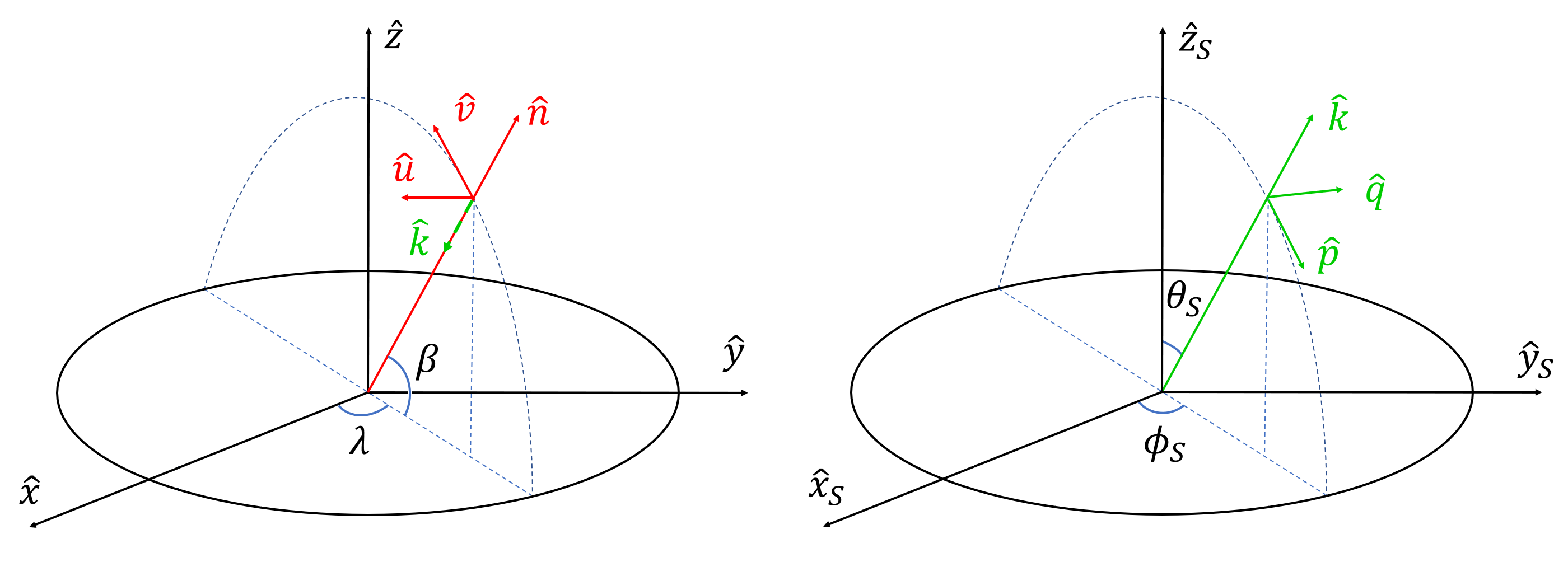
Figure 1: (Left) The detector frame and the relative orientation between $(\hat{x},\hat{y},\hat{z})$ and $(\hat{n},\hat{u},\hat{v})$. (Right) The source frame and the relative orientation between $(\hat{x}_{S},\hat{y}_{S},\hat{z}_{S})$ and $({\hat{k}},\hat{p},\hat{q})$.

The source frame is illustrated in Fig. 1 (Right). Exactly how the origin and the axes, $(\hat{x}_{S},\hat{y}_{S},\hat{z}_{S})$, are chosen for the source dynamics will be determined on a case-by-case basis. The direction to the GW detector is indicated with the unit vector ${\hat{k}}={\hat{k}}(\theta_{S},\phi_{S})\,$. To describe the polarization of GWs propagating along ${\hat{k}}\,$, two auxiliary unit vectors are also introduced,

$$\hat{q}=\frac{\hat{z}\times{\hat{k}}}{|\hat{z}\times{\hat{k}}|}\,,\quad\hat{p}=\hat{q}\times{\hat{k}}\,,$$ (5)

so that the trio, $(\hat{p},\hat{q},{\hat{k}})\,$, forms a right-handed orthogonal basis. Then, one can obtain that

$${\hat{p}}= \left[\cos\iota\cos\varphi,\ \sin\varphi\cos\iota,\ -\sin\iota\right],$$ (6)

$${\hat{q}}= \left[-\sin\varphi,\ \cos\varphi,\ 0\right],$$ (7)

$${\hat{k}}= \left[\sin\iota\cos\varphi,\ \sin\iota\sin\varphi,\ \cos\iota\right].$$ (8)

Since ${\hat{n}}=-{\hat{k}}\,$, the planes spanned by $(\hat{u},\hat{v})$ and $(\hat{p},\hat{q})$ are parallel to each other (see Fig. 2). As a result,

$$\hat{p}= \cos\psi\,\hat{u}+\sin\psi\,\hat{v}\,,\quad\hat{q}=-\sin\psi\,\hat{u}+\cos\psi\,\hat{v}\,,$$

$$\hat{u}= \cos\psi\,\hat{p}-\sin\psi\,\hat{q}\,,\quad\hat{v}=\sin\psi\,\hat{p}+\cos\psi\,\hat{q}\,.$$ (9)

Thus, the polarization angle can be computed as

$$\psi=\mathrm{arctan}_{2}\left[{\hat{p}}\cdot{\hat{u}},{\hat{p}}\cdot{\hat{v}}\right].$$ (10)

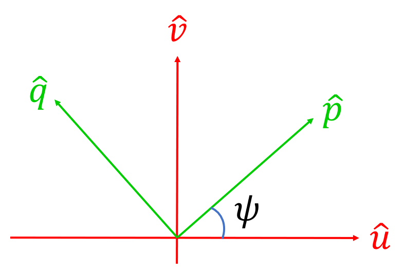
Figure 2: Relative orientations of $(\hat{u},\hat{v})$ and $(\hat{p},\hat{q})\,$. Note that ${\hat{k}}$ is perpendicular to and coming out of the paper.

Using the basis vectors, one can define the polarization tensors in the source frame and SSB frame. In the source frame

$$e^{+}_{ij}=({\hat{p}}\otimes{\hat{p}}-{\hat{q}}\otimes{\hat{q}})_{ij},\quad e^{\times}_{ij}=({\hat{p}}\otimes{\hat{q}}+{\hat{q}}\otimes{\hat{p}})_{ij}.$$ (11)

Similarly, in the SSB frame

$$\epsilon^{+}_{ij}=({\hat{u}}\otimes{\hat{u}}-{\hat{v}}\otimes{\hat{v}})_{ij},\quad\epsilon^{\times}_{ij}=({\hat{u}}\otimes{\hat{v}}+{\hat{v}}\otimes{\hat{u}})_{ij}.$$ (12)

After some calculation, the relation between the polarization tensors can be rewritten as

$$e^{+}= \epsilon^{+}\cos 2\psi+\epsilon^{\times}\sin 2\psi,$$ (13)

$$\quad e^{\times}= -\epsilon^{+}\sin 2\psi+\epsilon^{\times}\cos 2\psi.$$ (14)

In the source frame, the GW strain in a transverse-traceless gauge takes the form

$$h_{ij}^{TT}=e^{+}_{ij}h_{+}+e^{\times}_{ij}h_{\times},$$ (15)

where $h_{+,\times}$ are the plus and cross mode of GW. The corresponding representation of the strain in the SSB frame is

$$h_{ij}^{TT}=h_{+}(\epsilon^{+}\cos 2\psi+\epsilon^{\times}\sin 2\psi)_{ij}+h_{\times}(\epsilon^{\times}\cos 2\psi-\epsilon^{+}\sin 2\psi)_{ij}.$$ (16)

III Detectors

The three SBDs, TianQin, LISA, and TaiJi, all consist of three identical spacecraft that form a nearly equilateral triangle. The main difference is in their orbits: TianQin is placed on nearly identical nearly circular geocentric orbits with a radius of about $10^{5}$ km Luo et al. (2016). The detector plane of TianQin is directed towards the calibration source RX J0806.3+1527. In contrast, LISA and TaiJi are placed on Earth-like heliocentric orbits with a semi-major axis of about 1 astronomical unit (AU) from the Sun Amaro-Seoane et al. (2017); Hu and Wu (2017), and their detector plane rotates around in a yearly cycle. The arm length of TianQin is about $1.7\times 10^{5}$ km, while those of LISA and TaiJi are about $2.5\times 10^{6}$ km and $3\times 10^{6}$ km, respectively. The centre of LISA is approximately $20$ degrees behind the Earth, while that of TaiJi is approximately $20$ degrees ahead of the Earth Gong et al. (2021) (see Fig. 3). By selecting a geocentric orbit, TianQin is able to transmit data back to Earth in nearly real-time, making it more adapted to multi-messenger astronomy Chen et al. (2023).

In the following subsections, we utilize the Keplerian orbit to approximate the motion of the spacecraft in the SSB.

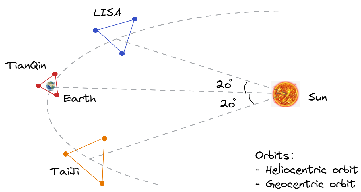
Figure 3: Schematic of the spacecraft’s orbit in the SSB coordinate system.

III.1 TianQin: geocentric orbit

In Fig. 4, we present a schematic of the spacecraft orbits for TianQin. The $x$-axis is defined as the direction from the Sun to the September equinox, while the $z$-axis represents the angular momentum direction of the Earth. For detailed information on the derivatives for the Keplerian orbit of TianQin, please refer to Ref. Hu et al. (2018).

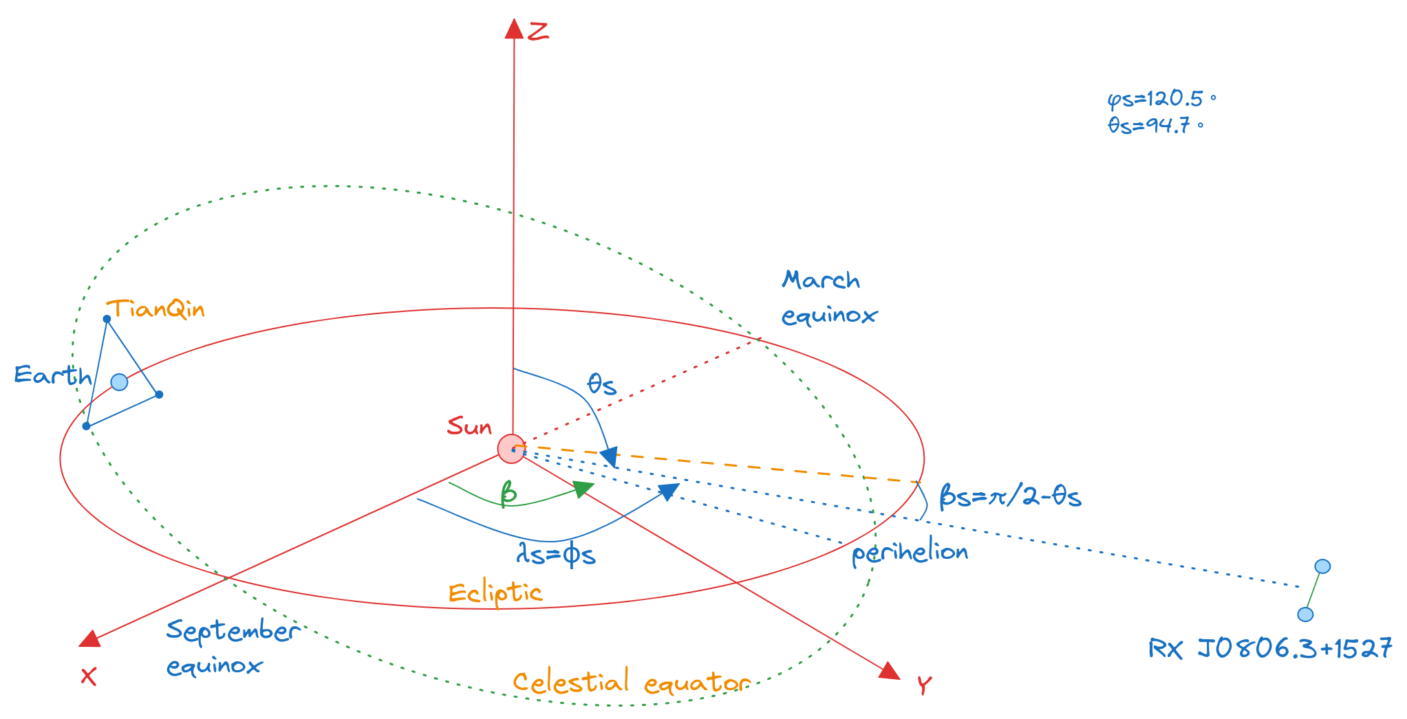
Figure 4: Schematic of the TianQin spacecraft’s orbit for TianQin in the SSB coordinate system.

The following presents a simplified and non-realistic depiction of the orbit, focusing on the motion of the Earth’s centre or guiding centre in the SSB frame:

$$X(t)= R\left[\cos(\alpha-\beta)-e(1+\sin^{2}(\alpha-\beta))-\frac{3}{2}e^{2}\cos(\alpha-\beta)\sin^{2}(\alpha-\beta)\right],$$ (17)

$$Y(t)= R\left[\sin(\alpha-\beta)+e\sin(\alpha-\beta)\cos(\alpha-\beta)+\frac{1}{2}e^{2}\sin(\alpha-\beta)(1-3\sin^{2}(\alpha-\beta))\right],$$ (18)

$$Z(t)= 0,$$ (19)

where $\alpha=2\pi f_{m}t+\kappa_{0}$, $f_{m}=1/(\text{one sidereal year})=3.14\times 10^{-8}$ Hz is the orbit modulation frequency, $\kappa_{0}$ is the mean ecliptic longitude measured from the vernal equinox (or September equinox) at $t=0$, and $\beta$ denotes the angle measured from the vernal equinox to the perihelion.

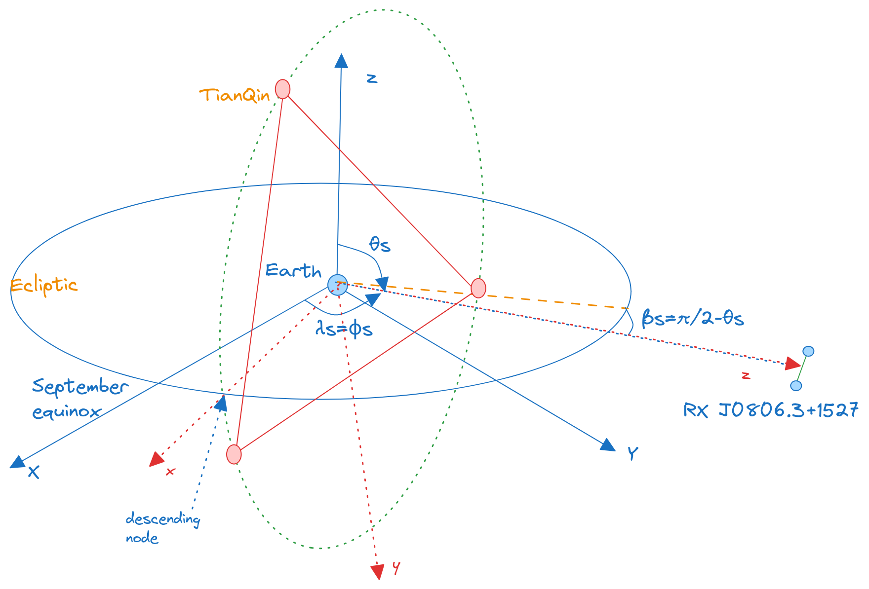
Figure 5: Schematic of the detector coordinate system $\{\tilde{x},\tilde{y},\tilde{z}\}$ and the geocentric-ecliptic coordinate system $\{x,y,z\}$. $\tilde{x}$ point to the descending node, $\tilde{z}$ axis points to J0806.

In the context of the TianQin spacecraft’s motion around the Earth, its orbits remain consistent with Eq. (19). However, when considering the SSB frame, TianQin assumes a specific orientation towards the direction of J0806 ($\{\lambda_{s},\beta_{s}\}=\{120.5^{\circ},-4.7^{\circ}\}$, as shown in Fig. 5). Introducing a coordinate system rotation and disregarding eccentricity, the description of TianQin’s orbits can be further refined Hu et al. (2018)

$$x_{n}= \frac{L}{\sqrt{3}}\left[\sin\beta_{s}\cos\lambda_{s}\sin(\alpha_{n}-\beta^{\prime})+\sin\lambda_{s}\cos(\alpha_{n}-\beta^{\prime})\right],$$ (20)

$$y_{n}= \frac{L}{\sqrt{3}}\left[\sin\beta_{s}\sin\lambda_{s}\sin(\alpha_{n}-\beta^{\prime})-\cos\lambda_{s}\cos(\alpha_{n}-\beta^{\prime})\right],$$ (21)

$$z_{n}= -\frac{L}{\sqrt{3}}\cos\beta_{s}\sin(\alpha_{n}-\beta^{\prime}),$$ (22)

where $L=\sqrt{3}\,R_{tq}$ is the arm-length between the two spacecraft, $\alpha(t)=2\pi f_{sc}t+\kappa_{n}$, $\kappa_{n}=+\frac{2}{3}\pi(n-1)+\lambda$, $\lambda$ is the initial orbit phase of the first ($n=1$) spacecraft measured from $\tilde{x}$ axis, $f_{sc}=1/\sqrt{GM_{Earth}/R_{tq}^{3}}\simeq 1/(3.65\,\rm day)$ is the modulation frequency due to the rotation of the detector around the guiding centre, $\beta^{\prime}$ is the angle measured from the $\tilde{x}$ axis to the perigee of the first spacecraft orbit. Here, we assume the three spacecraft are in circular orbits around the Earth, thus $\beta^{\prime}$ will be some arbitrary number (one can just set it as $0$).

III.2 LISA and TaiJi: heliocentric orbit

According to the description in Ref. Rubbo et al. (2004), when considering a constellation of spacecraft in individual Keplerian orbits with an inclination of $\iota=\sqrt{e}$, the coordinates of each spacecraft can be elegantly expressed in the following form (this expression has been expanded up to the second order of eccentricity) Rubbo et al. (2004)

$$x_{n}= a\cos(\alpha^{\prime\prime})+ae\left(\sin\alpha^{\prime\prime}\cos\alpha^{\prime\prime}\sin\beta_{n}^{\prime}-(1+\sin^{2}\alpha^{\prime\prime})\cos\beta_{n}^{\prime}\right)$$

$$+\frac{1}{8}ae^{2}\left(3\cos(3\alpha^{\prime\prime}-2\beta_{n}^{\prime})-10\cos\beta_{n}^{\prime}-5\cos(\alpha^{\prime\prime}-2\beta_{n}^{\prime})\right),$$ (23)

$$y_{n}= a\sin(\alpha^{\prime\prime})+ae\left(\sin\alpha^{\prime\prime}\cos\alpha^{\prime\prime}\cos\beta_{n}^{\prime}-(1+\cos^{2}\alpha^{\prime\prime})\sin\beta_{n}^{\prime}\right)$$

$$+\frac{1}{8}ae^{2}\left(3\sin(3\alpha^{\prime\prime}-2\beta_{n}^{\prime})-10\sin\alpha^{\prime\prime}+5\sin(\alpha^{\prime\prime}-2\beta_{n}^{\prime})\right),$$ (24)

$$z_{n}= -\sqrt{3}ae\cos(\alpha^{\prime\prime}-\beta_{n}^{\prime})+\sqrt{3}ae^{2}\left[1+\sin^{2}(\alpha^{\prime\prime}-\beta_{n}^{\prime})\right].$$ (25)

Here $a=R_{LISA,TJ}=1$ AU is the radial distance to the guiding center for LISA and TaiJi, $\alpha^{\prime\prime}=\alpha-\beta\mp 20^{\circ}$ for LISA and TaiJi, where $\alpha$ and $\beta$ is same as that in Earth orbit or in Eqs. (17)-(19). And $\beta_{n}^{\prime}=\frac{2\pi}{3}(n-1)+\lambda^{\prime}$, $\lambda^{\prime}$ is the initial orientation of the constellation, $e\simeq L_{LISA,TJ}/(2a\sqrt{3})$ represent the orbital eccentricity, $L_{LISA}=2.5\times 10^{6}$ km and $L_{TJ}=3\times 10^{6}$ km is the arm-length between two spacecraft for LISA and TaiJi, respectively.

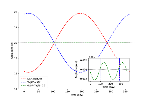
Figure 6: The relative angle between different detectors. Here, for improved visual clarity, the angle between LISA and TaiJi has been adjusted by subtracting 20 degrees.

While the spacecraft orbits for LISA and TaiJi are situated in the ecliptic planes, their constellation’s guiding centre follows a nearly circular trajectory. In the GWSpace code, the perihelion angle of the three spacecraft for LISA and TaiJi is set to be the same as that of Earth. However, TianQin’s guiding centre coincides with Earth’s, resulting in the changing angle between LISA and TaiJi over time. Figure 6 illustrates the relative angles between the different detectors. It can be observed that the angle between LISA or TaiJi and Earth varies between $18^{\circ}$ and $22^{\circ}$, while the angle between LISA and TaiJi is approximately $40^{\circ}$, with a slight variation of around $2.4\times 10^{-3}$. These findings are consistent with the proposed orbit described in Ref. Amaro-Seoane et al. (2017); Hu and Wu (2017).

IV Detector response

In a vacuum, propagating GWs induce a time-varying strain in the fabric of space-time. This strain can alter the proper distance between freely falling masses, providing a means to gather information about the GWs. One approach is to measure the variation in light travel time or optical path length between two test masses Jolien D. E. Creighton (2011). As a GW passes through, these separated masses will experience relative acceleration or tilting. Consequently, a GW detector is employed to monitor the separation between the test masses. There are two commonly used methods to monitor the distance between two objects: radar ranging or similar techniques, and measuring the Doppler shift in a signal transmitted from one object to the other Jolien D. E. Creighton (2011). However, a question arises regarding whether the GW affects the electromagnetic waves used for measuring distances Jolien D. E. Creighton (2011). In the following sections, we will provide a brief overview of how a GW detector responds to GW signals.

IV.1 The general waveform and mode decomposition

Assuming a universe consisting solely of vacuum and GW. Since GWs are very weak, the metric of the spacetime perturbated by a GW can be described as

$$ds^{2}=-c^{2}dt^{2}+\left[\delta_{ij}+h_{ij}(t)\right]dx^{i}dx^{j},$$ (26)

where $h_{ij}$ is the tensor perturbation, it is directly related to the GW itself, carrying information about its amplitude, frequency, and polarization. By analyzing the changes in the metric caused by the GW, we can extract valuable information about the GW signal. In the TT coordinate system (with coordinates $x^{0}=ct,x^{1}=x,x^{2}=y,x^{3}=z$), a weak GW can be described as a weak plane wave travelling in the $+z$ direction. The line element describes the metric of spacetime in this scenario is given by

$$ds^{2}=-c^{2}dt^{2}+\left(1+h_{+}\left(t-\frac{z}{c}\right)\right)dx^{2}+\left(1-h_{+}\left(t-\frac{z}{c}\right)\right)dy^{2}+2h_{\times}\left(t-\frac{z}{c}\right)dxdy+dz^{2}.$$ (27)

General waveform

The GW can be approximated as an arbitrary plane wave with wave vector $\vec{k}$ and a tensorial ‘amplitude’, thus

$${\bf h}(t,{\bf r})={\bf h}_{0}e^{\mathrm{i}(2\pi ft-\vec{k}\cdot{\bf r}/c)}={\bf h}_{0}e^{\mathrm{i}2\pi f(t-{\hat{k}}\cdot{\bf r}/c)}=h(t-{\hat{k}}\cdot{\bf r})=h(\xi),$$ (28)

where ${\hat{k}}=\frac{\vec{k}}{|\vec{k}|}=\frac{\vec{k}}{2\pi f}$ is the propagation direction of GW, ${\bf r}$ is an arbitrary direction, $\xi=t-{\hat{k}}\cdot{\bf r}$ is a surface of constant phase.

There is relative motion between the source frame and the detector frame. In the detector frame, the SSB is moving relative to the cosmic microwave background (CMB) with a peculiar velocity $v\approx 370$ km/s $\approx 0.0012$, along the direction $\lambda\approx 172^{\circ}\,$, $\beta\approx-11^{\circ}$ Kogut et al. (1993). In the source frame, the velocities of the sources can be introduced as model parameters.

Mode decomposition

In the source frame, the gravitational wave can be further decomposed using spin-weighted spherical harmonics Goldberg et al. (1967) ${}_{-2}Y_{\ell m}(\iota,\varphi)$ as

$$h_{+}-\mathrm{i}h_{\times}=\sum_{\ell\geq 2}\sum_{m=-\ell}^{\ell}{}_{-2}Y_{\ell m}(\iota,\varphi)h_{\ell m}.$$ (29)

where $\{\iota,\varphi\}$ represent the inclination and phase describing the orientation of emission. The primary harmonic is $h_{22}$, while the others are called higher harmonics or higher modes. And each mode can be described as

$$h_{\ell m}=A_{\ell m}e^{-\mathrm{i}\Phi_{\ell m}}.$$ (30)

Based on this decomposition, we obtain

$$h_{+}= \frac{1}{2}\sum_{\ell,m}\left({}_{-2}Y_{\ell m}(\iota,\varphi)h_{\ell m}+{}_{-2}Y_{\ell m}^{*}(\iota,\varphi)h_{\ell m}^{*}\right),$$ (31)

$$h_{\times}= \frac{\mathrm{i}}{2}\sum_{\ell,m}\left({}_{-2}Y_{\ell m}(\iota,\varphi)h_{\ell m}-{}_{-2}Y_{\ell m}^{*}(\iota,\varphi)h_{\ell m}^{*}\right).$$ (32)

In particular, for the non-processing binary systems with a fixed equatorial plane of orbit, there exists an exact symmetry relation between modes

$$h_{\ell,-m}=(-1)^{\ell}h^{*}_{\ell m}.$$ (33)

With this symmetry, one has

$$h_{+,\times}=\sum_{\ell,m}K_{\ell m}^{+,\times}h_{\ell m},$$ (34)

where

$$K_{\ell m}^{+}=\frac{1}{2}\left({}_{-2}Y_{\ell m}+(-1)^{\ell}{}_{-2}Y_{\ell,-m}^{*}\right),\qquad K_{\ell m}^{\times}= \frac{\mathrm{i}}{2}\left({}_{-2}Y_{\ell m}-(-1)^{\ell}{}_{-2}Y_{\ell,-m}^{*}\right).$$ (35)

It is convenient to introduce mode-by-mode polarization matrices

$$P_{\ell m}=e_{+}K_{\ell m}^{+}+e_{\times}K_{\ell m}^{\times},$$ (36)

so that the GW signal in matrix form will be

$${\bf h}^{TT}=\sum_{\ell,m}P_{\ell m}h_{\ell m}.$$ (37)

In the SSB frame, one can write

$$P_{+}+\mathrm{i}P_{\times}=e^{-\mathrm{i}2\psi}(\epsilon_{+}+\mathrm{i}\epsilon_{\times}).$$ (38)

With the above equations, $P_{\ell m}$ will be

$$P_{\ell m}(\iota,\varphi,\psi)=\frac{1}{2}{}_{-2}Y_{\ell m}(\iota,\varphi)e^{-\mathrm{i}2\psi}(\epsilon_{+}+\mathrm{i}\epsilon_{\times})+\frac{1}{2}(-1)^{\ell}{}_{-2}Y_{\ell,-m}^{*}(\ell,\varphi)e^{+\mathrm{i}2\psi}(\epsilon_{+}-\mathrm{i}\epsilon_{\times}).$$ (39)

In this way, we can factor out explicitly all dependencies in the extrinsic parameters $(\iota,\varphi,\psi)$.

Suppose that the GW only has the main mode, i.e., the 22 mode, we have $h_{22}=A_{22}e^{-\mathrm{i}\Phi_{22}}$ and $h_{2,-2}=h_{22}^{*}=A_{22}e^{\mathrm{i}\Phi}$. The expressions of the spin-weighted spherical harmonics for the mode of $\{2,\pm 2\}$ are

$${}_{-2}Y_{22}(\iota,\varphi)=\frac{1}{2}\sqrt{\frac{5}{\pi}}\cos^{4}\frac{\iota}{2}e^{\mathrm{i}2\varphi},\qquad{}_{-2}Y_{2,-2}(\iota,\varphi)=\frac{1}{2}\sqrt{\frac{5}{\pi}}\sin^{4}\frac{\iota}{2}e^{-\mathrm{i}2\varphi},$$ (40)

and

$$K_{22}^{+}= \frac{1}{2}\big{(}{}_{-2}Y_{22}(\iota,\varphi)+{}_{-2}Y_{2,-2}^{*}(\iota,\varphi)\big{)}=\frac{1}{4}\sqrt{\frac{5}{\pi}}\left(\cos^{4}\frac{\iota}{2}+\sin^{4}\frac{\iota}{2}\right)e^{\mathrm{i}2\varphi}=\frac{1}{4}\sqrt{\frac{5}{\pi}}\frac{\left(1+\cos^{2}\iota\right)}{2}e^{\mathrm{i}2\varphi},$$ (41)

$$K_{22}^{\times}= \frac{\mathrm{i}}{2}\big{(}{}_{-2}Y_{22}(\iota,\varphi)-{}_{-2}Y_{2,-2}^{*}(\iota,\varphi)\big{)}=\frac{\mathrm{i}}{4}\sqrt{\frac{5}{\pi}}\left(\cos^{4}\frac{\iota}{2}-\sin^{4}\frac{\iota}{2}\right)e^{\mathrm{i}2\varphi}=-\frac{\mathrm{i}}{4}\sqrt{\frac{5}{\pi}}\cos\iota e^{\mathrm{i}2\varphi}.$$

and so

$$K_{2,-2}^{+}=(K_{22}^{+})^{*},\qquad K_{2,-2}^{\times}=(K_{22}^{\times})^{*}.$$ (42)

Thus, one has

$$h_{+}= K_{22}^{+}h_{22}+K_{2,-2}^{+}h_{2,-2}=A_{22}\sqrt{\frac{5}{4\pi}}\frac{1+\cos^{2}\iota}{2}\cos(\Phi_{22}-2\varphi),$$ (43)

$$h_{\times}= K_{22}^{\times}h_{22}+K_{2,-2}^{\times}h_{2,-2}=A_{22}\sqrt{\frac{5}{4\pi}}\cos\iota\sin(2\Phi_{22}-2\varphi).$$ (44)

For non-precessing systems, Eq. (33) will be translate to

$${\tilde{h}}_{\ell,-m}(f)=(-1)^{\ell}{\tilde{h}}_{\ell m}(-f)^{*}$$ (45)

in the Fourier domain. For a given mode of GW waveform, one has $h_{\ell m}\propto\exp[-\mathrm{i}m\phi_{orbit}]$, where $\phi_{orbit}$ is the orbital phase of the GW systems, and it always verifying with $\dot{\phi}_{orbit}>0$. Thus, for non-precessing systems or in the processing frame for a binary with misaligned spins, an approximation often applied as

$${\tilde{h}}_{\ell m}(f)\simeq 0\quad\text{ for }m>0,\quad f>0,$$ (46)

$${\tilde{h}}_{\ell m}(f)\simeq 0\quad\text{ for }m<0,\quad f<0,$$

$${\tilde{h}}_{\ell 0}(f)\simeq 0.$$

In this way, for the positive frequencies $f>0$, ${\tilde{h}}_{+,\times}=\sum_{\ell}\sum_{m<0}K^{+,\times}_{\ell,m}{\tilde{h}}_{\ell m}$.

Eccentric mode decomposition

Eccentric waveforms also generate the harmonics, which act similarly to higher modes but are described by the mean orbital frequency. Under the stationary phase approximation (SPA), there is a relationship between the mean orbital frequency $F$ and the Fourier frequency $f$ for different eccentric harmonics:

$$f=j\cdot F(t_{0}).$$ (47)

Here we use the index $j$ to distinguish eccentric harmonics from spin-weighted spherical harmonics above. $t_{0}$ is the time which gives the stationary point of $F$. The dominant eccentric harmonic is $j=2$.

With $(\ell,m)=(2,2)$, a frequency domain eccentric waveform can be written as

$$\tilde{h}_{+,\times}=\sum_{j=1}^{10}\tilde{\mathcal{A}}_{j}\xi_{j}^{+,\times}e^{-{\rm i}\Psi_{j}}.$$ (48)

Here

$$\xi_{j}^{+,\times}=C_{+,\times}^{(j)}+{\rm i}S_{+,\times}^{(j)},$$ (49)

which is a function of $(\iota,\varphi)$ and the eccentricity $e(F)$. When $e=0$,

$$\xi_{j=2}^{+} =C_{+}^{(2)}+{\rm i}S_{+}^{(2)}=4\cdot\frac{{1+{{\cos}^{2}}\iota}}{2}{e^{{\rm i}\cdot 2\varphi}},$$ (50)

$$\xi_{j=2}^{\times} =C_{\times}^{(2)}+{\rm i}S_{\times}^{(2)}=4\cdot\left({-\cos\iota}\right){e^{{\rm i}\cdot 2\varphi}},$$

$$\xi_{j\neq 2}^{+,\times} =0,$$

which go back to the coefficients of the dominant mode $(\ell,m)=(2,2)$Yunes et al. (2009). But for a non-zero eccentricity, one cannot explicitly write $P_{\ell m}$ as we shown in Eq. (39), and should directly use $P_{+},P_{\times}$ in Eq. (38).

IV.2 Single arm response in time domain

The effect of GWs on matter can be described as a tidal deformation. To detect the GW, one method is to test the distance changes between two spatially separated free-falling test masses. Suppose that the photon travels along the direction of test mass 1 ($S_{s}$) to test mass 2 ($S_{r}$) as ${\hat{n}}_{l}$, as shown in Fig. 7. It follows a null geodesic, i.e., $ds^{2}=0$. Thus, the metric reads

$$cdt=\sqrt{(\delta_{ij}+h_{ij}(\xi))dx^{i}dx^{j}},$$ (51)

where

$$\xi(l)=t(l)-{\hat{k}}\cdot{\bf r}(l)/c=t_{s}+l/c-{\hat{k}}\cdot\left[{\bf r}_{s}(t_{s})+{\hat{n}}(t_{s})\,l\right]/c,$$ (52)

${\bf r}_{s}$ is the position of $S_{s}$, ${\bf r}(l)$ is the position of photon at time $t$, $l=\sqrt{\sum_{i}(x^{i}-x_{s}^{i})^{2}}=|{\bf r}(l)-{\bf r}_{s}|$, ${\hat{n}}=\frac{{\bf r}(l)-{\bf r}_{s}}{l}$, and

$$\frac{d\xi}{dl/c}=1-{\hat{k}}\cdot{\hat{n}}_{l}(t_{s}),\quad\frac{dx^{i}}{dl}={\hat{n}}^{i},\quad{\hat{n}}^{i}{\hat{n}}_{i}=1\quad\Rightarrow\quad\frac{dx^{i}/c}{d\xi}=\frac{dx^{i}}{dl}\frac{dl/c}{d\xi}=\frac{{\hat{n}}^{i}}{1-{\hat{k}}\cdot{\hat{n}}}$$ (53)

With the above derivation, Eq. (51) can be rewritten as

$$dt= \sqrt{(\delta_{ij}+h_{ij}(\xi))\frac{dx^{i}/c}{d\xi}\frac{dx^{j}/c}{d\xi}}d\xi=\sqrt{1+h_{ij}{\hat{n}}^{i}{\hat{n}}^{j}}\frac{d\xi}{1-{\hat{k}}\cdot{\hat{n}}}$$ (54)

$$\approx \left(1+\frac{1}{2}h_{ij}{\hat{n}}^{i}{\hat{n}}^{j}+\mathcal{O}(h^{2})\right)\frac{d\xi}{1-{\hat{k}}\cdot{\hat{n}}}.$$

Figure 7: A radio signal send from the point $S_{s}$ travels along the arm $L_{l}$ in the direction of ${\hat{n}}_{l}$ towards the receiver at $S_{r}$. The coordinate origin is denoted by $O$, while point $S_{s}$ and point $S_{r}$ are located at ${\bf r}_{s}$ and $S_{r}$, respectively.

Then, from $S_{s}$ to $S_{r}$, the duration of the proper time will be

$$\int_{t_{s}}^{t_{r}}dt= \int_{0}^{L_{l}}\sqrt{1+h_{ij}{\hat{n}}^{i}{\hat{n}}^{j}}\frac{d\xi}{1-{\hat{k}}\cdot{\hat{n}}}\approx\int_{0}^{L_{l}}\left(1+\frac{1}{2}{\hat{n}}_{l}^{T}\cdot{\bf h}\cdot{\hat{n}}_{l}+\mathcal{O}(h^{2})\right)\frac{d\xi}{1-{\hat{k}}\cdot{\hat{n}}_{l}}$$ (55)

$$= \int_{0}^{L_{l}}dl/c+\int_{0}^{L_{l}}\frac{{\hat{n}}_{l}^{T}\cdot{\bf h}\cdot{\hat{n}}_{l}}{2(1-{\hat{k}}\cdot{\hat{n}}_{l})}d\xi,$$

where $L_{l}$ is the length between $S_{s}$ and $S_{r}$, ${\hat{n}}_{l}$ is the unit vector of the photon propagation.

Here, if one supposes that the position of $S_{s}$ and $S_{r}$ does not change or changes very little during the photon moving from $S_{s}$ to $S_{r}$, which means ${\hat{n}}_{l}(t_{s})\approx{\hat{n}}_{l}(t_{r})={\hat{n}}_{l}$. Then, for simplicity, the integral in Eq. (55) can be rewritten as

$$t_{r}=t_{s}+L_{l}/c+\frac{1}{2(1-{\hat{k}}\cdot{\hat{n}}_{l})}{\hat{n}}_{l}^{T}\cdot\left(\int_{\xi_{s}}^{\xi_{r}}{\bf h}(\xi)d\xi\right)\cdot{\hat{n}}_{l}.$$ (56)

From this equation, one can directly get the path length fluctuations due to the GW

$$\delta l_{sr}(t)=\frac{c}{2(1-{\hat{k}}\cdot{\hat{n}}_{l})}{\hat{n}}_{l}^{T}\cdot\left(\int_{\xi_{s}}^{\xi_{r}}{\bf h}(\xi)d\xi\right)\cdot{\hat{n}}_{l}.$$ (57)

Suppose the frequency of the photon is not changed during the photon travel from $S_{s}$ to $S_{r}$. Then the total phase change of the photon will be $\phi_{\rm tot}=2\pi\nu_{0}(t_{r}-t_{s})$. If there is no GW, the phase change will be $\phi_{\rm ori}=2\pi\nu_{0}L/c$. So, with the help of Eq. (56), the phase fluctuations measured under the GW will be

$$\Delta\phi(t)=\phi_{\rm tot}-\phi_{\rm ori}=2\pi\nu_{0}\delta l_{sr}(t)/c.$$ (58)

To get the time of reception changes with respect to the time of emission, one can differentiate the above equation with respect to $t_{s}$

$$\frac{dt_{r}}{dt_{s}}= 1+\frac{1}{2(1-{\hat{k}}\cdot{\hat{n}}_{l})}{\hat{n}}_{l}^{T}\cdot\left(\int_{\xi_{0}}^{\xi_{L}}\frac{d{\bf h}(\xi)}{d\xi}\frac{d\xi}{dt_{s}}d\xi\right)\cdot{\hat{n}}_{l}$$ (59)

$$= 1+\frac{1}{2(1-{\hat{k}}\cdot{\hat{n}}_{l})}{\hat{n}}_{l}^{T}\cdot\left[{\bf h}(\xi_{r})-{\bf h}(\xi_{s})\right]\cdot{\hat{n}}_{l}.$$

Here, we have used the assumption that the motion of $S_{s}$ and $S_{r}$ is much slower compared to the time of laser beam propagation, i.e., $d{\bf r}_{s}/dt_{s}\approx 0$ and $d{\hat{n}}_{l}/dt_{s}\approx 0$, so $d\xi/dt_{s}=1$.

The interferometers used to detect GWs do not emit single photons but continuous lasers with frequency $\nu(t)$. If the phase change of the photon at $S_{s}$ and $S_{r}$ are the same, we have $d\phi/(2\pi)=\nu_{s}dt_{s}=\nu_{r}dt_{r}$. Then one can get the dimensionless fractional frequency deviation $y^{GW}(t)$ as

$$y_{sr}^{GW}(t_{r})= \frac{\nu_{r}-\nu_{s}}{\nu_{s}}=\frac{\nu_{r}}{\nu_{s}}-1=\frac{d\phi/dt_{r}}{d\phi/dt_{s}}-1$$ (60)

$$= \frac{1}{1+\frac{1}{2(1-{\hat{k}}\cdot{\hat{n}}_{l})}{\hat{n}}_{l}^{T}\cdot\left[{\bf h}(\xi_{r})-{\bf h}(\xi_{s})\right]\cdot{\hat{n}}_{l}}-1$$

$$\approx \frac{1}{2(1-{\hat{k}}\cdot{\hat{n}}_{l})}{\hat{n}}_{l}^{T}\cdot\left[{\bf h}(\xi_{s})-{\bf h}(\xi_{r})\right]\cdot{\hat{n}}_{l}+\mathcal{O}(h^{2}).$$

Hence

$$\xi_{s}= t_{s}-{\hat{k}}\cdot{\bf r}_{s}(t_{s})/c\approx t_{r}-L_{l}/c-{\hat{k}}\cdot[{\bf r}_{s}(t_{r}-L_{l}/c)]/c$$

$$\approx t_{r}-L_{l}/c-{\hat{k}}\cdot[{\bf r}_{s}(t_{r})-\partial_{t}{\bf r}_{s}(t_{r})L_{l}/c]/c$$

$$\approx t_{r}-L_{l}/c-{\hat{k}}\cdot{\bf r}_{s}(t_{r})/c,$$ (61)

$$\xi_{r}= t_{r}-{\hat{k}}\cdot{\bf r}_{r}(t_{r})/c.$$ (62)

In the third line, we have assumed that $\partial_{t}{\bf r}_{s}\ll c$. Finally, one has the relative frequency deviation at the time of $t=t_{r}$ as Wahlquist (1987); Armstrong et al. (1999); Katz et al. (2022)

$$y_{slr}^{GW}(t)=\frac{1}{2(1-{\hat{k}}\cdot{\hat{n}}_{l})}\,{\hat{n}}_{l}^{T}\cdot\left[{\bf h}(t-L_{l}/c-{\hat{k}}\cdot{\bf r}_{s}/c)-{\bf h}(t-{\hat{k}}\cdot{\bf r}_{r}/c)\right]\cdot{\hat{n}}_{l}.$$ (63)

When the photon reflected from $S_{r}$ to $S_{s}$, we have

$$y_{rls}^{GW}(t)=\frac{1}{2(1+{\hat{k}}\cdot{\hat{n}}_{l})}\,{\hat{n}}_{l}^{T}\cdot\left[{\bf h}(t-L_{l}/c-{\hat{k}}\cdot{\bf r}_{r}/c)-{\bf h}(t-{\hat{k}}\cdot{\bf r}_{s}/c)\right]\cdot{\hat{n}}_{l}.$$ (64)

Considering that the GW is described in the SSB coordinate, thus, one can redefine some parameters as

$$y_{slr}^{\rm GW}(t)=\frac{1}{2(1-{\hat{k}}\cdot{\hat{n}}_{l})}\left[H(t-L/c-{\hat{k}}\cdot{\bf r}_{s}/c)-H(t-{\hat{k}}\cdot{\bf r}_{r}/c)\right],$$ (65)

where

$$H(t)=n_{l}^{i}h_{ij}(t)n_{l}^{j}= n_{l}^{i}(h_{+}\epsilon_{ij}^{+}+h_{\times}\epsilon_{ij}^{\times})n_{l}^{j}=n_{l}^{i}\left[h_{+}(u_{i}u_{j}-v_{i}v_{j})+h_{\times}(u_{i}v_{j}+v_{i}u_{j})\right]n_{l}^{j}$$ (66)

$$= h_{+}(n_{l}^{i}u_{i}u_{j}n_{l}^{j}-n_{l}^{i}v_{i}v_{j}n_{l}^{j})+h_{\times}(n_{l}^{i}u_{i}v_{j}n_{l}^{j}+n_{l}^{i}v_{i}u_{j}n_{l}^{j})$$

$$= h_{+}\left[({\hat{n}}_{l}\cdot\hat{u})^{2}-({\hat{n}}_{l}\cdot\hat{v})^{2}\right]+h_{\times}\cdot 2({\hat{n}}_{l}\cdot\hat{u})({\hat{n}}_{l}\cdot\hat{v})$$

$$= h_{+}\zeta_{l}^{+}+h_{\times}\zeta_{l}^{\times},$$

and

$$\zeta_{l}^{+}= {\hat{n}}_{l}\cdot\epsilon^{+}\cdot{\hat{n}}_{l}=({\hat{n}}_{l}\cdot\hat{u})^{2}-({\hat{n}}_{l}\cdot\hat{v})^{2},$$ (67)

$$\zeta_{l}^{\times}= {\hat{n}}_{l}\cdot\epsilon^{\times}\cdot{\hat{n}}_{l}=2({\hat{n}}_{l}\cdot\hat{u})({\hat{n}}_{l}\cdot\hat{v}).$$ (68)

For the two-way response, one can get Estabrook and Wahlquist (1975)

$$y_{sls}^{GW}(t)= \frac{\nu}{\nu_{0}}-1=\frac{\nu}{\nu^{\prime}}\frac{\nu^{\prime}}{\nu_{0}}-1=\big{[}y_{slr}^{GW}(t-L_{l}/c)+1\big{]}\big{[}y_{rls}^{GW}(t)+1\big{]}-1$$ (69)

$$\approx y_{slr}^{GW}(t-L/c)+y_{rls}^{GW}(t)+\mathcal{O}(h^{2})$$

$$= \frac{1}{2}\bigg{\{}(1+{\hat{k}}\cdot{\hat{n}})\big{[}\Psi_{l}(t-2L_{l}/c)-\Psi_{l}(t-L/c)\big{]}+(1-{\hat{k}}\cdot{\hat{n}})\big{[}\Psi_{l}(t-L_{l}/c)-\Psi_{l}(t)\bigg{\}}$$

$$= \frac{1+{\hat{k}}\cdot{\hat{n}}}{2}\Psi_{l}(t-2L_{l}/c)-{\hat{k}}\cdot{\hat{n}}\,\Psi_{l}(t-L_{l}/c)-\frac{1-{\hat{k}}\cdot{\hat{n}}}{2}\Psi_{l}(t),$$

where (using ${\hat{n}}={\hat{n}}(t)$ for convenient)

$$\Psi_{l}(t^{\prime})=\frac{{\hat{n}}_{l}^{T}\cdot{\bf h}(t^{\prime}-{\hat{k}}\cdot{\bf r}(t^{\prime})/c)\cdot{\hat{n}}_{l}}{1-({\hat{k}}\cdot{\hat{n}}_{l})^{2}}.$$ (70)

However, one should note that the above derivation is based on the assumption that the positions of the spacecraft change very little between the photon send from $S_{s}$ to $S_{r}$.

IV.3 Single arm response in frequency domain

Adopting the Fourier transform, the GW in the frequency domain will be Romano and Cornish (2017)

$$h_{0}(t,\vec{x})=h(t-d(t))=\int dfe^{\mathrm{i}2\pi f(t-d(t))}\tilde{h}(f)\text{ or }h(\xi)=\int dfe^{\mathrm{i}2\pi f\xi}{\tilde{h}}(f).$$ (71)

With the Fourier transform, the path length fluctuations could be rewritten as

$$\delta l_{sr}(t)= \frac{c}{2(1-{\hat{k}}\cdot{\hat{n}}_{l})}{\hat{n}}_{l}^{T}\cdot\left(\int_{\xi_{s}}^{\xi_{r}}d\xi\int df\,e^{\mathrm{i}2\pi f\xi}\,\tilde{\mathbf{h}}(f)\right)\cdot{\hat{n}}_{l}$$ (72)

$$= \frac{c}{2(1-{\hat{k}}\cdot{\hat{n}}_{l})}{\hat{n}}_{l}^{T}\cdot\left(\int df\,\left(e^{\mathrm{i}2\pi f\xi_{r}}-e^{\mathrm{i}2\pi f\xi_{s}}\right)\frac{\tilde{\mathbf{h}}(f)}{\mathrm{i}2\pi f}\right)\cdot{\hat{n}}_{l}$$

$$= \,L_{l}\,{\hat{n}}_{l}^{T}\cdot\left(\int df\,e^{\mathrm{i}2\pi ft}\mathcal{T}_{sr}({\hat{k}},f,t)\tilde{\mathbf{h}}(f)\right)\cdot{\hat{n}}_{l}$$

where $\mathcal{T}_{sr}({\hat{k}},f,t)$ is the transfer function Romano and Cornish (2017)

$$\mathcal{T}_{sr}(f,t)= \frac{c/L}{2(1-{\hat{k}}\cdot{\hat{n}}_{l})}\,\frac{1}{\mathrm{i}2\pi f}\left(e^{-\mathrm{i}2\pi f{\hat{k}}\cdot{\bf r}_{r}/c}-e^{-\mathrm{i}2\pi f(L_{l}+{\hat{k}}\cdot{\bf r}_{s})/c}\right)$$ (73)

$$= \frac{c/L}{2(1-{\hat{k}}\cdot{\hat{n}}_{l})}\,\frac{1}{\mathrm{i}2\pi f}\left(e^{\mathrm{i}\pi f[L-{\hat{k}}\cdot({\bf r}_{r}-{\bf r}_{s})]/c}-e^{-\mathrm{i}\pi f[L_{l}-{\hat{k}}\cdot({\bf r}_{r}-{\bf r}_{s})]/c}\right)e^{-\mathrm{i}\pi f[L+{\hat{k}}\cdot({\bf r}_{r}+{\bf r}_{s})]/c}$$

$$= \frac{c/L}{2(1-{\hat{k}}\cdot{\hat{n}})}\,\frac{\mathrm{i}2\sin\left(\pi fL/c(1-{\hat{k}}\cdot{\hat{n}})\right)}{\mathrm{i}2\pi f}e^{-\mathrm{i}\pi f[L+{\hat{k}}\cdot({\bf r}_{r}+{\bf r}_{s})]/c}$$

$$= \frac{1}{2}{\rm sinc}\left(\pi fL/c(1-{\hat{k}}\cdot{\hat{n}})\right)\exp\left\{-\mathrm{i}\pi f[L+{\hat{k}}\cdot({\bf r}_{r}+{\bf r}_{s})]/c\right\}.$$

Finally, one can define the one-arm detector tensor as

$${\bf D}({\hat{k}},f,t)=\frac{1}{2}{\hat{n}}(t)\otimes{\hat{n}}(t)\,\mathcal{T}({\hat{k}},f,t),$$ (74)

and the path length fluctuation in the frequency domain will be

$$\frac{\delta{\tilde{l}}_{sr}(f)}{L_{l}}={\bf D}({\hat{k}},f,t)\,\mathbf{:}\,\tilde{\mathbf{h}}(f),$$ (75)

where $({\hat{n}}\otimes{\hat{n}})_{ij}={\hat{n}}_{i}{\hat{n}}_{j}$, ${\bf A}\mathbf{:}{\bf B}=A_{i}B_{i}$. Similarly, the phase fluctuation in the frequency domain will be

$$\Delta\tilde{\phi}(f)=\frac{2\pi\nu_{0}}{c}\delta{\tilde{l}}_{sr}(f).$$ (76)

On the other hand, we can derive the relative frequency derivation in the frequency domain directly through the Fourier transform. Fourier transforms the relative frequency deviation will be

$${\tilde{y}}_{slr}^{GW}(f,t)= \int dt\,e^{-\mathrm{i}2\pi ft}y_{slr}^{GW}(t)$$ (77)

$$= \frac{1}{2(1-{\hat{k}}\cdot{\hat{n}}_{l})}\,{\hat{n}}_{l}^{T}\cdot\left[\int dte^{-\mathrm{i}2\pi ft}\left[{\bf h}(t-L_{l}/c-{\hat{k}}\cdot{\bf r}_{s}/c)-{\bf h}(t-{\hat{k}}\cdot{\bf r}_{r}/c)\right]\right]\cdot{\hat{n}}_{l}$$

$$= \frac{1}{2(1-{\hat{k}}\cdot{\hat{n}}_{l})}\,{\hat{n}}_{l}^{T}\cdot\int dte^{-\mathrm{i}2\pi ft}\left[\int df^{\prime}e^{\mathrm{i}2\pi f^{\prime}(t-L_{l}/c-{\hat{k}}\cdot{\bf r}_{s}/c)}{\bf h}(f^{\prime})-\int df^{\prime\prime}e^{\mathrm{i}2\pi f^{\prime\prime}(t-{\hat{k}}\cdot{\bf r}_{r}/c)}{\bf h}(f^{\prime\prime})\right]\cdot{\hat{n}}_{l}$$

$$= \frac{1}{2(1-{\hat{k}}\cdot{\hat{n}}_{l})}\,{\hat{n}}_{l}^{T}\cdot\int dt\int df^{\prime}e^{-\mathrm{i}2\pi(f-f^{\prime})t}\tilde{\mathbf{h}}(f^{\prime})\left[e^{-\mathrm{i}2\pi f^{\prime}(L_{l}+{\hat{k}}\cdot{\bf r}_{s})/c}-e^{-\mathrm{i}2\pi f^{\prime}\,{\hat{k}}\cdot{\bf r}_{r}/c}\right]\cdot{\hat{n}}_{l}$$

$$= \frac{1}{2(1-{\hat{k}}\cdot{\hat{n}}_{l})}\,\left[e^{-\mathrm{i}2\pi f(L_{l}+{\hat{k}}\cdot{\bf r}_{s})/c}-e^{-\mathrm{i}2\pi f\,{\hat{k}}\cdot{\bf r}_{r}/c}\right]\,{\hat{n}}_{l}^{T}\cdot\tilde{\mathbf{h}}(f)\cdot{\hat{n}}_{l}$$

$$= \frac{1}{2(1-{\hat{k}}\cdot{\hat{n}}_{l})}\,\left[e^{-\mathrm{i}\pi f[L_{l}+{\hat{k}}\cdot({\bf r}_{s}-{\bf r}_{r})]/c}-e^{-\mathrm{i}\pi f({\hat{k}}\cdot{\bf r}_{r}-L_{l}-{\hat{k}}\cdot{\bf r}_{s})/c}\right]e^{-\mathrm{i}\pi f[L_{l}+{\hat{k}}\cdot({\bf r}_{s}+{\bf r}_{r})]/c}\,{\hat{n}}_{l}^{T}\cdot\tilde{\mathbf{h}}(f)\cdot{\hat{n}}_{l}$$

$$= -\frac{\mathrm{i}\sin\left[\pi fL_{l}/c(1-{\hat{k}}\cdot{\hat{n}}_{l})\right]}{(1-{\hat{k}}\cdot{\hat{n}}_{l})}\,e^{-\mathrm{i}\pi f[L_{l}+{\hat{k}}\cdot({\bf r}_{s}+{\bf r}_{r})]/c}\,{\hat{n}}_{l}^{T}\cdot\tilde{\mathbf{h}}(f)\cdot{\hat{n}}_{l}$$

$$= -\frac{\mathrm{i}\pi fL_{l}}{c}\mathrm{sinc}\left[\pi fL_{l}/c(1-{\hat{k}}\cdot{\hat{n}}_{l})\right]\,e^{-\mathrm{i}\pi f[L_{l}+{\hat{k}}\cdot({\bf r}_{s}+{\bf r}_{r})]/c}\,{\hat{n}}_{l}^{T}\cdot\tilde{\mathbf{h}}(f)\cdot{\hat{n}}_{l}$$

$$= -\frac{\mathrm{i}2\pi fL_{l}}{c}\mathcal{T}_{sr}(f,t)\,(h_{+}\zeta_{l}^{+}+h_{\times}\zeta_{l}^{\times}).$$

Here ${\hat{n}}_{l}\cdot\tilde{\mathbf{h}}(f)\cdot{\hat{n}}_{l}={\hat{n}}_{l}\cdot({\tilde{h}}_{+}\epsilon^{+}+{\tilde{h}}_{\times}\epsilon^{\times})\cdot{\hat{n}}_{l}={\tilde{h}}_{+}\zeta_{l}^{+}+{\tilde{h}}_{\times}\zeta_{l}^{\times}$. If the GW tensor can be decomposed into $\tilde{\mathbf{h}}=\mathbf{P}(f)\tilde{h}(f)$, where ${\bf P}=e^{+}+e^{\times}$. Thus, the transfer function for the relative frequency deviation can be written as Marsat and Baker (2018); Marsat et al. (2021)

$$G_{slr}^{GW}(f,t)=-\frac{\mathrm{i}\pi fL_{l}}{c}\mathrm{sinc}\left[\pi fL_{l}/c(1-{\hat{k}}\cdot{\hat{n}}_{l})\right]\,e^{-\mathrm{i}\pi f[L+{\hat{k}}\cdot({\bf r}_{s}+{\bf r}_{r})]/c}\,{\hat{n}}_{l}^{T}\cdot\mathbf{P}(f)\cdot{\hat{n}}_{l}.$$ (78)

For the multiple modes, the transfer function $G_{slr}^{\ell m}(f,t)$ has the same form as the above equation, where just ${\bf r}$ should be changed to $P_{\ell m}$, i.e.,

$$G_{slr}^{\ell m}(f,t)=-\frac{\mathrm{i}\pi fL_{l}}{c}\mathrm{sinc}\left[\pi fL_{l}/c(1-{\hat{k}}\cdot{\hat{n}}_{l})\right]\,e^{-\mathrm{i}\pi f[L+{\hat{k}}\cdot({\bf r}_{s}+{\bf r}_{r})]/c}\,{\hat{n}}_{l}^{T}\cdot P_{\ell m}\cdot{\hat{n}}_{l}.$$ (79)

With help of $\xi_{+}$ and $\xi_{\times}$, the part of ${\hat{n}}_{l}\cdot P_{\ell m}\cdot{\hat{n}}_{l}$ will be

$${\hat{n}}_{l}\cdot P_{\ell m}\cdot{\hat{n}}_{l}= \frac{1}{2}{}_{-2}Y_{\ell m}(\iota,\varphi)e^{-\mathrm{i}2\psi}(\zeta_{l}^{+}+\mathrm{i}\zeta_{l}^{\times})+\frac{1}{2}(-1)^{\ell}{}_{-2}Y_{\ell,-m}^{*}(\ell,\varphi)e^{+\mathrm{i}2\psi}(\xi_{l}^{+}-\mathrm{i}\xi_{l}^{\times}).$$ (80)

One should note that in the previous equations, when the higher modes are considered, the time-frequency relationship should be considered. With the help of stationary phase approximation, the time-frequency relationship will be

$$t_{f}^{\ell m}=-\frac{1}{2\pi}\frac{d\Psi_{\ell m}}{df},$$ (81)

for different modes.

As for GW with eccentricity, we could not simply calculate the response function using the formulae above, even if it only has the dominant spin-weighted spherical harmonic $(\ell,m)=(2,2)$. Different eccentric harmonics also have different time-frequency correspondence, so we need to write Wang et al. (2023)

$$t_{f}^{j}=\frac{1}{{2\pi}}\frac{{d{\Psi_{j}}}}{{df}}.$$ (82)

Then we decompose $\tilde{\mathbf{h}}$ into eccentric harmonics $\tilde{\mathbf{h}}_{j}$, i.e.

$$\tilde{\mathbf{h}} =\sum\limits_{j}\tilde{\mathbf{h}}_{j},$$ (83)

$${\tilde{\mathbf{h}}}_{j} ={{P_{+}}\tilde{h}_{j}^{+}+{P_{\times}}\tilde{h}_{j}^{\times}},$$

and rewrite Eq. (77)-(79):

$${{\tilde{y}}_{slr}}=\sum\limits_{j}{\mathcal{T}_{slr}^{j}(f):{\tilde{h}}_{j}},$$ (84)

$$\mathcal{T}_{slr}^{j}(f)={G_{slr}}\left({f,t_{f}^{j}}\right),$$ (85)

$$G_{slr}^{\ell m}(f,t)=-\frac{\mathrm{i}\pi fL_{l}}{c}\mathrm{sinc}\left[\pi fL_{l}/c(1-{\hat{k}}\cdot{\hat{n}}_{l})\right]\,e^{-\mathrm{i}\pi f[L+{\hat{k}}\cdot({\bf r}_{s}+{\bf r}_{r})]/c}\,{\hat{n}}_{l}^{T}\otimes{\hat{n}}_{l}.$$ (86)

IV.4 Response for the mildly chirping signals

For mildly chirping binary sources that do not contain the Fourier integral, one can assume that the phase of the GW can be approximated as Cornish and Rubbo (2003).

$$\Phi(\xi)=2\pi f_{0}\xi+\pi\dot{f}_{0}\xi^{2}+\varphi_{0},$$ (87)

where $f_{0},\dot{f}_{0}$ and $\varphi_{0}$ are the initial frequency, frequency deviation and phase, respectively. Thus, the instantaneous frequency can be given as

$$\frac{1}{2\pi}\frac{\partial\Phi(\xi)}{\partial t}=\frac{1}{2\pi}\frac{\partial\Phi(\xi)}{\partial\xi}\frac{\partial\xi}{\partial t}=(f_{0}+\dot{f}_{0}\xi)\left(1-{\hat{k}}\cdot\frac{\partial{\bf r}(t)}{\partial t}\right).$$ (88)

According to the equation, we may assume a fixed frequency at $\xi_{0}$ as

$$f_{s}=f_{0}+\dot{f}_{0}\xi_{0},$$ (89)

and the index $s$ denotes the dependency of the approximated frequency on the time of emission $\xi_{0}$. Here, assuming that the frequency of the GW changes very little, i.e., $\dot{f}_{0}(\xi_{L}-\xi_{0})\ll f_{0}$. Then

$$\Phi(\xi)\approx\int dt\,2\pi f_{s}\left(1-{\hat{k}}\cdot\frac{\partial{\bf r}(t)}{\partial t}\right)=\int d\xi\,2\pi f_{s}=2\pi(f_{0}+\dot{f}_{0}\xi_{0})\xi+C,$$ (90)

where $C$ is some integration constant. Meanwhile, the amplitude of the wave also changes little. Then the plane wave can be described as

$$h(\xi)=A(\xi)e^{\mathrm{i}2\pi f_{s}\xi}\approx A(\xi_{0})e^{\mathrm{i}2\pi f_{s}\xi_{0}}e^{\mathrm{i}2\pi f_{s}(\xi-\xi_{0})}=h(\xi_{0})e^{\mathrm{i}2\pi f_{s}(\xi-\xi_{0})}.$$ (91)

In this way, the integration of the GW tensor fluctuation will be Cornish and Rubbo (2003)

$$\int_{\xi_{0}}^{\xi_{L}}{\bf h}(\xi)d\xi= {\bf P}\int h(\xi_{0})e^{\mathrm{i}2\pi f_{s}(\xi-\xi_{0})}d\xi={\bf P}\frac{1}{\mathrm{i}2\pi f_{s}}\left(h(\xi_{L})-h(\xi_{0})\right)={\bf P}\frac{1}{\mathrm{i}2\pi f_{s}}h(\xi_{0})\left(e^{\mathrm{i}2\pi f_{s}(\xi_{L}-\xi_{0})}-1\right)$$ (92)

$$= {\bf P}\frac{\sin\left[\pi f_{s}(\xi_{L}-\xi_{0})\right]}{\pi f_{s}}e^{\mathrm{i}\pi f_{s}(\xi_{L}-\xi_{0})}h(\xi_{0})$$

$$= {\bf P}\frac{\sin\left[\pi f_{s}(\xi_{L}-\xi_{0})\right]}{\pi f_{s}}e^{\mathrm{i}\pi f_{s}(\xi_{L}+\xi_{0})}A(\xi_{0})$$

$$= {\bf P}\frac{(1-{\hat{k}}\cdot{\hat{n}})L}{c}{\rm sinc}\left[\frac{\pi f_{s}L}{c}\,(1-{\hat{k}}\cdot{\hat{n}})\right]e^{-\mathrm{i}\pi f_{s}[L+{\hat{k}}\cdot({\bf r}_{r}+{\bf r}_{s})]/c}A(\xi_{0})e^{\mathrm{i}2\pi f_{s}t_{r}}$$

$$= 2\,{\bf P}\frac{(1-{\hat{k}}\cdot{\hat{n}})L}{c}\mathcal{T}_{sr}({\hat{k}},f_{s},t_{r})A(\xi_{0})e^{\mathrm{i}2\pi f_{s}t_{r}},$$

where ${\bf P}$ is the unit tensor matrix of GW. Here we have used

$$\xi_{L}-\xi_{0}= (t_{r}-{\hat{k}}\cdot{\bf r}_{r})-(t_{s}-{\hat{k}}\cdot{\bf r}_{s})=(1-{\hat{k}}\cdot{\hat{n}})L/c,$$ (93)

$$\xi_{L}+\xi_{0}= (t_{r}-{\hat{k}}\cdot{\bf r}_{r}/c)+(t_{s}-{\hat{k}}\cdot{\bf r}_{s}/c)\approx 2t_{r}-L/c-{\hat{k}}\cdot({\bf r}_{s}+{\bf r}_{r})/c.$$

If the amplitude of GW is some constant, then the path length variation defined in Eq. (57) will be

$$\frac{\delta l_{sr}}{L}(t)\approx\mathcal{T}_{sr}({\hat{k}},f_{s},t)\,{\hat{n}}\cdot{\bf h}(t)\cdot{\hat{n}}.$$ (94)

And according to Eq. (60), one can find that

$$\frac{\delta\nu}{\nu_{0}}=-\frac{\mathrm{i}2\pi f_{s}L}{c}\frac{\delta l}{L}.$$ (95)

This is similar to the response in the frequency domain, and one should note that the above formula is valid only when the GW is some mildly chirping signals or some monochromatic signals.

V Time Delay Interference

The signal transmitted from spacecraft $s$ that is received at spacecraft $r$ at time $t_{r}$ has its phase compared to the local reference to give the output of the phase change $\Phi_{sr}(t_{r})$ Cornish and Rubbo (2003). The phase difference has contributions from the laser phase noise $C(t)$, optical path length variations, shot noise $n^{s}(t)$ and acceleration noise $\mathbf{n}^{a}(t)$ Cornish and Rubbo (2003)

$$\Phi_{slr}(t_{r})=\color[rgb]{1,0,0}\boxed{\color[rgb]{0,0,0}C_{s}(t_{s})-C_{r}(t_{r})}\color[rgb]{0,0,0}+2\pi\nu_{0}(\color[rgb]{0,1,1}\boxed{\color[rgb]{0,0,0}\delta l_{l}(t_{s})}\color[rgb]{0,0,0}+\color[rgb]{0,0,1}\boxed{\color[rgb]{0,0,0}\Delta l_{l}(t_{s})}\color[rgb]{0,0,0})+\color[rgb]{0,1,0}\boxed{\color[rgb]{0,0,0}n^{s}_{sr}(t_{r})}\color[rgb]{0,0,0}-{\hat{n}}_{l}(t_{s})\cdot\left[\color[rgb]{1,1,0}\boxed{\color[rgb]{0,0,0}\mathbf{n}^{a}_{sr}(t_{r})-\mathbf{n}^{a}_{rs}(t_{s})}\color[rgb]{0,0,0}\right],$$ (96)

where $t_{s}$ is given implicitly by $t_{s}=t_{r}-\ell_{sr}(t_{s})$ and $\nu_{0}$ is the laser frequency. The optical path length variations caused by gravitational waves is $\delta l_{l}(t_{s})$, and those caused by orbital effects is $\Delta l_{l}(t_{s})$. From Eq. (96), one can find that the space-based GW detection suffers from laser phase noise, which can be alleviated through TDI technology. TDI involves heterodyne interferometry with unequal arm lengths and independent phase-difference readouts Tinto and Dhurandhar (2021). By essentially constructing a virtually equal-arm interferometer, the laser phase noise cancels out exactly.

V.1 General TDI combination

Before introducing the TDI, let’s first introduce some definitions. In Fig. 8, the satellite numbers in space are defined clockwise. The definition of the laser path counterclockwise is the positive direction (${\hat{n}}_{i}$), denoted as $L_{i}$, and clockwise is the negative direction ($-{\hat{n}}_{i}$), denoted as $L^{\prime}_{i}$. The arm length $|L_{i}|$ is defined as the distance between the other two satellites facing the satellite $i$, where $i=1,2,3$.

Figure 8: Illustration of detector constellation. Three satellites are marked as 1, 2, and 3. Laser paths are marked as $L_{i}$ and $L^{\prime}_{i}$, where $L^{\prime}_{i}$ represents the direction opposite to $L_{i}$. The direction of unit vector ${\hat{n}}_{i}$ is the same as that of $L_{i}$.

As shown in Fig. 8, let $\vec{X}_{i}$ as the $i$-th spacecraft, $l_{ij}$ is the distance between the $i$-th and $j$-th spacecrafts, then

$$L_{1} =\vec{u}_{32}\,l_{32}=\vec{X}_{2}-\vec{X}_{3}\quad L_{2}=\vec{u}_{13}\,l_{13}=\vec{X}_{3}-\vec{X}_{1}\qquad L_{3}=\vec{u}_{21}\,l_{21}=\vec{X}_{1}-\vec{X}_{2}$$ (97)

$${\hat{n}}_{1} =\vec{u}_{32}=\frac{\vec{X}_{2}-\vec{X}_{3}}{|\vec{X}_{2}-\vec{X}_{3}|}\qquad{\hat{n}}_{2}=\vec{u}_{13}=\frac{\vec{X}_{3}-\vec{X}_{1}}{|\vec{X}_{3}-\vec{X}_{1}|}\qquad{\hat{n}}_{3}=\vec{u}_{21}=\frac{\vec{X}_{1}-\vec{X}_{2}}{|\vec{X}_{1}-\vec{X}_{2}|}$$ (98)

Let $s_{1}$ as the time-dependent phase change signals received by the $1$-th spacecraft, which is sent from the $2$-th spacecraft and propagates along the link $L_{3}$. One can also sign it as $s_{231}$. Similarly, let $s^{\prime}_{1}$ as the signal received by spacecraft $1$, which is sent from spacecraft $3$ and propagates along $L^{\prime}_{2}$, or recorded as $s_{321}$. As shown in Fig. 8 there are six independent laser links.

The first generation TDI combination does not consider the rotation and flexing of the spacecraft constellation, which is only valid for a static constellation, i.e.,

$$L_{i}(t)=L_{i}=\text{const},\qquad L_{i}=L_{i^{\prime}}.$$ (99)

This means that all the arm lengths remain constant as time evolves, and the time duration of photon propagation along the arm is independent of the direction of photons. The 1.5 or modified TDI generation is valid for a rigid but rotating spacecraft constellation, i.e.,

$$L_{i}(t)=L_{i}=\text{const},\qquad L_{i}\neq L_{i^{\prime}}.$$ (100)

The propagation direction of photons should be considered. The second generation TDI combination is applied to consider a rotating and flexing constellation, i.e.,

$$L_{i}(t)=L_{i}+\dot{L}_{i}\,t,\qquad L_{i}\neq L_{i^{\prime}}.$$ (101)

The arm length changes linearly in time, and relative to the velocity of $\dot{L}_{i}$. Here, define the time delay operator as $\mathcal{D}_{i}$, where

$$\mathcal{D}_{i}x(t) \equiv x(t-L_{i}/c),$$ (102)

$$\mathcal{D}_{i}\mathcal{D}_{j}x(t)=\mathcal{D}_{ij}\,x(t) \equiv x(t-L_{i}/c-L_{j}/c).$$ (103)

Then one can define the 1.5 generation unequal arm Michelson-like combination as (see Fig. 9) Armstrong et al. (1999)

$$X_{1.5}= y_{32^{\prime}1}+\mathcal{D}_{2^{\prime}}\left[y_{123}+\mathcal{D}_{2}\left(y_{231}+\mathcal{D}_{3}y_{13^{\prime}2}\right)\right]-y_{231}-\mathcal{D}_{3}\left[y_{13^{\prime}2}+\mathcal{D}_{3^{\prime}}\left(y_{32^{\prime}1}+\mathcal{D}_{2^{\prime}}y_{123}\right)\right]$$ (104)

$$= y_{32^{\prime}1}+\mathcal{D}_{2^{\prime}}y_{123}+\mathcal{D}_{2^{\prime}2}y_{231}+\mathcal{D}_{2^{\prime}23}y_{13^{\prime}2}-y_{231}-\mathcal{D}_{3}y_{13^{\prime}2}-\mathcal{D}_{33^{\prime}}y_{32^{\prime}1}-\mathcal{D}_{33^{\prime}2^{\prime}}y_{123}.$$

For the generation 2.0, one have Armstrong et al. (1999)

$$X_{2.0}= \,y_{32^{\prime}1}+\mathcal{D}_{2^{\prime}}y_{123}+\mathcal{D}_{2^{\prime}2}y_{231}+\mathcal{D}_{2^{\prime}23}y_{13^{\prime}2}$$ (105)

$$+\mathcal{D}_{2^{\prime}233^{\prime}}y_{231}+\mathcal{D}_{2^{\prime}233^{\prime}3}y_{13^{\prime}2}+\mathcal{D}_{2^{\prime}233^{\prime}33^{\prime}}y_{32^{\prime}1}+\mathcal{D}_{2^{\prime}233^{\prime}33^{\prime}2^{\prime}}y_{123}$$

$$-y_{231}-\mathcal{D}_{3}y_{13^{\prime}2}-\mathcal{D}_{33^{\prime}}y_{32^{\prime}1}-\mathcal{D}_{33^{\prime}2^{\prime}}y_{123}$$

$$-\mathcal{D}_{33^{\prime}2^{\prime}2}y_{32^{\prime}1}-\mathcal{D}_{33^{\prime}2^{\prime}22^{\prime}}y_{123}-\mathcal{D}_{33^{\prime}2^{\prime}22^{\prime}2}y_{231}-\mathcal{D}_{33^{\prime}2^{\prime}22^{\prime}23}y_{13^{\prime}2}.$$

The $Y$ and $Z$ channels can be generated by cyclic permutation of indices: $1\rightarrow 2\rightarrow 3\rightarrow 1$.

Figure 9: Michelson-like TDI-X channel of first generation TDI.

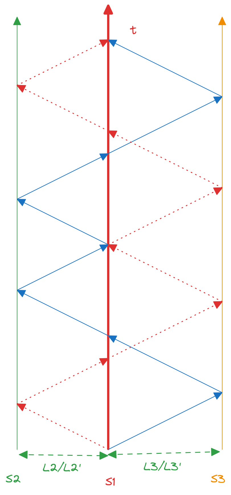
Figure 10: Space-time map of TDI 2.0 for the Michelson-like X channel.

Suppose that all the armlengths are equal, i.e., $L_{i}=L$. Thus, in the time domain, the first generation of TDI Michelson-like $X$ channel will be

$$X=[y_{32^{\prime}1}+\mathcal{D}y_{123}]+\mathcal{D}^{2}[y_{231}+\mathcal{D}y_{13^{\prime}2}]-[y_{231}+\mathcal{D}y_{13^{\prime}2}]-\mathcal{D}^{2}[y_{32^{\prime}1}+\mathcal{D}y_{123}],$$ (106)

where $\mathcal{D}=\mathcal{D}_{i}$ and $\mathcal{D}^{2}=\mathcal{D}\mathcal{D}$. Simply, let $y_{slr,nL}=y_{sr}(t-nL)$, its Fourier transform will be $\tilde{y}_{slr,nL}=\mathcal{D}^{n}\tilde{y}_{sr}$, where $\mathcal{D}$ is the time delay. Otherwise, one can easily get the Frequency domain TDI channel as

$$\tilde{X}= [\tilde{y}_{31}+\mathcal{D}\tilde{y}_{13}]+\mathcal{D}^{2}[\tilde{y}_{21}+\mathcal{D}\tilde{y}_{12}]-[\tilde{y}_{21}+\mathcal{D}\tilde{y}_{12}]-\mathcal{D}^{2}[\tilde{y}_{31}+\mathcal{D}\tilde{y}_{13}]$$

$$= (1-\mathcal{D}^{2})\left[\tilde{y}_{31}+\mathcal{D}\tilde{y}_{13}-\tilde{y}_{21}-\mathcal{D}\tilde{y}_{12}\right],$$ (107)

However, different channels will use the same link, then the instrumental noises in different channels may be correlated with each other. Considering that all the satellites are identical, we can get one “optimal” combination by linear combinations of $X$, $Y$, and $Z$ Prince et al. (2002):

$$A =\frac{1}{\sqrt{2}}(Z-X),$$ (108)

$$E =\frac{1}{\sqrt{6}}(X-2Y+Z),$$ (109)

$$T =\frac{1}{\sqrt{3}}(X+Y+Z).$$ (110)

In the $A$, $E$, and $T$ channels, the instrumental noise is orthogonal, and consequently, the noise correlation matrix of these three combinations is diagonal Prince et al. (2002). Combining the above equations, one can obtain

$$\tilde{A}= \frac{1}{\sqrt{2}}(1-\mathcal{D}^{2})\left(\tilde{y}_{23}+\mathcal{D}\tilde{y}_{32}\,\boxed{-\tilde{y}_{13}-\mathcal{D}\tilde{y}_{31}-\tilde{y}_{31}-\mathcal{D}\tilde{y}_{13}}+\tilde{y}_{21}+\mathcal{D}\tilde{y}_{12}\right)$$

$$= \frac{1}{\sqrt{2}}(\mathcal{D}^{2}-1)\big{[}(1+\mathcal{D})(\tilde{y}_{31}+\tilde{y}_{13})-\tilde{y}_{23}-\mathcal{D}\tilde{y}_{32}-\tilde{y}_{21}-\mathcal{D}\tilde{y}_{12}\big{]}$$ (111)

$$\tilde{E}= \frac{1}{\sqrt{6}}(\mathcal{D}^{2}-1)\big{[}(1-\mathcal{D})(\tilde{y}_{13}-\tilde{y}_{31})+(1+2\mathcal{D})(\tilde{y}_{21}-\tilde{y}_{23})+(2+\mathcal{D})(\tilde{y}_{12}-\tilde{y}_{32})\big{]},$$ (112)

$$\tilde{T}= \frac{1}{\sqrt{3}}(\mathcal{D}^{2}-1)(1-\mathcal{D})\big{(}\tilde{y}_{13}-\tilde{y}_{31}+\tilde{y}_{21}-\tilde{y}_{12}+\tilde{y}_{32}-\tilde{y}_{23}\big{)}.$$ (113)

V.2 Instrument noise

We will focus on the case that the instrumental noise $n(t)$ is assumed to be Gaussian stationary with a zero mean. Thus, the ensemble average of the Fourier components of the noise $n(f)$ can be written in the following form

$$\left\langle\tilde{n}(f)\tilde{n}^{*}(f^{\prime})\right\rangle=\frac{1}{2}\delta(f-f^{\prime})S_{n}(f),$$ (114)

where ^∗ denotes complex conjugate, and $S_{n}(f)$ is the single-sided noise power spectral density (PSD).

For TianQin, the designed requirement for the acceleration noise of is $\sqrt{S_{a}}=10^{-15}{\rm m\,s}^{-2}{\rm Hz}^{-1/2}$ and the displacement noise is $\sqrt{S_{x}}=1{\rm pm\,Hz}^{-1/2}$ Luo et al. (2016). For LISA, as reported in Ref. Babak et al. (2021), the displacement noise is $\sqrt{S_{x}}=15\,{\rm pm}\,{\rm Hz}^{1/2}$ and for the acceleration noise is $\sqrt{S_{a}}=3\times 10^{-15}{\rm m}\,{\rm s}^{-2}{\rm Hz}^{-1/2}$. For TaiJi, tablehe design goal for the displacement noise is $\sqrt{S_{x}}=8\,{\rm pm}\,{\rm Hz}^{-1/2}$ and for the acceleration noise is $\sqrt{S_{a}}=3\times 10^{-15}{\rm m}\,{\rm s}^{-2}{\rm Hz}^{-1/2}$ at 1 mHz Ruan et al. (2020).

As discussed at the beginning of section V, when the laser noise is cancelled, the total can be described by two noises. One is displacement or position noise, which is dominated at high frequencies. The other one is the acceleration noise, which is dominated at low frequencies. Note that the noise parameters defined in the previous paragraph should convert to the same dimension, such as in the dimension of length (here, using the LISA noise as an example)

$$\sqrt{S^{oms}_{\delta l}}(f)= \sqrt{S_{x}}\sqrt{1+\left(\frac{2\rm mHz}{f}\right)^{4}},$$ (115)

$$\sqrt{S^{acc}_{\delta l}}(f)= \frac{\sqrt{S_{a}}}{(2\pi f)^{2}}\sqrt{1+\left(\frac{0.4\rm mHz}{f}\right)^{2}}\sqrt{1+\left(\frac{f}{8\rm mHz}\right)}.$$ (116)

and in the dimension of the relative frequency, it will be

$$\sqrt{S^{oms}_{\delta\nu/\nu}}= \sqrt{S_{x}}\frac{2\pi f}{c}\sqrt{1+\left(\frac{2\rm mHz}{f}\right)^{4}},$$ (117)

$$\sqrt{S^{acc}_{\delta\nu/\nu}}(f)= \frac{\sqrt{S_{a}}}{2\pi fc}\sqrt{1+\left(\frac{0.4\rm mHz}{f}\right)^{2}}\sqrt{1+\left(\frac{f}{8\rm mHz}\right)}.$$ (118)

For different detectors, the difference is the value in front and the tail of frequency variation. For TianQin, the relative noise parameters will be Luo et al. (2016)

$$\sqrt{S^{oms}_{\delta l}}(f)=\sqrt{S_{x}},\qquad\sqrt{S^{acc}_{\delta l}}(f)=\frac{\sqrt{S_{a}}}{(2\pi f)^{2}}\sqrt{1+\frac{0.1\rm mHz}{f}},$$ (119)

$$\sqrt{S^{oms}_{\delta\nu/\nu}}=\sqrt{S_{x}}\frac{2\pi f}{c},\quad\sqrt{S^{acc}_{\delta\nu/\nu}}(f)=\frac{\sqrt{S_{x}}}{2\pi fc}\sqrt{1+\frac{0.1\rm mHz}{f}}.$$ (120)

With the above definitions and the assumption that all the instrumental’s noise parameters are the same, the PSD of noise of the TDI 1.0 type for the $A,E,T$ channels will be Armstrong et al. (1999)

$$S_{n}^{A,E}(f)= 8\sin^{2}\left(2\pi fL/c\right)\big{\{}4[1+\cos{(2\pi fL/c)}+\cos^{2}{(2\pi fL/c)}]S^{acc}+[2+\cos{(2\pi fL/c)}]S^{oms}\big{\}},$$ (121)

$$S_{n}^{T}(f)= 32\cos^{2}{(2\pi fL/c)}\sin^{2}{(\pi fL/c)}^{4}\left[4\sin^{2}{(\pi fL/c)}S^{acc}+S^{oms}\right].$$

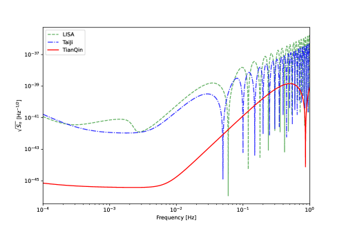
Figure 11: Noise PSD of TDI $A$ channel for LISA, TaiJi, and TianQin (four year data).

In Fig. 11, we have shown the three noise PSD curves of TDI 1 generation $A$ channel for LISA, TaiJi, and TianQin.

VI Waveform

In order to extract information from the detector data, one should model the entire detection process. With the basic definition in section IV.1, one can build a model for some general GW signals. To know the type of GW source and more information about the GW systems, an exact waveform is needed. In this section, we review some waveforms we use for each type of the source.

VI.1 Galaxy Compact Binary

In the mHz frequency band, GW events are mainly composed of white dwarf binaries (WDBs) in the Milky Way (with the number $\sim\mathcal{O}(10^{8})$) Nelemans et al. (2001), which are expected to be the most numerous GW sources for SBD. These GCBs are expected to exhibit relatively little frequency evolution. Thus, the GW strain emitted from a GCB can be safely approximated as (in the source frame) Katz et al. (2022)

$$h_{+}(t)= A_{+}\cos\Phi(t)=h_{0}\frac{1+\cos^{2}\iota}{2}\cos\Phi(t),$$ (122)

$$h_{\times}(t)= A_{\times}\sin\Phi(t)=h_{0}\cos\iota\sin\Phi(t),$$ (123)

$$h_{0}= \frac{4(G\mathcal{M}_{c})^{5/3}}{c^{4}D_{L}}(\pi f)^{2/3},$$ (124)

$$\Phi(t)= 2\pi ft+\pi\dot{f}t^{2}+\frac{\pi}{3}\ddot{f}t^{2}+\phi_{0},$$ (125)

where $\iota$ is the inclination angle of the quadruple rotation axis with respect to the line of sight (here the direction is from the source to the Sun), $\mathcal{M}_{c}=(m_{1}m_{2})^{3/5}/(m_{1}+m_{2})^{1/5}$ is the chirp mass of the system ($m_{1}$ and $m_{2}$ are the individual masses of the components of the binary), $D_{L}$ is the luminosity distance to the source, $\phi_{0}$ is the initial phase at the start of the observation, $f$, $\dot{f}$ and $\ddot{f}$ are the frequency of the source, frequency’s derivative, and double derivative with respect to time, and $\ddot{f}=\frac{11}{3}\frac{\dot{f}^{2}}{f^{2}}$.

Considering the motion of the detectors moving around the Sun, a Doppler modulation of the phase of the waveform should be taken into account, i.e.,

$$\Phi(t) \rightarrow\Phi(t)+\Phi_{D}(t),$$ (126)

$$\Phi_{D}(t) =2\pi(f+\dot{f}t)\,\frac{R}{c}\cos\beta\cos(2\pi f_{m}t-\lambda),$$ (127)

where $\Phi_{D}(t)$ is the Doppler modulation, $f_{m}=1/$year is the modulation frequency, $\beta$ and $\lambda$ are the latitudes and the longitude of the source in ecliptic coordinates, $R$=1AU is the semi-major axis of the guiding centre of the satellite constellation, respectively.

VI.2 Black Hole Binary

General Phenomenological waveform

For a black hole binariy (BHB) system, one can describe its waveform in the time domain or frequency domain with the help of stationary phase approximation. Here, we consider the frequency domain IMRPhenomD waveform, which assumes aligned spin so only two parameters are needed in describing the spin parameters Khan et al. (2016); Husa et al. (2016). In this frame, a BHB system can be characterized by four intrinsic parameters: masses $(m_{1},m_{2})$ and dimensionless spins $(\chi_{1},\chi_{2})$; seven extrinsic parameters: luminosity distance $D_{L}$, inclination angle $\iota$, polarization angle $\psi$, coalescence time and phase $(t_{c},\phi_{c})$ and the ecliptic longitude and ecliptic latitude $(\lambda,\beta)$ in the SSB. In the IMRPhenomD waveform model, the waveform of plus and cross mode will be

$${\tilde{h}}_{+}(f)= \frac{\mathcal{M}_{c}^{5/6}}{\pi^{2/3}D_{L}}\frac{1+\cos^{2}\iota}{2}f^{-7/6}\exp(\mathrm{i}\Psi(f)),$$ (128)

$${\tilde{h}}_{\times}(f)= -\mathrm{i}\frac{M_{c}^{5/6}}{\pi^{2/3}D_{L}}\cos{\iota}\,f^{-7/6}\exp(\mathrm{i}\Psi(f)).$$

More details about the phase $\Psi(f)$ can be seen in Khan et al. (2016).

Eccentric waveform

The GW emission causes the circularization effect, which makes the binaries almost non-eccentric when they are in the GBD frequency band. But when the binaries are in the SBD frequency band the eccentricity should be taken into account. Many eccentric waveform models have been developed to dateLoutrel (2020). Here we use EccentricFD, which is a frequency-domain third post-Newtonian (3PN) waveform with initial eccentricity $e_{0}$ valid up to 0.4 Yunes et al. (2009); Huerta et al. (2014), and has been included into LALSuiteLIGO Scientific Collaboration (2018). This analytic model only contains the inspiral process of a binary, however, it is sufficient for SBHBs, as they are likely to merge outside the sensitive frequency band of SBDs.

Note that, the BHB system can be divided into MBHB and SBHB systems according to their masses and origin. The heavier BHB systems have lower frequency bands. Though their origin or characterize are different, their waveform formulas are similar. When analysing the data, it is important to note the range of parameter values and the applicability of the waveform.

VI.3 Extreme Mass Ratio Inspirals

To expedite the generation of EMRI signals, we utilize the FastEMRIWaveform (FEW) package. The FEW is optimized to generate gravitational wave signals efficiently with GPU acceleration Chua et al. (2021). A reduced-order-model technique is employed in actuality, reducing the number of harmonic modes needed by approximately 40 times and thereby significantly cutting down the time needed to generate the waveform for each source Chua et al. (2021). For example,$l\in[2,10]$,$m\in[0,l]$ and $n\in[-30,30]$,which totals 3843 modes reduce to $\sim 10^{2}$ modes. The fully relativistic FEW model is limited to eccentric orbits in the Schwarzschild spacetime.

In specific, the time domain dimensionless strain of an EMRI source $h(t)$ can be given by

$$h(t)=\frac{\mu}{d_{L}}\sum_{lmkn}A_{lmkn}(t)S_{lmkn}(t,\theta)e^{im\phi}e^{-i\Phi_{mkn}(t)},$$ (129)

where $t$ is the time of arrival of the gravitational wave at the solar system barycenter, $\theta$ is the source-frame polar viewing angle, $\phi$ is the source-frame azimuthal viewing angle, $d_{L}$ is the luminosity distance, and $\{l,m,k,n\}$ are the indices describing the frequency-domain harmonic mode decomposition. The indices $l,m,k$, and $n$ label the orbital angular momentum, azimuthal, polar, and radial modes, respectively. $\Phi_{mkn}=m\Phi_{\varphi}+k\Phi_{\theta}+n\Phi_{r}$ is the summation of decomposed phases for each given mode. The amplitude $A_{lmkn}$ is related to the amplitude $Z_{lmkn}^{\infty}$ of the Teukolsky mode amplitude far from the source. It is given by $A_{lmkn}=-2Z_{lmkn}^{\infty}/\omega_{mkn}^{2}$, where $\omega_{mkn}=m\Omega_{\varphi}+k\Omega_{\theta}+n\Omega_{r}$ is the frequency of the mode, and $\Omega_{r,\theta,\phi}$ describe the frequencies of a Kerr geodesic orbit.

VI.4 Stochastic Gravitational Waves Background

In addition to the aforementioned primary distinguishable GW sources, there is another important type of GW source that could potentially be detected by SBD, known as the SGWB. SGWB is composed by a huge number of independent and unresolved GW sources Romano and Cornish (2017). These stochastic signals are effectively another source of noise in GW detectors. A SGWB can be written as a superposition of plane waves with frequencies of $f$ and coming from different directions ${\hat{k}}$ on the sky

$$h_{ij}(t,{\bf x})=\sum_{P}\int_{-\infty}^{+\infty}df\int_{S^{2}}d\Omega_{{\hat{k}}}{\tilde{h}}_{P}(f,{\hat{k}})e^{P}_{ij}(\hat{k})e^{\mathrm{i}2\pi f[t-{\hat{k}}\cdot{\bf x}(t)/c]},$$ (130)

where $P=\{+,\times\}$ denotes polarization. As a stochastic source, one can treat the complex amplitude ${\tilde{h}}_{P}(f,{\hat{k}})$ as some random variable with zero mean value. Supposing the SGWB is stationary, Gaussian, isotropic, and unpolarized, the ensemble average of the two random amplitudes ${\tilde{h}}_{P}(f,k)$ can be defined as Romano and Cornish (2017); Allen and Romano (1999)

$$\langle{\tilde{h}}_{P}(f,\hat{k}){\tilde{h}}^{*}_{P^{\prime}}(f^{\prime},\hat{k}^{\prime})\rangle=\delta(f-f^{\prime})\frac{\delta^{2}({\hat{k}},{\hat{k}}^{\prime})}{4\pi}\delta_{PP^{\prime}}\frac{1}{2}S_{h}(f).$$ (131)

The function $S_{h}(f)$ is the one-sided PSD of SGWB.

Note here that $\delta^{2}({\hat{k}},{\hat{k}}^{\prime})$ is a Dirac delta over the two-sphere, and it implies that the SGWB is independent of ${\hat{k}}$. However, it is expected that the SBDs will detect millions of WDBss in the Milky Way and nearby universe Seoane et al. (2023), and the superposition of millions of unresolved WDBss will contribute to an SGWB Rieck et al. (2023) (often referred to as foreground due to its strength). Furthermore, due to our location at one end of the Milky Way, this SGWB is anisotropic. Of course, there may exist other anisotropic SGWBs as well Bartolo et al. (2022). In this case, the PSD of the anisotropic SGWB will depend on the frequency and direction as $\mathscr{P}(f,{\hat{k}})$. If we assume SGWB is directional and frequency independent, the PSD can be factorized as Allen and Ottewill (1997)

$$\mathscr{P}(f,\hat{k})=H(f)\mathcal{P}_{h}(\hat{k})$$ (132)

where the PSD of the SGWB is given by $H(f)$, and the $\mathcal{P}_{h}(\hat{k})$ describes the distribution of signal.

VII Example data-set

In order to simulate the joint observation of certain GW signals, it is necessary to have precise knowledge of the relative positions of the three detector. The relative positions of guiding centers for each detector can be determined by the initial phase parameter $\alpha-\beta$ or $\kappa_{0}$ and $\alpha^{\prime\prime}$ as defined in Eqs. (17)-(19) and Eqs. (23)-(25). Additionally, the relative position of the spacecrafts in different detectors can be determined by the initial phase of the spacecraft (here is the initial phase parameter $\lambda$ and $\lambda^{\prime}$). Once the detector are launched, the relative pahse and positions are fixed. However, when simulating data for testing purposes, the initial phase parameters are some arbitrary values.

MBHB are the primary sources for SBDs, and its total inspiral-merger-ringdown phase can be detected in the mHz band. In Fig. 12, we have shown the MBHB event detected by TianQin, LISA and TaiJi and relative noise PSD. From the figure, it can be found that the length of the arms gives LISA and TaiJi an advantage in terms of the response intensity to signals, but at the same time, it also results in higher low-frequency noise levels.

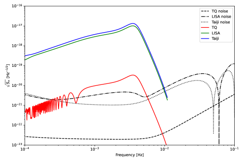
Figure 12: TDI-A channel responsed MBHB signal and relative noise PSD detected by different detectors. The masses for the binary system are ($3.5\times 10^{6},2.1\times 10^{5}$) $M_{\odot}$, spins are $(0.2,0.1)$, the luminosity distance is $10^{3}$ Mpc, the position is $(\lambda,\beta)=(0.4,1.2)$, and $\iota=0.3,t_{c}=0$. The total observation time is three months. Here the IMRPhenomD waveform is applied. The initial phase of TianQin’s and LISA’s first spacecraft is set to 0 for this figures.

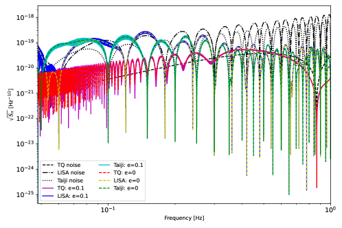
Figure 13: TDI-A channel responsed SBHB signal and relative noise PSD detected by different detectors. The masses for the binary system are ($35.6,30.6$) $M_{\odot}$, the luminosity distance is $100$ Mpc, the position is $(\lambda,\beta)=(4.7,-1.5)$, and $\iota=0.3,t_{c}=0$. The total observation time is three months. Here we have usde the EccentricFD waveform. The initial phase of TianQin’s and LISA’s first spacecraft is set to 0 for this figures.

The mass of SBHB systems is relatively lighter compared to MBHB, which leads to these systems predominantly producing signals in higher frequency ranges. In the Fig. 13, we can observe the performance of a SBHB signal across different detectors. Interestingly, when eccentricity is taken into account, the response waveform becomes considerably more intricate compared to the case where eccentricity is disregarded. This increased complexity in the waveform poses significant challenges for data processing and analysis. Furthermore, the figure demonstrates that the intersection point between the curve of the response signal from TianQin and the noise PSD is noticeably higher than in the case of LISA or TaiJi. This observation suggests that TianQin exhibits certain advantages in high-frequency detection.

In the low-frequency region of Fig. 12, the post-response signal of TianQin shows oscillations. Likewise, in Fig 13, the response signals from all three detectors demonstrate oscillatory behaviour. These oscillations arise as a result of the orbital motion of the detectors.

VIII Summary

Around 2035, one may see more than one SBDs operating simultaneously, with potential candidates include TianQin, LISA and TaiJi. Apart from the huge prospect on the scientific return from the joint observation over single detectors Torres-Orjuela et al. (2023), there are also challenges to doing data analysis for joint observation. In order to facilitate the study of problems involved in the joint data analysis, we have introduced GWSpace in this paper, which is a package that can simulate the joint detection data from three SBDs: TianQin, LISA and TaiJi.

GWSpace uses SSB as the common coordinate system for all detectors. It can simulate data for GCB, BHB, EMRI, SGWB, and simple burst signals. It supports injecting time-domain waveform functions and obtaining observed data through time-domain responses. For frequency-domain waveforms, it supports the frequency-domain responses of regular 22 mode, higher harmonic modes, and waveforms with eccentricity BHB. The TDI 1st combinations in time domain and frequency domain now are included. It includes the time-domain and frequency-domain responses of the 1st generation TDI combinations, and the corresponding TDI noise. We have also given a few example data set generated with the package. The package is open source and is free for downloading from this GWSpace. To clearly define all the notations and to eliminate possible misunderstanding, we have presented a detailed description of the coordinate system, the detector orbits, the detector responses, the TDI combinations, the instrumental noise models, and the waveforms for each source in this paper.

As the first work in this direction, GWSpace can be further improved in many ways. For example, we have only implemented the first generation TDI so far while second generation combinations are usually required, at least for LISA and Taiji. What’s more, more robust response is needed for some sources with complex waveforms, such as BHB systems with eccentricity Wang et al. (2023). The package is still relaying on very idealistic assumption about the noise: the noises from all satellites in a detector are identical, while in reality no two spacecraft can be exactly the same Cheng et al. (2022).

One can improve on the last point by implementing more sophisticated noise models for each detectors, but the most precise noise model will have to come from people responsible for each detector. We are hopeful that this may happen one day, and then GWSpace can serve as the starting point for a serious multi-mission data challenge for space-based GW detection.

References

- Luo et al. (2016) J. Luo, L.-S. Chen, H.-Z. Duan, Y.-G. Gong, S. Hu, J. Ji, Q. Liu, J. Mei, V. Milyukov, M. Sazhin, et al. (TianQin), Class. Quant. Grav. 33, 035010 (2016), eprint 1512.02076.
- Danzmann (1997) K. Danzmann, Class. Quant. Grav. 14, 1399 (1997).
- Amaro-Seoane et al. (2017) P. Amaro-Seoane et al. (LISA) (2017), eprint 1702.00786.
- Gong et al. (2015) X. Gong et al., J. Phys. Conf. Ser. 610, 012011 (2015), eprint 1410.7296.
- Hu and Wu (2017) W.-R. Hu and Y.-L. Wu, Natl. Sci. Rev. 4, 685 (2017).
- Abbott et al. (2021) R. Abbott et al. (LIGO Scientific, VIRGO, KAGRA) (2021), eprint 2111.03606.
- Huang et al. (2020) S.-J. Huang, Y.-M. Hu, V. Korol, P.-C. Li, Z.-C. Liang, Y. Lu, H.-T. Wang, S. Yu, and J. Mei, Phys. Rev. D 102, 063021 (2020), eprint 2005.07889.
- Lu et al. (2023) Y. Lu, E.-K. Li, Y.-M. Hu, J.-d. Zhang, and J. Mei, Res. Astron. Astrophys. 23, 015022 (2023), eprint 2205.02384.
- Wang et al. (2019) H.-T. Wang et al., Phys. Rev. D 100, 043003 (2019), eprint 1902.04423.
- Liu et al. (2020) S. Liu, Y.-M. Hu, J.-d. Zhang, and J. Mei, Phys. Rev. D 101, 103027 (2020), eprint 2004.14242.
- Wang et al. (2023) H. Wang, I. Harry, A. Nitz, and Y.-M. Hu (2023), eprint 2304.10340.
- Fan et al. (2020) H.-M. Fan, Y.-M. Hu, E. Barausse, A. Sesana, J.-d. Zhang, X. Zhang, T.-G. Zi, and J. Mei, Phys. Rev. D 102, 063016 (2020), eprint 2005.08212.
- Zhang et al. (2022) X.-T. Zhang, C. Messenger, N. Korsakova, M. L. Chan, Y.-M. Hu, and J.-d. Zhang, Phys. Rev. D 105, 123027 (2022), eprint 2202.07158.
- Liang et al. (2022) Z.-C. Liang, Y.-M. Hu, Y. Jiang, J. Cheng, J.-d. Zhang, and J. Mei, Phys. Rev. D 105, 022001 (2022), eprint 2107.08643.
- Cheng et al. (2022) J. Cheng, E.-K. Li, Y.-M. Hu, Z.-C. Liang, J.-d. Zhang, and J. Mei, Phys. Rev. D 106, 124027 (2022), eprint 2208.11615.
- Seoane et al. (2023) P. A. Seoane et al. (LISA), Living Rev. Rel. 26, 2 (2023), eprint 2203.06016.
- Arun et al. (2022) K. G. Arun et al. (LISA), Living Rev. Rel. 25, 4 (2022), eprint 2205.01597.
- Auclair et al. (2023) P. Auclair et al. (LISA Cosmology Working Group), Living Rev. Rel. 26, 5 (2023), eprint 2204.05434.
- Baker et al. (2022) T. Baker et al. (LISA Cosmology Working Group), JCAP 08, 031 (2022), eprint 2203.00566.
- Bartolo et al. (2022) N. Bartolo et al. (LISA Cosmology Working Group), JCAP 11, 009 (2022), eprint 2201.08782.
- Belgacem et al. (2019) E. Belgacem et al. (LISA Cosmology Working Group), JCAP 07, 024 (2019), eprint 1906.01593.
- Babak et al. (2010) S. Babak et al. (Mock LISA Data Challenge Task Force), Class. Quant. Grav. 27, 084009 (2010), eprint 0912.0548.
- Baghi (2022) Q. Baghi (LDC Working Group), in 56th Rencontres de Moriond on Gravitation (2022), eprint 2204.12142.
- Ren et al. (2023) Z. Ren, T. Zhao, Z. Cao, Z.-K. Guo, W.-B. Han, H.-B. Jin, and Y.-L. Wu, Front. Phys. (Beijing) 18, 64302 (2023), eprint 2301.02967.
- Arnaud et al. (2007) K. A. Arnaud, G. Auger, S. Babak, J. G. Baker, M. J. Benacquista, E. Bloomer, D. A. Brown, J. Camp, J. Cannizzo, N. Christensen, et al., Classical and Quantum Gravity 24, S529 (2007).
- Babak et al. (2008) S. Babak et al. (Mock LISA Data Challenge Task Force), Class. Quant. Grav. 25, 114037 (2008), eprint 0711.2667.
- Gong et al. (2021) Y. Gong, J. Luo, and B. Wang, Nature Astron. 5, 881 (2021), eprint 2109.07442.
- Crowder and Cornish (2005) J. Crowder and N. J. Cornish, Phys. Rev. D 72, 083005 (2005), eprint gr-qc/0506015.
- Ruan et al. (2020) W.-H. Ruan, C. Liu, Z.-K. Guo, Y.-L. Wu, and R.-G. Cai, Nature Astron. 4, 108 (2020), eprint 2002.03603.
- Wang et al. (2020) G. Wang, W.-T. Ni, W.-B. Han, S.-C. Yang, and X.-Y. Zhong, Phys. Rev. D 102, 024089 (2020), eprint 2002.12628.
- Zhu et al. (2022) L.-G. Zhu, L.-H. Xie, Y.-M. Hu, S. Liu, E.-K. Li, N. R. Napolitano, B.-T. Tang, J.-d. Zhang, and J. Mei, Sci. China Phys. Mech. Astron. 65, 259811 (2022), eprint 2110.05224.
- Lyu et al. (2023) X. Lyu, E.-K. Li, and Y.-M. Hu (2023), eprint 2307.12244.
- Liang et al. (2023a) Z.-C. Liang, Z.-Y. Li, J. Cheng, E.-K. Li, J.-d. Zhang, and Y.-M. Hu, Phys. Rev. D 107, 083033 (2023a), eprint 2212.02852.
- Liang et al. (2023b) Z.-C. Liang, Z.-Y. Li, E.-K. Li, J.-d. Zhang, and Y.-M. Hu (2023b), eprint 2307.01541.
- Schutz (2011) B. F. Schutz, Class. Quant. Grav. 28, 125023 (2011), eprint 1102.5421.
- Torres-Orjuela et al. (2023) A. Torres-Orjuela, S.-J. Huang, Z.-C. Liang, S. Liu, H.-T. Wang, C.-Q. Ye, Y.-M. Hu, and J. Mei (2023), eprint 2307.16628.
- Xie et al. (2023) Y. Xie, D. Chatterjee, G. Holder, D. E. Holz, S. Perkins, K. Yagi, and N. Yunes, Phys. Rev. D 107, 043010 (2023), eprint 2210.09386.
- Roulet et al. (2022) J. Roulet, S. Olsen, J. Mushkin, T. Islam, T. Venumadhav, B. Zackay, and M. Zaldarriaga, Phys. Rev. D 106, 123015 (2022), eprint 2207.03508.
- Cutler (1998) C. Cutler, Phys. Rev. D 57, 7089 (1998), eprint gr-qc/9703068, URL https://link.aps.org/doi/10.1103/PhysRevD.57.7089.
- Marsat and Baker (2018) S. Marsat and J. G. Baker, arXiv:1806.10734 [gr-qc] (2018), arXiv: 1806.10734, eprint 1806.10734, URL http://arxiv.org/abs/1806.10734.
- Marsat et al. (2021) S. Marsat, J. G. Baker, and T. Dal Canton, Phys. Rev. D 103, 083011 (2021), publisher: American Physical Society, eprint 2003.00357, URL https://link.aps.org/doi/10.1103/PhysRevD.103.083011.
- Chen et al. (2023) H.-Y. Chen, X.-Y. Lyu, E.-K. Li, and Y.-M. Hu (2023), eprint 2309.06910.
- Hu et al. (2018) X.-C. Hu, X.-H. Li, Y. Wang, W.-F. Feng, M.-Y. Zhou, Y.-M. Hu, S.-C. Hu, J.-W. Mei, and C.-G. Shao, Class. Quant. Grav. 35, 095008 (2018), eprint 1803.03368.
- Rubbo et al. (2004) L. J. Rubbo, N. J. Cornish, and O. Poujade, Phys. Rev. D 69, 082003 (2004), eprint gr-qc/0311069.
- Jolien D. E. Creighton (2011) W. G. A. Jolien D. E. Creighton, Gravitational Waves (John Wiley & Sons, Ltd, 2011), chap. 3, pp. 49–95, ISBN 9783527636037, eprint https://onlinelibrary.wiley.com/doi/pdf/10.1002/9783527636037.ch3, URL https://onlinelibrary.wiley.com/doi/abs/10.1002/9783527636037.ch3.
- Kogut et al. (1993) A. Kogut et al., Astrophys. J. 419, 1 (1993), eprint astro-ph/9312056.
- Goldberg et al. (1967) J. N. Goldberg, A. J. MacFarlane, E. T. Newman, F. Rohrlich, and E. C. G. Sudarshan, J. Math. Phys. 8, 2155 (1967).
- Yunes et al. (2009) N. Yunes, K. G. Arun, E. Berti, and C. M. Will, Phys. Rev. D 80, 084001 (2009), URL https://link.aps.org/doi/10.1103/PhysRevD.80.084001.
- Wahlquist (1987) H. Wahlquist, Gen. Rel. Grav. 19, 1101 (1987).
- Armstrong et al. (1999) J. W. Armstrong, F. B. Estabrook, and M. Tinto, The Astrophysical Journal 527, 814 (1999), ISSN 0004-637X, aDS Bibcode: 1999ApJ…527..814A, URL https://ui.adsabs.harvard.edu/abs/1999ApJ...527..814A.
- Katz et al. (2022) M. L. Katz, J.-B. Bayle, A. J. K. Chua, and M. Vallisneri, Phys. Rev. D 106, 103001 (2022), eprint 2204.06633.
- Estabrook and Wahlquist (1975) F. B. Estabrook and H. D. Wahlquist, General Relativity and Gravitation 6, 439 (1975).
- Romano and Cornish (2017) J. D. Romano and N. J. Cornish, Living Rev. Rel. 20, 2 (2017), eprint 1608.06889.
- Cornish and Rubbo (2003) N. J. Cornish and L. J. Rubbo, Phys. Rev. D 67, 022001 (2003), [Erratum: Phys.Rev.D 67, 029905 (2003)], eprint gr-qc/0209011.
- Tinto and Dhurandhar (2021) M. Tinto and S. V. Dhurandhar, Living Rev. Rel. 24, 1 (2021), ISSN 1433-8351, URL https://doi.org/10.1007/s41114-020-00029-6.
- Prince et al. (2002) T. A. Prince, M. Tinto, S. L. Larson, and J. W. Armstrong, Phys. Rev. D 66, 122002 (2002), publisher: American Physical Society, eprint gr-qc/0209039, URL https://link.aps.org/doi/10.1103/PhysRevD.66.122002.
- Babak et al. (2021) S. Babak, A. Petiteau, and M. Hewitson (2021), eprint 2108.01167.
- Nelemans et al. (2001) G. Nelemans, L. R. Yungelson, and S. F. Portegies Zwart, Astron. Astrophys. 375, 890 (2001), eprint astro-ph/0105221.
- Khan et al. (2016) S. Khan, S. Husa, M. Hannam, F. Ohme, M. Pürrer, X. Jiménez Forteza, and A. Bohé, Phys. Rev. D 93, 044007 (2016), eprint 1508.07253, URL https://link.aps.org/doi/10.1103/PhysRevD.93.044007.
- Husa et al. (2016) S. Husa, S. Khan, M. Hannam, M. Pürrer, F. Ohme, X. Jiménez Forteza, and A. Bohé, Phys. Rev. D 93, 044006 (2016), eprint 1508.07250, URL https://link.aps.org/doi/10.1103/PhysRevD.93.044006.
- Loutrel (2020) N. Loutrel, arXiv e-prints arXiv:2009.11332 (2020), eprint 2009.11332.
- Huerta et al. (2014) E. A. Huerta, P. Kumar, S. T. McWilliams, R. O’Shaughnessy, and N. Yunes, Phys. Rev. D 90, 084016 (2014), URL https://link.aps.org/doi/10.1103/PhysRevD.90.084016.
- LIGO Scientific Collaboration (2018) LIGO Scientific Collaboration, LIGO Algorithm Library - LALSuite, free software (GPL) (2018).
- Chua et al. (2021) A. J. K. Chua, M. L. Katz, N. Warburton, and S. A. Hughes, Phys. Rev. Lett. 126, 051102 (2021), eprint 2008.06071.
- Allen and Romano (1999) B. Allen and J. D. Romano, Phys. Rev. D 59, 102001 (1999), eprint gr-qc/9710117.
- Rieck et al. (2023) S. Rieck, A. W. Criswell, V. Korol, M. A. Keim, M. Bloom, and V. Mandic (2023), eprint 2308.12437.
- Allen and Ottewill (1997) B. Allen and A. C. Ottewill, Phys. Rev. D 56, 545 (1997), eprint gr-qc/9607068.