School Bus Routing Problem with Open Offer Policy: incentive pricing strategy for students that opt-out using school bus

Abstract

This work introduces the School Bus Routing Problem with Open Offer Policy (SBRP-OOP) motivated by the Williamsville Central School District (WCSD) of New York. School districts are often mandated to provide transportation, but students assigned to the buses commonly do not use the service. Consequently, buses frequently run with idle capacity over long routes. The SBRP-OOP seeks to improve capacity usage and minimize the bus fleet by openly offering a monetary incentive to students willing to opt-out of using a bus. Then, students who certainly will not take a bus due to acceptance of the incentive are not included in the routing generation. Mathematical formulations are proposed to determine a pricing strategy that balances the trade-off between incentive payments and savings obtained from using fewer buses. The effectiveness of the Open Offer Policy approach is evaluated for instances from a real operational context in New York.

Keywords: School bus routing; Pricing strategy; Overbooking, Simulation, Integer programming; Column generation; Heuristics

1 Introduction

School Bus Routing Problem (SBRP) is part of the family of Vehicle Routing Problem (VRP), in which a set of school bus routes has to be determined in order to pick up a given set of students from a set of potential bus stops and transporting them to the school. The SBRP is cost-intensive for school administrators [Ellegood et al., 2019]; therefore, improving transportation efficiency releases school resources that can be used to enhance educational programs, build new infrastructure, and increase teachers’ wages, among others.

Most SBRP publications focus on minimizing the length or cost of routes, constrained to all students to be assigned to a bus [Park and Kim, 2010]. However, recent works have shifted the characteristics being examined to emphasize the real issues of the SBRP [Ellegood et al., 2019]. For example, although overbooking strategies are typically used in practical school bus routing problems, they have yet to be approached in the literature. Recently, in [Caceres et al., 2017] has been introduced an overbooking strategy for the SBRP to improve the seat utilization of buses due to some students not using the service.

A commonly used policy in school districts is to assign every student to a bus route, regardless of whether they decide to ride the bus. Also, there is no incentive to actively opt-out, i.e., to notify the school district that a student will not use a bus. However, if students not using the school bus system were to opt-out at the beginning of the school year, motivated by a monetary incentive, the district could design a smaller set of routes only for those students who actually use the bus.

In this paper, we introduce a new family of SBRP called School Bus Routing Problem with Open Offer Policy (SBRP-OOP). The SBRP-OOP seeks to determine a pricing strategy to balance incentive payments to the students willing to opt-out of using a bus and the savings obtained from using fewer buses to pick up students from their assigned stops. Students that accept the incentive are not considered in the routing generation process. Then, we consider an SBRP with a single school whose objective is to simultaneously: i) find the set of stops to visit from a set of potential stops, ii) assign each student to a stop, considering a maximum total distance that a student has to walk and a maximum number of students per stop, and iii) generate routes to visit the selected stops; such that the total distance traveled by buses is minimized.

1.1 Problem motivation

The SBRP-OOP is motivated by the Williamsville Central School District (WCSD) operational context, belonging to the New York State Education Department. School bus transportation in New York State is free and must be provided to all students by law. WCSD policy states that all students must be assigned to a stop, and all stops must be visited despite the uncertainty of students not showing up. Consequently, the district finds itself reliant on a large fleet of buses, many of which are underutilized. This situation incurs significant expenses in terms of bus maintenance and driver salaries, leading to excessive costs.

Moreover, the WCSD is grappling with a severe shortage of bus drivers, a problem that the COVID-19 pandemic has exacerbated, according to local media [Desmond, 2022]. Prospective candidates, typically retirees, harbor skepticism about working in close proximity to children and often prefer work-from-home or package delivery positions [Lando, 2023]. As a result, the district is confronted with great challenges in both fleet reduction to achieve cost savings and ensuring an adequate number of personnel to meet the demands of its bus transportation system.

Students can choose on any day whether they want to access bus transportation. We know that up to 80% of the students use the transportation provided by the district [Caceres et al., 2017]. By studying the data gathered daily at the district, we found that the likelihood of a student using the bus is highly correlated to i) the kind of school attended (elementary school, middle school, or high school), and ii) the bus schedule (morning or afternoon).

We define ridership as the ratio between the number of students riding a bus and the total number assigned to it. Figure 1 shows the ridership for each school, separating the AM and PM cases. We can see how no more than 80% of the students use the transportation the school district provides. The fact that these students are still assigned to a bus accounts for longer routes and low capacity usage.

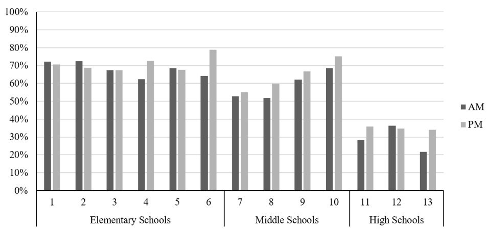
Figure 1: Average ridership per school and level.

The WCSD uses an overbooking policy to utilize bus capacities better. By reviewing routes yearly, the district determines whether to update overbooking limits, provided the information on actual ridership is available. With this information, the number of assigned students to a bus is determined so that it is improbable have an event of overcrowding. However, if such an event occurs, it would do in the school’s proximity, near the end of the route and close to the bell time; therefore, the students would simply be squeezed into any seat. Finally, saving opportunities for the WCSD come mainly from reducing the maximum number of buses being used simultaneously at any given time during the day. The need for an additional bus implies either hiring a driver and purchasing a new bus or paying the contractor for another bus. Both these options are expensive. Like in Boston, MA Bertsimas et al. [2020], in Williamsville, NY, most transportation costs are driven by the total number of buses operating every day.

Given this operational context, we propose a different approach to improve capacity usage. We explore the effect of encouraging students to opt-out of school buses to reduce the fleet size used for the school district. We call this problem the School Bus Routing Problem with Open Offer Policy (SBRP-OOP). An Open Offer Policy will try to reduce the number of students using the school buses through a monetary incentive. This policy aims to offer an incentive openly, extended as a check or a tax return, to any student willing to opt-out of using a bus. This incentive is determined before students decide whether to accept the deal. In this policy, the school district does not control which students would accept the offer but only controls the incentive’s value. Thus, the incentive value needs to be determined in such a manner that it should reduce the possibility of having to pay more for incentives than what would be saved by using fewer buses.

Figure 2 illustrates the fleet reduction. Figure 2(a) describes an instance of the problem with one school (represented by the black square), a set of potential stops (represented by the small white square), and the set of students with the stops that they are able to reach (represented by the black dots and the dotted lines, respectively). Figure 2(b) describes a possible solution for the traditional SBRP with bus stop selection (SBRP-BSS) when the bus capacity is equal to 6. This potential solution uses three routes (represented by the blue lines), visiting seven stops to ride the students. Finally, Figure 2(c) describes a possible solution for the SBRP-OOP, considering the same bus capacity. We can observe that three students accepted the incentive for opt-out of using the buses (represented by the red dots). Therefore, these three students are not considered in the route planning process. In comparison to the traditional SBRP-BSS approach, it is evident that only two routes are utilized to serve five stops and transport the students. Consequently, the school district can accomplish this with just two buses, reducing the idle capacity. It is important to note that this scenario proves advantageous for the school district only if the cost savings resulting from using fewer buses outweigh the total amount spent on incentives provided to the students who have accepted the opt-out offer.

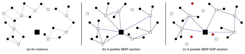
Figure 2: Motivation example for the SBRP-OOP

1.2 Our contribution

This paper makes three distinct contributions.

Firstly, we introduce the SBRP with an open offer policy, which aims to reduce the fleet size required for transporting students to their schools by providing economic incentives for students to opt-out of the system. Additionally, we define key performance indicators, specifically focusing on the probability of failure, to evaluate the effectiveness of pricing policies.

Secondly, we propose a simulation-based solution method to estimate the indicators associated with a single school. To achieve this, we present two optimization problems that allocate the ridership level and the opt-out probability among the students while maintaining the school’s original average parameter. Subsequently, we simulate the opt-out process based on the obtained probabilities and solve the routing problem to determine the minimum fleet required for students who decline the economic incentive.

Lastly, we conduct tests using both synthetic and real instances. With synthetic data, we discover that the open offer policy proves advantageous when students are concentrated in proximity to their schools. When examining real data from the WCSD, we observe that the open offer policy has potential implementation in middle schools, even with substantial economic incentives of up to $1500 USD from the students that decide to opt-out the system.

1.3 Roadmap

The remainder of this paper is organized as follows. Section 2 gives a literature review of the SBRP with bus stop selection. Section 3 presents a mathematical formulation of the problem considering overbooking. Section 4 describes our solution framework for the SBRP-OOP. Section 5 reports the results of computational experiments. Finally, Section 6 presents the conclusions.

2 Literature review

The School Bus Routing Problem (SBRP) was introduced in Newton and Thomas [1969] and has been studied extensively. It consists of four interrelated sub-problems: the tactical bus stop selection sub-problem, the operational bus route generation, bus route scheduling, and school bell time adjustment sub-problems. The bus stop selection sub-problem seeks to determine a set of bus stops to visit and allocate each student to one of these bus stops, limiting the walking distance of the students by a given value. The bus route generation sub-problem is the central issue of the SBRP. It covers the decision to design the bus routes to visit the bus stops at the minimum cost without exceeding the bus capacity. The bus route scheduling sub-problem specifies each route’s starting and ending time and forms a chain of routes that can be executed sequentially by the same bus. Finally, the school bell time adjustment sub-problem considers school’s starting and ending times as decision variables and seeks to find the optimal times to maximize the number of routes served sequentially by the same bus and reduce the number of buses used.

In the literature, it is difficult to determine a dominant approach to solve the SBRP since all works propose different considerations, differing mainly in the sub-problems that are solved and the real-world characteristics considered. It is possible to observe that the latest studies emphasize real-world issues such as heterogeneous fleets, mixed loading, serving multiple schools, and ridership uncertainty (Ellegood et al. [2019]). The present review mainly focuses on works that solve the bus stop selection and bus route generation sub-problems, and explores how these works emphasize different real-world aspects. For a general review of the different classifications, objectives, and contemporary trends on SBRP, we recommend the reader to Park and Kim [2010], Ellegood et al. [2019].

Because of the complexity of solving bus stop selection and bus route generation sub-problems simultaneously, these problems have been solved sequentially. The heuristic solution approaches can be classified into: the location-allocation-routing (LAR) strategy and the allocation-routing-location (ARL) strategy (Park and Kim [2010]).

The LAR strategy determines a set of bus stops for a school and allocates students to these stops. Then, routes are generated for the selected stops. The main drawback of this strategy is that it tends to create excessive routes because vehicle capacity constraints are ignored in the location-allocation phase (Bowerman et al. [1995]). The main papers that use a heuristic approach based on the LAR strategy are Bodin and Berman [1979], Dulac et al. [1980], Li and Chow [2021], Farzadnia and Lysgaard [2021], Calvete et al. [2021]. In Bodin and Berman [1979] the bus route scheduling sub-problem with mixed loads is additionally considered. The objective is to minimize the transportation cost, which consists of a fixed cost for each vehicle, the total routing cost, and the transportation time for each student. An ad-hoc heuristic approach is proposed to solve the problem with constraints on the maximum travel time for each student, a time window for arrival at the school, and the classical constraint on the maximum bus capacity. In Dulac et al. [1980] multiple schools are considered, but mixed loads are not allowed; therefore, the problem is solved for each school independently. The objective is to minimize the product between the number of routes and the sum of route lengths. An ad-hoc heuristic approach is proposed to solve the problem with constraints on the number of visited stops, the transportation time for each vehicle, and the distance walked by the student from the current potential stop to the selected bus stop. In Parvasi et al. [2017] the student’s choice to use alternative transportation systems is considered. A bi-level mathematical model is proposed considering the students are reluctant to choose any bus stops that are visited by a route and decide to use an alternative transportation system. At the upper-level, the decision concerning bus stops location is made, and routes buses to these stops are generated. Subsequently, the decision regarding the allocation of students to transportation systems or outsourcing them will be made at the lower level. Two hybrid metaheuristic approaches based on genetic algorithms, simulated annealing, and tabu search, are proposed to solve the model. In Li and Chow [2021] a mixed ride approach, where general and special education students are served on the same bus simultaneously while allowing heterogeneous fleets and mixed loads, is proposed. Here, mixed rides differ from mixed loads, which refers to buses serving students at different schools using the same bus. The goal is to reduce the route redundancy generated in a separate ride system when a general student and a special education student are at the same address but served by two different buses. Schools are divided into three types: (i) schools that only have general students; (ii) schools that only have special students; and (iii) mixed schools that have both general and special students. Then different strategies for bus stop selection are implemented for each type of school. ESRI Location-Allocation tools and Google OR-Tools are used for bus stop selection and route generation. In Farzadnia and Lysgaard [2021] the service-oriented single-route SBRP is considered. The approach focuses on providing good quality service for students who are sensitive and need more care and safety. Because walking distance is generally considered a quality service measure, the proposed model minimizes the total walking distance by students to the stop points, while treating the maximum total routing distance as a constraint. The problem considers a single school and a single route. In the bus route generation, it is assumed that a single vehicle with an unlimited capacity can pick up all students of one school who are eligible to ask for the bus. An exact and heuristic algorithm was developed. In Calvete et al. [2021] the SBRP with student choice is introduced. The work is an extension of Calvete et al. [2020] to study student’s reaction to the selection of bus stops when they are allowed to choose the bus stop that best suits them. A bilevel optimization model is formulated, considering the selection of the bus stops among the set of potential bus stops and the construction of the bus routes, considering both bus capacity and student preferences. A metaheuristic algorithm is developed to solve the problem in two steps. First, a subset of the set of potential bus stops is selected and allows the students to choose their preferred bus stop among the selected ones. Second, after knowing the number of students who take the bus at each bus stop, the routes are computed by solving the corresponding Capacited VRP and applying local search procedures.

The ARL strategy attempts to overcome the LAR strategy’s drawback, which tends to create excessive routes. First, the students are allocated into clusters while satisfying vehicle capacity constraints. Then, subsequently, the bus stops are selected, and a route is generated for each cluster. Finally, the students in a cluster (route) are assigned to a bus stop that satisfies all the problem requirements. The main drawback of this strategy is that the route length cannot be explicitly controlled because each route is generated after the allocation phase and depends on student’s dispersion within the individual clusters (Bowerman et al. [1995]). The main papers that use a heuristic approach based on the ARL strategy are Chapleau et al. [1985], Bowerman et al. [1995]. In Chapleau et al. [1985], as in Dulac et al. [1980], multiple schools are considered, but routes for each school are determined independently. The objective is to minimize the number of routes. An ad-hoc heuristic approach is proposed to solve the problem with constraints on the distance walked by the students, the number of stops on each route, and the length of each route. In Bowerman et al. [1995] a multi-objective optimization approach is introduced, which considers efficiency, effectiveness, and equity criteria. The objective is to minimize the number of routes and total bus route length (efficiency), student walking distance (effectiveness), and optimize both load and length balancing (equity). An ad-hoc heuristic approach is proposed to solve the problem with constraints on the bus capacity and maximum walking distance.

Bus stop selection and bus route generation are highly interrelated problems. They are treated separately in the previous works due to the complexity and size of the problems, but this generates sub-optimal solutions (Salhi and Rand [1989]). For this reason, recent studies have attempted to solve the problem through an integrated strategy (Riera-Ledesma and Salazar-González [2012, 2013], Schittekat et al. [2013], Kinable et al. [2014]). In Riera-Ledesma and Salazar-González [2012] the multiple vehicle traveling purchaser problem (MV-TPP) is introduced. The MV-TPP is a generalization of the vehicle routing problem and models a family of routing problems combining stop selection and bus route generation. The goal of the problem is to assign each user to a potential stop to find the least cost routes and choose a vehicle to serve each route so that a route serves each stop with assigned users. The objective is to minimize the total length of all routes plus the total user-stop assignment cost subject to capacity bus constraints. A Mixed Integer Programming (MIP) formulation is proposed, and a branch-and-cut algorithm is developed to solve the MIP. Later, an extension of this work is proposed in Riera-Ledesma and Salazar-González [2013]. Here, additional resource constraints on each bus route are considered: bounds on the distances traveled by the students, the number of visited bus stops, and the minimum number of students that a vehicle has to pick up. A branch-and-price algorithm with a set partitioning formulation is developed to solve the problem. In Schittekat et al. [2013] a matheuristic to solve large instances is proposed. The matheuristic consists of a construction phase, based on a GRASP metaheuristic, and an improvement phase based on a VND metaheuristic. The student allocation sub-problem is solved by modeling the problem as a transportation problem. Then, the problem is decomposed into a master problem and a sub-problem. The master problem is a school bus routing problem with bus stop selection, where the objective is to minimize the total traveled distance. Once the stops have been selected and the routes have been fixed, the sub-problem of allocating students to stops is solved so that the bus capacity is not exceeded. Additionally, a MIP formulation is proposed to compare the effectiveness of the matheuristic and a column generation approach is developed to compute lower bounds on the optimal solution. In Kinable et al. [2014] a branch-and-price framework based on a set covering formulation is proposed. The location of students is not provided but only is known for each student the set of stops to which this student can be assigned. Thus, no optimization of the student walking distances is required, but a maximum walking distance constraint is considered (propose an exact branch-and-price algorithm for the same problem). In Calvete et al. [2020] the same problem configuration as in Schittekat et al. [2013] is considered. But two main differences in the solution approach there exist: i) in the construction phase, it is proposed to integrate the allocation of the students and the route construction, while in Schittekat et al. [2013] the integrated sub-problems are the bus stop selection and the route generation, and ii) the procedure includes the solution of four purpose-built Mixed Integer Linear Programming (MILP) problems for selecting the bus stops, together with a more general random selection, which contributes to diversifying the considered solutions. The matheuristic developed is based on an approach that first partially allocates the students to a set of active stops they can reach and computes a set of routes that minimizes the routing cost. Then, a refining process is performed to complete the allocation and adapt the routes until a feasible solution is obtained.

All the articles cited have in common that they formulate the SBRP with deterministic demand; this means that the number of students requiring school bus service is known in advance and is the same every day. Under this assumption, bus capacity management is carried out considering different criteria, such as heterogeneous fleet, mixed loads, and mixed trips, in order to minimize the school bus’s travel distance and the cost of the fleet. In contrast to these deterministic models, we propose a stochastic approach in which the number of students traveling on a bus is unknown each day, taking into account the behavior of students not riding the bus on a given day. Therefore, with unknown ridership levels, it is necessary to extend the traditional criteria used in the literature for bus capacity management to avoid high idle capacity levels, unnecessarily increasing the transportation system’s costs. To reach this goal, we consider a strategy where students are compensated for giving up the option to ride a bus to reduce the overall cost of the system.

3 Mathematical formulations

Consider a school that offers a predefined incentive to any student willing to opt-out of using the school bus. We will focus on a pricing strategy to find a value for a monetary incentive $\tau$ such that the school district observes an overall reduction in transportation costs. That is to say, the saving on costs from reducing the number of routes must be more significant than the cost of paying the incentive $\tau$ to those students that decided to opt-out.

For each student $i\in A$, where $A=\{1,...,N\}$ is the set of all students, the variables $\mathscr{Y}_{i}$ are equal to 1 if student $i$ opt-out from riding the bus, and 0 otherwise. The variables $\mathscr{Y}_{i}$ are independently and identically distributed random variables that follow a Bernoulli distribution with parameter $r_{i}$, which represents the opt-out probability for student $i$. $\mathscr{R}\left(\forall i\in A:\mathscr{Y}_{i}=0\right)$ is the cost associated with routing the remaining students. Notice that $\mathscr{R}$ is also a random variable since it is a function of the random variables $\mathscr{Y}_{i},\forall i\in A$. Then, we aim to determine the value of the incentive $\tau$ to minimize the total expected transportation cost:

$$\mathscr{P}_{1}:\quad\min_{\tau}\quad E\left[\sum_{i\in A}\tau\mathscr{Y}_{i}+\mathscr{R}\left(\forall i\in A:\mathscr{Y}_{i}=0\right)\right]$$ (1)

An undesirable scenario for a district would be offering a certain incentive and observing students who opt-out not producing any routing savings. Alternatively, having reduced the fleet to a certain number of buses, another unfavorable event is realizing that those savings do not compensate for the total incentive given to the students that opted out. Let $\mathscr{K}$ represent the event “the savings due to fleet reduction do not compensate the cost of incentives for students”. Then, if the likelihood $r_{i}$ that each student accept an incentive $\tau$ is known, we would want to estimate the risk of a failed open offer policy given a particular value for $\tau$ as,

$$P\left(\mathscr{K}\;\middle|\;\tau\,,\,r_{i}\ \forall i\in A\right)=P\left(\sum_{i\in A}\tau\mathscr{Y}_{i}>\mathscr{R}\left(A\right)-\mathscr{R}\left(\forall i\in A:\mathscr{Y}_{i}=0\right)\;\middle|\;\tau\,,\,r_{i}\ \forall i\in A\right)$$ (2)

We refer to this as the probability of failre.

Moreover, it would be of value to find a range of $\tau$ for which the risk of a failed open offer policy is under a threshold. Let $R_{0}$ be the number of buses needed to route all students, and $R$ the number of buses to route students that do not opt-out. Let $\kappa$ be the total cost of operating one bus. And, let $X$ be the number of students that opted out. Then,

$$P\left(\mathscr{K}\;\middle|\;\tau\right) =\sum_{r}P\left(\kappa\left(R_{0}-R\right)<\tau X\;\middle|\;\tau,r\right)P(r)$$ (3)

$$=P\left(\kappa\Delta<\tau X\;\middle|\;r\right)$$ (4)

$$=P\left(\frac{X}{\Delta}>\frac{\kappa}{\tau}\;\middle|\;r\right)$$ (5)

$$\approx\frac{1}{N}\sum_{i=1}^{N}\left[\frac{x_{i}}{\delta_{i}}>\frac{\kappa}{\tau}\;\middle|\;r_{i}\right]$$ (6)

where $\frac{\kappa}{\tau}$ represents the number of students the school district can afford to pay with the saving cost of one bus.

3.1 Bus stop location problem

Once the set of students requiring transportation is known, the next step is to determine the location of the bus stops. Students are expected to walk from their homes to their assigned bus stop. School district keep policies regarding this process such as a maximum walking distance allowed and a maximum number of students per stop. We aim to find the minimum number of bus stops that meet all the district policies. However, once a minimum is determined, there are still many combination of bus stop locations that yield the same total number; then, to break the tie between these multiple solutions, we consider a second objective that minimizes the total distance students would walk.

Let $P$ and $C$ represent the set of potential stops and the set of students, respectively. Let $d_{ij}$ be the walking distance from $i\in C$ to $j\in P$, $\delta$ the maximum distance a student can walk, $p$ the maximum number of students a stop can be assigned. Let $\phi\left(i\right)=\{j\in P:d_{ij}\leq\delta\}$ be the set of stops within reach of student $i\in C$ and $\theta\left(j\right)=\{i\in C:d_{ij}\leq\delta\}$ the set of students within reach of stop $j\in P$. Let $z_{j}$ be a binary decision variable that is equal to one when a potential stop $j\in P$ is chosen and $y_{ij}$ a binary decision variable that is equal to one when student $i\in C$ is assigned to stop $j\in\phi\left(i\right)$. Then, the location model reads as follows

$$\mathscr{P}_{2}:\quad\min\quad \sum_{j\in P}z_{j}$$ (7)

$$\min\quad \sum_{i\in C}\sum_{j\in\phi\left(i\right)}d_{ij}y_{ij}$$ (8)

s.t. $$\sum_{j\in\phi\left(i\right)}y_{ij}=1 i\in C$$ (9)

$$y_{ij}\leq z_{j} i\in C,\ j\in\phi\left(i\right)$$ (10)

$$\sum_{i\in\theta\left(j\right)}y_{ij}\leq p j\in P$$ (11)

$$y_{ij}\in\{0,1\} i\in C,\ j\in\phi\left(i\right)$$ (12)

$$z_{j}\in\{0,1\} j\in P$$ (13)

where (7) minimizes the number of bus stops for the school and (8) minimizes the total distance students would walk. Constraints (9) ensure every student is assigned one and only one bus stop, constraints (10) allow students to be assigned a bus stop that has been chosen as such, and constraints (11) limit the number of students per stop.

To solve $\mathscr{P}_{\ref{locationmodel}}$ we need to know he sets $P$ and $C$. For simplicity, in this work we will assume that the set of potential bus stop locations $P$ is the same as the set of student requiring transportation. Let $A^{\prime}$ represent the set of students requiring transportation, i.e., those students that decided not to opt-out. Then, $P=C=A^{\prime}$.

3.2 SBRP with stochastic heterogeneous demand and duration constraints

We propose the following conceptual formulation for the bus route generation sub-problem:

$$\mathscr{P}_{3}:\quad\min\quad \text{number of buses}+\varepsilon\times\text{total travel time}$$ (14)

s.t. Routing Constraints (15)

$$P\left(\text{overcrowding bus}\right)\leq\alpha \forall\ \text{bus}$$ (16)

$$P\left(\text{being late to school}\right)\leq\beta \forall\ \text{bus}$$ (17)

$$E\left(\text{maximum ride time}\right)\leq t^{*} \forall\ \text{bus}$$ (18)

The objective function (14) minimizes the total number of buses used and the total travel time of the routing plan. The parameter $\varepsilon$ is set as the inverse of an upper of such time. This would make $\varepsilon\left(\text{total travel distance}\right)\leq 1$, implying the number of buses is the main objective. Thus, the weighted travel times encourage the generation of smoother routes. Constraints (15) ensures a feasible routing generation. Constraints (16) provides an upper bound for the likelihood of overcrowding the bus, constraints (17) provide an upper bound for the likelihood of a bus being late to school, and constraint (18) provides an upper bound for the expected maximum ride time of a student on any bus.

This formulation is proposed in Caceres et al. [2017] considering a homogeneous student ridership. Therefore, we modify the set of constraints (16) to account for individual ridership.

3.2.1 Routing constraints

Let us denote by $D$, $P$, and $S$ the set of depots, stops, and schools such that they are disjoint and $D\cup P\cup S=L$ is the set of all locations. Let $\mu_{T_{ij}}$ be the expected value of the travel time between locations $i$ and $j$ where $\left(i,j\right)\in L^{2}$, $\mu_{T_{i}}$ the expected value of the waiting time or delay at location $i$ where $i\in P$, $w_{i}$ the number of students assigned to stop $i\in P$, $a_{ij}$ equal to 1 if students at stop $i\in P$ go to school $j\in S$. And $\kappa_{i}$ equal to 1 if depot $i\in D$ is a depot where buses are still idle and $0$ if that depot represents a school with buses ready to continue picking up students. Let $B$ denote the set of buses and $b_{ik}$ be equal to 1 if depot $i\in D$ contains bus $k\in B$ and 0 otherwise.

Let $x_{ijk}$ be a binary decision variable equal to 1 when the edge $\left(i,j\right)\in L^{2}$ is covered by bus $k\in B$ and 0 otherwise. Then, the single bell-time routing problem reads as follows:

Min $$\sum_{k\in B}\sum_{i\in D}\sum_{j\in P}x_{ijk}+\varepsilon\sum_{k\in B}\sum_{i\in L}\sum_{j\in L}\left(\mu_{T_{ij}}+\mu_{T_{i}}\right)x_{ijk}$$ (19)

s.t. $$\sum_{k\in B}\sum_{i\in D\cup P}x_{ijk}=1,\enspace j\in P$$ (20)

$$\sum_{k\in B}\sum_{j\in P\cup S}x_{ijk}=1,\enspace i\in P$$ (21)

$$\sum_{k\in B}\sum_{i\in L}\left(x_{iik}+\sum_{j\in D}x_{ijk}+\sum_{j\in S}x_{jik}\right)=0$$ (22)

$$\sum_{i\in D\cup P}x_{ijk}=\sum_{i\in P\cup S}x_{jik},\enspace k\in B,j\in P$$ (23)

$$\sum_{i\in D\cup P}x_{ijk}\leq\sum_{g\in S}\sum_{i\in P}a_{jg}x_{igk},\enspace k\in B,j\in P$$ (24)

$$\sum_{i\in D\cup P}x_{ijk}\leq\sum_{i\in D}\sum_{j\prime\in P}x_{ij\prime k},\enspace k\in B,j\in P$$ (25)

$$\sum_{j\in L}x_{ijk}\leq b_{ik},\enspace k\in B,i\in D$$ (26)

$$1\leq u_{ik}\leq m+2,\enspace k\in B,i\in L$$ (27)

$$u_{ik}-u_{jk}+\left(m+2\right)x_{ijk}\leq m+1,\enspace k\in B,i\in L,j\in L$$ (28)

$$P\left(\text{overcrowding the bus}\right)\leq\alpha,\enspace k\in B$$ (29)

$$P\left(\text{being late to school}\right)\leq\beta,\enspace k\in B$$ (30)

$$E\left(\text{maximum ride time}\right)\leq\Delta t,\enspace k\in B$$ (31)

$$x_{ijk}\text{ binary}$$ (32)

where (19) minimizes the number of buses needed $\sum_{k\in B}\sum_{i\in D}\sum_{j\in P}x_{ijk}$ while maintaining the total length of the routes $\sum_{k\in B}\sum_{i\in L}\sum_{i\in L}\left(\mu_{T_{ij}}+\mu_{T_{i}}\right)x_{ijk}$ to a minimum, $\varepsilon$ is set as the inverse of an upper bound for such length or an initial solution generated with a constructive heuristic. The constraints ensure conditions as follow: (20) one and only one bus arrives at every stop, (21) one and only one bus departures from every stop, (22) no bus stays at the same location nor arrives at a depot nor departures from a school, (23) same bus that arrives at a location departures from that location, (24) a bus only picks up students attending the same school, (25) a location can be visited by a bus only if that bus leaves the depot, (26) all buses start their route on their corresponding depot, (27) and (28) are the sub-tour elimination constraints where $m$ is the maximum number of stops a bus can have, (29) to (31) are the stochastic constraints which will be developed in detail in the following section and (32) is the integrality condition.

3.2.2 Constraint on the likelihood of overcrowding the bus

On each route, a bus will serve one and only one school. In practice, students do not always ride the bus, and their decisions on whether to ride are highly influenced by their grades, the school they attend, and whether the route is done in the morning or afternoon. Also, the capacity of a bus depends on the student’s grades (e.g., a bus can hold up to 71 elementary students, whereas the capacity is set to 47 for middle and HI students). Under such circumstances, though it is assumed to be using a homogeneous fleet, bus capacity is dynamic and depends on the grade in which students attend and their choice of whether to ride the bus; the less willing the students are to ride the bus, the more students can be assigned to a bus, i.e., overbooking its capacity [Caceres et al., 2017].

Definition 1.

Let $\mathscr{X}_{i}$ be equal to one if a students decides to ride the bus and equal to zero otherwise. Then, $\mathscr{X}_{i}$ is a random variable following a Bernoulli distribution $\mathscr{X}_{i}\sim\text{Bernoulli}(\rho_{i})$ where $\rho_{i}$ is the individual ridership of student $i\in A$ (the probability that a student will use their assigned bus).

Definition 2.

Let $\mathscr{W}_{k}=\sum_{i\in L}\sum_{j\in L}\mathscr{X}_{i}x_{ij}$ be the actual number of students riding bus $k\in B$. Then, $\mathscr{W}_{k}$ is a random variable with mean and variance given by

$$\mu_{\mathscr{W}_{k}}=\sum_{i\in L}\sum_{j\in L}\rho_{i}x_{ij}$$

$$\sigma_{\mathscr{W}_{k}}^{2}=\sum_{i\in L}\sum_{j\in L}\rho_{i}\left(1-\rho_{i}\right)x_{ij}$$

respectively.

Thus, the capacity constraints represented by (16) is given by

$$P\left(\mathscr{W}_{k}>c_{k}\right)\leq\alpha\qquad k\in B$$ (33)

where $c_{k}$ is the capacity of bus $k\in B$. Notice that $P\left(\mathscr{W}_{k}>c_{k}\right)>0$ only when more students than the capacity of the bus are assigned. Then, $\mathscr{W}_{k}$ will be the summation of more than $c_{k}$ random variables for when it’s relevant, that for this case, will be either 47 or 71 depending on the school.

Conjecture 1.

The probability distribution of $\mathscr{W}_{k}$ can be approximated to a normal distribution with a mean of $\mu_{\mathscr{W}_{k}}$ and a variance of $\sigma_{\mathscr{W}_{k}}^{2}$ by means of the Central Limit Theorem.

Thus, we use the aforementioned conjecture in the following proposition to reformulate (33) into a set of linear inequalities.

Proposition 1.

For all $k\in B$, the constraints

$$\mu_{\mathscr{W}_{k}}+\Phi^{-1}\left(1-\alpha\right)\tilde{\sigma}_{\mathscr{W}_{k}}\leq c_{k}+\frac{1}{2}$$ (34)

$$\sum_{v=1}^{v^{+}}v^{2}\zeta_{v}^{k}\geq\sigma_{\mathscr{W}_{k}}^{2}$$ (35)

$$\sum_{v=1}^{v^{+}}v\zeta_{v}^{k}=\tilde{\sigma}_{\mathscr{W}_{k}}$$ (36)

$$\sum_{v=1}^{v^{+}}v=1$$ (37)

are valid inequalities for (33), where $\zeta_{v}^{k}$ is a binary variable and $v^{+}$ is the maximum possible integer value for $\sigma_{\mathscr{W}_{k}}$.

Proof.

From (33) we can reformulate the probability as

$$P\left(\mathscr{W}_{k}>c_{k}+\frac{1}{2}\right)\leq\alpha$$

since $\mathscr{W}_{k}$ is now a continuous random variable (see Conjecture 1). Then,

$$P\left(\mathscr{W}_{k}<c_{k}+\frac{1}{2}\right)\geq 1-\alpha$$

which by standardizing becomes

$$\Phi\left(\frac{c_{k}+\frac{1}{2}-\mu_{\mathscr{W}_{k}}}{\sqrt{\sigma_{\mathscr{W}_{k}}^{2}}}\right)\geq 1-\alpha$$

and by taking the inverse

$$\mu_{\mathscr{W}_{k}}+\Phi^{-1}\left(1-\alpha\right)\sqrt{\sigma_{\mathscr{W}_{k}}^{2}}\leq c_{k}+\frac{1}{2}$$

where $c_{k}$ and $\Phi^{-1}\left(1-\alpha\right)$ are constant numbers, and $\mu_{\mathscr{W}_{k}}$ and $\sigma_{\mathscr{W}_{k}}^{2}$ are obtained as stated in Definition 2. Notice that the previous inequality is nonlinear. Then, the square root of $\sigma_{\mathscr{W}_{k}}^{2}$ must be computed while maintaining linearity. Since $\zeta_{v}^{k}$ is a binary variable, the assignment constraints (36) and (37) ensure that the variable $\tilde{\sigma}_{\mathscr{W}_{k}}$ will only take integer values between 1 and $v^{+}$, the maximum round-up integer value the standard deviation can take. ∎

3.2.3 Constraint on the likelihood of being late to school

Since this SBRP considers transportation of students to their schools, the chance of arriving late to school must be assessed. At the same time, the buses are used to serve more than one school in different time spans; a bus picks up students from one school, drop them off, and then starts a new route serving the second school and so on. The following definitions are made to account for these conditions.

Proposition 2.

Let $\tau_{f}$ and $\tau_{v}$ represent the fixed and variable time when picking students up at each stop such that if $r$ students are to be picked up, it will take $\tau_{f}+\tau_{v}r$ to do so. Then, given a stop location $i\in A$ where there are $w_{i}$ students assigned to go to school $j\in S$ with a probability of showing up $p_{j}$, the expected value and variance of the time required by a bus to pick them up are:

$$\mu_{T_{i}} =\tau_{f}-\tau_{f}\left(1-p_{j}\right)^{w_{i}}+\tau_{v}w_{i}p_{j}$$ (38)

$$\sigma_{T_{i}}^{2} =\tau_{f}^{2}\left(1-p_{j}\right)^{w_{i}}\left(1-\left(1-p_{j}\right)^{w_{i}}\right)+2\tau_{f}\tau_{v}w_{i}p_{j}\left(1-p_{j}\right)^{w_{i}}+\tau_{v}^{2}w_{i}p_{j}\left(1-p_{j}\right)$$ (39)

Proof.

We know that $R_{i}$, the actual number of students showing up at stop $i\in A$, is a r.v. such that $R_{i}\sim Bin\left(w_{i},p_{j}\right)$. Then, let $T_{i}\left(R_{i}\right)=\left\{\begin{array}[]{l l}\tau_{f}+\tau_{v}R_{i}&\text{if $R_{i}>0$}\\ 0&\text{if $R_{i}=0$}\end{array}\right.$ be the time that takes making a stop at node $i\in A$. Then, the probability mass function (pmf) for $T_{i}$ is given by $p_{T_{i}}\left(t_{i}\right)=\left\{\begin{array}[]{l l}p_{R_{i}}\left(0\right)&\text{if $t_{i}=0$}\\ p_{R_{i}}\left(r_{i}\right)&\text{if $t_{i}=\tau_{f}+\tau_{v}r_{i}$}\\ 0&\text{otherwise}\end{array}\right.$ and the expected value and variance of $T_{i}$ are then derived as follows:

$$\mu_{T_{i}} =E\left[T_{i}\left(R_{i}\right)\right]=\sum_{r=0}^{w_{i}}T_{i}\left(r\right)p_{R_{i}}\left(r\right)=0\cdot p_{R_{i}}\left(0\right)+\sum_{r=1}^{w_{i}}\left(\tau_{f}+\tau_{v}r\right)p_{R_{i}}\left(r\right)$$

$$=\tau_{f}\sum_{r=1}^{w_{i}}p_{R_{i}}\left(r\right)+\tau_{v}\sum_{r=1}^{w_{i}}rp_{R_{i}}\left(r\right)=\tau_{f}\left[\sum_{r=0}^{w_{i}}p_{R_{i}}\left(r\right)-p_{R_{i}}\left(0\right)\right]+\tau_{v}\sum_{r=0}^{w_{i}}r\thinspace p_{R_{i}}\left(r\right)$$

$$=\tau_{f}\left[1-\left(1-p_{j}\right)^{w_{i}}\right]+\tau_{v}E\left[R_{i}\right]=\tau_{f}-\tau_{f}\left(1-p_{j}\right)^{w_{i}}+\tau_{v}w_{i}p_{j}$$

$$\sigma_{T_{i}}^{2} =V\left[T_{i}\left(R_{i}\right)\right]=E\left[T_{i}\left(R_{i}\right)^{2}\right]-\left[E\left[T_{i}\left(R_{i}\right)\right]\right]^{2}=\sum_{r=0}^{w_{i}}\left[T_{i}\left(r\right)\right]^{2}p_{R_{i}}\left(r\right)-\mu_{T_{i}}^{2}$$

$$=0^{2}\cdot p_{R_{i}}\left(0\right)+\sum_{r=1}^{w_{i}}\left(\tau_{f}+\tau_{v}r\right)^{2}p_{R_{i}}\left(r\right)-\mu_{T_{i}}^{2}$$

$$=\tau_{f}^{2}\sum_{r=1}^{w_{i}}p_{R_{i}}\left(r\right)+2\tau_{f}\tau_{v}\sum_{r=1}^{w_{i}}r\thinspace p_{R_{i}}\left(r\right)+\tau_{v}^{2}\sum_{r=1}^{w_{i}}r^{2}\thinspace p_{R_{i}}\left(r\right)-\mu_{T_{i}}^{2}$$

$$=\tau_{f}^{2}\left[\sum_{r=0}^{w_{i}}p_{R_{i}}\left(r\right)-p_{R_{i}}\left(0\right)\right]+2\tau_{f}\tau_{v}\sum_{r=0}^{w_{i}}r\thinspace p_{R_{i}}\left(r\right)+\tau_{v}^{2}\sum_{r=0}^{w_{i}}r^{2}\thinspace p_{R_{i}}\left(r\right)-\mu_{T_{i}}^{2}$$

$$=\tau_{f}^{2}\left[1-\left(1-p_{j}\right)^{w_{i}}\right]+2\tau_{f}\tau_{v}E\left[R_{i}\right]+\tau_{v}^{2}E\left[R_{i}^{2}\right]-\mu_{T_{i}}^{2}$$

$$=\tau_{f}^{2}\left[1-\left(1-p_{j}\right)^{w_{i}}\right]+2\tau_{f}\tau_{v}w_{i}p_{j}+\tau_{v}^{2}\left[V\left[R_{i}\right]+E\left[R_{i}\right]^{2}\right]-\mu_{T_{i}}^{2}$$

$$=\tau_{f}^{2}\left[1-\left(1-p_{j}\right)^{w_{i}}\right]+2\tau_{f}\tau_{v}w_{i}p_{j}+\tau_{v}^{2}\left[w_{i}p_{j}\left(1-p_{j}\right)+w_{i}^{2}p_{j}^{2}\right]-\left(\tau_{f}-\tau_{f}\left(1-p_{j}\right)^{w_{i}}+\tau_{v}w_{i}p_{j}\right)^{2}$$

$$=\tau_{f}^{2}\left(1-p_{j}\right)^{w_{i}}\left(1-\left(1-p_{j}\right)^{w_{i}}\right)+2\tau_{f}\tau_{v}w_{i}p_{j}\left(1-p_{j}\right)^{w_{i}}+\tau_{v}^{2}w_{i}p_{j}\left(1-p_{j}\right)$$

∎

Braca et al. [1997] provide an estimation for the fixed and variable time for picking up students, where they show that $\tau_{f}=19$ and $\tau_{v}=2.6$ (both in seconds).

Definition 3.

Let $T_{ij}$ be the random travel time from location $i\in L$ to location $j\in L$ with expected value and variance given by $\mu_{T_{ij}}$ and $\sigma_{T_{ij}}^{2}$ respectively.

Definition 4.

Let $\mathcal{T}_{k}=\sum_{i\in L}\sum_{j\in L}\left(T_{ij}+T_{i}\right)x_{ijk}$ be the total travel time for bus $k\in B$ with expected value and variance given by

$$\mu_{\mathcal{T}_{k}} =\sum_{i\in L}\sum_{j\in L}\left(\mu_{T_{ij}}+\mu_{T_{i}}\right)x_{ijk}$$

$$\sigma_{\mathcal{T}_{k}}^{2} =\sum_{i\in L}\sum_{j\in L}\left(\sigma_{T_{ij}}^{2}+\sigma_{T_{i}}^{2}\right)x_{ijk}$$

Then, the travel time constraint that represents (30) is given by:

$$P\left(t_{\text{avl}}^{k}+\mathcal{T}_{k}>t_{\text{bell}}\right)\leq\beta\quad\forall k\in B$$ (40)

where $t_{\text{avl}}^{k}$ represents the time instant at which bus $k\in B$ becomes available, $t_{\text{bell}}$ the latest time instant at which the bus has to be at school and $\beta$ the given upper bound for the probability of bus $k\in B$ not making it on time to school. We now need to reformulate (40) such that it can be included in the single bell-time mixed integer linear program.

Given the previous definitions, $\mathcal{T}_{k}$ represents the summation of the driving time $T_{ij}$ and the waiting time at stops $T_{i}$ of a particular bus. This is

$$\mathcal{T}_{k}=T_{0,1}+T_{1}+T_{1,2}+...+T_{m-1,m}+T_{m}+T_{m,m+1}$$

where $m$ is the number of stops to be made by a bus. Then, $\mathcal{T}_{k}$ is a summation of $2m+1$ random variables.

Conjecture 2.

The probability density function of $\text{ }\mathcal{T}_{k}$ can be approximated to a normal distribution with mean $\mu_{\mathcal{T}_{k}}$ and variance $\sigma_{\mathcal{T}_{k}}^{2}$ by means of the Central Limit Theorem.

Thus, we use the above conjecture in the following proposition in order to reformulate (40) into a set of linear inequalities.

Proposition 3.

For all $k\in B$ the constraints

$$t_{\text{avl}}^{k}+\mu_{\mathcal{T}_{k}}+\Phi^{-1}\left(1-\beta\right)\tilde{\sigma}_{\mathcal{T}_{k}}\leq t_{\text{bell}}$$ (41)

$$\sum_{h=1}^{h^{+}}h^{2}\gamma_{h}^{k}\geq\sigma_{\mathcal{T}_{k}}^{2}$$ (42)

$$\sum_{h=1}^{h^{+}}h\gamma_{h}^{k}=\tilde{\sigma}_{\mathcal{T}_{k}}$$ (43)

$$\sum_{h=1}^{h^{+}}\gamma_{h}^{k}=1$$ (44)

are valid inequalities for (40), where $\gamma_{h}^{k}$ is a binary variable and $h^{+}$ is the maximum possible integer value for $\sigma_{\mathcal{T}_{k}}$.

Proof.

Proof. From (40) it is obtained that

$$P\left(t_{\text{avl}}^{k}+\mathcal{T}_{k}<t_{\text{bell}}\right)\geq 1-\beta$$

which by standardizing becomes

$$\Phi\left(\frac{t_{\text{bell}}-\left(t_{\text{avl}}^{k}+\mu_{\mathcal{T}_{k}}\right)}{\sqrt{\sigma_{\mathcal{T}^{k}}^{2}}}\right)\geq 1-\beta$$

and by taking the inverse

$$t_{\text{avl}}^{k}+\mu_{\mathcal{T}_{k}}+\Phi^{-1}\left(1-\beta\right)\sqrt{\sigma_{\mathcal{T}^{k}}^{2}}\leq t_{\text{bell}}$$

where $t_{\text{bell}}$, $t_{\text{avl}}^{k}$ and $\Phi^{-1}\left(1-\beta\right)$ are constant numbers, and $\mu_{\mathcal{T}_{k}}$ and $\sigma_{\mathcal{T}^{k}}^{2}$ are obtained as stated in Definition 4. Notice that, as it is, the previous inequality is not linear. Then, the square root of $\sigma_{\mathcal{T}_{k}}^{2}=\sum_{i\in L}\sum_{j\in L}\left(\sigma_{T_{ij}}^{2}+\sigma_{T_{i}}^{2}\right)x_{ijk}$ must be calculated while maintaining linearity.

Since $\gamma_{h}^{k}$ is a binary variable, the assignment constraints (43) and (44) ensure that the variable $\tilde{\sigma}_{\mathcal{T}_{k}}$ will only take an integer value between 1 and $h^{+}=\lceil\left(t_{\text{bell}}-min\{t_{\text{avl}}^{k}\}\right)/2\rceil$ the maximum round up integer value the standard deviation can take. Then, the inequality in (42) constraints $\tilde{\sigma}_{\mathcal{T}_{k}}$ to be at least the round-up integer of $\sqrt{\sigma_{\mathcal{T}_{k}}^{2}}$.

Since now $\sqrt{\sigma_{\mathcal{T}_{k}}^{2}}\leq\tilde{\sigma}_{\mathcal{T}_{k}}$, the following inequality holds:

$$t_{\text{avl}}^{k}+\mu_{\mathcal{T}_{k}}+\Phi^{-1}\left(1-\beta\right)\sqrt{\sigma_{\mathcal{T}_{k}}^{2}}\leq t_{\text{avl}}^{k}+\mu_{\mathcal{T}_{k}}+\Phi^{-1}\left(1-\beta\right)\tilde{\sigma}_{\mathcal{T}_{k}}$$

Therefore, if (41) is satisfied then (40) will also be satisfied.

∎

3.2.4 Constraint on the expected maximum ride time

As part of the school district’s policy, it is expected that the average time a student spends on the bus should not be greater than a certain threshold $\Delta t_{\text{max}}$. For this case, if we assure this condition to the first student who gets picked up, then the condition will also apply to the rest of the students on that bus.

Thus, the constraint that represents (31) reads as follows:

$$\mu_{\mathcal{T}_{k}}-\sum_{i\in D}\sum_{j\in A}\mu_{T_{ij}}x_{ijk}\leq\Delta t_{\text{max}}\enspace\forall k\in B$$ (45)

where $\sum_{i\in D}\sum_{i\in A}\mu_{T_{ij}}x_{ijk}$ represents the expected time from the depot to the first stop.

3.2.5 Individual ridership estimation

In [Caceres et al., 2017], the estimation of student ridership is the average ridership per school, i.e., students from the same school have the same estimate. When considering that students can opt-out, the former assumption becomes troublesome. If students opt-out based on their likelihood of using the bus, the students that continue to use the bus system will be those that use it more often; hence, the remaining group will have a greater overall ridership than the original group. If we assume that all students share the same ridership, after students opt-out the remaining group will continue to have the original ridership. This contradicts our previous analysis. Then, to avoid underestimating ridership, we need to assign each student a ridership estimate that varies depending on how far each one lives from their school.

Let $\rho_{i}$ be the individual ridership estimate for student $i\in A$ and $\bar{\rho}$ the observed average ridership for one school [Caceres et al., 2017]. We aim to find a function $f(d_{i})$ that estimates $\rho_{i}$ such that the average of the resulting estimates equals the original ridership of the school, i.e., $\frac{\sum f(d_{i})}{n}=\bar{\rho}$. Let us assume that $f(d_{i})$ is a linear function of $d_{i}$. Then, we have that $\rho_{i}=f(d_{i})=\hat{\rho}_{0}+\hat{\rho}_{1}\times d_{i}$ where $\hat{\rho}_{0}$ and $\hat{\rho}_{1}$ are unknown constants that can be found for each school. Now, notice that there are infinite combinations for $\hat{\rho}_{0}$ and $\hat{\rho}_{1}$ that meet the requirement of keeping the overall ridership the same. Also notice that, when $\hat{\rho}_{1}>0$, $\rho_{i}$ is increasing with respect to $d_{i}$. Notice that $d_{i}$ can be replace by any function $g(d_{i})$ as long as $\frac{\partial g(d_{i})}{\partial d_{i}}>0$. Then, we can formulate an optimization problem to find the best combination between $\hat{\rho}_{0}$ and $\hat{\rho}_{1}$ as follows

$$\mathscr{P}_{4}:\quad\max_{\{\hat{\rho}_{0},\hat{\rho}_{1}\}}\quad \hat{\rho}_{1}$$ (46)

s.t. $$\rho_{i}=\hat{\rho}_{0}+\hat{\rho}_{1}\times g(d_{i}) i\in A$$ (47)

$$\frac{\sum_{i}\rho_{i}}{n}=\bar{\rho}$$ (48)

$$0\leq\rho_{i}\leq 1 i\in A$$ (49)

$$\hat{\rho}_{1}\geq 0$$ (50)

where (46) aims to maximize the contribution of $d_{i}$ to the explanation of $\rho_{i}$. The constraints in (47) are the linear relation for the individual student ridership, constraint (48) controls that the average among all ridership continues to be the original overall ridership for the school, constraints (49) ensure individual riderships are valid probability values, and constraint (50) ensures that the contribution of $d_{i}$ to the explanation of $\rho_{i}$ is non-negative.

Proposition 4.

The problem $\mathscr{P}_{\ref{ridershipmodel}}$ admits the solution $\hat{\rho}_{1}=\min\left\{\frac{\bar{\rho}}{\bar{d}-\min_{i}g(d_{i})-\bar{d}},\frac{1-\bar{\rho}}{\max_{i}g(d_{i})-\bar{d}}\right\}$, and $\hat{\rho}_{0}=\bar{\rho}+\bar{d}\min\left\{\frac{\bar{\rho}}{\bar{d}-\min_{i}g(d_{i})-\bar{d}},\frac{1-\bar{\rho}}{\max_{i}g(d_{i})-\bar{d}}\right\}$, where $\bar{d}=\frac{1}{n}\sum_{i}g(d_{i})$.

Proof.

We note first that constraints (47) and (48) implies $\hat{\rho}_{0}=\bar{\rho}-\hat{\rho}_{1}\bar{d}$. Now, as $\hat{\rho}_{1}$ is non-negative, the constraints (49) can be replaced by the following two constraints

$$0\leq\hat{\rho}_{0}+\hat{\rho}_{1}\min_{i}g(d_{i}),\qquad\hat{\rho}_{0}+\hat{\rho}_{1}\max_{i}g(d_{i})\leq 1.$$

Replacing the value of $\hat{\rho}_{0}$ and reordering we find that

$$\hat{\rho}_{1}(\bar{d}-\min_{i}g(d_{i}))\leq\bar{\rho},\qquad\hat{\rho}_{1}(\max_{i}g(d_{i})-\bar{d})\leq 1-\bar{\rho}.$$

Since we are looking for the maximum value for $\hat{\rho}_{1}$, the result follows. ∎

Then, the solution for $\mathscr{P}_{\ref{ridershipmodel}}$ yields the coefficients $\hat{\rho}_{0}$ and $\hat{\rho}_{1}$ that allows us to find the estimate for individual ridership $\rho_{i}$. Once obtained, these values never change because they constitute a characteristic of each student and therefore are not affected by any optimization regarding routing. Now, the overall ridership of any subset of students will be different from the school’s original average, and therefore any routing optimization considering a subset of students will need to consider such variation.

4 Solution approach

4.1 Simulation based solution method

In this section, we present our simulation-based approach for estimating the probability of failure associated with the open offer policy. Initially, it is important to note that the number of students who will choose to decline the bus system before a school offers an incentive $\tau$ remains uncertain. We can consider an overall estimation, for instance, assuming that 25% of students would opt-out if given the choice. This implies an overall opt-out probability of 0.25. By utilizing this information, we can determine individual opt-out probabilities $r_{i}$ for each student, such that the cumulative opt-out probability equals 0.25. Furthermore, we can hypothesize that $r_{i}$ is dependent on the distance between the school and the respective student, we further explain this idea in the next subction.

Once we have calculated the overall and individual opt-out probabilities, we can determine the maximum incentive that can be distributed per student, ensuring that the school district does not incur losses. To achieve this, we randomly assign decisions to all students based on their respective opt-out probabilities. Subsequently, we establish bus stop locations and routes for the remaining group by excluding the students who have opted out.

To address the routing problem described in $\mathscr{P}_{\ref{routingmodel}}$, we employ a decomposition technique utilizing column generation, as outlined in the method presented byCaceres et al. [2017]. At this stage, we have information on the resulting number of routes and the count of students who have opted out. The potential savings can be determined by calculating the difference between the base routing cost and the cost associated with this particular scenario.

Finally, dividing the savings by the number of students who have opted out allows us to determine the maximum amount that the school district could offer without incurring financial losses.

By iterating through this process, we can generate a wide range of outcomes for each average opt-out probability level. Furthermore, a similar approach can be employed to estimate the probability of failure, as defined in equation (2), for any given overall opt-out probability and incentive value $\tau$.

4.2 Individual opt-out probability estimation

Let us assume that the closer a student lives to their school, the more likely they are to opt-out of the bus system if offered an incentive, regardless of its value. Then, similarly to the previous section, if we assume the individual opt-out probability $r_{i}$ as a linear function of $d_{i}$ we have that $r_{i}=f(d_{i})=\hat{r}_{0}-\hat{r}_{1}d_{i}$ where $\hat{r}_{0}$ and $\hat{r}_{1}$ are unknown constants that can be found for each school. Unlike ridership, there is no observable overall or average opt-out probability at the school level. However, with the simulation based approach, for each level of overall opt-out probability $\bar{r}$ provided in every replicate, we can determine opt-out probability at the individual level by solving the following linear program

$$\mathscr{P}_{5}:\quad\max_{\{\hat{r}_{0},\hat{r}_{1}\}}\quad \hat{r}_{1}$$ (51)

s.t. $$r_{i}=\hat{r}_{0}-\hat{r}_{1}d_{i} i\in A$$ (52)

$$\frac{\sum_{i}r_{i}}{n}=\bar{r}$$ (53)

$$0\leq r_{i}\leq 1 i\in A$$ (54)

$$\hat{r}_{1}\geq 0$$ (55)

where (51) maximizes the contribution of the distance to the explanation of $r_{i}$ as modeled in constraints (52). Constraint (53) ensures the average opt-out probability matches the value given for the replicate, constraints (54) warrant that the values for $r_{i}$ are valid probabilities, and constraint (55) keeps the coefficient positive so that the contribution $-\hat{r}_{1}d_{i}$ stays negative.

Proposition 5.

The problem $\mathscr{P}_{\ref{oopmodel}}$ admits an analytic solution given by $\hat{r}_{1}=\min\left\{\frac{\bar{r}}{\max_{i}d_{i}-\bar{d}},\frac{1-\bar{r}}{\bar{d}-\min_{i}d_{i}}\right\}$, and $\hat{r}_{0}=\bar{r}+\bar{d}\min\left\{\frac{\bar{r}}{\max_{i}d_{i}-\bar{d}},\frac{1-\bar{r}}{\bar{d}-\min_{i}d_{i}}\right\}$, where $\bar{d}=\frac{1}{n}\sum_{i}d_{i}$ is the average distance.

Proof.

First, we note that constraints (52) and (53) implies $\hat{r}_{0}=\bar{r}+\hat{r}_{1}\bar{d}$. Second, as $\hat{r}_{1}$ is non-negative, the constraints (54) can be replaced by the following two constraints

$$0\leq\hat{r}_{0}-\hat{r}_{1}\max_{i}d_{i},\qquad\hat{r}_{0}-\hat{r}_{1}\min_{i}d_{i}\leq 1.$$

Replacing the value of $\hat{r}_{0}$ and reordering we find that

$$\hat{r}_{1}(\max_{i}d_{i}-\bar{d})\leq\bar{r},\qquad\hat{r}_{1}(\bar{d}-\min_{i}d_{i})\leq 1-\bar{r}.$$

Cause we are looking for the maximum value for $\hat{r}_{1}$, the result follows. ∎

Then, the solution for $\mathscr{P}_{\ref{oopmodel}}$ yields the coefficients $\hat{r}_{0}$ and $\hat{r}_{1}$ that allows us to determine individual opt-out probabilities $r_{i}$.

5 Computational experiments

5.1 Synthetic data

Our numerical example begins with exploring the behavior in one school, with simulations on synthetic data. In order to do so, we proceed as follows:

1. Create sets of students for simulation

2. Determinate individual ridership for each student using problem $\mathscr{P}_{\ref{ridershipmodel}}$

3. Generate random ridership $\bar{r}$

4. Determinate the individual opt-out probability solving problem $\mathscr{P}_{\ref{oopmodel}}$ for $\bar{r}$

5. Sample opting-out students and remove them from the system

6. Choose stop location based on the remaining students

7. Create routes solving the problem $\mathscr{P}_{\ref{routingmodel}}$

To generate synthetic sets of students for the simulation, we considered three crucial factors to introduce variation. Firstly, we focused on different types of geographic distribution, emphasizing students living near the school, students living far from the school, and uniform distribution of students around the school. To achieve this, we employed a Beta distribution with parameters $\alpha$ and $\beta$, randomly assigning coordinates within a square area with a side length of 3 miles. We positioned this area over part of Amherst, NY for illustration purposes only, as shown in Figure 3. For each student, the $x$ and $y$ coordinates were generated independently with respective parameters: $\left(\alpha=1,\ \beta=1\right)$, $\left(\alpha=0.45,\ \beta=0.45\right)$, and $\left(\alpha=6.5,\ \beta=6.5\right)$. The resulting spatial distribution of students across the area of interest can be observed in Figure 4. Secondly, we recognized the importance of considering the number of students in the school as another variable. To thoroughly explore the impact of the student population on the simulation outcomes, we conducted tests with two different sample sizes: one comprising 400 students and another comprising 800 students. Lastly, we consider the average ridership per school. To gain comprehensive insights into student transportation demands, we specifically examined scenarios with an average ridership of $\bar{r}=0.3$ and $\bar{r}=0.8$.

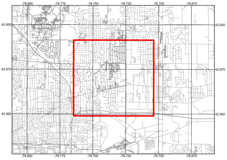
Figure 3: Area boundary

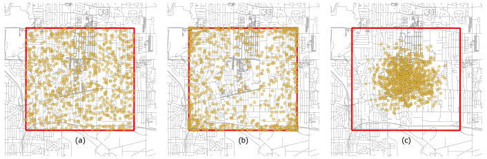
Figure 4: Geographical distribution of students

Overall, by deliberately manipulating these three factors — geographic distribution, student population, and average ridership- we were able to create diverse and representative sets of synthetic students for the simulation. This approach provided us with valuable insights into the dynamics of student transportation and its associated challenges under various scenarios. Table 1 shows the 12 experimental settings.

Set	Students ($n$)	Ridership ($\bar{\rho}$)	Geography
1	400	0.3	$\alpha=1.00\quad\beta=1.00$
2	400	0.8	$\alpha=1.00\quad\beta=1.00$
3	800	0.3	$\alpha=1.00\quad\beta=1.00$
4	800	0.8	$\alpha=1.00\quad\beta=1.00$
5	400	0.3	$\alpha=0.45\quad\beta=0.45$
6	400	0.8	$\alpha=0.45\quad\beta=0.45$
7	800	0.3	$\alpha=0.45\quad\beta=0.45$
8	800	0.8	$\alpha=0.45\quad\beta=0.45$
9	400	0.3	$\alpha=6.50\quad\beta=6.50$
10	400	0.8	$\alpha=6.50\quad\beta=6.50$
11	800	0.3	$\alpha=6.50\quad\beta=6.50$
12	800	0.8	$\alpha=6.50\quad\beta=6.50$

Table 1: Experiment setting

The risk of implementing the open offer policy is represented by $P\left(\mathscr{K}\middle|\tau\right)$, the conditional probability that the savings, if any, due to fleet reduction do not compensate the cost of incentives for students given a certain incentive $\tau$. We do not know the exact relation between the incentive $\tau$ and the overall opt-out rate $\bar{r}$; though, one can conjecture that they are positively correlated. Then, we want to study the risk conditional to the incentive and the overall opt-out rate $P\left(\mathscr{K}\middle|\tau,\bar{r}\right)$. To do so, we simulate 500 replicates for each one of the 12 sets described in Table 1. The result for each set is shown in Figure 5, where the red area represents the combinations for $\tau$ and $\bar{r}$ that yielded in losses for the school district, i.e., the open policy failed. The color green indicates where the combinations for $\tau$ and $\bar{r}$ yielded gains or overall savings for the school district.

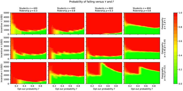
Figure 5: Contour plot for $P\left(\mathscr{K}\middle|\tau,\bar{r}\right)$ for each data set

We have identified notable variations in risk levels among the different sets. The instance with the highest risk among these sets is set number 3. A larger number of students, a lower average ridership, and a uniform spatial distribution characterize this particular set. The combination of these factors poses a higher risk regarding student transportation dynamics. With more students and lower ridership, the transportation system may need help in efficiently accommodating the transportation needs of the students. Additionally, it appears that the uniform spatial distribution adds complexity as students are spread out across the area, potentially leading to longer travel distances and increased transportation time.

On the other hand, the set with the lowest risk is set number 11. This set exhibits a similar student population size and average ridership as other sets, but the key difference lies in the spatial distribution of students. In set number 11, students are more concentrated around the school. This concentrated spatial distribution potentially reduces the overall travel distances and may promote shorter travel times for students. As a result, the transportation system in this scenario is more efficient and less prone to potential disruptions or delays.

To aggregate the risk into one metric per data set, let us define

$$P_{\bar{\tau}}\left(\mathscr{K}\right)=\sum_{\tau}^{\bar{\tau}}\sum_{\bar{r}}P\left(\mathscr{K}\middle|\tau,\bar{r}\right)p(\bar{r})p(\tau)$$ (56)

to represent the overall mean of the risk for each data set. For computing this metric, we assume the possible values for $\tau$ are uniformly distributed between 0 and $\bar{\tau}$ US dollars, and $\bar{r}$ ranges uniformly between 0 and 1.

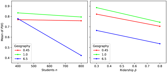
Figure 6: Interaction plot of $P_{\bar{\tau}}\left(\mathscr{K}\right)$ for $\bar{\tau}=5,000$ US dollars.

Based on the analysis of the instances described in Table 1 and the corresponding mean values of aggregated risk displayed in Figure 6, it can be tentatively concluded that there is a notable reduction in risk when students are concentrated around the school, particularly in the context of implementing the open offer policy. This finding holds particular promise for schools with larger student populations and higher ridership.

When students are more concentrated around the school, the number of students requiring long trips decreases, resulting in routes with fewer students. This concentration is especially advantageous in schools with a larger student population, as a significant number of students living far from the school are more likely to opt-out of transportation services. Consequently, the need for underutilized routes is reduced.

5.2 Case study: the Williamsville Central School District

The Williamsville Central School District (WCSD) is an esteemed public school district situated in Williamsville, New York, in the United States. The WCSD serves the suburban communities of Williamsville, Amherst, and Clarence in Erie County, comprising a total of 13 schools in the district. It includes six Elementary Schools (ELs), four Middle Schools (MIs), and three High Schools (HIs). The ELs are strategically located throughout the district, providing education from kindergarten through fifth grade. The MIs cater to students in grades six through eight, while the HIs are dedicated to students in grades nine through twelve.

Encompassing an area of approximately 40 square miles, WCSD accommodates over 10,000 students, nurturing their academic growth and development. The district strongly emphasizes student transportation, recognizing the importance of safe and efficient travel. To facilitate this, WCSD operates a fleet of nearly 100 buses, maintaining a ratio of approximately 2:3 between their own buses and those provided by a contractor. This robust transportation system ensures that students can access the various schools within the district effectively.

The dispersion of students and their corresponding schools was visually represented in Figure 7 following a normalization process. This process involved calculating the distances between the students and a common reference point, enabling a fair comparison across all schools. The positions of the students were then adjusted based on this normalization. To quantify the dispersion level, the standard deviation of the student’s positions relative to the center of mass was computed. This measure provided a comprehensive assessment of the student’s spread out within each school, indicating the degree of dispersion.

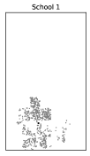
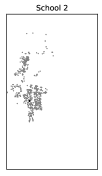
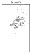
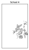
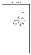
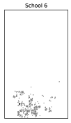
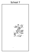
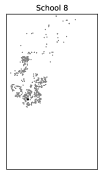
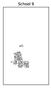
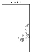
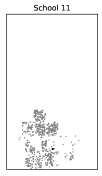
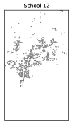
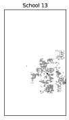
Figure 7: Dispersion fo students for the schools in the WCSD in 2014 - 2015

Upon analyzing the data, it was observed that the level of dispersion varied among the schools, as shown in Table 2. School 9 exhibited the lowest level of dispersion, with a value of 0.33. This indicates that the students in school 9 were relatively closer to each other and formed a more compact cluster. On the other hand, school 8 displayed the highest level of dispersion among all the schools, with a value of 0.54. This suggests that the students in school 8 were more widely distributed, with larger distances between individual students and the center of mass.

Table 2 also shows the values for the ridership. These values were obtained through a comprehensive data collection effort to estimate the likelihood of students not appearing at their assigned bus stops. The data collection process involved meticulous recording of student headcounts on each bus during morning and afternoon periods. The analysis revealed that the probability of a student not showing up at their designated bus stop was inconsistent across all schools. Instead, it exhibited significant variations depending on the specific educational institution, ranging from 22% to 72%. This finding underscores the importance of considering individual school dynamics and factors that may impact student attendance rates.

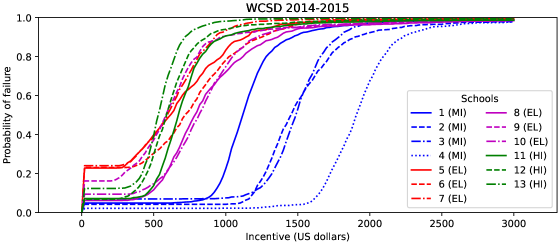
Figure 8: Probability of failure as function of the incentive

Figure 8 depicts the relationship between the probability of failure and the incentive per student. As expected, the likelihood of failure increases with higher incentives. However, there are significant variations in behavior among different schools. Middle schools exhibit a slower growth rate compared to High schools and Elementary schools, suggesting their ability to offer larger incentives while maintaining a low probability of failure. On the other hand, Elementary schools such as schools 5 and 7 experience probabilities of failure exceeding 0.2 even with minimal incentives.

A common characteristic across all curves is the rapid increase in the probability of failure once the incentive surpasses a certain threshold, resembling the probability function of a logistic regression. Based on its unique characteristics, this implies that each school has a point at which implementing the Open Offer Policy becomes unfeasible due to the associated risk.

Finally, Table 2 presents the aggregate risk defined in equation (56) for various maximum incentive levels, denoted as $\bar{\tau}$. Cases where the aggregate risk is below 10% are highlighted. As previously mentioned, Middle schools (MI) perform well, achieving a low risk even with relatively high incentives. Among Middle schools, the one with the lowest level of dispersion demonstrates the best performance, consistent with the findings from Section 5.1.

					Aggregate risk $P_{\bar{\tau}}(\mathcal{K})$
School	group	dispersion	ridership	students	$\bar{\tau}=300$	$\bar{\tau}=500$	$\bar{\tau}=1000$	$\bar{\tau}=2000$	$\bar{\tau}=3000$
1	MI	0.43	53%	1219	0.046	0.047	0.062	0.439	0.620
2	MI	0.48	52%	647	0.039	0.040	0.041	0.278	0.505
3	MI	0.45	62%	676	0.065	0.067	0.069	0.295	0.526
4	MI	0.39	69%	984	0.020	0.021	0.021	0.089	0.366
5	EL	0.50	69%	956	0.215	0.256	0.442	0.696	0.794
6	EL	0.48	72%	467	0.217	0.233	0.385	0.660	0.771
7	EL	0.37	72%	517	0.226	0.262	0.481	0.730	0.818
8	EL	0.54	67%	655	0.059	0.068	0.254	0.578	0.710
9	EL	0.33	62%	660	0.158	0.207	0.458	0.701	0.793
10	EL	0.47	64%	842	0.088	0.099	0.263	0.594	0.722
11	HI	0.43	28%	863	0.067	0.077	0.346	0.649	0.760
12	HI	0.48	36%	544	0.065	0.103	0.421	0.694	0.792
13	HI	0.40	22%	712	0.117	0.157	0.499	0.744	0.828

Table 2: Data and aggregated risk for the schools in the WCSD in 2014-2015

6 Discussion and Future Research

In this paper, we introduce a new variant of the School Bus Routing Problem called School Bus Routing Problem with Open Offer Policy (SBRP-OOP), which focuses on finding a pricing strategy that balances incentive payments for students who choose not to use the bus with the savings achieved by operating fewer buses. By excluding students who accept the incentive from the routing process, SBRP-OOP aims to address multiple objectives simultaneously for a single school. This involves selecting the optimal set of stops from a pool of potential stops, assigning students to stops while considering factors like maximum walking distance and student capacity, and generating routes that minimize bus travel distance.

To evaluate the effectiveness of SBRP-OOP, we conducted simulations using both synthetic and real data. Our initial analysis suggests that when students concentrates around the school the risk associated with implementing the Open Offer Policy in student transportation is reduced, especially for schools with larger student populations and higher ridership.

When considering real instances, we found that the Open Offer Policy can be implemented with low risk and promising benefits in certain schools, particularly Middle schools. However, for some Elementary schools, implementing the policy seems impractical. Additionally, among the schools that benefit from the Open Offer Policy, those with a more compact distribution of students around the school experience greater gains.

While these observations indicate potential benefits and risk reduction associated with concentrating students around the school, it is important to approach these conclusions cautiously. Other factors such as local infrastructure, geographical constraints, and specific school transportation policies may influence the outcomes. Therefore, further research and analysis are necessary to validate and explore these findings in diverse contexts.

References

- Bertsimas et al. [2020] Dimitris Bertsimas, Arthur Delarue, William Eger, John Hanlon, and Sebastien Martin. Bus routing optimization helps boston public schools design better policies. Interfaces, 50:37–49, 1 2020. ISSN 1526551X. doi: 10.1287/inte.2019.1015.
- Bodin and Berman [1979] Lawrence D Bodin and Lon Berman. Routing and scheduling of school buses by computer. Transportation Science, 13(2):113–129, 1979.
- Bowerman et al. [1995] Robert Bowerman, Brent Hall, and Paul Calamai. A multi-objective optimization approach to urban school bus routing: Formulation and solution method. Transportation Research Part A: Policy and Practice, 29(2):107–123, 1995.
- Braca et al. [1997] Jeffrey Braca, Julien Bramel, Bruce Posner, and David Simchi-Levi. A computerized approach to the new york city school bus routing problem. IIE Transactions, 29(8):693–702, 1997.
- Caceres et al. [2017] Hernan Caceres, Rajan Batta, and Qing He. School bus routing with stochastic demand and duration constraints. Transportation Science, 51(4):1349–1364, 2017. doi: 10.1287/trsc.2016.0721.
- Calvete et al. [2020] Herminia I Calvete, Carmen Galé, José A Iranzo, and Paolo Toth. A partial allocation local search matheuristic for solving the school bus routing problem with bus stop selection. Mathematics, 8(8):1214, 2020.
- Calvete et al. [2021] Herminia I Calvete, Carmen Galé, José A Iranzo, and Paolo Toth. The school bus routing problem with student choice: a bilevel approach and a simple and effective metaheuristic. International Transactions in Operational Research, 2021.
- Chapleau et al. [1985] Luc Chapleau, Jacques-A Ferland, and Jean-Marc Rousseau. Clustering for routing in densely populated areas. European Journal of Operational Research, 20(1):48–57, 1985.
- Desmond [2022] Mike Desmond. Shortage of bus drivers hurts buffalo public school’s academic recovery from covid-19, 2022. URL https://www.wbfo.org/education/2022-09-21/shortage-of-bus-drivers-hurts-buffalo-public-schools-academic-recovery-from-covid-19.
- Dulac et al. [1980] Gilles Dulac, Jacques A Ferland, and Pierre A Forgues. School bus routes generator in urban surroundings. Computers & Operations Research, 7(3):199–213, 1980.
- Ellegood et al. [2019] William A. Ellegood, Stanislaus Solomon, Jeremy North, and James F. Campbell. School bus routing problem: Contemporary trends and research directions. Omega, page 102056, 2019. ISSN 0305-0483. doi: https://doi.org/10.1016/j.omega.2019.03.014. URL http://www.sciencedirect.com/science/article/pii/S0305048318305127.
- Farzadnia and Lysgaard [2021] Farnaz Farzadnia and Jens Lysgaard. Solving the service-oriented single-route school bus routing problem: Exact and heuristic solutions. EURO Journal on Transportation and Logistics, 10:100054, 2021.
- Kinable et al. [2014] Joris Kinable, Frits CR Spieksma, and Greet Vanden Berghe. School bus routing—a column generation approach. International Transactions in Operational Research, 21(3):453–478, 2014.
- Lando [2023] Lia Lando. Parents in buffalo continue to advocate for staggered start times to deal with bus driver shortage, 2023. URL https://www.wkbw.com/news/local-news/parents-in-buffalo-continue-to-advocate-for-staggered-start-times-to-deal-with-bus-driver-shortage.
- Li and Chow [2021] Mengyun Li and Joseph YJ Chow. School bus routing problem with a mixed ride, mixed load, and heterogeneous fleet. Transportation Research Record, 2675(7):467–479, 2021.
- Newton and Thomas [1969] Rita M Newton and Warren H Thomas. Design of school bus routes by computer. Socio-Economic Planning Sciences, 3(1):75–85, 1969.
- Park and Kim [2010] Junhyuk Park and Byung-In Kim. The school bus routing problem: A review. European Journal of Operational Research, 202(2):311–319, 2010.
- Parvasi et al. [2017] Seyed Parsa Parvasi, Mehdi Mahmoodjanloo, and Mostafa Setak. A bi-level school bus routing problem with bus stops selection and possibility of demand outsourcing. Applied Soft Computing, 61:222 – 238, 2017. ISSN 1568-4946. doi: https://doi.org/10.1016/j.asoc.2017.08.018.
- Riera-Ledesma and Salazar-González [2012] Jorge Riera-Ledesma and Juan-José Salazar-González. Solving school bus routing using the multiple vehicle traveling purchaser problem: A branch-and-cut approach. Computers & Operations Research, 39(2):391–404, 2012.
- Riera-Ledesma and Salazar-González [2013] Jorge Riera-Ledesma and Juan José Salazar-González. A column generation approach for a school bus routing problem with resource constraints. Computers & Operations Research, 40(2):566–583, 2013.
- Salhi and Rand [1989] Said Salhi and Graham K Rand. The effect of ignoring routes when locating depots. European journal of operational research, 39(2):150–156, 1989.
- Schittekat et al. [2013] Patrick Schittekat, Joris Kinable, Kenneth Sörensen, Marc Sevaux, Frits Spieksma, and Johan Springael. A metaheuristic for the school bus routing problem with bus stop selection. European Journal of Operational Research, 229(2):518–528, 2013.