Far-from-equilibrium criticality in the Random Field Ising Model with Eshelby Interactions

Abstract

We study a quasi-statically driven random field Ising model (RFIM) at zero temperature with interactions mediated by the long-range anisotropic Eshelby kernel. Analogously to amorphous solids at their yielding transition, and differently from ferromagnetic and dipolar RFIMs, the model shows a discontinuous magnetization jump associated with the appearance of a band-like structure for weak disorder and a continuous magnetization growth, yet punctuated by avalanches, for strong disorder. Through a finite-size scaling analysis in 2 and 3 dimensions we find that the two regimes are separated by a finite-disorder critical point which we characterize. We discuss similarities and differences between the present model and models of sheared amorphous solids.

A large variety of phenomena on very different scales involve abrupt collective responses to an applied force or field, known as avalanches. Qualitative similarities and observed scale invariance in the distribution of these avalanches have prompted the development of simple models whose relevance to actual physical situations has been argued within the framework of universality and renormalization group Fisher (1998); Sethna et al. (2001); Alava et al. (2006); Dahmen and Ben-Zion (2011); Sethna et al. (2017); Perez-Reche (2017); Wiese (2022). The systems of interest involve quenched disorder in one form or another, interactions between a large number of degrees of freedom, and evolve far from equilibrium. As thermal fluctuations are generally suppressed and driving rates very slow, a first conceptual simplification is to consider the limit of a quasi-static driving at zero temperature.

Scale invariance in such athermal quasi-statically (AQS) driven disordered systems can still appear in quite diverse contexts, which one can sort out according to the required number of fine-tuned control parameters. No fine-tuning at all is needed in the case of self-organized criticality Bak et al. (1987, 1988) and marginal stability Müller and Wyart (2015). Fine-tuning the magnitude of the driving force corresponds to the broad class of depinning critical transitions, as in elastic manifolds in a random environment Thomas Nattermann et al. (1992); Fisher (1998); Wiese (2022). Finally, by tuning an additional parameter, the strength of the disorder, one may have a critical point separating a regime with a discontinuous, “snapping”, response associated with an extensive avalanche from a regime with an essentially continuous, “popping”, response punctuated by finite avalanches Sethna et al. (2001). The archetype of such a disorder-controlled criticality is provided by the AQS driven random-field Ising model (RFIM) Sethna et al. (1993) which is used to describe hysteresis and “crackling noise” across a variety of systems Sethna et al. (2001, 2006). We focus here on this third type of scale invariance and on the associated universality classes. It is well known that the dimension of space and the characteristics of the order parameter are main factors determining the universality class. Our aim is to understand the role played by nature of the interactions. Note that symmetries such as time-reversal and internal symmetries are expected to be less important in these far-from-equilibrium critical points because they are anyhow broken by the AQS dynamics.

A broad and important class of AQS driven disordered systems is represented by sheared amorphous solids. When an amorphous material such as glass is uniformly deformed from an initial quiescent state, one may observe two different types of yielding behavior: brittle yielding, where the sample abruptly breaks with a strong strain localization in the form of a system-spanning shear band, and ductile yielding, in which the sample gradually deforms and flows with the presence of subextensive avalanches. The nature of the yielding transition depends on the stability and the degree of structural and mechanical disorder of the material, which can somewhat be varied through the preparation protocol such as the cooling rate for a glass Rodney et al. (2011); Kumar et al. (2013); Vasoya et al. (2016); Fan et al. (2017); Ozawa et al. (2018). Poorly-annealed samples, which have a lower stability and a higher degree of disorder, show ductile yielding, while well-annealed samples with a higher stability and less disorder display brittle yielding. It has been argued that the two types of yielding behavior are separated by a disorder (or stability) controlled critical point akin to that of an AQS driven RFIM Ozawa et al. (2018, 2020). Although debated Barlow et al. (2020); Richard et al. (2021); Pollard and Fielding (2022), this proposal has recently received strong support from our extensive numerical study of a uniformly sheared mesoscopic elasto-plastic model Rossi et al. (2022). The similarity between the transition pattern in the RFIM and in mesoscopic models of uniformly sheared amorphous solids has been established at the mean-field level Ozawa et al. (2018); Rossi and Tarjus (2022); Borja da Rocha and Truskinovsky (2020), but in finite dimensions the geometry and the spatial structure of the large avalanches are clearly different in sheared glasses and in the conventional RFIM. One major ingredient that is missing in the standard RFIM model is the anisotropy and long-range nature of the elastic interaction (couplings are instead short-range, isotropic and all negative). Therefore, in order to mimic the quadrupolar plastic events observed in deformed amorphous materials and their interactions leading to the appearance of shear bands we replace the nearest-neighbor ferromagnetic interactions of the RFIM by the Eshelby propagator of linear elasticity Eshelby (1957); Picard et al. (2004). This leads to an Eshelby-RFIM with anisotropic long-ranged couplings:

$$\mathcal{H}(\{s_{i}\})=-\frac{1}{2}\sum_{i,j}G_{ij}s_{i}s_{j}-\sum_{i}(h_{i}+H)s_{i},$$ (1)

where the Ising spin variables $s_{i}=\pm 1$ are placed at the vertices of a $d$-dimensional cubic lattice, $h_{i}$ is the local random field, independently chosen from a normal distribution of zero mean and variance $R^{2}$, $H$ is the applied magnetic field, and $G_{ij}\equiv G({\bf r}_{ij})$ is the Eshelby kernel, which decays with distance as $r_{ij}^{-d}$ and has the angular dependence of a quadrupole-quadrupole interaction, e.g., in $2d$, $G({\bf r}_{ij})=\cos(4\theta_{ij})/(\pi r_{ij}^{2})$, where $\theta_{ij}$ is the angle relative to the $x$-axis. This kernel explicitly breaks isotropy (beyond mere lattice effects), the $x$-axis playing the role of the direction of shear. To avoid spin self-interaction we moreover fix $G_{ii}=0$. More details on the interaction kernel are given in the Supplemental Material (SM).

Our goal is then two-fold: first, to investigate the issue of universality classes for disorder-controlled criticality in AQS driven disordered systems and, second, to explore the possibility of building an effective theory for the yielding transition of uniformly sheared amorphous solids. In this respect, the description provided by elasto-plastic models (EPMs) Picard et al. (2004); Nicolas et al. (2018) falls short because although a drastic phenomenological simplification of the real processes at play, it is still too complex to be analyzed with accurate and controlled theoretical methods. In order to achieve our goal, we perform extensive numerical simulations of the Eshelby-RFIM in two and three dimensions, and we compare the results to their counterparts obtained for EPMs. (Direct numerical simulations of atomistic models are limited to sizes which do not allow a thorough finite-size scaling analysis.)

We follow the AQS dynamics of the model starting from a stable initial condition with all spins pointing down at a large negative field $H=-50$. The field is then increased (we study the ascending branch of the hysteresis loop) until a first spin becomes unstable. A spin $s_{i}$ becomes unstable when its effective local field $h_{i}^{\rm eff}=\sum_{j\neq i}G_{ij}s_{j}+h_{i}+H$ becomes such that $h_{i}^{\rm eff}s_{i}<0$. This may then lead other spins to become unstable, thereby leading to a collective avalanche which stops when all spins are stable again. Note that since the interaction kernel is not positive definite the dynamics is no longer Abelian and the order in which the spins are flipped in an avalanche may change the precise outcome Magni (1999); Kurbah and Shukla (2011); Nampoothiri et al. (2017). In the present work we choose an update in which at each step we pick at random one of the unstable spins to flip it and we recalculate the stability of all other spins (see the SM). To properly average over the random-field disorder and perform finite-size scaling analyses when necessary, we consider systems of linear size $L=N^{1/d}$ from $256$ to $2048$ in $d=2$ and $48$ to $128$ in $d=3$ with $200$-$3000$ samples for each size and we use periodic boundary conditions.

Our first result is to show that changing the nature of the interaction to an Eshelby kernel indeed drastically modifies the geometry and the spatial structure of the large avalanches. We illustrate the transition pattern as a function of the disorder strength $R$ by plotting the volume-averaged magnetization $m=(1/N)\sum_{i=1}^{N}s_{i}$ versus $H$ and some spin configurations at selected values of $H$ for a few typical $3d$ samples in Fig. 1(a). For a large $R$ the evolution is rather smooth and the avalanches are subextensive and uniformly distributed in space. On the other hand for a small $R$, the magnetization displays a jump of O(1) at a specific “coercive field” $H_{\rm co}$ that is followed by an apparently linear regime. In both cases the magnetization saturates at $+1$ for a large enough positive applied field. The striking feature when comparing to the behavior of the convential RFIM Sethna et al. (1993, 2001, 2006) is that the jump is associated with a system-spanning avalanche that is spatially localized in a band (see the inset). This is reminiscent of the shear band found in the brittle yielding of sheared amorphous solids. The similarity can be made even more vivid by looking at the cumulative plastic strain in the AQS evolution of an elasto-plastic model (EPM), which is the accumulated plastic activity $\gamma_{i}^{\rm pl}$ at each site $i$ averaged over the whole lattice. In Fig. 1(b) we plot the results for the $3d$ model that we have studied in Ref. [Rossi et al., 2022] for two values of the initial disorder corresponding to ductile and brittle yielding. The correspondence between the two models is that a down spin represents a site that has not yielded and an up spin a site that has had a plastic event. Note that the presence of a magnetization jump corresponding to a single band of flipped spins is not found in the previously studied RFIM models, including those with long-range dipole-dipole interactions Sethna et al. ; Magni (1999); Dubey et al. (2015), where one observes either a relatively isotropic macroscopic avalanche Sethna et al. ; Sethna et al. (2001); Pérez-Reche and Vives (2003, 2004) or exotic labyrinthine patterns Magni (1999); Dubey et al. (2015). This suggests that the Eshelby kernel with its specific quadrupolar symmetry is the key ingredient for reproducing the strong band-like behavior .

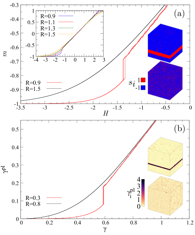
Figure 1: (a): Magnetization $m$ versus applied field $H$ in the $3d$ Eshelby-RFIM for $R=1.5$ (black) and $R=0.9$ (red) (3 independent samples with $L=128$). Upper left inset: $m(H)$ over a larger range of $H$ up to $m=+1$ (here $L=104$). Lower right inset: Spin configurations at $H=-1.2$ for $R=0.9$ (top) and $R=1.5$ (bottom). (b): Cumulative volume-averaged plastic strain $\gamma^{\rm pl}$ versus imposed strain $\gamma$ for the $3d$ uniformly sheared EPM studied in Ref. [Rossi et al., 2022] and two values of the initial disorder $R$, $R=0.3$ (brittle) and $R=0.8$ (ductile). Inset: Real-space configurations of the local plastic activity $\gamma_{i}^{\rm pl}$ at $\gamma=0.7$ for $R=0.3$ (top) and $R=0.8$ (bottom).

We now consider the discontinuous regime at small disorder and the mechanism of band formation. The magnetization can be taken as an order parameter but we find it more convenient to also introduce an alternative order parameter which better captures the appearance of a band. In each sample we monitor $m_{\rm b}$, the maximum of all the line-averaged magnetizations in $2d$ and plane-averaged magnetizations in $3d$, where lines/planes are perpendicular to the axes: $m_{\rm b}=-1$ at the beginning of the process and it abruptly jumps to a value close to $+1$ at the sample-dependent coercive field $H_{\rm co}$. Averaging over disorder, i.e., samples, which we indicate by an overline, rounds the discontinuity, but a finite-size scaling of the associated susceptibilities shows that they diverge with $L$ at a well-defined coercive field (see the SM), so that the discontinuity persists in the thermodynamic limit.

A major difference between the Eshelby RFIM and the EPMs is the possibility for a site to undergo many repeated events: a spin essentially flips once over the whole evolution of the system (see the SM) whereas a site in a uniformly sheared EPM can yield a large number of times. This is particularly important in the process of band formation. To contrast the behavior of the two types of models we compute the band profile along the direction $x_{\perp}$ perpendicular to band propagation right at the coercive field. The band profile for the Eshelby-RFIM is given by $\rho_{\rm band}^{\rm RFIM}(L,x_{\perp})=(1/L^{d-1})\sum_{\mathbf{x}_{\parallel}}s_{(\mathbf{x}_{\parallel},x_{\perp})}$ and that for the EPM by $\rho_{\rm band}^{\rm EPM}(L,x_{\perp})=(1/L^{d-1})\sum_{\mathbf{x}_{\parallel}}\gamma^{\rm pl}_{(\mathbf{x}_{\parallel},x_{\perp})}$, where $(\mathbf{x}_{\parallel},x_{\perp})\equiv i$ specify the location of a site and we have shifted $x_{\perp}$ in each sample such that $x_{\perp}=0$ corresponds to the center of the band. In the RFIM, a jump of O(1) in the magnetization implies that the associated band volume scales as $N=L^{d}$. As $\overline{\rho_{\rm band}^{\rm RFIM}}(L,x_{\perp}=0)$ should be essentially independent of $L$, one then expects that the band width scales as $L^{v}$ with $v=1$, so that the change of magnetization summed over the whole band goes as $L^{d}$. This is verified by the finite-size scaling result illustrated in Fig. 2(a) for the $3d$ case. On the other hand, the number of plastic events per site in the shear band of the EPM appears to grow with the system size. This translates into $\overline{\rho_{\rm band}^{\rm EPM}}(L,x_{\perp}\approx 0)\sim L^{u}$ with $u>0$ while, concomitantly, the width of the shear band scales as $L^{v}$ with $v=1-u<1$. This leads to a difference between the scaling of the number of sites and of plastic events: the total number of sites in the shear band goes as $L^{d-1+v}$ while the total number of plastic events in the shear band goes as $N=L^{d}$. We find that $v\approx 0.68$ and $u\approx 0.32$ for the $3d$ EPM: see Fig. 2(b). In the SM we also provide additional evidence of the difference between Eshelby-RFIM and EPM in the weak-disorder, discontinuous regime by looking at the avalanche distribution and the marginal stability property.

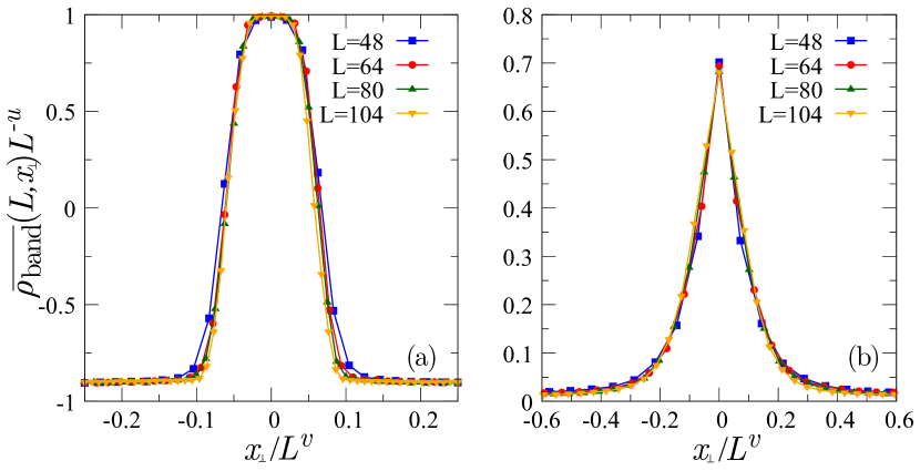
Figure 2: Scaling plot of the average band profiles $\overline{\rho_{\rm band}}(L,x_{\perp})/L^{u}$ versus $x_{\perp}/L^{v}$ for the $3d$ Eshelby-RFIM (a) and $3d$ EPM (b) right at the discontinuous transition, obtained for $R=0.9$ and $R=0.25$, respectively. The collapses are obtained for $u=0$ and $v=1$ for the Eshelby-RFIM, and $u=0.32$ and $v=0.68$ for the EPM.

Between the discontinuous regime at small $R$ and the crossover one at large $R$ one expects a disorder-controlled critical point. To pinpoint the latter and characterize its properties we have performed a finite-size scaling analysis. Inspired by our previous EPM work Rossi et al. (2022) we have introduced two different order parameters, the maximum jump of the magnetization, $\Delta m_{\rm max}$, and that of the quantity $m_{\rm b}(H)$ (see above), $\Delta m_{\rm b,max}$, where the maximum is taken for each sample over a whole AQS evolution from $H=-50$ to a very large $H$ (until all spins become positive). By construction, both are nonzero of O(1) when the sample displays a strong band-like avalanche with a discontinuous magnetization jump, whereas they are nearly $0$ for a gradual evolution of the magnetization curve. As an illustration we display in Fig. 3 the disorder-averaged value $\overline{\Delta m_{\rm b,max}}(R,L)$ and the associated disconnected susceptibility $\chi_{\rm dis,b}^{\rm OP}(R,L)=L^{d-1}{\rm Var}(\Delta m_{\rm b,max})$, where Var denotes the variance, in $2d$ and $3d$. The behavior observed as a function of the linear system size $L$ is typical of what is expected for a critical point at a value $R_{c}(L)$ corresponding to the position of the susceptibility peak. Similar curves (but with more noise) are obtained for $\overline{\Delta m_{\rm max}}(R,L)$ and the associated disconnected susceptibility $\chi_{\rm dis}^{\rm OP}(R,L)=L^{d}{\rm Var}(\Delta m_{\rm max})$. We analyze the results through a finite-size scaling ansatz in which we assume that, despite the anisotropy of the interactions, criticality is characterized by a unique diverging correlation length with exponent $\nu$ :

$$\overline{\Delta m_{\rm max}}\sim L^{-\frac{\beta}{\nu}}\mathcal{M}(rL^{\frac{1}{\nu}}),\,\overline{\Delta m_{\rm b,max}}\sim L^{-\frac{\beta_{\rm b}}{\nu}}\mathcal{M}_{\rm b}(rL^{\frac{1}{\nu}}),$$ (2)

$$\chi_{\rm dis}^{\rm OP}(R,L)\sim L^{\frac{\bar{\gamma}}{\nu}}\,\bar{\Psi}(rL^{\frac{1}{\nu}}),\,\chi_{\rm dis,b}^{\rm OP}(R,L)\sim L^{\frac{\bar{\gamma}_{\rm b}}{\nu}}\,\bar{\Psi}_{\rm b}(rL^{\frac{1}{\nu}}),$$

where $r=(R-R_{c}(L))/R$ is the relative distance from the critical disorder, $\beta$, $\beta_{\rm b}$, $\bar{\gamma}$, $\bar{\gamma}_{\rm b}$ are critical exponents, and $\mathcal{M}$, $\bar{\Psi}$, $\mathcal{M}_{\rm b}$, $\bar{\Psi}_{\rm b}$ are scaling functions. Note that by construction, $\bar{\gamma}/\nu\leq d$, $\bar{\gamma}_{\rm b}/\nu\leq d-1$ and, for consistency, $\beta/\nu,\,\beta_{\rm b}/\nu\geq 0$.

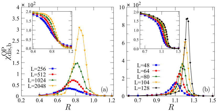
Figure 3: Disconnected susceptibility $\chi^{\rm OP}_{\rm dis,b}(R,L)$ and associated disorder-averaged order parameter $\overline{\Delta m_{\rm b,max}}$ (insets) versus disorder strength $R$ for several linear system sizes $L$ for the $2d$ (a) and the $3d$ (b) Eshelby-RFIM.

We have used four different methods to determine the critical exponents and functions: i) power-law fits to the maximum and the width of the susceptibilities, ii) power-law fit to the drift of the critical disorder, $R_{c}(\infty)-R_{c}(L)\sim L^{-1/\nu}$, iii) empirical scaling collapses of the data according to Eq. (LABEL:eq:FSS) by adjusting the exponents, and iv) a fit to a (flexible) analytical form for the susceptibility master-curves Shekhawat et al. (2013). We have also checked that compatible (but not as good) results for the exponents are obtained by looking at the disconnected susceptibilities defined from $m(H)$ and $m_{\rm b}(H)$ (instead of $\Delta m_{\rm max}$ and $\Delta m_{\rm b,max}$) when evaluated at their maximum over $H$ and at the critical disorder $R_{c}(L)$. On the other hand, the connected susceptibilities which must be obtained as numerical derivatives with respect to $H$ cannot be reliably computed and in any case vary much less with $L$ than the disconnected ones. Details are provided in the SM. In Fig. 4 we illustrate the outcome with a collapse of the disconnected susceptibilities and the corresponding average order parameters (insets) for the $3d$ case. We find for the $3d$ Eshelby-RFIM

$$\bar{\gamma}/\nu\approx 1.65-1.75,\;\beta/\nu\approx 0.58-0.66,\;\nu\approx 1.2-2.4,$$ (3)

$$\bar{\gamma}_{\rm b}/\nu\approx 1.77-1.9,\;\beta_{\rm b}/\nu\approx 0.04-0.12,$$

where the rather large error bars include the different methods of determination mentioned above. (We note that the procedures are less sensitive to the value of $1/\nu$ than to that of the other exponents, so that $\nu$ is more poorly determined.) The exponents satisfy the bounds given above and one can also push further the scaling ansatz to relate them. Indeed, at criticality one expects that the spatial correlations of the sample-to-sample spin fluctuations become scale-free with a power-law exponent related to that of the divergence of the disconnected susceptibility $\chi_{\rm dis}^{\rm OP}$. If one assumes that the anisotropy manifests itself in the prefactor but not in the power-law dependence, this exponent is simply $d-\bar{\gamma}/\nu$ (an integral over the volume then gives back the divergence of $\chi_{\rm dis}^{\rm OP}$). The scaling dimension of the average order parameter at the critical point is then $-(d-\bar{\gamma}/\nu)/2$. A similar reasoning holds for the quantities defined from $\Delta m_{\rm b,max}$, except that the relevant correlation function is now for spins within a line (in $2d$) or a plane (in $3d$) associated with the incipient critical band. This new correlation function is expected to decay as a power law at large distance with exponent $d-1-\bar{\gamma}_{\rm b}/\nu$ (an integral over the line or the plane then gives back the divergence of $\chi_{\rm dis,b}^{\rm OP}$), so that the average order parameter should scale with system size with an exponent $-(d-1-\bar{\gamma}_{\rm b}/\nu)/2$. Putting this together leads to $2\beta/\nu=d-\bar{\gamma}/\nu$ and $2\beta_{\rm b}/\nu=d-1-\bar{\gamma}_{\rm b}/\nu$, which is verified within error bars by the values in Eq. (LABEL:eq:3Dexponents). These results provide a strong support for the presence of a critical point at a finite value of the disorder strength in $3d$. Note that the values in Eq. (LABEL:eq:3Dexponents) seem to indicate that $\bar{\gamma}/\nu\approx\bar{\gamma}_{\rm b}/\nu$ and $\beta/\nu\approx\beta_{\rm b}/\nu+(1/2)$, but we have not been able to find strong arguments to support this finding beyond invoking Occam’s razor.

The situation in $2d$ is more problematic as we find that $\bar{\gamma}_{\rm b}/\nu\approx 1.00-1.05$ (but being larger than $1$ is forbidden by the bound) and $\beta_{\rm b}/\nu\approx-0.04-0.00$ (but being negative is not physical). Correspondingly, we roughly estimate that $\bar{\gamma}/\nu\approx 1.05-1.25$, $\beta/\nu\approx 0.45-0.48$, and $\nu\approx 2.3-3.0$ (see the SM). The model does not seem to be at its lower critical dimension because, contrary to what would then be expected, the critical disorder $R_{c}(L)$ slowly increases with $L$ (see Fig. 3) instead of decreasing as, e.g., found in the standard AQS driven RFIM in $d=2$ Spasojević et al. (2011); Hayden et al. (2019). This points to a discontinuous transition for $m_{\rm b}$, i.e., the sudden emergence of a positively magnetized line at some $R_{c}$, but the band width itself appears to scale sub-linearly with $L$, like $L^{1-\beta/\nu}$. This corresponds to an unusual scenario in which the disorder-controlled transition between the discontinuous and the continuous regimes is a fluctuation-induced discontinuous one for the band-order parameter but a continuous one for the magnetization.

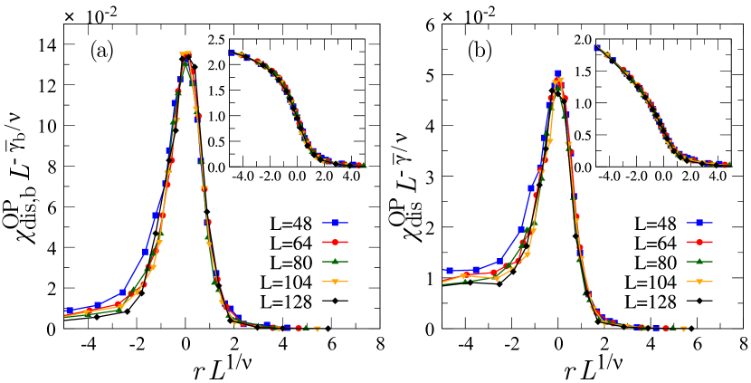
Figure 4: Finite-size scaling collapse of the disconnected susceptibilities $\chi^{\rm OP}_{\rm dis,b}(R,L)$ with $\bar{\gamma}_{\rm b}/\nu=1.81$ (a) and $\chi^{\rm OP}_{\rm dis}(R,L)$ with $\bar{\gamma}/\nu=1.7$ (b) in $3d$. Insets: Same for $\overline{\Delta m_{\rm b,max}}$ with $\beta_{\rm b}/\nu=0.08$ (a) and $\overline{\Delta m_{\rm max}}$ with $\beta/\nu=0.62$ (b). In all cases $\nu=1.4$. Compare with Eq. (LABEL:eq:FSS).

We can finally compare the critical behavior of the Eshely-RFIM just obtained with that of the EPM studied in Ref. [Rossi et al., 2022]. As already mentioned, we find that the qualitative features (transition pattern, shape of the large-scale avalanches, dominance of the sample-to-sample fluctuations) are very similar. We also observe that the critical exponents in the two models are close and evolve in the same direction between $3d$ and $2d$. The better-determined ratio $\bar{\gamma}_{\rm b}/\nu$ is about $10\%$ higher in the Eshelby-RFIM than in the EPM  but, considering the difficulty to reliably extract exponent values in out-of-equilibrium disordered systems Perkovic et al. (1996); *perkovic1999, this difference may not be significant enough for reaching a definite conclusion. Furthermore, the exponents $\bar{\gamma}/\nu$ and $\beta/\nu$ are compatible between the two models within error bars and, as displayed in Fig. S8 of the SM, the disconnected susceptibilities $\chi_{\rm dis}^{\rm OP}(R,L)$ in the $3d$ case, where they can be more reliably computed, all collapse very well onto the same master-curve. This suggests that the Eshelby-RFIM and the EPM are in the same universality class. However, even larger system sizes with then still more sophisticated scaling analyses (e.g., a detailed characterization of the system-spanning avalanches at criticality as in Refs. [Pérez-Reche and Vives, 2003, 2004] or of the spatial correlation functions) will be necessary to definitely settle the issue. On the other hand, we have shown ample evidence that the Eshelby-RFIM and the ferromagnetic RFIM clearly belong to distinct universality classes.

To sum up, we have introduced and numerically studied a version of the athermally and quasi-statically driven RFIM in which the interactions have the anisotropic and long-ranged form of the Eshelby propagator used in the theory of amorphous solids under deformation. We have found that the model shows a disorder-controlled transition between a discontinuous and a continuous regime, as the standard RFIM but with a different phenomenology that is instead very similar to that found in elasto-plastic models (EPMs) describing the yielding transition of uniformly sheared amorphous materials. Away from the disorder-controlled transition, all of these models show quite distinct behavior. This is seen either in the form of the macroscopic avalanches or in the number of times a site is active during the full out-of-equilibrium evolution of the system. Universality, if present, holds at the disorder-controlled critical point only, and this is what would justify the search for simplified models, such as the Eshelby-RFIM just introduced, as an effective theory to describe the yielding transition of amorphous solids. The transition is indeed critical in $3d$ (and is unusual with a mixed character in $2d$). Many observations suggest that Eshelby RFIM and EPMs are in the same universality class, although a definite conclusion cannot be reached at this point. In addition, our results clearly show that the Eshelby and the ferromagnetic RFIM belong to different universality classes. They are also qualitatively different than those found in RFIMs with dipole-dipole interactions. For future work, an exhaustive study of the effect of the interactions on the transition pattern would be extremely valuable, in particular to disentangle the role of the anisotropy and that of the range of the interaction.

Acknowledgments: We thank James Sethna and Francesco Zamponi for fruitful discussions. We also thank J. Sethna for suggesting an efficient way to implement the Eshelby kernel. This work was granted access to the HPC resources of the MeSU platform at Sorbonne Université and was supported by the Simons Foundation Grant No. 454935 (G.B.).

Supplemental Material

.1 AQS driven Eshelby random-field Ising model

.1.1 Model and AQS evolution

We study two and three-dimensional lattice-based random-field Ising models (RFIMs) with periodic boundary conditions. The Hamiltonian of the system is given by

$$\mathcal{H}(\{s_{i}\})=-\frac{1}{2}\sum_{i,j}G_{ij}s_{i}s_{j}-\sum_{i}(h_{i}+H)s_{i},$$ (4)

where Ising spins, $s_{i}=\pm 1$, are placed on each of the $N$ sites of the (square or cubic) lattice, local random fields $h_{i}$ are identically and independently taken from the Gaussian distribution $\mathcal{N}(0,R^{2})$ of zero mean and standard deviation $R$; $R$ therefore controls the disorder strength. $H$ is the applied magnetic field, which is quasi-statically ramped up. The volume-averaged magnetization, $m$, is defined by $m=(1/N)\sum_{i}s_{i}$, where $N=L^{d}$ with $L$ the linear box length and $d$ is the spatial dimension.

The stability of spin $s_{i}$ is governed by the effective local field $h_{i}^{\rm eff}$ which is defined as

$$h_{i}^{\rm eff}=\sum_{j\neq i}G_{ij}s_{j}+h_{i}+H.$$ (5)

When $h_{i}^{\rm eff}s_{i}>0$, the site $i$ is stable. Otherwise, the spin $s_{i}$ is unstable and it flips as $s_{i}\rightarrow-s_{i}$.

For the initial condition, we start with $s_{i}=-1$ and $h_{i}^{\rm eff}<0$ for all $i$, with $H=-50$. We then increase the external field $H$ until a spin becomes unstable, which defines discrete time steps that are labelled by an index $t$. For each time step $t$, the external field is increased by the amount, $\Delta H_{t}=\min_{i}\{-h_{i,t}^{\rm eff}\ |\ h_{i,t}^{\rm eff}<0\}$, which is the minimum field increment to change the sign of $h_{i^{*},t}^{\rm eff}$ (and hence the sign of $s_{i^{*},t}$) at the site $i^{*}$ that is closest to instability.

When a spin $s_{i}$ flips, it influences the local effective field of all the other spins $j\neq i$ as

$$h_{j,t}^{\rm eff}\rightarrow h_{j,t}^{\rm eff}+2G_{ji}.$$ (6)

Note that we impose $G_{ii}=0$ to obtain Eq. (6), so that the spin flip does not affect its own effective field. This absence of self-interaction term is at variance with elastoplastic models (EPMs) where local stress drops take place Nicolas et al. (2018). According to Eq. (6), the effect of the spin flip at $i$ may trigger an instability for other spins and lead to an avalanche of spin flips until all spins become stable again. Then, we increase the external field by the amount $\Delta H_{t+1}$ so that a single spin flips, and the process is repeated for this step $t+1$. In this driving mechanism the timescale of the variation of the applied field and that of the development of an avalanche are decoupled, which corresponds to the so-called athermal quasi-static (AQS) driving Maloney and Lemaitre (2006).

To summarize, the time evolution of the model is given by the following algorithm:

1. Initialize the spins $s_{i,t=0}=-1$ for all $i$ with $H=-50$ and the local random fields $h_{i}$ that are i.i.d. from $\mathcal{N}(0,R^{2})$;

2. Find site $i$ that has the largest negative effective field, i.e., minimizes $-h_{i,t}^{\rm{eff}}$;

3. Increase the external field that acts on all sites by $\Delta H_{t}=-h_{i,t}^{\rm{eff}}$ such that only the spin $i$ flips;

4. Change the effective field acting on each spin following $h_{j,t}^{\rm{eff}}\rightarrow h_{j,t}^{\rm{eff}}+2G_{ji}$ (with $G_{ii}=0$);

5. Check which spins are unstable, i.e., do not satisfy $h_{j,t}^{\rm{eff}}s_{j,t}>0$, choose randomly (see below) one spin among them, and flip it. Propagate the effect of the spin flip and repeat until all sites become stable;

6. Repeat 2 - 5.

After each increment of the external field, the local effective field evolves as

$$h_{i,t+1}^{\rm{eff}}=h_{i,t}^{\rm{eff}}+\Delta H_{t}+\sum_{j}G_{ij}(s_{j,t+1}-s_{j,t}).$$ (7)

We then consider the time evolution of the average effective field, $h_{t}^{\rm eff}=(1/N)\sum_{i}h_{t,i}^{\rm eff}$, which from Eq. (7) is governed by

$$h_{t+1}^{\rm eff}=h_{t}^{\rm eff}+\Delta H_{t}+\hat{G}_{{\bf q}={\bf 0}}\Delta m_{t},$$ (8)

where $\hat{G}_{\textbf{q}={\bf 0}}=\sum_{i}G_{ij}$, $\textbf{q}=(q_{x},q_{y})$ in $2d$ and $\textbf{q}=(q_{x},q_{y},q_{z})$ in $3d$ denote the wave-vector, and $\Delta m_{t}=m_{t+1}-m_{t}$. In this study, we set $\hat{G}_{\mathbf{q}=\mathbf{0}}=0$, so that on average the magnetization change does not influence the change of the effective field.

.1.2 Random updating scheme

When a spin flips, several other spins can become unstable as a result of the interaction: see Eq. (6). This is analogous to what happens in elastoplastic models (EPMs) when a site yields locally and in the standard (ferromagnetic) RFIM Sethna et al. (1993). However, contrary to the latter whose dynamics has an Abelian property that ensures that the final stable configuration at the end of the avalanche is independent of the order in which spins are flipped Sethna et al. (1993), the nonpositive nature of the Eshelby kernel, which leads to ferromagnetic or anti-ferromagnetic interactions depending on the vector orientation between sites, breaks this property and the final configuration a priori depends on the order in which the spins are flipped.

In our previous investigation of an EPM Rossi et al. (2022) we used a parallel update of all unstable spins by means of the Fast Fourier transform algorithm. In the case of the Eshelby-RFIM, however, this parallel updating scheme may enter a never-ending loop during simulation. To illustrate this problem, let us consider that two spins, $s_{i}$ and $s_{j}$, with $G_{ij}<0$ are the only ones unstable at the step $l$ during an avalanche specified by the time $t$. In particular, we consider $h^{\rm eff}_{i,t,l}>0$ and $s_{i,t,l}=-1$ for site $i$, and $h^{\rm eff}_{j,t,l}>0$ and $s_{j,t,l}=-1$ for site $j$. When $|h^{\rm eff}_{i,t,l}|<2|G_{ij}|$ and $|h^{\rm eff}_{j,t,l}|<2|G_{ji}|$, at the next step $l+1$ we obtain

$$h^{\rm eff}_{i,t,l+1}=h^{\rm eff}_{i,t,l}+2G_{ij}<0\quad\textrm{and}\quad s_{i,t,l+1}=1,$$ (9)

$$h^{\rm eff}_{j,t,l+1}=h^{\rm eff}_{j,t,l}+2G_{ji}<0\quad\textrm{and}\quad s_{j,t,l+1}=1,$$

which means that both spins become unstable again at $l+1$. Therefore the process will never stop, making an infinite loop. We have shown the above example with only a pair of spins for simplicity, but there are many other possible combinations that will lead to a similar situation in which the system is stuck in an infinite loop and cannot relax.

In order to avoid this problem, we consider a random updating scheme: once the list of all the unstable sites is established, we choose one site at random and flip it. The problem that we had before can be solved as follows. Due to the single updating and stochasticity, we would get

$$h^{\rm eff}_{i,t,l+1}=h^{\rm eff}_{i,t,l}>0\quad\textrm{and}\quad s_{i,t,l+1}=1,$$ (10)

$$h^{\rm eff}_{j,t,l+1}=h^{\rm eff}_{j,t,l}+2G_{ji}<0\quad\textrm{and}\quad s_{j,t,l+1}=-1,$$

which means that both spins are now stable. In practice, we have confirmed that the random updating scheme always converges well, and we have never found an infinite loop in simulations.

.1.3 Implementation of the Eshelby kernel

We obtain the kernel $G_{ij}$ on the lattice by the inverse Fourier transform of $\hat{G}_{\bf q}$. This is done only once at the beginning of the simulation, and the computed $G_{ij}$ is used as a Green’s function during the simulation. We first start from a continuum version, $\hat{G}({\bf q})$ derived from linear elasticity theory (see, e.g., Ref. [Picard et al., 2004]):

$$\begin{split}\hat{G}(\textbf{q})\equiv\hat{G}(q^{2}_{x},q^{2}_{y})&=-\frac{4q_{x}^{2}q_{y}^{2}}{\left(q_{x}^{2}+q_{y}^{2}\right)^{2}}\qquad(2d),\\ \hat{G}(\textbf{q})\equiv\hat{G}(q^{2}_{x},q^{2}_{y},q^{2}_{z})&=-\frac{4q_{x}^{2}q_{y}^{2}}{q^{4}}-\frac{q_{z}^{2}}{q^{2}}\qquad(3d).\end{split}$$ (11)

Since we study systems of finite size $L$, we discretize the Fourier space. Following the procedure described in Ref. [Ferrero and Jagla, 2019], the wave-vector components are written as $q_{\mu}=(2\pi/L)n_{\mu}$, with $\mu=x,y,$ and possibly $z$ and $n_{\mu}=-L/2+1,\cdots,L/2$. Furthermore, we consider a discrete Laplacian adapted to the lattice instead of the continuous one, which amounts to replacing $q^{2}_{\mu}$ by $2-2\cos q_{\mu}$ in Eq. (11). Notice that both in real and Fourier spaces, the kernel is not defined at the origin. Instead we impose the conditions that are discussed above and in the main text, namely, $\hat{G}_{\textbf{q}=\textbf{0}}=0$ and $G_{ii}=0$. In practice, we use

$$\hat{G}_{\textbf{q}}=\begin{cases}0\ &(\textbf{q}={\bf 0})\ ,\\ \frac{\hat{G}(q^{2}_{\mu}\to 2-2\cos q_{\mu})}{\mathcal{I}}+\left(1+\frac{1}{L^{d}-1}\right)\ &(\textbf{q}\neq{\bf 0})\ ,\end{cases}$$ (12)

where $\mathcal{I}$ is a normalization factor which imposes that $G_{ii}=0$.

After this treatment, the resulting real-space expression of $G_{ij}$ is found to slightly deviate from the $1/r^{d}$ dependence at short distance (it is smaller). Per se this is not fundamental as the Eshelby propagator is meant to describe the elastic interaction in the far field and does not properly describe what happens at short distance. In EPMs, the issue is inessential and only possibly affects the visual aspect of avalanches Budrikis and Zapperi (2013). In the case of the Eshelby-RFIM, we have found that having a too small coupling at short distance prevents the formation of a clear band in $2d$. We have therefore manually corrected the nearest-neighbor interaction to generate a $1/r^{d}$ dependence even at short distance.

.2 Order parameters and finite-size scaling analyses

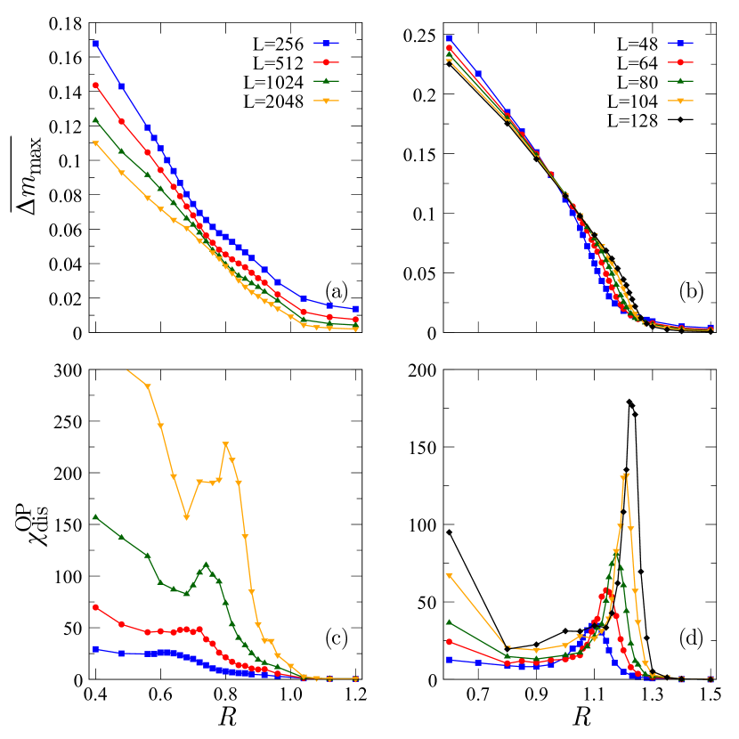
Figure 5: Disorder-averaged value of the order parameter, $\overline{\Delta m_{\rm max}}$, as a function of $R$ for several system sizes $L$ in $2d$ (a) and $3d$ (b). The corresponding variance of $\Delta m_{\rm max}$ multiplied by $N=L^{d}$ is the disconnected susceptibility and is shown in $2d$ (c) and $3d$ (d).

.2.1 Order parameters

The disorder-controlled transition from a discontinuous behavior of the magnetization curve to a continuous behavior can be characterized by several choices of order parameter. The most obvious one is the maximum magnetization jump, $\Delta m_{\rm max}=\max_{t}\{\Delta m_{t}\}$, where $\Delta m_{t}=m_{t+1}-m_{t}$. This is the analog of the maximum stress drop $\Delta\sigma_{\rm max}$ used in Refs. [Ozawa et al., 2018, 2020; Bhaumik et al., 2021]. We compute its disorder-averaged value, $\overline{\Delta m_{\rm max}}$, and its variance, ${\rm Var}(\Delta m_{\rm max})=\left(\overline{\Delta m_{\rm max}^{2}}-\overline{\Delta m_{\rm max}}^{2}\right)$, from which we define the disconnected susceptibility as $\chi^{\rm OP}_{\rm dis}(R,L)=L^{d}{\rm Var}(\Delta m_{\rm max})$. As in the main text, the overline denotes an average over samples, i.e., realizations of the random fields. The outcome is displayed in Fig. 5 for $2d$ and $3d$ and we see that the disconnected susceptibility shows a peak that grows with the system size at the onset of the growth of $\overline{\Delta m_{\rm max}}$, which is a hallmark of a critical transition.

However, as we decrease $R$ further, the variance starts to increase again with the system size. This unexpected behavior can be explained by the following argument. When $R\to 0$, there are no spin flips as $H$ increases until the discontinuous jump at the coercive field $H_{\rm co}$. At $H_{\rm co}$, a single site $i^{*}$ with the largest random field initiates the macroscopic jump. We thus define the maximum random field by $h_{\rm max}=h_{i^{*}}=\max_{i}\{h_{i}\}$. According to Eq. (5), when $R\to 0$, $H_{\rm co}$ and $h_{\rm max}$ are related by

$$0=h_{i^{*}}^{\rm eff}=-\sum_{j\neq i^{*}}G_{i^{*}j}+h_{i^{*}}+H_{\rm co},$$ (13)

where we have used that $s_{j\neq i^{*}}=-1$. Since $\sum_{i}G_{ij}=\hat{G}_{{\bf q}={\bf 0}}=0$ and $G_{ii}=0$ by definition, we arrive at $H_{\rm co}=-h_{\rm max}$. As also described in the main text, the magnetization $m$ grows linearly with the external field $H$ beyond $H_{\rm co}$, due to the propagation of the band in the transverse direction. This allows us to write the evolution of $m$ when $R\to 0$ as

$$m(H)=\begin{cases}-1\ ,&H<H_{\rm co},\\ AH+B,&H\geq H_{\rm co},\end{cases}$$ (14)

where $A$ and $B$ are some constants. Thus, we obtain $\Delta m_{\rm max}=m(H_{\rm co})+1=AH_{\rm co}+B+1$. We can then relate the variance of $\Delta m_{\rm max}$, $H_{\rm co}$, and $h_{\rm max}$ through

$${\rm Var}(\Delta m_{\rm max})=A^{2}\,{\rm Var}(H_{\rm co})=A^{2}\,{\rm Var}(h_{\rm max}).$$

We assumed that sample-to-sample fluctuations solely come from $H_{\rm co}$, which is confirmed numerically. Since the initial distribution of $h_{i}$ is Gaussian, $h_{\rm max}$ follows a Gumbel distribution, associated with extreme-value statistics Fortin and Clusel (2015). We then arrive at

$$\chi^{\rm OP}_{\rm dis}(R,L)=N{\rm Var}(\Delta m_{\rm max})=\frac{A^{2}\pi^{2}R^{2}N}{12\ln N}\ ,$$ (15)

with $N=L^{d}$. This expression explains the peculiar growth of the variance with $L$ when $R$ gets smaller in Fig. 5(c, d). This effect appears much more pronounced in the $2d$ case.

To avoid the above problem, which is an artifact of lattice-based modeling, we introduce an alternative order parameter. As discussed in the main text for the description of the discontinuous regime at small disorder, we monitor the mean magnetization along horizontal and vertical lines (in $2d$) or planes (in $3d$),

$$m_{x} =\frac{1}{L}\sum_{y=1}^{L}s_{(x,y)}\qquad(2d),$$ (16)

$$m_{x} =\frac{1}{L^{2}}\sum_{y,z=1}^{L}s_{(x,y,z)}\qquad(3d),$$ (17)

and similarly for $m_{y}$ (and $m_{z}$ in $3d$). When the disorder strength $R$ is large, spins flip rather homogeneously in space, and no noticeable difference is observed between these quantities, e.g., in $3d$, between $m_{x}$, $m_{y}$, and $m_{z}$ whatever $x,y,z$. On the other hand, when $R$ is small, a sharp band emerges, causing a strong localization and anisotropy of spin flips. In such a situation, there is some location, say $x^{*}$, for which $m_{x^{*}}\simeq 1$ right after the macroscopic magnetization jump. Thus, we monitor at each step $t$ of the evolution (see Sec. .1.1) $m_{\rm b,t}=\max_{x,y}\{m_{x,t},m_{y,t}\}$, or its counterpart in $3d$, which precisely detects the emergence of a band at $H_{\rm co}$ (if present). Some representative magnetization curves $m(H)$ for various $R$ and the corresponding $m_{\rm b}(H)$ are shown in Fig. 6.

To characterize the disorder-controlled transition between the discontinuous and continuous regimes, and as we did for the magnetization, we then compute the maximum jump as $\Delta m_{\rm b,max}=\max_{t}\{\Delta m_{\rm b,t}\}$ with $\Delta m_{\rm b,t}=m_{\rm b,t+1}-m_{\rm b,t}$ for each sample realization. From this we define the sample-average order parameter $\overline{\Delta m_{\rm b,max}}$ and the associated disconnected susceptibility $\chi^{\rm OP}_{\rm dis,b}(R,L)=L^{d-1}{\rm Var}(\Delta m_{\rm b,max})$.

Note that the disconnected susceptibilities defined from either $m_{\rm b}(H)$ or $\Delta m_{\rm b,max}$ are equal to the variance multiplied by $L^{d-1}$ and not by $N=L^{d}$ as for the magnetization and its maximum jump. The difference is due to the fact that $m$ is a volume-averaged quantity in each sample whereas $m_{\rm b}$ is a line- or plane-averaged quantity. In the limit where all spins are uncorrelated, it is easy to see that the so-defined disconnected susceptibilities are of O(1), which provides the proper baseline for studying their peak.

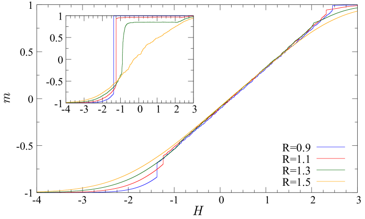
Figure 6: Magnetization curves $m(H)$ for $3d$ samples with $L=104$ and different values of $R$. Insets: The corresponding $m_{\rm b}(H)$ curves.

.2.2 Discontinuous regime

Before discussing the disorder-controlled transition we first illustrate the existence of a discontinuous regime at small disorder. As mentioned in the main text the magnetization discontinuity observed in each sample is rounded when one averages over samples. One then has to proceed to a finite-size scaling analysis to check whether the discontinuity reappears in the thermodynamic limit. We compute the disconnected and connected susceptibilities associated with the two order parameters $m(H)$ and $m_{\rm b}(H)$,

$$\chi_{\rm dis}(H)=L^{d}{\rm Var}(m(H)),$$ (18)

$$\chi_{\rm con}(H)=\frac{\partial\overline{m(H)}}{\partial H},$$

$$\chi_{\rm dis,b}(H)=L^{d-1}{\rm Var}(m_{\rm b}(H)),$$

$$\chi_{\rm con,b}(H)=\frac{\partial\overline{m_{\rm b}(H)}}{\partial H},$$

for a small $R$ and for several system sizes $L$. We illustrate in Fig. 7 the outcome for the susceptibilities associated with $m_{\rm b}(H)$ for $R=0.64$ in $2d$ and $R=1.05$ in $3d$. We can see that the suceptibilities peak at a well-defined coercive field $H_{\rm co}(L)$ and that the peak sharpens and gets higher as $L$ increases. We find that the peak maximum of $\chi_{\rm dis,b}$ grows as $L^{d-1}$ both in $2d$ and $3d$ while the maximum of $\chi_{\rm con,b}$ grows with $L$ with smaller exponents due to the sample-to-sample fluctuations of $H_{\rm co}$ Ozawa et al. (2020): see the insets. A similar behavior is found for the susceptibilities associated with $m(H)$ except that the peak of $\chi_{\rm dis}(H)$ grows as $L^{d}$.

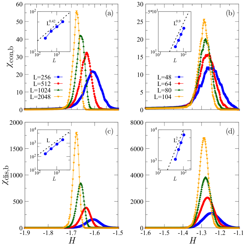
Figure 7: Weak-disorder regime: Finite-size scaling analysis of the disconnected and connected susceptibilities $\chi_{\rm con,b}(H,L)$ (top) and $\chi_{\rm dis,b}(H,L)$ (bottom) in $2d$ for $R=0.64$ (left) and in $3d$ for $R=1.05$ (right). Insets: log-log plot of the susceptibility peak versus system size $L$. The peak of the disconnected ones grows with an exponent $d-1$ and that of the connected one with an exponent around $0.42$ in $2d$ and $0.9$ in $3d$.

.2.3 Disorder-controlled transition

To characterize the critical behavior (exponents and scaling functions) from a finite-size scaling analysis, we have used several methods based on the scaling ansatz described in the main text [see the relations in Eq. (2)]. Note that extracting the critical properties from finite-size studies is much more demanding (and as a result less accurate) for a far-from-equilibrium critical point in a disordered system than for conventional critical points in pure systems at equilibrium. It indeed lacks the symmetries (time-reversal, inversion) of the equilibrium ones and is affected by strong corrections to scaling. This has been vividly illustrated in the case of scaling analyses of the mean-field driven RFIM, whose analytical solution is otherwise exactly known Perkovic et al. (1996); *perkovic1999.

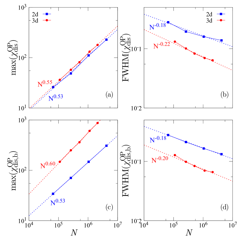
Figure 8: Log-log plot of the height (left) and width (right) of the $R$-dependent disconnected susceptibilities $\chi_{\rm dis}^{\rm OP}(R,L)$ (top) and $\chi_{\rm dis,b}^{\rm OP}(R,L)$ (bottom) as a function of the system size $N=L^{d}$ in $2d$ and $3d$.

The first method we used is to consider the height and the width of the $R$-dependent disconnected susceptibilities $\chi_{\rm dis}^{\rm OP}(R,L)$ and $\chi_{\rm dis,b}^{\rm OP}(R,L)$ as a function of the system size: The height is expected to grow as $L^{\bar{\gamma}/\nu}$ or $L^{\bar{\gamma}_{\rm b}/\nu}$ and the width to decay as $L^{-1/\nu}$. We show a log-log plot of the dependence on $N=L^{d}$ for both $2d$ and $3d$ in Fig. 8. This allows us to estimate the critical exponents as: $\bar{\gamma}/\nu\approx 1.07\pm 0.03$, $\bar{\gamma}_{\rm b}/\nu\approx 1.060\pm 0.002$, $\nu\approx 2.74\pm 0.05$ in $2d$ and $\bar{\gamma}/\nu\approx 1.65\pm 0.06$, $\bar{\gamma}_{\rm b}/\nu\approx 1.82\pm 0.05$, and $\nu\approx 1.64\pm 0.06$ in $3d$, where the error bars are derived from the fits. We have also checked that a similar procedure applied to the maximum over $H$ of the disconnected susceptibility $\chi_{\rm dis,b}(H,L)$ evaluated for $R=R_{c}(L)$ gives compatible results ($\bar{\gamma}_{\rm b}/\nu$ between 0$.95$ and $1.2$ in $2d$ and $\bar{\gamma}_{\rm b}/\nu\approx 1.80\pm 0.03$ in $3d$), as illustrated in Fig. 9.

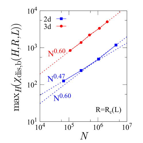
Figure 9: Log-log plot of the height of the maximum over $H$ of the disconnected susceptibility $\chi_{\rm dis,b}(H,R,L)$ at $R=R_{c}(L)$ as a function of $N=L^{d}$ in $2d$ and $3d$.

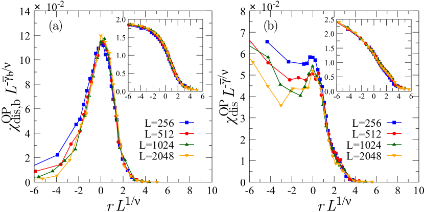
Figure 10: Finite-size scaling collapse of the disconnected susceptibilities $\chi^{\rm OP}_{\rm dis,b}(r,L)$ with $\bar{\gamma}_{\rm b}/\nu=1.03$ (a) and $\chi^{\rm OP}_{\rm dis}(r,L)$ with $\bar{\gamma}/\nu=1.1$ (b) in $2d$, where $r=(R-R_{c}(L))/R$. Insets: Same for $\overline{\Delta m_{\rm b,max}}$ with $\beta_{\rm b}/\nu=0.0$ (a) and $\overline{\Delta m_{\rm max}}$ with $\beta/\nu=0.46$ (b). In all cases $\nu=2.7$.

We next perform scaling collapses to the expressions in Eq. (2) of the main text, where the exponents and the critical disorder $R_{c}(L)$ are adjusted to provide the best visual collapse of the curves obtained for different values of $L$. This gives values that are consistent with the previous ones, $\bar{\gamma}/\nu\approx 1.1\pm 0.05$, $\bar{\gamma}_{\rm b}/\nu\approx 1.03\pm 0.03$, $\nu\approx 2.7\pm 0.1$ in $2d$ and $\bar{\gamma}/\nu\approx 1.70\pm 0.05$, $\bar{\gamma}_{\rm b}/\nu\approx 1.81\pm 0.05$, and $\nu\approx 1.8\pm 0.6$ in $3d$. In addition, from the collapse of the disorder-averaged order parameters, we also obtain $\beta/\nu\approx 0.46\pm 0.02$, $\beta_{\rm b}/\nu\approx 0.0\pm 0.02$, $\nu\approx 2.7\pm 0.2$ in $2d$, and $\beta/\nu\approx 0.62\pm 0.04$, $\beta_{\rm b}/\nu\approx 0.08\pm 0.04$, and $\nu\approx 1.4\pm 0.4$ in $3d$. The results are shown for $3d$ in the main text and we give here their $2d$ counterparts: see Fig. 10.

We also fit the disconnected susceptibility data to a flexible functional form of master-curve to extract the universal scaling function. To start with, we use a nonlinear fit with a Gaussian around the peak of the susceptibility curves to get an estimate of the value of $R_{c}(L)$. We find that the estimated value is very close to the one obtained by simply looking at the peak position (see above). Following the same procedure as in Ref. [Shekhawat et al., 2013] we fit the curves for $\chi_{\rm dis,b}^{\rm OP}(r,L)$ with $A_{\rm b}L^{\bar{\gamma}_{\rm b}/\nu}\bar{\Psi}_{\rm b}(\alpha_{\rm b}rL^{1/\nu})$, where we choose

$$\bar{\Psi}_{\rm b}(x)=\exp{(x-\exp{(x)})}\left(1+\sum_{i=1}^{3}a_{{\rm b},i}H_{i}(x)\right),$$ (19)

with $H_{i}(x)$ the $i$-th Hermite polynomial and $\bar{\gamma}_{\rm b}/\nu$, $\nu$, $A_{\rm b}$, $\alpha_{\rm b}$, and $a_{{\rm b},i}$ ($i=1,2,3$) are adjustable parameters. $A_{\rm b}$ and $\alpha_{\rm b}$ control the axis scales and are irrelevant for the universality class, while the $a_{{\rm b},i}$’s describe the curve shape and should be universal. To reduce the effect of the scaling corrections at smaller sizes we only fit systems with $L\geq 1024$ in $2d$ and $L\geq 80$ in $3d$. We then find $\bar{\gamma}_{\rm b}/\nu=1.07\pm 0.04$, $\nu=2.7\pm 0.4$ for $2d$ and $\bar{\gamma}_{\rm b}/\nu=1.87\pm 0.03$ and $\nu=1.6\pm 0.4$ for $3d$.

Finally, we have considered the shift of the critical disorder and fitted it to $R_{c}(\infty)-R_{c}(L)\propto L^{-1/\nu}$. This is described in Sec. .3.

.2.4 Comparison with elasto-plastic models

To investigate whether the critical points of the RFIM-Eshelby and of the mesoscopic models for sheared amorphous solids known as elasto-plastic models (EPMs) are in the same universality class we have compared the scaling functions for the disconnected susceptibilities.

We first proceed to the same treatment as above with the parametrization in Eq. (19) to extract the scaling function of $\chi_{\rm dis,b}^{\rm OP}(R,L)$ (obtained from the variance of the maximum jump of the band order parameter $n_{\rm b}$ which is the counterpart of $m_{\rm b}$) for the EPM studied in Ref. [Rossi et al., 2022]. In this case we fit the curves in $2d$ for $L$ from $1024$ to $4096$ and in $3d$ for $L$ from $80$ to $164$. We plot the result for the scaling functions of the Eshelby-RFIM and the EPM in Figure 11. We see that the two models seem to have a very similar scaling function, but as discussed in the main text the exponent ratio $\bar{\gamma}_{\rm b}/\nu$ is about $10\%$ more in the RFIM.

We also perform a direct comparison of the disconnected susceptibility curves $\chi_{\rm dis}^{\rm OP}(r,L)$ built from the maximum magnetization jump (RFIM) or from the maximum stress drop (EPM) for $2d$ and $3d$. We collapse all the curves by using the same exponents for the Eshelby-RFIM and the EPM, namely, $\bar{\gamma}/\nu=1.05$ and $\nu=2.7$ in $2d$ and $\bar{\gamma}/\nu=1.75$ and $\nu=1.6$ in $3d$. As seen in Fig. 12, the collapse appears very good in $3d$ (less so in $2d$ where the curves are significantly affected by the extreme-value statistics at low disorder). These data also suggest that the two models are in the same universality class.

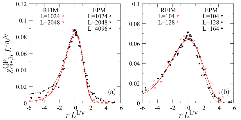
Figure 11: Comparison of the scaling functions for the disconnected susceptibility $\chi_{\rm dis,b}^{\rm OP}(r,L)$ of the Eshelby-RFIM (red) and of the elasto-plastic model of Ref. [Rossi et al., 2022] (black) in $2d$ (left) and $3d$ (right). The full red (dashed black) line is the fitted functional form of Eq. (19) to the data coming from the Eshelby-RFIM (EPM), and the data are only shown for $L\geq 1024$ in $2d$ and $L\geq 104$ in $3d$. The ratio $\bar{\gamma}_{\rm b}/\nu$ used for the collapse is $10\%$ higher in the Eshelby-RFIM.

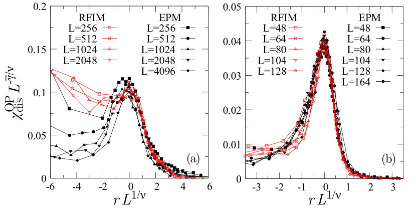
Figure 12: Finite-size scaling collapse of the disconnected susceptibility curves $\chi_{\rm dis}^{\rm OP}(r,L)$ for the Eshelby-RFIM (empty symbols, red) and the elasto-plastic model of Ref. [Rossi et al., 2022] (full symbols, black) in $2d$ (left) and $3d$ (right). The collapse is obtained by using the same exponents for the two models: $\bar{\gamma}/\nu=1.0$ and $\nu=2.7$ in $2d$, $\bar{\gamma}/\nu=1.75$ and $\nu=1.6$ in $3d$.

.3 Bounding the location of the disorder-controlled critical point

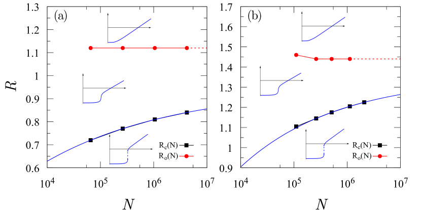
Figure 13: The critical point, $R_{c}(N)$, as a function of the system size, $N=L^{d}$, together with the value of the disorder $R_{o}(N)$ at which an overshoot first appears in the transformed magnetization curve $\tilde{\sigma}(H,N)$ for the $2d$ (a) and the $3d$ (b) cases. Blue curves are fits to $R_{c}(\infty)-R_{c}(N)=aN^{-b}$, with $a$, $b$, and $R_{c}(\infty)$ taken as adjustable parameters and given in the text. Insets: The corresponding schematic magnetization curves.

Figure 13 presents $R_{c}(N)$ as a function of $N=L^{d}$ in both $2d$ and $3d$, showing a slow monotonic increase of $R_{c}(N)$ with $N$. We now provide evidence that $R_{c}$ remains finite in the thermodynamic limit. Note that the fate of the critical point in the thermodynamic limit has been a key issue in the study of yielding in amorphous materials Barlow et al. (2020); Richard et al. (2021); Rossi et al. (2022). As discussed above, a standard finite-size scaling argument suggests that $R_{c}(\infty)-R_{c}(L)\propto L^{-1/\nu}$. Through a direct fit of $R_{c}(\infty)-R_{c}(N)=aN^{-b}$, with $a$, $b$ and $R_{c}({\infty})$ adjustable parameters, we find $R_{c}({\infty})=0.95$, $a=1.65$, $b=0.178$ in $2d$ and $R_{c}({\infty})=1.35$, $a=3.97$, $b=0.237$ in $3d$. The parameter $b$ is related to the critical exponent $\nu$ through $b=1/(d\nu)$, which yields $\nu\approx 2.80$ in $2d$ and $\nu\approx 1.41$ in $3d$, values which are compatible with the independent finite-size analysis performed above.

To go beyond this fit and more firmly establish that $R_{c}(\infty)$ has a finite value, we estimate an upper bound following the method devised in the study of yielding in an EPM Rossi et al. (2022). In the latter we monitored the value $R_{o}(N)$ at which an overshoot, i.e., a local maximum, first appears in the disorder-averaged stress ($\sigma$) versus strain ($\gamma$) curve. This value is always an upper bound of the critical disorder. We found that $R_{o}(N)$ is independent of $N$ over the whole accessible range of system sizes both in $2d$ and $3d$ Rossi et al. (2022). To repeat this analysis in the case of the Eshelby-RFIM we first build on the analogy between the two models already described in the main text. As illustrated in Fig. 1 of the main text and here in Fig. 6, the magnetization follows a linear regime $m(H)=AH+B$ (with $A$ and $B$ weakly $R$-dependent) before saturating to $+1$ at large applied field $H$. When plotting the quantity $\tilde{\sigma}(H)=AH-m(H)$ we can see that it qualitatively reproduces the stress-strain curve $\sigma(\gamma)$ of the EPM with the same evolution as a function of disorder strength: see Fig. 14(a) for an illustration in $3d$. From the average over samples of these transformed magnetization curves we then identify the onset $R_{o}(N)$ at which a local maximum (overshoot) first appears in $\tilde{\sigma}(H,R)$, as shown in Fig. 14(b). The outcome is plotted in Fig. 13 and we find that, as for the EPM, $R_{o}(N)$ is essentially independent of $N$ and therefore provides a finite upper bound for the critical disorder $R_{c}(\infty)$.

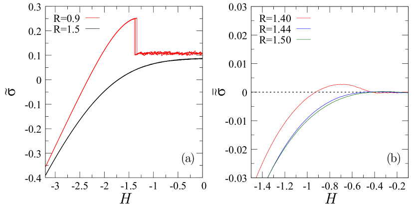
Figure 14: (a): The transformed magnetization curve, $\tilde{\sigma}(H)=AH-m(H)$, for the $3d$ Eshelby-RFIM with a small and a large disorder strength $R$ (same samples as in Fig. 1(a) of the main text). Note the similarity with the stress-strain curves of a mesoscopic model of a uniformly sheared amorphous solid Rossi et al. (2022). (b): The onset value $R_{o}(L)$ at which a local maximum (overshoot) first appears is identified at $R_{o}\approx 1.5$ for $L=104$.

.4 Avalanches at small disorder: a comparison between the Eshelby-RFIM and the EPM

The evolution of AQS driven disordered systems proceeds by avalanches. We focus here on a comparative study of the Eshelby RFIM and the EPM of Ref. [Rossi et al., 2022] in the small-disorder regime, away from the disorder-controlled critical point. The EPM is considered at large enough imposed strain, beyond the yielding transition and the Eshelby-RFIM in the linear regime beyond the coercive field $H_{\rm co}$ and well before the saturation to a magnetization $m=+1$.

We study the distribution of avalanche sizes $P(S)$ for a given (small) $R$ and cumulated along a significant fraction of the linear regime between two values, $m_{\rm min}$ and $m_{\rm max}$, of the average magnetization. The size $S$ of an avalanche is defined as $N$ times the associated jump $\delta m$ of the sample-dependent magnetization and $P(S)$ is normalized. In AQS driven disordered systems one commonly encounters a scaling behavior of the form

$$P(S)\sim S^{-\tau}\mathcal{P}(S/S_{c}),$$ (20)

with $\tau$ an exponent and $\mathcal{P}$ a scaling function that decreases very quickly for $S>S_{c}$. In a finite system of linear size $L$, the cutoff avalanche size $S_{c}$ can either be independent of $L$ or, in the presence of criticality (either disorder-controlled, self-organized, or due to marginal stability), grow as $S_{c}\sim L^{d_{f}}$, where $d_{f}$ is the fractal dimension of the largest avalanches. This can be probed by computing $P(S)$ and trying to collapse all the curves on a plot of $P(S)L^{\tau d_{f}}$ vs $S/L^{d_{f}}$ by adjusting $\tau$ and $d_{f}$. These exponents have been extensively studied for various AQS driven disordered solids such as the ferromagnetic RFIM at criticality Perkovic et al. (1996); *perkovic1999; Pérez-Reche and Vives (2003, 2004), elastic manifolds at their depinning transition (for a review, see [Wiese, 2022]), or sheared amorphous solids Salerno and Robbins (2013); Lin et al. (2014a); Nicolas et al. (2018).

In the EPM description of sheared amorphous solids in their steady state, these scale-free avalanches are associated with a marginal stability according to which there exists a pseudo-gap in the distribution of the local stability, $\tilde{P}(x)\sim x^{\theta}$ with $\theta>0$ Lerner and Procaccia (2009); Lin et al. (2014a). This property also translates in the distribution of the strain intervals between two successive avalanches $Q(\delta\gamma)$, for which the corresponding average interval goes to zero with system size as $<\delta\gamma>\sim N^{-1/(1+\theta)}$. In $2d$ EPMs one finds $\theta\approx 0.5-0.6$ and in $3d$ $\theta\approx 0.3-0.45$ Lerner and Procaccia (2009); Lin et al. (2014a, b); Nicolas et al. (2018).

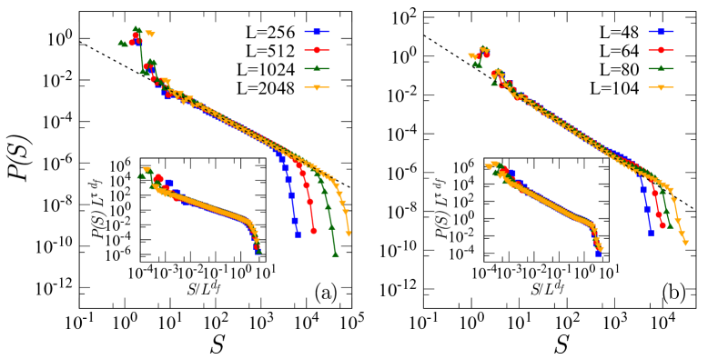
Figure 15: Finite-size scaling of the avalanche size distribution for $2d$ and $R=0.6$ (a) and $3d$ and R=0.8 (b). The vertical axis is shifted so that the large avalanches ($S\gtrsim 20$) fall as much as possible on the same curve, which is marked by a black dashed line. The insets show a further collapse by rescaling the axes. The collapse gives $\tau\approx 1.22$, $d_{f}\approx 1.3$ in $2d$ and $\tau\approx 1.58$, $d_{f}\approx 1.9$ in $3d$.

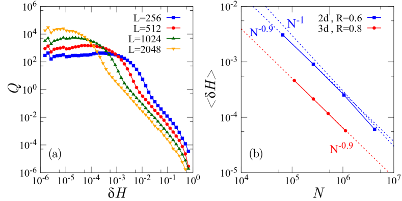
Figure 16: (a): Distribution $Q(\delta H,L)$ of the intervals between successive avalanches in the linear regime of the $2d$ Eshelby-RFIM with $R=0.6$. (b): Log-log plot of the average interval $<\delta H>$ versus $N$ for the same case and for the $3d$ version at $R=0.8$. The dashed lines indicate $N^{-1}$ and $N^{-0.9}$ for $2d$ and $N^{-0.9}$ for $3d$.

We have tested our procedure to determine the avalanche size distribution $P(S)$ and the distribution of intervals between successive avalanches $Q(\delta\gamma)$ for the EPM already studied in Ref. [Rossi et al., 2022] and we have properly recovered the results of the existing literature. We have then applied the same treatment to the Eshelby-RFIM in the linear regime of the magnetization curve. A difficulty, however, is that there seems to be a different behavior of the small (say, $S\lesssim 20$) and the large ($S\gtrsim 20$) avalanches as the system size increases. One possible explanation is that because the interactions are not purely ferromagnetic in the Eshelby-RFIM, a spin can flip more than once. In the case of a $1d$ long-ranged anti-ferromagnetic RFIM, this was shown to lead to different types of avalanches with different characteristicsNampoothiri et al. (2017). However, in the present case we find that spins flip usually once and at most a few number of times. To nonetheless see if there is a difference between avalanches involving a change of magnetization and avalanches in which spin flips do not change the magnetization we have considered a measure of the avalanche size by the number of spin flips, but we have obtained essentially the same result as with the magnetization jumps. One can try to somehow overlook the small avalanches (despite the fact that their number grows with the system size) by collapsing the avalanche distribution only in the range of the large avalanches: this is shown in Fig. 15 for weak disorder in $2d$ and $3d$. One can fit a power law over some range with exponent $\tau\approx 1.2$ in $2d$ and $1.6$ in $3d$, and the cutoff avalanche size seems to grow with $L$.

We have also monitored the distribution of intervals between avalanches, $Q(\delta H,L)$, and computed the average $<\delta H>$. The distribution is displayed in Fig. 16(a) and the average interval versus system size is shown on a log-log plot in Fig. 16(b). We find that $<\delta H>$ varies very weakly with $L$, which would predict an exponent $\theta\sim 0-0.1$, barely compatible with any marginal stability. (In $3d$, we find $\theta\approx 0.1$.)

Although a more exhaustive investigation taking into account the properties of the different types of avalanches and of intervals $\delta H$ would be required, our results seem to indicate that EPMs and RFIMs away from the disorder-controlled critical point display different types of behavior as far as avalanches, marginal stability, and of course the existence or not of a bona fide steady state, are concerned. This appears likely due to the possibility or not for sites to be active an arbitrary large number of times.

References

- Fisher (1998) D. S. Fisher, Physics Reports 301, 113–150 (1998).
- Sethna et al. (2001) J. P. Sethna, K. A. Dahmen, and C. R. Myers, Nature 410, 242 (2001).
- Alava et al. (2006) M. J. Alava, P. K. V. V. Nukala, and S. Zapperi, Advances in Physics 55, 349–476 (2006), https://doi.org/10.1080/00018730300741518 .
- Dahmen and Ben-Zion (2011) K. A. Dahmen and Y. Ben-Zion, “Jerky motion in slowly driven magnetic and earthquake fault systems, physics of,” in Extreme Environmental Events: Complexity in Forecasting and Early Warning, edited by R. A. Meyers (Springer New York, 2011) p. 680–696.
- Sethna et al. (2017) J. P. Sethna, M. K. Bierbaum, K. A. Dahmen, C. P. Goodrich, J. R. Greer, L. X. Hayden, J. P. Kent-Dobias, E. D. Lee, D. B. Liarte, X. Ni, K. N. Quinn, A. Raju, D. Z. Rocklin, A. Shekhawat, and S. Zapperi, Annual Review of Materials Research 47, 217 (2017), https://doi.org/10.1146/annurev-matsci-070115-032036 .
- Perez-Reche (2017) F. J. Perez-Reche, “Modelling avalanches in martensites,” in Avalanches in Functional Materials and Geophysics, edited by E. K. Salje, A. Saxena, and A. Planes (Springer International Publishing, 2017) p. 99–136.
- Wiese (2022) K. J. Wiese, Reports on Progress in Physics 85, 086502 (2022).
- Bak et al. (1987) P. Bak, C. Tang, and K. Wiesenfeld, Phys. Rev. Lett. 59, 381 (1987).
- Bak et al. (1988) P. Bak, C. Tang, and K. Wiesenfeld, Phys. Rev. A 38, 364 (1988).
- Müller and Wyart (2015) M. Müller and M. Wyart, Annual Review of Condensed Matter Physics 6, 177 (2015), https://doi.org/10.1146/annurev-conmatphys-031214-014614 .
- Thomas Nattermann et al. (1992) Thomas Nattermann, Semjon Stepanow, Lei-Han Tang, and Heiko Leschhorn, J. Phys. II France 2, 1483–1488 (1992).
- Sethna et al. (1993) J. P. Sethna, K. Dahmen, S. Kartha, J. A. Krumhansl, B. W. Roberts, and J. D. Shore, Phys. Rev. Lett. 70, 3347 (1993).
- Sethna et al. (2006) J. P. Sethna, K. A. Dahmen, and O. Perkovic, in The Science of Hysteresis, edited by G. Bertotti and I. D. Mayergoyz (Academic Press, 2006) p. 107–179.
- Rodney et al. (2011) D. Rodney, A. Tanguy, and D. Vandembroucq, Modelling and Simulation in Materials Science and Engineering 19, 083001 (2011).
- Kumar et al. (2013) G. Kumar, P. Neibecker, Y. H. Liu, and J. Schroers, Nature communications 4, 1 (2013).
- Vasoya et al. (2016) M. Vasoya, C. H. Rycroft, and E. Bouchbinder, Physical Review Applied 6, 024008 (2016).
- Fan et al. (2017) M. Fan, M. Wang, K. Zhang, Y. Liu, J. Schroers, M. D. Shattuck, and C. S. O’Hern, Physical Review E 95, 022611 (2017).
- Ozawa et al. (2018) M. Ozawa, L. Berthier, G. Biroli, A. Rosso, and G. Tarjus, Proceedings of the National Academy of Sciences 115, 6656 (2018).
- Ozawa et al. (2020) M. Ozawa, L. Berthier, G. Biroli, and G. Tarjus, Physical Review Research 2, 023203 (2020).
- Barlow et al. (2020) H. J. Barlow, J. O. Cochran, and S. M. Fielding, Physical Review Letters 125, 168003 (2020).
- Richard et al. (2021) D. Richard, C. Rainone, and E. Lerner, The Journal of Chemical Physics 155, 056101 (2021).
- Pollard and Fielding (2022) J. Pollard and S. M. Fielding, Physical Review Research 4, 043037 (2022).
- Rossi et al. (2022) S. Rossi, G. Biroli, M. Ozawa, G. Tarjus, and F. Zamponi, Phys. Rev. Lett. 129, 228002 (2022).
- Rossi and Tarjus (2022) S. Rossi and G. Tarjus, Journal of Statistical Mechanics: Theory and Experiment 2022, 093301 (2022).
- Borja da Rocha and Truskinovsky (2020) H. Borja da Rocha and L. Truskinovsky, Phys. Rev. Lett. 124, 015501 (2020).
- Eshelby (1957) J. D. Eshelby, Proceedings of the royal society of London. Series A. Mathematical and physical sciences 241, 376 (1957).
- Picard et al. (2004) G. Picard, A. Ajdari, F. Lequeux, and L. Bocquet, The European Physical Journal E 15, 371 (2004).
- Nicolas et al. (2018) A. Nicolas, E. E. Ferrero, K. Martens, and J.-L. Barrat, Reviews of Modern Physics 90, 045006 (2018).
- Magni (1999) A. Magni, Physical Review B 59, 985 (1999).
- Kurbah and Shukla (2011) L. Kurbah and P. Shukla, Phys. Rev. E 83, 061136 (2011).
- Nampoothiri et al. (2017) J. N. Nampoothiri, K. Ramola, S. Sabhapandit, and B. Chakraborty, Phys. Rev. E 96, 032107 (2017).
- (32) J. P. Sethna, K. A. Dahmen, and O. Perkovic, arXiv preprint cond-mat/0406320 .
- Dubey et al. (2015) A. K. Dubey, H. G. E. Hentschel, P. K. Jaiswal, C. Mondal, I. Procaccia, and B. S. Gupta, Europhysics Letters 112, 17011 (2015).
- Pérez-Reche and Vives (2003) F. J. Pérez-Reche and E. Vives, Phys. Rev. B 67, 134421 (2003).
- Pérez-Reche and Vives (2004) F. J. Pérez-Reche and E. Vives, Phys. Rev. B 70, 214422 (2004).
- Note (1) It has been argued in Ref. [\rev@citealpnumprocaccia_screening] that the long-range decay of the Eshelby kernel is actually screened by the presence of emergent dipoles.Work is in progress to test the robustness of our results to the range of the quadrupole-quadrupole interaction.
- Note (2) Although hard to prove directly, a first hint in this direction is provided by the behavior of the system-spanning band in the discontinuous regime: it is clearly anisotropic but, as shown above, its size nonetheless scales linearly with both in the longitudinal and the transverse direction.
- Shekhawat et al. (2013) A. Shekhawat, S. Zapperi, and J. P. Sethna, Phys. Rev. Lett. 110, 185505 (2013).
- Spasojević et al. (2011) D. Spasojević, S. Janićević, and M. Knežević, Physical review letters 106, 175701 (2011).
- Hayden et al. (2019) L. X. Hayden, A. Raju, and J. P. Sethna, Physical Review Research 1, 033060 (2019).
- Note (3) Note that the EPM exponent was defined differently in Ref. [\rev@citealpnumrossi2022finite] and shifted by because of a different definition of .
- Perkovic et al. (1996) O. Perkovic, K. A. Dahmen, and J. P. Sethna, (1996), arXiv:cond-mat/9609072 [cond-mat] .
- Perković et al. (1999) O. Perković, K. A. Dahmen, and J. P. Sethna, Phys. Rev. B 59, 6106 (1999).
- Mondal et al. (2023) C. Mondal, M. Moshe, I. Procaccia, and S. Roy, (2023), arXiv:2305.11253 [cond-mat.soft] .
- Maloney and Lemaitre (2006) C. E. Maloney and A. Lemaitre, Physical Review E 74, 016118 (2006).
- Ferrero and Jagla (2019) E. E. Ferrero and E. A. Jagla, Soft matter 15, 9041 (2019).
- Budrikis and Zapperi (2013) Z. Budrikis and S. Zapperi, Phys. Rev. E 88, 062403 (2013).
- Bhaumik et al. (2021) H. Bhaumik, G. Foffi, and S. Sastry, Proceedings of the National Academy of Sciences 118 (2021).
- Fortin and Clusel (2015) J.-Y. Fortin and M. Clusel, Journal of Physics A: Mathematical and Theoretical 48, 183001 (2015).
- Salerno and Robbins (2013) K. M. Salerno and M. O. Robbins, Phys. Rev. E 88, 062206 (2013).
- Lin et al. (2014a) J. Lin, E. Lerner, A. Rosso, and M. Wyart, Proceedings of the National Academy of Sciences 111, 14382 (2014a).
- Lerner and Procaccia (2009) E. Lerner and I. Procaccia, Phys. Rev. E 79, 066109 (2009).
- Lin et al. (2014b) J. Lin, A. Saade, E. Lerner, A. Rosso, and M. Wyart, EPL (Europhysics Letters) 105, 26003 (2014b).