Robustness of the Random Language Model

Abstract

The Random Language Model (De Giuli 2019) is an ensemble of stochastic context-free grammars, quantifying the syntax of human and computer languages. The model suggests a simple picture of first language learning as a type of annealing in the vast space of potential languages. In its simplest formulation, it implies a single continuous transition to grammatical syntax, at which the symmetry among potential words and categories is spontaneously broken. Here this picture is scrutinized by considering its robustness against explicit symmetry breaking, an inevitable component of learning in the real world. It is shown that the scenario is robust to such symmetry breaking. Comparison with human data on the clustering coefficient of syntax networks suggests that the observed transition is equivalent to that normally experienced by children at age 24 months.

Language is a way to convey complex ideas, instructions, and structures through sequences. Ubiquitous in everyday life, it also has a central role in computer science and molecular biology. One can ask if these disparate applications of language have any common features. The answer apparently is positive: the formalism of generative grammar, due to Post and Chomsky Post (1943); Chomsky (2002), though initially developed for human language, was immediately applied to computer languages, where it has remained important Hopcroft et al. (2007), and has also been applied to the molecular languages spoken by the cell Searls (2002); Knudsen and Hein (2003). Other idiosyncratic applications highlight the flexibility of the approach Escudero (1997).

Generative grammar models the syntax of language by a set of rules which, upon repeated application, yield ‘grammatical’ sentences. In this framework, for any grammatical sentence, there is a latent ‘derivation’ structure that encodes the syntax of that sentence; some examples are shown in Fig. 1.

Research on generative grammars in the computer science and linguistics literature focuses on classifications of grammars based on the complexity of the rules, corresponding classifications on the types of simple computers (automata) that can read their languages, and algorithms to parse text. Many results exist on the time and resource cost of parsing. Yet, if we admit that languages are always used by systems embedded in the physical world, then new questions arise: how much energy does it take to parse a grammar of a given complexity? How does a child navigate the space of all potential languages to hone in on the one taught to them? More broadly, one can ask, in the spirit of statistical physics, whether large grammars will show universality of the same type familiar from equilibrium statistical mechanics.

As an inroad to these questions, in Ref.DeGiuli (2019) the senior author proposed a simple ensemble of context-free grammars, the class of grammars most relevant to human and computer language. In its stochastic version, a context-free grammar assigns a probability (or more generally a weight) to each rule. DeGiuli (2019) explored the information-theoretic properties of grammars as functions of the variance of rule weights, the number of hidden categories, and the number of words.

The main result of DeGiuli (2019) is that the entropy of text produced by a context-free grammar depends strongly on the variance of the weights, such that two regimes are seen: a simple one in which, despite the presence of stochastic rules, sentences are nearly indistinguishable from uniform random noise; and a complex one in which sentences convey information. The transition between these regimes could be understood as a competition between Boltzmann entropy and an energy-like quantity.

Figure 1: Illustrative derivation trees for (a) simple English sentence, and (b) RNA secondary structure (after Searls (2002)). The latter is a derivation of the sequence ‘gacuaagcugaguc’ and shows its folded structure. Terminal symbols are encircled. Figure reproduced from DeGiuli (2019).

This work left many questions open:

(i) is the schematic learning scenario of DeGiuli (2019) robust to inevitable complications of real-world human language learning, such as explicit symmetry breaking?

(ii) is the transition shown in DeGiuli (2019) a true thermodynamic phase transition in an appropriate thermodynamic limit?

(iii) can the RLM be solved analytically?

(iv) what are the energy costs of physical systems that use CFGs to produce text?

In this work we address (i) and (ii) and comment on (iii); (iv) will be addressed elsewhere. We first show how previous theory implies that the RLM transition can be reached by increasing the heterogeneity of surface rules, and confirm this numerically. Then we consider the learning problem and motivate the RLM with a bias. Simulating this, we see that the RLM transition is preserved, but shifted due to the bias. A simple theory can rationalize the initial onset of nontrivial sentence entropy. To compare with human data Corominas-Murtra et al. (2009) we measure the clustering coefficient of a sentence graph, constructed from sampled sentences. This clustering is small until the RLM transition, where it begins to grow. Such a growth in clustering is also observed in syntactic networks made from human data, and supports that the RLM transition is equivalent to that typically experienced by children around 24 months. Finally, we discuss these results in the light on linguistic theory on first language acquisition.

I Brief review of the Random Language Model

To establish notation, here we briefly review the RLM. CFGs are assumed to be in Chomsky normal form, so that rules either take one hidden symbol $a$ to two hidden symbols $b,c$, or one hidden symbol $a$ to an observable one, $B$. These are quantified by weights $M_{abc}$ and $O_{aB}$, respectively. For a sentence $o_{j},j=1,\ldots,\ell$ with derivation $\sigma_{j},j=1,\ldots,2\ell-1$ on the tree $\mathscr{T}$, define $\pi_{abc}(\sigma)$ as the (unnormalized) usage frequency of rule $a\to bc$ and $\rho_{aB}(\sigma,o)$ as the (unnormalized) usage frequency of $a\to B$. Then consider the energy function

$$E(\sigma,o;M,O)=-\sum_{a,b,c}\pi_{abc}\log M_{abc}-\sum_{a,B}\rho_{aB}\log O_{aB}.$$ (1)

The Boltzmann weight $e^{-\beta E}$ counts derivations with a multiplicative weight $(M_{abc})^{\beta}$ for each usage of the interior rule $a\to bc$, and weight $(O_{aB})^{\beta}$ for each usage of the surface rule $a\to B$. We furthermore assign a weight to the tree itself: if each hidden node gets a weight $q$ and each surface node gets a weight $p$, then a rooted tree with $\ell$ leaves gets a weight $q^{2\ell-1}p^{\ell}$. The relative probability $p/q$ controls the size of trees; as in DeGiuli (2019) we fix $q=1-p$ and set $p=1/2+\epsilon$ where $\epsilon\ll 1$ to get large trees.

The RLM is an ensemble over CFGs. In DeGiuli (2019) it was argued that a generic model will have lognormally distributed weights, viz.,

$$\mathbb{P}_{G}(M,O) \equiv Z_{G}^{-1}\;J\;e^{-\epsilon_{d}s_{d}}e^{-\epsilon_{s}s_{s}}$$ (2)

where $s_{d}$ and $s_{s}$ are defined by

$$s_{d}=\frac{1}{N^{3}}\sum_{a,b,c}\log^{2}\left[\frac{M_{abc}}{\overline{M}}\right],\;\;s_{s}=\frac{1}{NT}\sum_{a,B}\log^{2}\left[\frac{O_{aB}}{\overline{O}}\right]$$ (3)

and $J=e^{-\sum_{a,b,c}\log M_{abc}-\sum_{a,B}\log O_{aB}}$. Here $\overline{M}=1/N^{2}$ and $\overline{O}=1/T$. It is straightforward to show that $\epsilon_{d}$ and $\epsilon_{s}$ satisfy

$$\overline{s_{d}}=(2\tilde{\epsilon}_{d})^{-1},\qquad\overline{s_{s}}=(2\tilde{\epsilon}_{s})^{-1}.$$ (4)

where $\overline{\;\cdot\;}$ denotes a grammar average and $\tilde{\epsilon}_{d}=\epsilon_{d}/N^{3}$, $\tilde{\epsilon}_{s}=\epsilon_{s}/(NT)$.

Let us show how $\beta$ can be scaled out of the problem. Consider the grammar and derivation average of a generic observable of a derivation $\mathscr{O}(\sigma,o)$:

$$\overline{\mathscr{O}} =\mbox{$\frac{1}{ZZ_{G}}$}\int dMdO\;J(M,O)\;e^{-\epsilon_{d}s_{d}(M)}e^{-\epsilon_{s}s_{s}(O)}$$

$$\qquad\times\sum_{\sigma,o}e^{-\beta E(\sigma,o;M,O)}\mathscr{O}(\sigma,o)$$ (5)

Making a change of variable $M_{abc}^{\beta}=M^{\prime}_{abc}$, $O_{aB}^{\beta}=O^{\prime}_{aB}$ we get

$$\overline{\mathscr{O}} =\mbox{$\frac{1}{\beta^{N^{3}+NT}}$}\mbox{$\frac{1}{ZZ_{G}}$}\int dM^{\prime}dO^{\prime}\;J(M^{\prime},O^{\prime})\;e^{-\frac{\epsilon_{d}}{\beta^{2}}s_{d}^{\prime}(M^{\prime})}$$

$$\qquad\times e^{-\frac{\epsilon_{s}}{\beta^{2}}s_{s}^{\prime}(O^{\prime})}\sum_{\sigma,o}e^{-E(\sigma,o;M,O)}\mathscr{O}(\sigma,o),$$ (6)

where $s_{d}^{\prime}(M),s_{s}^{\prime}(O)$ are defined as in (3) with the replacement $\overline{M}\to\overline{M}^{\beta}$, $\overline{O}\to\overline{O}^{\beta}$. Therefore the parameters $\epsilon_{d}$, $\epsilon_{s}$, and $\beta$ do not affect observables independently, but only in the ratios $\epsilon_{d}/\beta^{2}$ and $\epsilon_{s}/\beta^{2}$, up to the other trivial modifications. In particular increasing temperature is equivalent to increasing $\epsilon_{d}$ and $\epsilon_{s}$. For this reason, these parameters were called deep and surface temperatures, respectively. From now on we set $\beta=1$.

The model (2) was called in DeGiuli (2019) the Random Language Model (RLM). The properties of the sentences as a function of grammar heterogeneity were studied in DeGiuli (2019); De Giuli (2019, 2022). The main result of DeGiuli (2019) is that as $\epsilon_{d}$ is lowered, there is a transition between these two regimes at $\epsilon_{d}\approx N^{3}\log^{\alpha}N$ where $\alpha=1$ or $\alpha=2$ depending on the quantity considered. Theory De Giuli (2019, 2022) predicts this scaling (with $\alpha=1$) and also predicts that the transition can be reached by fixing $\epsilon_{d}$ but lowering $\epsilon_{s}$.

Theory for the RLM was developed in De Giuli (2019, 2022), with final results obtained in the replica-symmetric approximation. For a text of $m$ sentences and total length $\ell$, the result of De Giuli (2019, 2022) is that the Boltzmann entropy of configurations is

$$S_{RS} =(\ell-m)\log(gN^{2}/h)+\ell\log(gTh)$$

$$\qquad-\frac{\ell}{4\tilde{\epsilon}_{s}}-\frac{\ell-m}{4\tilde{\epsilon}_{d}}+S_{\ell,m},$$ (7)

where $S_{\ell,m}$ is a combinatorial coefficient independent of the other parameters, and $g$ and $h$ are couplings that control the size of trees. In the considered limit of large trees $g=h\approx 1/\sqrt{8}$.

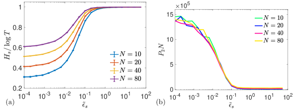
Figure 2: The RLM transition can be encountered by lowering the surface temperature $\epsilon_{s}$. Curves are shown at $T=1000$, $\tilde{\epsilon}_{d}\approx 0.03$, and indicated values of $N$; (a) the surface entropy drops around $\tilde{\epsilon}_{s}\approx 1/\log T$, while (b) the surface order parameter $P_{2}$ increases as $\tilde{\epsilon}_{s}$ is lowered.

Now, by a standard argument Parisi (1988) the Boltzmann entropy of configurations is equal to the Shannon entropy of the probability distribution over configurations. This latter quantity can be written as the entropy of forests at given $m$ and $\ell$, plus the conditional entropy of hidden configurations on those trees, plus the conditional entropy of leaves on those configurations. Each of these entropies can be written as the corresponding rate multiplied by the number of symbols. There are $\ell$ observable symbols and $2\ell-m$ hidden symbols, but all roots are set to the start symbol. Thus

$$S_{RS}=S_{\text{forest}}(\ell,m)+(2\ell-2m)H_{d}+\ell H_{s|d},$$ (8)

where $H_{s|d}$ is the conditional entropy rate of observable symbols, given the hidden ones. These configurational entropies are trivial at $\tilde{\epsilon}_{d},\tilde{\epsilon}_{s}=\infty$ so that we can write

$$(\ell-m)\log(gN^{2}/h)+\ell\log(gTh)+S_{\ell,m}$$

$$=S_{RS}(\tilde{\epsilon}_{d}=\infty,\tilde{\epsilon}_{s}=\infty)$$

$$=S_{\text{forest}}(\ell,m)+(2\ell-2m)\log N+\ell\log T$$

The factors of $\log N$ and $\log T$ cancel from this equality, as they must. As a result we obtain $S_{\text{forest}}(\ell,m)$ and finally

$$S_{RS} =S_{\text{forest}}(\ell,m)+(\ell-m)\log(N^{2})+\ell\log(T)$$

$$\qquad-\frac{\ell}{4\tilde{\epsilon}_{s}}-\frac{\ell-m}{4\tilde{\epsilon}_{d}}.$$ (9)

Comparing with (8) and noting that this equation must hold for all $\ell,m$ (with $\ell,m\to\infty,\ell/m$ finite ), we deduce

$$H_{d}=\log N-\frac{1}{8\tilde{\epsilon}_{d}},\qquad H_{s|d}=\log T-\frac{1}{4\tilde{\epsilon}_{s}},$$ (10)

in the replica-symmetric approximation. Since these entropies cannot be negative, they give lower bounds on the validity of the replica-symmetric approximation. At small enough $\tilde{\epsilon}_{d}$ or $\tilde{\epsilon}_{s}$, the approximations used to derive (10) must break down. It also follows from this that the normalized entropies $H_{d}/\log N$ and $H_{s|d}/\log T$ should collapse with $\tilde{\epsilon}_{d}\log N$ and $\tilde{\epsilon}_{s}\log T$, respectively.

Note that DeGiuli (2019) measured $H_{s}$, not $H_{s|d}$. In general the Bayes rule for conditional entropy is $H_{s|d}=H_{s}-H_{d}+H_{d|s}$. When $\tilde{\epsilon}_{s}$ is small, then knowing the observable symbols also fixes their POS tags, so $H_{d|s}\approx 0$ and $H_{s}(\tilde{\epsilon}_{s}\ll 1)\approx H_{s}-H_{d}$. However when $\tilde{\epsilon}_{s}$ is large, then knowing the hidden symbol tells you nothing about the observable symbol, so $H_{s|d}\approx H_{s}$. Thus generally we expect that as a function of $\tilde{\epsilon}_{s}$, $H_{s}$ behaves similarly to $H_{s|d}$.

These results indicate that the RLM transition can be probed by fixing $\tilde{\epsilon}_{d}$ and lowering $\tilde{\epsilon}_{s}$. Since this will be relevant for comparison with human data, we now show that this prediction is verified by numerics.

I.1 The RLM transition is encountered by increasing surface heterogeneity

We simulated the RLM with $T=1000$ and $\tilde{\epsilon}_{d}\approx 0.03$ at various values of $N$ and $\tilde{\epsilon}_{s}$. For each parameter value, 60 distinct grammars were constructed, and 200 sentences were sampled for each grammar. The results for the surface entropy are shown in Fig.2; as predicted by theory, the entropy begins to drop from its trivial value at $\tilde{\epsilon}_{s}\approx 1/\log T\approx 0.1$.

Since $\tilde{\epsilon}_{d}$ is fixed as $\tilde{\epsilon}_{s}$ varies, there is no variation in the hidden parts of the derivations: the quantities shown in DeGiuli (2019) to quantify the RLM transition, like the deep entropy $H_{d}$ and the order parameter $Q_{2}$, are flat as $\tilde{\epsilon}_{s}$ varies. Instead the transition can be quantified by the surface analog of the order parameter $Q_{2}$. For a surface rule $a\to B$ define

$$P_{aB}(M,O)=\langle\delta_{\sigma_{\alpha},a}(T\delta_{o_{\alpha},B}-1)\rangle,$$ (11)

averaged over all surface vertices $\alpha$ and over all derivations. Here $\sigma_{\alpha}$ is the hidden symbol and $o_{\alpha}$ the observable one. $P$ measures how the application of this rule differs from a uniform distrbution. An Edwards-Anderson type order parameter for surface structure is

$$P_{2}=\sum_{a,B}\overline{P_{aB}^{2}},$$ (12)

where $\overline{\;\;}$ is an average over grammars. This quantity is shown in Fig.2b. As expected, $P_{2}$ increases from a small value at high $\tilde{\epsilon}_{s}$ around the transition point.

II Learning a context-free grammar

Now we consider the learning problem. How does a child actually learn the specific grammar of its environment?

Our goal is not to completely answer this question, but simply to motivate why and how the symmetry of symbols should be explicitly broken. As a simple model, we suppose that the speaker utters sentences by drawing them from a stochastic grammar, which we take to be context-free. In a stochastic grammar, the weights quantify their frequency of use, which, for learners, is a proxy for their correctness. When all the weights are equal, nothing is known, and the grammar samples uniform noise (‘babbling’). In contrast, when the weights have a wide distribution, the grammar is highly restrictive and the output sentences are highly non-random.

The learning scenario suggested in DeGiuli (2019) was quite generic: suppose the child knows, possibly due to hardware constraints, that it is learning a CFG. Initially they know nothing of weights, so they start at $\epsilon_{d}=\epsilon_{s}=\infty$. Their initial speech will be uniform random noise. Now, as they try to mimic their caregivers, we assume that the child tunes the grammar weights. In doing so the corresponding values of $\epsilon_{s}$ and $\epsilon_{d}$, which could be defined from (4), will inevitably decrease. Then, the prediction of the RLM is that the entropy of the child’s output will remain high for some time, until quite suddenly it begins to decrease. At this point the child’s speech begins to convey information.

This scenario is quite schematic. Let us try to make it more concrete.

Consider first an optimal learning scenario. The child hears sentences $\gamma$, with words $o_{j}^{\gamma},j=1,\ldots,\ell_{\gamma}$, and wants to find the optimal grammar that produces them. It is natural to maximize the log-likelihood of the grammar, given the data, given by

$${\mathscr{L}}(M,O;o)=\log\mathbb{P}(o|M,O),$$ (13)

which is considered as a function of the grammar, with fixed sentences $\{o\}$. The sentence probability is

$$\mathbb{P}(o|M,O) =\prod_{\gamma}\sum_{\mathscr{T}_{\gamma},\sigma^{\gamma}_{k}}\mathbb{P}(o^{\gamma},\sigma^{\gamma},\mathscr{T}_{\gamma}|M,O)$$ (14)

$$=\prod_{\gamma}\frac{1}{Z}\underbrace{\sum_{\mathscr{T}_{\gamma},\sigma^{\gamma}_{k}}e^{-E(o^{\gamma},\sigma^{\gamma},\mathscr{T}_{\gamma};M,O)}}_{\equiv Z(o^{\gamma})},$$ (15)

where $Z(o^{\gamma})$ is then a partition function restricted to the given sentence $o^{\gamma}$. In principle, the child can estimate these quantities by speaking: every sentence they speak adds a contribution to the denominator $Z$. If they feel that their caregiver understood them, then they also add a contribution to the numerator $Z(o^{\gamma})$.

Unfortunately computing these restricted partition functions is difficult, both analytically, and for the child. So we consider a simpler, more idealized scenario. The child keeps track of a lexicon

$$\{tree,mama,toy,book,open,close,eat,sleep,up,down,\ldots\},$$

how many times they’ve heard each word, and also the categories to which each word belongs

$$\{noun,verb,adjective,\ldots\},$$

called part-of-speech (POS) tags.

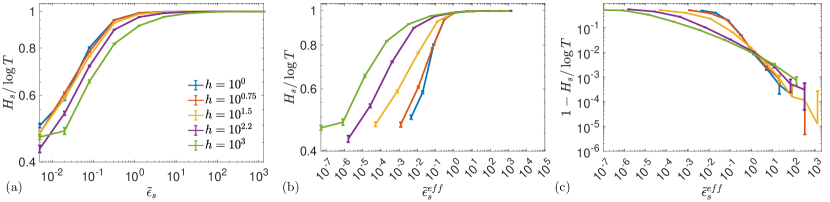
Figure 3: The RLM transition is robust to the addition of a Zipfian surface bias. Curves are shown at $T=100$, $\tilde{\epsilon}_{d}\approx 0.03$, and indicated values of bias strength $h$; (a) the surface entropy versus $\tilde{\epsilon}_{s}$; (b) the surface entropy versus an effective $\tilde{\epsilon}_{s}(\tilde{\epsilon}_{s},h)$ (see text). The onset of nontrivial surface entropy occurs at approximately $\tilde{\epsilon}_{s}^{eff}\approx 1$, but its development is weaker at larger biases.

The child thus obtains an estimate $\tilde{\rho}_{aB}$ of the joint word & POS frequency, $\rho_{aB}$. Then they maximize the likelihood of $\tilde{\rho}$,

$${\mathscr{L}}(M,O;\tilde{\rho}) =\log\mathbb{P}(\tilde{\rho}|M,O)$$ (16)

$$=\log\sum_{\{\mathscr{T},\sigma,o\}}\delta_{\rho(o,\sigma),\tilde{\rho}}\mathbb{P}(\mathscr{T},\sigma,o|M,O)$$ (17)

where $\rho(o,\sigma)_{aB}$ is the count of word $B$ and POS tag $a$ in the text of total length $\ell$, i.e.

$$\rho(o,\sigma)_{aB}=\sum_{j=1}^{\ell}\delta_{o_{j},B}\delta_{\sigma_{j},a}$$ (18)

The Kronecker $\delta$ in (17) counts only texts with the right number of each word and POS tag. We have

$$\delta_{\rho(o,\sigma),\ell\tilde{\rho}} =\prod_{a=1}^{N}\prod_{B=1}^{T}\delta_{\rho(o,\sigma)_{aB},\tilde{\rho}_{aB}}$$ (19)

$$=\prod_{a,B}\int_{0}^{2\pi}\frac{d\lambda_{aB}}{2\pi}e^{i\lambda_{a,B}(\rho(o,\sigma)_{aB}-\tilde{\rho}_{aB})}$$ (20)

$$\equiv\int{\mathscr{D}}\lambda\;e^{i\sum_{a,B}\lambda_{a,B}(\sum_{j=1}^{\ell}\delta_{o_{j},B}\delta_{\sigma_{j},a}-\tilde{\rho}_{aB})}$$ (21)

The energy depends on the words through the term

$$\sum_{a,B}\rho_{aB}\log O_{aB}=\sum_{a,B}\left[\sum_{j=1}^{\ell}\delta_{o_{j},B}\delta_{\sigma_{j},a}\right]\log O_{aB}$$ (22)

which has the same dependence on the text and POS tags. So we can write

$${\mathscr{L}}(M,O;\tilde{\rho})=\log\frac{1}{Z}\sum_{\{\mathscr{T},\sigma,o\}}\int{\mathscr{D}}\lambda\;e^{-i\lambda:\tilde{\rho}}e^{-E(\mathscr{T},\sigma,o|M,O(\lambda))}$$ (23)

where

$$\log O(\lambda)_{aB}=\log O_{aB}+i\lambda_{aB}$$ (24)

is a shifted surface grammar (in the complex plane). Note however that when a saddle point is attained (as will be the case for large texts), $i\lambda$ will be real, so that the grammar is real-valued as it must be.

Finally ${\mathscr{L}}$ becomes

$${\mathscr{L}}(M,O;\tilde{\rho})=\log\frac{1}{Z}\int{\mathscr{D}}\lambda\;e^{-i\lambda:\tilde{\rho}}Z(M,O(\lambda)),$$ (25)

so the likelihood depends on a shifted grammar. If we can evaluate this then we can derive the maximum-likelihood learning strategy, under the given assumptions.

However ${\mathscr{L}}$ is evaluated, the natural learning strategy on the grammars is simply to go in the gradient of increasing likelihood:

$$\frac{dM_{abc}}{dt} =k\frac{\partial{\mathscr{L}}}{\partial M_{abc}}$$ (26)

$$\frac{dO_{aB}}{dt} =k\frac{\partial{\mathscr{L}}}{\partial O_{aB}},$$ (27)

where $k$ is the learning rate.

Roughly speaking, ${\mathscr{L}}$ is a difference of (minus) free energies: that of the RLM in the presence of a biased grammar (to match the observed $\tilde{\rho}$), but subtracting off the original RLM free energy. Thus the simple picture of DeGiuli (2019) is slightly modified: the learning scenario can be viewed as a free energy descent, but only along the directions that lower the free energy coupled to the correct biased grammar; if a change in the grammar equally affects $Z(M,O(\lambda))$ and $Z(M,O)$, then it will cancel out of ${\mathscr{L}}$.

Let us try to understand (25) better. It involves the RLM partition function for a biased $O$ matrix. Note in general that

$$\frac{\partial\log Z}{\partial\log O_{aB}}=\frac{1}{Z}\sum_{\{\mathscr{T},\sigma,o\}}\rho_{aB}\;e^{-E}=\langle\rho_{aB}\rangle.$$ (28)

Now it is known that natural languages exhibit Zipf’s law: the probability of a word decreases as a power law of its rank. Thus $\rho_{aB}$ will exhibit such behavior, and by this computation, so should the dependence of $\log Z$ on $\log O_{aB}$. Thus to understand $Z(M,O(\lambda))$ we should simulate the RLM in the presence of a bias $i\lambda$, which we take to have a Zipfian form. We consider this next.

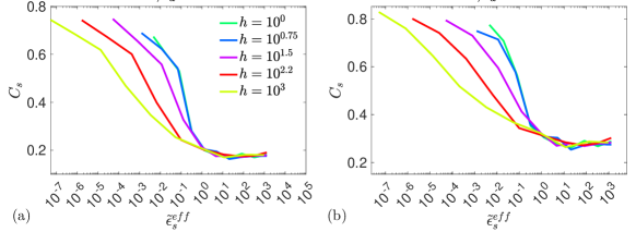
Figure 4: The clustering coefficient of word graphs increases at the RLM transition, for $T=100$ and indicated Zipfian biases, with strength $h$. Both (a) directed and (b) undirected graphs show a similar increase of clustering around the transition point $\tilde{\epsilon}_{s}^{eff}\approx 1$.

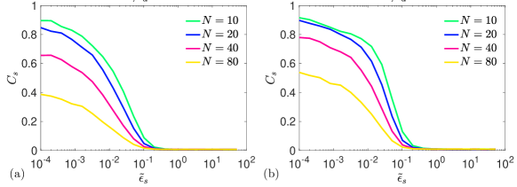
Figure 5: The clustering coefficient of word graphs increases at the RLM transition, for $T=1000$ and indicated $N$. Both (a) directed and (b) undirected graphs show a similar increase of clustering around $\tilde{\epsilon}_{s}\approx 0.1$.

III RLM with a bias

The learning scenario motivates considering the RLM with a bias in the surface grammar. Consider

$$\log O^{\prime}_{aB}=\log O_{aB}+h_{aB}$$ (29)

where $h$ is the bias, and $O$ is given the distribution from the RLM. Then $O^{\prime}$ has the distribution

$$\mathbb{P}(O^{\prime}) \propto\prod_{a,B}\frac{1}{O_{aB}}e^{-\tilde{\epsilon}_{s}\sum_{a,B}\log^{2}(O^{\prime}_{aB}e^{-h_{aB}}/\overline{O})}$$ (30)

$$\propto\prod_{a,B}\frac{1}{O^{\prime}_{aB}}e^{-\tilde{\epsilon}_{s}\sum_{a,B}\log^{2}(O^{\prime}_{aB}/\overline{O})}e^{\tilde{\epsilon}_{s}\sum_{a,B}h_{aB}\log O^{\prime}_{aB}/\overline{O}}$$ (31)

In order to disentangle the effect of the bias from that of $\epsilon_{s}$, we take $h_{aB}\propto 1/\tilde{\epsilon}_{s}$. As a Zipfian form, we consider

$$h_{aB}=\frac{h}{\tilde{\epsilon}_{s}}\frac{1}{B},$$ (32)

where we arbitrarily order the words in decreasing rank. The scalar $h$ is the bias strength.

We simulated the RLM with Zipfian bias and a variety of field strengths, for $T=100$ and $\tilde{\epsilon}_{d}\approx 0.03$. The resulting $H_{s}$ is shown in Fig.3. The RLM transition is present in all cases, but its position depends on the bias strength $h$. A larger bias causes the transition to occur earlier (at higher $\tilde{\epsilon}_{s}$). This is intuitively clear, as the RLM transition was shown to induce the breaking of symmetries among symbols DeGiuli (2019); since the bias breaks this symmetry explicitly, the transition occurs at higher $\tilde{\epsilon}_{s}$.

Inspecting Fig. 3a, it appears as though the data for different magnitudes of $h$ (‘bias strengths’) should collapse with some rescaled version of $\epsilon_{s}$. This suggests that a simple model may capture the dependence on the bias. The transition discussed in DeGiuli (2019); De Giuli (2019, 2022) is controlled by the heterogeneity of the grammar, measured in the original model by (3), which satisfy (4). Thus we can see how $\overline{s_{s}}$ is renormalized by the bias. We evaluate

$$\overline{s_{s}(h)} \equiv\frac{1}{NT}\sum_{a,B}\overline{\log^{2}\left[\frac{O_{aB}e^{h_{aB}}}{\overline{O}}\right]}$$ (33)

$$=\frac{1}{NT}\sum_{a,B}\int\frac{dO_{aB}}{O_{aB}\sqrt{\pi/\tilde{\epsilon}_{s}}}\log^{2}\left[\frac{O_{aB}e^{h_{aB}}}{\overline{O}}\right]e^{-\tilde{\epsilon}_{s}\log^{2}\left[\frac{O_{aB}}{\overline{O}}\right]}$$

$$=\frac{1}{NT}\sum_{a,B}\int\frac{do_{aB}}{\sqrt{\pi/\tilde{\epsilon}_{s}}}\big{(}o_{aB}+h_{aB}\big{)}^{2}e^{-\tilde{\epsilon}_{s}o_{aB}^{2}}$$

$$=\frac{1}{NT}\sum_{a,B}\left[\frac{1}{2\tilde{\epsilon}_{s}}+(h_{aB})^{2}\right]$$

$$=\frac{1}{2\tilde{\epsilon}_{s}}+\overline{h^{2}}$$ (34)

We can define a renormalized $\tilde{\epsilon}_{s}$ by

$$\frac{1}{2\tilde{\epsilon}_{s}^{eff}}=\frac{1}{2\tilde{\epsilon}_{s}}+\overline{h^{2}}$$ (35)

As shown in Figs. 3b, this approximately collapses the initial decay of $H_{s}$ from its trivial value. Looking at this initial decay on a logarithmic scale (Fig 3c), all curves appear to cross at a common point $\tilde{\epsilon}_{s}^{eff}\approx 1$.

We also simulated the RLM with a staggered field of the form $h_{aB}=h/\tilde{\epsilon}_{s}\times g_{B}$, where $g_{B}$ takes only three values $1,\sqrt{1/T},$and $1/T$, for the first, second, and third third of the symbols, respectively. The form and scaling is chosen to have a similar overall amplitude as the Zipfian bias. We found that for the same values of $h$ as above, there was no effect of the bias on $H_{s}$. We return to this later.

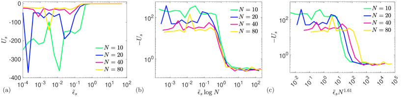
Figure 6: Binder cumulant of observable word distribution, for $T=1000$ and indicated $N$. (a) This quantity begins to differ from 0 around $\tilde{\epsilon}_{s}\approx 1$, as expected. (b,c) On a logarithmic axis, the onset appears to collapse with a logarithmic factor of $N$, but not the power-law suggested in Nakaishi and Hukushima (2022).

IV Comparison with human data

How does the RLM compare to first language acquisition in children?

In previous work, syntactic networks were built from data of children’s utterances between 22 and 32 months of age Corominas-Murtra et al. (2009), with data from the Peters corpora Bloom et al. (1974, 1975). The networks were built from dependency structures, with a mix of automated and manual procedures. These structures are graphs that connect observable symbols, related but distinct from phrase structure trees. A variety of network-theoretic quantities showed a clear transition around 24 months of age; for example, both the word degree (the number of other words used with a given word) and the clustering coefficient (measuring the extent to which words are clustered) increase dramatically at this transition.

If the RLM is to apply to first language acquisition, then we should be able to see similar behaviors in these quantities. However, the syntax trees are not equivalent to the dependency graphs. We build approximate dependency graphs as follows: we simply take the observed sentences $(o_{1},o_{2},\ldots,o_{j},\ldots)$ and add a link to the graph from $B$ to $A$ if $o(j)=B,o(j+1)=A$, for some observable symbols $A$ and $B$ and index $j$. This directed graph includes many true dependency relations, but also spurious ones that would be absent in a more complete analysis. It gives a first approximation to the dependency graphs. We investigated the clustering coefficient both for the directed graph, constructed as above, and the undirected graph constructed by adding the reverse links. The resulting clustering coefficients are shown in Fig. 4 and Fig 5. As the bias is varied, a clear increase is observed around $\tilde{\epsilon}_{s}^{eff}\approx 0.1$, consistent with the drop in sentence entropy. Similarly, as $N$ is varied the clustering also increases around the transition point.

The linguistic interpretation of this behavior is interesting Corominas-Murtra et al. (2009): the transition marks the point where the child begins to use functional items like $a$ or $the$ to connect many words. It thus represents the learning of a particular class of grammatical rules.

Finally, Corominas-Murtra et al. (2009) also looked at the degree distribution of dependency graphs, finding that below the transition graphs were scale-free with $\mathbb{P}(d_{s})\sim 1/d_{s}^{1.3}$. As discussed in the Appendix, this is consistent with what we find in our sentence graphs. Although a quantitative comparison is suspect because we do not create true dependency structures, this further supports that the RLM captures the initial onset of learning grammatical structure in first language acquisition.

V Finite-size scaling

True thermodynamic phase transitions only occur in the thermodynamic limit, because in a finite system, the partition function is an analytic function of control parameters. In the RLM, there are 2 distinct ways in which systems can be large: first, the sentence size $\ell$ gives the size of derivation structures, while $N$ and $T$ are the alphabet sizes, controlling the potential complexity of grammars. For this reason, in DeGiuli (2019) the senior author tuned the control parameters such that sentences were large (with a cutoff $\ell_{max}\sim 1000$), and moreover crucial observables were shown at various $N$. The existence of finite-size scaling in $N$ over an appreciable range from $N=10$ to $N=40$, and here up to $N=80$, shows that the basic phenomena of the RLM are not particular to small or large $N$.

A recent work Nakaishi and Hukushima (2022) questioned whether the RLM shows a true thermodynamic phase transition. By a combination of analytic and numerical arguments, the authors argue that there is no phase transition at finite $\tilde{\epsilon}_{d}$ and finite $N$ in the RLM. However, as already shown in DeGiuli (2019), to obtain satisfactory collapse of the data, quantities need to be collapsed with $\tilde{\epsilon}_{d}\log^{\alpha}N$, where $\alpha=1$ or $\alpha=2$ depending on the quantity considered. This is confirmed by theory that predicts $\alpha=1$, see for example (10) (after division by $\log N$ to compare with numerical results).

Nakaishi and Hukushima (2022) measured in particular the Binder cumulant

$$U=1-\frac{\langle(\pi_{a}-\langle\pi_{a}\rangle)^{4}\rangle}{3\langle(\pi_{a}-\langle\pi_{a}\rangle)^{2}\rangle^{2}},$$ (36)

which is 0 if $\pi_{a}$ is Gaussian, and nonzero otherwise. Here $\pi_{a}$ is the empirical probability of observing hidden symbol $a$, related to the order parameter $Q_{2}$. Nakaishi and Hukushima (2022) found that $U$ has a dip at the transition, which becomes infinitely deep as $N\to\infty$, suggesting that the RLM becomes a true thermodynamic phase transition in this limit. Nakaishi and Hukushima (2022) suggest that the $\tilde{\epsilon}_{d}$ at which the minimum of $U$ is obtained goes to zero as $1/N^{1.61}$ but their fit is suspect: at the largest values of $N$ that they use (only $N=10$) the plot of $\log\tilde{\epsilon}_{d}$ versus $\log U$ has a distinct curvature, indicating that functional dependence on $N$ is not a power-law. It would indeed be very strange if $U$ did not collapse with $\tilde{\epsilon}_{d}\log^{\alpha}N$ as all other quantities do. The difference between $N^{1.61}$ and $\log^{2}N$ in the range of small $N=1,\ldots,10$ considered by Nakaishi and Hukushima (2022) is slight.

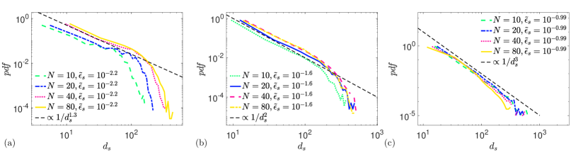
Figure 7: Degree distribution of sentence graphs at indicated values of $N$ and (a) $\tilde{\epsilon}_{s}=10^{-2.2}$, (b) $\tilde{\epsilon}_{s}=10^{-1.6}$, (c) $\tilde{\epsilon}_{s}=10^{-0.99}$. In all cases an approximate power-law regime can be discerned. The shown lines have exponents $1.3,2,$ and $3$, for (a,b,c), respectively.

We measured the same quantity over an ensemble controlled by $\tilde{\epsilon}_{d}$ but found that the fluctuations in this quantity were huge, indicating that it is not self-averaging. Instead we found cleaner measurements of the Binder cumulant of $\pi_{B}$, the distribution of observable symbols, in the ensemble considered above, dependent upon $\tilde{\epsilon}_{s}$. As shown in Fig.7, $U_{s}$ begins to differ from zero at the transition. On logarithmic axes, this onset appears to collapse with a logarithmic factor of $N$, but not the power law $N^{1.61}$ reported in Nakaishi and Hukushima (2022); the much larger range of $N$ considered here allows us to distinguish these collapses much easier than would be possible in the range $N=1,\ldots,10$. When the bias $h$ is varied, a similar behavior is observed (not shown).

It was mentioned by Nakaishi and Hukushima (2022) that the behavior of the Binder cumulant is similar to that observed in the 3D Heisenberg spin glass Imagawa and Kawamura (2002). Thus, contrary to the title of Nakaishi and Hukushima (2022), the results within actually support the existence of the RLM transition, in the limit $N\to\infty$, in appropriately rescaled variables. Since true thermodynamic phase transitions reside in universality classes, with a whole host of irrelevant variables, this further supports the robustness of the RLM as a simple model of syntax.

VI Discussion

In the Principles & Parameters scenario for first language learning Chomsky (1993), the task of learning syntax is reduced to the setting of a small number of discrete parameters, usually considered to be binary Shlonsky (2010). Ongoing debate surrounds the detailed taxonomy of parameters and associated categorization of language, but regardless of these details, the scenario suggests that learning will occur in a series of discrete steps. Observables that quantify learning should then also show discrete steps.

Instead, human data from Corominas-Murtra et al. (2009) as well as the RLM both suggest a single learning transition, with continuous (although in some cases abrupt) variation in observables. In the RLM this statement is robust to the inclusion of a bias, reflecting heterogeneity in the environment. One may wonder if the specific Zipfian bias considered above is itself too smooth to see a series of discrete transitions. To this end, we also tested a bias taking on only 3 values. Over the same range of bias strengths shown above, this bias did not have any effect on the sentence entropy. Thus, in all cases considered, the RLM transition is unimodal, matching that seen in human data.

Of course, it may be that discrete transitions can be only be detected by sufficiently sensitive order parameters. But if for simplicity we set aside this scenario, and take seriously the observations of a continuous learning process, then it raises questions for first language acquisition. A continuous learning process suggests that what is learned are weights (or probabilities) rather than discrete rules. Frequency effects are indeed ubiquitous in first language acquisition Ambridge et al. (2015), and there are proposals on how measured frequencies can be used to infer rules Yang et al. (2017). Moreover, the recent successes of machine learning in natural language processing Chang and Bergen (2023) are invariably using approaches with parameters that can be continuously tuned during the training process. Thus the notion of discrete syntactic parameters that are set during learning appears overly simplistic, and may fail to account for the diversity of human languages, as has been argued by linguists and psychologists, with vociferous debate Evans and Levinson (2009). Instead our results suggest that learning is continuous; after the RLM transition, the entropy of children’s speech continuously decreases, and concominantly, the grammar becomes more and more certain.

VII Conclusion

The Random Language Model was introduced in DeGiuli (2019) as a simple model of language. We showed here that the RLM transition can be encountered by a change in properties of observable sentences, is robust to the inclusion of a bias, and is apparently a sharp thermodynamic transition as $N\to\infty$, in appropriately rescaled variables. A comparison with human data Corominas-Murtra et al. (2009) supports that the RLM transition is equivalent to that experienced by most children in the age 22-26 months in the course of first language acquisition.

In future work, two avenues look promising: first, although limited by availability of quantitative data, more attempts to make a quantitative comparison with human data would be worthwhile; second, the astounding success of machine learning models to model natural language, and the lack of a theory to explain this, suggest that the RLM might shed light on this process. Indeed, the RLM captures several features of real-world data (long-range correlations, hierarchy, and combinatorial structure) that are missing from most physics models, and needed to understand modern deep neural networks Mézard (2023).

Finally, the search for an analytical solution to the RLM is ongoing. A promising approach De Giuli (2019, 2022) represents syntax trees as Feynman diagrams for an appropriate field theory, but this falls short of a complete solution. The results of Nakaishi and Hukushima (2022), as well as the results here, suggest that one should look for a solution in the idealized limit $N\to\infty$.

Acknowledgments: EDG is supported by NSERC Discovery Grant RGPIN-2020-04762.

VIII Appendix – Degree distributions of sentence graphs

To compare with the degree distributions measured in Corominas-Murtra et al. (2009), we measured the degree distribution of our sentence graphs. We find that a power-law regime can be discerned, but with an exponent that depends on $\tilde{\epsilon}_{s}$. At $\tilde{\epsilon}_{s}=10^{-2.2}$, the exponent matches what was observed in Corominas-Murtra et al. (2009), but we note that this result does not appear to be stable at lower $\tilde{\epsilon}_{s}$, where a hump develops at large degree.

References

- Post (1943) E. L. Post, American journal of mathematics 65, 197 (1943).
- Chomsky (2002) N. Chomsky, Syntactic structures (Walter de Gruyter, Berlin, 2002).
- Hopcroft et al. (2007) J. E. Hopcroft, R. Motwani, and J. D. Ullman, Introduction to automata theory, languages, and computation, 3rd ed. (Pearson, Boston, Ma, 2007).
- Searls (2002) D. B. Searls, Nature 420, 211 (2002).
- Knudsen and Hein (2003) B. Knudsen and J. Hein, Nucleic acids research 31, 3423 (2003).
- Escudero (1997) J. G. Escudero, in Symmetries in Science IX (Springer, Boston, 1997) pp. 139–152.
- DeGiuli (2019) E. DeGiuli, Phys. Rev. Lett. 122, 128301 (2019).
- Corominas-Murtra et al. (2009) B. Corominas-Murtra, S. Valverde, and R. Solé, Advances in Complex Systems 12, 371 (2009).
- De Giuli (2019) E. De Giuli, Journal of Physics A: Mathematical and Theoretical 52, 504001 (2019).
- De Giuli (2022) E. De Giuli, Journal of Physics A: Mathematical and Theoretical 55, 489501 (2022).
- Parisi (1988) G. Parisi, Statistical field theory (Addison-Wesley, 1988).